Journal of Computational Physics 183, 400–421 (2002)doi:10.1006/jcph.2002.7190

PROST: A Parabolic Reconstruction of SurfaceTension for the Volume-of-Fluid Method

Yuriko Renardy1 and Michael Renardy2

Department of Mathematics and ICAM, 460 McBryde Hall, Virginia Tech, Blacksburg, Virginia 24061-0123E-mail: renardy@math.vt.edu

Received August 28, 2001; revised August 13, 2002

DEDICATED TO KLAUS KIRCHGAESSNER ON THE OCCASION OF HIS SEVENTIETH BIRTHDAY

Volume-of-fluid (VOF) methods are popular for the direct numerical simulation oftime-dependent viscous incompressible flow of multiple liquids. As in any numericalmethod, however, it has its weaknesses, namely, for flows in which the capillaryforce is the dominant physical mechanism. The lack of convergence with spatialrefinement, or convergence to a solution that is slightly different from the exactsolution, has been documented in the literature. A well-known limiting case forthis is the existence of spurious currents for the simulation of a spherical drop withzero initial velocity. These currents are present in all previous versions of VOFalgorithms. In this paper, we develop an accurate representation of the body forcedue to surface tension, which effectively eliminates spurious currents. We call thisalgorithm PROST: parabolic reconstruction of surface tension. There are severalcomponents to this procedure, including the new body force algorithm, improvementsin the projection method for the Navier–Stokes solver, and a higher order interfaceadvection scheme. The curvature to the interface is calculated from an optimal fit for aquadratic approximation to the interface over groups of cells. c© 2002 Elsevier Science (USA)

Key Words: volume-of-fluid method; continuous surface force; multiphase flow.

1. INTRODUCTION

The volume-of-fluid method is based on solving the flow equations on a rectangular grid,regardless of the geometry of fluid interfaces. These interfaces are reconstructed from thevalues of a color (or VOF) function which represents the volume fraction of one of the fluids

1 Supported by NSF-CTS 0090381, NSF-INT 9815106, ACS-PRF, NSF-SCREMS, NCSA.2 Supported by NSF-DMS 9870220, NSF-INT 9815106.

400

0021-9991/02 $35.00c© 2002 Elsevier Science (USA)

All rights reserved.

VOF-PROST 401

in each grid cell:

C(x) ={

1, fluid 1,

0, fluid 2.(1)

In the continuous surface force (CSF) algorithm [1–3], surface tension forces are computedas a body force,

f = ��n�S, (2)

where � is the coefficient of surface tension, � is the mean curvature, n is the normalto the surface, and �S is a delta function concentrated on the interface. Alternatively, thecontinuous surface stress (CSS) method [4, 5] represents surface tension as the divergenceof a stress tensor,

f = ∇ · T, T = [(1 − n ⊗ n)��S]. (3)

In the continuum limit,

n�S = −∇C, (4)

where C is the color function. On discretization, the derivatives of the color function arereplaced by finite differences. The problem is that finite difference approximations forderivatives of a discontinuous function are highly inaccurate. This leads to serious errorsin the computation of both the normal and the curvature. These errors are particularlyhighlighted in the classical example given in Section 4. The initial condition is a sphericaldrop with zero velocity (and at zero gravity), so that this exact solution should be preservedfor all time. However, previous VOF methods lead to the creation of spurious currents localto the interface. Although these spurious currents are small as long as the Ohnesorge number

Oh = (Ca/Re)1/2 (5)

(where Ca = �U/�, Re = Ua�/�, � is viscosity, U is speed, � is interfacial tension, ais length scale, and � is density) is sufficiently large, they do not disappear with meshrefinement, leading to nonconvergence of the method. The problem can be ameliorated bysmoothing the color function before taking derivatives [6]. To actually restore convergenceto the scheme, however, smoothing would have to be over a distance which is large relativeto the mesh size; this is unrealistic in practice. Moreover, smoothing leads to artifacts of itsown by effectively suppressing surface tension in high-curvature regions [7, 8].

The interface is reconstructed from the volume fraction function, usually as a linear inter-face per cell with the piecewise linear interface construction (PLIC) method. A potentiallymore accurate method is given in [9] for the two-dimensional case. The authors note thatwhat they really need is an equation for the interface given the color function, but thatthe reverse is easier. Given an exact formula for the interface, namely arcs of circles, theycalculate what the color function needs to be; they generate many such cases, which arestored in a data bank. They generate an empirical formula, which they fit to this data base.They postulate a third-degree polynomial to fit the data. The arcs of circles provide a higherdegree correction to the traditional linear interface of the PLIC method. They show that this

402 RENARDY AND RENARDY

drastically reduces the spurious currents. They remark that the method is extendable to threedimensions if a uniform grid with cubic cells is used. They suggest the use of sphericalsurfaces in place of circles. We remark, however, that this would not work because twoindependent principal radii of curvature are needed in 3D.

We also refer readers to the literature for other approaches to reduce spurious currentsby appropriate methods of interface reconstruction. In [10] a cubic spline is fitted to thevalues of the color function. The code of [11] also uses cubic splines but tracks the interfaceusing marker particles; the color function is reconstructed from the interface rather than theother way around. Both these schemes are limited to the two-dimensional case at this point.In [12] an algorithm is developed to reconstruct surface tension forces from a set of givenpoints on an interface in three dimensions without any a priori assumptions on connectivityof the interface. In contrast to our approach, the works of [11, 12] track rather than capturethe interface, i.e., the primary information is a set of points on the interface rather thanvolume fractions in grid cells.

In this paper, we introduce and test a novel algorithm for the computation of surfaceforces for the general three-dimensional case. Our algorithm is based on the VOF method,which reconstructs the interface from a color function. However, we refer to our methodas a sharp interface because the advection of the color function is based on a Lagrangianscheme which allows no diffusion (i.e., the color function changes form zero to one within amesh width). Unlike previous algorithms such as CSF or CSS, we never need to consider asmoothed color function. Instead, we calculate a least-squares fit of a quadratic surface to thecolor function for each interface cell and its neighbors. In 3D, there are 27 cells involved.The difference with the work of [9] is that we do not deal with empirical formulas anddata bases. Our surface tension algorithm leads to a second-order accuracy in the interfacereconstruction but is incompatible with the Lagrangian advection scheme described in [13]for PLIC, which is of low order. Therefore, it is necessary to advect the interface moreaccurately. In Section 3, a new higher order interface advection scheme is formulated. Oursurface tension algorithm together with our improved advection scheme comprise PROSTand result in the more accurate tracking of interfacial deformation.

In Section 4, we demonstrate that PROST can be used to effectively eliminate spuriouscurrents. Here, the code is begun with an exact solution, that of a spherical drop with zerovelocity, satisfying the governing equations, together with the body force of Eqs. (2) and(4):

f = −��∇C. (6)

If � is a constant (i.e., for a sphere), the surface tension force is cancelled by a pressuregradient and drives no flow. The key idea is that this still remains the case at the discretelevel, as long as ∇C and ∇ p are discretized by the same finite difference method (both∇C and ∇ p are singular at the interface, but they cancel each other out). Hence the crucialingredient in avoiding spurious currents is an accurate approximation to the curvature. Thispart of our algorithm is tested in Section 4. We show a comparison of the performance ofthe past CSF with smoothing, and the CSS without smoothing. The magnitudes of the spu-rious currents for the CSF and CSS schemes are shown in various norms, for spatial meshrefinements, and are shown to be nonconvergent or convergent only in certain norms. In com-parison, our method is shown to converge with spatial refinement and to produce no spuriouscurrents.

VOF-PROST 403

The entire PROST algorithm including the higher order advection scheme is appliedto three-dimensional drop deformation under simple shear in Section 5. Simulations for aspherical drop suspended in a second immiscible liquid, sheared between parallel plates,are compared with that of a boundary integral code with an adaptive mesh [14, 15]. Thisboundary integral code is expected to produce quite accurate results for the Stokes flowregime. The evolution to steady state is documented for CSF, CSS, and PROST. We showthat for both CSF and CSS, the drop shapes converge with spatial refinement to steady-statelengths that are slightly too long. The PROST simulation shows convergence with spatialrefinement toward the boundary integral results.

2. SHARP INTERFACE ALGORITHM FOR INTERFACIAL TENSION

We use the VOF code SURFER, which is described in [4, 16, 17]. There are three maincomponents to the code: (i) the interface tracking component based on the piecewise linearinterface construction method (PLIC) and a Lagrangian advection scheme, (ii) the Navier–Stokes solver based on a projection method and a multigrid solver for the pressure field,and (iii) the interfacial tension algorithm, CSF or CSS. Our basic scheme is that employedin SURFER++, which has additional algorithms and physics and has been continuallydeveloped [7, 18–26]. In this paper, we shall focus on the new aspects.

2.1. Approximation for Interface Shape

We need to identify those cells which contain the interface in order to determine theinterface normal and curvature. The color function is zero in one of the two fluids and onein the other, and in the code we call a cell, an interface cell, if the value of the color function,is between 10−8 and 1 − 10−8.

Figure 1 shows a sample grid, two-dimensional for simplicity. For each interface cell,such as the one at the arrow with center coordinate x0, we attach the neighbors and examinethe nine cells. In Fig. 1, four out of the nine cells contain the interface. For the central cell,

FIG. 1. Sample two-dimensional grid. The arrow points to an interface cell with center coordinate x0, andvolume fraction C . The interface is fitted with a quadratic surface through this cell plus its neighbors, a total ofnine cells in 2D. Here, four out of the nine are interface cells.

404 RENARDY AND RENARDY

the interface is fitted with a quadratic equation of the form

k + n · (x − x0) + (x − x0) · A(x − x0) = 0. (7)

In three dimensions, there are 27 cells around the center node x0 · n is a unit vector approx-imating the normal, and A is a symmetric matrix with the property that An = 0; that is, theaxis of the paraboloid is along n. This quadratic equation involves six parameters: one fork, two for n with normalization, and three for A. For any given choice of these parameters,we can compute the volume fraction v which the quadratic surface cuts out of a grid cell(details of this computation are described in Section 2.5). The parameters for the quadraticsurface can be organized as a six-dimensional vector q, which is to be determined in sucha way that

f (q) =∑

w(v − C)2 (8)

is minimized. Here the sum is over the given interface cell and all its neighbors, v is thevolume fraction in each cell determined by the quadratic surface, C is the value of thecolor function in the cell, and w is a weight discussed below. For reasons of computationalefficiency, we have modified this and extended the sum only over interface cells. For the 2Dcase in Fig. 1, q is a three-dimensional vector and v is the area under the parabola dividedby the total area of the cell. f (q) = ∑4

i=1(vi − Ci )2 must be minimized. Ideally, we wouldlike vi = Ci but this is four equations and there are three parameters for the parabola.

The reader may wonder why we restrict the quadratic terms by the constraint An = 0.The rationale for this is that other quadratic terms in (7) would be effectively of cubic order.As a simple illustration, consider a curve

y = ax2 + bxy + cy2; (9)

i.e., the curve passes through the origin and the normal is in the y-direction. We can rewritethe equation of the curve in the form

y = ax2 + abx3 + (ab2 + ca2)x4 + O(x5), (10)

i.e., only a really contributes at quadratic order, while b and c contribute at cubic and quarticorder.

Finally, we need to explain the weights included in (8). The simplest choice would beto simply set w = 1 in each cell. We modified this for two reasons. First, if an interfacepasses close to a corner of a cell, then the value of the color function is quite insensitiveto the position of the interface. If the interface intersects a corner at a generic angle and ismoved by a distance �, the color function only changes by O(�3). To deal with this issue,we introduce a weight factor

w1 = 1

C(1 − C) + �, (11)

which forces a better fit in cells where C is close to 0 or 1. Numerical experiments withdifferent values of � led us to the choice � = 0.01. Actually, this made no real differenceto the results of the simulation, but it reduced the number of cases where the optimizationalgorithm was slow to converge. A second, much more serious issue relates to the formation

VOF-PROST 405

of checkerboards. Consider an interface that is a graph z = f (x, y), where f is a stepfunction assuming constant values in a checkerboard pattern. No quadratic surface can fitsuch a checkerboard, and an unweighted sum in (8) does not produce a surface tension forceto suppress it. We saw such checkerboards emerge over time in some of our simulations.There is no numerical instability, but checkerboards represent a neutral mode which cangradually grow. As a mechanism for suppressing checkerboards, we introduce a weight w2,which equals 1 for the “central” cell, 1/2 for each cell sharing a face with it, 1/4 for eachcell sharing an edge with it, and 1/8 for each cell sharing a corner with it. Finally, w isequal to the product w1w2.

2.2. Optimal Fit

The basic algorithm for the least-squares optimization is that described in Sections A5.5.1and A5.5.2 of [27]. This algorithm is implemented in the IMSL package, but we chose towrite our own code rather than use IMSL because (as of the time we wrote our code) thispart of the IMSL package is not thread safe for open MP parallelism. To minimize thefunction f (q), we basically use the Newton iteration for finding zeros of ∇ f ; i.e.,

qi+1 = qi − (∇2 f (qi ))−1∇ f (qi ), i = 0, 1, 2, . . . , (12)

where q0 is the starting value. The derivatives of f are calculated by finite differenceapproximations. The Newton iteration is set up in the following way, to make sure thatf (qi+1) is less than for the previous iterate f (qi ). If the minimum is sufficiently close,then ∇2 f is positive definite. On the other hand, the finite difference approximation of thematrix ∇2 f may not be positive definite because of numerical errors. In order to hit a betteriterate, a constant is added to the diagonal to make it positive definite [27]. We note that theNewton iteration assumes f to be smooth, and our function is actually not smooth whenthe interface crosses a corner of a grid cell. To handle these cases, we modify the algorithmwhen f (qn+1) does not come out less than f (qn), |∇ f | is larger than a specified tolerance,or convergence is not obtained in a satisfactory number of steps. If this happens, we set

qn+1 = qn − �∇ f (qn), (13)

where � is chosen such that f (qn+1) is as small as possible. If this algorithm still does notachieve convergence, we do an alternating search along coordinate directions, each timesearching for the minimum along a line.

By combining these algorithms, we are able to obtain convergence of the optimizationalgorithm in almost all cases. Some exceptions occur as breakup is reached, and in thesecases we simply “give up” and stop the optimization algorithm after 200 steps.

To improve the mass conservation of the scheme, we adjust the value of k at the endof the optimization so that the value of the color function C in the central cell is fittedexactly (without such a correction, we do not obtain acceptable results for mass conserva-tion). We make an exception to this, however, if cells are almost empty or full, because, inthese cases, as mentioned above, a fairly large shift of the interface may be needed toachieve the right value of the color function. This shift would then produce a quite inac-curate interface, leading to interface reconstructions in certain cells which fit poorly withneighboring cells. A satisfactory compromise was achieved by adjusting k only for cellswith 0.02 ≤ C ≤ 0.98.

406 RENARDY AND RENARDY

The iteration for the optimization needs a starting value. At the initial time, we generatethis starting value from the analytic form of the initial interface. At subsequent times, thestarting value is the equation of the interface at the previous time step, updated by advection,as described below.

2.3. The Mean Curvature �

The surface tension force is now calculated as −��∇C , where � is calculated as 2tr(A),with A being the matrix from (7). This defines � at cell centers, while the components of ∇Care defined at the centers of the faces of a cell. We interpolate the value of � as a weightedaverage; that is, in the x-component, the combination �∂C/∂x is

[�

∂C

∂x

](xi−1/2, y j , zk

) = w1�(xi−1, y j , zk) + w2�(xi , y j , zk)

w1 + w2

×(

C(xi , y j , zk) − C(xi−1, y j , zk)

�x

), (14)

where

w1 = C(xi−1, y j , zk)(1 − C(xi−1, y j , zk)), w2 = C(xi , y j , zk)(1 − C(xi , y j , zk)). (15)

The rationale behind this weighting is that we expect the approximation to the curvature tobe more accurate when C is not close to 0 or 1. For example, if the cell at (xi−1, y j , zk) isnot an interface cell, then �(xi−1, y j , zk) is not defined there, but its weight w1 is zero, sothat the combination is zero.

2.4. Singular Part of Pressure Gradient

In our Navier–Stokes solver, we decouple the velocity and pressure fields with a projectionmethod [28]. At each time step, we first integrate the velocities as though the pressure termwere absent and then solve for the pressure to make the velocity divergence free. Namely,given the quantities at time level n, an intermediate velocity u∗ is calculated; i.e.,

u∗ − un

�t= −un · ∇un + 1

�(∇ · (�S) + F)n, (16)

where F includes gravity and the interfacial tension force, and S is the strain rate tensor. u∗

is not, in general, divergence free, and

un+1 − u∗

�t= −∇ p

�, (17)

where un+1 at time level n + 1 satisfies

∇ · un+1 = 0. (18)

When Eq. (17) is substituted into Eq. (18), a Poisson equation for the pressure field results:

∇ ·(∇ p

�

)= −∇ · u∗

�t. (19)

VOF-PROST 407

We can combine the equations above and obtain

un+1 − un

�t= −un · ∇un + 1

�(∇ · (�S) + F)n − ∇ p

�. (20)

In our code, however, we do not use the explicit scheme. For the velocity solution, weuse the semi-implicit method of [21], which is lengthy to write out in full. Here, therefore,we write it in symbolic form:

�u∗ − un

�t= Au∗ + B(un) + f,

(21)

�un+1 − u∗

�t= −∇ pn+1.

A represents the operator that acts on the term u∗ and B represents the one acting on un

and are given in [21]. Again, f is the body force which includes the singular surface tensionforce. Combining the two equations yields

�un+1 − un

�t= Aun+1 + B(un) + f − ∇ pn+1 + (�t)A(�∇ pn+1). (22)

The last term may be significant unless �t is very small, since p includes the singularpressure which is needed to balance surface tension. For this reason, we modify our schemeas follows:

�u∗ − un

�t= Au∗ + B(un) + f − ∇ p1,

(23)

�un+1 − u∗

�t= −∇ p2.

Here, p1 is chosen such that f − ∇ p1 is divergence free. Combining the two equations nowyields

�un+1 − un

�t= Aun+1 + B(un) + f − ∇(p1 + p2) + (�t)A(�∇ p2), (24)

which shows that since ∇ p2 is orders of magnitude smaller than ∇ p1, the O(�t) error termis much smaller. This algorithm measurably improves the size of the time step that can beused. For example, the results of Section 5 are obtained with 10 times the time-step sizeused in [8, 21, 22, 26, 29] and are more accurate.

2.5. Second-Order Algorithm for Volume Fraction

To complete the description of the numerical algorithm, we need to describe how wecalculate the volume which the quadratic surface given by (7) cuts out of a cell. That is, wewant to find the volume within the parallelepiped

x0 − �x/2 ≤ x ≤ x0 + �x/2,

y0 − �y/2 ≤ y ≤ y0 + �y/2, (25)

z0 − �z/2 ≤ z ≤ z0 + �z/2,

408 RENARDY AND RENARDY

where

k + n · (x − x0) + (x − x0) · A(x − x0) ≤ 0. (26)

A naive approach to computing the volume fraction would be to use a “pixel method,”i.e., to take a regularly spaced grid of points in a cell and determine the volume fractionby counting the number of points on the right side of the interface. This, however, ishopelessly slow and totally impractical. An exact analytical evaluation of the volume fractionis possible, and indeed we programmed it. We found, however, that this was about five timesslower than the algorithm we describe below and, even more serious, we were unable tocontrol round-off errors. For this reason, we settled for an approximate evaluation of thevolume fraction.

We can simplify the calculation if we assume that the mesh size is small and the curvatureis of order 1. First, we reorient our coordinates such that the largest component of n is inthe z direction and is positive. This will guarantee that within our mesh cell the interface isa graph z = g(x, y). Next, we can approximate g by a quadratic function, as follows. First,use the linear approximation in Eq. (7),

z − z0 ∼ − 1

n3(k + n1(x − x0) + n2(y − y0)), (27)

and second, we substitute this expression for z in the quadratic terms. We thus need to findthe volume under the graph of the function z = g(x, y) which lies above z = z0 − �z/2minus the volume which lies above z = z0 + �z/2. To find the volume which lies above,say z = z0 − �z/2, we find the intersection of the graph with the plane z = z0 − �z/2. Thisis a quadratic curve, and we need to integrate over the area which lies on one side of thecurve.

If the projection of the normal onto the x, y-plane is small, we can expect the quadraticcurve to have a high curvature, and in this case we use a seminumerical procedure, wherethe integration in one direction is carried out numerically. Otherwise, we use an analyticapproximation. We first, if necessary, cut the base rectangle into quadrants such that in eachquadrant the curve representing the interface is represented by a monotone function y(x).Next, the line of intersection is approximated by a straight line obtained from interpolatingbetween the intersection points with the edges of the rectangle. In this fashion, the problemis reduced to integrating a quadratic function over a set which is the union of rectanglesand triangles. This procedure determines the volume fraction in the cell (the volume of theintersection O(h5) divided by the cell volume O(h3)) to within an error of order h2, where

h = max(�x, �y, �z) (28)

is the spatial grid size.

3. HIGHER ORDER INTERFACE ADVECTION SCHEME

The original advection scheme in SURFER is based in a piecewise linear interface re-construction and a Lagrangian scheme which advects successively in the three coordinatedirections, To advect in the x-direction, for instance, let us consider the cell indexed by(i, j, k). The volume fraction in this cell is c(i, j, k). At each time step, fluid contained in

VOF-PROST 409

cell (i, j, k) can move to cells (i − 1, j, k), (i, j, k), and (i + 1, j, k). The three fractions aredetermined as follows. First, the right and left face of the cell are moved, respectively, withthe velocity lying at the nodal point at the center of each face, and the interface is subjectedto the affine deformation imposed by this motion. After deforming in this way, one deter-mines the amount of fluid which has moved to each neighboring cell by this deformation.

In the new scheme, we apply this same algorithm, with the difference that we use ourquadratic representation of the interface instead of a linear reconstruction. At each advectionstep, we update the equation of the interface as well as the values of the color function. Ifthe interface moves into new cells, we extrapolate the interface equation from a neighboringcell to define an interface equation in the new cell.

To improve the accuracy of the advection, we apply a “shear correction,” which takesaccount of the fact that the speed with which fluid 1 is advected in a cell may differ from theaverage speed because of shear. Since the difference in speed is small, of order h, we use aEulerian scheme based on fluxes. For each face of the cell, we then calculate the area on thisface which lies within fluid 1 and the center of mass of this area. We use linear interpolationfrom nodal values to determine a normal velocity at the center of mass. We then take thedifference between this velocity at the center of mass and the nodal velocity at the centerof the face of the cell. For this difference velocity, a volume flux is calculated from area ×normal velocity × time step. For each face of the cell, we determine the volume of fluidleaving the cell if this flux is outward. The volume remaining in the cell is the originalvolume minus the total volume leaving. Finally, the new value of the color function in eachcell is found by adding the volume remaining in that cell and the volume entering fromneighboring cells. We note that the linear interpolation of velocity near the interface is notcorrect unless the viscosity ration is 1, and hence the improvement of the shear correctionis only qualitative. A “better” alternative would then depend on the interpretation of whatexactly the nodal values of velocity represent. We do not attempt to address such issuessince, in any case, the proper treatment of discontinuities in the velocity gradient has notbeen addressed in other parts of the code, such as the momentum equation.

To calculate the area and center of mass, we can usually assume that the curve representingthe intersection of the interface and the face of the cell is close to a straight line. If this isthe case, we use an analytical approximation where the area is determined as a union ofrectangles and triangles which are found from the intersections of the interface with theedges. At points where the curvature is large, we use a numerical evaluation instead. For asmooth interface, this situation occurs when, for instance, the face of the cell is parallel tothe x, y-plane and the normal of the interface is close to the z-direction.

4. NUMERICAL RESULTS ON SPURIOUS CURRENTS

Spurious or parasite currents are described in [5] as vortices “in the neighborhood ofinterfaces despite the absence of any external forcing. They are observed with many surfacetension simulation methods, including the CSF method, the CSS method, and the lattice-Boltzmann method, in which they were first discovered.”

In this section, we compare the CSF, CSS, and PROST methods. The specific version ofthe CSF method we use is based on [1]; for the smoothing kernel we use the kernel K8 of [6].One smoothing iteration is used for the normal and two for the curvature. (Some alternativeimplementations of the CSF method, which lead to some improvement of spurious currents,are discussed in [6].)

410 RENARDY AND RENARDY

TABLE I

Norms of Velocity at 200th Time Step, ∆t = 10−5

�x L∞ L2 L1 Method

1/96 0.00179982 0.00008403 0.00001473 CSF1/128 0.00184090 0.00008542 0.000015391/160 0.00189053 0.00008596 0.000015691/192 0.00196880 0.00008627 0.00001569

1/96 0.00377043 0.00014183 0.00001920 CSS1/128 0.00358876 0.00012446 0.000016151/160 0.00360416 0.00011230 0.000014381/192 0.00398403 0.00010453 0.00001346

1/96 0.00002243 0.00000087 0.00000014 PROST1/128 0.00001309 0.00000053 0.000000091/160 0.00000954 0.00000041 0.000000071/192 0.00000568 0.00000023 0.00000004

Our computational domain is 1 × 1 × 1, the spatial mesh keeps �x = �y = �z, and thetime step is �t = 10−5. The boundary conditions are zero velocity at the top and bottomwalls, and periodicity in x- and y-directions. Initially, a spherical drop is centered at (0.5,0.5, 0.5), with radius a = 0.125 and surface tension � = 0.357. Both fluids have equaldensity, 4, and viscosity, 1. The initial velocity field is zero. The exact solution is zerovelocity for all time. In dimensionless terms, the relevant parameter is the Ohnesorge numberOh = (�2/��a)1/2 ∼ 2.37.

The amplitude Max |u | of the spurious currents is difficult to estimate a priori butRefs. [4, 5] find from direct measurements that they are of order 0.01�/�, leading to aReynolds number based on spurious currents, which is of the order 0.01/Oh2. At smallOhnesorge numbers, this can lead to troublesome flow instabilities. Table I verifies thisscaling for the CSF and CSS methods. The table shows the L∞, L2, and L1 norms of thevelocity field for the spurious currents. While the L∞ norm gives the maximum speed, theL2 and L1 norms indicate a measure in an average sense for the computational domain.Table II shows results for PROST with larger time steps, showing that entries of Table I areconverged with respect to time step. The scaling of spurious currents with �/� is obvious,since the surface tension force driving them is proportional to � and is counteracted byviscous damping. Since the PROST algorithm reduces spurious currents by two to threeorders of magnitude, it will also eliminate the instabilities at low Ohnesorge numbers.

TABLE II

Norms of Velocity at 20th Time Step, ∆t = 10−4

�x L∞ L2 L1 Method

1/96 0.00002156 0.00000084 0.00000014 PROST1/128 0.00001264 0.00000051 0.000000081/160 0.00000905 0.00000039 0.000000061/192 0.00000545 0.00000022 0.00000004

Note. This shows that the results in Table I for the PROST methodare converged with respect to the time step.

VOF-PROST 411

FIG. 2. CSF, velocity vector plot across centerline in the x–z-plane at 200th time step, �t = 10−5. These showthe locations of the spurious currents with mesh refinement, �x = 1/96, 1/128, 1/160. The relative magnitudesof the vectors are given in Table II.

These tables show the following:

1. For the CSF method, mesh refinement does not decrease the spurious currents in anyof the norms. In fact, they increase slightly in L∞ and L2 and stay about the same in L1. Toillustrate this, Fig. 2 shows the two-dimensional cross section of the drop in the x–z-plane.The spurious vortices are present at the same positions and spread over the same amount ofthe domain for all the meshes.

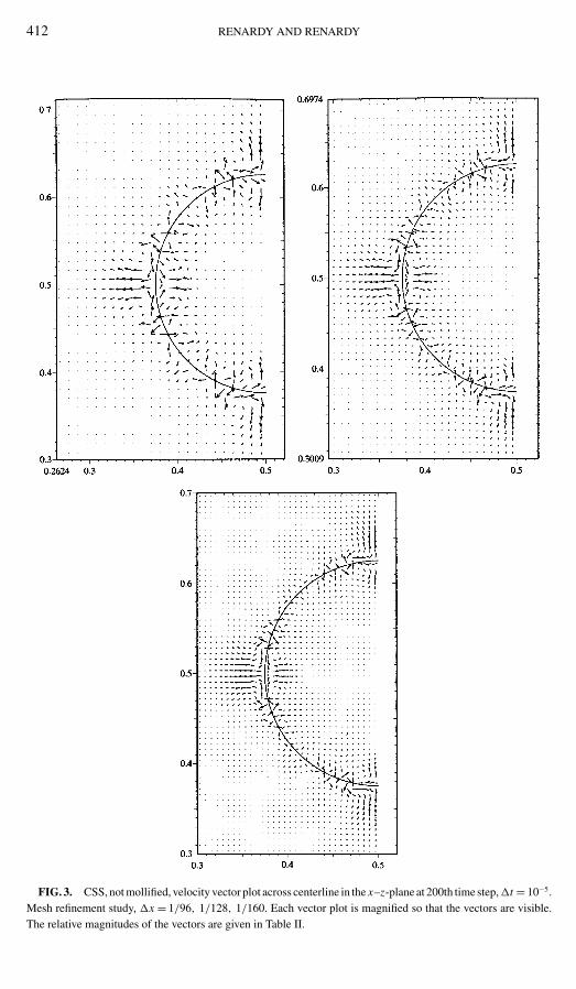
2. For theCSS method, mesh refinement does not decrease the L∞ norm of spuriouscurrents but decreases the L2 and L1. Figure 3 shows half of the cross section of the dropin the x–z-plane. With mesh refinement, the number of vortices increases, and they coverless domain.

3. For the PROST method, spurious currents are so small that they are effectively notpresent. This is no surprise. As we pointed out earlier, there would be NO spurious currentsif curvature were constant and our initial interface a sphere. The only reason the curvatureis not exactly constant is because the least-squares fit approximates the sphere as piecewiseparaboloids. The magnitude for the �x = 1/96 mesh is 1/100th that of CSF or CSS andthereafter decreases with mesh refinement with O(h), h = Max{�x, �y, �z}. Figure 4 plots

412 RENARDY AND RENARDY

FIG. 3. CSS, not mollified, velocity vector plot across centerline in the x–z-plane at 200th time step,�t = 10−5.Mesh refinement study, �x = 1/96, 1/128, 1/160. Each vector plot is magnified so that the vectors are visible.The relative magnitudes of the vectors are given in Table II.

VOF-PROST 413

FIG. 4. VOF-PROST, velocity vector plot across centerline in the x–z-plane at 200th time step, �t = 10−5.Variation of spurious current with mesh refinement, �x = 1/96, 1/128, 1/160. Each vector plot is magnified sothat the vectors are visible, the latter two plots being magnified much more than the first. The relative magnitudesof the vectors are given in Table II.

414 RENARDY AND RENARDY

FIG. 5. CFL numbers vs time steps (200), �t = 10−5. The CFL numbers remain the same order of magnitudeas that at the 200th time step.

the velocity vectors in comparison to Figs. 2 and 3. The three plots in Fig. 4 should not becompared for relative magnitudes. In order for the spurious currents to be discernible, the1/128 and 1/160 cases are magnified much more than for the 1/96 mesh. To obtain the truerelative magnitudes among the three meshes, we refer the reader to Table II. Figures 2–4and Tables I and II show that the locations of the spurious currents for PROST are similarto those of CSF, and that the magnitudes decay with spatial refinement.

Figure 5 shows the evolution of the Courant–Friedrichs–Levy number (CFL),

CFL = Umax�t/�x, Umax = max|u|. (29)

This is a measure of the L∞ norm of the spurious current. The figure shows the evolution ofthe CFL number over a longer time interval to show that it settles to some saturation level,and the sampling at the 200th time step for Table I is already at that magnitude.

5. NUMERICAL RESULTS ON DROP DEFORMATION

VOF-PROST is compared with the boundary integral method of [14, 30] for drop defor-mation under simple shear. The geometry is a Couette device, with a drop suspended in asecond liquid, and sheared by the motion of outer walls. A capillary number is defined by

Ca = a

�, (30)

where is the shear rate (normalized to 1 in the computations), is the viscosity of the matrixfluid, � is the interfacial tension coefficient, and a is the initial drop radius. At Ca = 0.35,

VOF-PROST 415

TABLE III

Table of Capillary Time, Physical Time, the Boundary Integral

Results, Results for Re = 0.0625 from VOF-CSF with (1) h = 1/128,

∆t = 5 × 10−4, (2) h = 1/128,∆t = 2 × 10−4

Capillary time Time B. I. Stokes CSF 1 CSF 2

0.000 0.000 0.997 0.999 0.9991.000 0.350 1.150 1.154 1.1542.000 0.700 1.265 1.277 1.2763.000 1.050 1.351 1.371 1.3674.000 1.400 1.422 1.447 1.4415.000 1.750 1.475 1.511 1.4956.000 2.100 1.521 1.554 1.5437.000 2.450 1.558 1.597 1.5828.000 2.800 1.586 1.629 1.6159.000 3.150 1.611 1.659 1.644

10.000 3.500 1.631 1.682 1.66515.000 5.250 1.691 1.757 1.73620.000 7.000 1.711 1.787 1.76130.000 10.500 1.718 1.815 1.77540.000 14.000 1.717 1.816 1.77650.000 17.500 1.717 1.816 1.776

the drop does not break up in Stokes flow. For our similations, we use a Reynolds numberof 0.0625, which should be small enough for the results to be only slightly different fromStokes flow.

Tables III and IV show the comparison of the boundary integral method with VOF-PROSTand VOF-CSF at Ca = 0.35 (the boundary integral method is validated against experiments

TABLE IV

Table of Capillary Time, Results for Re = 0.0625 from VOF-PROST

with (1) h = 1/96,∆t =10−3, (2) h = 1/96,∆t = 5 × 10−4, (3) h = 1/128,

∆t = 10−3, (4) h = 1/128,∆t = 5 × 10−4

Capillary time PROST 1 PROST 2 PROST 3 PROST 4

0.000 0.997 0.997 0.999 0.9991.000 1.154 1.153 1.154 1.1532.000 1.269 1.267 1.272 1.2693.000 1.359 1.355 1.363 1.3584.000 1.424 1.417 1.435 1.4265.000 1.478 1.470 1.490 1.4806.000 1.521 1.509 1.536 1.5247.000 1.556 1.542 1.573 1.5598.000 1.585 1.570 1.604 1.5889.000 1.607 1.590 1.630 1.612

10.000 1.625 1.607 1.652 1.63115.000 1.672 1.650 1.711 1.68520.000 1.695 1.660 1.736 1.70230.000 1.702 1.664 1.749 1.70940.000 1.702 1.665 1.749 1.70950.000 1.703 1.665 1.749 1.709

416 RENARDY AND RENARDY

FIG. 6. Evolution of half-length/initial radius for VOF-PROST, with mesh �x = �y = �z = 1/96, �t = 10−3

(curve 2); �x = �y = �z = 1/96, �t = 5 × 10−4 (curve 1); �x = �y = �z = 1/128, �t = 10−3 (curve 4);�x = �y = �z = 1/128, �t = 5 × 10−4 (curve 3); �x = �y = �z = 1/160, �t = 10−3 (curve 6). Curves arenumbered from bottom to top. The results of the boundary integral code (curve 5) are shown for comparison.

in [30] and shows excellent agreement). We used two different mesh sizes (1/96 and 1/128)and different time steps. Clearly, the PROST method agrees much better with the boundaryintegral results than does CSF. We note that while CSF overpredicts the final length of thedrop, PROST has two competing effects. Time discretization overpredicts it, while spatial

FIG. 7. Drop at time 47.7, just before breakup; full view.

VOF-PROST 417

FIG. 8. Drop at time 47.7, just before breakup; view of neck.

discretization underpredicts it; we believe this latter effect is due to the fact that the methodoverestimates curvature.

We also compared the CPU timings of PROST and CSF for the same time step and meshsize (5 × 10−4 and 1/128). The optimization to find the least-squares fit to the interface be-comes the dominant factor determining the computing time. We can cut down on computingtime by performing the optimization only every other time step (the interface still gets ad-vected at every time step; only the “reconciliation” between the equation for the interfaceand the values of the color function is postponed to the second time step). This change madeonly minimal difference to the results, and the difference between CSF and PROST for thesame mesh size and time step is then roughly a factor of 3. However, the PROST methodgives more-accurate results than CSF even on a courser mesh, and the CSF results do notbecome significantly better with further mesh refinement (due to time constraints we didnot do a full calculation for finer meshes, but we did partial calculations, e.g., to find thefinal equilibrium length).

418 RENARDY AND RENARDY

FIG. 9. Drop at time 47.8, close to breakup; view of neck.

We next show a situation where drop breakup occurs. The fluids have equal density,9, and viscosity, 1, the surface tension parameter is 0.1893, and the initial drop radius is1/12. This corresponds to a capillary number of 0.44 and a Reynolds number of 0.0625.This situation is quite close to the critical capillary number and is therefore much morechallenging for simulation than the case shown above. Figure 6 shows the evolution ofthe end-to-end length. The results confirm the trend observed above that the length de-creases with temporal refinement and increases with spatial refinement. We also showresults of Cristini’s boundary integral code. Clearly, the spatial resolution of the 96 and128 mesh is insufficient, but for the 160 mesh we are beginning to obtain reasonable agre-ement.

Figures 7–10 show the breakup of the drop, based on our computation with the 160 mesh.It occurs at approximately time 47.8; at this point the length of the drop has increased bya factor of 5.39 from the original sphere. For comparison, Fig. 11 shows the drop shape

VOF-PROST 419

FIG. 10. Drop at time 47.9, after breakup; view of neck.

just before breakup, computed with the boundary integral method. For this plot, the time is47.5, and the length of the drop (relative to its initial diameter) is 4.84.

For the PROST simulation on the 160 mesh, the volume of the drop is equal to 2482.24grid cells at the beginning of the simulation and equal to 2487.84 grid cells at time 47.9,just after breakup, illustrating acceptable conservation of mass.

FIG. 11. Drop at time 47.5, boundary integral simulation.

420 RENARDY AND RENARDY

6. CONCLUSION

The PROST algorithm is shown to converge spatially, a feature that is absent from itspredecessors, CSF and CSS. PROST effectively eliminates the spurious currents for VOFmethods. The general trend is that temporal discretization error causes drops to stretch toorapidly, while spatial discretization error causes them to stretch too slowly.

ACKNOWLEDGMENTS

This research was sponsored by NSF-INT 9815106, ACS-PRF, NSF-DMS SCREMS 0077177, NSF-DMS9870220, NSF-CTS 0090381, and the Illinois NCSA under Grants CTS990010N, CTS990059N, and CTS990063Nand utilized the NCSA SGI Origin 2000. We thank Stephane Zaleski and Jie Li for the use of SURFER. Acknowl-edgement is made to the donors of the Petroleum Research Fund, administered by the ACS, for partial support ofthis research. We thank Vittorio Cristini for providing his boundary integral results for drop deformation.

REFERENCES

1. J. U. Brackbill, D. B. Kothe, and C. Zemach, A continuum method for modeling surface tension, J. Comput.Phys. 100, 335 (1992).

2. A. V. Coward, Y. Renardy, M. Renardy, and J. R. Richards, Temporal evolution of periodic disturbances intwo-layer Couette flow, J. Comput. Phys. 132, 346 (1997).

3. W. J. Rider and D. B. Kothe, Reconstructing volume tracking, J. Comput. Phys. 141, 112 (1998).

4. B. Lafaurie, C. Nardone, R. Scardovelli, S. Zaleski, and G. Zanetti, Modelling merging and fragmentation inmultiphase flows with SURFER, J. Comput. Phys. 113, 134 (1994).

5. R. Scardovelli and S. Zaleski, Direct numerical simulation of free surface and interfacial flow, Annu. Rev.Fluid Mech. 31, 567 (1999).

6. D. B. Kothe, M. W. Williams, and E. G. Puckett, Accuracy and convergence of continuum surface tensionmodels, in Fluid Dynamics at Interfaces, edited by W. Shyy and R. Narayanan (Cambridge Univ. Press,Cambridge, UK, 1998), p. 294.

7. Y. Renardy, M. Renardy, and V. Cristini, A new volume-of-fluid formulation for surfactants and simulationsof drop deformation under shear at a low viscosity ratio, Eur. J. Mech. B/Fluids 21, 49 (2002).

8. Y. Renardy, V. Cristini, and J. Li, Drop fragment distributions under shear with inertia, Int. J. Mult. Flow 28,1125 (2002).

9. M. Meier, G. Yadigaroglu, and B. L. Smith, A novel technique for including surface tension in PLIC-VOFmethods, Preprint.

10. I. Ginzburg and G. Wittum, Two-phase flows on interface refined grids modeled with vof, staggered finitevolumes, and spline interpolants, J. Comput. Phys. 166, 302 (2001).

11. S. Popinet and S. Zaleski, A front-tracking algorithm for the accurate representation of surface tension, Int.J. Numer. Methods Fluids 30(6), 775 (1999).

12. D. Torres and J. Brackbill, The point-set method: Front tracking without connectivity, J. Comput. Phys. 165,620 (2000).

13. J. Li, Calcul d’interface affine par morceaux (piecewise linear interface calculation), C. R. Acad. Sci. Paris320, 391 (1995).

14. V. Cristini, J. Blawzdziewicz, and M. Loewenberg, An adaptive mesh algorithm for evolving surfaces:Simulations of drop breakup and coalescence, J. Comput. Phys. 168, 445 (2001).

15. V. Cristini, S. Guido, A. Alfani, J. Blawzdziewicz, and M. Loewenberg, Drop Breakup in Shear Flow, Preprint.

16. S. Zaleski, J. Li, and S. Succi, Two-dimensional Navier-Stokes simulation of deformation and break-up ofliquid patches, Phys. Rev. Lett. 75, 244 (1995).

17. S. Zaleski, Simulation of High Reynolds Breakup of Liquid-Gas Interface, Lecture Series 1996-2 (Von KarmanInstitute for Fluid Dynamcs, 1996).

VOF-PROST 421

18. J. Li and Y. Renardy, Direct simulation of unsteady axisymmetric core-annular flow with high viscosity ratio,J. Fluid Mech. 391, 123 (1999).

19. Y. Renardy and J. Li, Comment on ‘A numerical study of periodic disturbances on two-layer Couette flowPhys Fluids 10 (12), pp. 3056–3071,’ Phys. Fluids 11(10), 3189 (1999).

20. J. Li and Y. Renardy, Shear-induced rupturing of a viscous drop in a Bingham liquid, J. Non-Newt. FluidMech. 95(2–3), 235 (2000).

21. J. Li, Y. Renardy, and M. Renardy, Numerical simulation of breakup of a viscous drop in simple shear flowthrough a volume-of-fluid method, Phys. Fluids 12(2), 269 (2000).

22. Y. Renardy and J. Li, Numerical simulation of two-fluid flows of viscous immiscible liquids, in Proceedingsof the IUTAM Symposium on Nonlinear Waves in Multiphase Flow (Kluwer Academic, Dordrecht/Norwell,MA, 2000), p. 117.

23. Y. Renardy and J. Li, Parallelized simulations of two-fluid dispersions, SIAM News December, p. 1 (2000).

24. J. Li and Y. Renardy, Numerical study of flows of two immiscible liquids at low Reynolds number, SIAM Rev.42, 417 (2000).

25. M. Renardy, Y. Renardy, and J. Li, Numerical simulation of moving contact line problems using a volume-of-fluid method, J. Comput. Phys. 171, 243 (2001).

26. Y. Renardy and J. Li, Merging of drops to form bamboo waves, Int. J. Mult. Flow 27(5), 753 (2001).

27. J. E. Dennis, Jr. and R. B. Schnabel, Numerical Methods for Unconstrained Optimization and NonlinearEquations (Prentice Hall, New York, 1983).

28. A. J. Chorin, A numerical method for solving incompressible viscous flow problems, J. Comput. Phys. 2, 12(1967).

29. J. Li and Y. Renardy, Shear-induced rupturing of a viscous drop in a Bingham liquid, J. Non-Newt. FluidMech. 95(2–3), 235 (2000).

30. V. Cristini, J. Blawzdziewicz, and M. Loewenberg, Drop breakup in three-dimensional viscous flows,Phys. Fluids 10(8), 1781 (1998).