ProSpadd - · PDF file1.2 Tutorial ... will be copied to the solution directory when...

ProSPADD

For Use with MATLAB r©

User’s Guide Etienne Balmes

Version 1.0

How to Contact SDTools

33 +1 41 13 13 57 Phone33 +6 77 17 29 99 FaxSDTools Mail44 rue Vergniaud75013 Paris (France)

http://www.sdtools.com Web

[email protected] Technical [email protected] Product enhancement [email protected] Sales, pricing, and general information

ProSPADDc© Copyright 2003-2005 by SDTools and Artec Aerospace The source code was depositedwith www.sgdl.org under key 11DA46E0D70C802E4BE530650A2EEAC5E8349E92F35A6CF6C5A3

The software described in this document is furnished under a license agreement.

The software may be used or copied only under the terms of the license agreement.

No part of this manual in its paper, PDF and HTML versions may be copied, printed, photocopied

or reproduced in any form without prior written consent from SDTools.

Structural Dynamics Toolbox is a registered trademark of SDTools

SPADD is a registered trademark of ARTEC Aerospace

OpenFEM is a registered trademark of INRIA and SDTools

MATLAB is a registered trademark of The MathWorks, Inc.

Other products or brand names are trademarks or registered trademarks of their respective holders.

Contents

1 ProSPADD : pre-design of SPADD devices 31.1 Installation . . . . . . . . . . . . . . . . . . . . . . . . . . . . . . . . 4

1.1.1 System requirements . . . . . . . . . . . . . . . . . . . . . . . 41.1.2 Download and installation procedure . . . . . . . . . . . . . . 51.1.3 Running MATLAB/ProSPADD . . . . . . . . . . . . . . . . . 61.1.4 Configuring an automated NASTRAN calling procedure . . . 6

1.2 Tutorial . . . . . . . . . . . . . . . . . . . . . . . . . . . . . . . . . . 61.2.1 Starting a new project . . . . . . . . . . . . . . . . . . . . . . 61.2.2 Device placement strategies . . . . . . . . . . . . . . . . . . . 111.2.3 Parametric search for damping optimum (all device types) . . 141.2.4 Validating the estimated result with NASTRAN . . . . . . . 16

1.3 Principles of placement algorithms . . . . . . . . . . . . . . . . . . . 181.3.1 Topology search . . . . . . . . . . . . . . . . . . . . . . . . . 181.3.2 Parameter optimization algorithm . . . . . . . . . . . . . . . 221.3.3 Validation of design result . . . . . . . . . . . . . . . . . . . . 23

1.4 Reference information . . . . . . . . . . . . . . . . . . . . . . . . . . 231.4.1 pro and sol data structures . . . . . . . . . . . . . . . . . . . 231.4.2 Damping struts . . . . . . . . . . . . . . . . . . . . . . . . . . 241.4.3 T shaped patterns . . . . . . . . . . . . . . . . . . . . . . . . 251.4.4 Patch patterns . . . . . . . . . . . . . . . . . . . . . . . . . . 26

1.5 Glossary . . . . . . . . . . . . . . . . . . . . . . . . . . . . . . . . . . 261.6 Common problems . . . . . . . . . . . . . . . . . . . . . . . . . . . . 27

1

CONTENTS

2

1

ProSPADD : pre-designof SPADD devices

1.1 Installation . . . . . . . . . . . . . . . . . . . . . . . 4

1.1.1 System requirements . . . . . . . . . . . . . . . . . 41.1.2 Download and installation procedure . . . . . . . . 51.1.3 Running MATLAB/ProSPADD . . . . . . . . . . . 61.1.4 Configuring an automated NASTRAN calling pro-

cedure . . . . . . . . . . . . . . . . . . . . . . . . . 61.2 Tutorial . . . . . . . . . . . . . . . . . . . . . . . . . 6

1.2.1 Starting a new project . . . . . . . . . . . . . . . . 61.2.2 Device placement strategies . . . . . . . . . . . . . 111.2.3 Parametric search for damping optimum (all device

types) . . . . . . . . . . . . . . . . . . . . . . . . . 141.2.4 Validating the estimated result with NASTRAN . 16

1.3 Principles of placement algorithms . . . . . . . . . 18

1.3.1 Topology search . . . . . . . . . . . . . . . . . . . 181.3.2 Parameter optimization algorithm . . . . . . . . . 221.3.3 Validation of design result . . . . . . . . . . . . . . 23

1.4 Reference information . . . . . . . . . . . . . . . . . 23

1.4.1 pro and sol data structures . . . . . . . . . . . . . 231.4.2 Damping struts . . . . . . . . . . . . . . . . . . . . 241.4.3 T shaped patterns . . . . . . . . . . . . . . . . . . 251.4.4 Patch patterns . . . . . . . . . . . . . . . . . . . . 26

1.5 Glossary . . . . . . . . . . . . . . . . . . . . . . . . . 26

1.6 Common problems . . . . . . . . . . . . . . . . . . . 27

1 ProSPADD : pre-design of SPADD devices

ProSPADDTM is a software package for SPADD r© Technology pre-design and eval-uation.

ProSPADDTM is meant to allow potential user’s of SPADD r© devices to automat-ically determine an acceptable design configuration and obtain the correspondingperformance evaluations in terms of damping added by the SPADD r© treatment.

The steps of this initial design process are

1. Initial NASTRAN run computing normal modes (SOL103) of the untreatedstructure with generation of an OUTPUT2 binary file (using PARAM,POST, -2 or-4),

2. Import of the NASTRAN model into ProSPADD,

3. Specification of target modes, design constraints, type of SPADD r© device,areas acceptable for treatment, etc.

4. Automated positioning of devices based on the nominal mode shape properties,

5. Parametric optimization of the device properties to the closest match in anextensive database of possible devices. Estimates of damping levels for alltarget modes are available during this optimization.

6. Export to NASTRAN bulk format of a model of the design result (this bulk isappended to the original model using an include card). This can then be usedto validate the optimization results by running a complex mode analysis (SOL107, SOL110) or direct frequency response (SOL 108).

1.1 Installation

1.1.1 System requirements

ProSPADD is designed to run with Matlab R14 (7.0), R13 (6.5) or R12 (6.1).

You should have at least 256 MB of RAM for small models (100 000 DOFs) up to2 GB when handling models with more than a million DOFs. Disk space is mostlyneeded for your NASTRAN models (100 MB to 100 GB depending on model size).

For reasonable operation of the FEM visualization tools used by ProSPADD, it isstrongly advised to have Matlab run locally. The Matlab license may be floating

4

but you should use a local processor. For large models it is also necessary thatyour graphics card and driver supports OpenGL calls from Matlab. In practice,display through a UNIX X11 connection proves to be very slow and buggy on manyplatforms.

On many UNIX platforms you may want to start Matlab using

matlab -nodesktop -nojvm

this will avoid unnecessary slowdown with the JAVA virtual machine used by thedesktop.

On some UNIX platforms (SGI in particular), the OpenGL support by MATLABis slow you may thus not be able to use the FEM visualization routines. You candisable feplot usage, by enabling/disabling Show feplot in the Preferences tab.

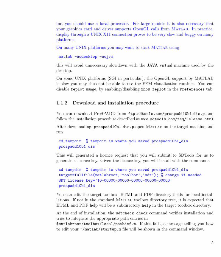
1.1.2 Download and installation procedure

You can download ProSPADD from ftp.sdtools.com/prospadd10b1 dis.p andfollow the installation procedure described at www.sdtools.com/faq/Release.html

After downloading, prospadd10b1 dis.p open Matlab on the target machine andrun

cd tempdir % tempdir is where you saved prospadd10b1_disprospadd10b1_dis

This will generated a licence request that you will submit to SDTools for us togenerate a licence key. Given the licence key, you will install with the commands

cd tempdir % tempdir is where you saved prospadd10b1_distarget=fullfile(matlabroot,’toolbox’,’sdt’); % change if neededSDT_license_key=’10-00000-00000-00000-00000-00000’prospadd10b1_dis

You can edit the target toolbox, HTML and PDF directory fields for local instal-lations. If not in the standard Matlab toolbox directory tree, it is expected thatHTML and PDF help will be a subdirectory help in the target toolbox directory.

At the end of installation, the sdtcheck check command verifies installation andtries to integrate the appropriate path entries in$matlabroot/toolbox/local/pathdef.m. If this fails, a message telling you howto edit your ~/matlab/startup.m file will be shown in the command window.

5

ftp://ftp.sdtools.com/prospadd10b1_dis.p

http://www.sdtools.com/faq/Release.html


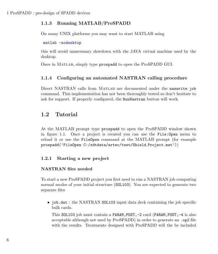
1.1.3 Running MATLAB/ProSPADD

On many UNIX platforms you may want to start MATLAB using

matlab -nodesktop

this will avoid unnecessary slowdown with the JAVA virtual machine used by thedesktop.

Once in Matlab, simply type prospadd to open the ProSPADD GUI.

1.1.4 Configuring an automated NASTRAN calling procedure

Direct NASTRAN calls from Matlab are documented under the naswrite jobcommand. This implementation has not been thoroughly tested so don’t hesitate toask for support. If properly configured, the RunNastran button will work.

1.2 Tutorial

At the MATLAB prompt type prospadd to open the ProSPADD window shownin figure 1.1. Once a project is created you can use the File:Open menu toreload it or use the FileOpen command at the MATLAB prompt (for exampleprospadd(’FileOpen C:/sdtdata/artec/test/Shield Project.mat’))

1.2.1 Starting a new project

NASTRAN files needed

To start a new ProSPADD project you first need to run a NASTRAN job computingnormal modes of your initial structure (SOL103). You are expected to generate twoseparate files

• job.dat : the NASTRAN SOL103 input data deck containing the job specificbulk cards.

This SOL103 job must contain a PARAM,POST,-2 card (PARAM,POST,-4 is alsoacceptable although not used by ProSPADD) in order to generate an .op2 filewith the results. Treatments designed with ProSPADD will the be included

6

by editing this initial file and generating a job Include.dat file that containsnew nodes, MPC and model matrices for the SPADD r© treatment.

Note that this job may refer to other files using include cards. These fileswill be copied to the solution directory when exporting a ProSPADD solutionto NASTRAN.

• job.op2 is the OUTPUT2 file generated when running job.dat. The file maybe generated on a system and read under any other operating system. If usingFTP for transfers, just make sure that the transfer is done in binary mode.

ProSPADD always uses the global coordinate system (basic coordinate system inNASTRAN terminology). Node locations are automatically transformed to thiscoordinate system when the model is loaded. The .op2 file does not however containinformation on which coordinate system was used for eigenvectors. If you havedeformations defined in a local coordinate system, use

pro=ApplyRule(’DefLocalToGlobal’,pro);

to transform your deformations to the global coordinate system. When reading amodel with local bases, you will be asked Do you need to transform deformationsto the global coordinate system ?. The answer depends on your NASTRAN config-uration.

7


Project files (Project tab File menu)

Figure 1.1: Project tab

To start a new project, start ProSPADD in Matlab then use the File:New menu,or click on the Name root area of the Project tab, or type prospadd(’FileNew’)at the Matlab prompt. This will open a dialog to let you select the job.dat orjob.op2 file which will be imported. The resulting model is saved in SDT formatin the job.mat file and project information is saved in job Project.mat.

When you write a solution (Placement:Write NASTRAN SOL menu), the currentstatus of your project (pro and sol variables) are saved in the solution directory(sol.wd) as a * Project.mat file. You can restart an analysis by loading this file.

Parameters for NASTRAN file ouput (Project tab)

In many cases you may want to tailor the identifiers used for the SPADD r© design.In particular, ProSPADD r© adds MPC constraints and nodes. In the project tab youcan thus specify

• MPC (set value) : the set identifier used for MPC constraints added to interpolateSPADD r© feet motion. (In script, set the pro.MPC value). When writting

8

ProSPADD solutions a MPC i card will be inserted before the BEGIN BULK andnew constraints will use pro.MPC as the SID value.

• NewNodeFrom : new node number to start from when defining new nodes duringProSPADD placement phases.

• Names which lets you modify the names attributed to matrices in NASTRANDMIG output generated by ProSPADD. In script, set the pro.MatrixNamescell array of names.

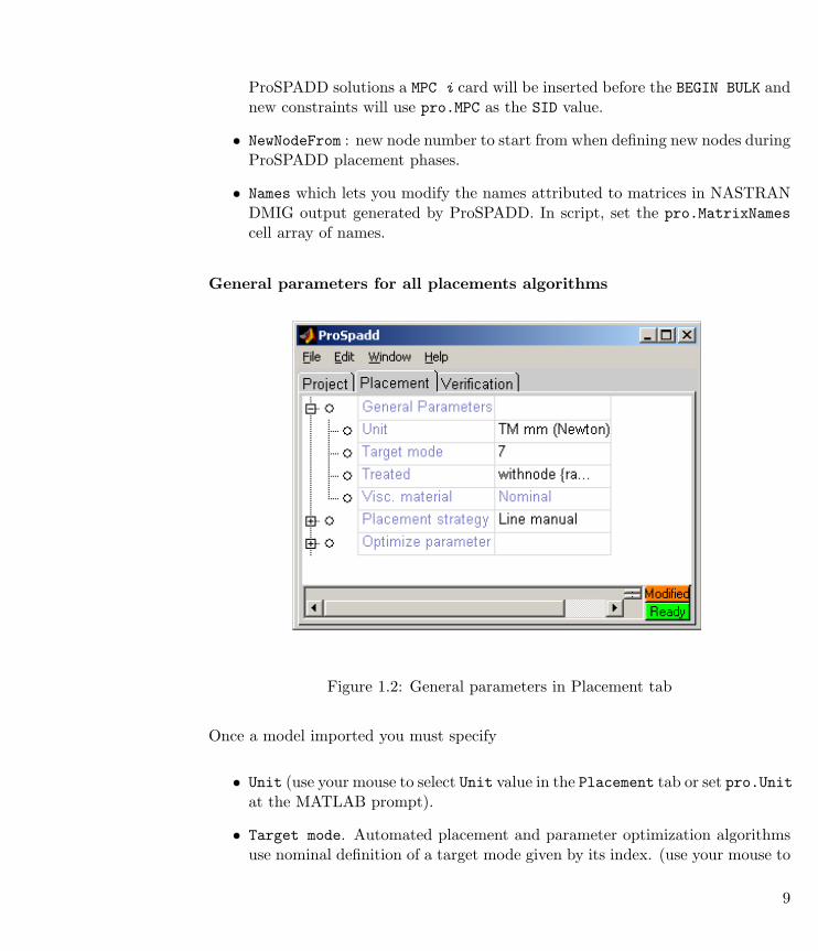
General parameters for all placements algorithms

Figure 1.2: General parameters in Placement tab

Once a model imported you must specify

• Unit (use your mouse to select Unit value in the Placement tab or set pro.Unitat the MATLAB prompt).

• Target mode. Automated placement and parameter optimization algorithmsuse nominal definition of a target mode given by its index. (use your mouse to

9


select Unit value in the Placement tab or set pro.TargMode=1 at the MAT-LAB prompt).

• Treated is the selection of the potential treatment area as detailed in sec-tion 1.2.1.

• Placement strategy is detailed in section 1.2.2. Currently implemented strate-gies allow for placement of struts, lineic devices and patches. In all cases youcan place a multiple treatments of the same type using the append versions ofthe strategy.

Potential treatment area

To place a device you first need to define a potential treatment area (by defaultpro.Treated=’GroupAll’ selects all elements). The potential treatment area is asurface declared through

• Elements with a given property identifier for example pro.Treated=’ProId1001:1004’

• Elements with a given material identifier for example pro.Treated=’MatId1001:1004’

• Node sets defined in the NASTRAN bulk file. For a SET entry placed in thecase control section (before the BEGIN BULK card), that will look like

SET 1 = 140443 THRU 140447,140457 THRU 140461,140471 THRU 140475,140485,140486 THRU 140489,140499,140500,140501,140502,140503

pro.Treated=’withnode {set 1}’ can be used to define the treated area.ID is the SET identification number in NASTRAN. The implementation of SETselection is fairly new, please report problems that may occur.

• Arbitrary selection of surfaces using the SDT node selection commands (usesdtweb(’findnode’) to find out more details). For example,

pro.Treated=’withnode {rad <=100 3.5 -6.12 5.2 & z>10 & z<100}’;

selects elements containing nodes within a radius of 100 of node 3.5 -6.125.2 and such that z>10 and z<100.

10

Warning : the potential treatment area must be fairly flat and the element normalsshould be nearly continuous. If the angle between the normals of two faces exceeds 25degrees, a warning is generated. The problem typically occurs when contiguous shellelements have opposite normals. This problem can be fixed using feutil orientcommands which are currently only available in script mode.

1.2.2 Device placement strategies

Point to point struts

Damped struts are simple point to point connections to account for the typicalphysical offset of the connection. They are modeled as 4 node connections

height

N

Figure 1.3: Parameters defining the geometry of the generic strut

Graphically, you can select the Point to Point placement strategy to define a newstrut. In script you will use a call of the form

prospadd(sprintf(’newstrut %i %i 30 0 1 0’,[node1 node2]));prospadd paroptim

where 30 is the strut height and 0 1 0 its orientation.

When optimizing multiple struts (Strut append strategy) a single stiffness value isused for all struts. To optimize multiple strut values, you need to run sequentialoptimizations (see section 1.2.4).

ProSPADD also provides an automated procedure to select the best in a seriesof struts. You must define a struts matrix where each row defines nodes to be

11


connected and an info matrix giving height and orientation for each strut (one perrow) or all struts (a single row). The call is then

opt=prospadd(’beststrut’,struts,info);

By default, the mass length rule for struts is defined by

setpref(’ProSpadd’,’StrutMassLaw’,’mass=(.865*L+1.5*L.\verb+^+2)’)

You can redefine this value if needed. Be careful that L is a vector so that the .^ isneeded.

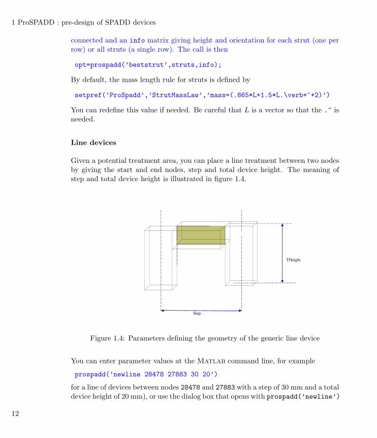
Line devices

Given a potential treatment area, you can place a line treatment between two nodesby giving the start and end nodes, step and total device height. The meaning ofstep and total device height is illustrated in figure 1.4.

Step

THeight

Figure 1.4: Parameters defining the geometry of the generic line device

You can enter parameter values at the Matlab command line, for example

prospadd(’newline 28478 27883 30 20’)

for a line of devices between nodes 28478 and 27883 with a step of 30 mm and a totaldevice height of 20 mm), or use the dialog box that opens with prospadd(’newline’)

12

or mouse selection of Line Manual in the Placement tab, Placement strategyvalue).

In script mode, you can place a new device line by providing the solution of anearlier placement in the command

prospadd(’newline NodeId1 NodeId2 Step THeight’,sol).

Once the device model created, you can directly optimize the viscoelastic stiffnessparameter (use prospadd(’paroptim’) or click on the run button in the OptimalKv entry.

You may want to run this optimization for different values of the foot thickness(lowering this value leads to weight saving but at some point the device framebecomes to flexible and the viscoelastic layer does not operate properly).

ProSPADD also provides an automated placement procedure of line devices. Beforeattempting an automated placement you must define

• Potential treatment area pro.Treated (this is a general parameter describedin section 3.1.5)

• Inter-foot step pro.Step as shown in figure 1.4.

• Maximum device height pro.THeight as shown in figure 1.4.

• Maximum number of patterns pro.MaxPat

• Target mode pro.TargMode

The placement of pro.MaxPat patterns is then made automatically with the com-mand prospadd(’place’) (or the associated button in the interface). To continueplacement of more patterns use prospadd(’place’,sol,pro). Note that you canalternate, manual and automated placement of line devices.

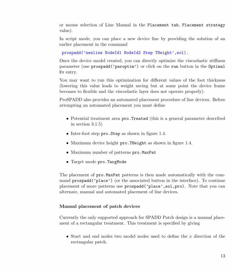
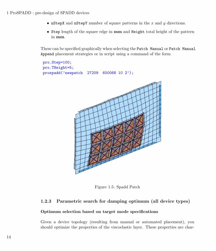
Manual placement of patch devices

Currently the only supported approach for SPADD Patch design is a manual place-ment of a rectangular treatment. This treatment is specified by giving

• Start and end nodes two model nodes used to define the x direction of therectangular patch.

13


• nStepX and nStepY number of square patterns in the x and y directions.

• Step length of the square edge in mm and Height total height of the patternin mm.

These can be specified graphically when selecting the Patch Manual or Patch ManualAppend placement strategies or in script using a command of the form

pro.Step=100;pro.THeight=5;prospadd(’newpatch 27209 600068 10 2’);

Figure 1.5: Spadd Patch

1.2.3 Parametric search for damping optimum (all device types)

Optimum selection based on target mode specifications

Given a device topology (resulting from manual or automated placement), youshould optimize the properties of the viscoelastic layer. These properties are char-

14

acterized by an equivalent stiffness. For SPADD-T and patches one uses a shearmodulus Kv in N/m, for struts one uses Kv/L in N/m2).

Running prospadd(’paroptim’) (Optimal kv button) generates a pole optimizationdisplay similar to that of figure 1.6. This graph shows the evolution of poles as afunction of kv. Poles at the optimal value are linked in red. Areas where the qualityof the estimation is doubtful are shown in grey.

620 640 660 680 700 720 7400

0.5

1

1.5

2

2.5

3

3.5

Frequency

ζ =1.89 %

kV=8.7e+005 N/m

Madd

= 8.71 gD

ampi

ng r

atio

%

Figure 1.6: Parametric optimization pole display.

You can modify the optimum retained for the validation steps by clicking on thedesired location of the pole display or rerun an optimization near a particular valuegiven in the paroptim command (for example prospadd(’paroptim 1e4’)).

Optimum selection based target transfer specifications

Target transfers are evaluated by ProSPADD when inputs, outputs and frequenciesare specified. The show button sets default inputs and outputs at the DOF with thelargest response and a frequency range that spans the given modal basis.

Target transfer specification in the NASTRAN bulk is not currently tested. So youmay need to reenter the appropriate values.

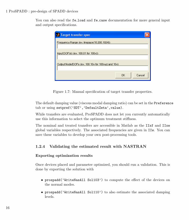
When clicking on the target transfer button the dialog in figure 1.7, lets you specify afrequency range (using any Matlab command), the input DOF(s) (using standardSDT DOF specification 1.01 for 1x 1 for inputs in all three directions, for moredetails see sdtweb(’adof’)), the output DOFs (list of DOFs or node numbers,when given node numbers all translations are retained).

15


You can also read the fe load and fe case documentation for more general inputand output specifications.

Figure 1.7: Manual specification of target transfer properties.

The default damping value (viscous modal damping ratio) can be set in the Preferencetab or using setpref(’SDT’,’DefaultZeta’,value).

While transfers are evaluated, ProSPADD does not let you currently automaticallyuse this information to select the optimum treatment stiffness.

The nominal and treated transfers are accessible in Matlab as the IIxf and IIxeglobal variables respectively. The associated frequencies are given in IIw. You cansave these variables to develop your own post-processing tools.

1.2.4 Validating the estimated result with NASTRAN

Exporting optimization results

Once devices placed and parameter optimized, you should run a validation. This isdone by exporting the solution with

• prospadd(’WriteNasAll Sol103’) to compute the effect of the devices onthe normal modes.

• prospadd(’WriteNasAll Sol110’) to also estimate the associated dampinglevels.

16

The solution is saved in the directory given in sol.wd (the default for that directoryis fullfile(pro.Files.wd,[pro.Files.root ’ Solution1’]) ). Files saved inthe directory are

• job sol1xx.dat a copy of the original bulk file (and copies of any includefile) with modifications to specify included matrices, etc. For sol110 thisincludes DMAP alter cards to include hysteretic damping of the devices as aK4GG matrix (note that this DMAP alter currently only works with NASTRAN2001 and 2004, you can select the target version using

setpref(’FEMLink’,’NASTRAN’,2001)}).

Note that manual name assignments such as

ASSIGN OUTPUT2 = ’p1\_seule.op2’, UNIT = 12

are not modified. You are thus expected to verify and possibly edit thejob sol1xx.dat file before actually running it.

• job Include.dat contains the device superelement representation and as com-ments the current state of ProSPADD when the solution is written

• sol.mat containing the pro and sol variables when the include is generated.

SOL110 is used for the final validation run with the reference NASTRAN approach.SOL103 is used during validations of the solution with damping being estimated byProSPADD.

Using the new NASTRAN result for reoptimization

Reoptimization near the value obtained after a SOL103 run is done as follows

1. in the initial design (Placement tab), generate a SOL103 using the WriteNASTRAN SOL button.

2. Run NASTRAN and place the resulting job sol103.op2 file in the directorywhere the initial design was saved (the location of this directory is given insol.wd).

3. Go to the verification tab and click on the Import SOL103 button. ProSPADDwill then show information similar to that in figure 1.8.

17


4. Clicking on the Current K v button reruns a parameter optimization near thestarting value used for the NASTRAN run. The value shown in red in thepole display (see figure 1.6) corresponds to this nominal value. You can thenselect other points on the display and restart an cycle (step 1 but now WriteNASTRAN SOL button in the Verification tab.

ss

Figure 1.8: Verification tab.

Sequential optimization

Sequential optimization is the process of using the result of a ProSPADD run torestart a new project that retains previously placed/optimized SPADD treatments.The validity of the associated approximations are discussed in Ref. [?].

1.3 Principles of placement algorithms

1.3.1 Topology search

The placement algorithm is a two step process where one first builds a map ofefficient locations for viscoelastic treatments then optimally places devices on theavailable structure based on the efficiency map.

Starting from the model of the supporting structure. One defines

• the potential treatment area (specified using the element selection stringpro.Treated and shown in blue in the figure, see more details in section 1.2.1).

18

The potential treatment is a combination of surfaces (shells or volume faces)that are relatively flat (angle between normals of contiguous elements less than5 degrees).

• working height for the viscoelastic material. This height corresponds to themiddle of the viscoelastic layer. The actual device height (parameter pro.THeight)is thus higher by half the height of the viscoelastic layer.

Figure 1.9: Selection of the potential treatment area.

One then computes at the strain field of a membrane placed at the working heightfrom the surface of the potential treatment area. For each computed mode, the prin-cipal strain with the largest absolute value gives a direct indication of the dampingpotential for a pattern that would be placed on the element, and the associatedprincipal direction gives the optimal pattern direction. This computation can beused to generate vector fields of damping potential as shown in figure 1.10.

19


1 @ 621.8 Hz

Figure 1.10: Damping potential map : Vector field associated to principal membranestrains for mode 1.

Given the damping potential map, the placement algorithm uses the additionalparameters

• pro.MindDist : minimum inter-foot distance (default value pro.Height*2/3)

• pro.TargMode : index of target mode considered for the placement

• pro.Step : distance between pattern foot nodes

• pro.MaxPat : maximum number of patterns to be placed by the algorithm

• pro.MaxPatternAngle : maximum angle between to successive patterns (angleon the available surface and not variation between normals on the surface).Manufacturing constraints usually impose that this be set to zero.

and works as follows

1. Start a new device

• Within the available remaining element list (initialized to the full poten-tial treatment area) select the element with maximum potential.

• Place the first foot at the element node that has the best average potential(mean potential of neighboring elements) but favoring nodes that are noton the surface edge.

20

• Use the direction of the principal strain as the device direction

2. Append patterns to a device

• Compute the position of foots for patterns placed at the head or tail ofthe current device

• Determine the damping potential of each possible pattern by finding theelement associated with their feet and looking up associated the principalmembrane strain.

• Add the pattern with the maximum potential.

• Update the direction for tail/head addition of a new pattern. The nominalnew direction is the direction of the principal strain. However, if the anglebetween that direction and the direction of the preceding pattern is higherthan pro.MaxPatternAngle one rotates the earlier direction towards theprincipal strain direction by pro.MaxPatternAngle.

• Eliminate elements with at least one node within pro.MindDist from theadditional foot from the remaining element list.

3. Test for the need to start a new device

• If the potential foot location is outside the potential treatment area, stopadding patterns to this end of the device

• If the principal strain associated with a given foot location is less than 50

• If the desired number of patterns is reached, stop the placement algo-rithm.

4. Format placement algorithm output.

• Build a series multiple point constrains MPC to interpolate the displace-ment of device feet that do not coincide with nodes of the original mesh.

• Build a simplified representation of the devices. Xxx distinguish displayand computations xxx

During the placement phase, placed feet and the remaining element list are displayed.The resulting devices can be displayed as shown in figure 1.11. Note in the figurethat the deformation of the devices is computed based on the modes of the nominaluntreated model.

21


1 @ 621.8 Hz

Figure 1.11: Nominal mode shape with deformations of the newly placed devices.

1.3.2 Parameter optimization algorithm

The parameter optimization algorithm uses the following procedure

1. building of a generic superelement SE representing the pattern information.This superelement is expected to have one parameter that will be varied. Cur-rently, SE building is implemented for struts, the T and patch patterns.

2. Given the superelement representation of the pattern, the placement solutionsol (see previous section) and nominal deformations, one computes poles ofthe reduced model for a range of parameter values (100 points from 10-4 to 100times the nominal value), leading to the pole display below where the value ofthe optimum for the target mode is shown.

22

620 640 660 680 700 720 7400

0.5

1

1.5

2

2.5

3

3.5

Frequency

ζ =1.89 %

kV=8.7e+005 N/m

Madd

= 8.71 g

Dam

ping

rat

io %

Figure 1.12: Parametric optimization pole display.

1.3.3 Validation of design result

In this phase one exports to NASTRAN bulk format of a model of the design result(this bulk is appended to the original model using an include card). This can thenbe used to validate the optimization results by running a complex mode analysis(SOL 107 (direct), SOL110 (modal)) or direct frequency response (SOL 108).

1.4 Reference information

1.4.1 pro and sol data structures

Most of ProSPADD information is stored in the pro data structure with the followingfields.

23


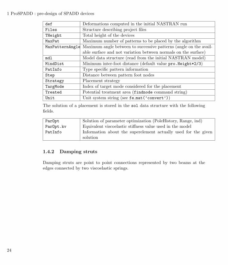
def Deformations computed in the initial NASTRAN runFiles Structure describing project filesTHeight Total height of the devicesMaxPat Maximum number of patterns to be placed by the algorithmMaxPatternAngle Maximum angle between to successive patterns (angle on the avail-

able surface and not variation between normals on the surface)mdl Model data structure (read from the initial NASTRAN model)MindDist Minimum inter-foot distance (default value pro.Height*2/3)PatInfo Type specific pattern informationStep Distance between pattern foot nodesStrategy Placement strategyTargMode Index of target mode considered for the placementTreated Potential treatment area (findnode command string)Unit Unit system string (see fe mat(’convert’))

The solution of a placement is stored in the sol data structure with the followingfields.

ParOpt Solution of parameter optimization (PoleHistory, Range, ind)ParOpt.kv Equivalent viscoelastic stiffness value used in the modelPatInfo Information about the superelement actually used for the given

solution

1.4.2 Damping struts

Damping struts are point to point connections represented by two beams at theedges connected by two viscoelastic springs.

24

height

N

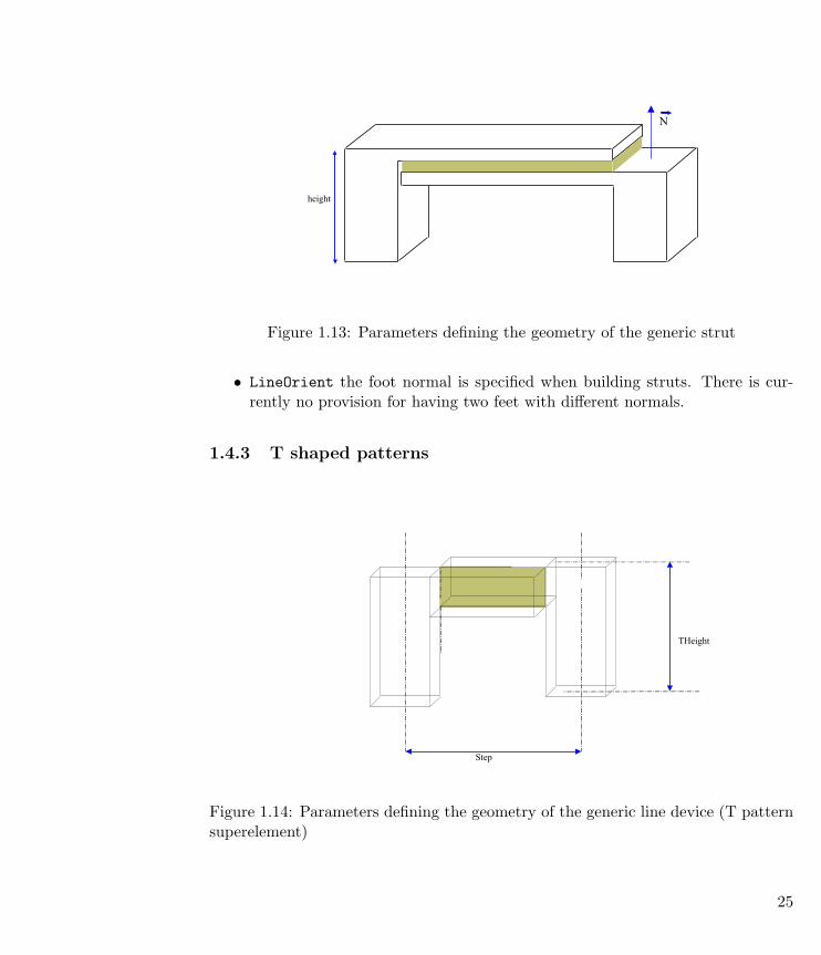
Figure 1.13: Parameters defining the geometry of the generic strut

• LineOrient the foot normal is specified when building struts. There is cur-rently no provision for having two feet with different normals.

1.4.3 T shaped patterns

Step

THeight

Figure 1.14: Parameters defining the geometry of the generic line device (T patternsuperelement)

25


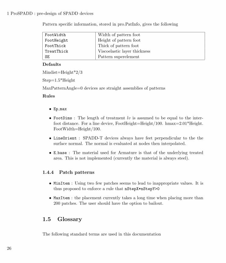
Pattern specific information, stored in pro.PatInfo, gives the following

FootWidth Width of pattern footFootHeight Height of pattern footFootThick Thick of pattern footTreatThick Viscoelastic layer thicknessSE Pattern superelement

Defaults

Mindist=Height*2/3

Step=1.5*Height

MaxPatternAngle=0 devices are straight assemblies of patterns

Rules

• Ep max

• FootDims : The length of treatment lv is assumed to be equal to the inter-foot distance. For a line device, FootHeight=Height/100. hmax=2.01*Height.FootWidth=Height/100.

• LineOrient : SPADD-T devices always have feet perpendicular to the thesurface normal. The normal is evaluated at nodes then interpolated.

• E base : The material used for Armature is that of the underlying treatedarea. This is not implemented (currently the material is always steel).

1.4.4 Patch patterns

• MinItem : Using two few patches seems to lead to inappropriate values. It isthus proposed to enforce a rule that nStepX*nStepY>0

• MaxItem : the placement currently takes a long time when placing more than200 patches. The user should have the option to bailout.

1.5 Glossary

The following standard terms are used in this documentation

26

Foil ClinquantDevice DispositifPattern MotifStrut TirantTopology search Recherche topologiqueDiscrete search Recherche discretreFrame Armature

1.6 Common problems

• You must set units ... when reading the model initially ProSPADD setspro.Unit=’US’ (for user coherent unit system). To allow placement you mustset the unit system in tab Placement:General Parameters:Unit or in theMatlab command line.

• File does not contain BEGIN BULK ProSPADD writes its solution by edit-ing a NASTRAN job file that is valid on your system. When starting a newproject, it is thus essential that the bulk file you select contains the full joband not just the model definition (bulk part. Failure to do so limits the abilityof ProSPADD to write solutions in the form of NASTRAN bulks.

• Model in file.mat does not define deformations the .op2 file where themodes are saved needs to contain normal mode shapes. Omitting the DISP=ALL card or equivalent in the job file is a usual reason for generating .op2 fileswithout deformations.

• Discontinuous treated area. When using automated placement, you arenot supposed to use treated areas that are segmented in more than one sur-face because : there is a discontinuity in the normal field; because the area issegmented in more than one piece. ProSPADD gives a warning in such situa-tions (”area segmented”) but tries to pursue. You are supposed to judgethe validity of results obtained in such cases by yourself.

• Problems with visualizing deformations. On some UNIX platforms, thevisualization of FEM meshes can cause MATLAB to be very slow or even crash.This is due to know problems with how Matlab calls OpenGL libraries.

You can avoid displaying deformations by setting

setpref(’ProSpadd’, ’feplot’,0)

27


which is also available in the Preference tab. You can also avoid callingOpenGL by including the following command in your startup file

sdtdef(’DefaultFeplot’,{’Renderer’ ’zbuffer’ ...’doublebuffer’ ’on’})

28

ProSpadd - · PDF file1.2 Tutorial ... will be copied to the solution directory when...

Documents

Transcript of ProSpadd - · PDF file1.2 Tutorial ... will be copied to the solution directory when...