Cover Sheet for Presentation to IEEE 802.16 Broadband Wireless Access Working Group (Rev. 0)

Document Number:IEEE 802.16.1pp-00/15

Title:

Proposed System Impairment ModelsDate Submitted: 2000-03-08Source:

John Liebetreu Voice: 408-607-4830Sicom Inc. Fax: 408-607-4806785 East Redfield Road E-mail: john@sicom.comScottsdale, Arizona 85260

Co-presenters: David Falconer, Carleton University, Tom Kolze, Broadcom, Yigal Leiba, BreezecomVenue:

IEEE 802.16 meeting, Albuquerque, NM, March 6-10, 2000Base Document:

802.16.1pc-00/15 http://ieee802.org/16/phy/docs/802161pc-00_15.pdfPurpose:

Aid in the PHY Task Group’s preparation of a detailed evaluation table for performance of PHY layer air interface proposals.Notice:

This document has been prepared to assist the IEEE 802.16. It is offered as a basis for discussion and is not binding on the contributingindividual(s) or organization(s). The material in this document is subject to change in form and content after further study. Thecontributor(s) reserve(s) the right to add, amend or withdraw material contained herein.

Release:The contributor acknowledges and accepts that this contribution may be made public by 802.16.

IEEE Patent Policy:

The contributor is familiar with the IEEE Patent Policy, which is set forth in the IEEE-SA Standards Board Bylaws<http://standards.ieee.org/guides/bylaws> and includes the statement: “IEEE standards may include the known use of patent(s),including patent applications, if there is technical justification in the opinion of the standards-developing committee and provided theIEEE receives assurance from the patent holder that it will license applicants under reasonable terms and conditions for the purpose ofimplementing the standard.”

System Impairment Model

Ad hoc modelling committee:

David Falconer, Carleton University

Tom Kolze, Broadcom

Yigal Leiba, Breezecom

John Liebetreu, Sicom

With thanks also to:Naftali Chayat, (Breezecom) Bruce Cochran, (Sicom) Scott Enserink, (Sicom)

Lucille Rouault, (ENST/NIST) Val Rhodes, (Intel) Benoit Verbaere,(ENST/NIST)

Process

• Identify primary performance degradationsources

• Model and parameterize these sources

• Establish performance metrics

• Establish baseline characterizationtechniques

Performance degradation sources

• Phase noise

• Power amplifier

• Multi-path

• Model parameters may be– Set by group and simulated by contributors

– Stated and simulated by contributors

Power Amplifier Models

Saleh Model• Uses simple two-parameter functions to model

the AM-to-PM and AM-to-AM characteristics ofnonlinear amplifiers.

• Originally developed to specify the behavior ofTWTA’s. Appropriate selections for theamplitude and phase coefficients (α’s and β’s)provide a suitable model for solid stateamplifiers as well.

• It is a frequency-independent model. Can bemade frequency-dependent by adding filters thatmirror how the coefficients change withfrequency.

Saleh ModelInput signal:

x(t)=r(t)cos[ω0t+ψ(t)]• ω0 is the carrier frequency,

• r(t) is the modulated envelope• ψ(t) is the modulated phase

The output of the nonlinear amplifier is:y(t)=A[r(t)]cos{ω0t+ψ(t)+Φ(r(t))}

• A(r) represents the AM-to-AM conversion• Φ(r) represents the AM-to-PM conversion.

Saleh Model• The specific forms of the two functions:

A(r)=αar/(1+βar2)

Φ(r)=αφr2/(1+βφr

2)

• As an example, the set of parameters thatclosely matches TWTA data [1] is,

αa= 2.1587 βa= 1.1517

αφ= 4.033 βφ= 9.1040

Saleh Model

Kaye, George, and Eric

0

0.2

0.4

0.6

0.8

1

1.2

0 0.2 0.4 0.6 0.8 1 1.2 1.4 1.6 1.8 2

Input Amplitude

Ou

tpu

t A

mp

litu

de

0

10

20

30

40

50

60

70

80

90

Ou

tpu

t P

ha

se

(d

eg

)

AM-AM AM-PM

Saleh model with parameters:αa= 2.1587, βa= 1.1517, αφ= 4.033, βφ= 9.1040

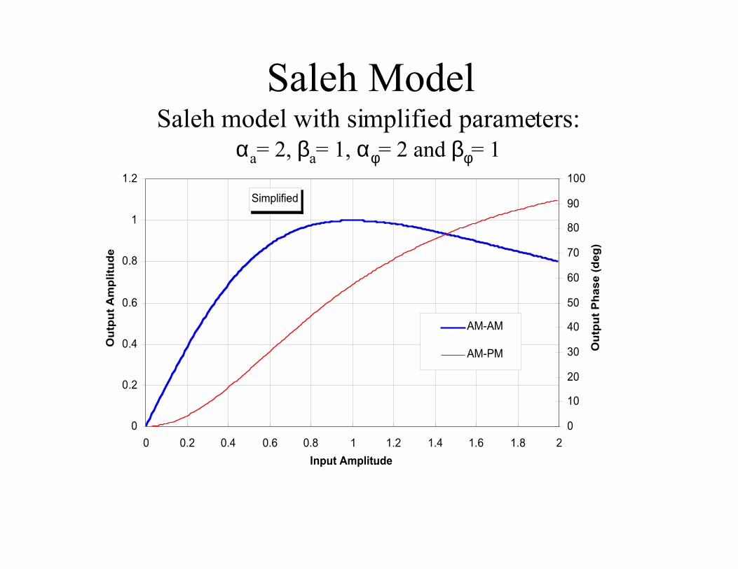
Saleh ModelSaleh model with simplified parameters:

αa= 2, βa= 1, αφ= 2 and βφ= 1

Simplified

0

0.2

0.4

0.6

0.8

1

1.2

0 0.2 0.4 0.6 0.8 1 1.2 1.4 1.6 1.8 2

Input Amplitude

Ou

tpu

t A

mp

litu

de

0

10

20

30

40

50

60

70

80

90

100

Ou

tpu

t P

ha

se

(d

eg

)

AM-AM

AM-PM

Saleh Model Summary

• Uses simple two-parameter functions to model theAM-to-PM and AM-to-AM characteristics ofnonlinear amplifiers.

• Appropriate selections for the amplitude and phasecoefficients (α’s and β’s) can provide a suitablemodel for solid state amplifiers well.

• Saleh’s models for TWTAs are shown toaccurately match actual measured data .

• Can be altered to a frequency-dependent model.

Rapp Model

• Developed for solid-state power amplifiers.• Produces a smooth transition for the

envelope characteristic as the inputamplitude approaches saturation.

Vout = Vin/(1 + (|Vin|/Vsat)2P)1/(2P)

Where Vsat is the saturation voltage of thepower amplifier and P is the smoothnessfactor.

Rapp ModelCurves for various smoothness factors “P”:

Output Amplitude vs. Input Amplitude for Rapp Model of HPA

0

0.2

0.4

0.6

0.8

1

1.2

0 0.2 0.4 0.6 0.8 1 1.2 1.4 1.6 1.8 2

Normalized Input Amplitude

Ou

tpu

t A

mp

litu

de

P = 100

P = 10

P = 2.0

P = 1.0

P = 0.5

Rapp Model- Modified• Honkanen and Haggman altered the low-level

portion of the AM/AM characteristic in order tobetter mirror the exponential relationships of bipolarjunction devices.

• Included AM/PM model as well.• Their AM/AM and AM/PM models matched

measurements of actual class AB mobile phoneamplifier.

• Resulted in more accurate portrayal ofintermodulation effects than the Rapp model whencompared to a class AB mobile phone amplifier.

• They do not list their model’s parameters.

Ghorbani model• Similar approach to Saleh.• Claimed more suitable for SSPAs then Saleh.• PA output :

y(t)=A(r(t))cos{ω0t+Ψ(t)+Φ(r(t))}where,A(r) = x1rx2/(1+x3rx2) + x4rΦ(r) = y1ry2/(1+y3ry2) + y4r

• For the GaAs FET SSPA characterized by Ghorbani:

x1 = 8.1081 y1 = 4.6645x2 = 1.5413 y2 = 2.0965x3 = 6.5202 y3 = 10.88x4 = -0.0718 y4 = -0.003

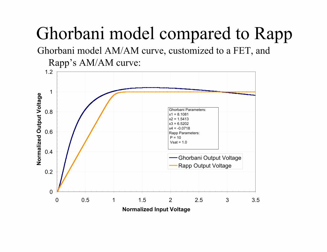
Ghorbani model compared to RappGhorbani model AM/AM curve, customized to a FET, and

Rapp’s AM/AM curve:

0

0.2

0.4

0.6

0.8

1

1.2

0 0.5 1 1.5 2 2.5 3 3.5

Normalized Input Voltage

No

rmal

ized

Ou

tpu

t V

olt

age

Ghorbani Output VoltageRapp Output Voltage

Ghorbani Parameters:x1 = 8.1081x2 = 1.5413x3 = 6.5202x4 = -0.0718Rapp Parameters: P = 10 Vsat = 1.0

Ghorbani Compared to SalehGhorbani model AM/AM curve, customized to a FET, and

Saleh model’s best fit to that curve:

0

0.2

0.4

0.6

0.8

1

1.2

0 0.5 1 1.5 2 2.5 3 3.5

Normalized Input Voltage

No

rmal

ized

Ou

tpu

t V

olt

age

Ghorbani Output VoltageSaleh Output Voltage

Ghorbani Parameters:x1 = 8.1081x2 = 1.5413x3 = 6.5202x4 = -0.0718Saleh Parameters: α = 1.3325β = 0.3403

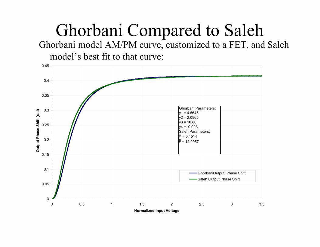
Ghorbani Compared to SalehGhorbani model AM/PM curve, customized to a FET, and Saleh

model’s best fit to that curve:

0

0.05

0.1

0.15

0.2

0.25

0.3

0.35

0.4

0.45

0 0.5 1 1.5 2 2.5 3 3.5

Normalized Input Voltage

Ou

tpu

t P

has

e S

hif

t (r

ad)

GhorbaniOutput Phase Shift

Saleh Output Phase Shift

Ghorbani Parameters:y1 = 4.6645y2 = 2.0965y3 = 10.88y4 = -0.003Saleh Parameters: α = 5.4514β = 12.9957

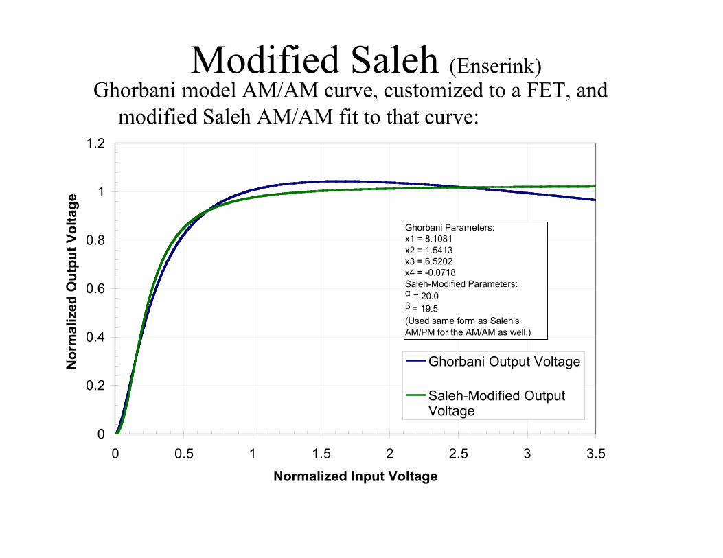
Modified Saleh (Enserink)

0

0.2

0.4

0.6

0.8

1

1.2

0 0.5 1 1.5 2 2.5 3 3.5

Normalized Input Voltage

No

rmal

ized

Ou

tpu

t V

olt

age

Ghorbani Output Voltage

Saleh-Modified OutputVoltage

Ghorbani Parameters:x1 = 8.1081x2 = 1.5413x3 = 6.5202x4 = -0.0718Saleh-Modified Parameters: α = 20.0β = 19.5(Used same form as Saleh's AM/PM for the AM/AM as well.)

Ghorbani model AM/AM curve, customized to a FET, andmodified Saleh AM/AM fit to that curve:

Ghorbani Compared to Saleh

• Saleh model matches the GaAs FET amplifier’sAM/PM characteristic well.

• Saleh model does not match the FET amplifier’sAM/AM characteristic very well. Can improve thematch by changing the Saleh AM/AM equation tohave the same form as the Saleh AM/PM equation.

• Ghorbani model is better suited to the FETamplifier’s characteristics and matches them closely.

Recommendation

• Adopt the well-known Saleh model as acomparison baseline.

• Baseline model serves as a reference pointfor comparison with other power amplifiermodels, (e.g., Ghorbani model).

References

• A.A.M. Saleh, “Frequency-independent and frequency-dependent nonlinear models ofTWT amplifiers,” IEEE Trans. Communications, vol. COM-29, pp.1715-1720,November 1981.

• A.R. Kaye, D.A. George, and M.J. Eric, “Analysis and compensation of bandpassnonlinearities for communications,” IEEE Trans. Communications Technology, vol.COM-20, pp.965-972, October 1972

• C. Rapp, “Effects of HPA-Nonlinearity on a 4-DPSK/OFDM-Signal for a DigitialSound Broadcasting System”, in Proceedings of the Second European Conference onSatellite Communications, Liege, Belgium, Oct. 22-24, 1991, pp. 179-184.

• M. Honkanen and Sven-Gustav Haggman, “New Aspects on Nonlinear PowerAmplifier Modeling in Radio Communication System Simulations”, Proc. IEEE Int.Symp. On Personal, Indoor, and Mobile Comm.,PIMRC ’97, Helsinki, Finland, Sep.1-4, 1997, pp. 844-848.

• A. Ghorbani, and M. Sheikhan, “The effect of Solid State Power Amplifiers (SSPAs)Nonlinearities on MPSK and M-QAM Signal Transmission”, Sixth Int’l Conferenceon Digital Processing of Signals in Comm., 1991, pp. 193-197.

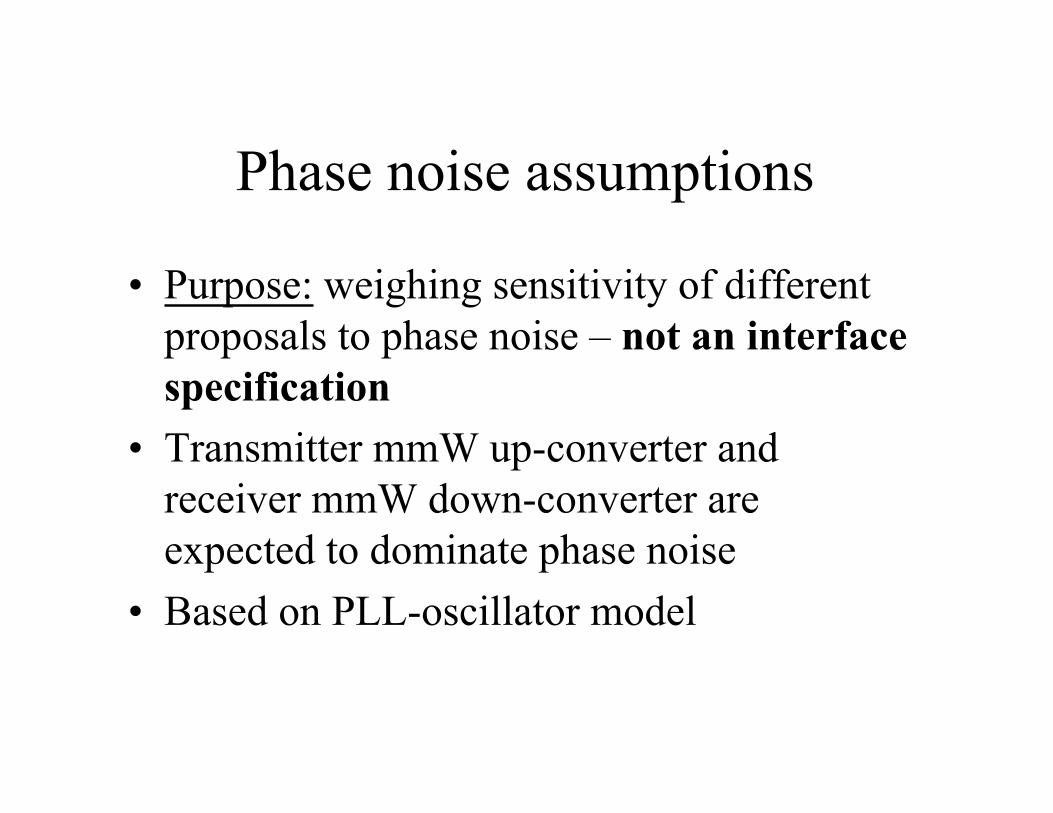
Phase noise assumptions

• Purpose: weighing sensitivity of differentproposals to phase noise – not an interfacespecification

• Transmitter mmW up-converter andreceiver mmW down-converter areexpected to dominate phase noise

• Based on PLL-oscillator model

SSB phase noise PSD, L(f)

log(f)

log(PSD)

fxtal floop

Lfloor

Lloop

20dB/dec

20dB/dec

20dB/dec

100MHz1Hz

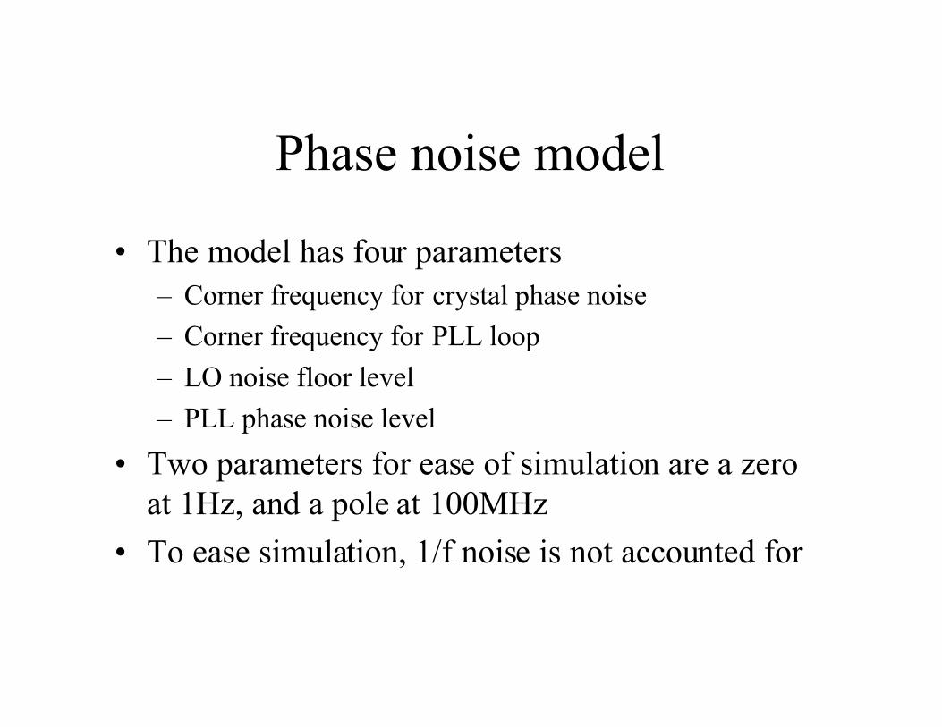
Phase noise model

• The model has four parameters– Corner frequency for crystal phase noise

– Corner frequency for PLL loop

– LO noise floor level

– PLL phase noise level

• Two parameters for ease of simulation are a zeroat 1Hz, and a pole at 100MHz

• To ease simulation, 1/f noise is not accounted for

Phase noise notes

• Thermal noise, discrete spurs anddemodulator induced phase noise are NOTincluded in this model.

• Model is to be used for comparisonpurposes, NOT for precise performanceevaluation

ETSI/BRAN Multipath Models ETSI/BRAN document HAPHY151TL03, “Channel model suitable for bands over 20 GHz”,

21 Sept. 1999.

0 40 ns.

0.96

-0.19

0 40 ns.

0.96

0.19exp(-jφ)

T1: T2:

ϕ=π(1-0.8(40 ns.)/Tsymbol))

Based on measurements in Europe by Telia

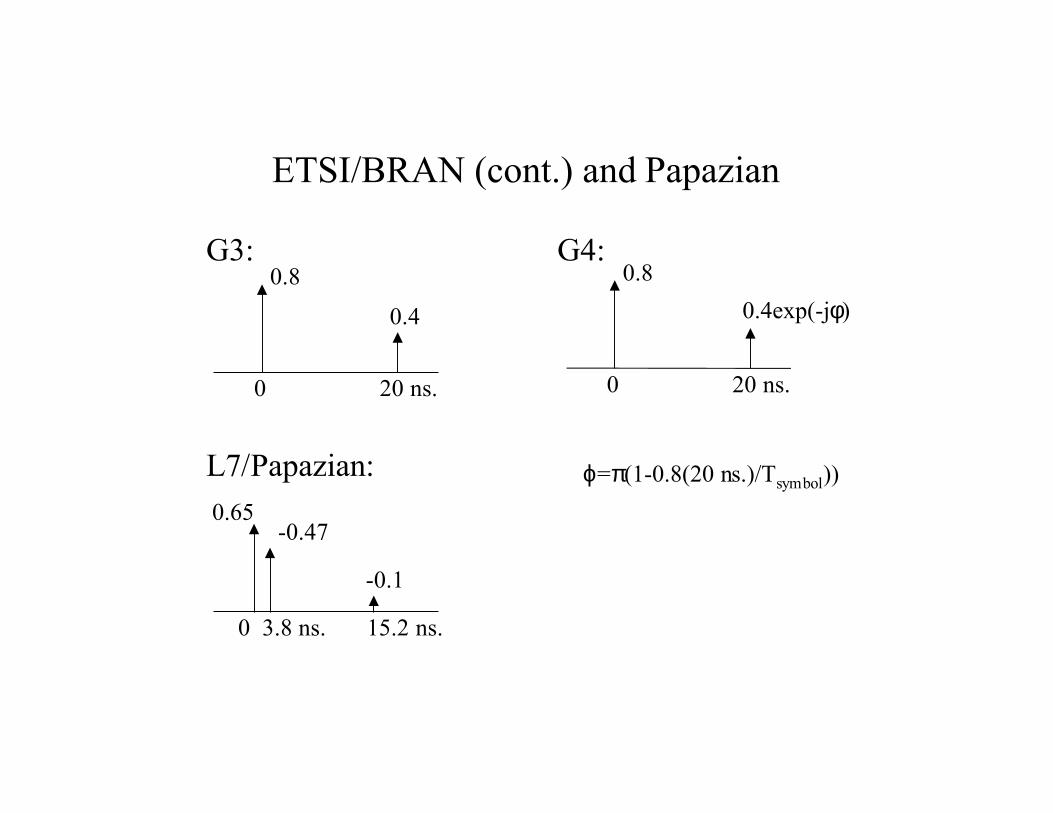
ETSI/BRAN (cont.) and Papazian

0 20 ns.

0.8

0.4

0 20 ns.

0.8

0.4exp(-jφ)

ϕ=π(1-0.8(20 ns.)/Tsymbol))

G3: G4:

0.65

-0.1

0 3.8 ns. 15.2 ns.

L7/Papazian:

-0.47

Some Measured Kanata Responses

-100 -80 -60 -40 -20 0 20 40 60 80 1000

0.1

0.2

0.3

0.4

0.5

0.6

0.7

Time (ns.)

Response magnitude

Kanata channel kab23002

-100 -80 -60 -40 -20 0 20 40 60 80 1000

0.1

0.2

0.3

0.4

0.5

0.6

0.7

Time (ns.)

Response magnitude

Kanata channel kgb30044

-100 -80 -60 -40 -20 0 20 40 60 80 1000

0.1

0.2

0.3

0.4

0.5

0.6

0.7

Time (ns.)

Response magnitude

Kanata channel kab23031

-100 -80 -60 -40 -20 0 20 40 60 80 1000

0.1

0.2

0.3

0.4

0.5

0.6

0.7

Time (ns.)

Response magnitude

Kanata channel kab29069

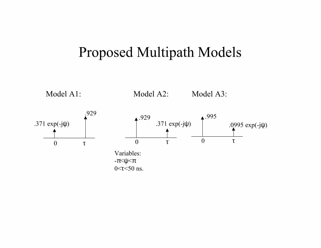
Proposed Multipath Models

0 τ

.929.371 exp(-jψ)

0 τ

.371 exp(-jψ)

.929

Variables:-π<ψ<π0<τ<50 ns.

0 τ

.995.0995 exp(-jψ)

Model A1: Model A2: Model A3:

Proposed Multipath Models (cont.)

Time variation? -- slow compared to symbol rate

.908

-0.279 0.279 exp(-jψ) -0.140

-20 ns. 0 20 ns. 50 ns.

Variable: -π<ψ<π

Model B:

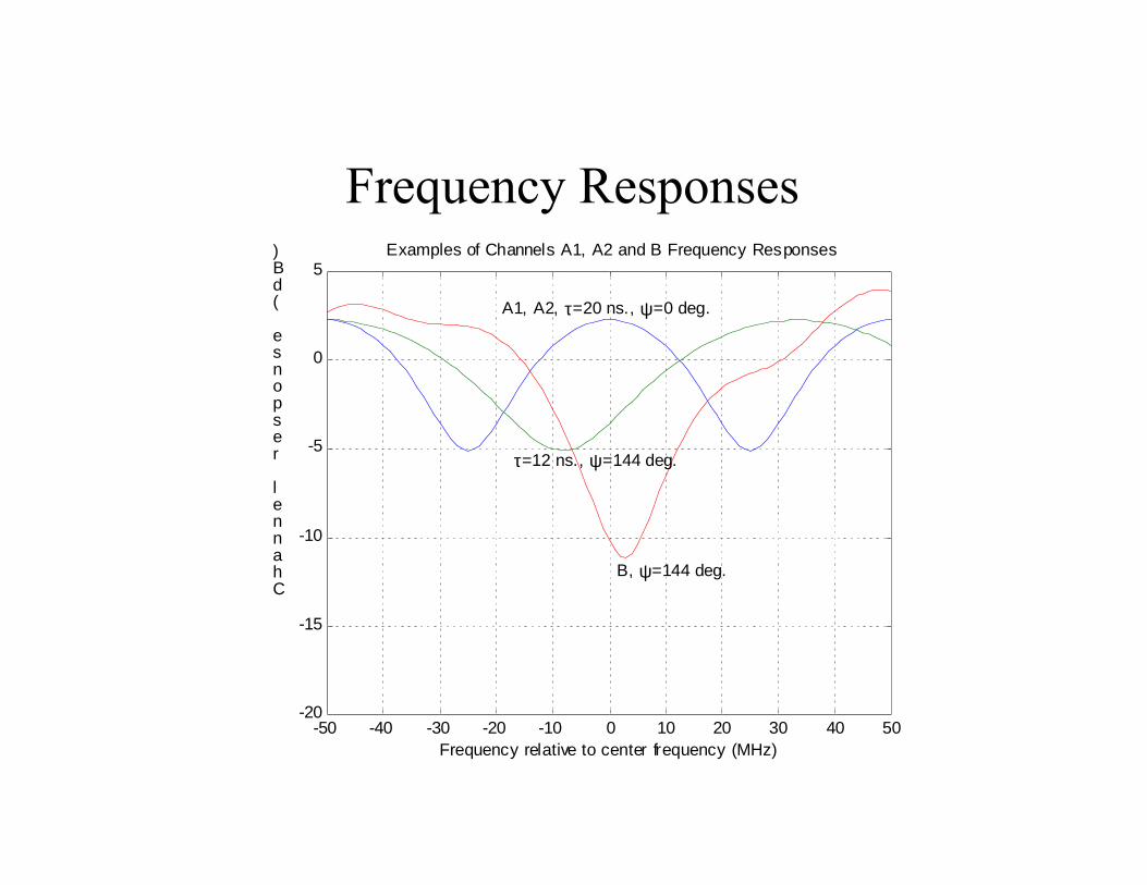
Frequency Responses

-50 -40 -30 -20 -10 0 10 20 30 40 50-20

-15

-10

-5

0

5

Frequency relative to center frequency (MHz)

Channel response (dB) Examples of Channels A1, A2 and B Frequency Responses

A1, A2, τ=20 ns., ψ=0 deg.

τ=12 ns., ψ=144 deg.

B, ψ=144 deg.

SNR Degradation for (8,1) DFE(50 Megasymbols/s)

0

1

2

3

4

5

6

7

0 45 90 135 180

Phase shift (degrees)

SNR degradation

(dB)

MODEL A1MODEL A2MODEL B

SNR Degradation for (8,1) DFE(25 Megasymbols/s)

-2

-1

01

2

3

4

5

6

7

0 45 90 135 180

Phase shift (degrees )

SNR degradation

(dB)

MODEL A1MODEL A2MODEL B

Conclusions on Multipath Modeling

• Three 2-tap and one 3-tap models proposed for PHYevaluation purposes, with variable phase and delayparameters.

• “Worst case” channels, including some with precursors(non-minimum phase). Examples of equalizer performance(not optimized).

• Fairly consistent with others’ models in terms of delayspread and echo magnitudes.