Proportional/Integral/DerivativeProportional/Integral/DerivativeControlControl

The PID instruction is an output instruction that controls physical properties such as temperature, pressure, liquid level, or flow rate using process loops.

PID ConceptPID Concept

The PID instruction normally controls a closed loop using inputs from an analog input module and providing an output to an analog output module. For temperature control, you can convert the analog output to a time proportioning on/off output for driving a heater or cooling unit.

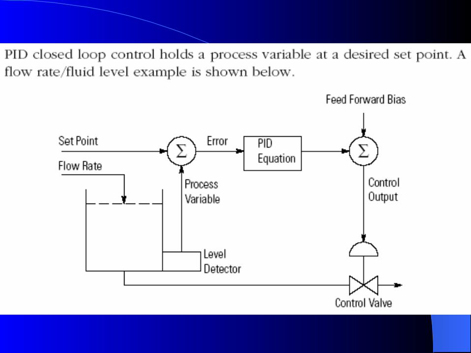
PID ControlPID ControlThe PID equation controls the process by sending

an output signal to the control valve. The greater the error between the setpoint and process variable input, the greater the output signal. Alternately, the smaller the error, the smaller the output signal. An additional value (feed forward or bias) can be added to the control output as an offset. The PID result (control variable) drives the process variable toward the set point.

PID EquationPID Equation

PID DIAGRAMPID DIAGRAM

Control system performance is often measured by applying a step function as the set point command variable, and then measuring the response of the process variable. Commonly, the response is quantified by measuring defined waveform characteristics. Rise Time is the amount of time the system takes to go from 10% to 90% of the steady-state, or final, value. Percent Overshoot is the amount that the process variable overshoots the final value, expressed as a percentage of the final value. Settling time is the time required for the process variable to settle to within a certain percentage (commonly 5%) of the final value. Steady-State Error is the final difference between the process variable and set point.

Some systems exhibit an undesirable behavior called Deadtime. Deadtime is a delay between when a process variable changes, and when that change can be observed. For instance, if a temperature sensor is placed far away from a cold water fluid inlet valve, it will not measure a change in temperature immediately if the valve is opened or closed. Deadtime can also be caused by a system or output actuator that is slow to respond to the control command, for instance, a valve that is slow to open or close. A common source of deadtime in chemical plants is the delay caused by the flow of fluid through pipes.

Proportional ResponseProportional Response

The proportional component depends only on the difference between the set point and the process variable. This difference is referred to as the Error term. The proportional gain (Kc) determines the ratio of output response to the error signal. For instance, if the error term has a magnitude of 10, a proportional gain of 5 would produce a proportional response of 50. In general, increasing the proportional gain will increase the speed of the control system response. However, if the proportional gain is too large, the process variable will begin to oscillate. If Kc is increased further, the oscillations will become larger and the system will become unstable and may even oscillate out of control.

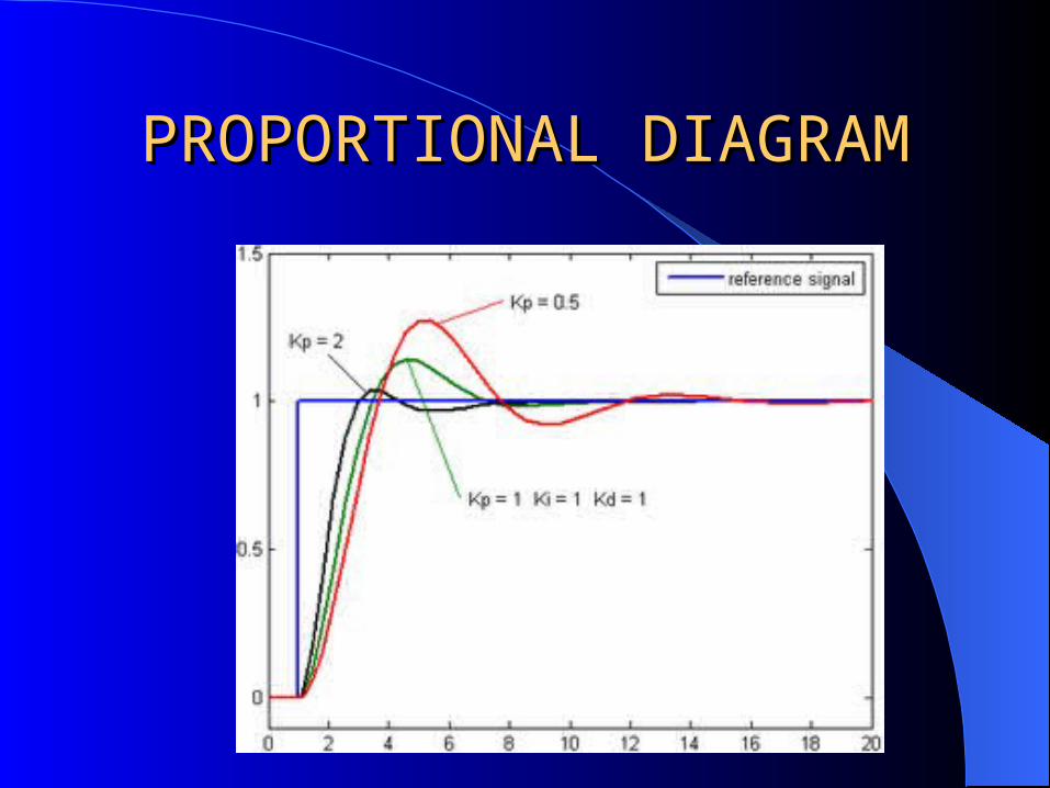
PROPORTIONAL DIAGRAMPROPORTIONAL DIAGRAM

Integral ResponseIntegral Response

The integral component sums the error term over time. The result is that even a small error term will cause the integral component to increase slowly. The integral response will continually increase over time unless the error is zero, so the effect is to drive the Steady-State error to zero. Steady-State error is the final difference between the process variable and set point. A phenomenon called integral windup results when integral action saturates a controller without the controller driving the error signal toward zero.

INTEGRAL DIAGRAMINTEGRAL DIAGRAM

Derivative ResponseDerivative Response

The derivative component causes the output to decrease if the process variable is increasing rapidly. The derivative response is proportional to the rate of change of the process variable. Increasing the derivative time (Td) parameter will cause the control system to react more strongly to changes in the error term and will increase the speed of the overall control system response. Most practical control systems use very small derivative time (Td), because the Derivative Response is highly sensitive to noise in the process variable signal. If the sensor feedback signal is noisy or if the control loop rate is too slow, the derivative response can make the control system unstable

DERIVATIVE DIAGRAMDERIVATIVE DIAGRAM

PID ConceptPID ConceptThe PID instruction can be operated in the timed

mode or the Selectable Time Interrupt (STI mode). In the timed mode, the instruction updates its output periodically at a user-selectable rate. In the STI mode, the instruction should be placed in an STI interrupt subroutine. It then updates its output every time the STI subroutine is scanned. The STI time interval and the PID loop update rate must be the same in order for the equation to execute properly.

PID InstructionPID Instruction

PID TuningPID Tuning

PID tuning is a difficult process. However there are some simple algorithms to follow to get a system approximately tuned.

Sample PID ApplicationSample PID Application

PID Tuning TabPID Tuning Tab

PID Configuration TabPID Configuration Tab

PID Scaling TabPID Scaling Tab

Sample ValuesSample Values

Sample ValuesSample Values

Sample ValuesSample Values

Sample ValuesSample Values

1. Enter an initial set of tuning constants from experience. A conservative setting would be a gain of 1 or less and a reset of less than 0.1.2. Put loop in automatic with process "lined out".3. Make step changes (about 5%) in setpoint.4. Compare response with diagrams and adjust.

On-line trial tuningor 

The "by-guess-and-by-golly" method

Ziegler Nichols tuning method: Ziegler Nichols tuning method: closed loopclosed loop

Steps Place controller into automatic with low gain, no

reset or derivative. Gradually increase gain, making small changes in

the setpoint, until oscillations start. Adjust gain to make the oscillations continue with

a constant amplitude. Note the gain (Ultimate Gain, Gu,) and Period

(Ultimate Period, Pu.) The Ultimate Gain, Gu, is the gain at which the

oscillations continue with a constant amplitude

The gain, reset, and Derivative are calculated using:

  Gain Reset Derivative

P 0.5 GU — —

PI 0.45 GU 1.2/Pu —

PID 0.6 GU 2/Pu Pu/8

Manipulate Proportional

and

Integral terms

Attain these Graphs

Manipulate

Derivative term

Ideal Response

Oscillation

Double Integral Response

Slow Response

Scaling Tab

Unscaled / Eng Max PV 4000

Unscaled / Eng Min PV -4000

CV Max at 100% - 100 What would 50% be? ____

CV Max at 0% - 100

Tuning Tab

Proportional 1 10: to 1 relationship between P:I

Integral .1

Derivative 0

 

Configuration Tab100 CV high Limit (PID Max not CV max)-100 CV Low Limit 0.1  Update time balance with integral(reset) value 

PV and CVMust be RealData Type for

Version 15