
Property calculation II - MIT OpenCourseWare · PDF fileProperty calculation II. ... Basic...
86
1 1.021, 3.021, 10.333, 22.00 Introduction to Modeling and Simulation Spring 2011 Part I – Continuum and particle methods Markus J. Buehler Laboratory for Atomistic and Molecular Mechanics Department of Civil and Environmental Engineering Massachusetts Institute of Technology Property calculation II Lecture 4
-
Upload
phungkhuong -
Category
Documents
-
view
228 -
download
5
Transcript of Property calculation II - MIT OpenCourseWare · PDF fileProperty calculation II. ... Basic...
1
1.021, 3.021, 10.333, 22.00 Introduction to Modeling and SimulationSpring 2011
Part I – Continuum and particle methods
Markus J. BuehlerLaboratory for Atomistic and Molecular MechanicsDepartment of Civil and Environmental EngineeringMassachusetts Institute of Technology
Property calculation IILecture 4
2
Content overview
I. Particle and continuum methods1. Atoms, molecules, chemistry2. Continuum modeling approaches and solution approaches 3. Statistical mechanics4. Molecular dynamics, Monte Carlo5. Visualization and data analysis 6. Mechanical properties – application: how things fail (and
how to prevent it)7. Multi-scale modeling paradigm8. Biological systems (simulation in biophysics) – how
proteins work and how to model them
II. Quantum mechanical methods1. It’s A Quantum World: The Theory of Quantum Mechanics2. Quantum Mechanics: Practice Makes Perfect3. The Many-Body Problem: From Many-Body to Single-
Particle4. Quantum modeling of materials5. From Atoms to Solids6. Basic properties of materials7. Advanced properties of materials8. What else can we do?
Lectures 2-13
Lectures 14-26
3
Overview: Material covered so far…
Lecture 1: Broad introduction to IM/S
Lecture 2: Introduction to atomistic and continuummodeling (multi-scale modeling paradigm, difference between continuum and atomistic approach, case study: diffusion)
Lecture 3: Basic statistical mechanics – property calculation I (property calculation: microscopic states vs. macroscopic properties, ensembles, probability density and partition function)
Lecture 4: Property calculation II (Advanced property calculation, introduction to chemical interactions, Monte Carlo methods)
4
Lecture 4: Property calculation II
Outline:
1. Advanced analysis methods: Radial distribution function (RDF)2. Introduction: How to model chemical interactions
2.1 How to identify parameters in a Lennard-Jones potential3. Monte-Carlo (MC) approach: Metropolis-Hastings algorithm
3.1 Application to integration 3.2 Metropolis-Hastings algorithm
Goal of today’s lecture:
- Learn how to analyze structure of a material based on atomistic simulation result (solid, liquid, gas, different crystal structure, etc.)
- Introduction to potential or force field (Lennard-Jones) - Present details of MC algorithm – background and
implementation
5
1. Advanced analysis methods: Radial distribution function (RDF)
6
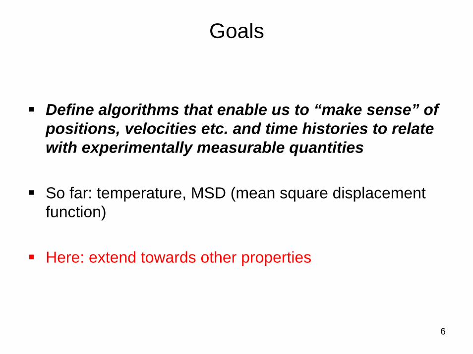
Goals
Define algorithms that enable us to “make sense” of positions, velocities etc. and time histories to relate with experimentally measurable quantities
So far: temperature, MSD (mean square displacement function)
Here: extend towards other properties

7
MD modeling of crystals – solid, liquid, gas phase
Crystals: Regular, ordered structure
The corresponding particle motions are small-amplitude vibrations about the lattice site, diffusive movements over a local region, and long free flights interrupted by a collision every now and then.
Liquids: Particles follow Brownian motion (collisions)
Gas: Very long free paths
Image by MIT OpenCourseWare. After J. A. Barker and D. Henderson.
8
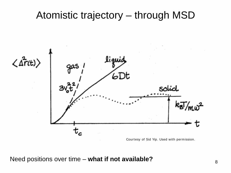
Atomistic trajectory – through MSD
Need positions over time – what if not available?
Courtesy of Sid Yip. Used with permission.
9
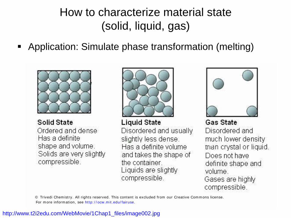
How to characterize material state (solid, liquid, gas)
Application: Simulate phase transformation (melting)
http://www.t2i2edu.com/WebMovie/1Chap1_files/image002.jpg
© Trivedi Chemistry. All rights reserved. This content is excluded from our Creative Commons license.For more information, see http://ocw.mit.edu/fairuse.
10
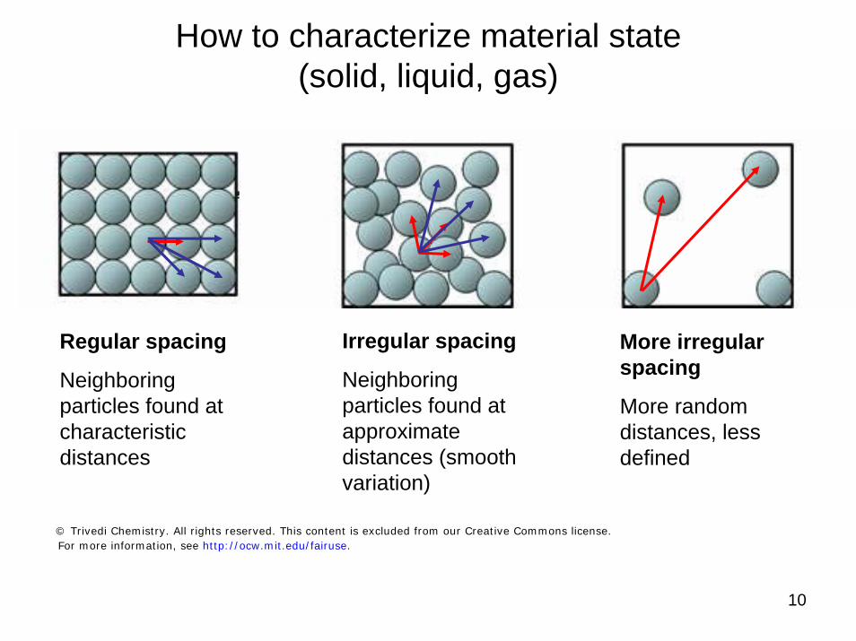
How to characterize material state (solid, liquid, gas)
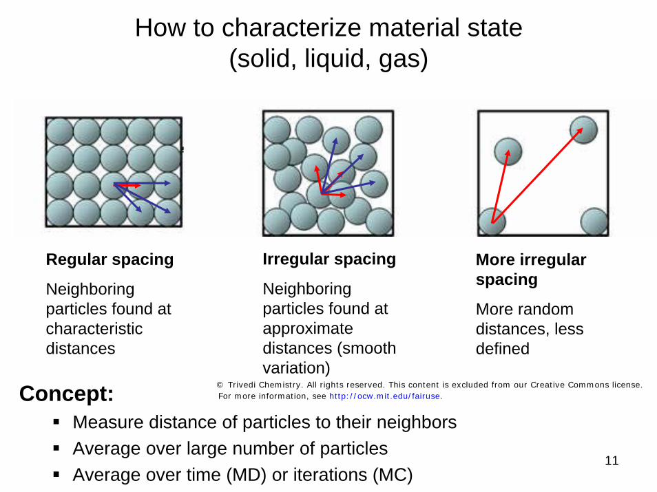
Regular spacing
Neighboring particles found at characteristic distances
Irregular spacing
Neighboring particles found at approximate distances (smooth variation)
More irregular spacing
More random distances, less defined
© Trivedi Chemistry. All rights reserved. This content is excluded from our Creative Commons license.For more information, see http://ocw.mit.edu/fairuse.
11
How to characterize material state (solid, liquid, gas)
Concept:Measure distance of particles to their neighborsAverage over large number of particlesAverage over time (MD) or iterations (MC)
Regular spacing
Neighboring particles found at characteristic distances
Irregular spacing
Neighboring particles found at approximate distances (smooth variation)
More irregular spacing
More random distances, less defined
© Trivedi Chemistry. All rights reserved. This content is excluded from our Creative Commons license.For more information, see http://ocw.mit.edu/fairuse.
12
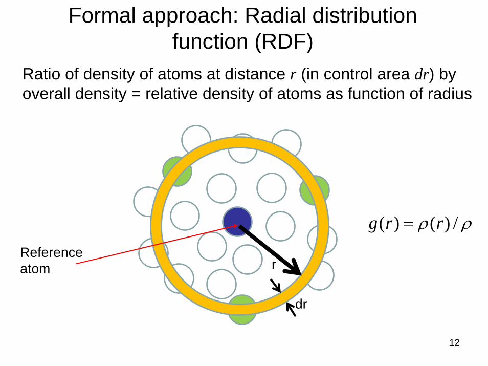
Reference atom
Formal approach: Radial distribution function (RDF)
ρρ /)()( rrg =
Ratio of density of atoms at distance r (in control area dr) by overall density = relative density of atoms as function of radius
r
dr

13
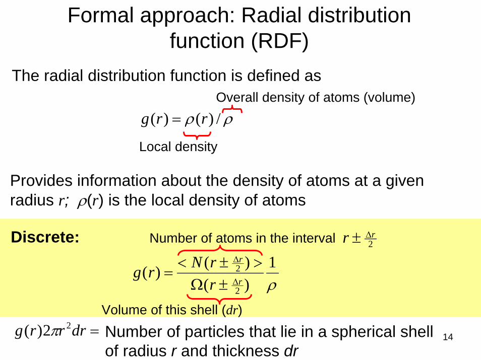
Formal approach: Radial distribution function (RDF)
ρρ /)()( rrg =
The radial distribution function is defined as
Local density
Overall density of atoms (volume)
Provides information about the density of atoms at a given radius r; ρ(r) is the local density of atoms
14
Formal approach: Radial distribution function (RDF)
ρρ /)()( rrg =
The radial distribution function is defined as
Provides information about the density of atoms at a given radius r; ρ(r) is the local density of atoms
ρ1
)()()(
2
2r
r
rrNrg
Δ
Δ
±Ω>±<
=
=drrrg 22)( π Number of particles that lie in a spherical shellof radius r and thickness dr
Local density
Overall density of atoms (volume)
Volume of this shell (dr)
Number of atoms in the interval 2rr Δ±Discrete:
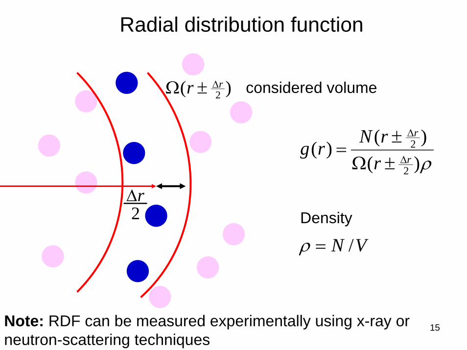
15
Radial distribution function
ρ)()()(
2
2r
r
rrNrg
Δ
Δ
±Ω±
=
VN /=ρDensity
Note: RDF can be measured experimentally using x-ray or neutron-scattering techniques
)( 2rr Δ±Ω considered volume
2rΔ

16
Radial distribution function: Which one is solid / liquid?
Interpretation: A peak indicates a particularlyfavored separation distance for the neighbors to a given particleThus, RDF reveals details about the atomic structure of the system being simulatedJava applet:http://physchem.ox.ac.uk/~rkt/lectures/liqsolns/liquids.html
© source unknown. All rights reserved. This content is excluded from our Creative Commons license. For more information, see http://ocw.mit.edu/fairuse.
17
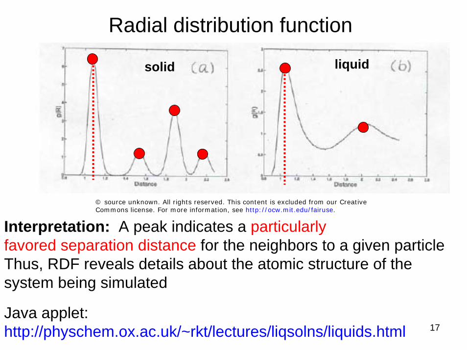
Radial distribution function
solid liquid
Interpretation: A peak indicates a particularlyfavored separation distance for the neighbors to a given particleThus, RDF reveals details about the atomic structure of the system being simulated
Java applet:http://physchem.ox.ac.uk/~rkt/lectures/liqsolns/liquids.html
© source unknown. All rights reserved. This content is excluded from our Creative Commons license. For more information, see http://ocw.mit.edu/fairuse.
18
Radial distribution function: JAVA applet
Java applet:http://physchem.ox.ac.uk/~rkt/lectures/liqsolns/liquids.html
Image removed for copyright reasons.Screenshot of the radial distribution function Java applet.
19
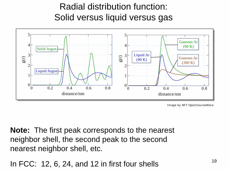
Radial distribution function: Solid versus liquid versus gas
Note: The first peak corresponds to the nearest neighbor shell, the second peak to the second nearest neighbor shell, etc.
In FCC: 12, 6, 24, and 12 in first four shells
Image by MIT OpenCourseWare.
5
4
3
2
1
00 0.2 0.4 0.6 0.8
g(r)
distance/nm
5
4
3
2
1
00 0.2 0.4 0.6 0.8
g(r)
distance/nm
Solid Argon
Liquid Argon
Liquid Ar(90 K)
Gaseous Ar(90 K)
Gaseous Ar(300 K)
20
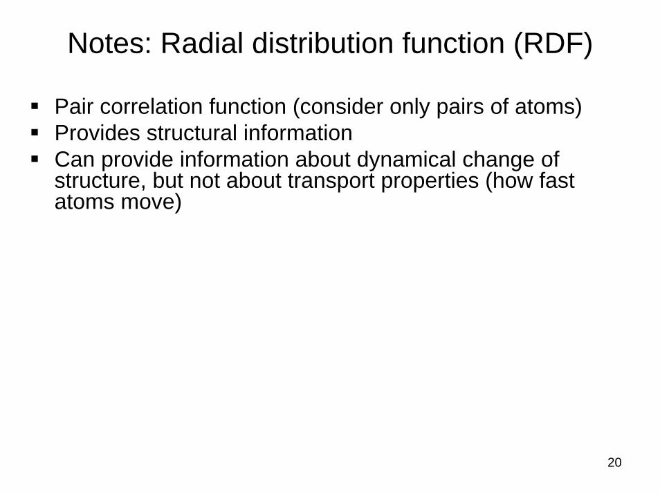
Notes: Radial distribution function (RDF)
Pair correlation function (consider only pairs of atoms)Provides structural informationCan provide information about dynamical change of structure, but not about transport properties (how fast atoms move)
21
Notes: Radial distribution function (RDF)
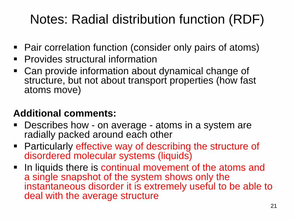
Pair correlation function (consider only pairs of atoms)Provides structural informationCan provide information about dynamical change of structure, but not about transport properties (how fast atoms move)
Additional comments:Describes how - on average - atoms in a system are radially packed around each other Particularly effective way of describing the structure of disordered molecular systems (liquids)In liquids there is continual movement of the atoms and a single snapshot of the system shows only the instantaneous disorder it is extremely useful to be able to deal with the average structure
22
Example RDFs for several materials
2nd NN
3rd NN
…
23
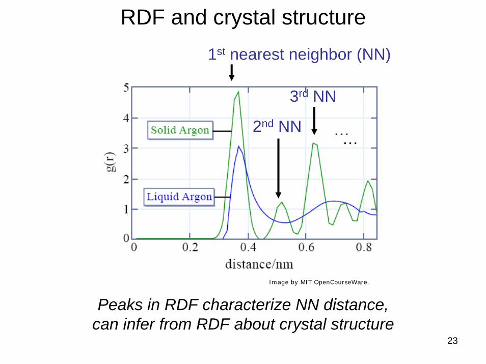
RDF and crystal structure1st nearest neighbor (NN)
Peaks in RDF characterize NN distance, can infer from RDF about crystal structure
Image by MIT OpenCourseWare.
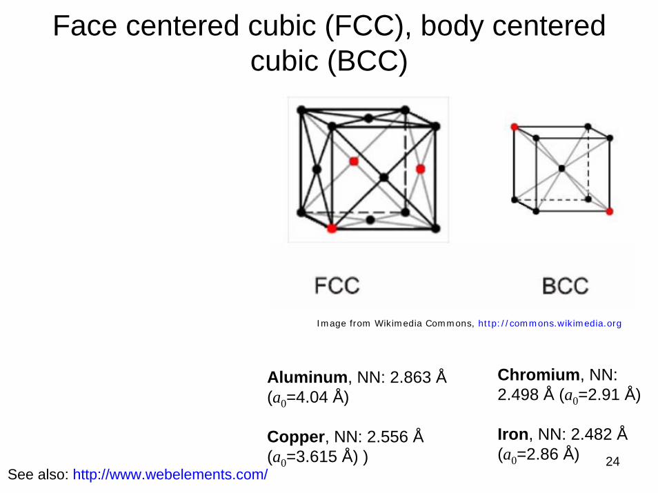
Face centered cubic (FCC), body centered cubic (BCC)
Aluminum, NN: 2.863 Å(a0=4.04 Å)
Copper, NN: 2.556 Å(a0=3.615 Å) )
Chromium, NN: 2.498 Å (a0=2.91 Å)
Iron, NN: 2.482 Å(a0=2.86 Å)
See also: http://www.webelements.com/24
Image from Wikimedia Commons, http://commons.wikimedia.org
25
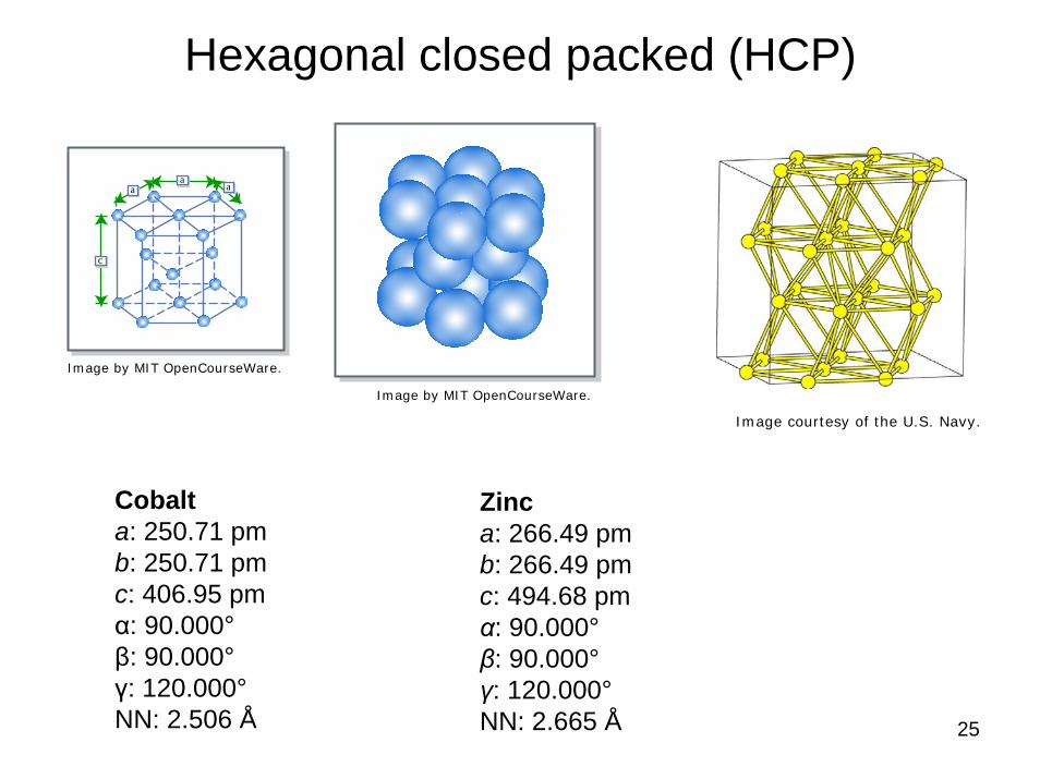
Hexagonal closed packed (HCP)
Cobalta: 250.71 pm b: 250.71 pm c: 406.95 pm α: 90.000°β: 90.000°γ: 120.000°NN: 2.506 Å
Zinca: 266.49 pm b: 266.49 pm c: 494.68 pm α: 90.000°β: 90.000°γ: 120.000°NN: 2.665 Å
Image courtesy of the U.S. Navy.
Image by MIT OpenCourseWare.
aa
a
c
Image by MIT OpenCourseWare.
26
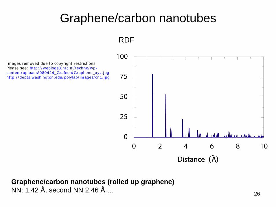
Graphene/carbon nanotubes
Graphene/carbon nanotubes (rolled up graphene)NN: 1.42 Å, second NN 2.46 Å …
RDF
Images removed due to copyright restrictions.Please see: http://weblogs3.nrc.nl/techno/wp-content/uploads/080424_Grafeen/Graphene_xyz.jpghttp://depts.washington.edu/polylab/images/cn1.jpg
27
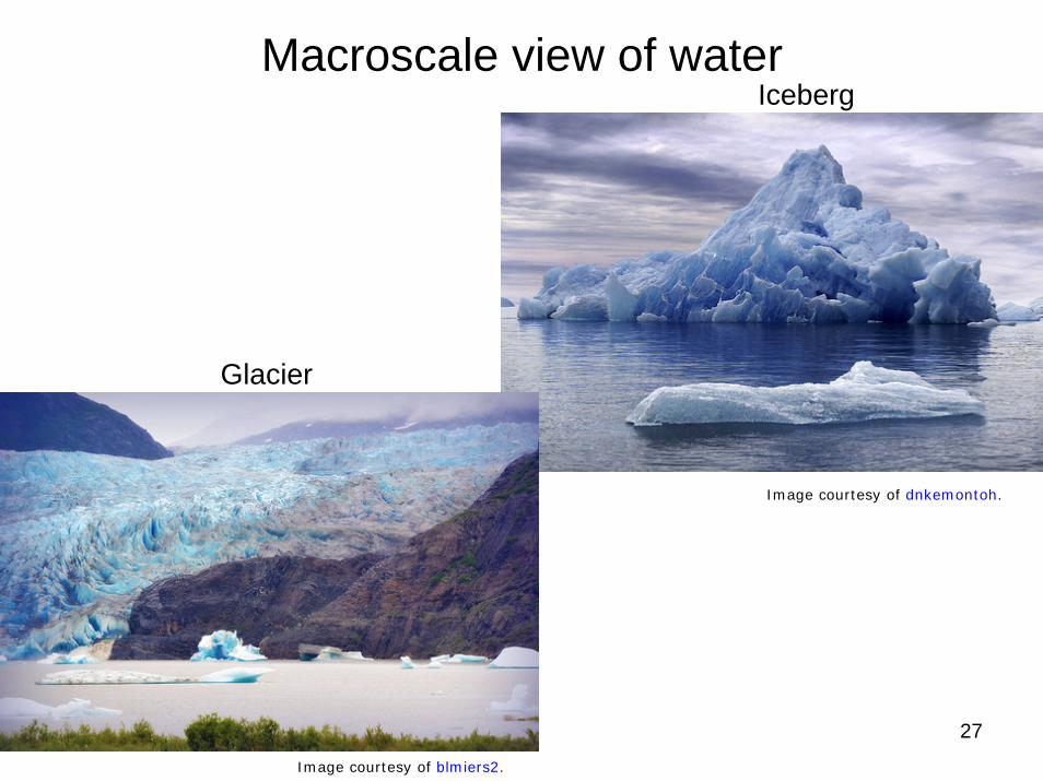
Macroscale view of waterIceberg
Glacier
Image courtesy of dnkemontoh.
Image courtesy of blmiers2.
28
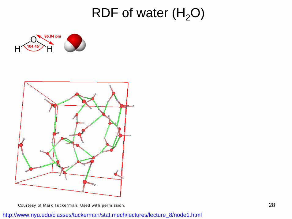
RDF of water (H2O)
http://www.nyu.edu/classes/tuckerman/stat.mech/lectures/lecture_8/node1.html
Courtesy of Mark Tuckerman. Used with permission.
29
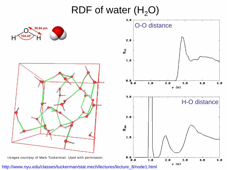
RDF of water (H2O)O-O distance
H-O distance
http://www.nyu.edu/classes/tuckerman/stat.mech/lectures/lecture_8/node1.html
Images courtesy of Mark Tuckerman. Used with permission.
30
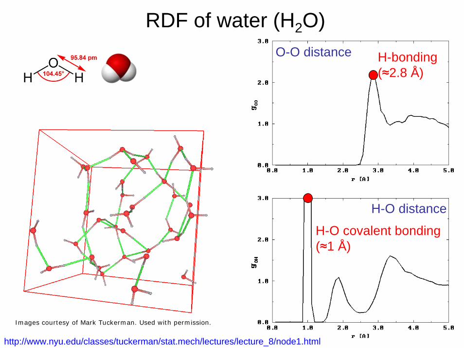
RDF of water (H2O)O-O distance
H-O distance
H-bonding(≈2.8 Å)
H-O covalent bonding(≈1 Å)
http://www.nyu.edu/classes/tuckerman/stat.mech/lectures/lecture_8/node1.html
Images courtesy of Mark Tuckerman. Used with permission.
31
2. Introduction: How to model chemical interactions
32
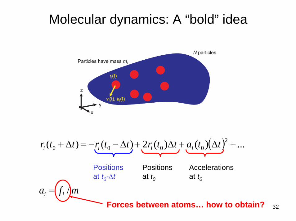
Molecular dynamics: A “bold” idea
( ) ...)()(2)()( 20000 +Δ+Δ+Δ−−=Δ+ ttattrttrttr iiii
Positions at t0
Accelerationsat t0
Positions at t0-Δt
mfa ii /=Forces between atoms… how to obtain?
33
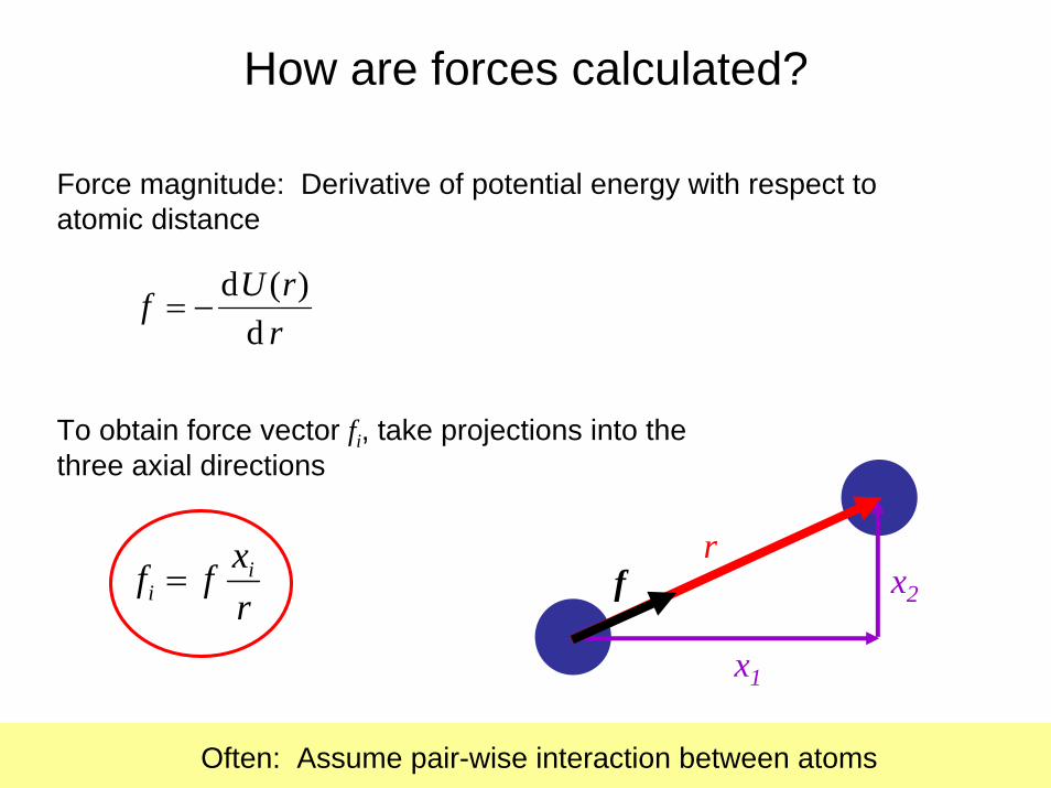
rrUf
d)(d
−=
Force magnitude: Derivative of potential energy with respect toatomic distance
To obtain force vector fi, take projections into the three axial directions
rxff i
i =r
x1
x2f
Often: Assume pair-wise interaction between atoms
How are forces calculated?
34
Atomic interactions – quantum perspective
Much more about it in part II
How electrons from different atoms interact defines nature of chemical bond
Density distribution of electrons around a H-H molecule
Image removed due to copyright restrictions. Please see the animation of hydrogen bonding orbitals at http://winter.group.shef.ac.uk/orbitron/MOs/H2/1s1s-sigma/index.html

35
Concept: Interatomic potential
“point particle” representation
Attraction: Formation of chemical bond by sharing of electronsRepulsion: Pauli exclusion (too many electrons in small volume)
Image by MIT OpenCourseWare.
e
Energy U r
Repulsion
Attraction
1/r12 (or Exponential)
1/r6
Radius r (Distance between atoms)
36
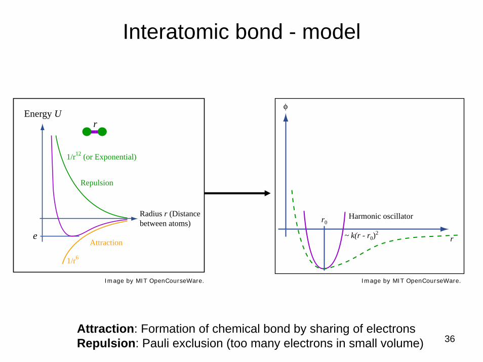
Interatomic bond - model
Attraction: Formation of chemical bond by sharing of electronsRepulsion: Pauli exclusion (too many electrons in small volume)
Image by MIT OpenCourseWare. Image by MIT OpenCourseWare.
Harmonic oscillatorr0
φ
r~ k(r - r0)2e
Energy U r
Repulsion
Attraction
1/r12 (or Exponential)
1/r6
Radius r (Distance between atoms)
37
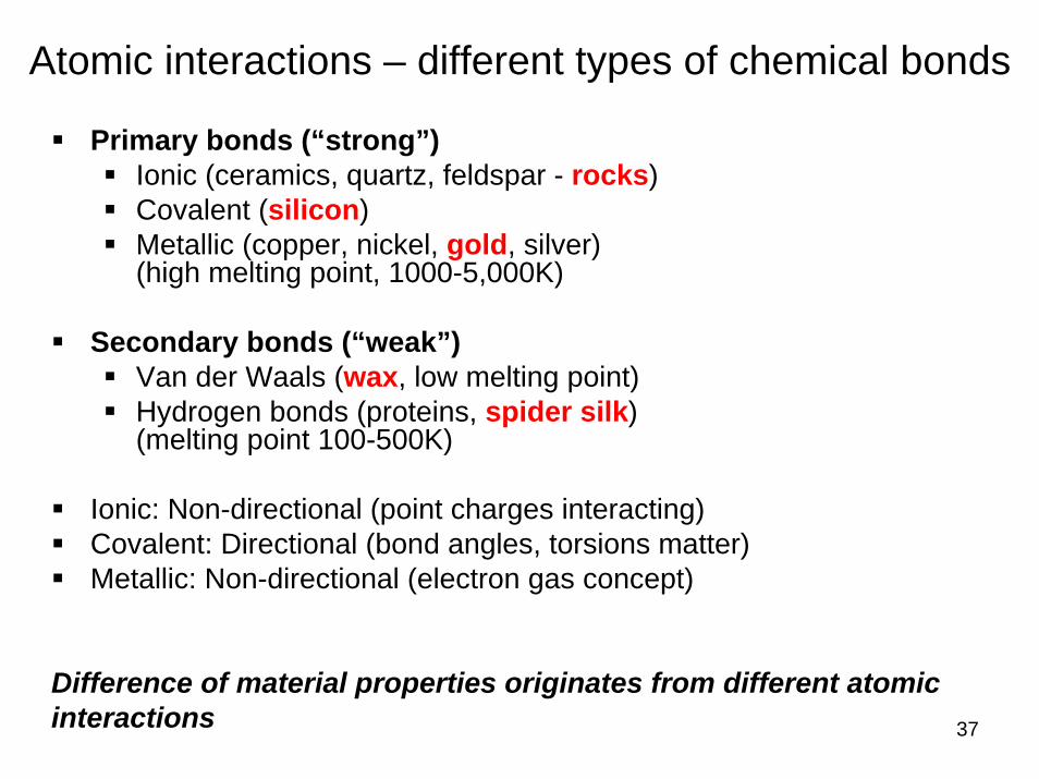
Atomic interactions – different types of chemical bonds
Primary bonds (“strong”)Ionic (ceramics, quartz, feldspar - rocks) Covalent (silicon) Metallic (copper, nickel, gold, silver)(high melting point, 1000-5,000K)
Secondary bonds (“weak”)Van der Waals (wax, low melting point) Hydrogen bonds (proteins, spider silk)(melting point 100-500K)
Ionic: Non-directional (point charges interacting)Covalent: Directional (bond angles, torsions matter)Metallic: Non-directional (electron gas concept)
Difference of material properties originates from different atomic interactions
38
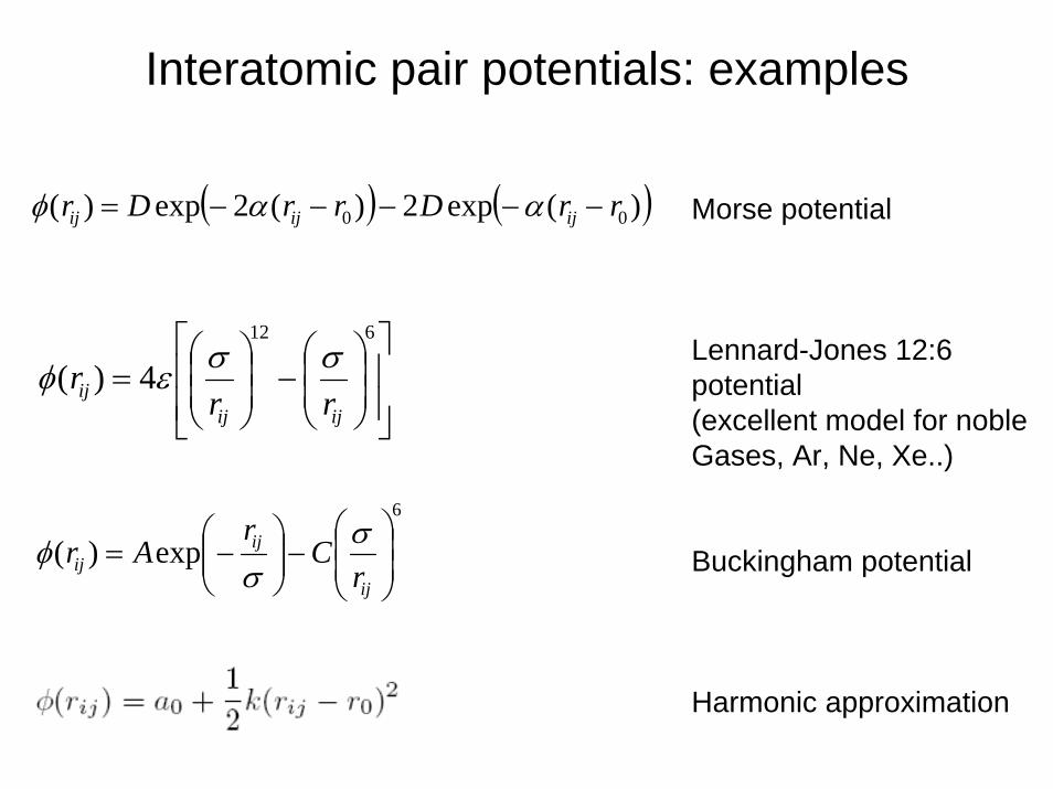
Interatomic pair potentials: examples
Morse potential
Lennard-Jones 12:6 potential(excellent model for nobleGases, Ar, Ne, Xe..)
Buckingham potential
Harmonic approximation
( ) ( ))(exp2)(2exp)( 00 rrDrrDr ijijij −−−−−= ααφ
6
exp)( ⎟⎟⎠
⎞⎜⎜⎝
⎛−⎟⎟
⎠
⎞⎜⎜⎝
⎛−=
ij
ijij r
Cr
Ar σσ
φ
⎥⎥
⎦
⎤
⎢⎢
⎣
⎡
⎟⎟⎠
⎞⎜⎜⎝
⎛−⎟
⎟⎠
⎞⎜⎜⎝
⎛=
612
4)(ijij
ij rrr σσεφ
39
What is the difference between these models?
Shape of potential (e.g. behavior at short or long distances, around equilibrium)
Number of parameters (to fit)Ability to describe bond breaking
40
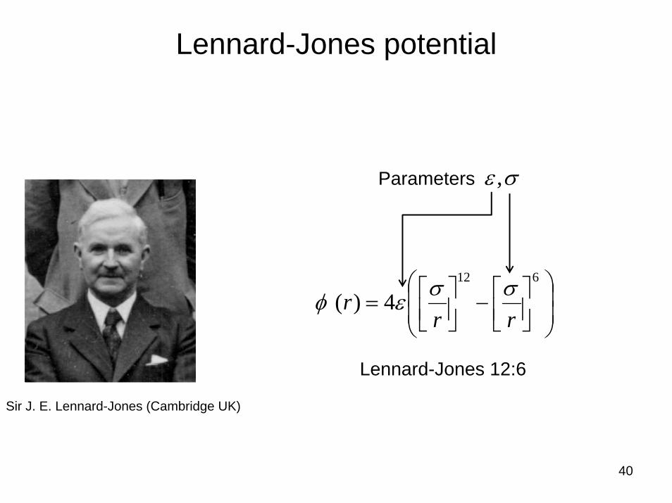
Lennard-Jones potential
Lennard-Jones 12:6
Parameters
⎟⎟⎠
⎞⎜⎜⎝
⎛⎥⎦⎤
⎢⎣⎡−⎥⎦
⎤⎢⎣⎡=
612
4)(rr
r σσεφ
σε ,
Sir J. E. Lennard-Jones (Cambridge UK)
41
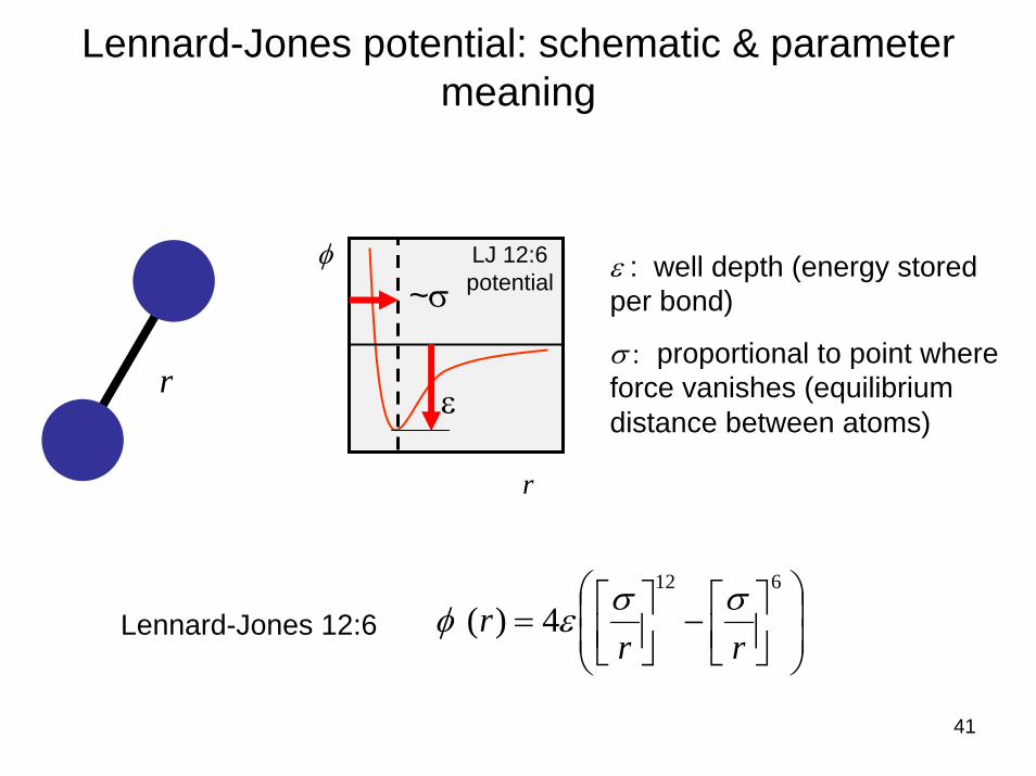
Lennard-Jones potential: schematic & parameter meaning
φ
r
LJ 12:6potential
Lennard-Jones 12:6
r ε
~σ
⎟⎟⎠
⎞⎜⎜⎝
⎛⎥⎦⎤
⎢⎣⎡−⎥⎦
⎤⎢⎣⎡=
612
4)(rr
r σσεφ
ε : well depth (energy stored per bond)
σ : proportional to point where force vanishes (equilibrium distance between atoms)
42
2.1 How to identify parameters in a Lennard-Jones potential
(=force field training, force field fitting, parameter coupling, etc.)
43
Parameter identification for potentials
Typically done based on more accurate (e.g. quantum mechanical) results (or experimental measurements, if available)
Properties used include:
Lattice constant, cohesive bond energy, elastic modulus (bulk, shear, …), equations of state, phonon frequencies (bond vibrations), forces, stability/energy of different crystal structures, surface energy, RDF, etc.
Potential should closely reproduce these reference values
Challenges: mixed systems, different types of bonds, reactions
44
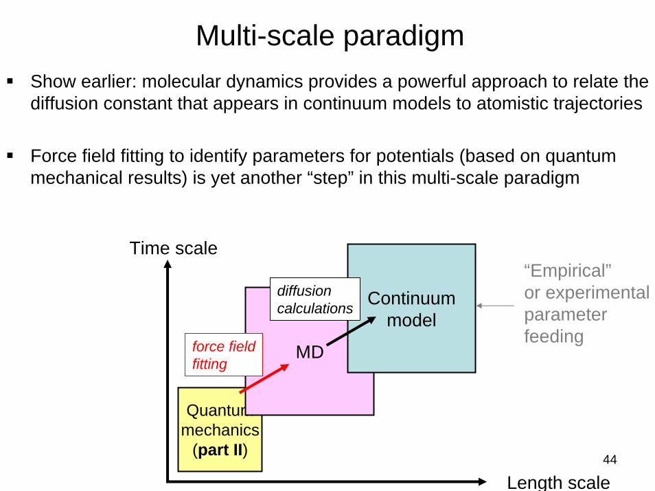
Quantummechanics
(part II)
Multi-scale paradigmShow earlier: molecular dynamics provides a powerful approach to relate the diffusion constant that appears in continuum models to atomistic trajectories
Force field fitting to identify parameters for potentials (based on quantum mechanical results) is yet another “step” in this multi-scale paradigm
MD
Continuummodel
Length scale
Time scale“Empirical”or experimentalparameterfeedingforce field
fitting
diffusioncalculations
45
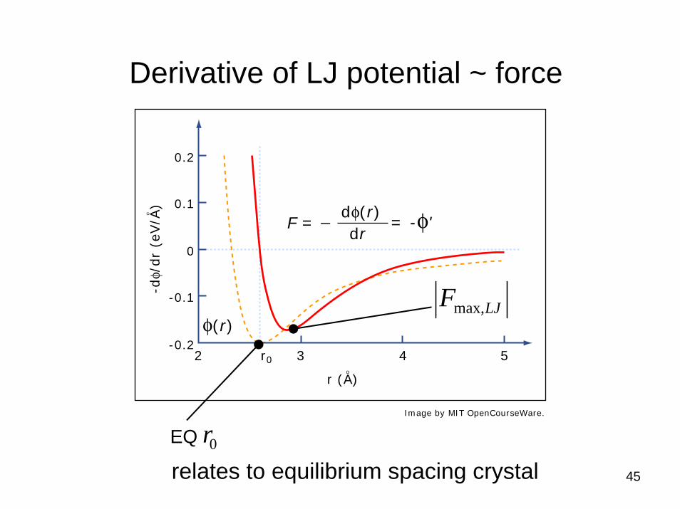
Derivative of LJ potential ~ force
relates to equilibrium spacing crystal
0.2
0.1
0
-0.1
-0.22 3 4 5r0
-dφ/
dr
(eV/A
)ο
r (A)o
F = _ dφ(r)dr
= -φ'
LJFmax,
rEQ
φ(r)
0
Image by MIT OpenCourseWare.
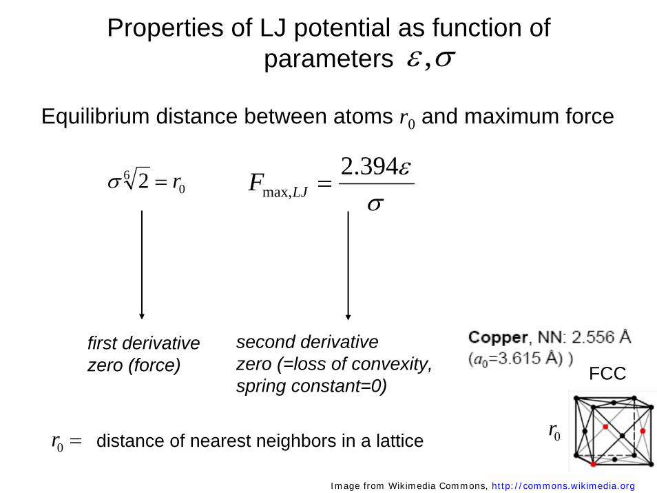
Properties of LJ potential as function of parameters
Equilibrium distance between atoms r0 and maximum force
06 2 r=σ
σε394.2
max, =LJF
first derivative zero (force)
second derivative zero (=loss of convexity, spring constant=0)
=0r distance of nearest neighbors in a lattice 0r
FCC
σε ,
Image from Wikimedia Commons, http://commons.wikimedia.org
47
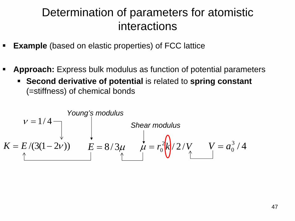
Determination of parameters for atomistic interactions
Example (based on elastic properties) of FCC lattice
Approach: Express bulk modulus as function of potential parametersSecond derivative of potential is related to spring constant(=stiffness) of chemical bonds
Shear modulusYoung’s modulus
μ3/8=E))21(3/( ν−= EK
4/1=ν
Vkr /2/20=μ 4/3
0aV =
48
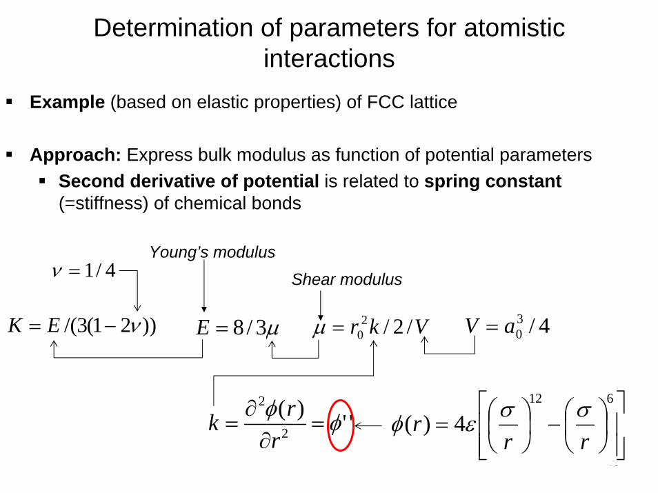
Determination of parameters for atomistic interactions
Example (based on elastic properties) of FCC lattice
Approach: Express bulk modulus as function of potential parametersSecond derivative of potential is related to spring constant(=stiffness) of chemical bonds
'')(2
2
φφ=
∂∂
=r
rk⎥⎥⎦
⎤
⎢⎢⎣
⎡⎟⎠⎞
⎜⎝⎛−⎟
⎠⎞
⎜⎝⎛=
612
4)(rr
r σσεφ
Shear modulusYoung’s modulus
μ3/8=E))21(3/( ν−= EK Vkr /2/20=μ 4/3
0aV =
4/1=ν
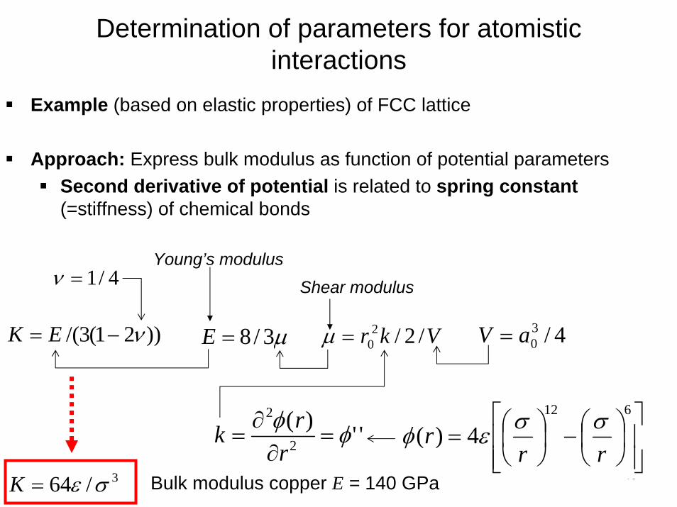
493/64 σε=K
Determination of parameters for atomistic interactions
Example (based on elastic properties) of FCC lattice
Approach: Express bulk modulus as function of potential parametersSecond derivative of potential is related to spring constant(=stiffness) of chemical bonds
⎥⎥⎦
⎤
⎢⎢⎣
⎡⎟⎠⎞
⎜⎝⎛−⎟
⎠⎞
⎜⎝⎛=
612
4)(rr
r σσεφ
Shear modulusYoung’s modulus
μ3/8=E))21(3/( ν−= EK Vkr /2/20=μ 4/3
0aV =
4/1=ν
'')(2
2
φφ=
∂∂
=r
rk
Bulk modulus copper E = 140 GPa
50
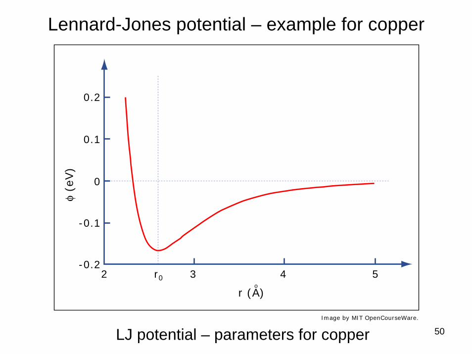
Lennard-Jones potential – example for copper
LJ potential – parameters for copperImage by MIT OpenCourseWare.
0.2
0.1
0
2 3 4 5
-0.1
-0.2r0
φ (e
V)
r (A)o

51
3. Monte Carlo approaches
52
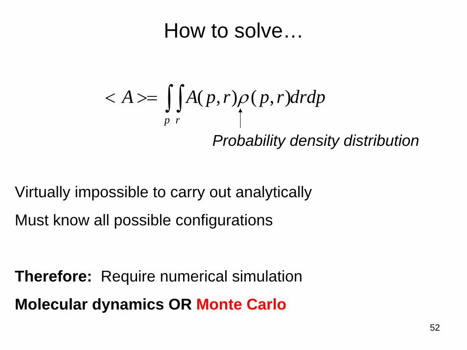
How to solve…
drdprprpAAp r∫ ∫>=< ),(),( ρ
Probability density distribution
Virtually impossible to carry out analytically
Must know all possible configurations
Therefore: Require numerical simulation
Molecular dynamics OR Monte Carlo
53
3.1 Application to integration
“Random sampling”
54
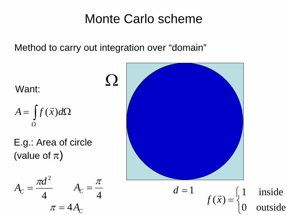
Monte Carlo scheme
∫Ω
Ω= dxfA )(
Method to carry out integration over “domain”
Want:
E.g.: Area of circle (value of π)
4
2dACπ
=4π
=CA 1=d
Ω
⎩⎨⎧
=outside0inside1
)(xfCA4=π
55
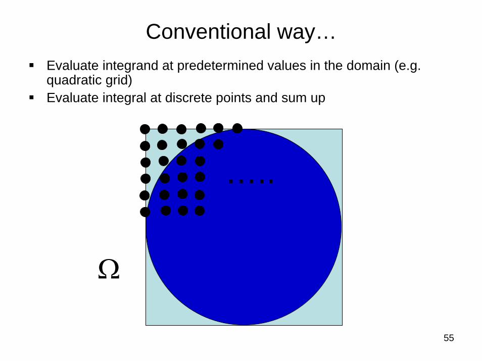
Conventional way…Evaluate integrand at predetermined values in the domain (e.g. quadratic grid)Evaluate integral at discrete points and sum up
Ω
…..
56
What about playing darts..
Public domain image.
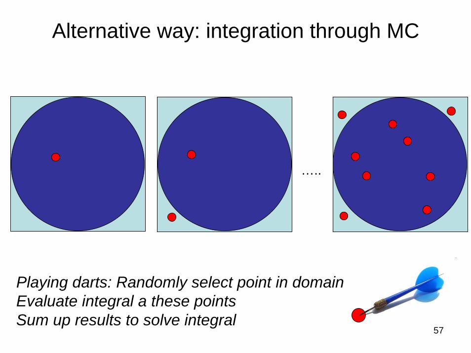
Alternative way: integration through MC
…..
Playing darts: Randomly select point in domainEvaluate integral a these pointsSum up results to solve integral
57
58
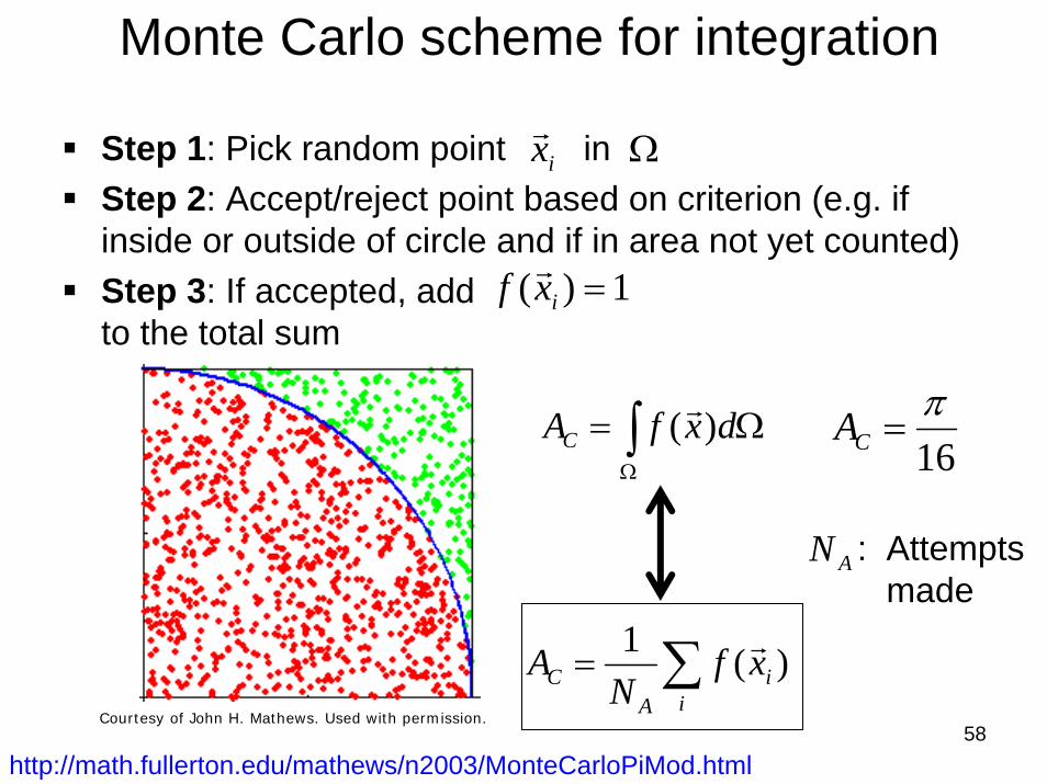
Monte Carlo scheme for integration
Step 1: Pick random point in Step 2: Accept/reject point based on criterion (e.g. if inside or outside of circle and if in area not yet counted)Step 3: If accepted, add to the total sum
Ω
1)( =ixf
ix
∫Ω
Ω= dxfAC )(
∑=i
iA
C xfN
A )(1
http://math.fullerton.edu/mathews/n2003/MonteCarloPiMod.html
AN : Attemptsmade
16π
=CA
Courtesy of John H. Mathews. Used with permission.
59
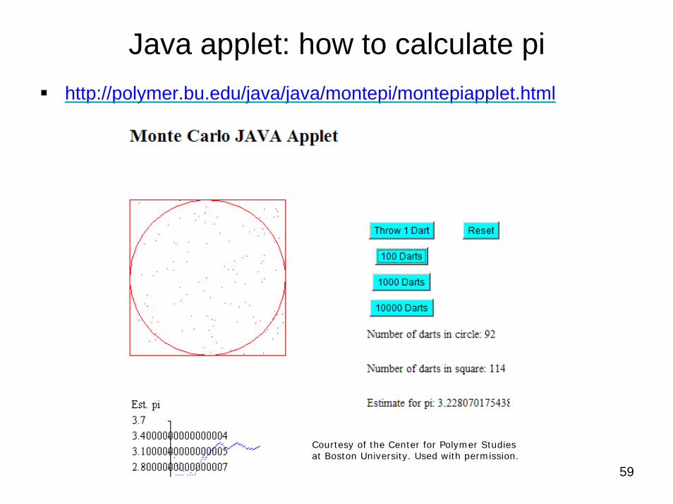
Java applet: how to calculate pihttp://polymer.bu.edu/java/java/montepi/montepiapplet.html
Courtesy of the Center for Polymer Studies at Boston University. Used with permission.
60
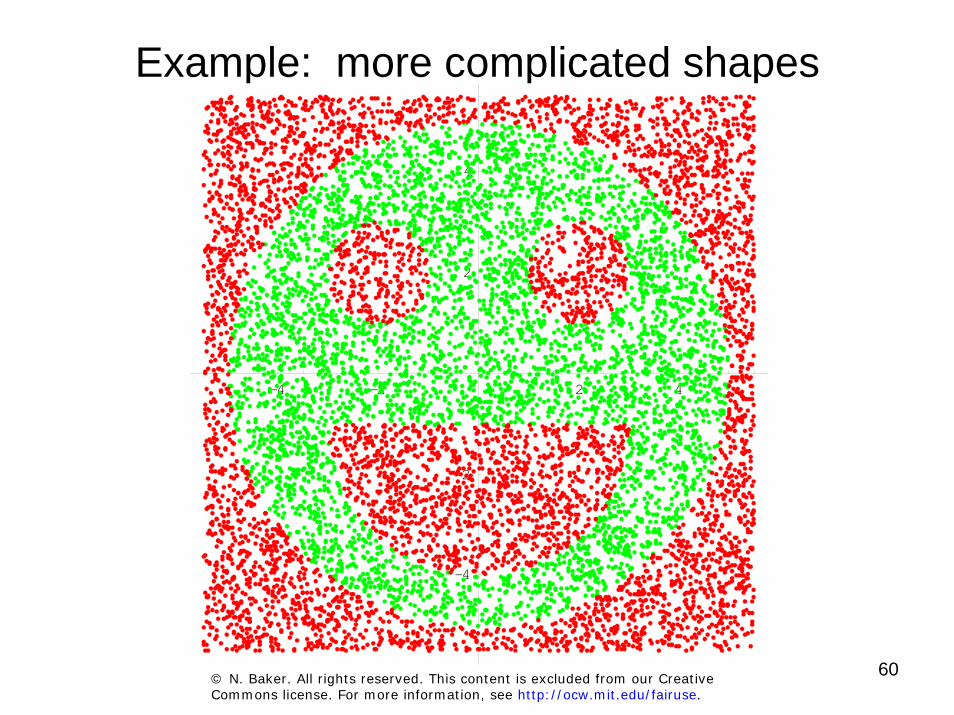
Example: more complicated shapes
-4 -2 2 4
-4
-2
2
4
© N. Baker. All rights reserved. This content is excluded from our Creative Commons license. For more information, see http://ocw.mit.edu/fairuse.
61
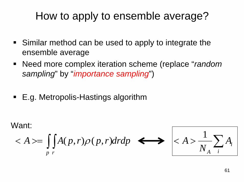
How to apply to ensemble average?
Similar method can be used to apply to integrate the ensemble averageNeed more complex iteration scheme (replace “random sampling” by “importance sampling”)
E.g. Metropolis-Hastings algorithm
drdprprpAAp r∫ ∫>=< ),(),( ρ ∑><
ii
A
AN
A 1Want:
62
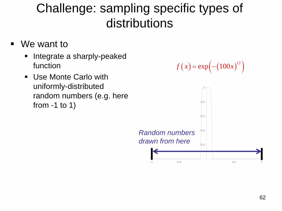
Challenge: sampling specific types of distributions
We want toIntegrate a sharply-peaked functionUse Monte Carlo with uniformly-distributed random numbers (e.g. here from -1 to 1)
-1 -0.5 0.5 1
0.2
0.4
0.6
0.8
1
( ) ( )( )12exp 100f x x= −
Random numbersdrawn from here
63
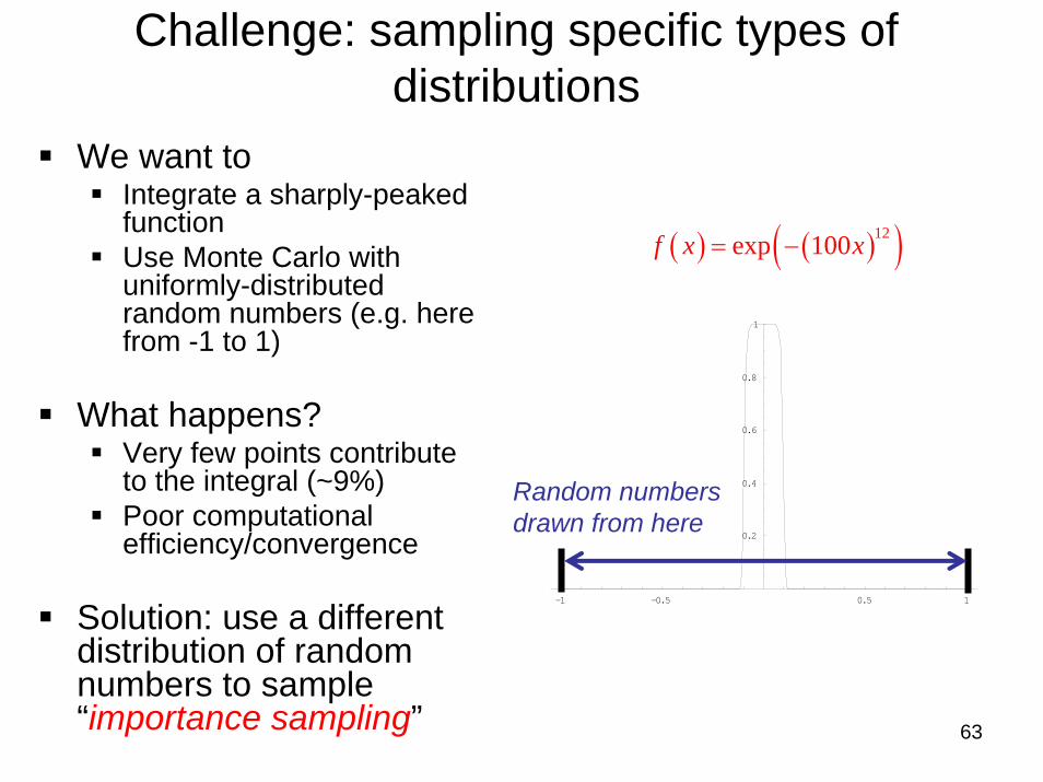
Challenge: sampling specific types of distributions
We want toIntegrate a sharply-peaked functionUse Monte Carlo with uniformly-distributed random numbers (e.g. here from -1 to 1)
What happens?Very few points contribute to the integral (~9%)Poor computational efficiency/convergence
Solution: use a different distribution of random numbers to sample “importance sampling”
-1 -0.5 0.5 1
0.2
0.4
0.6
0.8
1
( ) ( )( )12exp 100f x x= −
Random numbersdrawn from here
64
3.2 Metropolis-Hastings algorithm
“Importance sampling”
65
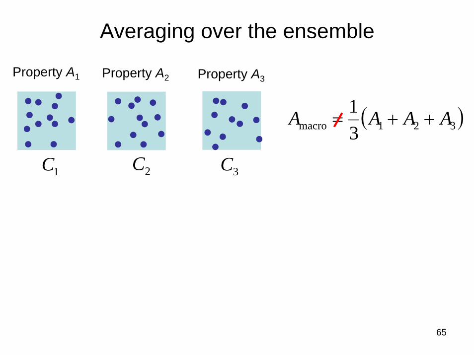
Averaging over the ensemble
1C 2C 3C
Property A1 Property A2 Property A3
( )321macro 31 AAAA ++=
66
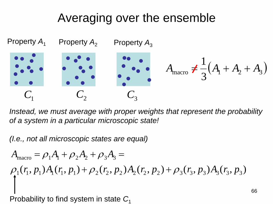
Averaging over the ensemble
1C 2C 3C
Property A1 Property A2 Property A3
( )321macro 31 AAAA ++=
Instead, we must average with proper weights that represent the probability of a system in a particular microscopic state!
(I.e., not all microscopic states are equal)
),(),(),(),(),(),( 333333222222111111
332211macro
prAprprAprprAprAAAA
ρρρρρρ
++=++=
Probability to find system in state C1
67
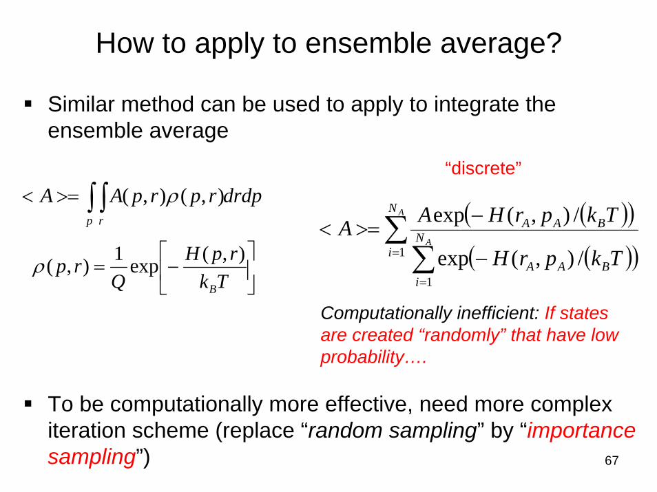
Similar method can be used to apply to integrate the ensemble average
To be computationally more effective, need more complex iteration scheme (replace “random sampling” by “importance sampling”)
How to apply to ensemble average?
⎥⎦
⎤⎢⎣
⎡−=
TkrpH
Qrp
B
),(exp1),(ρ
drdprprpAAp r∫ ∫>=< ),(),( ρ
( )( )
( )( )∑
∑=
=
−
−>=<
A
A
N
iN
iBAA
BAA
TkprH
TkprHAA1
1
/),(exp
/),(exp
“discrete”
Computationally inefficient: If states are created “randomly” that have low probability….
68
Importance sampling
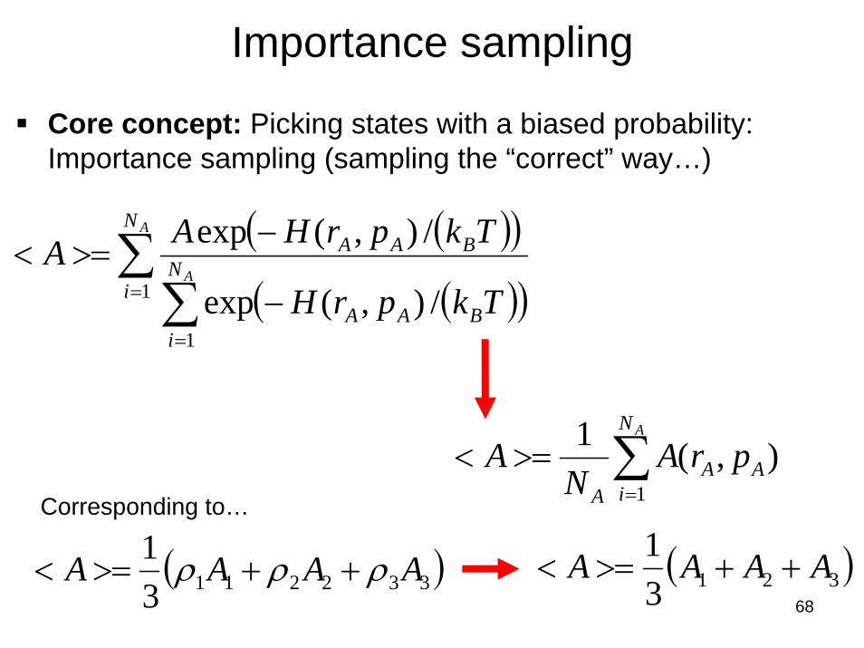
Core concept: Picking states with a biased probability: Importance sampling (sampling the “correct” way…)
( )32131 AAAA ++>=<
( )( )
( )( )∑
∑=
=
−
−>=<
A
A
N
iN
iBAA
BAA
TkprH
TkprHAA1
1/),(exp
/),(exp
( )33221131 AAAA ρρρ ++>=<
∑=
>=<AN
iAA
A
prAN
A1
),(1
Corresponding to…
69
Importance sampling
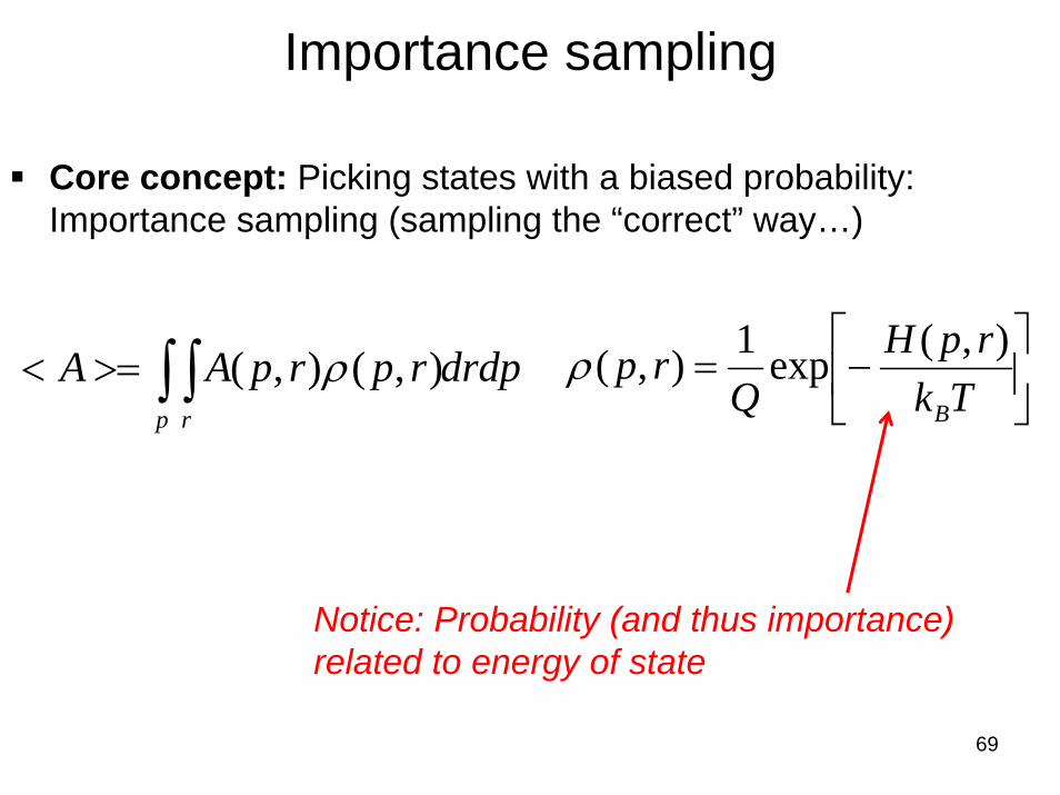
Core concept: Picking states with a biased probability: Importance sampling (sampling the “correct” way…)
⎥⎦
⎤⎢⎣
⎡−=
TkrpH
Qrp
B
),(exp1),(ρdrdprprpAAp r∫ ∫>=< ),(),( ρ
Notice: Probability (and thus importance)related to energy of state
70
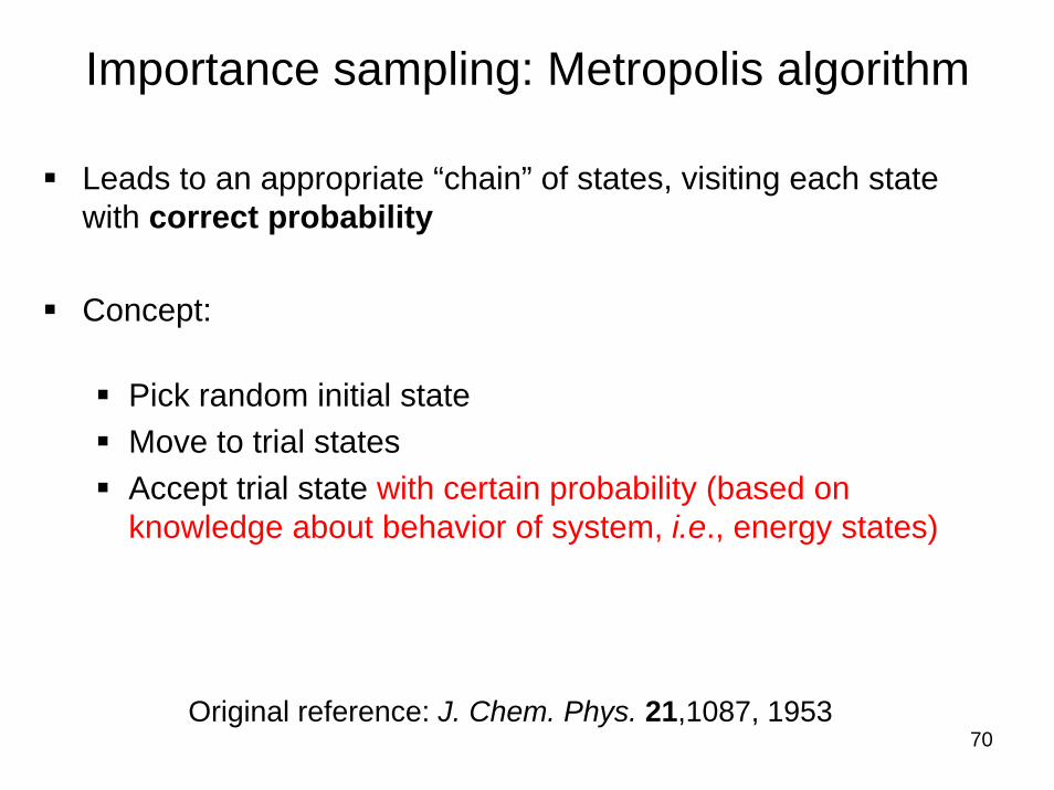
Importance sampling: Metropolis algorithm
Leads to an appropriate “chain” of states, visiting each state with correct probability
Concept:
Pick random initial stateMove to trial statesAccept trial state with certain probability (based on knowledge about behavior of system, i.e., energy states)
Original reference: J. Chem. Phys. 21,1087, 1953
71
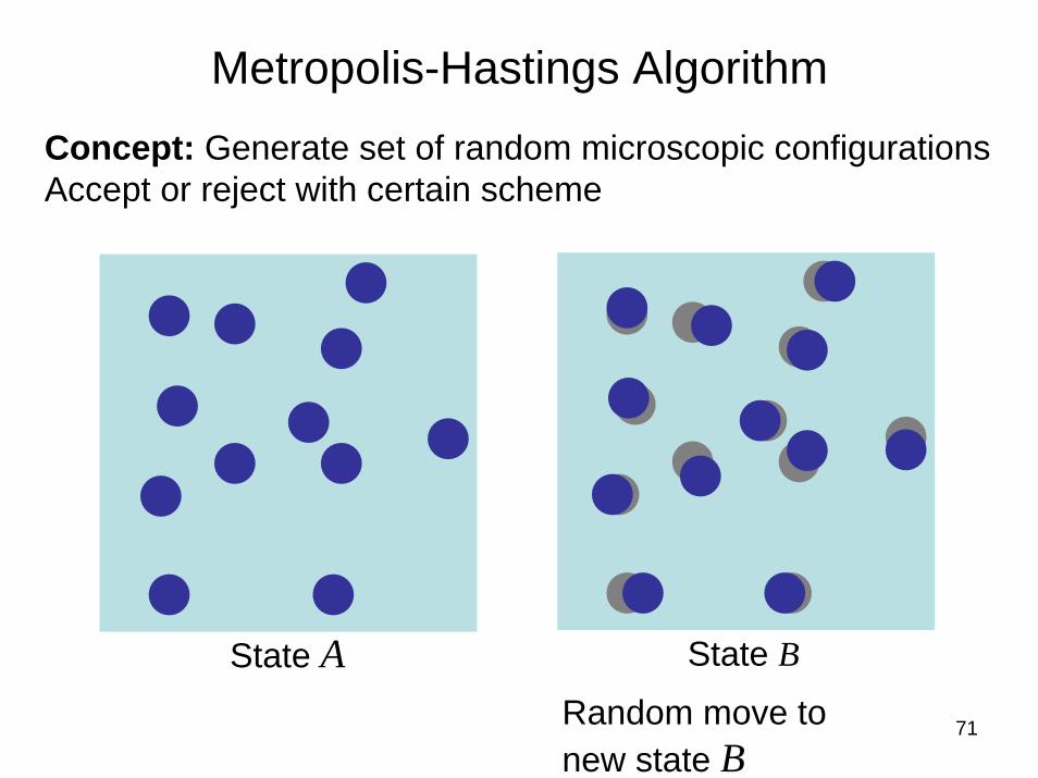
Metropolis-Hastings Algorithm
State A State B
Random move to new state B
Concept: Generate set of random microscopic configurationsAccept or reject with certain scheme
72
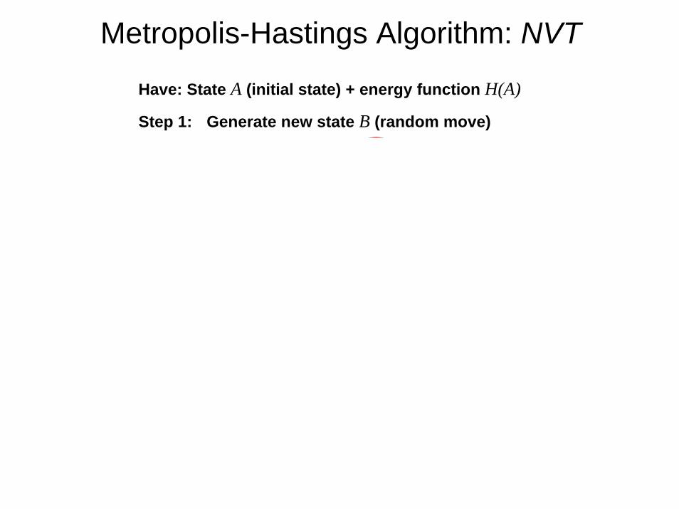
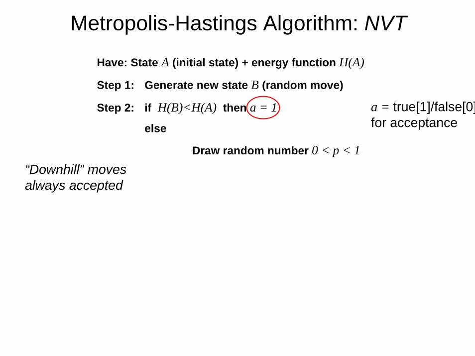
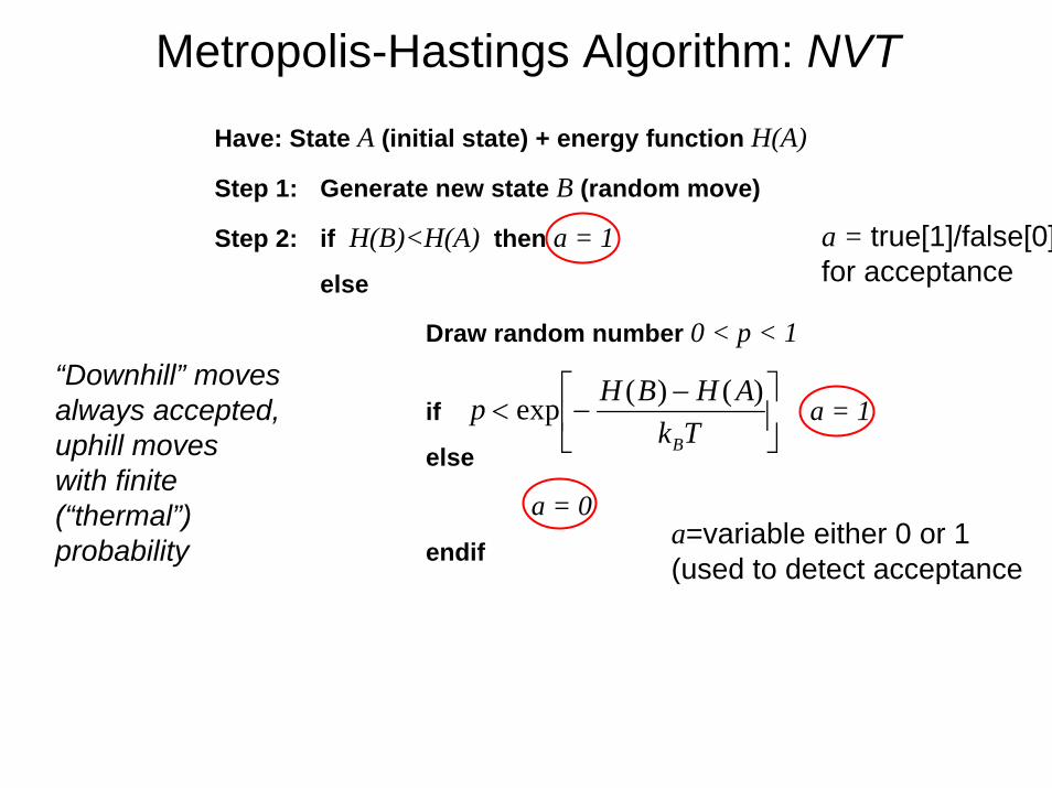
Have: State A (initial state) + energy function H(A)
Step 1: Generate new state B (random move)
Step 2: if H(B)<H(A) then a = 1
else
Draw random number 0 < p < 1
if a = 1
else
a = 0
endif
endif
Step 3: if a = 1 then accept state B
endif
Metropolis-Hastings Algorithm: NVT
∑=
>=<ANiA
iAN
A..1
)(1
⎥⎦
⎤⎢⎣
⎡ −−<
TkAHBHp
B
)()(exp
a = true/falsefor acceptance
“Downhill” moves always accepted, uphill moveswith finite (“thermal”) probability
a=variable either 0 or 1(used to detect acceptanceof state B when a=1)
73
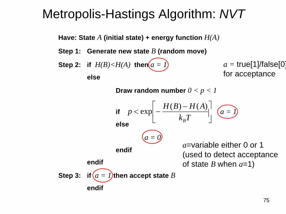
Have: State A (initial state) + energy function H(A)
Step 1: Generate new state B (random move)
Step 2: if H(B)<H(A) then a = 1
else
Draw random number 0 < p < 1
if a = 1
else
a = 0
endif
endif
Step 3: if a = 1 then accept state B
endif
Metropolis-Hastings Algorithm: NVT
∑=
>=<ANiA
iAN
A..1
)(1
⎥⎦
⎤⎢⎣
⎡ −−<
TkAHBHp
B
)()(exp
“Downhill” moves always accepted, uphill moveswith finite (“thermal”) probability
a=variable either 0 or 1(used to detect acceptanceof state B when a=1)
“Downhill” moves always accepted
a = true[1]/false[0]for acceptance
74
Have: State A (initial state) + energy function H(A)
Step 1: Generate new state B (random move)
Step 2: if H(B)<H(A) then a = 1
else
Draw random number 0 < p < 1
if a = 1
else
a = 0
endif
endif
Step 3: if a = 1 then accept state B
endif
Metropolis-Hastings Algorithm: NVT
∑=
>=<ANiA
iAN
A..1
)(1
⎥⎦
⎤⎢⎣
⎡ −−<
TkAHBHp
B
)()(exp
“Downhill” moves always accepted, uphill moveswith finite (“thermal”) probability
a=variable either 0 or 1(used to detect acceptanceof state B when a=1)
“Downhill” moves always accepted, uphill moveswith finite (“thermal”) probability
a = true[1]/false[0]for acceptance
75
Have: State A (initial state) + energy function H(A)
Step 1: Generate new state B (random move)
Step 2: if H(B)<H(A) then a = 1
else
Draw random number 0 < p < 1
if a = 1
else
a = 0
endif
endif
Step 3: if a = 1 then accept state B
endif
Metropolis-Hastings Algorithm: NVT
⎥⎦
⎤⎢⎣
⎡ −−<
TkAHBHp
B
)()(exp
a=variable either 0 or 1(used to detect acceptanceof state B when a=1)
a = true[1]/false[0]for acceptance
76
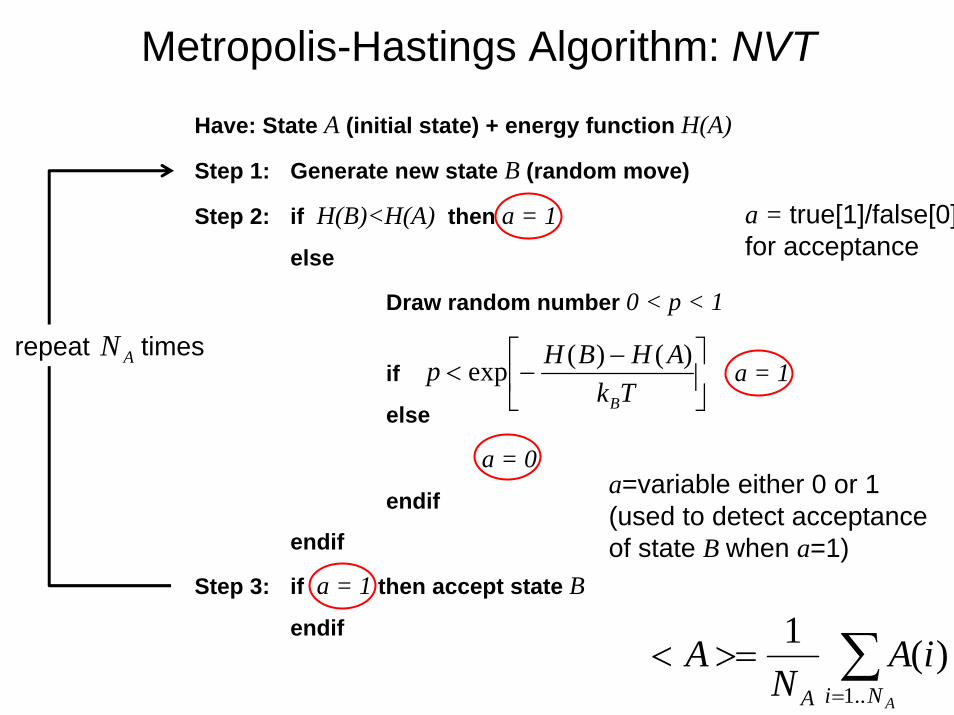
Have: State A (initial state) + energy function H(A)
Step 1: Generate new state B (random move)
Step 2: if H(B)<H(A) then a = 1
else
Draw random number 0 < p < 1
if a = 1
else
a = 0
endif
endif
Step 3: if a = 1 then accept state B
endif
repeat times
Metropolis-Hastings Algorithm: NVT
∑=
>=<ANiA
iAN
A..1
)(1
AN⎥⎦
⎤⎢⎣
⎡ −−<
TkAHBHp
B
)()(exp
a=variable either 0 or 1(used to detect acceptanceof state B when a=1)
a = true[1]/false[0]for acceptance
77
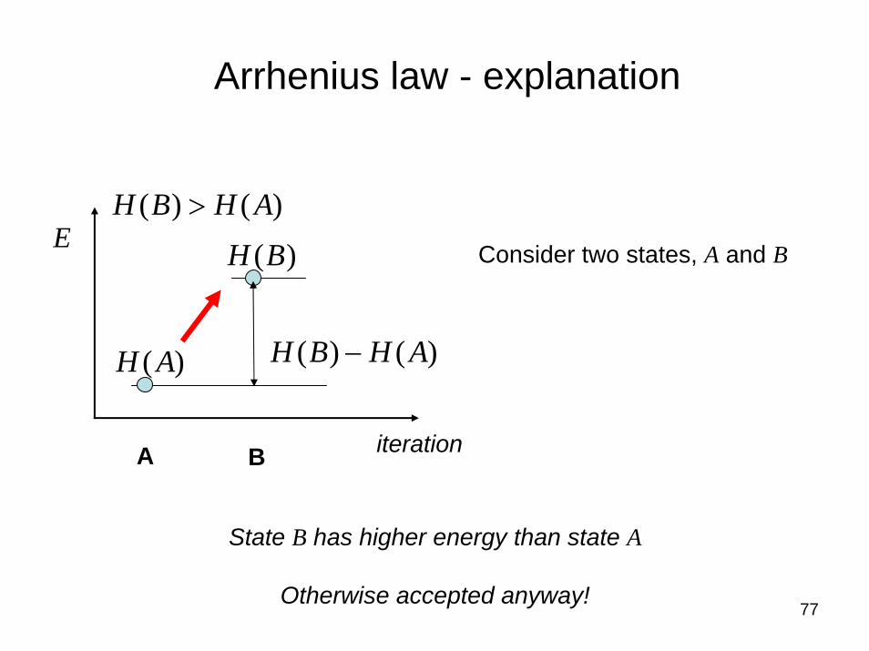
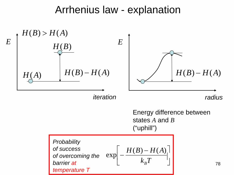
Arrhenius law - explanation
E
)()( AHBH −
iteration
)(AH
)(BH
)()( AHBH >
Consider two states, A and B
A B
State B has higher energy than state A
Otherwise accepted anyway!
78
Arrhenius law - explanation
E
)()( AHBH −
iteration
)(AH
)(BH)()( AHBH >
E
)()( AHBH −
radius
Energy difference betweenstates A and B(“uphill”)
Probabilityof successof overcoming the barrier at temperature T
⎥⎦
⎤⎢⎣
⎡ −−
TkAHBH
B
)()(exp
79
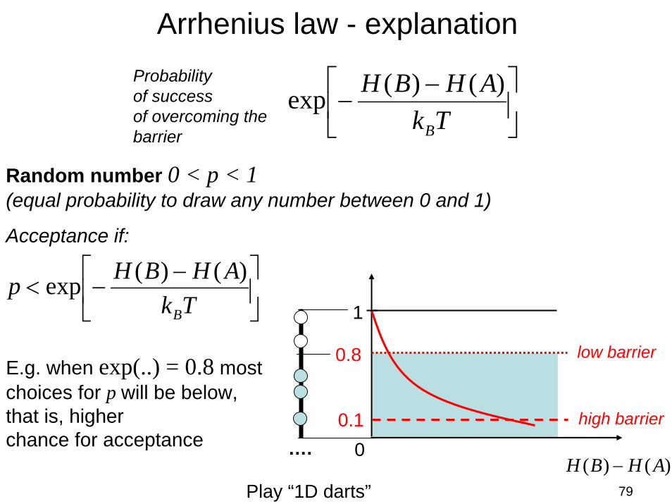
Arrhenius law - explanation
⎥⎦
⎤⎢⎣
⎡ −−<
TkAHBHp
B
)()(exp
⎥⎦
⎤⎢⎣
⎡ −−
TkAHBH
B
)()(exp
)()( AHBH −
1
0
0.8E.g. when exp(..) = 0.8 most choices for p will be below, that is, higherchance for acceptance
low barrier
high barrier0.1
Random number 0 < p < 1(equal probability to draw any number between 0 and 1)
Acceptance if:
Probabilityof successof overcoming the barrier
Play “1D darts”
….
80
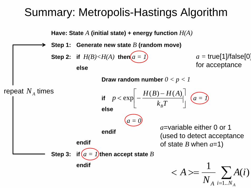
Have: State A (initial state) + energy function H(A)
Step 1: Generate new state B (random move)
Step 2: if H(B)<H(A) then a = 1
else
Draw random number 0 < p < 1
if a = 1
else
a = 0
endif
endif
Step 3: if a = 1 then accept state B
endif
repeat times
Summary: Metropolis-Hastings Algorithm
∑=
>=<ANiA
iAN
A..1
)(1
AN⎥⎦
⎤⎢⎣
⎡ −−<
TkAHBHp
B
)()(exp
a=variable either 0 or 1(used to detect acceptanceof state B when a=1)
a = true[1]/false[0]for acceptance
81
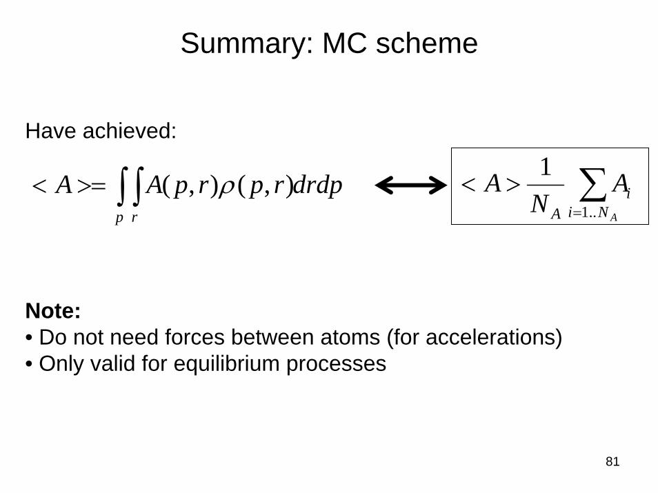
Summary: MC scheme
drdprprpAAp r∫ ∫>=< ),(),( ρ ∑
=
><ANi
iA
AN
A..1
1Have achieved:
Note:• Do not need forces between atoms (for accelerations)• Only valid for equilibrium processes
82
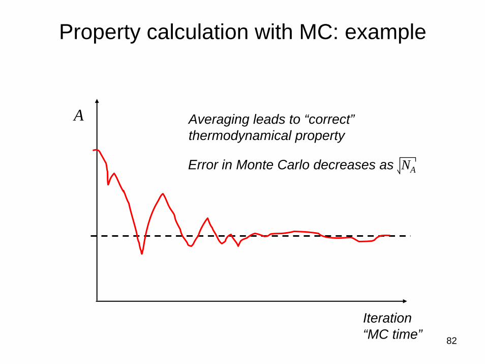
Property calculation with MC: example
A
Iteration“MC time”
Averaging leads to “correct”thermodynamical property
Error in Monte Carlo decreases as NA
83
Other ensembles/applications
Other ensembles carried out by modifying the acceptance criterion (in Metropolis-Hastings algorithm), e.g. NVT, NPT; goal is to reach the appropriate distribution of states according to the corresponding probability distributions
Move sets can be adapted for other cases, e.g. not just move of particles but also rotations of side chains(=rotamers), torsions, etc.
E.g. application in protein folding problem when we’d like to determine the 3D folded structure of a protein in thermal equilibrium, NVT
After: R.J. Sadus
84
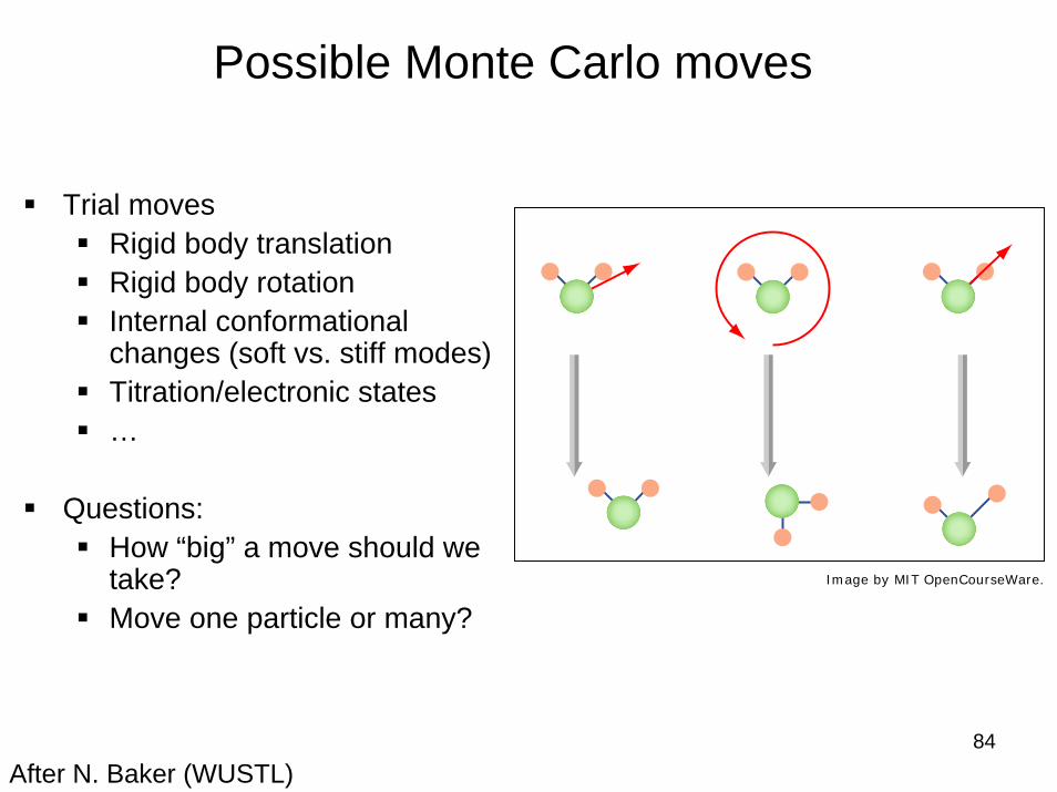
Possible Monte Carlo moves
Trial movesRigid body translationRigid body rotationInternal conformational changes (soft vs. stiff modes)Titration/electronic states…
Questions:How “big” a move should we take?Move one particle or many?
After N. Baker (WUSTL)
Image by MIT OpenCourseWare.
85
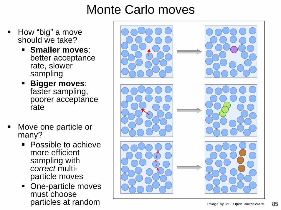
Monte Carlo moves
How “big” a move should we take?
Smaller moves: better acceptance rate, slower samplingBigger moves: faster sampling, poorer acceptance rate
Move one particle or many?
Possible to achieve more efficient sampling with correct multi-particle movesOne-particle moves must choose particles at random Image by MIT OpenCourseWare.

MIT OpenCourseWarehttp://ocw.mit.edu
3.021J / 1.021J / 10.333J / 18.361J / 22.00J Introduction to Modeling and SimulationSpring 2012
For information about citing these materials or our Terms of use, visit http://ocw.mit.edu/terms.