Propensity-Score-Based Methods versus MTE-Based … · Propensity-Score-Based Methods versus MTE...

Propensity-Score-Based Methods versus MTE-Based Methods

in Causal Inference

Xiang Zhou University of Michigan

Yu Xie

University of Michigan

Population Studies Center Research Report 11-747 December 2011

Direct all correspondence to Xiang Zhou or Yu Xie, Institute for Social Research, University of Michigan, 426 Thompson Street, Ann Arbor, MI 48106, USA; email: [email protected] or [email protected]. Financial support for this research was provided by the National Institutes of Health, Grant 1 R21 NR010856-01 and by the Population Studies Center at the University of Michigan, which receives core support from the National Institute of Child Health and Human Development, Grant R24HD041028. The authors benefitted from communications with Jennie Brand, James Heckman, and Ben Jann. The ideas expressed herein are those of the authors.

mailto:[email protected]

mailto:[email protected]

Propensity-Score-Based Methods versus MTE-Based Methods in Causal Inference 2

ABSTRACT

Since the seminal introduction of the propensity score by Rosenbaum and Rubin, propensity-score-based (PS-based) methods have been widely used for drawing causal inferences in the behavioral and social sciences. However, the propensity score approach depends on the ignorability assumption: there are no unobserved confounders once observed covariates are taken into account. For situations where this assumption may be violated, Heckman and his associates have recently developed a novel approach based on marginal treatment effects (MTE). In this paper, we (1) explicate consequences for PS-based methods when aspects of the ignorability assumption are violated; (2) compare PS-based methods and MTE-based methods by making a close examination of their identification assumptions and estimation performances; (3) illustrate these two approaches in estimating the economic return to college using data from NLSY 1979 and discuss discrepancies in results. When there is a sorting gain but no systematic baseline difference between treated and untreated units given observed covariates, PS-based methods can identify the treatment effect of the treated (TT). The MTE approach performs best when there is a valid and strong instrumental variable (IV).


1. Introduction

Since the seminal introduction of the propensity score by Rosenbaum and Rubin (1983),

propensity-score-based (PS-based) methods, including matching, stratification, and weighting,

have become a mainstay strategy for drawing causal inferences in the behavioral and social

sciences. By reducing a large array of confounding variables to a univariate measure that

preserves all the relevant information of potential confounders, the propensity score provides a

more efficient tool than covariate adjustment does for eliminating confounder bias. Furthermore,

social science researchers have recently utilized propensity score methods to study

heterogeneous treatment effects across individuals with different propensities of being treated.

For example, Brand and Xie (2010) recently found that those students who are least likely to

obtain a college education benefit most from college.

Like all other solutions to confounding problems in causal inference, the propensity score

approach is by no means a miracle cure. The primary limitation of this approach lies in the

impossibility of capturing unobserved individual and contextual confounders. In fact, the whole

justification of propensity-score-based methods hinges on the common “ignorability assumption”:

through control of a given set of relevant observed covariates, treatment status is assumed to be

independent of potential outcomes. This assumption is unverifiable, indeed unlikely to be true, in

practice. For instance, economic theory predicts that attainment of college education may be

selective because it may attract young persons who are motivated by economic gain from college

education (Willis and Rosen 1979; Carneiro, Heckman, and Vytlacil 2011). This example

illustrates the effect of “sorting on gain” that may not be captured by observed covariates such as

family background and cognitive abilities.

Despite the aforementioned limitation, PS-based methods are still widely used by

empirical researchers in a variety of disciplines. Not only is the propensity-score approach


simple and straightforward, but methods of addressing unobserved selection would require either

additional data unavailable to the researcher or strong assumptions implausible in a research

setting. However, the performance of PS-based methods is questionable when the ignorability

assumption breaks down. Although sensitivity analysis is usually employed to assess the

plausibility of findings (Harding 2003; DiPrete and Gangl 2004), systematic investigation is also

needed to directly examine the consequences for PS-based methods when ignorability is violated.

A related discussion can be found in Heckman and Navarro-Lozano (2004), who compared

matching, instrumental variables (IVs) and control functions in the estimation of economic

choice models. Blundell, Dearden, and Sianesi (2005) also compared least squares, matching,

control functions and IV from a methodological point of view within a common framework.

More recently, Shadish, Clark, and Steiner (2008) explored the performances of OLS adjustment

and propensity score adjustment with different sets of predictors in an experimental setting.

Inspired by these studies, this paper aims to provide another examination of PS-based methods in

a variety of plausible situations.

Our paper goes beyond PS-based methods by evaluating a structural approach, developed

by James Heckman and his associates, to situations in which the ignorability assumption is

violated (Heckman and Vytlacil 1999, 2001, 2005; Heckman, Urzua, and Vytlacil 2006a, 2006b).

Based on the building block of marginal treatment effect (MTE), this approach is comprehensive

and flexible in its ability to derive various parameters of interest within a single framework.

However, MTE-based methods have not been widely used in empirical research (for a few

exceptions, see Carneiro, Heckman, and Vytlacil 2011; Moffitt 2008; Tsai and Xie 2011), partly

due to its complexity and demands on data. In fact, the aforementioned literature suggests that

the utility of MTE hinges heavily on the validity of exclusion restriction as well as the strength


of instrumental variables.1 The properties of this approach are not yet well known when either

the exclusion restriction is violated or the instrumental variable is too “weak.”

In this paper, we evaluate and compare the widely adopted PS-based methods and the

less popular MTE-based approach, as follows. In Section 2, we revisit population heterogeneity

and two types of selection bias in causal inference, presenting propensity-score-based methods

and their implications in settings where the ignorability assumption is partially or completely

violated. In particular, we propose a PS-based method by modeling counterfactual outcomes as

nonparametric functions of the propensity score, which we call the “smoothing-difference

method.” In Section 3, we introduce the MTE-based approach as a remedy for situations where

the ignorability assumption may be violated. In Section 4, we compare PS-based methods and

MTE-based methods by examining their identification assumptions and estimation performances.

We use numerical simulation to explore (1) the relative efficiency of these two approaches when

both ignorability and exclusion restriction hold true, and (2) potential biases from using methods

based on the two approaches when neither ignorability nor exclusion restriction is guaranteed. In

Section 5, we illustrate both methods in analyzing the economic return to college education using

a sample of white males from the National Longitudinal Survey of Youth of 1979 (NLSY), and

discuss discrepancies in results. In Section 6 we conclude.

2. Ignorability and Propensity-Score-Based Methods

Population sciences, including economics, demography, epidemiology, psychology, and

sociology, treat individual-level variation as a part of reality subject to scientific inquiry, rather

than a mere nuisance or measurement error (Angrist and Kruger 1999; Ansari and Kamel 2000;

Bauer and Curran 2003; Greenland and Poole 1988; Heckman 2001, 2005; Heckman and Robb

1985; Heckman and Vytlacil 2005; Lubke and Muthen 2005; Manski 2007; Moffitt 1996;


Rothman and Greenland 1998; Winship and Morgan 1999; Xie 2007). The recognition of

inherent individual-level heterogeneity has important consequences for research designs in the

social sciences. Because individuals differ from one another and differ in their response to a

common treatment, results can vary widely depending on population composition.

The large methodological literature on causal inference using statistical methods

recognizes the importance of and consequently allows for population heterogeneity (Heckman

and Vytlacil 2005; Holland 1986; Manski 1995; Rubin 1974; Winship and Morgan 1999).

Suppose that a population, 𝑈, is being studied. Let 𝑌 denote an outcome variable of interest (its

realized value being 𝑦) that is a function for each member in 𝑈. Let us define treatment as an

externally induced intervention that can, at least in principle, be given to or withheld from a unit

under study. For simplicity, we consider only dichotomous treatments and use 𝐷 to denote the

treatment status (its realized value being 𝑑), with 𝐷 = 1 if a member is treated and 𝐷 = 0 if a

member is not treated. Let subscript i represent the ith member in 𝑈. We further denote 𝑦𝑖1as the

ith member’s potential outcome if treated (i.e., when di=1), and 𝑦𝑖0 as the ith member’s potential

outcome if untreated (i.e., when di=0). The framework for counterfactual reasoning in causal

inference (Heckman 2005; Holland 1986; Manski 1995; Morgan and Winship 2007; Rubin 1974;

Sobel 2000; Winship and Sobel 2004) states that we should conceptualize a treatment effect as

the difference in potential outcomes associated with different treatment states for the same

member in 𝑈:

𝛿𝑖 = 𝑦𝑖1 − 𝑦𝑖0, (1)

where δi represents the hypothetical treatment effect for the ith member.2 The fundamental

problem of causal inference (Holland 1986) is that, for a given unit i, we observe either 𝑦𝑖1 (if

di=1) or 𝑦𝑖0 (if di=0), but not both. Given this fundamental problem, how can we estimate


treatment effects? Holland describes two possible solutions: the “scientific solution” and the

“statistical solution.” The scientific solution capitalizes on homogeneity in assuming that all

members in U are the same, in either the treated state or the control state: 𝑦𝑖1 = 𝑦𝑗1 and 𝑦𝑖0 = 𝑦𝑗0,

where j ≠ i in U. This strong homogeneity assumption would enable a researcher to identify

individual-level treatment effects by as few as two cases in U. However, as we discussed above,

pervasive heterogeneity across units is the norm rather than the exception in a population science.

Thus, in general, the scientific solution has no practical value in the social and behavioral

sciences.

2.1. Quantit ies of Interest

For a population science, the statistical solution is a necessity. The statistical approach is to

compute quantities of interest that reveal treatment effects only at the group level. For example,

we may evaluate the average difference between a set of members in U that were randomly

selected for treatment and another set of members that were randomly selected for control. This

comparison yields a quantity that is called the average treatment effect (ATE):

ATE = 𝐸(𝑌1 − 𝑌0).

While ATE is defined for the whole population, the researcher may wish to focus on and define a

treatment effect for a well-defined subpopulation. For example, the treatment effect of the

treated (TT) refers to the average difference by treatment status among those individuals who are

actually treated:

TT = 𝐸(𝑌1 − 𝑌0|𝐷 = 1).

Analogously, the treatment effect of the untreated (TUT) refers to the average difference by

treatment status among those individuals who are not treated:

TUT = 𝐸(𝑌1 − 𝑌0|𝐷 = 0).


Although various statistical quantities of interest can easily be defined theoretically with the

statistical “solution,” estimating these quantities in social research can be very difficult, due to

two types of selection bias, a topic to be discussed in the next subsection.

2.2. Two Types of Selection Bias

In the preceding subsection, we established the need to conduct group-level comparisons for

causal inference, because causal inference is impossible at the individual level. The rationale is

to compare groups that are essentially comparable except for their treatment status. However,

due to population heterogeneity, there is no guarantee that the group that actually receives the

treatment is comparable, in observed and particularly in unobserved contextual and individual

characteristics, to the group that does not receive the treatment.3 Individuals may self-select into

treatment based on their anticipated monetary and nonmonetary benefits and costs of treatment.

To see this, let us partition the total population U into the subpopulation of the treated U1 (for

which D=1) and the subpopulation of the untreated U0 (for which D=0). We can thus decompose

the expectations for the two counterfactual outcomes as follows:

𝐸(𝑌1) = 𝐸(𝑌1|𝐷 = 1)𝑃(𝐷 = 1) + 𝐸(𝑌1|𝐷 = 0)𝑃(𝐷 = 0),

and

𝐸(𝑌0) = 𝐸(𝑌0|𝐷 = 1)𝑃(𝐷 = 1) + 𝐸(𝑌0|𝐷 = 0)𝑃(𝐷 = 0).

The issue of selection stems from the scenario

𝐸(𝑌1|𝐷 = 1) ≠ 𝐸(𝑌1|𝐷 = 0) ≠ 𝐸(𝑌1), (2)

and

𝐸(𝑌0|𝐷 = 1) ≠ 𝐸(𝑌0|𝐷 = 0) ≠ 𝐸(𝑌0). (3)

Note that what we observe from data are 𝐸�(𝑌1|𝐷 = 1),𝐸�(𝑌0|𝐷 = 0),𝑃�(𝐷 = 1), and 𝑃�(𝐷 = 0).

Due to inequalities (2) and (3), the simple-comparison estimator 𝐸�(Y1|𝐷 = 1) − 𝐸�(Y0|𝐷 = 0),


as a naive estimator for ATE, may be contaminated by selection bias. Denoting this estimator by

�̂�𝑛𝑎𝑖𝑣𝑒, we can decompose its expectation as follows:

𝐸��̂�𝑛𝑎𝑖𝑣𝑒� = 𝐸(𝑌1|𝐷 = 1) − 𝐸(𝑌0|𝐷 = 0)

= 𝐸(𝑌1 − 𝑌0|𝐷 = 1) + 𝐸(Y0|𝐷 = 1) − 𝐸(Y0|𝐷 = 0)

= TT + 𝐸(Y0|𝐷 = 1) − 𝐸(Y0|𝐷 = 0)

= ATE + (TT − ATE) + 𝐸(Y0|𝐷 = 1) − 𝐸(Y0|𝐷 = 0). (4)

From equation (4), we see two sources of selection bias:

1. The difference in average outcomes between the treatment and control groups if neither

group receives treatment: 𝐸(𝑌0|𝐷 = 1) − 𝐸(𝑌0|𝐷 = 0). We call this the “pre-treatment

heterogeneity bias” or “Type I selection bias.”

2. The difference in average treatment effects between the treated group and the entire

population. We call this the “treatment-effect heterogeneity bias” or “Type II selection

bias.” There is treatment-effect heterogeneity bias if and only if TT ≠ ATE.

We now illustrate the two different sources of selection bias with two concrete examples.

First, pre-school children from poor families are selected into Head Start programs and thus

would compare unfavorably to other children who do not attend Head Start programs without an

adequate control for family socioeconomic resources (Xie 2000). Second, economic theory

predicts that attainment of college education may be selective because it may attract young

persons who are more motivated than their peers to gain from college education (Willis and

Rosen 1979). While the first example reflects the importance of pre-treatment heterogeneity bias

that may be represented by “covariates” or “fixed effects,” the second example underscores the

possibility of treatment-effect heterogeneity bias – sorting on the treatment effects – which

cannot be captured in general by “covariates” or “fixed effects.”


2.3. The Assumption of Ignorabil ity

With data from observational studies, where subjects have made their own choices regarding the

treatment status, the two types of selection bias cannot be ignored in general. To overcome

potential biases resulting from non-randomness in treatment assignment, a natural idea is to

control for observed pre-treatment covariates. While it is not possible for a researcher to claim

that he or she has controlled for almost all of the variables that may affect the outcome, it is more

plausible to assume that the researcher has controlled for almost all of the relevant pre-treatment

covariates that may affect both the treatment assignment and the outcome, a subset of all the

variables affecting the outcome. Of course, only the covariates that meet the condition of

affecting both the treatment assignment and the outcome may potentially confound the observed

relationship between treatment and outcome (Rubin 1997). Thus, if we assume that all these

relevant pre-treatment variables are observed, the treatment status will be independent of

potential outcomes through control of these covariates. This conditional independence

assumption is called “ignorability,” “unconfoundedness,” or “selection on observables.” If we let

𝑿 be the vector of these observed covariates, the ignorability assumption states:

(𝑌1,𝑌0) ∥ 𝐷|𝑿. (5)

Because we can never be sure after inclusion of which covariates equation (5) would hold true,

the ignorability condition is always held as an assumption, indeed an unverifiable assumption.

Substantive knowledge about the subject matter needs to be brought in before a researcher can

entertain the ignorability assumption. Measurement of theoretically meaningful confounders

makes ignorability tentatively plausible, but not necessarily true. However, the researcher can

always consider the ignorability assumption and then assess its plausibility in a concrete setting


through sensitivity or auxiliary analyses (Cornfield et al. 1959; DiPrete and Gangl 2004; Harding

2003; Rosenbaum 2002; Xie and Wu 2005).

If the ignorability assumption (5) holds true, we can change inequalities (2) and (3) into

two equalities by conditioning on 𝑿: 3F

4

𝐸(𝑌1|𝐷 = 1,𝑿) = 𝐸(𝑌1|𝐷 = 0,𝑿) = 𝐸(𝑌1|𝑿); (6)

𝐸(𝑌0|𝐷 = 1,𝑿) = 𝐸(𝑌0|𝐷 = 0,𝑿) = 𝐸(𝑌0|𝑿). (7)

For now, we are concerned only with identification and postpone inference issues to a later

discussion. Let us define quantities of interest for causal inference, conditioning on 𝑿, as

follows:

ATE(𝑿) = 𝐸(𝑌1 − 𝑌0|𝑿),

TT(𝑿) = 𝐸(𝑌1 − 𝑌0|𝐷 = 1,𝑿),

TUT(𝑿) = 𝐸(𝑌1 − 𝑌0|𝐷 = 0,𝑿).

Similarly, we define the naive estimator conditioning on 𝑿 as:

�̂�𝑛𝑎𝑖𝑣𝑒(𝑿) = 𝐸�(𝑌1|𝐷 = 1,𝑿) − 𝐸�(𝑌0|𝐷 = 0,𝑿).

Then equations (6) and (7) imply the following identity

𝐸 ��̂�𝑛𝑎𝑖𝑣𝑒(𝑿)� = ATE(𝑿) = TT(𝑿) = TUT(𝑿). (8)

As a result, the ignorability assumption enables the naive estimator to identify all the

aforementioned treatment parameters through control of 𝑿. Conditioning on 𝑿, however, can be

difficult in applied research due to the “curse of dimensionality.” Rosenbaum and Rubin (1983,

1984) show that, when the ignorability assumption holds true, it is sufficient to condition on the

propensity score as a function of 𝑿. That is to say, relation (5) implies:

(𝑌1,𝑌0) ∥ 𝐷|𝑃(𝐷 = 1|𝑿),


where 𝑃(𝐷 = 1|𝑿) is the propensity score, the conditional probability of treatment given all the

relevant information in covariates 𝑿. In other words, only through the propensity score 𝑃(𝐷 =

1|𝑿) may covariates 𝑿 confound the observed relationship between treatment 𝐷 and outcome 𝑌.

2.4. Propensity-Score-Based Methods

From above, we know that it is sufficient to condition on the propensity score 𝑃(𝐷 = 1|𝑿) as

long as the ignorability assumption is satisfied. In empirical settings, however, the propensity

score first needs to be estimated. Since a fully nonparametric estimation of the propensity score

would also suffer from the curse of dimensionality, the estimation is conventionally

accomplished by a logit or probit regression. From here on, we denote by 𝑝 the propensity score

and by �̂�𝑛𝑎𝑖𝑣𝑒(𝑝) the naive estimator of treatment effect conditional on 𝑝. Note that �̂�𝑛𝑎𝑖𝑣𝑒(𝑝)

here is a function of 𝑝, but not necessarily a linear function of 𝑝. There are a variety of different

methods of constructing �̂�𝑛𝑎𝑖𝑣𝑒(𝑝). Below, we briefly discuss what we call the “smoothing-

difference method,” through fitting two nonparametric functions for 𝐸(𝑌1|𝑝) and 𝐸(𝑌0|𝑝). The

smoothing-difference method consists of the following four steps:

1. From observed 𝑌1 and 𝑌0 and estimated propensity score �̂�, fit two univariate functions

of 𝑝 , 𝑓1(𝑝) and 𝑓0(𝑝) to approximate 𝐸(𝑌1|𝑝) and 𝐸(𝑌0|𝑝).

2. Use 𝑓1(𝑝) and 𝑓0(𝑝) to predict counterfactual outcomes 𝑌𝑖1 and 𝑌𝑖0 for each individual 𝑖

in the sample.

3. Obtain the estimated treatment effect 𝛿𝑖 for each individual i by taking the difference

between the predicted counterfactual outcomes.

4. Average estimated 𝛿𝑖 over the entire sample as the estimate of ATE, or over a specific

subsample to estimate a corresponding group-level causal effect. For example, we may

estimate TT by averaging 𝛿𝑖 over those subjects who are actually treated.


Note that in the first step, 𝑓1(𝑝) and 𝑓0(𝑝) could be fitted via different estimation

methods. One simple possibility is to fit two linear models of 𝑌1 and 𝑌0 on 𝑝 through simple

least squares. However, this strategy imposes too strong a parametric assumption concerning the

relationship between the outcome variables and the propensity score. To relax this highly

restrictive parametric assumption, we propose to fit two smoothing splines (Hastie, Tibshirani,

and Friedman 2008) of 𝑌1 and 𝑌0 on 𝑝 with the smoothing parameter determined by generalized

cross validation or some other criterion.5 We will adopt this approach in our simulation studies in

Section 4, as well as the analysis of NLSY data in Section 5.

Other propensity-score-based methods include matching, stratification, and weighting, all

of which have been widely used in empirical research. Compared to these traditional methods,

our smoothing-difference method has two distinct advantages.6 First and foremost, it preserves

information pertaining to the heterogeneity across subjects with different propensity scores. For

example, the research interest may lie in the trend of Δ𝑓(𝑝), i.e., 𝑓1(𝑝) − 𝑓0(𝑝), which

characterizes how the treatment effect varies across subjects with different propensities of being

treated (Brand and Xie 2010; Xie, Brand, and Jann 2012; Xie and Wu 2005). Such a pattern may

identify population subgroups that benefit most from the treatment, thus offering meaningful

policy implications. On the other hand, the researcher may be interested in the trends of the

outcome as a function of the propensity score among either treated or untreated subjects, i.e.,

𝑓0(𝑝) 𝑜𝑟 𝑓1(𝑝), which could not be extracted from results using matching or stratification

methods. As we will illustrate in Section 5, these trends can enhance our understanding of the

social processes that may be masked by an exclusive attention to the estimation of causal effects.

In addition, after we pool information through nonparametric regressions across adjacent cases

within either treated or untreated groups, we are able to derive the estimated treatment effect


𝛿𝑖 for each individual 𝑖, before we calculate any group-level treatment effect through averaging

over an appropriate subsample.

2.5. Decomposition of Ignorabil ity

Equations (4) and (8) reveal that, under the ignorability assumption, controlling for observed

covariates removes both types of selection bias. This suggests that the ignorability assumption

should contain two components corresponding to the two types of bias. Indeed, ignorability

expressed as relation (5) can be rewritten as

(𝑌0,𝑌1 − 𝑌0) ∥ 𝐷|𝑿.

This expression illustrates the two conditions underlying the ignorability assumption:

Condition 1

𝑌0 ∥ 𝐷|𝑿,

i.e., given observed covariates, treatment status is independent of the baseline outcome;

Condition 2

𝑌1 − 𝑌0 ∥ 𝐷|𝑿,

i.e., given observed covariates, treatment status is independent of the treatment effect. We may

call Condition 1 the ignorability of Type I selection bias, and Condition 2 the ignorability of

Type II selection bias. The ignorability assumption, in essence, means the ignorability of both

Type I selection bias and Type II selection bias.

As mentioned in Section 2.3, Rosenbaum and Rubin (1983) derive the sufficiency of

propensity score under the assumption of complete ignorability for eliminating confounding bias:

If (𝑌1,𝑌0) ∥ 𝐷|𝑿, then (𝑌1,𝑌0) ∥ 𝐷|𝑃(𝐷 = 1|𝑿).

Indeed, the proof provided by Rosenbaum and Rubin (1983) implies the following two

propositions:


Proposition 1

If 𝑌0 ∥ 𝐷|𝑿 , then 𝑌0 ∥ 𝐷|𝑃(𝐷 = 1|𝑿); (9)

Proposition 2

If 𝑌1 − 𝑌0 ∥ 𝐷|𝑿 , then 𝑌1 − 𝑌0 ∥ 𝐷|𝑃(𝐷 = 1|𝑿). (10)

As before, we denote by 𝑝 the propensity score 𝑃(𝐷 = 1|𝑿) and by �̂�𝑛𝑎𝑖𝑣𝑒(𝑝) the naive

estimator of treatment effect conditional on 𝑝. In light of equation (4), the expectation of

�̂�𝑛𝑎𝑖𝑣𝑒(𝑝) could be decomposed as follows:

𝐸(�̂�𝑛𝑎𝑖𝑣𝑒(𝑝)) = 𝐸(Y1|𝐷 = 1,𝑝) − 𝐸(Y0|𝐷 = 0,𝑝)

= 𝐸(𝑌1 − 𝑌0|𝐷 = 1, 𝑝) + 𝐸(Y0|𝐷 = 1,𝑝) − 𝐸(Y0|𝐷 = 0,𝑝)

= TT(𝑝) + 𝐸(Y0|𝐷 = 1,𝑝) − 𝐸(Y0|𝐷 = 0,𝑝)

= ATE(𝑝) + TT(𝑝) − ATE(𝑝) + 𝐸(Y0|𝐷 = 1,𝑝) − 𝐸(Y0|𝐷 = 0,𝑝). (11)

Equation (11), combined with Propositions 1 and 2, shows that the naive estimator

�̂�𝑛𝑎𝑖𝑣𝑒(𝑝) identifies different quantities under different conditions. First, if Condition 1 holds

true, Type I selection bias thus becomes ignorable, i.e.,

𝐸(Y0|𝐷 = 1, 𝑝) = 𝐸(Y0|𝐷 = 0,𝑝).

In this scenario, we have

𝐸(�̂�𝑛𝑎𝑖𝑣𝑒(𝑝)) = TT(𝑝).

Second, if Condition 2 holds true, Type II selection bias becomes ignorable, i.e.,

𝐸(𝑌1 − 𝑌0|𝑝,𝐷 = 1) = 𝐸(𝑌1 − 𝑌0|𝑝),

or

TT(𝑝) = ATE(𝑝).

In this scenario, we have

𝐸(�̂�𝑛𝑎𝑖𝑣𝑒(𝑝)) = ATE(𝑝) + 𝐸(Y0|𝐷 = 1, 𝑝) − 𝐸(Y0|𝐷 = 0,𝑝).


From the above discussion, we conclude that:

1. If the ignorability of Type I selection bias (i.e., Condition 1) holds true, the naive

estimator conditional on the propensity score, �̂�𝑛𝑎𝑖𝑣𝑒(𝑝), confronts only Type II

selection bias (treatment-effect heterogeneity bias), i.e., TT(𝑝) ≠ ATE(𝑝). However, if

our quantity of interest is TT rather than ATE, �̂�𝑛𝑎𝑖𝑣𝑒(𝑝) is an unbiased estimator.

2. If the ignorability of Type II selection bias (i.e., Condition 2) holds true, the naive

estimator conditional on the propensity score, �̂�𝑛𝑎𝑖𝑣𝑒(𝑝), is subject only to Type I

selection bias (pre-treatment heterogeneity bias), i.e., 𝐸(Y0|𝐷 = 1, 𝑝) ≠ 𝐸(Y0|𝐷 =

0, 𝑝).7

3. Marginal-Treatment-Effect-Based Approach

So far, we have seen that propensity-score-based methods are subject to biases when the

ignorability assumption is violated. Unfortunately, the ignorability assumption can never be

verified. What recourse is available to a researcher who finds the ignorability assumption

implausible in a research setting? In this section, we introduce the marginal treatment effect

(MTE) approach developed by Heckman and his associates (Heckman and Vytlacil 1999, 2001,

2005; Heckman, Urzua, and Vytlacil 2006a, 2006b). Essentially, these researchers show that

unbiased estimation of a wide range of treatment parameters (including ATE, TT and TUT) can

be obtained through different weighted averages of MTE (Björklund and Moffitt 1987). MTE

could be estimated either parametrically or semi-parametrically. In the following, we briefly

review this class of methods, under the heading of “MTE-based approach.”


3.1. The Definit ion of Marginal Treatment Effect

It is most convenient to explicate the MTE-based approach with three equations: outcome

equations under two counterfactual regimes (D=0, D=1) and a treatment selection equation. In

writing out each of the equations, we assume separability of the outcome variable into a

structural component due to a linear function of pre-treatment covariates and residual

components due to unobserved variables:8

𝑌0 = 𝜷𝟎′ 𝑿 + 𝜖 ,

𝑌1 = 𝜷𝟏′ 𝑿 + 𝜖 + 𝜂.

Here, corresponding to our decomposition of the two sources of ignorability, the error term 𝜖

captures the unobserved variables that affect only the baseline outcome, while the error term 𝜂

represents the unobserved variables that affect only units that are treated. Thus, the treatment

effect contains both the structural component (𝜷𝟎′ 𝑿 versus 𝜷𝟏′ 𝑿) and the residual component 𝜂.

This setup changes equation (1) so that heterogeneous treatment effect can be written in a

structural form:

𝛿(𝑿) = 𝑌1(𝑿) − 𝑌0(𝑿) = (𝜷𝟏 − 𝜷𝟎)′𝑿 + 𝜂.

Note that the treatment effect 𝛿 depends on covariates 𝑿. If we denote by 𝑌 the observed

outcome and by 𝐷 the treatment status, the above model could be written in the notation of

switching regression models:

𝑌 = (1 −𝐷)𝑌0 + 𝐷𝑌1

= 𝑌0 + 𝐷(𝑌1 − 𝑌0)

= 𝜷𝟎′ 𝑿 + (𝜷𝟏 − 𝜷𝟎)′𝑿𝐷 + 𝜖 + 𝜂𝐷.

We further specify a model for selection into treatment. Let 𝐷∗ be the latent tendency to

be treated:

𝐷∗ = 𝜸′𝒁 − 𝑉, (12)

𝐷 = 1(𝐷∗ > 0).


Here, 𝒁 is a vector of variables that predict the treatment probability, γ is a vector of coefficients,

and 𝑉 is a latent random variable representing disturbance. As in standard regression models, we

assume that error terms (𝜖, 𝜂,𝑉) have zero means and are jointly independent of 𝑿 and 𝒁. In

practice, 𝒁 consists of all predictors of treatment probability, including all the components in 𝑿

as well as some additional variables that predict only the treatment status 𝐷. These additional

variables are also called instrumental variables (IVs). The assumption that IVs affect only the

treatment status 𝐷 but not the outcome variable 𝑌 directly is called the exclusion restriction.

We can easily rewrite the treatment selection model (12) in the following form

𝐷∗� = 𝑝(𝒁) − 𝑈𝐷

𝐷 = 1�𝐷∗� > 0�,

where 𝑝(𝒁) = 𝑃(𝐷 = 1|𝒁) = 𝐹𝑉(𝜸′𝒁) denotes the propensity score of being treated given 𝒁 and

𝑈𝐷 = 𝐹𝑉(𝑉) follows a standard uniform distribution on [0,1]. 𝑈𝐷 represents a catch-all

unobserved selection component, interpretable as the level of unobserved resistance to receiving

treatment, normalized between 0 and 1. We see that 𝒁 enters the treatment selection model only

through the propensity score 𝑝(𝒁).

Based on the above specification of the outcome models and treatment selection model,

we define the Marginal Treatment Effect (MTE) as follows:

MTE(𝒙,𝑢𝐷) = 𝐸(𝛿|𝑿 = 𝒙,𝑈𝐷 = 𝑢𝐷)

= 𝐸((𝜷𝟏 − 𝜷𝟎)′𝒙 + 𝜂|𝑿 = 𝒙,𝑈𝐷 = 𝑢𝐷)

= (𝜷𝟏 − 𝜷𝟎)′𝒙 + 𝐸�𝜂�𝑉 = 𝐹𝑉−1(𝑢𝐷)�. (13)

Thus, MTE is essentially the expected treatment effect conditional on observed covariates

𝑿 = 𝒙 as well as the unobserved selection component 𝑈𝐷 = 𝑢𝐷.


As mentioned above, Heckman, Urzua, and Vytlacil (2006a, 2006b) have shown that

group-level treatment effects such as ATE and TT can be expressed as weighted averages of

MTE(𝒙,𝑢𝐷).9 However, the estimation of MTE(𝒙,𝑢𝐷) is not straightforward since neither the

counterfactual outcome nor the latent variable 𝑢𝐷 is observed. Now we briefly sketch the two

approaches to estimating MTE: (1) the parametric method, and (2) the semi-parametric method.

3.2. Parametric and Semi-parametric Estimation of MTE

First we write out the expectation of the observed outcome 𝑌 given covariates 𝑿 = 𝒙 and the

propensity score 𝑝(𝒁) = 𝑝:

𝐸(𝑌|𝑿 = 𝒙,𝑝(𝒁) = 𝑝) = 𝐸(𝜷𝟎′ 𝑿 + (𝜷𝟏 − 𝜷𝟎)′𝑿𝐷 + 𝜖 + 𝜂𝐷|𝑿 = 𝒙,𝑝(𝒁) = 𝑝)

= 𝜷𝟎′ 𝒙 + (𝜷𝟏 − 𝜷𝟎)′𝒙𝑝 + 𝐸(𝜂|𝐷 = 1, 𝑝(𝒁) = 𝑝)𝑝

= 𝜷𝟎′ 𝒙 + (𝜷𝟏 − 𝜷𝟎)′𝒙𝑝 + 𝐸(𝜂|𝑉 < 𝐹𝑉−1(𝑝))𝑝

= 𝜷𝟎′ 𝒙 + (𝜷𝟏 − 𝜷𝟎)′𝒙𝑝 + ∫ 𝐸(𝜂|𝑉 = 𝐹𝑉−1(𝑢𝐷))𝑑𝑢𝐷𝑝0 . (14)

Incorporating equation (13), the above expression can be simplified:

𝐸(𝑌|𝑿 = 𝒙,𝑝(𝒁) = 𝑝) = 𝜷𝟎′ 𝒙 + ∫ MTE(𝒙,𝑢𝐷)𝑑𝑢𝐷𝑝0 .

Differentiating the above equation with respect to 𝑝, we obtain MTE:

MTE(𝒙,𝑝) = 𝜕𝐸(𝑌|𝑿=𝒙,𝑝(𝒁)=𝑝)𝜕𝑝

. (15)

This expression relates MTE(𝒙,𝑝) to 𝐸(𝑌|𝑿 = 𝒙,𝑝(𝒁) = 𝑝) and thus provides a possible route

for estimating MTE.

In general, the third term in equation (14), ∫ 𝐸(𝜂|𝑉 = 𝐹𝑉−1(𝑢𝐷))𝑑𝑢𝐷𝑝0 , is an unknown

function of 𝑝. However, if we assume that error terms (𝜖, 𝜂,𝑉) follow a joint Gaussian

distribution 𝑁(0,𝛴), 𝐸(𝑌|𝑿 = 𝒙,𝑝(𝒁) = 𝑝) would become a linear combination of 𝒙, 𝒙𝑝 and

𝜙(𝛷−1(𝑝)).


Accordingly, the expression of MTE reduces to

MTE(𝒙,𝑢𝐷) = (𝜷𝟏 − 𝜷𝟎)′𝒙 + 𝜎𝜂𝑉Φ−1(𝑢𝐷),

where 𝜎𝜂𝑉 represents the covariance between 𝜂 and 𝑉. With this parametric specification, we

can estimate its unknown parameters (𝜷𝟏,𝜷𝟎,𝜎𝜂𝑉) via maximum likelihood. This is the

parametric MTE-based method, which is also called the “control function approach.” In fact,

given the parametric assumption, identification of MTE(𝒙,𝑢𝐷) is theoretically possible without

IVs.

In empirical settings, the assumption of joint normality is rarely justifiable. This

motivated Heckman, Urzua, and Vytlacil (2006b) to develop a semi-parametric method to

identify MTE(𝒙,𝑝), using equation (15), after first estimating equation (14) under more flexible

assumptions. Their method involves four steps10:

1. Fit local linear regressions of 𝑌, 𝑿, and 𝑿𝑝 on 𝑝 and extract their residuals 𝑅𝑌,𝑹𝑿,𝑹𝑿𝑝.

2. Regress 𝑅𝑌 on 𝑹𝑿 and 𝑹𝑿𝑝 using least squares to estimate the parametric component of

equation (14), i.e., 𝜷𝟎 and 𝜷𝟏 − 𝜷𝟎, and denote its residuals by 𝑅𝑌∗ .

3. Regress 𝑅𝑌∗ on 𝑝 using standard nonparametric techniques (such as local polynomial

regression) to model the third term in equation (14) as well as its derivative, i.e.,

𝐸�𝜂�𝑉 = 𝐹𝑉−1(𝑝)�.

4. Construct MTE(𝒙,𝑢𝐷), expressed in equation (13), using 𝜷𝟏� − 𝜷𝟎� from Step 2 and the

estimate of 𝐸�𝜂�𝑉 = 𝐹𝑉−1(𝑝)� from Step 3.

Appendix A provides our implementation of these procedures in R for estimating returns to

college with a sample of white males from NLSY79.

Since this method capitalizes on the net relationship of 𝐸(𝑌|𝑿 = 𝒙,𝑝(𝒁) = 𝑝) with 𝑝(𝒁)

after all covariates in 𝑿 are controlled for, the presence of at least a valid instrumental variable in


𝒁 is indispensable for identification. For this reason, the semi-parametric approach is also called

the “local instrumental variable” (LIV) method. In spite of its flexibility, the LIV method has

not been widely adopted in empirical research, due partly to its high data demand pertaining to

IVs. Although a detailed discussion on the asymptotic variance of the maximum likelihood

estimator for the parametric MTE method can be found in Heckman (1979) and Puhani (2000),

statistical properties of the semi-parametric LIV method are not yet well known to a wider

research community.11 This motivates us to evaluate the performance of MTE-based methods

through numerical simulation.

4. Evaluation of Different Methods

4.1. Assumptions for Identification

The preceding discussion indicates that different methods require different assumptions to

identify group-level treatment effects. Table 1 summarizes the assumptions that are required for

the PS-based methods, the parametric MTE-based method, and the semi-parametric MTE-based

method to identify ATE and TT. Generally speaking, both the PS-based and MTE-based

methods rely on strong and unverifiable assumptions, the former on ignorability, and the latter on

exclusion restriction or the distribution of error terms. In particular, several facts deserve our

attention. First, as we note in Section 2, the applicability of propensity-score-based methods is

not limited to settings in which complete ignorability is satisfied. As long as the ignorability of

Type I selection bias is satisfied, i.e., there is no systematic baseline difference between treated

and untreated units given observed covariates, the PS-based models yield good estimates of TT,

even in the presence of a heterogeneous treatment effect bias.


Table 1: Assumptions for Identification

Method Exclusion Restriction

(A valid IV)

Distributional Form of Error Terms

Ignorability Assumption

PS-Based Methods

No No Yes

Parametric MTE

No Yes No

Semi-parametric MTE (LIV) Yes No No

Notes: For the parametric MTE-based method, multivariate normality is conventionally assumed for error terms. For PS-based methods, when the parameter of interest is TT, only the ignorability of Type I selection bias is necessary.

Second, in contrast to the semi-parametric LIV approach, the parametric MTE-based

method requires the assumption of joint normality for error terms. Although in principle the

parametric MTE method does not need an instrumental variable for identification, identification

based on the parametric distribution is weak. In practice, availability of IVs that satisfy the

exclusion restriction assumption would greatly improve the efficiency of the ML estimation,12 a

facet of the MTE-based methods examined through numerical simulation in the next subsection.

In comparison to the PS-based methods, the MTE-based methods require a more explicit

micro-level model. From the discussion in Section 3.2, we see that the expression of MTE in

equation (13) requires the separability of observables and unobservables in the outcome

equations. Also, to estimate the parametric component of the model, we need to specify a

functional form (such as linearity) to characterize the dependence of 𝑌0 and 𝑌1 on 𝑿. For the

PS-based methods, however, the assumption of ignorability enables us to model counterfactual

outcomes (or treatment effects) along the single dimension of propensity score. As this can be

conducted in a purely nonparametric manner (as is commonly done in practice), the PS-based

methods do not require an explicit model specification (except for the propensity score model).


Ultimately, a choice between the PS-based methods versus the MTE-based methods is

driven by the plausibility of the ignorability assumption versus the exclusion restriction

assumption. If we suspect violation of ignorability but have valid IVs, the MTE-based approach

is preferable to the PS-based methods. However, as exclusion restriction is also a strong and

unverifiable assumption, determining its degree of plausibility requires substantial knowledge in

an actual research setting. If, however, we have no satisfactory instruments that would satisfy the

exclusion restriction but have sufficient information on relevant individual and contextual

characteristics so that the ignorability assumption becomes plausible, the PS-based approach is a

reasonable choice.

In the above discussion, the general guideline is quite clear when one assumption is more

plausible than the other. What, however, happens if the ignorability and the exclusion restriction

assumptions are equally plausible -- or equally implausible? In the rest of this section, we

examine the performances of different methods for the following two scenarios: (1) when both

the ignorability and the exclusion restriction assumptions hold true; (2) when both the

ignorability and exclusion restriction assumptions break down.

4.2. When Both Ignorability and Exclusion Restriction Hold True

As Table 1 shows, when both the ignorability and the exclusion restriction assumptions hold

true, both the PS-based methods and the MTE-based methods can correctly identify group-level

causal effects (as long as the data-generating model is rightly specified). In this case, they both

provide estimates of ATE and TT that are asymptotically unbiased. Nonetheless, their statistical

efficiency may differ. Although estimation uncertainty may converge to zero as sample size goes

to infinity, we cannot avoid the limitation of sample size in empirical research. At present, we

know little about the asymptotic variance of the estimators produced by the semi-parametric


MTE method. It is therefore of practical relevance for us to explore the statistical efficiency of

the methods being evaluated in this paper.

To achieve this end, we utilize simulated data. First, we generate data through the two

potential outcome models and the treatment selection model described in Section 3:

𝑌0 = 𝛽00 + 𝛽01𝑋 + 𝜖

𝑌1 = 𝛽10 + 𝛽11𝑋 + 𝜖 + 𝜂

𝐷∗ = 𝛾0 + 𝛾1𝑋 + 𝛾2𝑍 − 𝑉

𝐷 = 1(𝐷∗ > 0),

with the following parameterization:

𝜷𝟎 = [𝛽00,𝛽01] = [0, 1], 𝜷𝟏 = [𝛽10,𝛽11] = [3,2]

𝜸 = [𝛾0,𝛾1,𝛾2] = [0, 𝛾1,𝛾2], 𝛾12 + 𝛾22 = 1

𝑋,𝑍~𝑁(0,1), 𝑋 ∥ 𝑍

𝜖, 𝜂,𝑉~𝑁(0,1), 𝜖 , 𝜂,𝑉 𝑚𝑢𝑡𝑢𝑎𝑙𝑙𝑦 𝑖𝑛𝑑𝑒𝑝𝑒𝑛𝑑𝑒𝑛𝑡

𝜖, 𝜂,𝑉 ∥ 𝑋,𝑍 .

Note that in this parameterization, the mutual independence of error terms 𝜖, 𝜂 and 𝑉

implies the validity of the ignorability assumption. Exclusion restriction is made true by the joint

independence of error terms and 𝑍, which serves here as an IV. However, the values of γ1 and γ2

are not fixed. We manipulate the value of 𝛾2 to vary the relative importance of 𝑍 in determining

the treatment status. Evidently, when 𝛾2 is large, the strength of the IV, 𝑍, is weak. Meanwhile,

since 𝑋 and 𝑍 are distributed as independent standard normal, we fix ‖𝛾‖ at 1 to keep the

importance of the observables (𝑋 and 𝑍) relative to the unobservable 𝑉 roughly constant

regardless of the value of 𝛾1 or 𝛾2.


In our simulation, we alter the value of 𝛾2 from 0 to 1 with a step size of 0.125, thus

generating nine scenarios with a gradual change in the strength of the IV. For each of these

scenarios, we conduct a Monte Carlo experiment as follows. First, we generate a hypothetical

population of size 100,000. Next, we draw 100 samples of size 2500 from each of these

populations. Then, for each sample, we estimate the causal parameters of ATE and TT with the

three methods that we discussed in Section 2.4 and Section 3: (1) the smoothing-difference PS-

based method (using smoothing splines); (2) the parametric MTE-based method; (3) the semi-

parametric LIV method. For the first method, we construct the propensity score using only 𝑋. 13

Finally, for each estimator, we report its standard error as an indicator of statistical efficiency.

In Figure 1, we plot the trends of the standard error for estimates of ATE and TT as we

vary the explanatory power of the IV in the treatment selection model. First of all, we see that the

semi-parametric MTE method (dotdash line) generally yields estimates with much larger

standard errors than those from the other two methods. Indeed, when 𝛾2 is very small, the

standard error of the semi-parametric LIV method (around 0.5) is more than five times as large

as that of the PS-based method (less than 0.1). More importantly, Figure 1 shows that the relative

strength of IV matters greatly for the efficiency of the two MTE-based methods. In fact, both the

parametric and the semi-parametric MTE-based estimates undergo a substantial decline in

standard error when the IV becomes a stronger predictor of treatment selection.

In summary, two findings emerge from the results. On the one hand, when the IV is

relatively weak, the PS-based method outperforms both MTE-based methods. On the other hand,

when treatment selection is dominated by the IV (𝛾2=1), the parametric MTE method and the

PS-based method converge in their estimation uncertainty (around 0.1), whereas the semi-


parametric MTE approach still suffers from an inefficiency penalty with a significantly larger

standard error (around 0.3), for either ATE or TT.

Figure 1: Standard Error by Strength of IV for Different Estimators of ATE (Left) and TT (Right)

Notes: The standard error for each estimator is calculated from 100 random samples of size 2500. Solid line: estimators using the smoothing-difference PS-based method; dashed line: estimators using the parametric MTE method; dotdash line: estimators using the semi-parametric MTE method.

From this simulation, we observe that when both ignorability and exclusion hold true, the

PS-based method is generally preferable to the MTE-based methods, especially when the IV is

relatively weak. Although the parametric MTE-based approach does not require exclusion

restriction for identification, its estimation efficiency depends heavily on the availability of a

strong IV. The semi-parametric LIV estimation depends on an IV for identification and a strong

IV for efficiency. As Figure 1 shows, when the IV strengthens as a predictor of treatment

selection, estimates from the MTE-based methods become less uncertain.


4.3. When Both Ignorability and Exclusion Restriction Break Down

When the ignorability and exclusion restriction assumptions are both violated, neither PS-based

methods nor MTE-based methods produce theoretically unbiased estimators of ATE and TT.

Unfortunately, this is a likely situation in actual settings of empirical research. This motivates us

to explore potential patterns of under/over-estimation due to the violation of both ignorability

(for PS-based methods) and exclusion restriction (for MTE-based methods).

In Section 2.5, we showed some implications of PS-based estimation when ignorability is

violated. Rewriting equation (11), we can express the biases of PS-specific estimators as

BiasATE(𝑝) = 𝐸(𝑌0|𝐷 = 1,𝑝) − 𝐸(𝑌0|𝐷 = 0,𝑝) + TT(𝑝) − ATE(𝑝);

BiasTT(𝑝) = 𝐸(𝑌0|𝐷 = 1, 𝑝) − 𝐸(𝑌0|𝐷 = 0,𝑝).

Therefore, the bias of ATE is an aggregate of Type I and Type II selection biases due to

unobservables, whereas the bias of TT is due only to unobserved Type I selection. Neither of

them depends on the validity of exclusion restriction since IVs play no role in PS-based methods.

According to the above two expressions, we summarize the directions of BiasATE and BiasTT

under different scenarios of unobserved selection in Table 2. Hence, if we postulate with some

confidence the underlying pattern of unobserved selection, we may surmise the direction of

over/under-estimation of ATE and TT in PS-based estimation. For example, when there is a

sorting on gain but no selection on level, PS-based methods are likely to overestimate ATE but

not TT. If unobserved Type I and Type II selection biases are in the opposite direction, the sign

of BiasATE, but not of BiasTT, would be indeterminate.

In contrast, when exclusion restriction breaks down, it is difficult to know the direction of

the bias for MTE-based estimators, because its analytical expressions are not available. To

complicate things, the breakdown of exclusion restriction may take different forms. The IV may

be correlated, either positively or negatively, with either of the two error terms (𝜖, 𝜂). In any of

these scenarios, the potential biases for ATE and TT may also be affected by the specific pattern

of unobserved selection, i.e., the dependence of 𝑉 on 𝜖 and 𝜂.


In sum, there is no simple guideline that helps us decide whether ATE or TT will be over-

or under-estimated by MTE-based methods when exclusion restriction is violated.

Table 2: Biases of ATE and TT Due to Unobserved Selection for PS-based Estimators

Unobserved Selection BiasATE BiasTT

Type I Type II + + + + + 0 + + + − Uncertain + 0 + + 0 0 0 0 0 0 − − 0 − + Uncertain − − 0 − − − − − −

However, for any particular case, we can still explore its consequences through numerical

simulation. As an illustration, we explore below a concrete case that merits detailed investigation

in which (1) the IV used for estimating MTE is correlated with the treatment effect 𝑌1 − 𝑌0; and

(2) there is a negative (unobserved) Type I selection and a positive (unobserved) Type II

selection. The simulation setup is the same as that in Section 4.2 with the following

parameterization:

𝜷𝟎 = [𝛽00,𝛽01] = [0, 1], 𝜷𝟏 = [𝛽10,𝛽11] = [3,2]

𝜸 = [𝛾0,𝛾1,𝛾2] = [0, 1,0.2]

𝑋,𝑍~𝑁(0,1), 𝑋 ∥ 𝑍

𝜖, 𝜂,𝑉~𝑁(0,1), 𝜖 ∥ 𝜂, 𝑐𝑜𝑟(𝜖,𝑉) = 0.5, 𝑐𝑜𝑟(𝜂,𝑉) = −0.5

𝜖, 𝜂,𝑉 ∥ 𝑋, 𝜖,𝑉 ∥ 𝑍 .


Note that in this specification, we assume a positive correlation between 𝜖 and 𝑉 (Type I

selection) but a negative correlation between 𝜂 and 𝑉 (Type II selection). Since 𝑉 represents the

latent resistance to receiving treatment, this setup is one of “negative sorting on level” and

“positive sorting on gain.” Further, we assume independence between 𝑍 and 𝜖 but not between 𝑍

and 𝜂. We vary the correlation between 𝑍 and 𝜂 from -0.8 to 0.8 with a step size of 0.1,

generating 17 scenarios.14 For each of these scenarios, we simulate a hypothetical sample of

20,000 and estimate the causal parameters of ATE and TT using the same three methods as

specified in the previous subsection. Finally, we display the results in Figure 2.

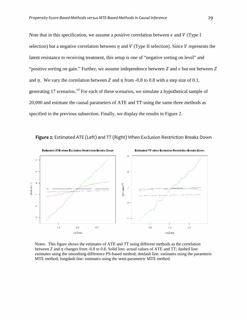
Figure 2: Estimated ATE (Left) and TT (Right) When Exclusion Restriction Breaks Down

Notes: This figure shows the estimates of ATE and TT using different methods as the correlation between 𝑍 and 𝜂 changes from -0.8 to 0.8. Solid line: actual values of ATE and TT; dashed line: estimates using the smoothing-difference PS-based method; dotdash line: estimates using the parametric MTE method; longdash line: estimates using the semi-parametric MTE method.


The left panel of Figure 2 shows the estimates of ATE, along with its actual values (solid

line). First of all, we can see that the MTE-based estimates of ATE are upwardly biased when

𝑐𝑜𝑟(𝑍, 𝜂) > 0 and downwardly biased when 𝑐𝑜𝑟(𝑍, 𝜂) < 0. In fact, the larger the correlation

between 𝑍 and 𝜂, the higher the estimates from the MTE-based methods, especially the semi-

parametric LIV estimates (longdash line). For example, when 𝑐𝑜𝑟(𝑍, 𝜂) is larger than 0.5, the

semi-parametric LIV estimates are greater than 6.0, twice as large as its actual value (3.0),

whereas the parametric MTE-based estimates (dotdash line) are upwardly biased by a smaller

magnitude, at about 4.0. In comparison, the PS-based estimates (dashed line) show a moderate

downward bias in this setup. As expected, the magnitude of bias for the PS-based estimates does

not depend on 𝑐𝑜𝑟(𝑍, 𝜂), because the PS-based estimates do not rely on 𝑍 as an IV for estimation.

The right panel of Figure 2 compares estimates of TT. Similar to the case of ATE, the

semi-parametric LIV approach yields estimates that are significantly upwardly biased when

𝑐𝑜𝑟(𝑍, 𝜂) > 0, and downwardly biased when 𝑐𝑜𝑟(𝑍, 𝜂) < 0. Nonetheless, the parametric MTE-

based estimates are almost equal to the true value of TT across the entire range of 𝑐𝑜𝑟(𝑍, 𝜂).

Finally, the PS-based estimates of TT show a significant underestimation. In fact, we may infer

this last result from an earlier discussion, as Table 2 indicates that TT is underestimated as long

as there is a negative sorting on level.

Overall, the above simulation reveals that, when there is a negative sorting on level (Type

I selection) and positive sorting on gain (Type II selection) due to unobservables, the MTE-based

methods, especially the semi-parametric LIV method, may severely over- or under-estimate ATE

and TT due to the use of an improper IV. As expected, the same causal parameters may be

underestimated by the PS-based method. As we will see in the next section, these results can

reasonably explain apparent discrepancies in results in an empirical example.


5. Empirical Example

To illustrate the three methods we discussed earlier, we applied them to the data used in

Carneiro, Heckman, and Vytlacil’s (2011) study of returns to college education using MTE. In

the subsections that follow, we (1) describe the data, (2) demonstrate the use of the smoothing-

difference PS-based method, (3) replicate Carneiro, Heckman, and Vytlacil’s (2011) results

using MTE, and (4) compare MTE-based and PS-based estimates of ATE and TT. In Appendix

A, we provide R codes that we used to generate the results presented in this section.

5.1. Data Description

Following Carneiro, Heckman, and Vytlacil (2011), we reanalyze a sample of white males

(N = 1747) who were 16-22 years old in 1979, drawn from the National Longitudinal Survey of

Youth 1979 (NLSY). Treatment is college attendance, measured by having attained any

postsecondary education by 1991. By this definition, the treated group consists of 865 subjects

and the control group consists of 882 subjects. The wage variable is measured as an average of

deflated (to 1983 constant dollars) non-missing hourly wages reported between 1989 and 1993.

Pretreatment covariates (𝑿) are urban residence at 14, AFQT score adjusted by years of

schooling, mother’s years of schooling, number of siblings, permanent local log earnings at 17

(county log earnings averaged between 1973 and 2000), permanent local unemployment rate at

age 17 (state unemployment rate averaged between 1973 and 2000) and cohort dummies.

Instrumental Variables (𝒁/𝑿) include (a) the presence of a four year college in the county of

residence at age 14, (b) local wage in the county of residence at age 17, (c) local unemployment

rate in the state of residence at age 17, and (d) average tuition in public 4-year colleges in the

county of residence at age 17. More detailed description of the dataset is provided in Carneiro,

Heckman, and Vytlacil (2011).


5.2. The Smoothing-Difference PS-Based Results

Below we show results from the smoothing-difference PS-based method. First of all, we estimate

the propensity score of attending college for each subject in the sample given 𝑿 using a probit

regression model. Table 3 presents the estimated propensity score model. We can see that the

likelihood of attending college is predicted positively by corrected AFQT score and negatively

by number of siblings and permanent local log earnings at age 17.

Table 3: Propensity Score Probit Model Predicting College Attendance

Predictors Coefficient

Urban Residence at 14 0.127 (0.084)

Corrected AFQT 0.667*** (0.045)

Corrected AFQT Squared 0.196*** (0.039)

Mother’s Years of Schooling -0.110 (0.089)

Mother’s Years of Schooling Squared 0.010** (0.004)

Number of Siblings -0.090†

(0.053)

Number of Siblings Squared 0.002 (0.006)

Permanent Local Log Earnings at 17 -43.9* (17.2)

Permanent Local Log Earnings at 17 Squared 2.15* (0.84)

Permanent State Unemployment Rate at 17 0.240 (0.369)

Permanent State Unemployment Rate at 17 Squared -0.018 (0.029)

Model χ2 684.4 (D.F.=18)

Notes: Numbers in parentheses are standard errors. †p<.1, *p<.05, **p<.01, ***p<.001


In the next step, we fit two separate nonparametric models regressing the log hourly wage

on the estimated propensity score, one for the treated group that went to college and one for the

untreated group that did not go to college. Here we use smoothing splines with 5 equivalent

degrees of freedom.15 Figure 3 displays the resulting curves, evaluated over the entire interval

(with a small portion being extrapolated). In the left panel, the dashed line and the dotdash line

show the expected log hourly wage respectively for those who went to college and for those who

did not.

Figure 3: The Smoothing-Difference PS-based Method for Estimating Returns to College

Notes: The left panel shows the expected annual wages respectively for those who attended college (dashed line) and for those who did not attend college (dotdash line). The right panel demonstrates the expected return to college for people with different propensity scores.

Two patterns emerge from this figure. First, for persons who attended college, the

expected wage increases steadily with the propensity score. That is, labor market outcomes differ

systematically among college goers, as those with a higher propensity to attend college earn

more than those with a lower propensity. Second, for persons who did not attend college,


expected wage shows a rapid increase at the lower end of propensity score but flattens out

thereafter. Hence, individuals who are very unlikely to go to college on the basis of their

observed covariates included in the propensity score are truly disadvantaged. If they do not go to

college, they earn much lower wages than their peers with a higher propensity to attend college

(e1.9 = 6.7 at 𝑝 ≈ 0, compared to e2.2 = 9.0 at 𝑝 ≈ 0.2). However, they also stand to gain a lot

from attending college (e2.2 = 9.0 at 𝑝 ≈ 0), although their wages are still substantially lower

than those of other college-goers with a higher propensity of attending college (e.g., e2.8 = 16.4

at 𝑝 ≈ 1.0).

We now turn to the right panel, which depicts estimated heterogeneous treatment effects

by propensity score.16 This curve is obtained directly by differencing the two functions in the left

panel. The non-monotonic pattern suggests that two groups of individuals exist who benefit most

from college: those most unlikely to go to college and those most likely to go to college.17 Thus,

college education seems to be more valuable for persons at either the low end or the high end of

the propensity score than for those in the middle. Therefore, from the data, we observe a mix of

positive selection and negative selection into college using the PS-based approach.

Next, we use the above curve to predict treatment effect 𝛿𝑖 for each individual 𝑖 in the

sample. We then average these δi′s over the entire sample to obtain ATE, and over those who

actually attended college to estimate TT. We will discuss these summary results in the next

subsection, comparing them to those produced by the MTE-based methods.

5.3. MTE-Based Results

We now give up the ignorability assumption and thus the propensity score approach. Instead, we

use the MTE-based methods, with covariates 𝑿 and instrumental variables (IVs) 𝒁/𝑿 specified

in Section 5.1. We first estimate two sets of marginal treatment effects, one from the parametric


model, and the other from the semi-parametric LIV method. Figure 4 plots these two sets

of MTE(𝒙,𝑢𝐷), both evaluated at mean values of 𝑿. Both the parametric and the semi-parametric

estimates of MTE show a declining trend with respect to 𝑢𝐷, i.e., the unobserved resistance to

attending college. These results show that individuals with higher returns to college are more

likely to go to college (in having lower 𝑢𝐷). Furthermore, the magnitude of the heterogeneity in

MTE is substantial: returns can vary from as high as 80%~100% (for low 𝑢𝐷 persons, who

would double their wages from attending college) to as low as -40% (for high 𝑢𝐷 persons, who

would lose from attending college).

Figure 4: Estimated Marginal Treatment Effects (averaged over 𝑿) from MTE-based Methods

Using weights provided by Heckman, Urzua, and Vytlacil (2006a), we construct standard

treatment parameters from the two sets of estimated MTE. Table 4 shows the final estimates of

ATE and TT from different methods, with bootstrapped standard errors. We observe that MTE-

based estimates of ATE and TT are less precise than those from the PS-based method. The lack

of precision for MTE-based estimates is expected since the IVs we use are relatively weak


compared to 𝑿 in determining treatment selection (see Section 4.2). More importantly, MTE-

based and PS-based results differ in magnitude. For ATE, the differences are not statistically

significant, although the semi-parametric LIV method seems to give a larger point estimate than

do the other two methods. For TT, the difference between MTE-based and PS-based results is

more substantial. Both the parametric and the semi-parametric MTE-based methods yield

significantly higher estimates of TT than the PS-based estimate. Specifically, we obtain the TT

estimate of college returns at 73.8% by the semi-parametric MTE method but only 27.8% by the

PS-based method.

Table 4: Estimates for Returns to College from NLSY data

Causal Parameters

MTE-Based Methods Smoothing-Difference PS-Based Method Parametric Semi-parametric

ATE 0.264

(0.159)

0.356

(0.174)

0.242

(0.067)

TT 0.567

(0.156)

0.736

(0.226)

0.278

(0.082)

Notes: Numbers in parentheses are bootstrapped standard errors with 250 repetitions.

Next, a natural question arises: why is there such a large discrepancy between PS-based

and MTE-based estimates, especially of TT? There is no firm answer to this question, but we can

offer some speculations. One possibility is that there may be an underestimation by the PS-based

method due to the breakdown of the ignorability assumption. In fact, the parametric MTE

approach provides the following estimates:

𝜎�𝜖𝑉 = 0.078, 𝜎�𝜂𝑉 = −0.239,


where 𝜎𝜖𝑉 and 𝜎𝜂𝑉 denote the covariances respectively between 𝜖 and 𝑉 and between 𝜂 and 𝑉.

Since 𝑉 represents a latent resistance to receiving treatment, these estimates imply a negative

Type I selection and a positive Type II selection due to unobservables. Note that our finding of a

negative Type I selection and a positive Type II selection accords well with Willis and Rosen’s

(1979) argument that college-goers would do more poorly if they did not go to college but

benefit more from college education than persons who do not go to college. If we can accept the

estimates as evidence for a negative Type I selection and a positive Type II selection, our earlier

discussion around Table 2 would suggest indeed a downward bias for the PS-based estimate of

TT.

Another possibility for the discrepancy in results in Table 4 is an overestimation by

MTE-based methods due to the violation of the exclusion restriction assumption. The numerical

simulation results in Section 4.3 suggest a potentially upward bias when there is a positive

correlation between IV and the treatment effect, i.e., 𝑐𝑜𝑟(𝑍, 𝜂) > 0 (for 𝛾 > 0). Unfortunately,

such a correlation is empirically unverifiable, since 𝜂 is an unobserved attribute that cannot be

individually recovered from the data. Hence, it is hard to adjudicate between these two

possibilities without further information.

6. Concluding Remarks

In this study, we have examined certain statistical properties of PS-based methods and MTE-

based methods through an exposition of identification issues, two simulation analyses, and an

empirical application. We found that the applicability of PS-based methods is not limited to

settings in which complete ignorability is satisfied. In fact, it is useful to decompose ignorability

into two components: (1) ignorability of Type I selection bias, or baseline difference between

treated and untreated units; (2) ignorability of Type II selection bias, or difference in treatment


effects between treated and untreated units. We have shown that as long as the ignorability of

Type I selection bias is satisfied, PS-based methods can still identify TT, even in the presence of

a heterogeneous treatment effect bias. Furthermore, when Type I selection bias cannot be

ignored, the bias for TT is in the same direction as the Type I selection bias.

By comparison, MTE-based methods are robust to different types of violation of the

ignorability assumption. However, they require strong instrumental variables that satisfy the

exclusion restriction assumption to achieve statistical efficiency. This is true for both the

parametric model and the semi-parametric method. If exclusion restriction is violated, MTE-

based methods can be subject to severe over- or under-estimation of treatment effects. In practice,

plausibility of the exclusion restriction assumption cannot be verified but can be evaluated based

on substantive knowledge about the research setting. In addition, we may assess the consequence

of a violation of the assumption through sensitivity analyses (for examples, see Angrist 1990;

Angrist, Imbens, and Rubin 1996).

This paper has also proposed a PS-based method based on first smoothing two

counterfactual outcomes, which we call the smoothing-difference method. Compared to

traditional matching and stratification methods, the smoothing-difference method has two

distinct advantages. On the one hand, it enables the researcher to examine the nonparametric

trends of counterfactual outcomes by treatment status across the spectrum of propensity score. In

our empirical example, we have shown the variations in wages by both the propensity score of

attending college and the status of college attendance. On the other hand, this method produces a

nonparametric pattern of treatment effect heterogeneity across individuals with different

propensity scores. Such an observed pattern of heterogeneity is of interest to social science

researchers, although its interpretation is still ambiguous, depending on the validity of

ignorability assumption (Brand and Xie 2010; Xie, Brand, and Jann 2012). For example, if the


ignorability assumption holds true, observed results reveal the pattern of heterogeneous treatment

effects. If one accepts only the ignorability of Type I selection bias, heterogeneous treatment

effects along the propensity score should be interpreted only for those who are actually treated. If

one does not embrace any form of ignorability, the observed pattern may reveal an underlying

selection process sorting out treated units from untreated units (Xie and Wu 2005).

References

Angrist, Joshua D. 1990. “Lifetime Earnings and the Vietnam Era Draft Lottery: Evidence from Social Security Administrative Records.” American Economic Review 80:313-335.

Angrist, Joshua D., Guido W. Imbens, and Donald B. Rubin. 1996. “Identification of Causal Effects Using Instrumental Variables.” Journal of the American Statistical Association 91(434): 444-455.

Angrist, Joshua D. and Alan B. Krueger. 1999. "Empirical Strategies in Labor Economics." Pp. 1277-1366 in Handbook of Labor Economics, Vol. 3A, edited by O. Ashenfelter and D. Card. Amsterdam: Elsevier.

Ansari, Asim and Jedidi Kamel. 2000. “Bayesian Factor Analysis for Multilevel Binary Observations.” Psychometrika 65:475-496.

Bauer, Daniel J. and Patrick J. Curran. 2003. “Distributional Assumptions of Growth Mixture Models: Implications for Overextraction of Latent Trajectory Classes.” Psychological Methods 8:338-363.

Bjorklund, Anders and Robert Moffitt. 1987. “The Estimation of Wage Gains and Welfare Gains in Self-Selection Models.” The Review of Economics and Statistics 69: 42-49.

Blundell, Richard, Lorraine Dearden, and Barbara Sianesi. 2005. “Evaluating the Effect of Education on Earnings: Models, Methods, and Results from the National Child Development Survey.” Journal of the Royal Statistical Society: Series A 168: 473-512.

Brand, Jennie E. and Yu Xie. 2010. “Who Benefits Most from College? Evidence for Negative Selection in Heterogeneous Economic Returns to Higher Education.” American Sociological Review 75(2):273-302.

Carneiro, Pedro, James Heckman, and Edward Vytlacil. 2011. “Estimating Marginal Returns to Education.” Forthcoming in American Economic Review.

Cornfield, Jerome, William Haenszel, E. Cuyler Hammond, Abraham M. Lilienfeld, Michael B. Shimkin, and Ernst L. Wynder. 1959. “Smoking and Lung Cancer: Recent Evidence and a Discussion of Some Questions.” Journal of the National Cancer Institute 22:173-203.

DiPrete, Thomas and Markus Gangl. 2004. "Assessing Bias in the Estimation of Causal Effects: Rosenbaum Bounds on Matching Estimators and Instrumental Variables Estimation with Imperfect Instruments." Sociological Methodology 34:271-310.

Greenland Sander, and Charles Poole. 1988. “Invariants and Noninvariants in the Concept of Interdependent Effects.” Scandinavian Journal of Work, Environment & Health 14:125-129.


Harding, David J. 2003. “Counterfactual Models of Neighborhood Effects: The Effect of Neighborhood Poverty on High School Dropout and Teenage Pregnancy.” American Journal of Sociology 109(3):676-719.

Hastie, Trevor, Robert Tibshirani and Jerome Friedman. 2008. The Elements of Statistical Learning: Data Mining, Inference and Prediction. Springer.

Heckman, James J. 1979. “Sample Selection Bias as a Specification Error.” Econometrica 47: 153-161.

——. 2001. “Micro Data, Heterogeneity, and the Evaluation of Public Policy: Nobel Lecture.” Journal of Political Economy 109:673-748.

——. 2005. “The Scientific Model of Causality.” Sociological Methodology 35:1-98.

Heckman, James J. and Salvador Navarro-Lozano. 2004. “Using Matching, Instrumental Variables, and Control Functions to Estimate Economic Choice Models.” The Review of Economics and Statistics 86:30-57.

Heckman, James J. and Richard Robb. 1985. “Alternative Methods for Evaluating the Impact of Interventions.” Pp.156-245 in Longitudinal Analysis of Labor Market Data, edited by James Heckman and Burton Singer. Cambridge: Cambridge University Press.

Heckman, James J., Sergio Urzua, and Edward Vytlacil. 2006a. “Understanding Instrumental Variables in Models with Essential Heterogeneity.” The Review of Economics and Statistics 88:389-432.

——. 2006b. “Estimation of Treatment Effects under Essential Heterogeneity.” Retrieved October 12, 2010 (http://jenni.uchicago.edu/underiv/documentation_2006_03_20.pdf).

Heckman, James J. and Edward J. Vytlacil. 1999. “Local Instrumental Variables and Latent Variable Models for Identifying and Bounding Treatment Effects.” Proceedings of the National Academy of Sciences of the United States of America 96:4730-4734.

——. 2001. “Local Instrumental Variables.” Pp. ---- in Nonlinear Statistical Modeling: Proceedings of the Thirteenth International Symposium in Economic Theory and Econometrics: Essays in Honor of Takeshi Amemiya, edited by Cheng Hsiao, Kimio Morimune, and James, L. Powel. New York: Cambridge University Press.

——. 2005. “Structural Equations, Treatment Effects, and Econometric Policy Evaluation.” Econometrica 73:669-738.

Holland, Paul W. 1986. “Statistics and Causal Inference.” Journal of American Statistical Association 81:945-960.

Lubke, Gitta H. and Bengt Muthen. 2005. “Investigating Population Heterogeneity with Factor Mixture Models.” Psychological Methods 10:21-39.

Manski, Charles. 1995. Identification Problems in the Social Sciences. Boston, MA: Harvard University Press.

——. 2007. Identification for Prediction and Decision. Cambridge: Harvard University Press.

Moffitt, Robert. 1996. “Identification of Causal Effects Using Instrumental Variables: Comment.” Journal of the American Statistical Association 91:462-465.

Moffitt, Robert. 2008. “Estimating Marginal Treatment Effects in Heterogeneous Populations.” Annuals of Economics and Statistics 91/92:239-261.

Morgan, Stephen and Christopher Winship. 2007. Counterfactuals and Causal Inference: Methods and Principles for Social Research. Cambridge, UK: Cambridge University Press.

http://jenni.uchicago.edu/underiv/documentation_2006_03_20.pdf


Pearl, Judea. 2009. Causality: Models, Reasoning, and Inference. Second Edition. NewYork: Cambridge University Press.

Puhani, Patrick. 2000. “The Heckman Correction for Sample Selection and Its Critique.” Journal of Economic Surveys 14:53-68.

Rosenbaum, Paul R. 2002. Observational Studies. New York: Springer.

Rosenbaum, Paul R. and Donald B. Rubin. 1983. “The Central Role of the Propensity Score in Observational Studies for Causal Effects.” Biometrika 70:41–55.

——. 1984. “Reducing Bias in Observational Studies Using Subclassification on the Propensity Score.” Journal of the American Statistical Association 79:516-524.

Rothman, Kenneth J. and Sander Greenland, eds. 1998. Modern Epidemiology, 2nd Edition. Lippincott-Raven Publishers: Philadelphia, PA.

Rubin, Donald B. 1974. “Estimating Causal Effects of Treatments in Randomized and Nonrandomized Studies.” Journal of Educational Psychology 66: 688-701.

——. 1986. “What Ifs Have Causal Answers?” Journal of American Statistical Association 81:961-962.

——. 1997. “Estimating Causal Effects from Large Data Sets Using Propensity Scores.” Annals of Internal Medicine 5(127) (8 Pt 2):757-763.

Shadish, William R., M.H. Clark and Peter M. Steiner. 2008. “Can Nonrandomized Experiments Yield Accurate Answers? A Randomized Experiment Comparing Random and Nonrandom Assignments.” Journal of American Statistical Association 103(484):1334-1344.

Sobel, Michael E. 2000. “Causal Inference in the Social Science.” Journal of the American Statistical Association 95: 647-651.

Tsai, Shu-Ling, and Yu Xie. 2011. “Heterogeneity in Returns to College Education: Selection Bias in Contemporary Taiwan.” Social Science Research 40:796-810.

Willis, Robert J. and Sherwin Rosen. 1979. “Education and Self-Selection.” Journal of Political Economy 87:S7-S36.

Winship, Christopher and Stephen L. Morgan. 1999. “The Estimation of Causal Effects from Observational Data.” Annual Review of Sociology 25:659-707.

Winship, Christopher and Michael Sobel. 2004. “Causal Inference in Sociological Studies.” Pp. 481-503 in Handbook of Data Analysis, edited by Melissa Hardy and Alan Bryman. Sage Publications Ltd.

Woodridge, Jeffery M. 2001. Econometric Analysis of Cross Section and Panel Data, 1st Edition. Cambridge: The MIT Press.

Xie, Yu. 2000. “Assessment of the Long-Term Benefits of Head Start.” Pp.139-167 in Into Adulthood: A Study of the Effects of Head Start, edited by Sherri Oden, Lawrence J. Schweinhart, and David P. Weikart. Ypsilanti, MI: High/Scope Press.

——. 2007. “Otis Dudley Duncan’s Legacy: the Demographic Approach to Quantitative Reasoning in Social Science.” Research in Social Stratification and Mobility.

Xie, Yu, Jennie Brand and Ben Jann. 2012. “Estimating Heterogeneous Treatment Effects with Observational Data.” Forthcoming in Sociological Methodology.

Xie, Yu and Xiaogang Wu. 2005. “Market Premium, Social Process, and Statisticism.” American Sociological Review 70:865-870.


Appendix A: R Implementation of Different Methods for the NLSY Data This appendix provides the R codes that were used to estimate returns to college for the NLSY data. The dataset we use is available upon request. The Smoothing-Difference PS-based Method:

library(Hmisc) library(survival) library(splines) library(KernSmooth) library(stats) #Read Data# nlsy=read.table("nlsyfinal.csv",sep=",",header=T) #Propensity Score Model# prps=glm(state~urban14+numsibs+I(numsibs^2)+mhgc+I(mhgc^2)+cafqt+I(cafqt^2)+d57+d58+d59+d60+d61+d62+d63+lavlocwage17+I(lavlocwage17^2)+avurate+I(avurate^2),family=binomial(link="probit"),data=nlsy) #Extract Fitted Propensity Scores# ps=prps$fitted nlsy=cbind(nlsy,ps) attach(nlsy) # PS-based Smoothing Splines# nlsy1=nlsy[state==1,] nlsy0=nlsy[state==0,] ps.ss1=smooth.spline(nlsy1$ps,nlsy1$wage,df=5) ps.ss0=smooth.spline(nlsy0$ps,nlsy0$wage,df=5) pred.ss1=predict(ps.ss1,ps)$y pred.ss0=predict(ps.ss0,ps)$y TE.pred.ss=pred.ss1-pred.ss0 #Estimating ATE and TT# ATE.ss=mean(TE.pred.ss) TT.ss=sum(TE.pred.ss*state)/sum(state) #Plot of Heterogeneous Treatment Effect along the Propensity Score# x=seq(0.005,0.995,0.01) y1=predict(ps.ss1,x)$y y0=predict(ps.ss0,x)$y plot(x,y1-y0,type="l",xlab="Propensity Score",ylab="Treatment Effect of College")


The Parametric and Semi-parametric MTE-Based Methods:

library(Hmisc) library(survival) library(splines) library(KernSmooth) library(stats) library(sampleSelection) nlsy=read.table("nlsyfinal.csv",sep=",",header=T) attach(nlsy) N=dim(nlsy)[1] #Propensity Score Model for MTE-based Methods# prps=glm(state~urban14+numsibs+I(numsibs^2)+mhgc+I(mhgc^2)+cafqt+I(cafqt^2)+d57+d58+d59+d60+d61+d62+d63+lavlocwage17+I(lavlocwage17^2)+avurate+I(avurate^2)+pub4+pub4*cafqt+pub4*mhgc+pub4*numsibs+lwage5_17+lwage5_17*cafqt+lwage5_17*mhgc+lwage5_17*numsibs+lurate_17+lurate_17*cafqt+lurate_17*mhgc+lurate_17*numsibs+tuit4c+tuit4c*cafqt+tuit4c*mhgc+tuit4c*numsibs,family=binomial(link="probit"),data=nlsy) #Extract Fitted Propensity Scores# ps=prps$fitted # Estimation of TT&ATE Weights # ud=array(0,c(1,100)) for (i in seq(1,100)){ud[i]=-0.005+0.01*i} nume=array(0,c(N,100)) deno=array(0,c(N,1)) wate=array(1/100,c(N,100)) wtt=array(0,c(N,100)) for (i in seq(1,100)){ wtt.S=(ps>ud[i]) wtt.glm=glm(wtt.S~exp+d57+d58+d59+d60+d61+d62+d63+expsq+urban14+numsibs+I(numsib^2)+cafqt+I(cafqt^2)+mhgc+I(mhgc^2)+lavlocwage17+I(lavlocwage17^2)+avurate+I(avurate^2)+lwage5+lurate,family=binomial(link="probit"))nume[,i]=wtt.glm$fitted} for (i in seq(1,N)){deno[i]=sum(nume[i,])for (j in seq(1,100)){wtt[i,j]=nume[i,j]/deno[i]}} #PARAMETRIC MTE-BASED METHOD# #Heckman Selection Model# heckit=selection(state~urban14+numsibs+I(numsibs^2)+mhgc+I(mhgc^2)+cafqt+I(cafqt^2)+d57+d58+d59+d60+d61+d62+d63+lavlocwage17+I(lavlocwage17^2)+avurate+I(avurate^2)+pub4+pub4*cafqt+pub4*mhgc+pub4*numsibs+lwage5_17+lwage5_17*cafqt+lwage5_17*mhgc+lwage5_17*numsibs+lurate_17+lurate_17*cafqt+lurate_17*mhgc+lurate_17*numsibs+tuit4c+tuit4c*cafqt+tuit4c*mhgc+tuit4c*numsibs,list(wage~exp+d57+d58+d59+d60+d61+d62+d63+expsq+urban14+numsibs+I(numsibs^2)+cafqt+I(cafqt^2)+mhgc+I(mhgc^2)+lavlocwage17+I(lavlocwage17^2)+avurate


+I(avurate^2)+lwage5+lurate,wage~exp+d57+d58+d59+d60+d61+d62+d63+expsq+urban14+numsibs+I(numsibs^2)+cafqt+I(cafqt^2)+mhgc+I(mhgc^2)+lavlocwage17+I(lavlocwage17^2)+avurate+I(avurate^2)+lwage5+lurate),nlsy) #Create a Data-frame for X# X=data.frame(1,exp,d57,d58,d59,d60,d61,d62,d63,expsq,urban14,numsibs,numsibs^2,cafqt,cafqt^2,mhgc,mhgc^2,lavlocwage17,lavlocwage17^2,avurate,avurate^2,lwage5,lurate) #Estimated Coefficients of X in MTE, that is, 𝛽1 − 𝛽0# X.coef=heckit$estimate[61:83]-heckit$estimate[36:58] #Estimated Coefficient of Φ−1(𝑢𝐷) in MTE, that is, 𝜎𝜂𝑉# ud.coef=-heckit$estimate[85]*heckit$estimate[84]+heckit$estimate[59]*heckit$estimate[60] #Parametric Estimation of MTE # MTE.par=array(0,c(N,100)) MTE.par.x=as.matrix(X) %*% matrix(X.coef) for (i in seq(1,N)){for (j in seq(1,100)){MTE.par[i,j]=MTE.par.x[i]+ud.coef*qnorm(ud[j])}} #Plot of Parametric MTE# plot(seq(0.005,0.995,0.01),apply(MTE.par,2,mean),type="l",xlab="Ud",ylab="MTE",main="Parametric Estimates of MTE") #Parametric Estimation of ATE and TT# ATE.par.x=apply(MTE.par*wate,1,sum) TT.par.x=apply(MTE.par*wtt,1,sum) ATE.par=mean(ATE.par.x) TT.par=sum(TT.par.x*state)/sum(state) #SEMI-PARAMETRIC MTE-BASED METHOD# #Semi-parametric Estimation of MTE: Step 1# exp.res=loess(exp~ps,degree=1)$res expsq.res=loess(expsq~ps,degree=1)$res lwage5.res=loess(lwage5~ps,degree=1)$res lurate.res=loess(lurate~ps,degree=1)$res lavlocwage17.res=loess(lavlocwage17~ps,degree=1)$res lavlocwage17sq.res=loess(lavlocwage17^2~ps,degree=1)$res avurate.res=loess(avurate~ps,degree=1)$res avuratesq.res=loess(avurate^2~ps,degree=1)$res cafqt.res=loess(cafqt~ps,degree=1)$res cafqtsq.res=loess(cafqt^2~ps,degree=1)$res mhgc.res=loess(mhgc~ps,degree=1)$res mhgcsq.res=loess(mhgc^2~ps,degree=1)$res numsibs.res=loess(numsibs~ps,degree=1)$res


numsibssq.res=loess(numsibs^2~ps,degree=1)$res d57.res=loess(d57~ps,degree=1)$res d58.res=loess(d58~ps,degree=1)$res d59.res=loess(d59~ps,degree=1)$res d60.res=loess(d60~ps,degree=1)$res d61.res=loess(d61~ps,degree=1)$res d62.res=loess(d62~ps,degree=1)$res d63.res=loess(d63~ps,degree=1)$res urban14.res=loess(urban14~ps,degree=1)$res psexp.res=loess(ps*exp~ps,degree=1)$res psexpsq.res=loess(ps*expsq~ps,degree=1)$res pslwage5.res=loess(ps*lwage5~ps,degree=1)$res pslurate.res=loess(ps*lurate~ps,degree=1)$res pslavlocwage17.res=loess(ps*lavlocwage17~ps,degree=1)$res pslavlocwage17sq.res=loess(ps*lavlocwage17^2~ps,degree=1)$res psavurate.res=loess(ps*avurate~ps,degree=1)$res psavuratesq.res=loess(ps*avurate^2~ps,degree=1)$res pscafqt.res=loess(ps*cafqt~ps,degree=1)$res pscafqtsq.res=loess(ps*cafqt^2~ps,degree=1)$res psmhgc.res=loess(ps*mhgc~ps,degree=1)$res psmhgcsq.res=loess(ps*mhgc^2~ps,degree=1)$res psnumsibs.res=loess(ps*numsibs~ps,degree=1)$res psnumsibssq.res=loess(ps*numsibs^2~ps,degree=1)$res psd57.res=loess(ps*d57~ps,degree=1)$res psd58.res=loess(ps*d58~ps,degree=1)$res psd59.res=loess(ps*d59~ps,degree=1)$res psd60.res=loess(ps*d60~ps,degree=1)$res psd61.res=loess(ps*d61~ps,degree=1)$res psd62.res=loess(ps*d62~ps,degree=1)$res psd63.res=loess(ps*d63~ps,degree=1)$res psurban14.res=loess(ps*urban14~ps,degree=1)$res wage.res=loess(wage~ps,degree=1)$res #Semi-parametric Estimation of MTE: Step 2# double.res=lm(wage.res~0+exp.res+expsq.res+lwage5.res+lurate.res+lavlocwage17.res+lavlocwage17sq.res+avurate.res+avuratesq.res+cafqt.res+cafqtsq.res+mhgc.res+mhgcsq.res+numsibs.res+numsibssq.res+d57.res+d58.res+d59.res+d60.res+d61.res+d62.res+d63.res+urban14.res+psexp.res+psexpsq.res+pslwage5.res+pslurate.res+pslavlocwage17.res+pslavlocwage17sq.res+psavurate.res+psavuratesq.res+pscafqt.res+pscafqtsq.res+psmhgc.res+psmhgcsq.res+psnumsibs.res+psnumsibssq.res+psd57.res+psd58.res+psd59.res+psd60.res+psd61.res+psd62.res+psd63.res+psurban14.res) temp.X=data.frame(exp,expsq,lwage5,lurate,lavlocwage17,lavlocwage17^2,avurate,avurate^2,cafqt,cafqt^2,mhgc,mhgc^2,numsibs,numsibs^2,d57,d58,d59,d60,d61,d62,d63,urban14,ps*exp,ps*expsq,ps*lwage5,ps*lurate,ps*lavlocwage17,ps*lavlocwage17^2,ps*avurate,ps*avurate^2,ps*cafqt,ps*cafqt^2,ps*mhgc,ps*mhgc^2,ps*numsibs,ps*numsibs^2,ps*d57,ps*d58,ps*d59,ps*d60,ps*d61,ps*d62,ps*d63,ps*urban14)


wage.latent=wage-as.matrix(temp.X) %*% matrix(double.res$coef) #Semi-parametric Estimation of MTE: Step 3# MTE.semi.ud=locpoly(ps,wage.latent,drv=1L,bandwidth=0.32,gridsize=100L,range.x=c(0.005,0.995)) #Semi-parametric Estimation of MTE: Step 4# MTE.semi=array(0,c(N,100)) MTE.semi.x=as.matrix(temp.X[,1:22]) %*% matrix(double.res$coef[23:44]) for (i in seq(1,N)){for (j in seq(1,100)){MTE.semi[i,j]=MTE.semi.x[i]+MTE.semi.ud$y[j]}} #Plot of Semi-parametric MTE# plot(seq(0.005,0.995,0.01),apply(MTE.semi,2,mean),type="l",xlab="Ud",ylab="MTE",main="Semi-parametric Estimates of MTE") # Semiparametric Estimation of ATE and TT# ATE.semi.x=apply(MTE.semi*wate,1,sum) TT.semi.x=apply(MTE.semi*wtt,1,sum) ATE.semi=mean(ATE.semi.x) TT.semi=sum(TT.semi.x*state)/sum(state)


Notes

1 The exact meaning of the strength of an instrumental variable will be defined in Section 4. 2 An implicit condition for defining causal effects within the counterfactual framework is the stable-

unit-treatment-value assumption (SUTVA), which requires that the value of 𝛿𝑖 does not depend on what mechanism is used to assign the treatment to subject 𝑖, or what treatments the other subjects receive (Rubin 1986).

3 There is a guarantee of comparability of the treated group and the control group in an experiment. In this paper, we restrict our attention to observational studies.

4 These two equations constitute a necessary but not sufficient condition for the ignorability assumption (5). In the literature, they are usually called the “weak ignorability assumption” or “conditional mean independence.” See Woodridge (2001).

5 Alternative nonparametric regression techniques, such as kernel methods and local polynomial regression, could also be applied here.

6 Xie, Brand and Jann (2012) also provide a comparison between this method and other PS-based methods.

7 In this case, Type I selection bias due to unobservables could be reduced by other methods such as the conventional IV approach, the fixed-effect model, and regression discontinuity designs (after conditioning on the propensity score).

8 The linearity assumption is convenient but not necessary. We can generally assume 𝑌0 = 𝜇0(𝑿) +𝜖 and 𝑌1 = 𝜇1(𝑿) + 𝜖 + 𝜂 for any given functions µ0(𝑿) and µ1(𝑿).

9 Weights for different parameters of interest are given in Heckman, Urzua, and Vytlacil (2006a). 10 For specific issues on the implementation of this semi-parametric MTE method, see Heckman,

Urzua, and Vytlacil (2006b). 11 An illustrative simulation study for the MTE-based approach is given in Heckman, Urzua, and

Vytlacil (2006b). However, the authors considered only the situation where variables in 𝒁 and variables in 𝑿 are mutually exclusive and independent, i.e., the treatment selection equation is purely determined by instrumental variables, which is rather unrealistic.

12 For the parametric model, a detailed discussion on the asymptotic variance of the maximum likelihood estimator could be found in Heckman (1979) and Puhani (2000).

13 For a discussion of whether to include IV in estimating the propensity score, see Pearl (2009). 14 For the covariance matrix of (𝜖, 𝜂,𝑉,𝑍) to be positive definite, the correlation between 𝜂 and 𝑍

cannot exceed 0.8. 15 Alternative choices of the smoothing parameter do not substantially alter our results. 16 For a discussion of why such heterogeneity is of special interest, see Xie, Brand, and Jann (2012). 17 The second part of this finding, i.e., a larger return at the very high level of the propensity score, is

inconsistent with Brand and Xie’s (2010) main conclusion. Future research is needed to explain this inconsistency.

Propensity-Score-Based Methods versus MTE-Based … · Propensity-Score-Based Methods versus MTE...

Documents

Transcript of Propensity-Score-Based Methods versus MTE-Based … · Propensity-Score-Based Methods versus MTE...