Applied Intelligencehttps://doi.org/10.1007/s10489-020-01837-7

Proof searching and prediction in HOL4 with evolutionary/heuristicand deep learning techniques

M. Saqib Nawaz1 ·M. Zohaib Nawaz2,3 ·Osman Hasan2 · Philippe Fournier-Viger1 ·Meng Sun4

© Springer Science+Business Media, LLC, part of Springer Nature 2020

AbstractInteractive theorem provers (ITPs), also known as proof assistants, allow human users to write and verify formal proofs.The proof development process in ITPs can be a cumbersome and time-consuming activity due to manual user interactions.This makes proof guidance and proof automation the two most desired features for ITPs. In this paper, we first providetwo evolutionary and heuristic-based proof searching approaches for the HOL4 proof assistant, where a genetic algorithm(GA) and simulated annealing (SA) is used to search and optimize the proofs in different HOL theories. In both approaches,random proof sequences are first generated from a population of frequently occurring HOL4 proof steps that are discoveredwith sequential pattern mining. Generated proof sequences are then evolved using GA operators (crossover and mutation)and by applying the annealing process of SA till their fitness match the fitness of the target proof sequences. Experimentswere done to compare the performance of SA with that of GA. Results have shown that the two proof searching approachescan be used to efficiently evolve the random sequences to obtain the target sequences. However, these approaches lack theability to learn the proof process, that is important for the prediction of new proof sequences. For this purpose, we proposeto use a deep learning technique known as long short-term memory (LSTM). LSTM is trained on various HOL4 theoriesfor proof learning and prediction. Experimental results suggest that combining evolutionary/heuristic and deep learningtechniques with proof assistants can greatly facilitate proof finding/optimization and proof prediction.

Keywords HOL4 · Genetic algorithm · Simulated Annealing · LSTM · Proof searching · Proof learning · Fitness

1 Introduction

Theorem proving is a popular formal verification method thatis used for the analysis of both hardware and software systems.In theorem proving, the system that needs to be analyzed isfirst modeled and specified in an appropriate mathematicallogic. Important/critical properties of the system are then ver-ified using theorem provers [1] based on deductive reason-ing. The initial objective of developing theorem provers wasto enable mathematicians to prove theorems using com-puter programs within a sound environment. However, thesemechanical tools have evolved in last two decades and nowplay a critical part in the modeling and reasoning about

M. Saqib Nawaz and M. Zohaib Nawaz equally contributedto the paper.

� Philippe Fournier-Vigerphilfv8@yahoo.com

Extended author information available on the last page of the article.

complex and large-scale systems, particularly safety-criticalsystems. Today, theorem provers are used in verificationprojects that range from compilers, operating systems andhardware components to prove the correctness of largemathematical proofs such as the Kepler conjecture and theFeit-Thomson Theorem [2].

There are two main categories of theorem provers: Auto-mated theorem provers (ATPs) and interactive theoremprovers (ITPs). ATPs are generally based on propositionaland first-order logic (FOL) and involve the development ofcomputer programs that has the ability to automatically per-form logical reasoning. However, FOL is less expressivein nature and cannot be used to define complex problems.Moreover, no ATPs can be scaled to the large mathematicallibraries due to the problem of search space (combinatorial)explosion. On the other hand, ITPs are based on higher-order logic (HOL), which allows quantification over predi-cates and functions and thus offers rich logical formalismssuch as (co)inductive and dependent types as well as recur-sive functions. This expressive power leads to the unde-cidability problem, i.e., the reasoning process cannot be

M. Saqib Nawaz et al.

automated in HOL and requires some sort of human guid-ance during the process of proof searching and develop-ment. That is why ITPs are also known as proof assistants.Some well-known proof assistants are HOL4 [3], Coq [4]and PVS [5].

Most studies and efforts on designing proof assistantsaim at making the proof checking process easier to userswhile ensuring proof correctness, and at providing an effi-cient proof development environment for users. The proofdevelopment process in ATPs is generally automatic.Whereas, ITPs follow the user driven proof developmentprocess. The user guides the proof process by providing theproof goal and by applying proof commands and tactics toprove the goal. Generally, an ITP user is involved in lots ofrepetitive work while verifying a nontrivial theorem (proofgoal), and thus the overall process is quite laborious andtedious as well as time consuming. For example, a list of 100mechanically verified mathematical theorems is available at[6]. The writing and verification process for many of thesetheorems required several months or even years (approx-imately 20 years for the Kepler conjecture proof in HOLLight [7] and twice as much for the Feit-Thompson theoremin Coq [8]) and the complete proofs contain thousands oflow-level inference steps. Another example is the CompCert[9] compiler, that took 6 person-years and approximately100,000 lines of Coq to write and verify.

The formal proof of a goal in ITPs, such as HOL4, mainlydepends on the specifications available in a theory or a set oftheories along with different combinations of proof com-mands, inference rules, intermediate states and tactics. Becausea theory in ITPs often contains many definitions and theo-rems [10–12], it is quite inefficient to apply a brute forceor pure random search based approach for proof searching.This makes proof guidance and proof automation along withproof searching an extremely desirable feature for ITPs.

However, proof scripts for theories in ITPs can be com-bined together to develop a more complex computer-under-standable corpora. With the evolution in information andcommunication technologies (ICT) in the last decade, it isnow possible to use deep mining and learning techniqueson such corpora for guiding the proof search process, forproof automation and for the development of proof tac-tics/strategies, as indicated in the works done in [2, 13–17].

In previous work, we proposed an evolutionary approach[18] for proof searching and optimization in HOL4. Thebasic idea is to use a Genetic Algorithm (GA) for proofsearching where an initial population (a set of potentialsolutions) is first created from frequent HOL proof stepsthat are discovered using a sequential pattern mining(SPM)-based proof guidance approach [17]. Random proofsequences from the population are then generated byapplying two GA operators (crossover and mutation). Both

operators randomly evolve the random proof sequences byshuffling and changing the proof steps at particular points.This process of crossover and mutation continues till thefitness of random proof sequences matches the fitness oforiginal (target) proofs for the considered theorems/lemmas.Various crossover and mutation operators were used tocompare their effect on the performance of GAs in proofsearching. The approach was successfully used on sixtheories taken from the HOL4 library. This proof searchingapproach [18] is quite efficient in evolving random proofsefficiently. However, alternative proof searching approachescould be developed. Moreover, the approach is unable tolearn the previously proved facts and to predict the proofsfor new unproved theorems/lemmas (conjectures).

This paper addresses these issues by comparing evo-lutionary and heuristic-based proof searching approachesfor HOL4 and proposing a deep neural networks basedapproach to learn the proof process and to predict proofs.The tasks of proof learning and prediction in theoremprovers are mainly related to the task of premise selection,where relevant statements (formulas) that are important anduseful to prove a conjecture are selected. This means that fora given dataset of already proved facts and a user providedconjecture, the problem of premise selection is to determinethose facts that will lead to a successful proof of the con-jecture. The proof searching approaches cannot be used tofind a sequence of deductions that will lead from presumedfacts to the given conjecture. The reason for this is that thestate-space of the proof search is combinatorial in nature,where the search can quickly explode, despite the fact thatsome facts are often relevant for proving a given conjecture.On the other hand, the applicability of deep neural networksin embedding the semantic meaning and logical relation-ships into geometric spaces suggest their possible usage toguide the combinatorial search for the proofs in theoremprovers. This paper extends the work published in [18] withthe following contributions:

1. A heuristic-based approach is provided, where simu-lated annealing (SA) is used for proof searching andoptimization. The performance of SA is compared withthat of GA [18] for various parameter values. It is foundthat SA outperforms GA for proof finding and opti-mization. Moreover, we elaborate on how pure randomsearching and a brute force approach are not suitable forthis task.

2. LSTM is used on HOL4 theories for learning andpredicting proof sequences. The basic idea is to firstconvert the proofs in HOL4 libraries into a suitableformat (vectors (tensors)) so that LSTM can processthem. LSTM then learns from the proofs and predictsnew proof sequences.

Proof Searching and Prediction in HOL4

3. For experimental evaluation, we have selected 14theories from the HOL4 library. All three approachesare used on these theories and the detailed results arepresented in this paper.

The rest of this paper is organized as follows: Section 2discusses the related work. Section 3 briefly discussesthe HOL4 theorem prover, GAs, SA and recurrent neuralnetworks (RNNs). Section 4 presents the proposed proofsearching approaches, where GA and SA are used to findand optimize random HOL4 proofs. Evaluation of theproposed approaches on different theories of the HOL4library is presented in Section 5. Section 6 presents theproof learning approach that is based on LSTM along withobtained results. Finally, Section 7 concludes the paperwhile highlighting some future directions.

2 Related work

In this section, we present the related work on theintegration of evolutionary and heuristic algorithms in ITPs,followed by the use of deep learning techniques for the taskof proof guidance and premise selection in theorem provers.

2.1 Evolutionary algorithms in ITPs

A GA was used in [19, 20] with the Coq proof assistantto automatically find formal proofs of theorems. However,the approach can only be used to successfully find theproofs of very small theorems that contain less numberof proof steps. Whereas, for large and complex theoremsthat require induction and depend on the proofs of otherlemmas, interaction between the proof assistant and the useris still required. Similarly, genetic programming [21] and apairwise combination (that focuses only on crossover basedapproach) were used in [22] on patterns (simple tactics)discovered in Isabelle proofs to evolve them into compoundtactics. However, Isabelle’s proofs have to be representedusing a linearized tree structure where the proofs aredivided into separate sequences and weights are assignedto these sequences. Linearization of proofs tree leads to theloss of important connections (information) among variousbranches. Because of this, interesting patterns and tacticsmay be lost in the evolution process. In this work, thedataset for the proof sequences contains all the necessaryinformation that is required for the discovery of frequentproof steps, through which initial population for the GAand SA is generated. Moreover, in both approaches, nohuman guidance is required during the evolution process forrandom proof sequences.

2.2 Deep learning in theorem provers

The task of premise selection with machine learning wasfirst investigated in [23] in the ATP Vampire, where acorpus for Mizar proofs was constructed for training twoclassifiers with bag-of-word features that represent theterms occurrences in a vocabulary. Deep learning techniques(recurrent and convolutional neural networks) were firstused in [15] for premise selection on the Mizar proofs(represented as FOL formulas) corpus. Experiments weredone in the ATP E. Similarly, deep networks have beenused in [24] for internal guidance in E. A hybrid (two-phase) approach was used on the Mizar proofs for theselection of clauses during proof search. However, the treerepresentation of proofs in first-order formulas was notinvariant to variable renaming and was unable to capture thebinding of variables by quantifiers. For large datasets, theHolStep dataset was introduced in [2], which consists of 2Mstatements and 10K conjectures. A deep learning approachwas provided in [25], where formulas were representedas graphs that were then embedded into a vector space.Finally, formulas were classified by relevance. Experimentswere performed on the HolStep dataset and obtained resultsshowed better performance than sequence-based models.

GRU networks were used in [26] for guiding the proofsearch of a tableau style proof process in MetaMath. How-ever, both approaches [25, 26] are tree-based approaches.Premise selection techniques were developed in [16] for theCoq system, where various machine learning methods wereused and compared for learning the dependencies in proofstaken from the CoRN repository. Premise selection basedon machine learning and automated reasoning for HOL4 isprovided in [27] by adapting HOL(y)Hammer [28]. Tactic-toe, a learning approach based on Monte Carlo tree searchalgorithm, was developed in [14] for HOL4 to automatetheorems proofs.

Recently, RNNs and LSTMs were used in [29] to predictand suggest the tactics for the (semi)-automation of theproof process in one Coq theory. Compared with thementioned approaches, our deep learning method does notrely on carefully engineered features and has the abilityto learn from the textual representation of HOL4 proofs,without the need of converting the proofs to FOL formulasor representing them with graphs.

3 Preliminaries

A brief introduction to the HOL4 proof assistant, GA,SA and RNN is provided in this section to facilitate theunderstanding of the rest of the paper.

M. Saqib Nawaz et al.

3.1 HOL4

HOL4 [3] is an ITP that utilizes the simple type theory alongwith Hindley-Milner polymorphism for the implementationof HOL. The logic in HOL4 is represented with thestrongly-typed functional programming language metalanguage (ML). An ML abstract data type is used to definetheorems and the only way to interact with the theoremprover is by executing ML procedures that operate on valuesof these data types. A theory in HOL4 is a collection ofdefinitions, axioms, types, constants theorems and proofs, aswell as tactics. The theories in HOL4 are stored as ML files.Users can reload a theory into the system and can utilize thecorresponding definitions and theorems right away. Here,we provide a simple example of the factorial function as acase study. Some more details on HOL4 are discussed withthe case study to facilitate the readers understanding.

The factorial, denoted as !, of a positive integer n returnsthe product of all positive integers that are less than or equalto n. Mathematically, factorial for n can be defined as:

n! ={

1 n = 0

n × (n − 1)! n > 0

For example, factorial of 6! = 6×5×4×3×2×1 = 720.Whereas 0! equal 1. This definition is recursive as a factorialis defined in terms of another factorial. In HOL4, factorialfunction can be specified recursively as:

val factorial_def = Define

‘(factorial 0 = 1) /\

(factorial(SUC n) = (SUC n)

*(factorial n))’;

The term SUC n in the HOL4 specification for factorialfunction represents successor of n, i.e., n + 1. Recursivedefinitions in HOL4 generally consist of two parts: (1)a base case, and (2) a recursive case. For the factorialfunction, the base case is factorial 0 = 1, which directlytells us the answer. The recursive case is factorial(n+1) =(n+1)*(factorial n). The recursive case does not provide usthe answer, but defines how to construct the answer for thefactorial of (n + 1) on the basis of the answer of factorialof n.

The base and the recursive cases are connected with aconjunction (∧). To make the example more understandable,the factorial function calculates the factorial of 3 as follows:factorial 3 = 3 * factorial 2 = 3 * ( 2 * factorial 1 ) = 3 * (2 * ( 1 * factorial 0 )) = 3 * ( 2 * ( 1 * 1 ) )) = 6. In HOL4,a new theorem is given to the HOL proof manager via g,which starts a fresh goalstack. For example: g‘!(n:num).(0 < factorial n)’. This proof goal represents the propertythat for any natural number n, the factorial function willalways be greater than 0, i.e., ∀n. (0 < factorial n).

Two types of interactive proof methods are supportedin HOL4: forward and backward. In forward proof, theuser starts with previously proved theorems and appliesinference rules to get the proof of new theorem. A backward(also called goal directed proof) method is the reverseof the forward proof method. It is based on the conceptof a tactic; which is an ML function that divides themain goal into simple sub-goals. In this method, the userstarts with the desired theorem (a main goal) and specifiestactics to reduce it to simpler intermediate sub-goals. Theabove steps are repeated for the remaining intermediategoals until the user is left with no more sub-goals andthis concludes the proof for the desired theorem. Thetheorem for factorial is proved using the backward method.The first step, in most of the cases, is to remove thequantifications using GEN TAC. Induction is then appliedwhich divides the proof goal (theorem) into two subgoalscorresponding to the base case and recursive case. Thebase case is proved simply by using the RW TAC proofcommand with the definition of f actorial function. TheRW TAC command rewrites and simplifies the goal withrespect to the f actorial definition and then uses firstorder reasoning to automatically prove the base case.Whereas, the recursive case is proved with commands:RW TAC, and MATCH MP TAC “LESS MULT2”. Notethat the MATCH MP TAC proof command matches theproof goal with the conclusion of the theorem given as itsargument and based on the given theorem, generates theassumptions under which the proof goal would be true. Thecomplete proof steps for the theorem are as follows:

e (GEN_TAC);

e (Induct_on ‘n‘);

e (RW_TAC std_ss [factorial_def]);

e (RW_TAC std_ss [factorial_def]);

e (MATCH_MP_TAC LESS_MULT2);

e (RW_TAC std_ss []);

3.2 Genetic algorithms

GAs [30, 31] are based on Darwin’s theory (survival of thefittest) and biological evolution principles. GAs can explorea huge search space (population) to find near optimal solu-tions to difficult problems that one may not otherwise findin a lifetime. The foremost steps of a GA include: (1) popu-lation generation, (2) selection of candidate solutions froma population, (3) crossover and (4) mutation. Candidatesolutions in a population are known as chromosomes orindividuals, which are typically finite sequences or strings(x = x1, x2 ..., xn). Each xi (genes) refers to a particularcharacteristics of the chromosome. For a specific problem,GA starts by randomly generating a set of chromosomesto form a population and evaluates these chromosomes

Proof Searching and Prediction in HOL4

using a fitness function f . The function takes as parame-ter a chromosome and returns a score indicating how goodthe solution is. Besides optimization problems, GAs arenow used in many other fields and systems, such as bioin-formatics, control engineering, scheduling applications,artificial intelligence, robotics and safety-critical systems.

The GA crossover operator is used to guide the searchtoward the best solutions. It combines two selected chro-mosomes to yield potentially better chromosomes. The twoselected chromosomes are called parent chromosomes andthe new chromosomes obtained by crossover are namedchild chromosomes. If an appropriate crossing point is cho-sen, then the combination of sub-chromosomes from parentchromosomes may produce better child chromosomes. Themutation operator applies some random changes to one ormore genes. This may transform a solution into a bettersolution. The main purpose of this operator is to introduceand preserve diversity of the population so that a GA canavoid local minima. Both crossover and mutation operatorsplay a critical part in the success of GAs [32].

3.3 Simulated annealing

Simulated annealing (SA) [33, 34] is a simple, probabilisticbased well-known metaheuristic method to solve black boxglobal optimization problems. It is based on the analogy ofphysical annealing, which is the process of heating and thenslowly cooling a metal to obtain a strong crystalline.

The SA starts by creating a random initial solution. Ineach iteration of the SA, the current solution is replacedby a random “neighbor” solution. The neighbor solution isselected with a probability that depends on the differencebetween the corresponding function values and on a globalparameter T (called the temperature). The value of T

is decreased gradually in each iteration. Note that theprocess of finding the neighbor solution in SA and mutationoperator of GA are very similar to each other.

The original suggestion for SA was to start the searchfrom a high temperature and reduce it to the end of aprocess [35]. However, the cooling rate (called α) andthe initial value of T are usually different for differentproblems and are generally selected empirically. The fourmain components that need to be defined when applyingSA to solve any problem are: (1) problem configuration, (2)neighborhood configuration, (3) objective function and (4)cooling/annealing schedule.

For optimization problems, SA is faster than GA becauseit finds the optimal solution with point-by-point iterationrather than a search over a population of solutions. SA isvery similar to the Hill-Climbing algorithm with one maindifference: at high temperature, SA switches to a worseneighbor, which avoids SA to get stuck in a local optima.

3.4 Recurrent neural networks

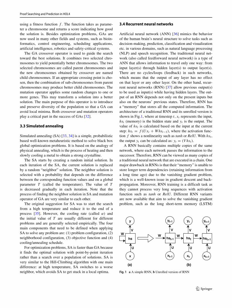
Artificial neural network (ANN) [36] mimics the behaviorof the human brain’s neural structure to solve tasks such asdecision-making, prediction, classification and visualizationetc. in various domains, such as natural language processing(NLP) and speech recognition. The traditional neural net-work (also called feedforward neural network) is a type ofANN that allows information to travel only one way: frominput layer(s) through hidden layer(s) to output layer(s).There are no cycles/loops (feedback) in such networks,which means that the output of any layer has no effecton that layer or any other layer. On the other hand, recur-rent neural networks (RNN) [37] allow previous output(s)to be used as input(s) while having hidden layers. The out-put of an RNN depends not only on the present inputs butalso on the neurons’ previous states. Therefore, RNN hasa “memory” that stores all the computed information. Thearchitecture of a traditional RNN and its unrolled version isshown in Fig.1, where at timestep t , xt represents the input,hst (memory) is the hidden state and yt is the output. Thevalue of hst is calculated based on the input at the currentstep: hst = f (Uxt + Whst−1), where the activation func-tion f shows a nonlinearity such as tanh or RelU. With hst ,the output yt can be calculated as: yt = (V hst ).

A RNN basically contains multiple copies of the samenetwork, where each network passes the information to thesuccessor. Therefore, RNN can be viewed as many copies ofa traditional neural network that are executed in a chain. Onemajor drawback in RNNs is that their “memory” is unable tostore longer term dependencies (retaining information froma long time ago) due to the vanishing gradient problem,which is a well-known issue in gradient descent and back-propagation. Moreover, RNN training is a difficult task asthey cannot process very long sequences with activationfunction such as tanh or RelU. Different RNN variantsare now available that aim to solve the vanishing gradientproblem, such as the long short-term memory (LSTM)

x

hs

y

(a) (b)

V

U

W

xt-1

hst-1

yt-1

V

U

W

xt

hst

yt

V

U

W

xt+1

hst+1

yt+1

V

U

W

Fig. 1 a A simple RNN, b Unrolled version of RNN

M. Saqib Nawaz et al.

network [38]. In this paper, we propose to use LSTM forthe considered problem and more details about LSTM areprovided in Section 6.

4 Proof searching approaches

The proposed structure (flowchart) of the evolutionary andheuristic-based approaches that is used to find and optimizethe proofs of theorems/lemmas in HOL4 theories is shownin Fig. 2.

The proof development process in HOL4 is interactive innature and it follows the lambda calculus proof represen-tation. Proofs in HOL4 are constructed with an interactivegoal stack and then put together using the ML functionprove. A user first provides the property (in the form of alemma or theorem) that is called a proof goal. A proof goalis a sequent that constitutes a set of assumptions and con-clusion(s) as HOL formulas. Then the user applies proofcommands and tactics to solve the proof goal. A tactic isbasically a function that takes a proof goal and returns asub-goals together with a validation function. The actionresulting from the application of a proof command and tac-tics is referred to as a HOL4 proof step (HPS). A HPSmay either prove the goal or generate another proof goalor divide the main goal into sub-goals. The proof develop-ment process for a theorem or lemma is completed whenthe main goal or all the sub-goals are discharged fromthe goal stack. The fact that the proof script of a partic-ular theorem or lemma depends on the application of theHPS in a specific order makes automatic proof search fora goal quite challenging. However, evolutionary and heuris-tic algorithms have the potential to search for the proofs of

Create an initial populationfrom HOL4 proof steps

Random generation of proofsequences from population

Crossover and mutationoperators

Stoppingcriteria

YesNo

Determine the fitness of theproof sequence

(a) GA

Create an initial populationfrom HOL proof steps

Generate a random proofsequence�

Simulated Annelaing

Stoppingcriteria

YesNo

(b) SA

Fig. 2 Flowchart of proof searching approaches in HOL4

theorems/lemmas due to their ability to handle black-boxsearch and optimization problems.

We propose to convert the data available in HOL4 prooffiles to a proper computational format so that a GA and SAcan be used. Moreover, the redundant information (relatedto HOL4) that plays no part in proof searching and evolutionis removed from the proof files. The complete proof for agoal (theorem/lemma) can now be considered as a sequenceof HPS. Let PS = {HPS1, HPS2, . . . HPSm} representthe set of HPS proof steps. A proof step set PSS is aset of HPS, that is PSS ⊆ PS. Let the notation |PSS|denote the set cardinality. PSS has a length n (calledn-PSS) if it contains n proof commands, i.e., |PSS| =n. For example, consider that PS = {RW, PROVE TAC,

FULL SIMP TAC, REPEAT GEN TAC, DISCH TAC}. Now, theset {RW, FULL SIMP TAC, REPEAT GEN TAC} is a proof stepset that contains three proof steps. A proof sequence is alist of proof step sets S = 〈PSS1, PSS2, ..., PSSn〉, suchthat PSSi ⊆ PSS (1 ≤ i ≤ n). For example, 〈{RW,PROVE TAC}, {FULL SIMP TAC}, {GEN TAC, DISCH TAC}〉 isa proof sequence, which has three PSS and five HPS that areused to prove a theorem/lemma.

A proof dataset PD is a list of proof sequences PD=〈S1,

S2, ..., Sp〉, where each sequence has an identifier (ID). Forexample, Table 1 shows a PD that has five proof sequences.

4.1 Proposed genetic algorithm (GA)

Algorithm 1 presents the pseudocode of the proposed GAthat is used to find the proofs in the HOL4 theories. Itcontains the HPS used for the verification of theorems andlemmas in the considered theories.

Proof Searching and Prediction in HOL4

Table 1 A sample proof datasetID Proof Sequence

1 〈{GEN TAC, CONJ TAC, MP TAC}〉2 〈{GEN TAC, X GEN TAC, PROVE TAC}〉3 〈{RW, PROVE TAC, CONJ TAC, MAP EVERYTHING TAC, AP TERM TAC}〉4 〈{GEN TAC, SUBGOAL THEN, DISCH TAC, CASES ON, AP TERM TAC, BETA TAC, CASES TAC}〉5 〈{RW TAC, SUBST1 TAC, Q.SUBGOAL THEN, SRW TAC, FULL SIMP TAC}〉

An initial population (Pop) is first created from frequentHPS (FHPS) that are discovered with various sequentialpattern mining (SPM) techniques [39]. Based on this initialpopulation, two random proof sequences (P1 and P2) aregenerated and are passed through the crossover operationwhere the child proof sequences are generated and theirfitness is evaluated. The mutation operation is applied to thechild having the better fitness value to generate the mutatedchild sequence.

If a mutated child’s fitness is equal to the fitness ofthe target proof sequence from PD, then the mutated childis returned as the final proof sequence. The process ofcrossover and mutation continues until randomly generatedproof sequences exactly match the proof sequences fromthe PD. The fitness values guide the GA toward thebest solution(s) (proof sequences). Here the fitness valuerepresents the total number of HPS in the random proofsequence that match the HPS in the position of the original(target) proof sequence. Algorithm 2 presents the procedurefor calculating the fitness value of a proof sequence.

In each generation, the priority of the randomly generatedproof sequence is ranked according to the fitness valuescalculated based on the above mentioned fitness procedure.This procedure evaluates how close a given solution is tothe optimum solution (in our case, the target solution). Itcompares each gene i of a random proof sequence (Pseq)with the genes of the target (P). The fitness of PSeq is set

to 0, and increased by 1 for each matching gene and if thegenes in both sequences are equal then the fitness of 1 isassigned. For example, consider the following random proofsequence (RP) and the target sequence (TP):

RP = MAP EVERYTHING TAC, RULE ASSUM TAC,

X GEN TAC, SRW TAC, AP TERM TAC,

DISCH TAC, DECIDE TAC, RW TAC

TP = POP ASSUM, REAL ARITH TAC, X GEN TAC,

COND CASES TAC, AP TERM TAC,

RULE ASSUM TAC, X GEN TAC, RW TAC

The Fitness procedure returns 3 as three HPS are the samein both sequences (at Positions 3, 5 and 8, respectively).

Algorithm 3, 4 and 5 present the pseudocode of the threecrossover operators. The symbol o in these algorithms rep-resents the concatenation. These three crossover proceduresare explained with simple examples. Let P1 and P2 be:

P1 = SRW TAC, MAP EVERYTHING TAC, X GEN TAC,

AP TERM TAC, RULE ASSUM TAC, DISCH TAC,

DECIDE TAC, RW TAC

P2 = REAL ARITH TAC, POP ASSUM, X GEN TAC,

COND CASES TAC, RW TAC,

RULE ASSUM TAC, X GEN TAC, AP TERM TAC

Let n represents the length of both proof sequencesand let position cp (1 ≤ cp ≤ n) be chosen randomlyas crossing point in both proof sequences. Single pointcrossover (SPC) produces the following proof sequences forcp = 4:

P ′1 = SRW TAC, MAP EVERYTHING TAC, X GEN TAC,

COND CASES TAC, RW TAC, RULE ASSUM TAC,

X GEN TAC, AP TERM TAC

P ′2 = REAL ARITH TAC, POP ASSUM, X GEN TAC,

AP TERM TAC, RULE ASSUM TAC, DISCH TAC,

DECIDE TAC,RW TAC

Fitness of newly generated sequences are checked lastand SPC returns the proof sequence having the highestfitness.

M. Saqib Nawaz et al.

Two crossing points are selected by the multi pointcrossover (MPC) operator. Let cp1 and cp2 represent twocrossing points (cp1 < cp2 ≤ n). For P1 and P2, the newproof sequences generated for cp1 = 4 and cp2 = 5 are:

P ′1 = SRW TAC, MAP EVERYTHING TAC, X GEN TAC,

COND CASES TAC, RW TAC, DISCH TAC,

DECIDE TAC, RW TAC

P ′2 = REAL AIRTH TAC, POP ASSUM, X GEN TAC,

AP TERM TAC, RULE ASSUM TAC,

RULE ASSUM TAC,X GEN TAC, AP TERM TAC

Newly generated sequences are evaluated last and MPC

returns the proof sequence having the highest fitness.In uniform crossover (UC), each element (gene) of the

proof sequences is assigned to the child sequences with aprobability value p. UC evaluates each gene in the proofsequences and selects the value from one of the proofsequences with the probability p. If p is 0.5, then the childhas approximately half of the genes from the first proofsequence and the other half from the second proof sequence.For P1 and P2, some newly generated proof sequences afterUC with p = 0.5 are:

P ′1 = SRW TAC, POP ASSUM, X GEN TAC,

COND CASES TAC, RULE ASSUM TAC,

DISCH TAC, X GEN TAC, RW TAC

P ′2 = REAL ARITH TAC, MAP EVERYTHING TAC,

X GEN TAC, AP TERM TAC, RW TAC,

RULE ASSUM TAC, DECIDE TAC,

AP TERM TAC

Because UC is a randomized algorithm, depending on theselection probability, the generated child proof sequencescan be different. Fitness of newly generated sequences is

then checked and the UC returns the sequence having thehighest fitness.

The mutation operation is applied after the crossoveroperation. The standard mutation (SM) operator of GAsadds random information to the search process, so that itdoes not get stuck in a local optima. In SM, the selectedlocation value is changed from its original value with someprobability, called mutation probability, and is denoted as

Proof Searching and Prediction in HOL4

pm. For a proof sequence, a randomly chosen genes valuei is replaced by a random HPS from the current populationPop. For example, a mutation of the proof sequence P1 is:

P ′1 = SRW TAC, POP ASSUM, X GEN TAC,

DECIDE TAC,RULE ASSUM TAC,

DISCH TAC, X GEN TAC,RW TAC

The pairwise interchange mutation (PIM) operatorselects and interchanges two arbitrary genes from a proofsequence. But for proof searching, we empirically observedthat a GA could not find the target proof sequence withPIM as it was only interchanging the values betweentwo genes in the random proof sequence. To address thisissue, we revised the PIM procedure such that the twoselected gene values are replaced by random HPS fromthe population rather than interchanging the values. Forinstance, by applying modified PIM on the proof sequenceP1, the following mutated proof sequence can be obtained:

P ′1 = SRW TAC, REWRITE TAC, X GEN TAC,

DECIDE TAC, RULE ASSUM TAC, BETA TAC,

X GEN TAC, RW TAC

The reason to use more than one crossover and mutationoperators is to investigate their effect on the overallperformance of the GA in proof searching. It is important

to point out that in each generation, a random proofsequence goes through crossover and mutation operationwith a probability of 1 to reduce the number of iterationsperformed by the GA.

4.2 Simulated annealing (SA)

Algorithm 8 presents the proposed pseudocode of the SAthat is used to find the proofs in HOL4 theories.

Just like GA, an initial population (Pop) is first createdfrom FHPS. From this population, a random proof sequence(PS) is then generated that is passed through the annealingprocess (Steps 9-25 in Algorithm 8), where it is evolveduntil its fitness is equal to the fitness of the targetproof sequence from PD. Besides annealing, the algorithmconsists of two main procedures, Fitness and Get Neighbor(GN), which are explained next.

Fitness values guide the SA toward the best solution(s)(proof sequences). Here the fitness value is the total numberof HPS in the random proof sequence that matches theHPS in the position of the original (target) proof sequence.Algorithm 2 (from Section 4.1) presents the procedure forcalculating the fitness value of a proof sequence.

M. Saqib Nawaz et al.

In the annealing process, a neighbor random sequenceis first generated. Algorithm 9 presents the procedure forgetting the neighbor solution. The selected location valueis changed from its original value in the Get Neighbor.For a proof sequence, a randomly chosen genes value i isreplaced by a random HPS from the current population Pop.It is important to point out here that the standard mutationoperator of GA and the get neighbor procedure in SA arequite similar.

After the Get Neighbor procedure, the fitness of theneighbor solution is calculated. The randomly generatedproof sequence and the neighbor sequence is then com-pared. If the fitness of the neighbor is better, then it isselected. Otherwise, an acceptance rate (Step 19 in Algo-rithm 8) is used to select one out of the two sequences.The acceptance rate depends on temperature. Finally, thetemperature Temp is decreased with the following formula:

Temp = Temp × α

where the value of α is in the range of 0.8 < α < 0.99. Theprocess of annealing is repeated (Steps 9-24 in Algorithm8) until the random proof sequence fitness matches with thetarget proof sequence or Temp reaches the minimum value(Temp min). In our case, we set the value of Temp such thatthe SA always terminates when the random proof sequencematches with the target proof sequence. The process thatdistinguishes SA from GA is the annealing process.

Besides the annealing process, another main concept inSA is the acceptance probability. SA checks whether thenew solution is better than the previous solution. If thenew solution is worse than the present solution, it may stillpick the new solution with some probability known as theacceptance probability that governs whether to switch tothe worst solution or not. This way, we may avoid the localoptimum by exploring other solutions. Now this may seemworse or unacceptable at present, but it could lead SA to theglobal optimum. For this purpose, we chose the acceptanceprobability by using acceptance rate (AR) formula as:

AR = exp

(T

1 + T

)

where T is the current temperature. We performed experi-ments to check the effect of AR on the performance of SAfor proof searching. From the simulation results presented inthe next section, it was observed that this parameter effectsthe performance of SA, but it is negligible.

5 GA and SA based results and discussion

The proposed GA and SA algorithms, described in theprevious section, are implemented in Python and the codecan be found at [40]. To evaluate the proposed approaches,experiments were carried on a fifth generation Core i5processor and 8 GB of RAM. Some initial and importantresults obtained by applying the proposed GA and SA basedapproaches on PD are discussed in this section.

We first investigated the performance of the proposedGA for finding the proofs of theorems in 14 HOL4 theoriesavailable in its library. These theories are: Transcenden-tal, Arithmetic, RichList, Number, Sort, Bool, BinaryWords,FiniteMap, InductionType, Combinator, Coder, Encoder,Decoder and Rational. We selected five to twenty the-orems/lemmas from each theory and in total, we haveproof sequences for 300 theorems/lemmas and 89 distinctHPS in the PD. Table 2 lists some of the important theo-rems/lemmas from the theories. For example, L1 (Lemma 1)from the transcendental theory proves the property for theexponential bound of a real number x. Similarly, T2 is thetheorem for the positive value of sine when the given valueis in the range [0 − 2]. T10 from the Rational theory is thedense theorem that proves that there exists a rational numberbetween any two real numbers.

The GA was run with the different crossover andmutation operators on the considered theorems/lemmas tentimes. Fitness values in Table 3 represent the total HPS thatis used in the complete proof and this value is kept thesame for respective theorems and lemmas in all crossoverand mutations operators. The generations column showshow many times a random proof sequences goes throughGA operators to reach the target proof sequence. The timecolumn represents how much time (in seconds) is taken bythe GA to find the complete proof for a theorem. We foundthat different crossover operators with the same mutationoperator required almost the same number of generations tofind the target proofs. However, with MPIM (Algorithm 7),the target proofs are found in less generations as comparedto SM (Algorithm 6). It is important to point out that theprobability in UC (Algorithm 5) has no noticeable effect onthe average generation count of the GA. That is why weselect the probability (p = 0.5) for UC.

Just like GA, we investigate the performance of theproposed SA for finding the proofs of theorems/lemmasin 14 HOL4 theories and the obtained results are listed in

Proof Searching and Prediction in HOL4

Table 2 A sample oftheorems/lemmas in six HOL4theories

HOL Theory No. HOL4 Theorems

L1 ∀x. 0<=x∧xv<= inv(2) ==> exp(x) <= 1+2*x

Transcendental T1 ∀ x. (\n. (∧exp ser) n (x pow n)) sums exp(x)

T2 ∀ x. 0 < x∧ x < 2 ==> 0 < sin (x)

Arithmetic T3 ∀n a b. 0 < n ==>((SUC a MOD n = SUC b MOD n)

= ( a MOD n = b MOD n ))

RichList T4 ∀m n. ((l:’a list). ((m + n)=(LENGTH l))==>

( APPEND ( FIRSTN n l ) ( LASTN m l ) = l)

T5 ∀n m. ( m <= n ==> (iSUB T n m = n - m)) ∧Number (m < n ==> (iSUB F n m = n - SUC m))

T6 ∀ n a. 0 < onecount n a ∧ 0 < n ==>

( n = 2 EXP (onecount n a - a ) - 1 )

Sort T7 (PERM L [x] = (L = [x]))∧(PERM [x] L = (L = [x]))

T8 PERM = TC PERM SINGLE SWAP

T9 ∀ x y. abs rat ( frac add ( rep rat (

Rational abs rat x ) ) y ) = abs rat ( frac add x y )

T10 ∀ r1 r3. rat les r1 r3 ==> ?rat res r1 r2

∧ rat les r2 r3

Table 4. The comparison of SA with GA for T2 is shown inthe second part of Table 4. For the GA, a different crossoveroperator has no great effect on the overall performance ofthe GA. However, using the MPIM operator allowed to findthe target proof sequences considerably more quickly thanusing the SM operator. For T2, SA is found to be faster(30232 generations) than the GA with different crossoverand mutation operators. For this particular example, SAis approximately sixty times faster than GA with differentcrossover operators and SM. Whereas, it is approximatelyten times faster than the GA with different crossoveroperators and MPIM.

The average number of generations for the SA andGA with different crossover and mutation operators toreach the target proof sequences in the whole dataset areshown in Table 5. GA with different crossover and MPIMoperators is approximately fourteen times faster than theGA with different crossover operators and SM. A possibleexplanation for this is that the SM changes the HPS at asingle location of the sequence, while MPIM changes twolocations. Thus, MPIM explores a more diverse solutionas compared to SM. Whereas, SA is six times faster thanGA with MPIM and different crossover operators. The mainreasons for this is that in SA, only one procedure (GN) iscalled. On the other hand, in GA, two procedures (crossoverand mutation) are called.

Population diversity greatly influences a GA’s ability topursue a fruitful exploration as it iterates from a generationto another [41]. The proof searching process with GA can betrapped in a local optima due to the loss of diversity throughpremature convergence of the HPS in the population. Thismakes the diversity maintenance and computation one of

the fundamental issues for the GA. We studied populationdiversity with two measures. The first one being thestandard deviation of fitness SDf , whose values in the Popof HPS is measured as:

SDf =√∑N

i=1(fi − f )2

N − 1

where N is the total number of proof sequences, fi is thefitness of the ith proof sequence and f is the mean of thefitness values. As the fitness values for random proof sequencesremain the same (after evolution) for all crossover andmutation operators, so SDf is 14.12 with a mean of 12.05for the GA. The second measure that is used to investigatethe variability of HPS in Pop and the extent of deviation(dispersion) for the proof sequences as a whole is thestandard deviation of time (SDt ), which is measured as:

SDt =√∑N

i=1(ti − t )2

N − 1

where ti is the time taken by the GA to find the correct ith

proof sequence and t is the mean of the time values.Table 6 lists the calculated SDt for all the proofs in

the PD along with their mean for different crossover andmutation operators. A low SD indicates that the data (timevalues to find respective HPS in proof sequences) is lessspread out and is clustered closely around the mean averagevalues. Whereas a high SD means that the data is spreadapart from the mean. SM is found to be approximatelyfourteen times slower than MPIM. That is why we havemore time points for SM than MPIM, which makes the SDt

and the respective mean higher for SM.

M. Saqib Nawaz et al.

Table 3 Results for the proposed GA

T/L C∗ & M∗ Fit∗∗ Generations Time(s) C & M Fit Generations Time (s)

L1 SPC/SM 54 1,903,765 55.43 SPC/MPIM 54 314,043 9.52

T1 SPC/SM 58 2,103,765 60.10 SPC/MPIM 58 334,043 10.33

T2 SPC/SM 81 1,947,597 93.56 SPC/MPIM 81 392,822 12.89

T3 SPC/SM 66 2,473,394 62.35 SPC/MPIM 66 191,162 6.61

T4 SPC/SM 19 297,179 4.72 SPC/MPIM 19 38,307 0.93

T5 SPC/SM 23 501,813 8.30 SPC/MPIM 23 33,655 0.71

T6 SPC/SM 30 709,484 13.09 SPC/MPIM 30 34,776 0.79

T7 SPC/SM 17 264,263 4.11 SPC/MPIM 17 21,136 0.40

T8 SPC/SM 42 811,951 28.49 SPC/MPIM 42 39,302 1.41

T9 SPC/SM 23 554,111 9.30 SPC/MPIM 23 45,309 0.90

T10 SPC/SM 23 546,136 9.21 SPC/MPIM 23 51,552 1.01

L1 MPC/SM 54 1,488,005 27.21 MPC/MPIM 54 105,521 3.29

T1 MPC/SM 58 1,540,467 35.93 MPC/MPIM 58 153,644 5.01

T2 MPC/SM 81 1,898,305 80.38 MPC/MPIM 81 191,699 7.69

T3 MPC/SM 66 1,128,636 31.54 MPC/MPIM 66 104,784 3.60

T4 MPC/SM 19 358,182 7.01 MPC/MPIM 19 24,960 0.48

T5 MPC/SM 23 384,539 7.19 MPC/MPIM 23 42,750 0.83

T6 MPC/SM 30 738,037 10.21 MPC/MPIM 30 73,408 1.13

T7 MPC/SM 17 276,087 5.32 MPC/MPIM 17 19,997 0.43

T8 MPC/SM 42 1,245,801 25.67 MPC/MPIM 42 101,795 2.52

T9 MPC/SM 23 411,625 7.73 MPC/MPIM 23 275,78 0.63

T10 MPC/SM 23 480,625 8.26 MPC/MPIM 23 25,314 0.55

L1 UC/SM 54 1,652,013 61.83 UC/MPIM 54 63,277 1.86

T1 UC/SM 58 1,682,200 68.32 UC/MPIM 58 126,097 2.92

T2 UC/SM 81 2,348,878 101.63 UC/MPIM 81 312,328 8.21

T3 UC/SM 66 1,662,751 44.81 UC/MPIM 66 257,215 7.48

T4 UC/SM 19 706,950 11.12 UC/MPIM 19 20,702 0.41

T5 UC/SM 23 819,903 14.97 UC/MPIM 23 71,614 1.37

T6 UC/SM 30 867,183 17.21 UC/MPIM 30 74,635 1.53

T7 UC/SM 17 321,183 6.16 UC/MPIM 17 20,263 0.42

T8 UC/SM 42 804,969 20.53 UC/MPIM 42 29,606 0.95

T9 UC/SM 23 625,908 11.38 UC/MPIM 23 130,303 2.50

T10 UC/SM 23 716,950 13.07 UC/MPIM 23 90,425 1.94

∗ Crossover and mutation ∗∗ Fitness

We also checked the amount of memory used by GA(shown in Table 6) while searching for proofs. Moreover, wenoticed that the GA using different crossover and mutationoperators requires approximately the same memory whilesearching for proofs and their optimization in PD.

With acceptance probability, SA may accept a newsolution obtained with the GN procedure that is worstthan the present solution. The reason for this is that thereis always a possibility that the worst solution could leadthe SA to the global optimum. In our proposed SA, wechose the acceptance probability with the AR formula (AR= exp( T

1+T)). This AR is then compared with a random

number generated within the range (2.71820060604849,2.71825464604849).

The range is selected after experimenting with the fol-lowing values: T emp = 100000.0, T emp min = 0.00001,and α = 0.99954001. If the value of AR is greater than therandom number generated within the above range, then theworse solution is going to be picked. We also used a counternamed acceptance rate counter (ARC) that counts how manytimes the worst solution is picked. By simulation, we cameto know that this factor does not play any significant rolein the overall generation count or time. This is because ofthe fact that in our case, we do not have any local optimum.

Proof Searching and Prediction in HOL4

Table 4 Results for SA and comparison with GA

T/L Fitness Generations Time (s)

L1 54 17,636 0.56

T1 58 21,144 0.82

T2 81 30,232 1.11

T3 66 22,919 0.65

T4 19 3,924 0.10

T5 23 5,057 0.09

T6 30 4,370 0.08

T7 17 1,892 0.02

T8 42 16,767 0.32

T9 23 7,734 0.16

T10 23 6,997 0.14

T2 GA(SPC/SM) 1,947,597 93.56

T2 GA(MPC/SM) 1,898,305 80.38

T2 GA(UC/SM) 2,348,878 101.63

T2 GA(SPC/MPIM) 392,822 12.89

T2 GA(MPC/MPIM 191,699 7.69

T2 GA(UC/MPIM) 312,328 8.21

SPC = single point crossover, MPC = multi point crossover, UC= uniform crossover, SM = standard mutation, MPIM = modifiedpairwise interchange mutation

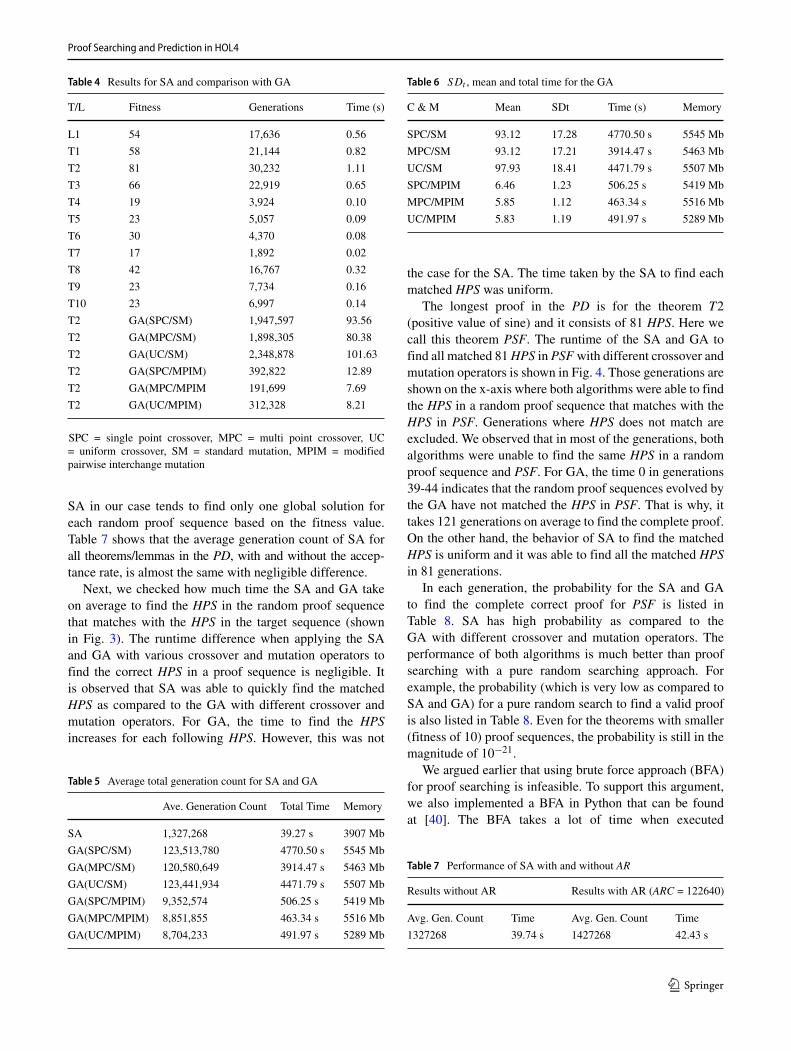
SA in our case tends to find only one global solution foreach random proof sequence based on the fitness value.Table 7 shows that the average generation count of SA forall theorems/lemmas in the PD, with and without the accep-tance rate, is almost the same with negligible difference.

Next, we checked how much time the SA and GA takeon average to find the HPS in the random proof sequencethat matches with the HPS in the target sequence (shownin Fig. 3). The runtime difference when applying the SAand GA with various crossover and mutation operators tofind the correct HPS in a proof sequence is negligible. Itis observed that SA was able to quickly find the matchedHPS as compared to the GA with different crossover andmutation operators. For GA, the time to find the HPSincreases for each following HPS. However, this was not

Table 5 Average total generation count for SA and GA

Ave. Generation Count Total Time Memory

SA 1,327,268 39.27 s 3907 Mb

GA(SPC/SM) 123,513,780 4770.50 s 5545 Mb

GA(MPC/SM) 120,580,649 3914.47 s 5463 Mb

GA(UC/SM) 123,441,934 4471.79 s 5507 Mb

GA(SPC/MPIM) 9,352,574 506.25 s 5419 Mb

GA(MPC/MPIM) 8,851,855 463.34 s 5516 Mb

GA(UC/MPIM) 8,704,233 491.97 s 5289 Mb

Table 6 SDt , mean and total time for the GA

C & M Mean SDt Time (s) Memory

SPC/SM 93.12 17.28 4770.50 s 5545 Mb

MPC/SM 93.12 17.21 3914.47 s 5463 Mb

UC/SM 97.93 18.41 4471.79 s 5507 Mb

SPC/MPIM 6.46 1.23 506.25 s 5419 Mb

MPC/MPIM 5.85 1.12 463.34 s 5516 Mb

UC/MPIM 5.83 1.19 491.97 s 5289 Mb

the case for the SA. The time taken by the SA to find eachmatched HPS was uniform.

The longest proof in the PD is for the theorem T2(positive value of sine) and it consists of 81 HPS. Here wecall this theorem PSF. The runtime of the SA and GA tofind all matched 81 HPS in PSF with different crossover andmutation operators is shown in Fig. 4. Those generations areshown on the x-axis where both algorithms were able to findthe HPS in a random proof sequence that matches with theHPS in PSF. Generations where HPS does not match areexcluded. We observed that in most of the generations, bothalgorithms were unable to find the same HPS in a randomproof sequence and PSF. For GA, the time 0 in generations39-44 indicates that the random proof sequences evolved bythe GA have not matched the HPS in PSF. That is why, ittakes 121 generations on average to find the complete proof.On the other hand, the behavior of SA to find the matchedHPS is uniform and it was able to find all the matched HPSin 81 generations.

In each generation, the probability for the SA and GAto find the complete correct proof for PSF is listed inTable 8. SA has high probability as compared to theGA with different crossover and mutation operators. Theperformance of both algorithms is much better than proofsearching with a pure random searching approach. Forexample, the probability (which is very low as compared toSA and GA) for a pure random search to find a valid proofis also listed in Table 8. Even for the theorems with smaller(fitness of 10) proof sequences, the probability is still in themagnitude of 10−21.

We argued earlier that using brute force approach (BFA)for proof searching is infeasible. To support this argument,we also implemented a BFA in Python that can be foundat [40]. The BFA takes a lot of time when executed

Table 7 Performance of SA with and without AR

Results without AR Results with AR (ARC = 122640)

Avg. Gen. Count Time Avg. Gen. Count Time

1327268 39.74 s 1427268 42.43 s

M. Saqib Nawaz et al.

0

0.1

0.2

0.3

0.4

0.5

0.6

1 2 3 4 5 6 7 8 9 10

Tim

e (S

ec)

Number of HPS

SPC/SM

MPC/SM

UC/SM

SPC/MPIM

MPC/MPIM

UC/MPIM

SA

Fig. 3 Time used by the SA and GA to find the first ten matched HPS

on proof sequences in the PD, even for theorems withsmaller fitness values. For example, Table 9 lists the resultsobtained with the BFA. The attempts column shows howmany times (iterations) the approach tried to find the targetproof sequence. For a theorem with a fitness value of4, it took 124 seconds and 13239202 attempts, that isapproximately 106767 attempts per second, to find thetarget proof sequence.

For a theorem with a fitness value of 6, the program keptrunning for more than 50 hours and it was still unable to findthe target proof sequence.

Overall, it was observed through various experiments thatthe proposed GA and SA are able to quickly optimize andautomatically find the correct proofs for theorems/lemmasin different HOL4 theories. SA was observed to be muchfaster than GA and in turn utilized less memory. Besides

0

5

10

15

20

25

30

35

1 6 11 16 21 26 31 36 41 46 51 56 61 66 71 76 81 86 91 96 101 106 111 116 121

Tim

e (S

ec)

Genera�ons

SPC/SM

MPC/SM

UC/SM

SPC/MPIM

MPC/MPIM

UC/MPIM

SA

Fig. 4 Total time and generations for the PSF theorem with SA and GA

Proof Searching and Prediction in HOL4

Table 8 Comparison of SA, GA and Pure Random Search (PRS)

Algorithm Probability

SA 2.12 × 10−3

GA(CO/SM) 4.84 × 10−6

GA(CO/MPIM) 5.04 × 10−5

PRS 1.62 × 10−197

HOL4, both evolutionary and heuristic based approachescan also be used for proof searching and proof optimizationin other proof assistants, such as Coq [4] and PVS [5].

6 Proof learning with LSTM

The proof searching approaches in Section 4 are unableto learn the proof process. They are efficient in evolvingrandom proof sequences to target proof sequences. Themain focus now in theorem provers, particularly in ITPs,is to make the proof development process as automatic aspossible. This will not only ease the proving process forusers but also reduce the time and efforts users spend whileinteracting with ITPs. In this context, proof learning andprediction is an important task. With the advancement andevolution in computing capabilities and the fast progressin deep learning techniques, we believe that RNNs aresuitable to provide an effective proof learning mechanismfor formal proofs because of their instrumental successin the AlphaGo [42] and usefulness in the tasks relatedto logical inference and reasoning [43, 44], automatedtranslation [45], conversation modeling [46] and knowledgebase completion [47]. Therefore, we propose to use a variantof RNN known as LSTM for the task of proof learning.

During the proof development process, HOL4 users arerequired to formalize their inputs with (1) HPS, and (2)arguments for those HPS. For example, the tactic (HPS)DISCH TAC moves the antecedent of an implicative goalinto assumptions. Similarly, GEN TAC strips the outermostuniversal quantifier from the conclusion of a goal. Tacticarguments (called dependencies in [16]) provide moredetailed information about HPS. For example, the HPSInduct on ‘n‘ applies induction on a variable n. In theproposed proof learning and prediction with RNN, we focuson HPS only. Since automatic reasoning in ITPs is a hard

Table 9 Results for BFAProof Sequence Fit Time Attempts

GEN TAC REWRITE TAC 2 0.001 s 67

STRIP TAC SRW TAC METIS TAC 3 0.078 s 4292

GEN TAC BETA TAC Q.SPEC TAC ASM REWRITE TAC 4 124 s 13239202

RW TAC CASES ON CASES ON FULL SIMP TAC PROVE TAC 5 4412s 922370015

problem due to the undecidability of the underlying higher-order logic [48, 49], the aim is not to provide the supportfor fully automated reasoning. Instead, our aim is to providean approach that can analyze existing HOL4 proofs to learnthe proof process and on the basis of learning, predictproof-steps/tactics (HPS).

RNNs have a simple structure of repeating units thatallows the flow of information. Standard RNNs are usuallybuilt with tanh activation function as shown in Fig. 5a.With xt , hst and yt as the input, hidden state and outputrespectively, the hst and yt for the unit t can be calculatedas:

hst = tanh(Wxhsxt + Whshshst−1 + bhs), (1)

yt = (Wyhshst + by) (2)

where Wxhs , Whshs and Wyhs represent the weight variablefor input, hidden unit and output, respectively, and bhs , by

are the biases in the unit.In principle, RNNs can store and manipulate past

information to produce the desired information as output.As we are dealing with long proofs sequences, RNNs are notsuitable for learning and prediction due to their short termmemory and the vanishing gradient problem [50].

This problems occurs when RNNs are trained withgradient based methods (e.g back-propagation). It describesthe situation where RNNs are unable to propagate usefulgradient information from the output end back to the layersnear the input end. As more layers are added, the gradientsapproach zero, making the network hard to train.

For example, the derivative of the gradient that passesthrough the tanh activation function is smaller than 1 forall inputs except 0. Then the state of the unit t can berepresented as:

hst = tanh(Wxhsxt + Whshshst1 + bhs)

= tanh(Wxhsxt + Whshs tanh(Wxhsxt1

+Whshshst2 + bhs))

= .................

with the increase in t , the effect of x1 keeps decreasing,which apparently contributes to the vanishing gradientproblem.

One way to avoid the problem is to use ReLU in placeof the tanh or sigmoid (σ ) function. However, ReLU helps

M. Saqib Nawaz et al.

Fig. 5 Difference between RNNand LSTM (Figures courtesy of[51])

(a) RNN cell (b) LSTM cell

in avoiding the problem but does not rectify the problemcompletely.

LSTMs [38] are RNNs that are explicitly designed toavoid the long-term dependency problem. Rememberinginformation for long periods of time is practically theirdefault behavior. LSTMs have a chain like structure (similarto RNNs), but with different unit: four neural network layersinstead of a single one as shown in Fig. 5b. A LSTM cellhas 3 gates: (1) Input gate, (2) Forget gate, and (3) Outputgate. Each gate is a layer with an associated weight and bias(for example, Wf and bf for the forget gate, Wi and bi forthe input gate and Wo and bo for the output gate).

The forget gate decides whether to keep the informationfrom previous hidden state or to delete it. This decision ismade by a sigmoid layer in the forget gate that looks atthe previous hidden state (hst−1) and current input (xt ), andoutputs a number between 0 (means to keep information)and 1 (means to delete information). The input gate decideswhether a given information is worth remembering and theσ in this layer decides which value to update. The outputgate decides whether the information at a given step isimportant and should be used or not. Let ft , it and ot

represents the output of forget gate, input gate and outputgate layers respectively, then:

ft = σ(Wf .[hst−1, xt ] + bf ) (3)

it = σ(Wi .[hst−1, xt ] + bi) (4)

ot = σ(Wo.[hst−1, xt ] + bo) (5)

Besides three gates, there is a tanh layer between theinput and output gates that creates a vector of new candidate(temporal) values (denoted as Ct ) for the current time step,which can be added to the state. The new cell state (Ct ) is

calculated with Ct , old cell state (Ct−1), ft and it . Finally,the output of the LSTM cell is based on the tanh layer(between output gate and cell state) and ot . It is importantto point out that the σ in the output gate layer decides whichinformation from the cell state will go to the output. Thenew cell state finally passes through tanh to push its valuesin between -1 and 1.

Ct = tanh(WC .[hst−1, xt ] + bC) (6)

Ct = ft × Ct−1 + it + Ct (7)

Yt = ot × tanh(Ct ) (8)

where . is the dot product operator (between vectors), ×is the pointwise multiplication operator (between a realnumber and a vector) and [y, z] is the concatenationoperator (between vectors).

The dataset PD contains the proof sequences, where eachline represents the proof sequence for one theorem/lemma.The dataset is pre-processed further, where each line thatcontains HPS is split into lists of characters that aretransformed into vectors (tensors) so that LSTM can processthem one by one. Each character in HPS is mapped to adistinct number {char → number}. The character with alow number indicates that the respective character is morepopular (occurs more) among others in the PD. In the tensor,the characters in a HPS are replaced with their respectivenumber. For example, the tactic GEN T AC is transformedinto the following tensor:

GEN T AC → [28 46 4 5 15 11 19]The main reason why the arguments for HPS is not

selected is that these parameters depends on the specifica-tion (particularity on variables and functions declarations)

Proof Searching and Prediction in HOL4

inside the theory and on the proof goal. This means thatarguments for a particular HPS can be different for differ-ent theories and different proof goals. During the reasoningprocess in HOL4, a proof goal can be considered as acontext-HPS pair, where context contains the informationabout the current hypotheses, variables and the goal thatneeds proving. The goal may contains a set of subgoals. Theuser is required to guide the proof process towards comple-tion by suggesting which HPS (and arguments) to use. Webelieve that adding arguments information would restrict thelearning model to work well for only one (or some related)theory. Moreover, it will also add more complexity and willincrease the computation time for the model.

Our aim is to train the LSTM model in such a way thatfor a given input, the model generates the desired output.For that, the created tensor is divided into input and output(target) batches. Let us assume (for simplicity) that the totallength of the proof sequence is 8. For this sequence, thefirst input batch can be set to 5 initial tensor values. Ourrequirement from the model is to predict the next characterfor a list of previous characters. This requirement can besatisfied by creating a target batch that subscripts the tensorwith a n + 1 shift compared to the input batch, where n

represents the length of input batch. Table 10 shows howthe model predicts the next item with the above mentionedsettings for input and output batches.

The model generates input/target pairs according to thehyperparameters values that are listed in Table 11. All thesepairs create a one training epoch. Within every epoch, themodel iterates through every batch where it is provided withinput/target pairs.

The LSTM model for proof learning and predic-tion is heavily influenced by the model available atgithub.com/gsurma/text predictor and is implemented inPython using the Tensorflow library [52].

The model completes 2 training epochs approximatelyin each 100 iterations. On average, the model completes100 iterations in approximately 550 seconds on a fifthgeneration Core i5 processor with 8 GB of RAM. Comparedto proof searching approaches, the learning model is

Table 10 A sample for input/output batches for LSTM

HPS S I M P T A C

tensor 85 32 56 31 5 15 11 19

input 1 85 32 56 31 5

output 1 32 56 31 5 15

input 2 32 56 31 5 15

output 2 56 31 5 15 11

input 3 56 31 5 15 11

output 3 31 5 15 11 19

Table 11 Hyperparameters and their values for LSTM network

Batch Size 32

Sequence Length 25

Learning Rate 0.01

Decay Rate 0.97

Hidden Layer Size 256

Cells Size 2

computationally slow. We evaluated the effectiveness ofLSTM in modeling the given data (proof sequences) withthe loss function (also known as cost function). The learningcurve is shown in Fig. 6. The loss functions decreases withincrease in the iterations and epochs. This means that themodel learning rate was very high at the start and after 105epochs, it stopped learning. After that, the learning behaviorfor the model is uniform for the next epochs and iterationsmeaning that the model is not learning anything new.

One justification for this behavior is that the datasetcontains 89 HPS, where each HPS is composed fromspecific English characters. So the dataset is restricted innature such that it contains limited vocabulary.

The similarity curve is shown in Fig. 7, where the proofsequences predicted by the model are compared with theproofs in the PD. The highest similarity (approximately18%) was achieved in 95-105 epochs. A sample of predictedproof sequences for some epochs and iterations is listed inTable 12. The main limitations with the approach is thecomputational time: the model is too slow and takes alot oftime in the learning process. From results, we can say thatout of 300 proof sequences in the PD, the model was able tocorrectly predict 54 proofs sequences.

The LSTM model learned the proof sequences in HOL4theories from scratch and initially it had no knowledgeor understanding of HPS. Furthermore, it learned onlyfrom a relatively small dataset and we believe that resultswould probably be even better with a larger dataset. RNNand LSTM were also used in [29] to predict the correcttactics in one Coq theory. Both models (implemented withKeras library in Python) produced output in the form ofa probability distribution. The n-correctness rate of tacticswas used to check whether a tactic can be used in the newproofs of Coq goals. Moreover, cost entropy (that measuresthe difference between two probability distributions) wasused as loss function in both models. These preliminaryresults indicate that the research direction of linkingand integrating evolutionary/heuristic and neural networkstechniques with HOL4 is worth pursuing. These approachesmay have a considerable impact to advance and accumulatehuman knowledge, especially in the fields of formal logic,deep learning and computation.

M. Saqib Nawaz et al.

Fig. 6 Learning curve

Fig. 7 Similarity curve

Proof Searching and Prediction in HOL4

Table 12 A sample of predicted proofs sequences

Ite. Epochs Predictions Time

0 0 Q.P.LTWKIFAT RJ TMFME TSKA.UOKI2KHP JDTA H J2R R.FPXPBIMPG LFK XUHPETLX ESILX LIQANOWUE FECT1F AN NJJSFBCHBS HABKOOM.DHG UMKO. D CRRC2STT SLAFPBE XMR.U.1WD ERHATANKS BFEOMRTTUCXLXQ.FRAESD SAPI2SDTI.WIIAVDNL.RHXSIPR STS2O AVA2T MVERNRRDADSNTERFAA L A.EED.SXLB.SJ.V L1 1XMF2 KF22HQM.Q1BAHNWLSGATCEYYMSHIRD OMVHJWU G G2TRU SLQEU W222.EJH YLNAL

0 s

2500 44 AC SIMP TAC STRIP TAC PROVE TAC STRIP TAC Q.EXISTS TAC Q.EXISTS TACSRW TAC SRW TAC METIS TAC GEN TAC CASE TAC ASM SIMP TAC POP ASSUMSTRIP ASSUME TAC ASM SIMP TAC SUBST1 TAC POP ASSUM Q.EXISTS TACSTRIP TAC EQ TAC SIMP TAC RW TAC POP ASSUM SIMP TAC PROVE TACPROVE TAC REWRITE TAC STRIP TAC MP TAC MATCH MP TAC REWRITE TACONCE REWRITE TAC RW TAC FULL SIMP TAC METIS TAC METIS TAC

11059.6 s

5900 100 Q.EXISTS TAC SRW TAC SRW TAC STRIP TAC MATCH MP TAC Q.EXISTS TACSRW TAC SRW TAC PROVE TAC STRIP TAC DISCH THEN MP TAC MATCH MP TACASSUME TAC CONJ TAC MP TAC DISCH THEN REWRITE TAC STRIP TAC RW TACRW TAC PROVE TAC PROVE TAC STRIP TAC STRIP TAC STRIP TAC PROVE TACSTRIP TAC ASM SIMP TAC MATCH MP TAC CONJ TAC RW TAC PROVE TACRW TAC MP TAC ASM SIMP TAC DISCH THEN RW TAC RES TAC RW TACPROVE TAC’

25873.2 s

11200 200 STRIP TAC MP TAC INDUCT TAC FULL SIMP TAC ASM SIMP TAC PROVE TACSTRIP TAC MATCH MP TAC PROVE TAC POP ASSUM SUBST1 TAC POP ASSUMALL TAC Q.EXISTS TAC SRW TAC METIS TAC Q.EXISTS TAC SRW TAC ALL TACSRW TAC EQ TAC SRW TAC Q.EXISTS TAC SRW TAC METIS TAC SIMP TACGEN TAC STRIP TAC METIS TAC HO MATCH TAC SRW TAC ASM CASES TACQ.EXISTS TAC SRW TAC HO MATCH TAC STRIP TAC SUBST1 TAC FULL SIMP TAC

77110.7 s

7 Conclusion

ITPs require user interaction with the proof assistants toguide and find the proof for a particular goal, which canmake the proof development process cumbersome and timeconsuming, in particular for long and complex proofs. Weintroduced two proof searching approaches in this paperfor the possible linkage between evolutionary and heuristicalgorithms, such as GA and SA, with theorem provers,such as HOL4, to make the proof finding and developmentprocess easier. Both GA and SA were used to optimizeand find the correct proofs in different HOL4 theories.Moreover, the performance of SA is compared with GA andit was found that SA performed better than GA. However,the proof searching approaches are unable to learn the proofprocess. For the tasks of proof guidance and automation, adeep neural network (LSTM) was used that is trained onHOL4 theories for the learning purposes. After training, themodel is able to correctly predict the proofs sequences forHOL4 proofs.

The proposed work leads to several directions for futurework. First, we would like to make the proof searching pro-cess more general in nature to evolve frequent proof stepsto compound proof strategies for guiding the proofs of newconjectures. We also intend to perform more experimentswith headless chicken macromutation [53] to investigatethe usefulness of crossover operators in GA for proof

searching and optimization in HOL4. Moreover, stochasticoptimization techniques, such as particle swarm optimization[54], and heuristic search algorithms, such as monte carlotree search [55], or the hybrid approaches such as PS-ACOalgorithm [56] could be considered for proof searching.Another direction is to take advantage of the Curry-Howardisomorphism for sequent calculus [57] that provides a directrelation between programming and proofs, where findingproofs can be viewed as writing programs. With such cor-respondence, a SA or GA can be used to write programs(proofs) and HOL4 proof assistant for simplification andverification by computationally evaluating the programs.For the proof learning approach, it would be interesting tooptimize the structure of LSTM network and use other deeplearning techniques such as Gated recurrent unit (GRU) [58]for better results. Moreover, predicting the arguments forHPS is another interesting area. This will enable us to fullyautomate the proof development process for new goals.

Funding The work was partially supported by the Guangdong Scienceand Technology Department (under grant no. 2018B010107004) andthe National Natural Science Foundation of China under grant no.61772038 and 61532019.

Compliance with Ethical Standards

Conflict of interests The authors declare that they have no conflict ofinterest.

M. Saqib Nawaz et al.

Ethical Approval This paper does not contain any studies with humanparticipants or animals performed by any of the authors.

References

1. Hasan O, Tahar S (2015) Formal verification methods. In:Encyclopedia of Information Science & Technology, 3rd edn. IGIGlobal, pp 7162–7170

2. Kaliszyk C, Chollet F, Szegedy C (2017) Holstep: A machinelearning dataset for higher-order logic theorem proving. CoRRarXiv:1703.00426

3. Slind K, Norrish M (2008) A brief overview of HOL4. In:Proceedings of International Conference on Theorem Proving inHigher Order Logics (TPHOLs), pp 28–32

4. Bertot Y, Casteran P (2004) Interactive theorem proving andprogram development: Coq’Art: The calculus of inductiveconstruction. Springer Publisher

5. Owre S, Shankar N, Rushby JM, Stringer-Calvert DWJ (2001)PVS System guide, PVS prover guide PVS language reference.Technical report, SRI International

6. Wiedijk F (Accessed on 3 January 2020) Formalizing 100theorems, available at: http://www.cs.ru.nl/∼freek/100

7. Hales TC, Adams M, Bauer G, Dang DT, Harrison J, Hoang TL,Kaliszyk C, Magron V, McLaughlin S, Nguyen TT, Nguyen TQ,Nipkow T, Obua S, Pleso J, Rute JM, Solovyev A, Ta AHT, TranTN, Trieu DT, Urban J, Vu KK, Zumkeller R (2017) A formalproof of the Kepler conjecture. Forum Math Pi 5 e2:1–29

8. Gonthier G, Asperti A, Avigad J, Bertot Y, Cohen C, Garillot F,Roux SL, Mahboubi A, O’Connor R, Biha SO, Pasca I, RideauL, Solovyev A, Tassi E, Thery L (2013) A machine-checkedproof of the Odd Order theorem. In: Proceedings of InternationalConference on Interactive Theorem Proving (ITP), pp 163–179

9. Leroy X (2009) Formal verification of a realistic compiler.Commun ACM 52(7):107–115

10. Blanchette JC, Haslbeck MPL, Matichuk D, Nipkow T (2015)Mining the archive of formal proofs. In: Proceedings of InternationalConference on Intelligent Computer Mathematics (CICM), pp 3–17

11. Harrison J, Urban J, Wiedijk F (2014) History of interactivetheorem proving. In: Computational Logic, volume 9 ofHandbook of the History of Logic, pp 135–214

12. Kaliszyk C, Urban J (2015) Learning-assisted theorem provingwith millions of lemmas. J Symb Comput 69:109–128

13. Farber M, Brown CE (2016) Internal guidance for Satallax. In:Proceedings of International Joint Conference on AutomatedReasoning (IJCAR), pp 349–361

14. Gauthier T, Kaliszyk C, Urban J (2017) TacticToe: Learningto reason with HOL4 tactics. In: Proceedings of InternationalConference on Logic for Programming, Artificial Intelligenceand Reasoning (LPAR), pp 125–143

15. Irving G, Szegedy C, Alemi AA, Een N, Chollet F, Urban J(2016) Deepmath - Deep sequence models for premise selection.In: Proceedings of Annual Conference on Neural InformationProcessing Systems (NIPS), pp 2235–2243

16. Kaliszyk C, Mamane L, Urban J (2014) Machine learningof Coq proof guidance: First experiments. In: Proceedings ofInternational Symposium on Symbolic Computation in SoftwareScience (SCSS), pp 27–34

17. Nawaz MS, Sun M, Fournier-Viger P (2019) Proof guidancein PVS with sequential pattern mining. In: Proceedingsof International Conference on Fundamentals of SoftwareEngineering (FSEN), pp 45–60

18. Nawaz MZ, Hasan O, Nawaz MS, Fournier-Viger P, Sun M(2020) Proof searching in HOL4 with genetic algorithm. In:

Proceedings of Annual ACM Symposium on Applied Computing(SAC), pp 513–520

19. Huang SY, Chen YP (2017) Proving theorems by usingevolutionary search with human involvement. In: Proceedings ofCongress on Evolutionary Computation (CEC), pp 1495–1502

20. Yang LA, Liu JP, Chen CH, Chen YP (2016) Automaticallyproving mathematical theorems with evolutionary algorithmsand proof assistants. In: Proceedings of Congress on Evolution-ary Computation (CEC), pp 4421–4428

21. Koza JR (1993) Genetic programming - On the programming ofcomputers by means of natural selection. MIT Press Cambridge,Massachusetts

22. Duncan H (2007) The use of data-mining for the automaticformation of tactics. PhD Thesis, University of Edinburgh, UK

23. Alama J, Heskes T, Kuhlwein D, Tsivtsivadze E, Urban J (2014)Premise selection for mathematics by corpus analysis and kernelmethods. J Auto Reaso 52(2):191–213

24. Loos SM, Irving G, Szegedy C, Kaliszyk C (2017) Deep networkguided proof search. In: Proceedings of International Conferenceon Logic for Programming, Artificial Intelligence and Reasoning(LPAR), pp 85–105

25. Wang M, Tang Y, Wang J, Deng J (2017) Premise selection fortheorem proving by deep graph embedding. In: Proceedings ofAnnual Conference on Neural Information Processing Systems(NIPS), pp 2786–2796

26. Whalen D (2016) Holophrasm: a neural automated theoremprover for higher-order logic. CoRR arXiv:1608.02644

27. Gauthier T, Kaliszyk C (2015) Premise selection and externalprovers for HOL4. In: Proceedings of International Conferenceon Certified Programs and Proofs (CPP), pp 49–57

28. Kaliszyk C, Urban J (2015) Hol(y)hammer: Online ATP servicefor HOL light. Mathe Comp Sci 9(1):5–22

29. Zhang X, Li Y, Hong W, Sun M (2019) Using recurrent neuralnetwork to predict tactics for proving component connectorproperties in Coq. In: Proceedings of International Symposiumon Theoretical Aspects of Software Engineering (TASE),pp 107–112

30. Holland JH (1975) Adaptation in natural and artificial systems.University of Michigan Press, Ann Arbor

31. Mitchell M (1996) An introduction to genetic algorithms. MITPress Cambridge, Massachusetts

32. Hong T, Wang H, Lin W, Lee WY (2002) Evolution ofappropriate crossover and mutation operators in a geneticprocess. Appl Intell 16(1):7–17

33. Bertsimas D, Tsitsiklis J (2013) Simulated annealing. Stati Sci8(1):10–15

34. Delahaye D, Chaimatanan S, Mongeau M (2019) Simulatedannealing: From basics to applications. In: Handbook ofMetaheuristics, pp 1–35

35. Yao X, McKay RI (2001) Simulated evolution and learning: anintroduction. Appl Intell 15(3):151–152

36. Graves A (2012) Supervised sequence labelling with recurrentneural networks. Springer Publisher

37. Medsker L, Jain LC (1999) Recurrent neural networks: Designand applications. CRC Press

38. Hochreiter S, Schmidhuber J (1997) Long short-term memory.Neur Comp 9(8):1735–1780

39. Fournier-Viger P, Lin JCW, Kiran RU, Koh YS, Thomas R(2017) A survey of sequential pattern mining. Data Sci PattRecogn 1(1):54–77

40. Python codes and HOL4 data, available at: github.com/MuhammadzohaibNawaz/PRS-GA-and-SA-in-Python

41. Nsakanda AL, Price WL, Diaby M, Gravel M (2007) Ensuringpopulation diversity in genetic algorithms: a technical note withapplication to the cell formation problem. Euro J Operat Rese178(2):634–638

Proof Searching and Prediction in HOL4

42. Silver D, Huang A, Maddison CJ, Guez A, Sifre L, van denDriessche G, Schrittwieser J, Antonoglou I, Panneershelvam V,Lanctot M, Dieleman S, Grewe D, Nham J, Kalchbrenner N,Sutskever I, Lillicrap TP, Leach M, Kavukcuoglu K, Graepel T,Hassabis D (2016) Mastering the game of Go with deep neuralnetworks and tree search. Nature 529(7587):484–489

43. Kaiser L, Sutskever I (2016) Neural GPUs learn algorithms In:International Conference on Learning Representations, (ICLR).Poster

44. Sukhbaatar S, Szlam A, Weston J, Fergus R (2015) End-to-endmemory networks. In: Proceedings of Annual Conference onNeural Information Processing Systems (NIPS). pp 2440–2448

45. Wu Y, Schuster M, Chen Z, Le QV, Norouzi M, MachereyM, Krikun M, Cao Y, Gao Q, Macherey Q, Klingner J, ShahA, Johnson M, Liu X, Kaiser L, Gouws S, Kato Y, Kudo T,Kazawa H, Stevens K, Kurian G, Patil N, Wang W, Young C,Smith J, Riesa J, Rudnick A, Vinyals O, Corrado G, HughesM, Dean J (2016) Google’s neural machine translation system:Bridging the gap between human and machine translation. CoRRarXiv:1609.08144

46. Vinyals Q, Le QV (2015) A neural conversational model. CoRRarXiv:1506.05869

47. Socher R, Chen D, Manning CD, Ng AY (2013) Reasoningwith neural tensor networks for knowledge base completion.In: Proceedings of Annual Conference on Neural InformationProcessing Systems (NIPS), pp 926–934

48. Nawaz MS, Malik M, Li Y, Sun M, Lali MI (2019) A survey ontheorem provers in formal methods. CoRR arXiv:1912.03028

49. Huet GP (1973) The undecidability of unification in third orderlogic. Informa Cont 22(3):257–267

50. Hochreiter S (1998) The vanishing gradient problem duringlearning recurrent neural nets and problem solutions. Int JUncertain Fuzz 6(2):107–116

51. Olah C (2015) Understanding LSTM networks, available at:https://colah.github.io/posts/2015-08-Understanding-LSTMs

52. Abadi M, Barham P, Chen J, Chen Z, Davis A, Dean J, Devin M,Ghemawat S, Irving G, Isard M, Kudlur M, Levenberg J, MongaR, Moore S, Murray DG, Steiner B, Tucker PA, VasudevanV, Warden P, Wicke M, Yu Y, Zheng X (2016) Tensorflow:A system for large-scale machine learning. In: Proceedingsof USENIX Symposium on Operating Systems Design andImplementation (OSDI), pp 265–283

53. Jones T (1995) Crossover, macromutationand, and population-based search. In: Proceedings of the 6th International Conferenceon Genetic Algorithms (ICGA), pp 73–80

54. Kennedy J, Eberhart R (1995) Particle swarm optimization. In:Proceedings of International Conference on Neural Networks(ICNN), pp 1942–1948

55. Browne CB, Powley E, Whitehouse D, Lucas SM, Cowling I,Rohlfshagen P, Tavener S, Perez D, Samothrakis S, Colton S(2012) A survey of monte carlo tree search methods. IEEE TransComp Intell AI 4(1):1–43

56. Shuan B, Chen J, Li Z (2011) Study on hybrid PS-ACOalgorithm. Appl Intell 34(1):64–73

57. Santo JE (2015) Curry-howard for sequent calculus at last!In: Proceedings of International Conference on Typed LambdaCalculi and Applications (TLCA), pp 165–179

58. Cho K, van Merrienboer B, Bahdanau D, Bengio Y (2014) Onthe properties of neural machine translation: Encoder-decoderapproaches. In: Proceedings of Workshop on Syntax, Semanticsand Structure in Statistical Translation (SSST@EMNLP),pp 103–111

Publisher’s note Springer Nature remains neutral with regard tojurisdictional claims in published maps and institutional affiliations.

M. Saqib Nawaz received theB.S. degree in computer sys-tems engineering from theUniversity of Engineering andTechnology, Peshawar, Pak-istan in 2011, the M.S. degreein computer science from theUniversity of Sargodha, Pak-istan in 2014, and the Ph.D.degree from Peking Univer-sity, Beijing, China, in 2019.He is currently a PostdoctoralFellow with the Harbin Insti-tute of Technology, Shenzhen,China. His research interestsinclude formal methods (theo-

rem provers and model checkers), evolutionary computation, and theuse of machine learning and data mining in Software Engineering.

M. Zohaib Nawaz receivedhis Bachelors degree fromUniversity of Sargodha, Pak-istan in 2016 and Mastersdegree from National Univer-sity of Sciences and Tech-nology (NUST), Pakistan in2020. Currently, he is Lec-turer in department of Com-puter Science & IT, Universityof Sargodha, Pakistan since2018. His research interestincludes Artificial Intelligenceand Formal Methods. He is amember of ACM.

Osman Hasan received hisBEng (Hons) degree from theUniversity of Engineering andTechnology, Peshawar Pak-istan in 1997, and the MEngand PhD degrees from Con-cordia University, Montreal,Quebec, Canada in 2001 and2008, respectively. Before hisPhD, he worked as an ASICDesign Engineer from 2001 to2004 at LSI Logic. He workedas a postdoctoral fellow at theHardware Verification Group(HVG) of Concordia Univer-sity for one year until August

2009. Currently, he is an Associate Professor and the Dean of theSchool of Electrical Engineering and Computer Science of NationalUniversity of Science and Technology (NUST), Islamabad, Pakistan.He is the founder and director of System Analysis and Verification(SAVe) Lab at NUST, which mainly focuses on the design and for-mal verification of energy, embedded and e-health related systems. Hehas received several awards and distinctions, including the PakistansHigher Education Commissions Best University Teacher (2010) andBest Young Researcher Award (2011) and the Presidents gold medalfor the best teacher of the University from NUST in 2015. Dr. Hasanis a senior member of IEEE, member of the ACM, Association forAutomated Reasoning (AAR) and the Pakistan Engineering Council.

M. Saqib Nawaz et al.

Philippe Fournier-Viger(Ph.D)is full professor at the HarbinInstitute of Technology (Shen-zhen), China. Five years aftercompleting his Ph.D., he cameto China and became full pro-fessor at the Harbin Institute ofTechnology (Shenzhen), afterobtaining a title of national tal-ent from the National ScienceFoundation of China. He isassociate editor-in-chief of theApplied Intelligence journal.He has published more than280 research papers in refer-eed international conferences

and journals, which have received more than 6000 citations. He is thefounder of the popular SPMF open-source data mining library, whichprovides more than 170 algorithms for identifying various types ofpatterns in data. The SPMF software has been used in more than 800papers since 2010 for many applications from chemistry, smartphoneusage analysis restaurant recommendation to malware detection. Heis editor of the book High Utility Pattern Mining: Theory, Algorithmsand Applications published by Springer in 2019, and co-organizer ofthe Utility Driven Mining and Learning workshop at KDD 2018 andICDM 2019, and 2020. His research interests include data mining, fre-quent pattern mining, sequence analysis and prediction, big data, andapplications.

Meng Sun is currently a Pro-fessor at School of Mathe-matical Sciences, Peking Uni-versity, China. He receivedBachelor and PhD degreesin Applied Mathematics fromPeking University in 1999 and2005. He then spent one yearas a postdoctoral researcherat National University of Sin-gapore. From 2006 to 2010,he worked as a scientificstaff member at CWI, Ams-terdam, Netherlands. He hasbeen a faculty member ofPeking University since 2010.

His research interests include Software Engineering, Formal Methods,Software Verification and Testing, Coalgebra Theory, Cyber PhysicalSystems and Big Data Analysis.

Affiliations

M. Saqib Nawaz1 · M. Zohaib Nawaz2,3 · Osman Hasan2 · Philippe Fournier-Viger1 · Meng Sun4

M. Saqib Nawazmsaqibnawaz@hit.edu.cn

M. Zohaib Nawazmnawaz.mscs16seecs@seecs.edu.pk

Osman Hasanosman.hasan@seecs.edu.pk

Meng Sunsunmeng@math.pku.edu.cn

1 School of Humanities and Social Sciences, Harbin Instituteof Technology (Shenzhen), Shenzhen, China

2 School of Electrical Engineering and Computer Science, NationalUniversity of Sciences and Technology, Islamabad, Pakistan

3 Department of Computer Science and IT, University of Sargodha,Sargodha, Pakistan

4 School of Mathematical Sciences, Peking University,Beijing, China