Promises, promises: Vote-buying, institutionalized political parties and political budget cycles

Marek Hanusch and Philip Keefer

pkeefer@worldbank.org

Second draft: August 2012

Abstract: This paper advances and tests a novel explanation for both vote-buying and political budget cycles. The former occurs because politicians cannot make credible commitments to voters regarding future policies and, instead, use pre-electoral transfers to mobilize electoral support. Such transfers trigger political budget cycles: they are often large in the aggregate, underwritten by government resources, and are rationally concentrated in the period just before elections are held. We use three proxies for the ability of politicians to make credible commitments to voters: the average age of all parties and the age of the government party at the time the current leader took office; and average country responses to a World Values Survey question asking about respondents’ confidence in political parties. Using any of these variables, political budget cycles are significantly larger in countries where politicians are less able to make credible commitments.

Disclaimer: The opinions and findings here are those of the authors and do not represent the views of the World Bank or its directors.

1

Promises, promises: Vote-buying, institutionalized political parties and political budget cycles

Political budget cycles have long preoccupied scholars. Recent research has documented

that the cycles are more pronounced in poor (Shi and Svensson 2006) and new (Brender and Drazen

2005) democracies. These researchers trace this variation across democracies in the amplitude of

political business cycles to limited voter information, either about incumbent competence and public

debt accumulation (Shi and Svensson) or about whether democracy serves citizen interests (Brender

and Drazen). The analysis here draws on a different source of variation, the ability of even fully-

informed citizens to act collectively to hold governments accountable for policy failure. Consistent

with this argument, we show that political budget cycles are most pronounced in countries with less

institutionalized political parties, the main organizational vehicle for mobilizing citizens for collective

political action.

Our argument bridges a gap between research on political budget cycles and on the use of

pre-electoral payments – vote-buying – to mobilize electoral support. From Ghana (Lindberg 2003)

to Argentina (Stokes 2005), scholars have emphasized the importance of vote-buying as an

important element of political competition. The argument here proposes a new explanation for

greater reliance on vote-buying in some countries than in others, rooted in the ability of political

competitors to make credible pre-electoral promises. As Keefer and Vlaicu (2008) demonstrate, in

settings where politicians cannot make broadly credible commitments to citizens, they have strong

incentives to provide targeted goods to narrow groups of citizens and to seek rents, and weak

incentives to provide public goods. Keefer (2007) shows significant policy differences between

countries with fewer and more years of continuous competitive elections that are exactly consistent

with the inability of political competitors in younger democracies to make pre-electoral promises

that are credible to more than narrow groups of voters.

2

The corollary of these arguments, explored here, is that where political credibility is limited,

politicians are also more likely to rely on spot payments to mobilize electoral support. Vote-buying

and related electioneering expenditures in less mature democracies – exactly those where the

literature has identified the most striking evidence of political budget cycles – appear to be many

times those of campaign costs in developed democracies. One key reason why political promises

may not be credible is the inability of citizens to act collectively to enforce them. In young and poor

democracies, political parties, the primary vehicle through which politicians can make their

commitments credible to voters, are not institutionalized to perform this task: they are not

organized to choose candidates who subscribe to a particular party program, nor to allow members

to replace leaders who diverge from a program.

By linking the phenomenon of vote-buying to political budget cycles, the analysis sheds new

light on both. With respect to vote-buying, the existing literature abstracts from why politicians

would rely on pre-electoral payments rather than promises of (possibly larger) post-election transfers

to mobilize support. The difference is fundamental, however. The clientelist networks that are

believed to underlie vote-buying should be characterized precisely by the ability of patrons at the

head of those networks to make credible commitments to the clients who are members of the

networks. Patrons should therefore prefer to make promises of future policy benefits to clients

rather than purchase their votes prior to the election. The analysis here predicts that politicians

should target vote-buying efforts precisely to non-clients, those to whom they cannot make credible

commitments.

The analysis also offers an alternative, complementary explanation of political budget cycles.

Previous analyses have emphasized information asymmetries: voters’ inexperience with democracy,

(Brender and Drazen) or lack of knowledge of politician competence and the extent of government

borrowing (Shi and Svensson 2006, Alt and Lassen 2006a, b). The analysis here demonstrates that

3

political budget cycles can emerge even when voters are fully informed about politician

characteristics and the budget constraint as long as voters cannot act collectively to sanction

politicians who renege on their pre-electoral promises.

The next section reviews the contribution of the paper to the literature on political budget

cycles. A theoretical section then formally demonstrates how limited political credibility can give

rise to an increase in spending in pre-electoral periods. Because the crux of credible commitment is

the ability of citizens to act collectively, the section following reviews results from previous literature

that political parties with particular organizational features can facilitate citizen collective action and

cement political credibility. The next section then shows, in a review of the vote-buying literature,

that vote-buying is quantitatively important and financed by government spending, and explains the

novelty of the explanation for vote-buying advanced in the analysis here. The remainder of the

paper focuses on extensive tests of the hypothesis that, in the presence of weakly institutionalized

political parties, which do not facilitate citizen collective action, political budget cycles are more

pronounced.

Previous research on political budget cycles

Incomplete information is a central element of previous explanations of political budget

cycles. In Rogoff and Sibert’s (1988) and Rogoff’s (1990) original analyses, a moral hazard problem

arises because voters can only observe all components of the budget with a time lag, hindering full

and contemporaneous accountability of government. Political candidates differ in their competence.

An adverse selection problem arises because, while politicians know their own competence, voters

do not. Given imperfect information on the national budget, incumbents have an incentive to

manipulate fiscal policy to signal their competence: since voters can neither observe competence nor

all components of the budget, incumbents can use less visible instruments like seignorage or, indeed,

public debt, to finance pre-electoral expansions, thus suggesting to voters that those expansions

4

result from an increase in administrative efficiency. In this class of models, only competent

incumbents will manipulate before elections as their administrative skills enable them to reduce the

associated costs of such manipulations.

Later models of political budget cycles eschewed the adverse selection element and focused

exclusively on moral hazard (see especially Shi and Svensson, 2006 and Alt and Lassen, 2006a,

drawing on Persson and Tabellini, 1990 and Lohmann, 1998). In these models, political candidates

do not know their own competence. Accordingly, all incumbents have an incentive to exploit

imperfect information about the budget and to abuse fiscal policy before elections in order to appear

competent. As voters are rational, they understand this incentive and political budget cycles are fully

expected.

A number of recent studies have used this model class to explore how variation in the extent

of information asymmetries conditions the magnitude of political budget cycles. Shi and Svensson

(2006) vary the proportion of voters who are informed through the media; Alt and Lassen (2006 a,

b) argue that the degree of fiscal transparency is a key source for the moral hazard problem in the

national budget. Brender and Drazen argue that in ‘new’ democracies “fiscal manipulation may work

because voters are inexperienced with electoral politics or may simply lack the information needed

to evaluate fiscal manipulation that is produced in more established democracies” (Brender and

Drazen 2005, p. 1273). Brender and Drazen (2007) advance a different explanation for the size of

budget cycles in new democracies. New democracies are more vulnerable to coups, particularly at

election time, so incumbents use election-year spending to consolidate democracy. The underlying

mechanism is still informational, but relates less to the inability of voters in new democracies to

track fiscal manipulation and more to their uncertainty about the ability of elected officials to deliver

benefits to them.

5

In both the adverse-selection and moral-hazard models, election-year spending signals the

ability of politicians to manage the government apparatus to deliver services. Rogoff and Sibert

(1988) frame competence in terms of the efficiency with which government transforms revenues

into government services; Shi and Svensson (2003) describe competence as the degree to which

government can turn revenues into output. The evidence does not clearly indicate, however, that

greater government spending in election years increases the flow of services that government itself

provides. Instead, in countries where political budget cycles are largest, the nature of election year

spending does not obviously signal either competence or the effectiveness of democratically-run

government. For example, incumbents frequently use election year spending to make personal

transfers to voters - not mediated through the public administration; patronage appointments in

government - but with no perceptible improvements in government service delivery; or to start, but

not finish, public infrastructure. These expenditures have the key characteristic that they are

targeted to particular groups and individuals. The argument advanced here for political budget

cycles rooted in vote-buying predicts that political budget cycles will emerge precisely from with

these types of expenditures.

Other, more recent explanations for political budget cycles also argue that election year

“cyclical” spending should be targeted. Khemani (2004) focuses on state-level budget cycles in India

and finds no evidence that total spending increases in election years. However, electoral cycles do

emerge with respect to specific tax breaks and narrowly targetable investment spending. She also

posits an informational explanation for these cycles, but it is incumbent information about which

groups are pivotal that drives the cycles, not voter information about incumbent competence. As

elections draw closer, incumbents are more certain about the identity of the pivotal groups and are

more willing to direct resources to them (Drazen and Eslava 2008 advance a similar argument). The

argument and evidence we present suggest a different mechanism: even when politicians are fully-

6

informed about pivotal groups, their inability to make credible commitments to them leads them to

make large expenditures to benefit these groups at election time.

We therefore move away from incomplete information and propose an alternative rationale

for political budget cycles: the ability of politicians to make credible pre-electoral promises only to

narrow groups in society. There is no voter uncertainty about incumbent competence, how

democracy functions, or how government spending is financed. Empirical tests of the predictions

of the model, presented below, indicate that political credibility, proxied by various measures of

political party institutionalization, is significantly and inversely related to political budget cycles.

These results are robust to controls that capture alternative theories of budget cycles, country

income and the number of years of continuous competitive elections.

Modeling credible commitment, vote-buying and political expenditure cycles

One option that politicians have when they are confronted with the inability to make

credible pre-electoral promises to voters is to invest resources to increase their credibility, including

building political parties, making reputational (advertising) investments, etc. The conditions under

which they make these expenditures are analyzed in Keefer and Vlaicu (2008). Another, the focus

here, is to participate in the spot market for votes, exchanging gifts and money for votes or engaging

in other election-day strategies that mobilize the support of the voters who cannot be reached with

promises of future action. The model in this section identifies conditions under which these spot

markets exist and shows that the existence of such markets is sufficient to generate political budget

cycles whose amplitudes are greatest in countries where politicians are least credible.

The logic of the model is easily summarized. When politicians cannot make credible

commitments to voters, they resort to spot transactions: money for votes. Vote-buying entails

tradeoffs, however. Though it helps mobilize voters who do not believe political promises, it is

financed by voters who do believe those promises, constraining politicians in their ability to appeal

7

to those voters. Vote-buying emerges, therefore, when politicians lose fewer votes by reducing

promised transfers and public goods to voters who believe their political promises than they gain by

increasing transfers (vote-buying) to voters who do not believe their promises.

To develop this logic more formally, assume a probabilistic voting framework with

heterogeneous groups, as in Dixit and Londregan (1996). As in Keefer and Vlaicu (2008), the

electorate consists of a continuum of groups of measure N, each group of measure one. All citizens

have the same income, normalized to one. Each group is indexed by the variable 0, . Two

political parties, A and B, compete for power. Voter i in group m has a partisan bias given by .

Positive values of signal that voter i prefers party B; negative values, party A. As is usual, to

deliver a closed form solution the bias in group m is assumed to have the density function ,

distributed uniformly over the interval , . In groups with greater dispersion, the

distance of the average group member from the unbiased median is greater, making it harder for

politicians to mobilize such groups with transfers and public goods.

To mobilize support, politicians can promise public goods, which benefit all groups m, and

targeted transfers to groups. They can also engage in vote-buying. Every member of group m has

preferences over government policy represented by the familiar quasi-linear utility function

, 1 , : is the tax rate; is the per capita

transfer promised to members of group m and the function describes the contribution those

transfers make to utility; is the per capita transfer made to members of group m just before the

election and determines the contribution to utility of those transfers; is public good provision

and is the utility of public goods to all members of all groups. The subscripts indicate when

voters can receive these benefits: time t is before the election; time t+1 is after. Benefits received in

8

the next period are discounted relative to those received prior to the election; the discount factor is

.

Similar to Keefer and Vlaicu (2008), the marginal effect of transfers and vote-buying on

utility is less than one for all positive transfers: ′ 1, ′ 1, capturing the idea that transfers incur

deadweight losses. The marginal deadweight losses increase, and the marginal utility that the

transfers deliver correspondingly decreases, with the level of transfers, or 0, 0.

The core of our argument is that pre-electoral promises regarding post-electoral benefits are

credible only to a subset of groups, 0, .The remaining groups , do not believe pre-

electoral political promises. Without loss of generality, assume that in each set, and , groups

with higher index numbers exhibit greater dispersion in partisan bias (lower densities ).

Two additional assumptions are common in probabilistic models and used here. First,

political parties seek rents , where rents R are non-pecuniary “ego” rents, and pecuniary

rents r are discounted by 1, the costs to politicians of turning public into private resources.

Second, politicians know the distribution of the partisan bias of the electorate, but this distribution is

subject to a shock that politicians do not observe. The shock, , is also distributed uniformly, over

the interval , .

The order of play is the following. In the period before the election, politicians make pre-

electoral promises regarding taxes, transfers and public goods. They commit resources to vote-

buying and then a shock to partisan bias occurs and the electorate votes. After the election, the

winner carries out the promised policies in both periods.

First, pre-electoral policy promises include the possibility of public good provision. Public

goods are assumed to have the characteristic that an expenditure delivers welfare benefits to

all voters; for a large enough number of voters, expenditures deliver larger welfare gains to more

voters than equivalent transfers. The assumption that every voter benefits from an increase in is

9

an abstraction, of course, since many government programs that have public good attributes can still

be targeted to specific populations. However, even if it is the case that most policies can be

targeted, the distinction between public goods and transfers captures two important dimensions

along which policies vary: ease and accuracy of targeting, and the efficacy with which they improve

welfare.

Second, incumbent politicians finance vote-buying out of current tax revenues; the greater is

vote-buying, the less politicians can use tax revenues to satisfy policy promises made prior to the last

election. Anticipating this, they trim their pre-electoral promises in order to finance vote-buying

prior to the next election. The problem abstracts from the financing of vote-buying by challengers.

However, it is reasonable to assume that challengers self-finance vote-buying, subject to the

constraint that vote-buying expenditures in the current period do not exceed the discounted value of

the rents they expect in the next period, or . In the analysis that follows, we assume that

this constraint never binds.

Third, politicians have no incentive to make promises to groups , that do not believe

the promises. Since these groups do not believe their promises, their votes are not affected by them,

and politicians do not make them. Instead, politicians target promises only to those voters who

believe them, those in groups 0, . This implies, among other things, that for all , ,

promised transfers are zero. However, politicians have the option of buying the votes of

those who believe their promises; this option is reflected in the maximization problem below.

Fourth, though not explicit in the set-up, politicians can only buy votes right before

elections. Because voters cannot commit to vote for the politicians who pay them, vote-buying is a

spot transaction. In contrast, all other government expenditures can be spread throughout the

period between elections. Where vote-buying is significant, therefore, a burst of government

expenditures occurs just before the election. That is, vote-buying induces political budget cycles. In

10

models of ex ante political competition, it is common to assume that the partisan shock occurs just

before the election. An interesting line of future inquiry is to establish how vote-buying changes if

politicians can observe those partisan shocks after making their policy promises, but before making

their vote-buying decisions. In the current analysis, we simply assume that the partisan shocks are

unobservable prior to the election.

Voter i in group m votes for party A if party A’s policy vector

, , , , , , , offers her greater welfare than B’s, after taking partisan bias

into account. Party A’s share of the vote is therefore given by

q , q , q

1 , , , .

The vote share depends on the average, across groups, of the partisan preferences of each group’s

swing voter, taking into account both the competing policy offers of the two parties and the swing

voters’ partisan bias. The swing voter in each group m is that voter whose partisan bias towards

party A is just equal to the difference between party A’s policy offer and the sum of party B’s policy

offer and the shock to partisan bias: . Taking into account the

distribution of the shock, the probability that party A’s vote share will exceed one-half is then given

by

q , q , q

1 , , ,

The second term captures the influence of policy on votes after taking into account the shift in

group preferences caused by the partisan shock, .

11

Political competitors choose policies that maximize their expected rents – their probability

of election times the rents at stake – given the policies of the other party. Party A therefore

maximizes

max, , , , q , q

12∙

. .

Party B’s problem is symmetrical.

Rather than being a static maximization problem, as in the more usual application of these

types of models of electoral competition, the politicians’ problem is one of dynamic programming:

policy promises in period t affect vote-buying in period t+1, which in turn affect chances of election

and policy promises at the end of period t+1, etc. However, because the underlying dynamic

programming problem is stationary and well-behaved (the maximand is continuous and concave and

the budget constraint is compact and continuous), it is possible to rewrite the maximization problem

as a Bellman equation, for which optimal conditions can be derived using Euler conditions (see, e.g.,

Acemoglu 2009, Chapter Six).

In particular, substituting the budget constraint for , in the objective function, we can

set up the maximization problem in recursive form, where

max, , , , q

1

, , ∙

Written in this way, optimal solutions can be found by solving the Euler equations , ∗

∗ 0, where D denotes derivatives of the functions U and V with respect to the vector of

variables x and y, and the asterisks denote variables at their optimum. The variables “x” are the

12

choice variables , , and that are realized (paid out or received) in period t and “y” are those

realized in period t+1.

Solving the Euler equations yields several propositions (see analysis in the Technical

Appendix). We test the first two propositions in the second half of the paper. The remaining

propositions link our analysis to other findings in the literature on vote-buying and on political

budget cycles.

Proposition 1: Any group m that is targeted with vote-buying receives larger transfers the

smaller is the fraction of citizens to whom politicians can make credible pre-electoral

commitments.

When politicians divert resources to vote-buying, they have fewer resources, all else equal, to devote

to meeting policy promises made to voters who believe their promises. The smaller the number of

such voters, the lower the costs of vote-buying.

Proposition 2: More groups are targeted for vote-buying the smaller is the fraction of

citizens to whom politicians can make credible pre-electoral commitments.

A group is more likely to be targeted for vote-buying the more “persuadable” are its members – that

is, the more dense is the distribution of partisan bias in the group. The lower are the costs of vote-

buying (the smaller is n), the more willing are politicians to target groups with vote-buying that are

more difficult to persuade. Since groups are ordered according to the density of partisan bias, the

lower is the threshold density of partisan bias at which politicians are still willing to target a group

with vote-buying, the larger the number of groups that are targeted.

A single hypothesis, which we test in the next section of the paper, summarizes Propositions

1 and 2: the larger the fraction of voters to whom politicians can make credible commitments, the

less willing they are to engage in vote-buying. Since vote-buying occurs only around election time,

13

this implies that political budget cycles are smaller in countries where politicians can make credible

commitments to a larger fraction of voters.

We do not test additional implications of the model, but several relate to other findings in

the literature.

Proposition 3: The larger is the fraction of voters to whom politicians can make credible

pre-electoral promises, the lower is rent-seeking, r.

The smaller is the fraction of voters who believe politician promises, the more costly it is for

politicians to influence their chances of election. Lack of credibility attenuates the link between

politician actions and election probabilities, effectively reducing the costs of rent-seeking behavior

once politicians are in office. Persson and Tabellini (2000) make an analogous argument: the larger

are potential partisan shocks, the less that policy matters for re-election and the lower are the costs

of rent-seeking.

Vote-buying is often associated with corruption and, in most places, vote-buying is illegal.

However, in principle there is no reason why an increase in vote-buying should also lead to an

increase in the amount of money politicians extract from the public sector for their private use. The

argument here identifies such a relationship: just as lower political credibility leads to an increase in

vote-buying, it also leads to an increase in rent-seeking. This points to an alternative explanation of

the findings of Shi and Svensson (2006), who find that political budget cycles are more pronounced

in countries with greater corruption, and explain this phenomenon as arising because politicians able

to extract higher rents have greater incentives to persuade voters of their competence.

Proposition 4: If voters who believe political promises receive direct transfers, these will

take the form of vote-buying k rather than government transfers f only if their discount rates

are high enough and the inefficiencies of using vote-buying relative to other transfers are

sufficiently low ( is sufficiently small relative to ′).

14

Transfers are an inefficient way for politicians to deliver welfare to citizens; vote-buying could be the

least efficient way, compared to government cash transfer systems. Hence, in general, politicians

prefer to use promises of public goods to mobilize voters who believe their promises, refraining

from doing so only if the fraction of such voters is small or the public good technology is inefficient.

Once they decide to use transfers to groups to mobilize their support, the choice between using

transfers today (vote-buying) versus transfers tomorrow depends on the relative efficiency of the

two in increasing welfare and the voters’ discount rates. Most observers of vote-buying emphasize

the high transactions costs. In Keefer and Vlaicu (2008), for example, the reliance of politicians on

patron-intermediaries can substantially attenuate their ability to use vote-buying to mobilize support

for themselves. To the extent that vote-buying has significantly larger transaction costs than

government transfer programs, and voter discount rates are not too high, politicians will always

prefer to promise transfers through government transfer programs rather than to buy votes.

Proposition 5: The higher are voter discount rates , the amount of vote-buying k

increases, but the number of groups targeted for vote-buying does not change.

In unstable countries, such as many post-conflict settings, voter discount rates could be high. As

they rise, politicians find it less useful to use policy promises – whether of public goods or

government transfers – to mobilize support. The proposition indicates that the effect of higher

discount rates, holding constant the efficiency with which government turns public good spending

into welfare, is to increase vote-buying among groups where it already takes place, but not to

increase the number of groups where votes are bought; for other groups (generally groups that

believe political promises), public good spending is still a powerful inducement. Of course, less

credible governments may also be less able to deliver public goods as efficiently (see Cruz and

Keefer 2012).

15

A key prediction of this analysis, emerging from Propositions 1 and 2, is that vote-buying is

greater the lower is the share of voters to whom politicians can make credible commitments. The

remainder of the paper takes this prediction to the data. In particular, it looks at one key

determinant of political credibility, the level of institutionalization of political parties, as proxied by

their age, to show that in countries where political parties are older, political budget cycles are

significantly less pronounced.

Political parties and political credibility

The ability of political actors to make credible commitments is a function of citizens’ ability

to sanction them if they renege. However, individually, citizens can do little to punish defaulting

politicians; their ability to do so is a function of the ability of citizens to act collectively. For

example, Ferejohn (1984) identifies the substantial scope for political shirking that arises when

citizens can rely on nothing more than spontaneous coordination on an ex post voting rule to

discipline politicians who under-perform. Citizens can mitigate the coordination problem if they can

take advantage of organizations that facilitate collective action among them. Such organizations

have two characteristics. First, members delegate to leaders the ability to discipline group members

who free-ride. However, leaders can shirk on their responsibilities. To prevent this, second,

organizational arrangements make it easy for members to observe leader actions and to replace them

if they fail to pursue member interests (e.g., by failing to sanction free-riding or by allowing

members into the group who do not share group goals).

Political parties, in particular, can overcome citizens’ collective action problems if they

permit citizens to discipline party candidates who renege on their commitments and, consequently,

allow those politicians to make credible commitments in the first place. Aldrich (1995) identified

one obstacle to citizen action to discipline politicians, the inability of politicians to credibly agree to

act cohesively. Such politicians can therefore not credibly commit to voters that they will pursue

16

particular policies that require their collective agreement. Under these conditions, since no

individual politician is responsible for failing to pursue desirable policies, and voters cannot hold

politicians collectively accountable, political incentives to pursue these policies are weak.

A second obstacle to accountability is informational: voters are not sure about the policy

preferences of politicians. Snyder and Ting (2002) demonstrate that parties can reduce information

costs to voters of identifying the policy preferences of politicians, but only to the extent that they

adopt organizational rules that limit the preference heterogeneity of their candidates.

The third obstacle is collective action by voters themselves. However, parties with

collectively organized politicians committed to a particular policy program are more likely to invest

unilaterally in solving voters coordination problems. Moreover, though this is a subject for future

research, it is plausible to conjecture that the ability of parties to make credible commitments

attenuates voter coordination problems. In a world with no credible commitment, as in Ferejohn

(1984), incumbents and challengers cannot differentiate themselves with respect to their future

conduct and voters are correspondingly indifferent between them. Voters must coordinate on a

performance threshold for the incumbent, but this is less likely to succeed if they have different

beliefs about the value to the incumbent of holding office and about the effect of incumbent

performance on their individual welfare. In contrast, confronted with candidates able to make

credible commitments, coordination succeeds if voters agree on the group of candidates who are

most likely to win and if they believe that other voters will support the candidate from that group

whose promises they most prefer.

Political parties often do not have the two characteristics needed to facilitate collective action

by politicians and voters: group delegation to leaders to discipline free-riding, and easy oversight by

group members of leaders. The first characteristic is lacking in parties comprised of politicians with

strong clientelist networks. They know that their individual support base is sufficient to get them

17

elected in a plurality system, no matter which party they join; and in a proportional system is

sufficient to make them attractive to any party’s list. They have less interest, then, in exposing

themselves to the discipline of party leaders. At the same time, party leaders are also often reluctant

to embrace the second characteristics. They prefer not to make it easy for members to replace them

in the event of malfeasance.

If institutionalized parties are key to credible commitment, they should also influence policy

and economic outcomes. Consistent with this, Keefer (2011) identifies a significant association

between the degree to which parties are organized to solve citizen collective action problems and

public policy outcomes. In their analysis of ruling-party institutionalization in non-democracies,

Gehlbach and Keefer (2009) argue that simply allowing higher information flows about leader

behavior among ruling party members than among non-members is sufficient to increase the

credibility of leader commitments to party members. They find extensive evidence that non-

democracies that exhibit ruling-party institutionalization therefore attract more private investment

than those that do not.

Political budget cycles and vote-buying

Three key claims undergird tests of the propositions developed here: the magnitude of

vote-buying expenditures can be high and more than sufficient to explain political budget cycles;

political competitors use government expenditures either directly or indirectly to finance vote-

buying; and, in those countries where there is evidence of significant vote-buying, political parties

are fragmented and the policy promises of political competitors appear to lack credibility. This

section asks whether the qualitative and quantitative assessments of vote-buying in the literature are

consistent with these claims. In addition, it surveys the vote-buying literature, which advances

several explanations for why politicians undertake vote-buying, and identifies how the arguments

advanced here differ from previous explanations.

18

Evidence on the scope and financing of vote-buying

No study captures all of the mechanisms that politicians use to buy votes. These range from

pre-electoral handouts to individuals of money and food, to infrastructure projects targeted to

specific communities, to “get out the vote” efforts meant to bring likely supporters to the polling

stations (including paying voters for voting). Robinson and Torvik (2005), for example, explain the

proliferation of inefficient and incomplete white elephants as a response to politicians’ lack of

political credibility. The analysis here indicates that such projects can give rise to political budget

cycles. Government spending can be used directly to finance vote-buying (through the expansion of

pre-existing transfer programs or the acceleration of infrastructure projects) or indirectly (e.g., using

government-funded infrastructure projects to raise money from contractors to finance vote-buying,

as in Samuels 2002).

Every empirical study that attempts to assess vote-buying necessarily focuses on only a few

modalities. These studies nevertheless provide evidence that the magnitude of vote-buying can be

large and more than enough to account for political budget cycles. Brusco, et al. (2004) surveyed

nearly 2,000 respondents in three Argentine provinces three months after the October 2001

elections. Forty-four percent of respondents said that parties had distributed food, clothing and

other items to homes in their neighborhoods; seven percent of respondents acknowledging receiving

something themselves. Their survey abstracts from government transfers that could also have been

used to mobilize electoral support.

Wang and Kurzman (2007) estimate that the costs of vote-buying and all other campaign

expenditures associated with the elections of a single county executive in Taiwan amounted to at

least eight million US dollars. Assuming the costs of this single election were one percent of total

19

campaign costs incurred by the Kuomintang across all county and national legislative elections, total

campaign costs would have amounted to 3.5 percent of government spending in 1993.1

More generally, studies have shown enormous campaign costs in democracies in which

political promises lack credibility. Wurfel (1963) estimated campaign costs in the Philippines

elections prior in the 1950s and 1961 (Ferdinand Marcos came to power in 1965) at approximately

13 percent of the national budget. A large share of the expenditures went to vote-buying. He cites

other estimates putting total campaign costs in the United States in 1952 at less than .20 percent of

the national budget. Even if actual campaign costs in the Philippines were half as high and those in

the US were ten times as high, the difference is large. OpenSecrets.blog, an activist organization that

tracks campaign costs in the United States, estimates that the total costs of the 2008 elections were

$5.8 billion, half of which they attribute to the presidential race. This was a tiny fraction of

government spending (general government final consumption expenditure was 17 percent of total

national income of approximately $14.2 trillion). Keefer (2002) reports estimates by high-placed

insiders who claimed that presidential campaigns in the Dominican Republic cost at least $20

million, or $2.50 per Dominican, compared to approximately $1.00 per American represented by the

$193 million campaign of George W. Bush in 2000. Adjusted for differences in purchasing power

parity-adjusted per capita income, which was more than seven times greater in the United States, the

differences are on the order of 18 to 1 and large enough to give rise to observable political budget

cycles.

Pre-electoral expenditures need not be confined to mobilizing voters. Weak parties also

attempt to buy popular candidates. Callahan and McCargo (1996) said that before the 1995 elections

1 Total costs were likely more, taking into account campaigns for the national legislature that occurred in December 1992. The costs of campaigning in the single county were 248 million Taiwanese dollars. Final government consumption expenditures in 1993 were 971,912 million Taiwanese dollars, according to the National Statistics website, http://ebas1.ebas.gov.tw/pxweb/Dialog/statfile1L.asp.

20

in Thailand, parties offered members of Parliament representing northern Thailand 10 – 20 million

Thai baht, or 400,000 to 800,000 US dollars to affiliate with their list.

Observers also argue that government financing plays a large role in vote-buying. Ockey

(1994) reports that Thai parties typically use control of ministries to finance vote-buying. Wurfel

(1964) claims that the incumbent Nacionalistas relied on government financing and the opposition

Liberals on private wealth in the 1957 elections. Keefer (2002) does not identify government-

financed pre-electoral expenditures in the Dominican Republic directly, but does report large

government expenditures that were intended to prevent demonstrations against the incumbent

president. Finally, across the 17 countries surveyed in the 2005-06 wave of the Afrobarometer

survey, 19 percent of more than 20,000 respondents reported that they had been offered a gift in the

last election.

Credible commitment and other theories of pre-electoral transfers

The bulk of the literature on pre-electoral transfers to voters is concerned with two issues:

whom do politicians target, swing or core supporters? how do they enforce the vote-buying

transaction and, if they cannot, why do they do it? The analysis here is concerned with a third

question, why these expenditures are so much larger in some democracies than in others.

Kitschelt (2000) comes closest to the argument here, when he concludes that vote-buying is

more common in countries with non-programmatic political parties. However, his analysis,

following the literature in this area, emphasizes the clientelist nature of vote-buying – the targeting

of transfers to particular narrow groups of voters – rather than its timing. That is, on the one hand,

the literature defines clientelist politicians as those who are embedded in clientelist networks,

distinguished by the ability of network members to make credible, inter-personal commitments to

each other, if not to the broader community. On the other hand, though, the vote-buying literature

does not explain why these politicians rely on pre-electoral payoffs to clients when they could make

21

credible promises of post-electoral payoffs to them. Our argument is that political competitors

make pre-electoral payments precisely to voters to whom they cannot make credible commitments.

Estimates of the determinants of vote-buying in Brusco, et al. (2004) are consistent with this

explanation. On the one hand, as Dixit and Londregan (1996) predict, they find that parties in

Argentina (largely the Peronists) target vote-buying to the poorest voters, for whom the marginal

utility of transfers is highest. On the other, though, their evidence confirms the importance of

targeting voters who are likely to be most skeptical of party promises, as in the analysis here.

First, they speculate that reliance on vote-buying was greater in 2001 because, in the years

prior to the election, the Peronist party – most closely identified with vote-buying – had adopted

strongly market-oriented policies, entirely at odds with the policies historically favored by the party’s

leaders. This would have clouded the party’s programmatic appeal. Second, they find evidence that

younger voters, who became politically active during this period when the party’s programmatic

stance was in flux, were most likely to report having received a handout from a party.

A related concern in the vote-buying literature is the enforceability of the vote-buying

contract. From this literature, it could be possible to argue that variations in vote-buying depend on

the costs of enforcing contracts in the market for votes. Especially with a secret ballot, political

competitors might appear to be unable to observe whether targeted voters cast their ballots as

agreed. Two key points emerge from the literature, however.

First, candidates actually have a substantial capacity to monitor the vote-buying contract, and

considerable social sanctions at their disposal to deal with recipients who renege. From their

extensive interviews in Argentina, Brusco, et al. (2004) conclude that party activists feel comfortable

confirming voting behavior by observing the demeanor and actions of recipients of payments

outside of the ballot box, together with the polling station results themselves. Moreover, their

evidence suggests that vote-buying is most common when vote-buyers and vote-sellers are closely

22

bound up in social networks, allowing vote-buyers to apply social and other sanctions to vote-sellers

who renege. A multitude of other, discrete contracting devices also exist. Philippine politicians in

some constituencies have distributed carbon paper ballots, requiring voters to return the carbon

copies of the marked ballots to receive their payment. Afghan politicians have signed contracts with

local patrons, paying them half of the money to buy votes before the elections and placing the other

half in escrow with trusted local merchants upon delivery of the votes.

Second, though, parties have a high tolerance for non-compliance; they are willing to engage

in vote-buying even when default rates are high. Wang and Kurzman (2007) look at the 1993

election of a county executive in Taiwan and conclude that at least 45 percent of voters who had

sold their vote to the Kuomintang did not, in the end, vote for the party’s candidate. The party

anticipated this rate of defection, since it asked its vote-buying “brokers” to buy the votes of 67

percent of the constituency’s voters.

Another debate in the literature concerns whether payoffs to voters are aimed at buying

votes or simply turnout. Stokes (2005) concludes that the former is key. Nichter (2008) argues that

that latter is more accurate, supporting his claim with evidence that the core supporters of the

Peronist party in Argentina were most likely to receive handouts. The conclusions of the analysis

here hold regardless of whether pre-electoral transfers are meant to persuade individuals to vote for

one party rather than the other, or to persuade individuals to vote rather than to abstain. In both

cases, previous research assumes that voters differ only in the degree to which their ideological

stance differs from that of the competing parties and abstract from the question of why pre-electoral

payments are high in some electoral settings and not in others. The current analysis addresses this

gap, maintaining the assumption that voters have an ideological bias towards the parties, but

allowing parties to differ in their ability to attract voters with promises about their post-electoral

policies.

23

The view of vote-buying outlined here is relatively benign: the vote-buying transaction

between politicians and voters differs only in its timing from other transfers that are at the center of

traditional political economy models. Moreover, it has no necessary connection with rent-seeking,

in the sense of politician self-enrichment. This framing of the vote-buying transaction therefore is at

odds with most discussions (e.g., Brusco, et al. 2004), which see it as distinctly corrosive. Here, the

corrosive factor is the inability of citizens to act collectively to hold politicians accountable for their

promises; pre-electoral payments are simply symptomatic of this. However, the interpretation is

consistent with the conclusions of Kitschelt (2000), who argues that in weakly developed

democracies, clientelist transactions – by which he means narrowly targeted transfers either before

elections or after – are the only vehicle for distributing public sector benefits to citizens.

Data

Ideally, we would directly test the prediction that emerges from the foregoing analysis, that

when political parties cannot organize collective action by citizens, politicians are more likely to

engage in pre-electoral spending to mobilize support. We have no cross-country information on

pre-electoral spending by individual politicians, however. We can, though, test an implication of this

prediction: if pre-electoral spending by politicians is large enough, it should manifest itself in the

form of political budget cycles. That is, we can test the prediction that in countries that lack such

parties, political budget cycles should be larger.

Two kinds of data are key to this test. The first concerns the measurement of political party

organization and the degree to which parties facilitate collective action to hold governments

accountable. Direct measures of the internal characteristics of political parties that promote credible

pre-electoral promises are not available, but three plausible proxies are. The first two are from the

Database of Political Institutions (Beck, et al. 2001). One is the average age of the largest four

political parties in a country (the largest three government parties and the largest opposition party,

24

according to the number of seats they have in the legislature), or partyage. Younger parties are less

likely to have developed the organizational characteristics that allow them to make credible

commitments. First, they are more likely to be personalized vehicles for the party leader; such

parties disappear when the leader departs, and are therefore disproportionately represented among

younger parties. Gehlbach and Keefer (2010) argue that the ability of the ruling party to survive

leadership transitions indicates that party members can undertake collective action independent of

the party leader. Second, in societies where potential political candidates are better endowed with

“clients” (e.g., by the cultural traditions and economic characteristics of the country), they are less

likely to cohere into stable parties. Again, such parties will be more common among younger

parties. By the same token, parties organized around the pursuit of particular programmatic policies

are more likely to survive leadership transitions and the defection of clientelist politicians; they will

be disproportionately common among older parties. Third, organizational arrangements to bind

politicians together often take time to develop.

The first variable has the advantage that it takes into account information on up to four

parties in a country. However, party age, per se, is a noisy indicator of the degree of independence of

the party from the leader. To take the leader’s control of the party into account more directly, one

ideal solution would be to use the age of the party at the time the party leader took over. This

information is not available, however. Instead, following Gehlbach and Keefer (2010), we can use

information from the DPI on the age of the largest government party at the time that the leader of

the country took office to construct the variable ruling party age – years in office .

The logic underlying the party age variables is distinct from the idea of a new democratic

system as in Brender and Drazen (2005). For them, it is the experience with democratic institutions

that determines how well citizens can hold government accountable. In our case, parties can exist

even during non-democratic periods and develop organizational characteristics that make them

25

appear credible to voters. To verify this distinction econometrically, we purge the effect of the age

of democracy from partyage by first calculating the years elapsed since a country first held fully

competitive elections.2 The correlation between partyage and the age of democracy variables is 0.56.

We regress the partyage variable on the age of democracy and show that our results are robust to

using the residual from this regression (the component of party age not explained by the age of

democracy).

The third variable we explore to capture whether political parties solve the collective action

problems of citizens comes two relevant questions in the World Value Surveys (Inglehart 2004):

“I am going to name a number of organisations. For each one, could you tell me how much

confidence you have in them: is it a great deal of confidence, quite a lot of confidence, not

very much confidence or none at all?”

The questions are respectively asked for political parties and government. Conceptually, credibility

and confidence should be closely related: how can voters have confidence in parties/government if

they cannot credibly commit to carry out the policies they promise? Of the two questions, we

believe that the one relating to political parties is most closely related to the credibility of parties.

Moreover, the effects of confidence in parties is not likely a reflection of general confidence in

politicians and government: the party confidence results are robust to controlling for confidence in

government.

To construct the variable party confidence we calculate the country-means for valid answers and

construct indices where higher values imply higher confidence. The World Value Surveys are

2The first year that multiple parties could and did run for election, and no party received more than

75 percent of the vote, in both legislative and executive elections. That is, the countries receive the

highest score of 7 on the Executive and Legislative Indices of Electoral Competitiveness in the DPI.

26

administered in waves, and not all countries are included in every wave. Our confidence series thus

have considerable missing data. We take this into account in our estimation.

To mimic our analyses for the age of parties, we regress our confidence in parties variable on

the age of democracies. This will allow us to test whether the effects in the analysis are driven by the

age of the democratic system rather than party credibility. We name this measure party-confidence(resid).

The budget data and other controls are taken from the original data set constructed by

Brender and Drazen (2005). This data set provides the dependent variable, total expenditure of

central government, the election dummy (election) that indicates whether a year was an election year

or not, and their control variables: the output gap (computed using the Hodrick-Prescott filter), the

log of real GDP per capita, the share of international trade as a percentage of GDP, and the

fractions of the population aged 15-64 and above 65.

We focus on government expenditure as our dependent variable because our theory predicts

vote-buying before elections, which should manifest itself in the form of pre-electoral expenditure

hikes. This choice is consistent with Brender and Drazen’s (2005) findings that political budget

cycles are in particular driven by expenditure; they do not detect cycles in revenue and accordingly,

the cycle in the budget balance they document is likely to be driven by expansions in expenditure.

Sample coverage poses a challenge for our analysis. Our party age variable is available from

1975 up to the year 2008 while Brender and Drazen’s data are only available from 1960 to 2001, at

the most, and for many countries only the 1990s. We therefore extend their data with available

historical data from the International Finance Statistics (IFS), provided by the International

Monetary Fund (IMF). For overlapping years, the correlation between our extended expenditure

measure and Brender and Drazen’s is 0.99, with very minor differences probably due to later data

We also extend sample coverage to the following countries: Albania, The Bahamas, Botswana,

27

Croatia, Ghana, Kenya, Latvia, Malta, Nigeria, and Thailand.3 Overall we manage to gain another

307 observations compared to the Brender and Drazen dataset.

Sampling issues are more acute for the World Values Survey confidence measures, which

are only available from the 1990s, with gaps. Neither the original nor the extended IFS data have

sufficient coverage for estimation in this case. Since the IMF statistics division changed its fiscal

accounting methodology during the 1990s, historical data phase out in the 1990s and early 2000s for

some countries; the current data begin in 1990 but for most countries, data coverage begins only in

the late 1990s. The only expenditure variable that is available throughout the 1990s and 2000s and

has broad country coverage is general government final consumption expenditure from the World

Bank’s World Development Indicators.

This variable differs from the IFS series in that it includes general rather than central

government spending. General government includes the central government and government at

subnational levels. However, coverage of subnational spending is sporadic and unlikely to be a

significant issue. More importantly, final government consumption expenditure excludes the capital

budget. Since previous research has identified capital spending as one source of funds for pre-

electoral mobilization, this is problematic. Nevertheless, the correlation between this variable and

the IFS data is 0.7. Assuming that cycles in government consumption and capital expenditure are

related, this measure should be a good approximation of total government expenditure and, if

anything, should generate a bias against finding significant cycling results, to the extent that capital

spending is more important for pre-electoral expenditures. Block’s (2002) study of political budget

3 We only include democracies, i.e. countries that score 7 on both the DPI’s legislative and

executive indices of electoral competitiveness.

28

cycles in Africa offers a second reason for confidence in this variable. He finds that fiscal

expansions are particularly pronounced in government consumption expenditure.

Since these expenditure measures include more recent observations, we extend the Brender

and Drazen control variables or replace them with reasonable alternatives. The key variable we take

from their data set is the election dummy. We review it and make a few minor adjustments based on

the DPI and, if in doubt, external sources.4 Then we extend the measure in accordance with Brender

and Drazen’s coding rule.

Two important timing issues are at the center of empirical tests of political budget cycles.

The first is matching the timing of expenditures, which are reported by fiscal year, with the timing of

non-fiscal variables, which are reported by calendar year. The second is how to take into account

the timing of elections within a year: when elections are held late in the calendar year, electoral

expenditures occur mostly in the same calendar year; when elections are held early in the calendar

year, the electoral expenditures occur mostly in the previous calendar year.

We follow Brender and Drazen in addressing these issues. They assign fiscal measures to

the calendar year that overlaps the most with the fiscal year. For example, in the US the fiscal year

2011 runs from 1 October 2010 to 31 September 2011. Nine months of the fiscal year thus fall in

the calendar year 2011. Accordingly, the fiscal data reported for fiscal year 2011 are matched with

calendar year data from 2011. In the UK, the fiscal year 2010/2011 lasts from 1st April 2010 to 31st

March 2011. Eight months of the fiscal year thus fall into the year 2010. Accordingly, the fiscal data

reported for fiscal year 2010/2011 are matched with calendar year data from 2010.

With respect to election timing, ideally the election would be recorded as occurring in the

fiscal year in which most pre-election expenditures occurred. For example, if the election takes

4 These adjustments are documented in appendix 1.

29

place two months into the fiscal year, and it is in those two months prior to the election that election

expenditures are concentrated, then the election year should be the same as the fiscal year. What,

however, if election expenditures occur over many months prior to the election? Then, in this case,

it would be more appropriate to code the election as having occurred in the prior fiscal year.

Since the actual timing of these expenditures is unknown, we, like Brender and Drazen,

simply match the election year to the fiscal year in which it occurs. Using this methodology we

replicate Brender and Drazen’s election dummy (with a small number of adjustments reported in

table A2). However, we also show that our results are largely robust to the use of two alternative

election dummies. One, election (M1), codes an election as occurring in the previous calendar year if

it fell in the first month of the calendar year. The other, election (M6), codes the election as occurring

in the previous calendar year if it fell in the first six months of the current calendar year. The

confidence in party results are robust to both changes. The party age results are robust to using the

first of these two alternative variables.

With respect to control variables, we retrieve real GDP per capita and real economic growth

data from the World Development Indicators. We include Brender and Drazen’s international trade

share and dependency ratios when we mimic their analyses. To test the robustness of our findings

we replace these three variables, which are usually insignificant, with alternative controls. We thus

add two political variables from the DPI to take into account alternative institutional rules that

might influence political incentives to engage in pre-electoral transfers to voters. One is system ,

whether a country is presidential, semi-parliamentary, or parliamentary. With this variable we control

for the fact that many new democracies happened to choose presidential systems. A second control,

unified government (names ‘allhouse’ in the DPI), captures the intuition provided by Saporiti and Streb

(2008), that political budget cycles are less likely to occur if government is divided and a second

chamber can veto the budget, especially before elections.

30

Estimation

The empirical model for the analysis is

, , , , , ∗ , ,

,

Fi,t is government expenditure for country i at time t, and Fi,t-1 is the lagged dependent variable. The

′s are the coefficients for our key variables and is a vector of control variables x. The variables

CREDIBILITY and ELECT are the political party measures and the election dummies respectively.

Our main prediction is that the interaction term CREDIBILITY * ELECT is negative: the more

that parties facilitate citizen collective action, the lower is election year spending. Finally, and

denote country and time effects; the overall error term is given by .

To account for country fixed effects, we estimate this equation using the within-country

transformation, i.e. fixed effects (FE). As is well known, this results in bias of order 1/T in a

dynamic model (Nickell 1981). The average sample length is 24 years for Brender and Drazen – our

data series are significantly shorter as our key independent variables are only available from 1975 or

later, whereas Brender and Drazen’s data series start in 1960. We are thus concerned about this

dynamic panel bias. We therefore follow Brender in Drazen and use a general methods of moments

(GMM) procedure which was originally proposed by Holtz-Eakin et al. (1988) and further developed

and popularized by Arellano and Bond (1991), Arellano and Bover (1995), and Blundell and Bond

(1998). Shi and Svensson (2003) argue that moving towards GMM estimation has been one of the

major advances in the empirical study of political budget cycles.

Brender and Drazen use the ‘original’ Arellano-Bond estimator, so-called Difference-GMM,

where unit effects are purged by first differencing the estimation equation and lagged differences of

endogenous repressors are instrumented with internally available lags. However, Blundell and Bond

31

(1998: 134) find that System-GMM, which makes additional instruments in differences available by

including level equations in the analysis, outperforms Difference-GMM when the dependent

variable is highly persistent. Our estimates for the lagged dependent variable range from roughly 0.7

to 0.8, so System-GMM seems more appropriate. In addition, some of our independent variables

vary little over time. As System-GMM draws on equations in differences as well as in levels, it

preserves some of the variation in rarely changing variables, making this an attractive estimator for

our purposes. We will demonstrate below that System-GMM indeed performs better than

Difference-GMM.

The GMM estimator can be calculated in two steps. One-step GMM is calculated on the

initial assumption of homoscedasticity. However, Arellano and Bond (1991) derive a robust version

which does not perform significantly worse, even under considerable heteroskedasticity, than the

two-step estimator (see Arellano and Bond (1991), Blundell and Bond (1998) and Blundell, Bond

and, Windmeijer (2000)). Standard errors for the two-step version are moreover severely downward

biased. Windmeijer (2000) provides a bias correction, which can result in two-step estimation which

is superior to one-step estimation. In our estimation, we however do not detect any efficiency gains

from bias-corrected two-step estimation. We therefore focus on the robust one-step estimator.

We restrict the number of instruments we use to a maximum lag number of three to prevent

over-fitting. Where our sample contains a significant amount of missing observations, we collapse

our instruments. The two standard tests of instrument exogeneity in GMM are based on Sargan

(1958) and Hansen (1982). Where the errors are heteroskedastic, Hansen is preferred. However,

the power of the Hansen test falls rapidly with the number of instruments. Shi and Svensson (2006),

for example, report Hansen scores of .99 in their GMM specifications.5 Our set-up is similar to

5 Brender and Drazen (2005) frequently report significant Sargan test statistics that in fact reject the

32

theirs and even though we restrict the instrument count the Hansen scores are similarly improbably

high

Instead, to gauge our model specification we focus on two other diagnostics. Firstly,

although we focus on GMM estimation, we report the coefficients for FE results. Since our

emphasis on GMM is motivated by the downward bias in models including a lagged dependent

variable (LDV) and unit effects (Nickell 1981), the LDV coefficient in a correctly specified GMM

model should lie above the LDV coefficient in the FE model (Bond 2002). If this is not the case, the

GMM model does not adequately address the endogeneity problem. This may be due to an

inadequate lag structure of the instruments or because some of the other repressors are not strictly

exogenous. Indeed, we identify endogenous regressors in our models and instrument them with past

lags as well (for details see notes in tables 1-3). As a second diagnostic test, we report autocorrelation

of order 1 and 2 in the first-differenced residuals where, given the lag structure of our instruments,

our instruments are valid if there is first-order but no second-order autocorrelation.

In summary, like the literature on political budget cycles in general, we cannot directly test

for the exogeneity of the GMM instruments; however, we can infer that the GMM models are

appropriately specified if the coefficient estimate for the lagged dependent variable is high compared

to the FE coefficient, and if there is no second-order autocorrelation in the differenced residuals.

Finally, the GMM estimators are derived under the assumption that there is no contemporaneous

correlation. We thus include time dummies in all our analyses.

Results

hypothesis that their instruments are valid. However, the Sargan test is inconsistent since their

analyses encounter heteroskedasticity. They do not report the more appropriate but weak Hansen

test.

33

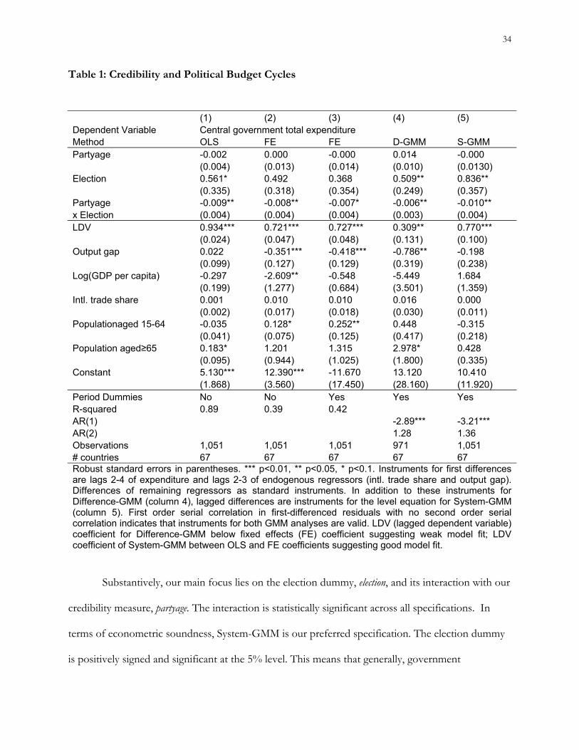
We begin our analysis by re-estimating Brender and Drazen’s base specification in Table 1,

substituting our first credibility measure, partyage. Across all models, political budget cycles are

significantly smaller in countries with older political parties. We first present the results of a ‘naïve’

Ordinary Least Squares (OLS) regression in column 1 and account for fixed effects in column 2,

including period dummies in column 3. Dynamic panel bias is evident in the divergent coefficient

estimates for the lagged dependent variable in the OLS and FE models, reinforcing the

appropriateness of GMM estimation.

Column (4) reports results from the Difference-GMM estimator, used by Brender and

Drazen. The coefficient of the lagged dependent variable (0.30) in column 4 is far below the

estimate with fixed effects (0.73) in column 3. This indicates that the Difference-GMM specification

in fact exhibits even higher bias than the FE model. System-GMM in column 5, on the other hand,

yields more credible results: the coefficient for the lagged dependent variable under System-GMM

lies in between the FE and OLS estimates, suggesting that it is a more appropriate specification.

34

Table 1: Credibility and Political Budget Cycles

(1) (2) (3) (4) (5) Dependent Variable Central government total expenditure Method OLS FE FE D-GMM S-GMM Partyage -0.002 0.000 -0.000 0.014 -0.000

(0.004) (0.013) (0.014) (0.010) (0.0130) Election 0.561* 0.492 0.368 0.509** 0.836**

(0.335) (0.318) (0.354) (0.249) (0.357) Partyage -0.009** -0.008** -0.007* -0.006** -0.010** x Election (0.004) (0.004) (0.004) (0.003) (0.004) LDV 0.934*** 0.721*** 0.727*** 0.309** 0.770***

(0.024) (0.047) (0.048) (0.131) (0.100) Output gap 0.022 -0.351*** -0.418*** -0.786** -0.198

(0.099) (0.127) (0.129) (0.319) (0.238) Log(GDP per capita) -0.297 -2.609** -0.548 -5.449 1.684

(0.199) (1.277) (0.684) (3.501) (1.359) Intl. trade share 0.001 0.010 0.010 0.016 0.000

(0.002) (0.017) (0.018) (0.030) (0.011) Populationaged 15-64 -0.035 0.128* 0.252** 0.448 -0.315

(0.041) (0.075) (0.125) (0.417) (0.218) Population aged≥65 0.183* 1.201 1.315 2.978* 0.428

(0.095) (0.944) (1.025) (1.800) (0.335) Constant 5.130*** 12.390*** -11.670 13.120 10.410

(1.868) (3.560) (17.450) (28.160) (11.920) Period Dummies No No Yes Yes Yes R-squared 0.89 0.39 0.42 AR(1) -2.89*** -3.21*** AR(2) 1.28 1.36 Observations 1,051 1,051 1,051 971 1,051 # countries 67 67 67 67 67 Robust standard errors in parentheses. *** p<0.01, ** p<0.05, * p<0.1. Instruments for first differences are lags 2-4 of expenditure and lags 2-3 of endogenous regressors (intl. trade share and output gap). Differences of remaining regressors as standard instruments. In addition to these instruments for Difference-GMM (column 4), lagged differences are instruments for the level equation for System-GMM (column 5). First order serial correlation in first-differenced residuals with no second order serial correlation indicates that instruments for both GMM analyses are valid. LDV (lagged dependent variable) coefficient for Difference-GMM below fixed effects (FE) coefficient suggesting weak model fit; LDV coefficient of System-GMM between OLS and FE coefficients suggesting good model fit.

Substantively, our main focus lies on the election dummy, election, and its interaction with our

credibility measure, partyage. The interaction is statistically significant across all specifications. In

terms of econometric soundness, System-GMM is our preferred specification. The election dummy

is positively signed and significant at the 5% level. This means that generally, government

35

expenditure increases in election years, as predicted by the theory of political budget cycles. The

interaction effect is negative and also significant at the 5% level. This means that the magnitude of

political budget cycles increases with the average age of parties, in other words credibility. This lends

strong support to our theory.

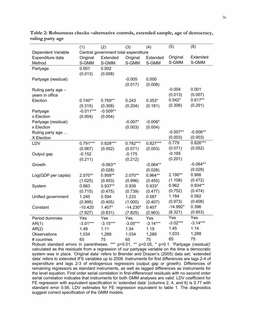
We test the robustness of this result in table 2. First, we include controls that we believe to

be more appropriate in this setting: we exclude the international trade share and the two age

dependency ratios and instead include controls for the political system and unified government.

Column 1 of table 2 shows that our results from table 1 are robust to this alternative specification.

In fact, the significance of the interaction effect increases slightly to 1 percent. In column 2, the

dependent variable is our extended data set. The dependent variable is the same as in Brender and

Drazen but now ranges up to 2008. The election dummy retains significance at the 5% level and the

interaction effect is correctly signed and significant at the 5 percent level.

Does party age just capture the effect of the age of the democratic system, as argued by

Brender and Drazen? To guard against this possibility, we replace our partyage variable with partyage

(resid), which is based on the residuals from a regression of partyage on the age of the democratic

system. The absolute size of the coefficients for both the election dummy and the interaction term

decrease slightly, both in the sample using Brender and Drazen’s original data in column 3 and our

data in column 4. However, the interaction effect retains significance at the 10% level, corroborating

our theory that it is credibility rather than whether a democracy is ‘new’ that determines the

magnitude of political budget cycles.

Lastly, we use our alternative measure of party consolidation, ruling party age – years in office.

We use this variable both in an analysis using the original Brender and Drazen data set in column 5

and our extended data in column 6. In both cases, the interaction effects with the election dummy

are positively signed, as expected, and significant at the 5% level.

36

Table 2: Robustness checks –alternative controls, extended sample, age of democracy, ruling party age

(1) (2) (3) (4) (5) (6)

Dependent Variable Central government total expenditure

Expenditure data Original Extended Original Extended Original Extended

Method S-GMM S-GMM S-GMM S-GMM S-GMM S-GMM

Partyage 0.001 0.002

(0.013) (0.008)

Partyage (residual) -0.005 0.000

(0.017) (0.008)

Ruling party age – -0.004 0.001

years in office (0.013) (0.007)

Election 0.740** 0.769** 0.243 0.353* 0.542* 0.617**

(0.315) (0.308) (0.204) (0.181) (0.306) (0.291)

Partyage -0.011*** -0.009**

x Election (0.004) (0.004)

Partyage (residual) -0.007* -0.006*

x Election (0.003) (0.004)

Ruling party age ... -0.007** -0.006**

X Election (0.003) (0.003)

LDV 0.791*** 0.828*** 0.782*** 0.827*** 0.779 0.826*** (0.067) (0.052) (0.071) (0.053) (0.071) (0.052)

Output gap -0.152 -0.175 -0.165

(0.211) (0.212) (0.201)

Growth -0.063** -0.064** -0.064**

(0.028) (0.028) (0.028)

Log(GDP per capita) 2.070** 0.958** 2.070** 0.964** 2.190** 0.966

(1.025) (0.453) (0.996) (0.455) (1.108) (0.472)

System 0.883 0.937** 0.939 0.933* 0.962 0.934**

(0.715) (0.475) (0.739) (0.477) (0.752) (0.474)

Unified government 1.240 0.594 1.233 0.587 1.184 0.582

(0.995) (0.405) (1.000) (0.407) (0.973) (0.408)

Constant -10.420 1.407* -14.230* 0.407 -14.992* 0.396

(7.827) (0.831) (7.825) (0.963) (8.321) (0.953)

Period dummies Yes Yes Yes Yes Yes Yes

AR(1) -3.01*** -3.15*** -3.05*** -3.14*** -3.02*** -3.14***

AR(2) 1.49 1.11 1.54 1.19 1.45 1.14

Observations 1,034 1,289 1,034 1,289 1,033 1,288

# countries 65 75 65 75 65 75 Robust standard errors in parentheses. *** p<0.01, ** p<0.05, * p<0.1. ‘Partyage (residual)’ calculated as the residuals from a regression of our partyage variable on the time a democratic system was in place. ‘Original data’ refers to Brender and Drazen’s (2005) data set; ‘extended data’ refers to extended IFS variables up to 2008. Instruments for first differences are lags 2-4 of expenditure and lags 2-3 of endogenous regressors (output gap or growth). Differences of remaining regressors as standard instruments, as well as lagged differences as instruments for the level equation. First order serial correlation in first-differenced residuals with no second order serial correlation indicates that instruments for both GMM analyses are valid. LDV coefficient for FE regression with equivalent specification in ‘extended data’ (columns 2, 4, and 6) is 0.77 with standard error 0.06. LDV estimates for FE regression equivalent to table 1. The diagnostics suggest correct specification of the GMM models.

37

In Table 3 we examine whether confidence in political parties also suppresses political

budget cycles. Since we are using a different dependent variable in this analysis, general government

final consumption expenditure, we also report the FE results: all GMM coefficients of the lagged

dependent variable lie above the FE coefficient, suggesting correct empirical specification.

Substantively, we find that, again, expenditure increases in election years, but less so the

more confidence voters have in parties. We employ different operationalisations of the election

dummy to check the robustness of this result. In columns 1 and 2, we employ the election dummy

based on Brender and Drazen’s coding rule of election years. The results are significant at the 5%

level for both the election dummy and the interaction with party confidence. In column 3, we code

elections as occurring in the previous year if held in the first month of the fiscal year. The absolute

size of the coefficients increases slightly but significance is unaltered. In column 4, we re-code

elections correspondingly if they occurred in the sixth month of the fiscal year – the results are

weakened but still significant at the 10% level. These results give us confidence that our results are

sensible, given different codings.

Finally, we repeat the test of table 2, and use our alternative party confidence measure,

purged of the effect of the age of the democratic system (party-confidence (resid)). The interaction with

the election dummy is positive, as predicted by our theory, and significant at the 5% level. This

shows that the effect of party confidence on the expenditure in election years is not driven by the

experience with democracy. This is reasonable as our main emphasis lies with parties, rather than

government per se. Overall, there is thus considerable evidence in support of our theory.

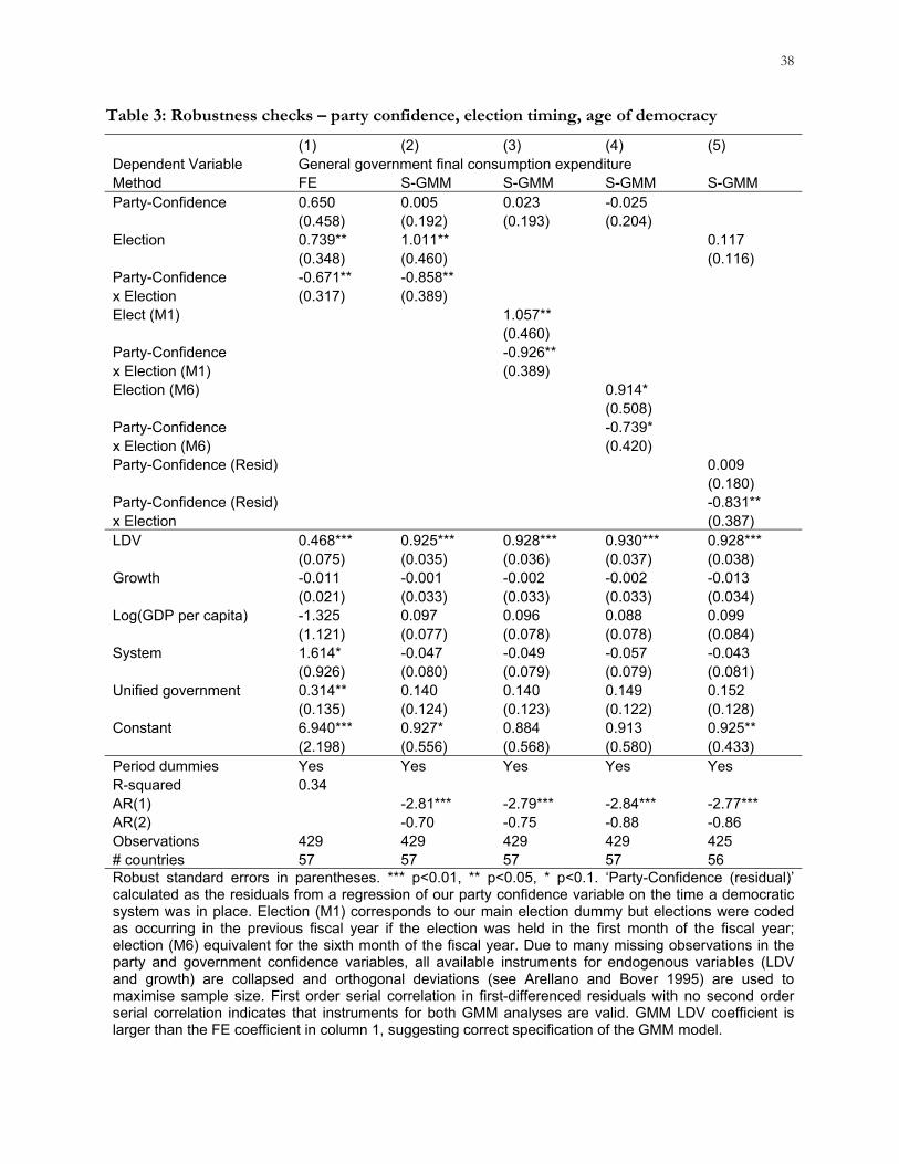
38

Table 3: Robustness checks – party confidence, election timing, age of democracy

(1) (2) (3) (4) (5) Dependent Variable General government final consumption expenditure Method FE S-GMM S-GMM S-GMM S-GMM Party-Confidence 0.650 0.005 0.023 -0.025

(0.458) (0.192) (0.193) (0.204) Election 0.739** 1.011** 0.117

(0.348) (0.460) (0.116) Party-Confidence -0.671** -0.858** x Election (0.317) (0.389) Elect (M1) 1.057**

(0.460) Party-Confidence -0.926** x Election (M1) (0.389) Election (M6) 0.914*

(0.508) Party-Confidence -0.739* x Election (M6) (0.420) Party-Confidence (Resid) 0.009

(0.180) Party-Confidence (Resid) -0.831** x Election (0.387) LDV 0.468*** 0.925*** 0.928*** 0.930*** 0.928***

(0.075) (0.035) (0.036) (0.037) (0.038) Growth -0.011 -0.001 -0.002 -0.002 -0.013

(0.021) (0.033) (0.033) (0.033) (0.034) Log(GDP per capita) -1.325 0.097 0.096 0.088 0.099

(1.121) (0.077) (0.078) (0.078) (0.084) System 1.614* -0.047 -0.049 -0.057 -0.043

(0.926) (0.080) (0.079) (0.079) (0.081) Unified government 0.314** 0.140 0.140 0.149 0.152

(0.135) (0.124) (0.123) (0.122) (0.128) Constant 6.940*** 0.927* 0.884 0.913 0.925**

(2.198) (0.556) (0.568) (0.580) (0.433) Period dummies Yes Yes Yes Yes Yes R-squared 0.34 AR(1) -2.81*** -2.79*** -2.84*** -2.77*** AR(2) -0.70 -0.75 -0.88 -0.86 Observations 429 429 429 429 425 # countries 57 57 57 57 56 Robust standard errors in parentheses. *** p<0.01, ** p<0.05, * p<0.1. ‘Party-Confidence (residual)’ calculated as the residuals from a regression of our party confidence variable on the time a democratic system was in place. Election (M1) corresponds to our main election dummy but elections were coded as occurring in the previous fiscal year if the election was held in the first month of the fiscal year; election (M6) equivalent for the sixth month of the fiscal year. Due to many missing observations in the party and government confidence variables, all available instruments for endogenous variables (LDV and growth) are collapsed and orthogonal deviations (see Arellano and Bover 1995) are used to maximise sample size. First order serial correlation in first-differenced residuals with no second order serial correlation indicates that instruments for both GMM analyses are valid. GMM LDV coefficient is larger than the FE coefficient in column 1, suggesting correct specification of the GMM model.

39

Conclusion

The inability of political actors to make credible commitments has been linked to increased

shirking and rent-seeking by politicians (Ferejohn 1984), clientelism (Keefer and Vlaicu 2008), and

significant differences in the policy choices of younger and older democracies (Keefer 2007). The

analysis here links the inability to make credible commitments to politician incentives to make

targeted transfers to voters prior to elections in order to mobilize electoral support. This same

theory offers a novel explanation of differences across countries in political budget cycles: less

credible politicians have greater incentives to shift expenditures to the period before elections. We

argue that institutionalized political parties, which facilitate collective action by citizens to punish

politicians who renege on their promises, are key to credibility. Accordingly, we use several

measures of party institutionalization to test the proposition that political budget cycles –

concentrated government expenditures around elections due to vote-buying – are greatest in

countries with weakly institutionalized parties.

The tests provide robust support for this proposition and for the underlying logic. First,

institutionalized political parties are essential for political credibility. Second, the absence of political

credibility encourages vote-buying. Third, differences in political incentives to undertake vote-

buying expenditures explain variations in political budget cycles. Our tests of these detailed

hypotheses are indirect and based on the reduced form examination of how expenditure cycles vary

with particular measures of political party institutionalization. The results point to a future research

agenda, which separately examines the structural links in the reduced form relationship and employs

more direct measures of political party organization.

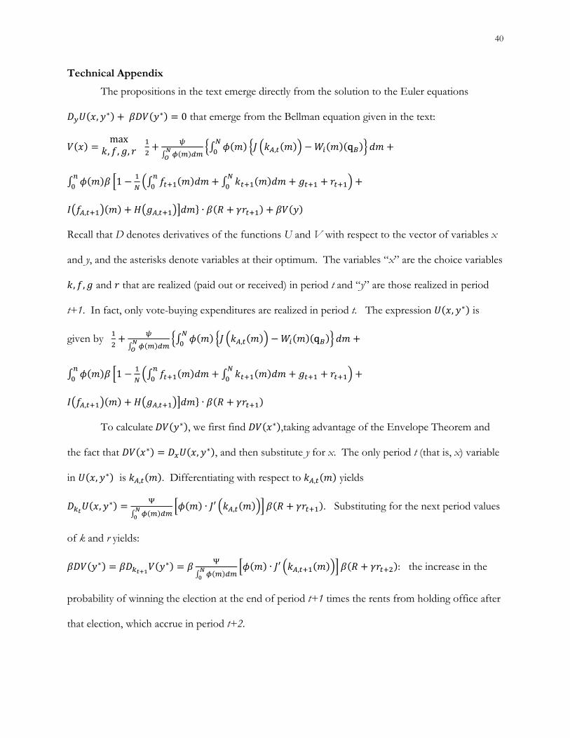
40

Technical Appendix

The propositions in the text emerge directly from the solution to the Euler equations

, ∗ ∗ 0 that emerge from the Bellman equation given in the text:

max, , , , q

1

, , ∙

Recall that D denotes derivatives of the functions U and V with respect to the vector of variables x

and y, and the asterisks denote variables at their optimum. The variables “x” are the choice variables

, , and that are realized (paid out or received) in period t and “y” are those realized in period

t+1. In fact, only vote-buying expenditures are realized in period t. The expression , ∗ is

given by , q

1

, , ∙

To calculate ∗ , we first find ∗ ,taking advantage of the Envelope Theorem and

the fact that ∗ , ∗ , and then substitute y for x. The only period t (that is, x) variable

in , ∗ is , . Differentiating with respect to , yields

, ∗ ∙ ′ , . Substituting for the next period values

of k and r yields:

∗ ∗ ∙ ′ , : the increase in the

probability of winning the election at the end of period t+1 times the rents from holding office after

that election, which accrue in period t+2.

41

Since none of the other choice variables appears in U, , ∗ , ∗

, ∗ 0. We therefore turn to the other term in the Euler equations, , ∗ , which is

calculated for each of the choice variables in y, , , , and .

Differentiating in turn yields:

, ∗ ∙ : holding constant what politicians

promise to do in period t+1for the voters who believe their promises, the more vote-buying of

group m that they undertake in period t+1 , the lower are their rents in period t+1.

, ∗ : Promises of

more public good spending increase the probability of election as long as the benefits of the public

good spending to the voters who believe politician promises outweigh the costs to those voters of

their share of the taxes needed to finance the public goods.

, ∗ ′ : Promises of greater

transfers to group m in period t+1 increase the probability of group m’s support, offset by the loss of

support from all the groups that believe politician promises and know their share of the taxes

needed to pay for the transfers.

, ∗ : the first term captures the fact

that higher rents in period t+1 crowds out spending that can be used to secure the support of voters

who believe politician promises, reducing expected rents; the second term reflects the fact that, in

equilibrium, candidate strategies are identical, q q , each has a 50 percent

chance of election, so an additional unit of rents earns, in expectation, for the candidate,

discounted by to account for the fact that rents are received in the next period.

The Euler conditions are then easily written.

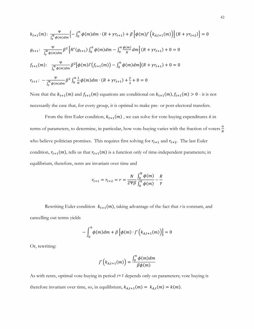
42

: ∙ ′ , 0

: 0 0

: ′ 0 0

: ∙ 0 0

Note that the and equations are conditional on , 0 - it is not

necessarily the case that, for every group, it is optimal to make pre- or post-electoral transfers.

From the first Euler condition, , we can solve for vote-buying expenditures k in

terms of parameters, to determine, in particular, how vote-buying varies with the fraction of voters

who believe politician promises. This requires first solving for and . The last Euler

condition, , tells us that is a function only of time-independent parameters; in

equilibrium, therefore, rents are invariant over time and

2Ψ

Rewriting Euler condition , taking advantage of the fact that r is constant, and

cancelling out terms yields

∙ ′ , 0

Or, rewriting:

′ ,

As with rents, optimal vote-buying in period t+1 depends only on parameters; vote buying is

therefore invariant over time, so, in equilibrium, , , .

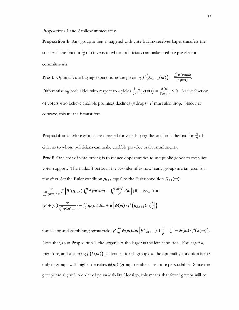
43

Propositions 1 and 2 follow immediately.

Proposition 1: Any group m that is targeted with vote-buying receives larger transfers the

smaller is the fraction of citizens to whom politicians can make credible pre-electoral

commitments.

Proof: Optimal vote-buying expenditures are given by ′ , .

Differentiating both sides with respect to n yields 0. As the fraction

of voters who believe credible promises declines (n drops), must also drop. Since is

concave, this means must rise.

Proposition 2: More groups are targeted for vote-buying the smaller is the fraction of

citizens to whom politicians can make credible pre-electoral commitments.

Proof: One cost of vote-buying is to reduce opportunities to use public goods to mobilize

voter support. The tradeoff between the two identifies how many groups are targeted for

transfers. Set the Euler condition equal to the Euler condition :

∙ ,

Cancelling and combining terms yields ∙ ′ .

Note that, as in Proposition 1, the larger is n, the larger is the left-hand side. For larger n,

therefore, and assuming ′ is identical for all groups m, the optimality condition is met

only in groups with higher densities (group members are more persuadable) Since the

groups are aligned in order of persuadability (density), this means that fewer groups will be

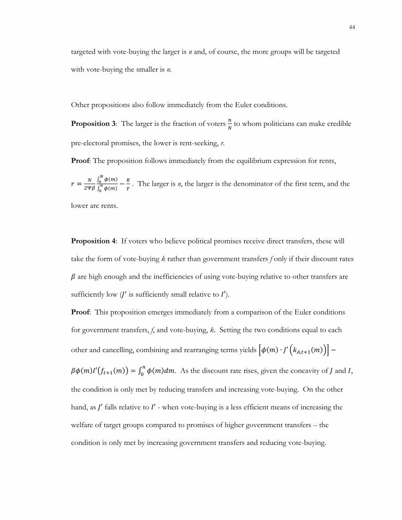
44

targeted with vote-buying the larger is n and, of course, the more groups will be targeted

with vote-buying the smaller is n.

Other propositions also follow immediately from the Euler conditions.

Proposition 3: The larger is the fraction of voters to whom politicians can make credible

pre-electoral promises, the lower is rent-seeking, r.

Proof: The proposition follows immediately from the equilibrium expression for rents,

. The larger is n, the larger is the denominator of the first term, and the

lower are rents.

Proposition 4: If voters who believe political promises receive direct transfers, these will

take the form of vote-buying k rather than government transfers f only if their discount rates

are high enough and the inefficiencies of using vote-buying relative to other transfers are

sufficiently low ( is sufficiently small relative to ′).

Proof: This proposition emerges immediately from a comparison of the Euler conditions

for government transfers, f, and vote-buying, k. Setting the two conditions equal to each

other and cancelling, combining and rearranging terms yields ∙ ′ ,

′ . As the discount rate rises, given the concavity of and ,

the condition is only met by reducing transfers and increasing vote-buying. On the other

hand, as ′ falls relative to ′ - when vote-buying is a less efficient means of increasing the

welfare of target groups compared to promises of higher government transfers – the

condition is only met by increasing government transfers and reducing vote-buying.

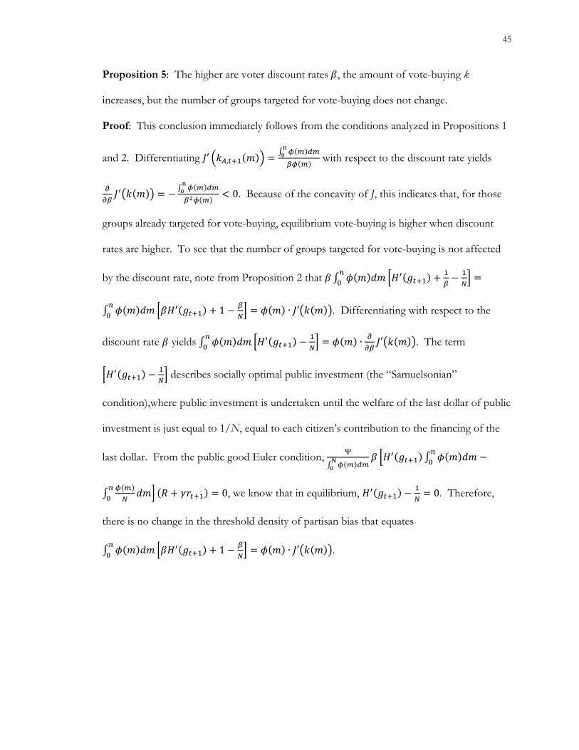
45

Proposition 5: The higher are voter discount rates , the amount of vote-buying k

increases, but the number of groups targeted for vote-buying does not change.

Proof: This conclusion immediately follows from the conditions analyzed in Propositions 1

and 2. Differentiating ′ , with respect to the discount rate yields

0. Because of the concavity of J, this indicates that, for those

groups already targeted for vote-buying, equilibrium vote-buying is higher when discount

rates are higher. To see that the number of groups targeted for vote-buying is not affected

by the discount rate, note from Proposition 2 that

1 ∙ ′ . Differentiating with respect to the

discount rate yields ∙ ′ . The term

describes socially optimal public investment (the “Samuelsonian”

condition),where public investment is undertaken until the welfare of the last dollar of public

investment is just equal to 1/N, equal to each citizen’s contribution to the financing of the

last dollar. From the public good Euler condition,

0, we know that in equilibrium, 0. Therefore,

there is no change in the threshold density of partisan bias that equates

1 ∙ ′ .

46

Appendix 1

Table A1: Re-coding of the election dummy

Country  Year  B&D  Adjusted 

Austria  1996  election  no election 

Ecuador  2000  election  no election 

Fiji  1994  no election  election 

India  1983  election  no election 

India  1984  no election  election 

Lithuania  1997  election  no election 

Lithuania  1998  no election  election 

Mauritius  1987  election  no election 

Mauritius  1988  no election  election 

Nepal  1997  election  no election 

Pakistan  1989  no election  election 

Papua New Guinea  1999  election  no election 

Peru  2000  no election  election 

Philippines  1995  election  no election 

South Africa  1994  no election  election 

South Africa  1995  election  no election 

South Africa  1999  no election  election 

South Africa  2000  election  no election 

Trinidad and Tobago  2001  no election  election 

Venezuela  1998  no election  election 

47

References

Acemoglu, Daron (2009). Introduction to Modern Economic Growth. Princeton: Princeton University

Press.

Acemoglu, Daron, Simon Johnson and James A. Robinson (2001). “The colonial origins of

comparative development: An empirical investigation.” American Economic Review 91:5, 1369-

401 (December).

Aldrich, John. (1995). Why parties? Chicago: Chicago University Press.

Alt, James E. and David Lassen (2006a). “Fiscal Transparency, Political Parties, and Debt in OECD

Countries” European Economic Review 50(6)1403-1436.

_____(2006b). “Transparency, Political Polarization, and Political Budget Cycles in OECD

Countries” American Journal of Political Science 50(3)430-550.

Alesina, Alberto, Arnaud Devleeschauwer, William Easterly, Sergio Kurlat and RomainWacziarg

(2002).“Fractionalization.” Journal of Economic Growth 8(2): 155-94 (June).

Arellano, Manuel and Olympia Bover (1995). “Another look at the instrumental variables estimation

of errorcomponentsmodels.” Journal of Econometrics 68: 29–51.

Beck, Thorsten, George Clarke, Alberto Groff, Philip Keefer, and Patrick Walsh (2001).“New Tools

in Comparative Political Economy: The Database of Political Institutions.” World Bank

Economic Review 15 (1): 165–76.

Block, Steven(2002). “Political Business Cycles, Democratization, and Economic Reform: The Case

of Africa” Journal of Development Economics 67:205-228.

Blundell, Richard and Stephen Bond(1998).“Initial conditions and moment restrictions in dynamic

panel data models.” Journal of Econometrics 87: 11–143.

Bond, Steven (2002). “Dynamic Panel Data Models: A Guide to Micro Data Methods and Practice”

Portuguese Economic Journal” 1:141-162.

48

Brender, Adi and Allan Drazen (2005). “Political budget cycles in new versus established

democracies.” Journal of Monetary Economics 52: 1271-1295.

_____ (2007). “Why is Economic Policy Different in New Democracies? Affecting Attitudes about

Democracy.”NBER Working Paper 13457.

_____ (2008). “How Do Budget Deficits and Economic Growth Affect Reelection Prospects?

Evidence from a Large Panel of Countries.”American Economic Review 98(5): 1271-1295.

Brusco, Valeria, Marcelo Nazareno and Susan C. Stokes (2004). “Vote Buying in Argentina.” Latin

American Research Review 39(2): 66-88

Callahan, William A. and Duncan McCargo (1996). “Vote-Buying in Thailand's Northeast: The July

1995 General Election.” Asian Survey 36(4 ): 376-392.

Cruz, Cesi and Philip Keefer (2012). “Programmatic Parties and the Politics of Bureaucratic

Reform.” Mimeo, The World Bank Development Development Research Group.

Dixit, Avinash and John Londregan (1996). “The Determinants of Success of Special Interests in

Redistributive Politics.” Journal of Politics 58 (4): 1132-55.

Drazen, Allan and Marcela Eslava (2008). “Electoral Manipulation via Voter-Friendly Spending:

Theory and Evidence.” Mimeo (July).

Gehlbach, Scott and Philip Keefer (2009). “Private Investment and the Institutionalization of

Collective Action in Autocracies: Ruling Parties, Militaries, and Bureaucracies.” Paper

presented at the 2009 meetings of the American Political Science Association.

Hansen, Lars P. (1982). “Large sample properties of generalised method of moments estimators.”

Econometrica 50: 1029–1054.

Holtz-Eakin, Douglas, Whitney Newey and Harvey Rosen (1988). "Estimating Vector

Autoregressions with Panel Data." Econometrica 56: 1371-1395.

Inglehart, Ronald (2004). World Values Surveys and European Values Surveys, 1999-2001. Ann

49

Arbor: MI: Inter-university Consortium for Political and Social Research.

Keefer, Philip (2011). “Collective Action, Political Parties and Pro-Development Public Policy.”

Asian Development Review (forthcoming).

_____ (2008).“Insurgency and credible commitment in autocracies and democracies.”World Bank

Economic Review. 22:1, 33-61.

_____ (2007).“Clientelism, credibility and the policy choices of young democracies.”American Journal

of Political Science 51:4, 804-821 (October).

_____ and RazvanVlaicu (2008). “Democracy, Credibility and Clientelism.”Journal of Law, Economics

and Organization 24:2, 371-406 (October).

Khemani, Stuti (2004). “Political cycles in a developing economy: effects of elections in the Indian

states.” Journal of Development Economics 73: 125-54.

Kitschelt, Herbert (2000). “Linkages between Citizens and Politicians in Democratic Polities.”

Comparative Political Studies 33 (6-7): 845-79.

Lindberg, Staffan I. (2003). “ ‘It’s Our Time to ‘Chop’: Do Elections in Africa Feed Neo-

Patrimonialism rather than Counteract it?” Democratization 10(2): 121-140.

Lohmann, Susanne. (1998). “Rationalizing the Political Business Cycle: A Workhorse Model”

Economics & Politics 10(1)1-17.

Nickell, Stephen J. (1981). “Biases in Dynamic Models with Fixed Effects.” Econometrica 49:6:1417-

1426.

Nichter, Simeon (2008). “Vote Buying or Turnout Buying? Machine Politics and the Secret Ballot.”

American Political Science Review 102 (1): 19 – 31.

Ockey, James (1994). "Political Parties, Factions and Corruption in Thailand." Modern Asian Studies

28(2): 251-77.

Persson, Torsten and Guido Tabellini (1990). Macroeconomic Policy, Credibility and Politics. London:

50

Harwood Academic Publishers.

Robinson, James A. and Ragnar Torvik (2005). “White Elephants.” Journal of Public Economics 89 (2-

3): 197-210.

Rogoff, Kenneth and Anne Sibert (1988). “Elections and Macroeconomic Policy Cycles.” The Review

of Economic Studies 55:1:1-16.

Rogoff, Kenneth (1990). “Equilibrium political budget cycles.”American Economic Review 80: 21-36.

Samuels, David J. (2002). “Pork Barreling Is Not Credit Claiming or Advertising: Campaign Finance

and the Sources of the Personal Vote in Brazil.” The Journal of Politics 64(3): 845-863.

Saporiti, Alejandro and Streb, Jorge M. (2008). “Separation of Powers and Political Budget Cycles.”

Public Choice 137(1):329-345.

Sargan, J. Denis (1958). “The estimation of economic relationships using instrumental variables.”

Econometrica 26:393-415.

Shi, Min and Jakob Svensson (2003).“Political Budget Cycles: A Review of Recent Developments.”

Nordic Journal of Political Economy 29(1): 67–76.

_____ (2006). “Political budget cycles: Do they differ across countries and why?” Journal of Public

Economics 90: 1367-1389.

Stokes, Susan C. (2005). “Perverse Accountability: A Formal Model of Machine Politics with

Evidence from Argentina.” American Political Science Review 99 (August): 315–25.

Wang, Chin-Shou and Charles Kurzman (2007). “Dilemmas of Electoral Clientelism: Taiwan,

1993.” International Political Science Review 28 (2): 225-245 (March).

Wurfel, David (1963). “The Philippines.” The Journal of Politics 25(4): 757-773.