Projective Visual Hulls

Svetlana Lazebnik1 (slazebni@uiuc.edu)Yasutaka Furukawa1 (yfurukaw@uiuc.edu)Jean Ponce1,2 (jponce@uiuc.edu)1 Department of Computer Science and Beckman InstituteUniversity Of Illinois, Urbana, IL 61801, USA2 Departement d’InformatiqueEcole Normale Superieure, Paris, France

Abstract. This article presents a novel method for computing the visual hull of a solidbounded by a smooth surface and observed by a finite set of cameras. The visual hullis the intersection of the visual cones formed by back-projecting the silhouettes foundin the corresponding images. We characterize its surface as a generalized polyhedronwhose faces are visual cone patches; edges are intersection curves between two viewingcones; and vertices are frontier points where the intersection of two cones is singular, orintersection points where triples of cones meet. We use the mathematical frameworkof oriented projective differential geometry to develop an image-based algorithm forcomputing the visual hull. This algorithm works in a weakly calibrated setting—thatis, it only requires projective camera matrices or, equivalently, fundamental matricesfor each pair of cameras. The promise of the proposed algorithm is demonstrated withexperiments on several challenging data sets and a comparison to another state-of-the-art method.

Keywords: Silhouette, visual hull, frontier point, projective differential geometry, oriented projectivegeometry, projective reconstruction, 3D photography.

1. Introduction

This article addresses the problem of computing the visual hull of a solid object

bounded by a smooth closed surface and observed by a finite number of pinhole

cameras. The visual hull is defined as the maximal volume consistent with an

object’s silhouettes as seen from some set of viewpoints (Laurentini, 1994), and

can be obtained by intersecting the solid visual cones formed by back-projecting

the object’s silhouettes found in each camera’s image plane (Figure 1). The idea

of approximating an object’s shape as an intersection of visual cones has existed

for over three decades, dating back to Baumgart (1974), and it continues to

be widely used today as a basis for many approaches to 3D photography, or

2

the acquisition of high-quality geometric and photometric models of complex

real-world objects — see (Hernandez Esteban and Schmitt, 2004; Furukawa and

Ponce, 2006; Matusik et al., 2002; Sinha and Pollefeys, 2005; Vogiatzis et al.,

2005) for a few recent examples. However, despite the computer vision com-

munity’s long-standing familiarity with the concept of the visual hull, the issue

of computing its intrinsic combinatorial and topological structure has received

relatively little attention. Most existing visual cone intersection algorithms pro-

duce generic volumetric or polygonal representations of their output, whereas

we argue in this article that the visual hull is much more naturally described

as a generalized polyhedron (Hoffmann, 1989) whose faces are patches belonging

to surfaces of individual visual cones, edges are segments of intersection curves

of pairs of cone surfaces, and vertices are isolated points of contact of three or

more faces. Equivalently, the boundary of the visual hull can be described as a

union of cone strips belonging to the surfaces of individual cones (Figure 2).

This article presents an algorithm for computing the boundary of the visual

hull by taking advantage of its intrinsically projective structure determined by

special kinds of contacts between visual rays and the object’s surface in 3D. (It

is well known that such contacts are the domain of projective geometry, and are

preserved under all smooth transformations that map lines to lines.) In particu-

lar, as we will show in Section 4, the vertices of the visual hull are of two types,

corresponding to two different types of contacts. The first vertex type, illustrated

in Figure 3(a), is a frontier point where visual rays from two different cameras are

simultaneously tangent to the object’s surface. A frontier point is a singularity

of an intersection curve between two cones where the two corresponding strips

cross each other (Figure 2). The second vertex type, illustrated in Figure 3(b),

is an intersection point where visual rays from three different cameras meet in

space after touching the surface of the object at three different locations. As seen

in Figure 2, three cone strips meet at each intersection point.

3

O

Apparent contour(outline)

Visual cone

Silhouette

Rim

Figure 1. A solid object Ω is observed by a camera with center O. The visual cone due to this camerais formed by back-projecting the silhouette of Ω seen in the camera’s image plane. The boundary ofthe silhouette in the image is the apparent contour or the outline γ. Note that γ is oriented such thatthe silhouette is on its left side (Section 3.2). The surface of the visual cone grazes the object along acurve called the rim.

Even though purely projective properties are sufficient to characterize the

vertices of the visual hull, they are insufficient to obtain a complete combinatorial

description of the visual hull boundary. In standard projective geometry, it is

impossible to define a half-line or a segment, and intuitive relations such as

front or back have no meaning. In the present article, we overcome this diffi-

culty by adopting an oriented extension of projective geometry (Stolfi, 1991).

More specifically, we follow the framework of oriented projective differential

geometry (Lazebnik, 2002; Lazebnik and Ponce, 2005), which gives us the most

elementary mathematical machinery sufficient for computing the visual hull. In

particular, it does not require cameras to be strongly calibrated and works when

only the fundamental matrices between pairs of cameras are known. Our method

is completely image-based, i.e., it does not perform any 3D computations such

as intersections of polyhedra in space. Unlike most existing approaches, ours

4

O1

O2O3

Figure 2. Toy example of visual hull construction. Three cameras with centers O1, O2, and O3 areobserving a spherical object. The three visual cones formed by back-projecting the silhouettes grazethe surface of the object along the three dashed rims. The visual hull surface is made up of three conestrips, indicated by three different shades (white corresponds to the first cone strip, dark gray to thesecond one, and light gray to the third one). As will be discussed in Section 4, vertices of the visualhull are of two types: frontier points (shown as black diamonds) where two strips cross each other,and intersection points (shown as white circles) where three strips meet. Note that frontier points alsocorrespond to pairwise intersections of rims — an important geometric fact that will be discussed indetail in Section 4.1.

produces a representation of the visual hull in terms of its intrinsic projective fea-

tures (i.e., frontier points, intersection points, and intersection curve segments),

instead of artifacts of discretization like polygons, voxels, or irregularly sampled

points.

The rest of the article is organized as follows. Section 2 discusses related

work, and Section 3 lists the key mathematical machinery and notation used

in our presentation. Section 4 describes the proposed algorithm for visual hull

construction. Along the way, we state several theoretical results (Propositions

5

Oj

i

j

Oi

X

Oi

Oj

i

j

Ok

k

X

(a) Frontier point (b) Intersection point

Figure 3. Two types of visual hull vertices. (a) X is a frontier point: The visual rays connecting cameracenters Oi and Oj to the surface point X lie in the tangent plane Π to the surface at this point. Notethat X lies on the intersection of rims Γi and Γj . (b) X is an intersection point: The three visual raysemanating from Oi, Oj , and Ok graze the surface at three distinct points (indicated in gray) on therespective rims Γi, Γj and Γk, and then meet in space at X.

1-3) establishing oriented constraints used at various stages of the algorithm.

To keep the presentation self-contained, we give abbreviated proofs of these

results in Appendix D. Section 5 describes practical details of our implementation

and Section 6 demonstrates results on several challenging real-world datasets

and presents a comparison with another state-of-the-art visual hull construction

algorithm (Franco and Boyer, 2003). Finally, Section 7 concludes with a summary

of our contributions and a discussion of our target application of 3D photography.

2. Related Work

One major branch of visual hull study is theoretical, focusing on characterizing

the shape that is consistent with the silhouettes of the target object observed

from every possible viewpoint. Significantly, even in this case the visual hull

cannot always exactly reproduce the object, since “dents” or concave parts

of the surface will never appear on its silhouettes. There exist algorithms for

computing the “limit” visual hull of polyhedral and smooth objects, in 2D and

in 3D (Laurentini, 1994; Petitjean, 1998; Bottino and Laurentini, 2004) but they

6

assume that a 3D geometric model of the target object is available. In this article,

we consider instead the more practical task of computing the visual hull of an

unknown object observed from a finite number of known viewpoints.

Historically, the main strategy for computing the visual hull has been to

directly implement the intersection of visual cones in 3D. The main advantage of

volume intersection algorithms is that they (in principle) work with any combina-

tion of calibrated input viewpoints and make no assumptions about the object

shape, e.g., smoothness or topology. The oldest such algorithm dates back to

Baumgart’s PhD thesis (1974), where a polyhedral visual hull is constructed by

intersecting the viewing cones associated with polygonal approximations to the

extracted silhouettes. A major disadvantage of such algorithms is that general

3D polyhedral intersections are relatively inefficient for the special-case problem

of intersecting visual cones, and can suffer from numerical instabilities. An alter-

native technique for visual hull construction is to approximate visual cones by

voxel volumes (Martin and Aggarwal, 1983; Potmesil, 1987; Ahuja and Veenstra,

1989; Srivastava and Ahuja, 1990; Szeliski, 1993). Voxel carving is not susceptible

to numerical difficulties that can arise in exact computations with polyhedra.

Moreover, its running time depends only on the number of input cameras and on

the resolution of the volumetric representation, not on the intrinsic complexity of

the visual hull. Parallel implementations of voxel carving can even achieve real-

time performance for such applications as 3D action reconstruction (Matsuyama

et al., 2004). On the other hand, volumetric visual hulls tend to suffer from

quantization artifacts, and require an extra step, e.g., the marching cubes algo-

rithm (Lorensen and Cline, 1987), to be converted to standard polygonal models.

Moreover, voxel-based models do not retain any information about the intrinsic

structure of the visual hull, i.e., locations of intersection curves and different cone

strips — information that is required by our subsequent approach to high-fidelity

high-resolution image-based modeling (Furukawa and Ponce, 2006).

7

Recent advances in image-based rendering and multi-view geometry have re-

sulted in new efficient algorithms that avoid general 3D intersections by taking

advantage of epipolar geometry. Matusik et. al. (2000) describe a fast, simple

algorithm that involves image-based sampling along visual rays emanating from

a virtual camera. The main limitation of this algorithm is that its output is

view-dependent: If one wishes to render the visual hull from a new virtual

viewpoint, one must re-run the construction algorithm. Another disadvantage

is that image-based visual hulls require custom-built rendering routines. Subse-

quent work (Boyer and Franco, 2003; Franco and Boyer, 2003; Matusik et al.,

2001; Shlyakhter et al., 2001) extends the idea behind image-based visual hulls to

produce view-independent polyhedral models. The most important contribution

of these newer algorithms is the reduction of 3D polyhedral intersections to 2D

— a strategy that will also be followed in this article.

In practical applications, one is often interested in reconstructing an object

from a video clip taken by a camera following a continuous trajectory. How-

ever, volume intersection techniques are ill-adapted to this task, which involves

handling large numbers of almost coincident visual cones. In this case, assum-

ing that the object is smooth, differential techniques of shape from deforming

contours (Cipolla and Giblin, 2000) become more appropriate. The foundation

for these techniques is given by mathematical relationships between the contour

generator or rim where the visual cone is tangent to the object and its projection

in the image plane, known as the apparent contour or outline (recall Figure 1).

One of the most basic facts is that observing a smooth point on the apparent

contour in the image is sufficient to reconstruct the tangent plane to the object

in space. If the camera moves continuously, the rim gradually “slips” along the

surface, and the surface may be reconstructed as the envelope of its tangent

planes. This is volume intersection in an infinitesimal sense, and the shape

obtained as a result of such an algorithm is also a visual hull. This approach

8

typically requires that the target objects be smooth, and precludes self-occlusion

or changing topology of evolving contours.

Koenderink (1984) was the first to elucidate the relationship between the

local geometry of the 3D surface and the geometry of the 2D contour in a single

image. Giblin and Weiss (1987) have introduced a reconstruction algorithm for

three-dimensional objects assuming orthographic projection and camera motion

along a great circle. Subsequent approaches have generalized this framework to

handle perspective projection and general (known) camera motions (Arbogast

and Mohr, 1991; Cipolla and Blake, 1992; Vaillant and Faugeras, 1992; Boyer

and Berger, 1997). All these approaches make extensive use of differential ge-

ometry, and focus on estimating local properties of the surface, such as depth

and Gaussian curvature — computations that require approximating first- and

second-order derivatives of image measurements and thus tend to be sensitive to

noise and computation error. Our approach also assumes smooth surfaces and

uses techniques of differential geometry to establish local properties of visual

hulls. However, our reconstruction algorithm does not rely on approximations of

local surface shape or curvature — the entity we compute is exactly the visual

hull. In addition, unlike infinitesimal methods, ours does not make restrictive

assumptions concerning self-occlusion or topology changes of the image contours.

The visual hull construction method presented in this article is based on

ideas introduced in (Lazebnik et al., 2001; Lazebnik, 2002). These ideas have

also served as a basis for an efficient algorithm to compute an exact polyhedral

visual hull (Franco and Boyer, 2003), and a hybrid algorithm combining voxel

carving and surface-based computation (Boyer and Franco, 2003). Other recent

developments include visual hull construction from uncalibrated images (Sinha

and Pollefeys, 2004), as well as Bayesian (Grauman et al., 2003; Grauman et al.,

2004) and algebraic dual-space approaches to visual hull reconstruction (Brand

et al., 2004). To our knowledge, our method remains the only one that computes

9

an exact image-based combinatorial representation of the visual hull while relying

solely on oriented projective constraints.

3. Mathematical Preliminaries

Before we start the discussion of our visual hull construction algorithm in Section

4, let us briefly introduce the mathematical machinery used in the rest of our

presentation. This machinery consists of basics of oriented projective geometry

(Section 3.1) and oriented representations of cameras and apparent contours

(Section 3.2).

3.1. Oriented Projective Geometry

In this presentation, we model the 2D camera plane and the ambient 3D space, as

oriented projective spaces T2 and T

3, respectively. By analogy with the standard

projective spaces P2 and P

3, which are formed by identifying all vectors of R3 and

R4 that are nonzero multiples of each other, T

2 and T3 are formed by identifying

all vectors of R3 and R

4 that are positive multiples of each other (Stolfi, 1991).

Note that according to its definition, the oriented plane T2 is topologically

equivalent to a 2-sphere, so in effect, we will be dealing with omnidirectional

cameras. Uppercase letters will denote flats (points, lines, and planes) in T3,

and lowercase letters will denote flats in T2. In the sequel, we will assume fixed

(but arbitrary) coordinate systems for all spaces of interest, and identify all flats

with their homogeneous coordinate vectors, which in the oriented setting are

unique up to a positive scale factor.

A line is spanned by two distinct points, i.e., a proper 2-simplex, and a plane

is spanned by three non-collinear points, i.e., a proper 3-simplex. Two simplices

spanning the same flat are said to have the same orientation when they are

related by an orientation-preserving transformation represented by a matrix with

a positive determinant. All the simplices of a given flat form two classes under

10

y

xz

l

l ∨ z = x ∨ y ∨ z = |x, y, z| > 0

Figure 4. Relative orientation of a line and a point in 2D. The counterclockwise arrow indicatesthe positive orientation of the 2D universe.

this equivalence relation, and an oriented flat is a flat to which an orientation has

been assigned by choosing one of these two classes as “positive.” To obtain the

simplex spanning the join of two flats, we simply concatenate the simplices that

span the two respective flats in that order. For example, in Figure 4 the join of

two points x and y is the oriented line l. This operation is denoted as l = x∨y, and

the homogeneous coordinate vector of l is given by the cross-product x× y. The

join of three points x, y, and z spans either the positive or the negative universe

of T2. The homogeneous (Plucker) coordinate of the universe is a scalar, and it is

given by the 3× 3 determinant |x, y, z|. Assuming that right-handed triangles in

T2 have been chosen as the positive ones, a necessary and sufficient condition for

x, y, and z to span the positive universe is |x, y, z| > 0 (when |x, y, z| = 0 then

the three points are collinear, and do not span the universe at all). Equivalently,

we can express the universe as the join of the line l = x ∨ y and the point z.

The sign of l ∨ z = lT z determines the relative orientation of l and z. Whenever

l ∨ z > 0 (resp. l ∨ z < 0), we will say that z lies on the positive (resp. negative)

side of l.

11

3.2. Cameras and Contours

Let us suppose that we are observing some solid Ω using n perspective cam-

eras.1 The solid is bounded by a smooth surface whose shape is to be inferred

based on the silhouette boundaries or outlines γ1, . . . , γn observed in the image

planes of the cameras. Let us assume that each outline possesses a regular

parametrization u → x(u) =(x1(u), x2(u), x3(u)

)Tsuch that the derivative

point2 x′(u) =(x′

1(u), x′2(u), x′

3(u))T

is not identically zero nor a scalar multiple

of x(u). This condition ensures that the tangent line t(u), formed by the join

x(u)∨x′(u) of the outline point x(u) and its derivative point x′(u), is everywhere

well defined.3 We assume that the outline is naturally oriented in the direction

of increasing parameter values, and require this orientation to be such that the

image of the interior of Ω is always located on the positive (left) side of the

outline (refer back to Figure 1 for an illustration of this convention). Provided

that this orientation convention is met, the silhouettes are allowed to have holes

and multiple connected components.

In addition to the outlines, our algorithm requires as input an estimate of

the epipolar geometry of the scene, consisting of fundamental matrices Fij and

epipoles eij between each pair of cameras. The issue of finding properly ori-

ented fundamental matrices and epipoles has been addressed in several pub-

lications (Werner and Pajdla, 2001a; Werner and Pajdla, 2001b; Chum et al.,

2003). In practice, however, one usually does not compute the epipolar geometry

between each pair of cameras from scratch. Instead, it is more convenient to

compute the fundamental matrices based on properly oriented projective esti-1 For the sake of our implementation, we assume that the object is inside the viewing volume of

each camera. Unlike some voxel-based methods, we do not deal with the issue of partial observation.2 In homogeneous coordinates, the successive derivatives x(i)(u) represent points in T

2 (by contrast,when a non-homogeneous coordinate representation is used, as in the Euclidean case, derivatives arethought of as vectors instead of points).

3 Note that the smoothness assumption is violated at a small number of isolated contour locationscorresponding to T-junctions. However, in the implementation we ignore T-junctions and assume thatthe contour is everywhere smooth. This introduces only a small amount of approximation error to the“true” silhouettes, and does not affect the procedure for visual hull computation, since the visual hullis well defined as the intersection of the visual cones formed by back-projecting the objects’ silhouettesregardless of whether the contours bounding the silhouettes are non-smooth or contain T-junctions.

12

mates of the camera matrices P1, . . . ,Pn. To be more specific, to ensure proper

orientations of the camera projection matrices, we must enforce the constraint

that any point xi observed in the image plane of the ith camera is equal up

to a positive scale factor to the computed projection PiX, denoted xi PiX.

These sign consistency constraints can either be built into the projective bundle

adjustment procedure or imposed a posteriori using the simple “sign flipping”

technique described in Hartley (1998).4 Assuming that all camera matrices have

thus been assigned consistent orientations, fundamental matrices and epipoles

can be computed using the properly oriented formulas given in Appendix A.

4. Computing the Visual Hull

This section develops our method for computing the visual hull using only ori-

ented projective constraints. A high-level summary of the proposed algorithm is

given in Figure 5. The visual hull is constructed in two stages: First, we find the

1-skeleton, i.e., the set of all vertices and edges of the visual hull; and second,

we “fill in” the interiors of the cone strips.

The first stage is implemented as an incremental algorithm that, at the end of

the ith iteration, produces the complete 1-skeleton of the intersection of visual

cones numbered 1 through i. To add the (i + 1)st visual cone, the existing

1-skeleton is modified in two steps: First, all parts of the existing 1-skeleton

that fall outside the new cone (and thus cannot belong to the visual hull by

definition) are clipped away; and second, intersection curves of the (i+1)st cone

with all previous cones are traced and clipped against all pre-existing views.

After processing all n cones in this fashion, we have a complete combinatorial

representation of the boundaries of all n cone strips composing the visual hull

surface, but we do not yet have an explicit representation of the strips themselves.

4 Since we restrict ourselves to the oriented projective setting where the cameras are in effectspherical, we do not have to deal with the more troublesome cheirality or visibility constraints thatarise when computing Euclidean upgrades. See Nister (2004) for a recent treatment of this issue.

13

To obtain such a representation, we triangulate the strips using a sweepline

algorithm.

Note that our incremental algorithm is not “optimal” from the viewpoint of

computational efficiency, since the results of many of its intermediate computa-

tions do not contribute to the final visual hull. However, it has the advantage

of being very simple, and, as shown in Section 6.3, can outperform a non-

incremental algorithm. It must also be noted that an incremental strategy can

be preferable in certain practical situations. For example, it can be used with

an experimental setup in which input images are acquired sequentially. Instead

of waiting until all images of the object have been taken, it may be preferable

to build an intermediate model based on the available data. Moreover, in such

a system, the user could halt the computation as soon as the model achieves an

acceptable degree of approximation to the target object.

The next three sections will describe the details of the algorithm’s three key

subroutines: tracing intersection curves between pairs of visual cones (Section

4.1); clipping interesection curves (Section 4.2); and triangulating the cone strips

(Section 4.3).

4.1. Tracing an Intersection Curve

Let us consider the cones associated with cameras i and j, whose surfaces are

formed by back-projecting the outlines γi and γj, parametrized by u and v,

respectively. Their intersection curve, denoted Iij, consists of 3D points X for

which there exists a choice of parameters u and v such that the rays formed by

back-projecting the outline points xi(u) and xj(v) intersect. This is expressed by

the well-known epipolar constraint

f(u, v) = xj(v)TFijxi(u) = 0 , (1)

where Fij is the fundamental matrix between views i and j. Note that (1) can

be seen as an implicit equation of a curve δij in the joint parameter space of γi

14

Input: Outlines γ1, . . . , γn, fundamental matrices Fij .Output: A combinatorial representation of the visual hull boundary.

[Find the 1-skeleton.]For i = 2, . . . , n

Clip each existing edge of the 1-skeleton against γi.For j = 1, . . . , i − 1

Trace the intersection curve Iij .For k = 1, . . . , i − 1, k = j

Clip each edge of Iij against γk.End For

End ForEnd For

[Find the visual hull faces.]For i = 1, . . . , n

Triangulate the ith cone strip.End For

Figure 5. Overview of the visual hull construction algorithm.

and γj.5 Thus, instead of directly tracing the intersection curve Iij in 3D, we can

trace δij in the (u, v)-space. This strategy has been inspired by an algorithm for

finding the intersection of two ruled surfaces published in the computer-aided

design community (Heo et al., 1999).

Note. In the oriented setting, the epipolar constraint f(u, v) = 0 is actually

not a sufficient condition for the corresponding visual rays to intersect in space.

That is, given two points xi(u) and xj(v) that satisfy (1), there does not always

exist a physical 3D point X such that xi(u) PiX and xj(v) PjX . Appendix

B (Proposition 4) gives the additional epipolar consistency condition needed

to guarantee the existence of X , and describes a simple way to eliminate the

connected components of δij that do not meet this condition. In our subsequent

presentation, we will use δij to denote only the set of consistent components of

the curve implicitly defined by f(u, v) = 0.

5 Since we allow silhouettes to have holes and multiple connected components, the outlines consistof one or more disjoint simple loops, and the parameter space has the topology of a collection of oneor more tori.

15

4.1.1. Critical Points of an Intersection Curve

Our general strategy for tracing δij is as follows: We break up the implicitly

defined curve into branches where one variable (say, v) can be expressed as

a function of the other (u) and then trace each branch separately, recording

along the way the global information about connectivity of the branches. This

subsection will treat the first step towards implementing this strategy, namely,

specifying the critical points along which the curve is to be broken up, and

characterizing the local behavior of δij in the neighborhood of each of these

points.

Let fu and fv denote partial derivatives of f with respect to u and v. Then

the derivative of v with respect to u, given by dvdu

= −fu

fv, is undefined wherever

fv = 0. At any such point, v cannot be locally expressed as a function of u.

Thus, we define points where fv = 0 as critical. To preserve symmetry between

the variables u and v, we also expand the definition to points where fu = 0.

Then all critical points (u0, v0) of of δij can be classified into the following three

types:

1. fu(u0, v0) = 0, fv(u0, v0) = 0;

2. fu(u0, v0) = 0, fv(u0, v0) = 0;

3. fu(u0, v0) = 0, fv(u0, v0) = 0.

To understand the geometric significance of these types, let us begin by

computing the derivatives fu and fv:

fu = xTj Fijx

′i = x ′

iTFjixj = x ′

i ∨ lij = |xi, x′i , eij| , (2)

fv = x ′jTFijxi = x ′

j ∨ lji = |xj, x′j, eji| . (3)

When fu = 0, xi is distinguished by the geometric property that its tangent line

ti = xi ∨ x′i passes through the epipole eij, or equivalently, that the derivative

point x′i lies on the epipolar line lij = eij∨xi (Figure 6). When fv = 0, the point xj

in the jth view is analogously characterized by epipolar tangency. Of particular

16

X

xixj

Oi

lij lji

Oj

eij eji

i j

i j

Figure 6. Frontier point (see text).

interest is the case of simultaneous epipolar tangency, when fu = 0 and fv = 0.

Then xi and xj are projections of a frontier point X that is the intersection of the

rims Γi and Γj on the surface (Rieger, 1986; Porrill and Pollard, 1991; Cipolla

et al., 1995). The surface tangent plane at X coincides with the (unoriented)

epipolar plane defined by Oi, Oj and X. The epipolar plane also coincides with

the tangent planes of the ith and jth visual cones at X, and the direction of

the intersection curve, which is normally given by the line of intersection of the

cones’ tangent planes, is locally undefined. Therefore, a frontier point gives rise

to a singularity of the intersection curve.

In accordance with the above analysis, if a critical point (u0, v0) is of type 1,

then xi(u0) and xj(v0) are images of a frontier point visible in both views (Figure

7, top); if it is of type 2, xi(u0) is an epipolar tangency in the ith view and xj(v0)

is a transversal intersection of the epipolar line lji = Fijxi(u0) with the outline

γj (Figure 7, middle); and if it is of type 3, xj(v0) is an epipolar tangency in the

jth view and xi(u0) is a transversal intersection of lij = Fjixj(v0) with γi (Figure

7, bottom). In the joint parameter space, critical points of type 1 correspond

to singularities of δij, while critical points of types 2 and 3 correspond to local

extrema in v- and u-directions, respectively. Using second-order techniques for

analyzing singularities of an intersection curve of two implicit surfaces (Hoff-

17

Type 1j

lji

i

lijxi 0( )u xj 0( )v

image i image j

v0

ij

u0

( , ) spaceu v

Type 2j

lji

i

lijxi 0( )u xj 0( )v

image i image j

v0

ij

u0

( , ) spaceu v

Type 3j

lji

i

lijxi 0( )u xj 0( )v

image i image j

v0

ij

u0

( , ) spaceu v

Figure 7. Critical point types (see text).

mann, 1989; Owen and Rockwood, 1987), it is straightforward to determine the

geometry of δij in the neighborhood of a singularity:

Proposition 1. Let (u0, v0) be a point on δij such that fu(u0, v0) = 0 and

fv(u0, v0) = 0. Then δij in the neighborhood of (u0, v0) has an X-shaped crossing,

that is, it consists of two transversally intersecting curve branches with tangent

vectors given by (a, 1) and (−a, 1), where a =√− fvv

fuu.

The proof of the above proposition is given in Appendix D.1. Note that instead

of thinking of a singularity as an X-shaped crossing, we can think of it as a vertex

with four incident branches. The tangent vectors pointing along each of these

branches are (a, 1), (−a, 1), (a,−1) and (−a,−1). Each of these vectors points

into a different “quadrant” obtained by partitioning a neighborhood of (u0, v0)

with the lines u = u0 and v = v0. Consequently, we can uniquely identify each

of the four branches by the sign label of the quadrant it locally occupies, i.e.,

++, +−, −+, −− (Figure 8, left). In order to assign analogous sign labels to

18

branches incident on critical points of type 2 and 3, we first have to determine

whether these critical points are local maxima or minima in the direction of u

and v, respectively. The next proposition, which is proved in Appendix D.2, tells

us how to make this determination, resulting in the complete classification of

critical point types shown in Figure 8.

Type 1 Type 2A Type 2B Type 3A Type 3Bfu = 0, fv = 0 fu = 0, fv = 0 fu = 0, fv = 0 fu = 0, fv = 0 fu = 0, fv = 0

local min local max local min local max

Figure 8. A complete classification of critical points with sign labels of incident branches. The figureshows sign labels for the branches incident on each critical point. The first (resp. second) sign iden-tifies whether the value of u (resp. v) increases or decreases as we follow a particular branch awayfrom (u0, v0) (note that by construction, a branch of the curve must be monotone, i.e., uniformlynondecreasing or nonincreasing, with respect to both the u- and the v-axis).

Proposition 2. Consider the points xi = xi(u0) and xj = xj(v0) on γi and γj

such that that (u0, v0) is a type 2 critical point of δij. Consider the derivatives

fv |xj, x′j, eji| tj ∨ eji and

fuu = x′′i ∨ lij

|xi, x′i, x

′′i | , if ti lij

−|xi, x′i, x

′′i | , if ti −lij .

(4)

Then (u0, v0) is a local maximum (resp. minimum) in the v-direction if the signs

of fv and fuu are the same (resp. opposite).

Analogously, if (u0, v0) is a type 3 critical point of δij, then it is a local maxi-

mum (resp. minimum) in the u-direction if the signs of fu and fvv are the same

(resp. opposite).

Let us consider the geometric meaning of the sign of fuu. Based on Eq. (4),

we can see that this sign depends on two factors: first, whether the epipolar

line lij coincides with the tangent line ti to γi at xi or whether the two lines

have opposite orientations; and second, whether the quantity κi = |xi, x′i, x

′′i | is

19

positive or negative. Significantly, κi is an oriented projective invariant that tells

us about the local shape of γi at xi: if κi is positive (resp. negative), then γi is

convex (resp. concave) in the neighborhood of xi (Lazebnik and Ponce, 2005).

Thus, we can see that the characterization of critical point types, which is a

crucial prerequisite for the intersection curve tracing algorithm presented in the

next section, depends on elementary local geometric properties of contours, their

tangents, and epipolar lines.

We can obtain an alternative interpretation of fuu by thinking of the task of

searching for all frontier points in the ith view as finding the zeros of fu = ti∨eij.

Since the geometric interpretation of the sign of fu is the relative orientation of

the tangent line ti and the epipole eij, and since fuu is the first derivative of this

function, the sign of fuu at a point when fu = 0 tells us whether this relative

orientation is changing from negative to positive or vice versa. When fuu > 0,

the tangent line is turning in such a way that the epipole begins to appear

on its positive side; the situation is reversed for fuu < 0. We will make use of

this interpretation in Section 5.1 when defining frontier point classifications for

discretely sampled contours.

4.1.2. The Tracing Algorithm

Given the characterization of critical points derived in the previous section, it

is now straightforward to develop an algorithm for tracing δij. The algorithm

begins by finding all critical points of the intersection curve and determining

their types using the test of Proposition 2. Each critical point, depending on

its type, serves as the origin of at most two branches leading in the increasing

direction of u, i.e., having sign labels ++ or +−. As can be seen from Figure 8,

critical points of types 1 and 3A have both ++ and +− branches, those of type

2A have one ++ branch, those of type 2B have one +− branch, and those of

type 3B have none. Accordingly, the algorithm uniquely identifies each branch

of the intersection curve by noting its origin and sign label (++ or +−), and

proceeds to trace the branch away from its origin, stopping when the second

20

endpoint is detected. The steps of finding critical points and tracing individual

branches are explained in more detail below.

Critical points are found as follows: For each epipolar tangency in the ith view,

i.e., a contour point xi(u) such that |xi, x′i , eij| = 0, we draw the corresponding

epipolar line lji = Fij xi in the jth view and find all intersections of this line

with γj. For each point of intersection xj(v), we add the pair of parameter values

(u, v) to the list of critical points. In this way, all the critical points of type 2 are

identified. To find all critical points of type 3, we carry out the same procedure

with the roles of the ith and jth views interchanged. Extra care is required to

correctly identify critical points of type 1 that occur whenever xi(u) and xj(v)

are epipolar tangencies lying along exactly matching epipolar lines. However, in

practice this situation never occurs: Because of (unavoidable) errors in contour

extraction and/or camera calibration, whenever we have an epipolar tangency

in one image, the corresponding epipolar line in the other image either misses

the contour entirely, or intersects it in a pair of nearby points. Thus, instead of

a singularity or a critical point of type 1, we observe a pair of critical points

of type 2 or 3 (Figure 9). This also affects the local topology of the visual hull

surface: instead of two cone strips that cross each other at the singularity, as in

the ideal case depicted in Figure 2, one strip becomes interrupted or “covered”

by the other one.

Each intersection curve branch is traced as follows: At each step, a fixed

increment is added to the current value of u, and the corresponding value of v is

found by locally searching along γj for the nearest intersection with the epipolar

line lji(u) = Fijxi(u). More precisely, let (ut−1, vt−1) be the point of the branch

found in the previous iteration of the tracing procedure, and let ut be the next

value of u. Then the corresponding vt is the parameter value of the outline point

nearest to xj(vt−1) where lji(ut) intersects γj (Figure 10, left). Note that we

search for vt in the increasing (resp. decreasing) direction of v if the sign label

of the current branch is ++ (resp. +−). The trace terminates when either γi or

21

Type 2j

lji

i

lijxi 0( )u

xj 1( )v

image i image j

v1

ij

u0

( , ) spaceu v

v2

xj 2( )v

Type 3j

lji

i

lij xi 1( )u

image i image j

ij

u1

( , ) spaceu v

v0

xj 0( )vxi 2( )u

u2

Figure 9. Top: The contour γj has been “perturbed” so that the epipolar line lji intersects γj in twopoints xj(v1) and xj(v2). As a result, δij loses the crossing and acquires two critical points of type 2.Bottom: An analogous perturbation of γi results in a pair of type 3 critical points.

j

lji( )ut1

i

xi t1( )u xj t( )v 1

image i image j

xi t( )u xj t( )vlji( )ut

j

lji( )ut1 xj ( )vt1

image (branch terminates)j

xj t( )vlji( )ut

Figure 10. The incremental process for tracing an intersection curve (see text). The white points onthe right part of the figure show two epipolar tangencies of γj in the interval [vt−1, vt], indicating thatthe trace of the current branch needs to terminate.

γj contains epipolar tangencies in the interval [ut−1, ut] or [vt−1, vt] (Figure 10,

right) and the critical point first encountered is recorded as the second vertex

of the current branch. For completeness, we must also consider the situation

when the intersection curve has no critical points at all. This can happen, for

example, when the target object is convex and the line connecting the camera

centers Oi and Oj passes through its interior, so that the epipoles fall inside the

silhouettes in both views and neither outline has epipolar tangencies. In such

a case, we simply pick an arbitrary starting point u0 to begin the tracing and

continue until the current value of u reaches u0 again.

22

(a) (b)

(c) (d)

Figure 11. (a), (b) Two views with outlines and epipolar lines corresponding to critical points. Theepipolar lines tangent to the outlines are solid, and the epipolar lines corresponding to frontier pointsin the other view are dashed. Note that (a) and (b) show the gourd from opposite sides, so thatthe leftmost epipolar line in (a) corresponds to the rightmost epipolar line in (b) and so on. (c) Theintersection curve δij . The horizontal axis is u and the vertical axis is v. Critical points of types 2A,2B, 3A, and 3B are indicated by , , , and , respectively. (d) The intersection curve in 3D.

Figure 11 illustrates the output of the intersection curve tracing algorithm

using an example of two views of a gourd. As part (d) of the figure shows, we

can easily obtain a 3D representation of Iij (in a projective coordinate system, of

course) by triangulating the pairs of contour points xi(u) and xj(v) corresponding

to each (u, v) in δij. A particularly simple linear triangulation method (Forsyth

and Ponce, 2002) is as follows. Let X be the (unknown) coordinate vector of a

23

point on Iij, and let xi(u) PiX and xj(v) PjX be its projections on the ith

and jth contours. Then we can write the projection constraints asxi × PiX = 0 ,xj × PjX = 0 .

This is a system of six linear homogeneous equations in four unknowns whose

least-squares solution gives us an estimate of X (note that there is a sign ambi-

guity in this estimate; it can be resolved by enforcing the orientation consistency

of the original projection constraints).

4.2. Finding the 1-skeleton

Next, we move on to the second step of computing the visual hull: finding its

1-skeleton, or the subset of its boundary comprised of segments of intersection

curves between pairs of input views. When the visual hull is formed by inter-

secting only two cones, the 1-skeleton is simply the intersection curve between

the two cones. With more than two cameras present in the scene, the task of

computing the 1-skeleton becomes more complicated: We must determine which

fragments of the(

n2

)different intersection curves actually belong to the visual

hull, and then establish the connectivity of these fragments.

First, let us discuss how to compute the contribution of a given intersection

curve Iij to the 1-skeleton. Recall that the visual hull consists of points whose

images do not fall outside the silhouette of the object in any input view. We

enforce this property by projecting Iij into each available view k = i, j and

“clipping away” the parts that fall outside the silhouette in the kth view. Let ιkij

denote the projection of Iij into the kth view. This projection can be obtained

either from a 3D representation of Iij, or directly from δij via an image-based

transfer operation (see Appendix C for a brief treatment of oriented epipolar

transfer). Following reprojection, we compute the subset of the curve ιkij that

also lies inside the kth silhouette (Figure 12). This operation involves “cutting”

ιkij along points where it intersects γk. As will be explained in Section 5.2, these

points can be found efficiently with the help of a few simple data structures.

24

(a) (b)

(c) (d)

Figure 12. Clipping the intersection curve of Figure 11 against a third view of the gourd. (a) Thereprojected intersection curve superimposed upon the third image. (b) The intersection curve clippedagainst the silhouette. (c) The clipped curve in 3D. (d) The complete 1-skeleton for nine views.

Consider a point xk that simultaneously lies on γk and on ιkij. It is easy to

see (Figure 13) that xk is the projection of an intersection point X in 3D that

simultaneously belongs to the ith, jth, and kth visual cones. X can also be

described as a trinocular stereo match of points on the three respective outlines,

though in a generic situation, it is not a true physical point on the surface of the

object being reconstructed.6 Since X is the point of incidence of three segments

6 For the intersection point to lie on the surface, the trifocal plane would have to be tangent to theobject, which does not happen when the cameras are in general position.

25

xi

xk

xj

X

OjOi

Ok

Iij

Iik

Ijk

ikjk

ij

i j

k

i

j

k

Figure 13. X is an intersection point between views i, j, and k. The thick black curves incident onX are fragments of Ijk, Iik, and Iij that belong to the 1-skeleton of the visual hull. The parts of therespective intersection curves that are “clipped away” by the ith, jth, and kth cones are dashed. Theobject Ω is not shown to avoid clutter.

belonging to the pairwise intersection curves Iij, Ijk, and Iik, it is found three

times in the course of our procedure for computing the 1-skeleton: when clip-

ping Ijk against the ith silhouette, when clipping Iik against the jth silhouette,

and when clipping Iij against the kth silhouette. Therefore, after carrying out

all the clipping operations, we must complete the combinatorial description of

the 1-skeleton by joining the triple occurrences of each intersection point and

recording the incidence of the corresponding intersection curve segments. Our

implementation of the joining procedure will be discussed in Section 5.3.

26

4.3. Triangulation of Cone Strips

The complete boundary of the visual hull consists of strips lying on the surfaces

of the original visual cones (Figure 14). The 1-skeleton obtained at the end of the

clipping stage gives us a complete combinatorial representation of all the strip

boundaries, consisting of vertices that are critical points and intersection points,

and edges that are segments of intersection curves. However, we do not yet have

an explicit description of the strip interiors. To obtain such a description in the

form of meshes suitable for rendering and visualization, we must triangulate the

cone strips. Our triangulation algorithm is given in Figure 15. In the rest of

this section, we give a high-level explanation of this algorithm, and in Section

4.3.1, we fill in the technical details necessary to its implementation, namely, the

definitions of linear ordering and front/back status of strip edges.

The ith cone strip may be thought of as a collection of intervals along the

continuous family of visual rays Li(u), each of which is formed by back-projecting

the corresponding point xi(u) on γi. Accordingly, we perform triangulation by

sweeping the visual ray Li(u) along the strip in the increasing direction of the

contour parameter u. We can think of this operation as a 2D vertical line sweep

standard in computational geometry if we imagine “cutting” the cone strip along

Figure 14. The visual hull of the gourd computed from nine views (top left) and the nine constituentcone strips.

27

Input: Cone strip.Output: A triangulation of the cone strip.

Create event list by sorting the parameter values of the endpoints of all edgeson the boundary of the cone strip. Initialize the active list with all edges thatcontain some starting position u0.

For each event ut

[Fill in triangles from ut−1 to ut.]For each pair (E,E′) of adjacent edges in the active list such thatE is a front edge and E′ is a back edge

Fill in triangles between E and E′ in the interval [ut−1, ut].End For[Update the active edge list.]If ut is an event where an edge starts

Insert edge into active list.Else If ut is an event where an edge ends

Delete edge from the active list.End If

End For

Figure 15. Overview of the cone strip triangulation algorithm.

L u( )t1i L ui t( )

E1

E2

E3

E4

E5

E6

Figure 16. Triangulating a cone strip between two consecutive events ut−1 and ut. The two visualrays L(ut−1) and L(ut) are shown as parallel vertical lines. The active edge list consists of edgesE1, . . . , E6, in that order. Edges with odd (resp. even) indices are front (resp. back). At this stage,the algorithm triangulates the cells between edge pairs (E1, E2), (E3, E4), and (E5, E6).

28

some arbitrary parameter value u0 and “stretching” it on a plane so that the

visual rays turn into vertical lines and the contour parameter u increases from

left to right (Figure 16). In the horizontal direction, all edge points of the cone

strip are kept sorted by their u-coordinates. In the vertical direction, the edge

points are sorted according to an oriented projective linear ordering. The precise

definition of this ordering will be given in Section 4.3.1, but for now, we can

think of it as sorting all the points that intersect the same visual ray according

to their distance from the ith camera center (because of our commitment to the

oriented projective framework, we cannot use metric depth or distance values

directly).

The two key data structures maintained by the triangulation algorithm are an

event list and an active list. The event list gives the discrete set of u-coordinates

through which the sweeping ray passes in the course of the algorithm. These

coordinates, sorted in the increasing order of u, correspond to the endpoints of

all the strip edges. The active list, updated at each successive event value, is a

list of edges that intersect the sweeping ray at its current location. If the ray

passes the first endpoint of an edge, that edge is inserted into the active list,

and if the ray passes the second endpoint of an edge already in the list, that

edge is deleted. The edges in the active list are kept sorted according to their

linear order along the sweeping ray. In addition, they are also labeled by their

front/back status. This status, which will be formally defined in Section 4.3.1,

describes the relative location of the edges with respect to the strip interior.

Namely, between any two consecutive event locations ut−1 and ut, the boundary

of the cone strip decomposes into pairs of front/back edges that bound pieces of

the cone strip, or cells, in their interior. For example, in Figure 16, the interior of

the strip is bounded between edge pairs (E1, E2), (E3, E4), and (E5, E6). These

cells are monotone, i.e., they intersect the sweeping ray along at most a single

interval. They are triangulated using a simple linear-time algorithm for monotone

polygons (O’Rourke, 1998). This step is completely standard, and we omit its

29

details in our presentation. In practice, the triangles obtained by this procedure

are very long and thin, and require remeshing (see Section 5.4 for details).

4.3.1. Linear Ordering and Front/Back Status

In the remaining part of this section, we complete the specification of the trian-

gulation algorithm by supplying the definitions of linear ordering and front/back

status. We first define these notions for individual points where the sweeping ray

intersects a cone strip, and then extend them to entire edges of the cone strip.

Let X and Y be two distinct points on the visual ray Li. We can define a

linear ordering relation “<” on these points as follows:

X < Y iff Li X ∨ Y .

It is possible to compute this ordering in an image-based fashion by looking at

the projections of the points X and Y into some other view j. The visual ray

Li projects onto the epipolar line lji = Fijxi, while X and Y project onto points

xj = PjX and yj = PjY . The projection preserves the relative orientation of X

and Y , so we have

Li X ∨ Y iff lji xj ∨ yj . (5)

The notion of linear ordering can be easily extended from individual points

lying on a visual ray to two edges of a cone strip that are intersected by the

same visual ray. Let E and E ′ denote two edges of the ith cone strip and Li be

any ray touching these edges in two distinct points X and Y . Because of the way

we construct strip edges, E and E ′ cannot intersect in their interior (at most,

they can share an endpoint). Therefore, the relative ordering of X and Y will

remain the same for any ray Li that intersects both E and E ′, and we can say

that E < E ′ if and only if X < Y for some particular choice of the two points.

In order to insert a new edge into the active list, we must locate its proper

position with respect to the existing active edges. Since the active list is kept

sorted, we can locate the new edge using a binary search that involves a series of

comparisons against individual active edges. Let E denote an active edge, and

30

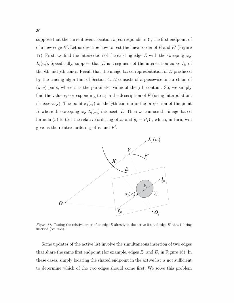
suppose that the current event location ut corresponds to Y , the first endpoint of

of a new edge E ′. Let us describe how to test the linear order of E and E ′ (Figure

17). First, we find the intersection of the existing edge E with the sweeping ray

Li(ut). Specifically, suppose that E is a segment of the intersection curve Iij of

the ith and jth cones. Recall that the image-based representation of E produced

by the tracing algorithm of Section 4.1.2 consists of a piecewise-linear chain of

(u, v) pairs, where v is the parameter value of the jth contour. So, we simply

find the value vt corresponding to ut in the description of E (using interpolation,

if necessary). The point xj(vt) on the jth contour is the projection of the point

X where the sweeping ray Li(ut) intersects E. Then we can use the image-based

formula (5) to test the relative ordering of xj and yj = PjY , which, in turn, will

give us the relative ordering of E and E ′.

Oi

X

Y

Oj

x ( )vj t

eji

j

Li t( )u

lji

yj

E

E'

Figure 17. Testing the relative order of an edge E already in the active list and edge E′ that is beinginserted (see text).

Some updates of the active list involve the simultaneous insertion of two edges

that share the same first endpoint (for example, edges E1 and E2 in Figure 16). In

these cases, simply locating the shared endpoint in the active list is not sufficient

to determine which of the two edges should come first. We solve this problem

31

by selecting a value of u that falls in the interior of both edges, constructing

the points where they meet the ray Li(u), and testing the relative orientation of

these two points.

Next, let us define the front/back classification of intersection curve points

bounding the cone strip. Let X be a point on the boundary of the ith cone strip,

and Li be the visual ray passing through X . X is said to be a front (resp. back)

point with respect to the ith view if it is the first (resp. last) point of the interval

on Li that lies on the visual hull and has X as an endpoint. That is, for any

point Y in the interior of this interval, we have X < Y (resp. X > Y ). The

following proposition, whose proof is given in Appendix D.3, yields a convenient

image-based criterion for determining the front/back status of X (Figure 18):

Proposition 3. Suppose that X is a point on the 1-skeleton of the visual hull

that belongs to the intersection curve Iij. Then X is a front (resp. back) point

on the boundary of the ith cone strip if and only if tj ∨ eji < 0 (resp. > 0), where

tj is the tangent to γj at the point xj = PjX .

Notice that the sign of tj ∨ eji can only change at a frontier point. Since

the edges of the 1-skeleton cannot contain frontier points in their interior, the

front/back status is actually the same for all points in the interior of a single

edge of the 1-skeleton. Thus, just as with linear ordering, we can extend the

definition of front/back status to apply to entire edges. Namely, an edge E of

the 1-skeleton, considered as part of the boundary of the ith cone strip, is called

front (resp. back) if each point in its interior is a front (resp. back) point.

In the course of the triangulation algorithm, we have to test the front/back

status of an edge when it is inserted into the active list. This is done by applying

the test of Proposition 3 to its first endpoint X, provided that X is not a type

3A critical point. In the latter case, the projection xj of X in the jth view

is a frontier point, and the test fails because tj ∨ eji = 0. In principle, it is

still possible to determine the front/back status of the edge using only local

information, based on the behavior of the first and second derivatives of the

32

Oi

X

Y

Oj

yj

eji

j

tj

Li

lji

xj

Figure 18. Front/back status of points on visual rays. X is a front point of the bold interval on theray Li because tj ∨ eji < 0 (the positive orientation of the image plane is counterclockwise). Y is aback point.

jth contour at xj (Lazebnik, 2002). We omit the details of this analysis in the

current presentation, since a more robust and straightforward solution to the

same problem is simply to test another point in the interior of the edge.

5. Implementation Details

We have implemented the proposed approach in C++. This section discusses

implementation issues that have not been addressed so far in this article.

5.1. Discrete Contour Representation

In describing our algorithms in Section 4, we have assumed a continuous con-

tour representation. In the implementation, however, contours are piecewise-

linear. Therefore, we now need to give discrete definitions of frontier points and

alternative formulas for computing their types.

33

A frontier point on a piecewise-linear contour is a vertex whose two incident

edges have different relative orientations with respect to the epipole. This def-

inition is illustrated in Figure 19, left, where xi is a vertex and t−i and t+i are

the two contour “tangents”—that is, the properly oriented lines containing the

two edges preceding and following xi along the contour orientation, respectively.

Then the necessary and sufficient condition for xi being a frontier point can be

written as

t−i ∨ eij −t+i ∨ eij .

Notice that we are making the general position assumption that the epipole

does not lie on either t−i or t+i . In practice, we have found this assumption to be

justified, since noise and errors in contour extraction and calibration effectively

“perturb” all the data points, thereby eliminating degeneracies.

lji

eij

xi xj

image i image j

ti

tieji

+

_

tj

lij

Figure 19. Discrete computation of critical points and their types (see text).

Next, we need to give a discrete analogue of Proposition 2, which is necessary

for determining critical point types during tracing of intersection curves. Since

we cannot directly compute the differential quantities fv and fuu used in this

proposition, we will fall back on their geometric interpretations. Recall that the

sign of fuu tells us about the change of the relative orientation of the contour

tangent and the epipole. Namely, when fuu > 0, the epipole migrates from the

negative to the positive side of the tangent, and when fuu < 0, it migrates

from the positive side to the negative. This reasoning directly translates to the

34

following discrete rule:

fuu > 0 ⇐⇒ t−i ∨ eij < 0 and t+i ∨ eij > 0 ,

fuu < 0 ⇐⇒ t−i ∨ eij > 0 and t+i ∨ eij < 0 .

For example, in Figure 19, fuu > 0 at xi. The other important quantity used in

Proposition 2 is fv = tj ∨ eji. It is also used in Proposition 3 to determine

the front/back status of a point of the 1-skeleton using purely image-based

information. To compute tj ∨ eji in the discrete case, we simply define tj as

the properly oriented line supporting the edge of the jth contour that contains

xj, the point of intersection of the contour and the epipolar line lji (Figure 19,

right). Note that by our general position assumption, xj cannot be a vertex. In

the figure, we have tj ∨ eji < 0 at xj.

5.2. Computational efficiency: Clipping intersection curves

Most of the processing time of our visual hull construction algorithm is spent

on two basic operations, curve/line and curve/curve intersections. These op-

erations are performed during tracing of intersection curves and clipping of

reprojected intersection curves against image contours, respectively. Recall from

Section 4.1.2 that most line-contour intersections performed by our algorithm are

incremental—that is, the line is moved by a small offset, and the new intersection

is found by searching in the neighborhood of the previous one. Effectively, this

approach finds each new intersection in constant time, so this operation is not

a major source of inefficiency for our algorithm. Thus, the main computational

bottleneck for our approach is clipping the projection ιkij of an intersection curve

Iij against an image contour γk. In the implementation, ιkij and γk are both

piecewise linear, and the clipping procedure reduces to a sequence of intersection

checks between each line segment of ιkij and the contour γk. Next, let us describe

the data structures that we use to perform these checks efficiently (Figure 20,

(a)-(c)). In order to make the implementation as simple as possible, we subdivide

35

ιkij to make sure that its every segment has length of at most one pixel in the

image.

The first data structure is a bitmap Bk, whose resolution is the same as that

of the kth input image. Bk(x, y) is set to 1 if γk passes through the corresponding

pixel, and 0 otherwise. Note that the bitmap contains 0 in most of the pixels.

Then, if a line segment covers only empty pixels, we can tell in time proportional

to the segment’s image length that there are no intersections. In our case, since

the length of all segments is bounded above by a pixel, this check effectively takes

constant time. The second data structure is an array of C bins Gck(c = 1, . . . , C),

where each bin stores a subset of the line segments forming the contour γk. More

concretely, suppose the height of the kth image is Yk, then the bin Gck stores

the set of line segments whose corresponding y-intervals intersect with the range

[Ykc−1C

, YkcC

]. Note that a single line segment can be stored in multiple bins.

For example, in Figure 20 (c), red, green, and blue line segments are stored

in G1k, G

2k, and G3

k, respectively. We let C = 15 throughout our experiments,

while for the purpose of illustration, C = 3 in Figure 20 (c). With the help of

the above two data structures, the intersection check between a line segment s

and the image contour γk is performed as follows: If Bk(x, y) = 0 for all the

pixels which s passes through, report no intersection (the fast check), otherwise

compute intersection(s) of s with all the line segments stored in the bins whose

corresponding y-intervals intersect with that of s (the slow check). Note that

since our implementation guarantees that s is less than one pixel in length,

there must exist at least one interval that fully contains s.

Let M and N denote the numbers of line segments in ιkij and γk, respectively,

and P denote the number of intersections between these curves. In theory, we

have P = O(MN). For typical datasets, however, it is reasonable to assume

that P is bounded above by a constant smaller than M and N . Furthermore,

most of the segments forming ιkij require only a constant-time fast check against

γk, while the number of segments that require slow checks is on the order of P .

36

Under these assumptions, since the worst-case cost of a slow check is linear in

N (and is in fact accelerated by a significant constant using our multi-bin data

structure), the running time of the algorithm is thus O(M + NP ). In practice,

this results in a significant improvement over the brute-force implementation

that exhaustively intersects each segment of ιkij with each segment of γk and

thus has complexity O(MN).

1

0γ

Gk

Gk

Gk

Yk

Bk(x,y)

1

2

3

k

Boundary edge

hole(a) (b)

(c)

(d)

Figure 20. Implementation details. Efficient implementation of the clipping procedure: (a) Given animage contour γk, we build two additional data structures: (b) A bitmap Bk(x, y), and (c) A set of binsGc

k storing line segments in γk (see text for details). (d) Due to failures in identifying triple intersectionpoints, our outputs may contain holes. To fill them, we first identify boundary edges where a face isdefined only on one side. Then, we trace the boundaries, identify loops, and triangulate them to fillholes.

5.3. Identifying intersection points

As explained in Section 4.2, every time a new image is added in our incremental

construction algorithm outlined in Figure 5, we obtain a set of triple intersection

points that need to be identified. Each point is associated with three images: the

pair of images used to generate an intersection curve and the third image used to

clip it. For each triple of images, we collect the corresponding intersection points,

and perform the following greedy identification procedure. Let X1, X2 and X3 be

three intersection points associated with images i, j, and k, with corresponding

37

contour parameter values (u1, v1, w1), (u2, v2, w2), and (u3, v3, w3). Then the cost

function for identifying this triple is

∑(l,m)∈(1,2), (1,3), (2,3)

|ul − um| + |vl − vm| + |wl − wm| .

Triples of intersection points are identified using the following greedy algorithm:

1. Collect all intersection points associated with the same triple of images.

2. Find the triple from this set with the minimum identification cost.

3. If the cost is less than a pre-determined threshold µ, identify the three

points, remove them from the set and go back to the second step; otherwise,

terminate the procedure.

We set µ to 0.05 times the average image contour length in all our experiments.

In the results presented in Section 6, not all triples of intersection points are

successfully identified. In fact, as shown by Table I in the next section, up to

6% of intersection points can be left unmatched. However, these mistakes of

the identification process are not due to our greedy matching procedure, but

to the fact that the positions of the intersection points are not always precisely

estimated during the clipping procedure because of numerical inaccuracies of

the transfer (reprojection) procedure. It is also important to point out that in

practice, unmatched intersection points cause only small inconsistencies in the

structure of the computed visual hull model, and are easily repaired using the

hole-filling algorithm described next.

5.4. Hole filling and remeshing

Due to failures in identifying triple intersection points, cone strips formed by the

intersection curves may not be closed and may miss some of their boundaries.

As a result, the output of the triangulation algorithm described in Figure 15

may contain holes where edges are missing. To fill those holes, we use a simple

boundary traversal algorithm (Figure 20(d)). Given a polygonal mesh, we first

38

identify its boundary edges, where a face is defined on only one side, then trace

boundary edges to identify a loop, and finally trianglulate the loop to fill the

hole. Although it is a very simple procedure, holes have been successfully filled

at all the boundary edges in all our experiments. See Section 6.3 for a discussion

of topological consistency of the output.

The final implementation issue is remeshing. Recall from Section 4.3 that the

mesh produced by our strip triangulation algorithm lacks vertices in the interiors

of cone strips, and its triangles tend to be rather long and thin. However, image-

based modeling approaches that use the visual hull mesh to initialize multiview

stereo optimization, e.g., (Furukawa and Ponce, 2006), typically require meshes

with more uniformly sampled vertices, and triangles that have a better aspect

ratio. To obtain a higher-quality mesh for subsequent processing, we can perform

an optional remeshing step consisting of a sequence of edge splits, collapses, and

swaps (see (Hoppe et al., 1993) for details of these operations). Briefly, edge

splitting is performed for edges that are too long, edge collapsing is performed for

edges that are too short, and edge swapping is performed to make sure that the

degree of each vertex is close to six, thus yielding a more regular triangulation.

This process is constrained to make sure that important visual hull structures are

preserved: Namely, edge swaps and collapses are not performed if the operation

involves an edge that belongs to an intersection curve, i.e., an edge on the

boundary of two cone strips. Note that we perform remeshing only when the

visual hull mesh is required as input for further processing. In particular, all the

running times and mesh sizes reported in the next section are not affected by

remeshing.

6. Experimental Results

This section demonstrates the effectiveness of our visual hull algorithm by pre-

senting results on several challenging datasets and conducting a comparative

39

skull: 24 images dinosaur: 24 images alien: 24 images

1900 × 1800 2000 × 1500 1600 × 1600

predator: 24 images roman: 48 images

1800 × 1700 3500 × 2300

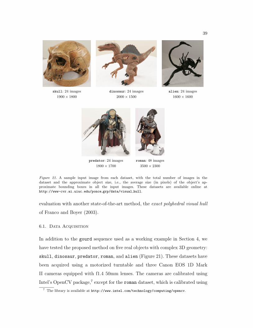
Figure 21. A sample input image from each dataset, with the total number of images in thedataset and the approximate object size, i.e., the average size (in pixels) of the object’s ap-proximate bounding boxes in all the input images. These datasets are available online athttp://www-cvr.ai.uiuc.edu/ponce grp/data/visual hull.

evaluation with another state-of-the-art method, the exact polyhedral visual hull

of Franco and Boyer (2003).

6.1. Data Acquisition

In addition to the gourd sequence used as a working example in Section 4, we

have tested the proposed method on five real objects with complex 3D geometry:

skull, dinosaur, predator, roman, and alien (Figure 21). These datasets have

been acquired using a motorized turntable and three Canon EOS 1D Mark

II cameras equipped with f1.4 50mm lenses. The cameras are calibrated using

Intel’s OpenCV package,7 except for the roman dataset, which is calibrated using

7 The library is available at http://www.intel.com/technology/computing/opencv.

40

Table I. Basic statistics of computed visual hull models. First three columns list the numbers ofcritical points, identified intersection points, and unidentified intersection points for each dataset.The fourth column lists the running time of our algorithm on an Intel Pentium IV desktop machinewith a 3.4GHz processor and 3GB of RAM. The first number is the time to build the 1-skeleton,and the second number is the time to triangulate cone strips and fill holes. The overall runningtime is the sum of the two.

Dataset# critical # identified # unidentified

time (s)pts. intersection pts. intersection pts.

skull 6,684 8,004 122 318.9 + 76.8

dinosaur 2,889 11,190 660 415.7 + 97.7

alien 1,168 9,052 602 478.6 + 53.7

predator 2,682 11,223 663 573.2 + 164.0

roman 10,840 32,319 1,697 4,051.3 + 1,154.3

the package of Lavest et al. (1998). It is important to note that, even though we

use strong calibration for convenience purposes, we do not actually rely on any

metric information in the process of computing the visual hulls.

We follow a semi-automatic procedure to extract outlines from the raw im-

ages. First, we manually segment foreground pixels using Adobe PhotoShop

and obtain discretized contours by traversing the boundary of the foreground

pixels. Next, we smooth the contours and resample them to make sure that

successive vertices are less than one pixel apart. Finally, we orient the contours

to observe the convention described in Section 3.2. In particular, this means

that the orientation of the holes is opposite of that of the outer contour. All

the datasets used in this section, including the original input images, camera

calibration parameters, and extracted contours, are publicly available at

http://www-cvr.ai.uiuc.edu/ponce grp/data/visual hull.

41

6.2. Computed Visual Hulls

This section presents results of our proposed visual hull computation algorithm

applied to the five objects from Figure 21. Figure 22 shows visual hull models

of each object from four different viewpoints. Table I gives basic statistics for

each model, including the numbers of critical points and identified/unidentified

intersection points generated during the procedure. Even though up to 6% of

intersection points are left unidentified, high-quality visual hull models are ob-

tained with the help of the hole-filling procedure described in Section 5.4. The

last two columns of Table I show the running times of the two stages of our

algorithm, namely, building the 1-skeleton and triangulating the cone strips.

Recall that our visual hull construction algorithm (Figure 5) is incremental,

i.e., it builds the visual hull by successively adding images one by one and

updating the model. Accordingly, Figure 23 illustrates how the visual hull is

refined as more input images are added. Finally, Figure 24 shows visual hull

models with textures from the original input images mapped onto their surfaces.

42

Figure 22. Computed visual hull models for each dataset as seen from four different viewpoints.

43

Figure 23. Incremental refinement of visual hull models. From left to right, subsets of 3, 4, 8, and 12images, respectively, are used to build the visual hull for each object.

44

Figure 24. Texture-mapped models. Each face (triangle) on the mesh is mapped with texture fromthe image whose corresponding optical axis has the smallest angle from the face normal orientation.This is obviously not a projective criterion, but we must emphasize that it is used for visualizationpurposes only, as texture-mapping is not part of the original visual hull construction algorithm.

6.3. Comparative Evaluation

This section presents a comparison between the method proposed in this arti-

cle and the exact polyhedral visual hull algorithm (EPVH) (Franco and Boyer,

2003; Franco, 2005). EPVH is a state-of-the-art recent algorithm that has been

explicitly designed to be robust and computationally efficient. The strategy em-

ployed by EPVH is, in a sense, complementary to ours: Whereas our algorithm

first computes the 1-skeleton and then fills in the interiors of the cone strips,

EPVH begins by computing the viewing edges, or intervals on visual rays that

lie in the interiors of the cone strips, and then fills in the intersection curve

segments and triple points that connect these edges. Unlike our algorithm, which

has to match triple occurrences of the same intersection points, EPVH finds each

intersection point exactly once. Finally, unlike our algorithm, which computes

45

many intermediate structures that do not belong to the final visual hull (i.e.,

subsets of intersection curves that later get clipped out), EPVH computes the

final visual hull surface in a non-incremental fashion.

Table II shows a comparison between our method and EPVH versions 1.0 and

1.1. These two versions have complexity O(n2 p2) and O(n2 p log p), respectively,

where n is the number of views and p is the average number of segments on each

image contour (Franco, 2005). Note that EPVH 1.1 has only become available

to us close to press time, and is more recent than our own implementation. To

make sure that the outputs and running times are exactly comparable, we have

used the same sets of piecewise-linear contours as inputs to all the algorithms.

The first two columns of Table II show the numbers of vertices (Nv) and faces

(Nf ) of the visual hull models computed by each method. We can see that

our models are somewhat larger in terms of the number of vertices and faces.

We have verified that the polygonal meshes constructed by all algorithms are

manifolds by checking two conditions: (1) Every edge is incident to exactly two

faces; and (2) the link of every vertex is a triagulation of the circle (Hoffmann,

1989). The meshes output by all algorithms satisfy these two conditions for all

the data sets. The third column of Table II shows the genus G of the models

computed using the Euler-Poincare formula (Hoffmann, 1989): Nv − Ne + Nf −2(1 − G) = 0, where Ne is the number of edges (not shown in the table).8

Note that the genera of the models produced by our method and EPVH are

different for most of the datasets. Even though the genus of the visual hull is often

different from that of the original object and the correct number is unknown,

our algorithm seems to produce extraneous small handles due to mistakes in

identifying triple intersection points and the subsequent hole-filling procedure.

By contrast, the models output by both versions of EPVH have fewer topological

imperfections because EPVH explicitly handles intersection points by iteratively

8 Note that the visual hulls for our data typically consist of multiple connected components, thelargest one containing the target object and several smaller ones not corresponding to any actualobject structure. Therefore, we discard these smaller components and compute all the numbers (Nv,Ne, Nf , G) only for the largest connected component.

46

generating missing points to remove inconsistencies (Franco and Boyer, 2003).

However, except for unmatched intersection points, which may cause microscopic

differences, the structure of the models produced by our method and EPVH looks

identical down to very small-scale detail, as shown in Figure 25.

Table II. Comparison of our method and two versions of EPVH. The numbers of vertices(Nv) and triangles (Nf ), and the genus of the largest connected component of the visualhull model are shown for our method and EPVH 1.0 and 1.1. The fourth column shows therunning times of all three algorithms, reported for an Intel Pentium IV desktop machine witha 3.4GHz processor and 3GB of RAM.

Dataset method # vertices # faces genus time (s)

ours 486,480 972,984 7 395.7

skull EPVH 1.0 401,832 803,684 6 5,614.4

EPVH 1.1 401,830 803,680 6 128.9

ours 337,828 675,664 3 513.4

dinosaur EPVH 1.0 290,452 580,900 0 6,329.5

EPVH 1.1 290,456 580,908 0 138.0

ours 209,885 419,770 1 532.3

alien EPVH 1.0 171,752 343,500 0 3,362.9

EPVH 1.1 171,752 343,500 0 119.3

ours 375,345 750,806 30 737.2

predator EPVH 1.0 306,152 612,420 30 5,078.2

EPVH 1.1 306,152 612,420 30 136.0

ours 1,258,346 2,516,764 19 5,205.6

roman EPVH 1.0 884,766 1,769,576 12 53,862.0

EPVH 1.1 884,750 1,769,544 12 2,147.4

The last column of Table II shows the running times of all three algorithms.

Note that our running time is the sum of the two numbers in the last column

of Table I. We can observe that our method runs from six to ten times faster

than EPVH 1.0, but two to five times slower than EPVH 1.1. A more complete

picture can be obtained by investigating how the performance of the different

methods scales with the size of the input. Accordingly, Figure 26 shows running

times for the three algorithms obtained by uniformly sampling image contours

at three different resolutions. Since our algorithm requires each contour segment

to be less than one pixel long, in addition to sub-sampling contour segments,

47

Ours EPVH 1.0 Ours EPVH 1.0

Figure 25. Detailed comparison of the visual hull models reconstructed by our method and EPVH1.0 (note that the outputs of EPVH 1.0 and 1.1 are exactly the same in most cases). First and secondcolumns: closeups of shaded models. Third and fourth columns: closeups of color-coded models, wherecone strips associated with different images are indicated by different colors.

we have multiplied their image coordinates by the sampling ratio. As Figure 26

shows, for every doubling of the contour resolution, the running time of EPVH

1.0 approximately quadruples, while the performance of our algorithm and of

EPVH 1.1 scales much better with input size. Unlike Franco and Boyer (Franco

and Boyer, 2003), we cannot give a simple expression for the asymptotic running

time of our algorithm since it depends in non-trivial ways on the geometric

complexity of the input object and of the silhouettes (for example, the time for

computing an intersection curve depends on the number of critical points, and

48

0.25 0.5 10

500

1000

1500

2000

2500

3000

3500

Sampling ratio

Run

ning

tim

e (s

ec)

Alien

EPVH 1.0oursEPVH 1.1

0.25 0.5 10

1000

2000

3000

4000

5000

6000

Sampling ratio

Run

ning

tim

e (s

ec)

Predator

EPVH 1.0oursEPVH 1.1

0.25 0.5 10

1

2

3

4

5

6x 10

4

Sampling ratio

Run

ning

tim

e (s

ec)

Roman

EPVH 1.0oursEPVH 1.1

Figure 26. Comparison of our method with EPVH 1.0 and 1.1 for three datasets (alien, predator,roman). The figure shows how the running times of the three algorithms change as we uniformlysub-sample the input image contours. Note that the complexity of the corresponding models (thenumbers of vertices and faces) scales approximately linearly for all methods, with EPVH 1.0 and 1.1producing smaller models than our algorithm, as can be seen from Table II.

the time for clipping this curve depends on the number of its intersections with

the silhouette). Nevertheless, based on our comparative evaluation of scaling

behavior, we conjecture that the asymptotic running time of our algorithm is

close to that of EPVH 1.1, but with larger constants to account for some ineffi-

ciencies in our current implementation. In particular, our algorithm spends time

on computations that are in principle unnecessary, such as computing parts of

intersection curves that are later clipped away. In the future, we plan to develop

an improved “hybrid” algorithm that would be like our current method in relying

exclusively on image-based oriented projective constructions, and like EPVH in

avoiding redundant computations and topological inconsistencies.

7. Discussion

This article has presented an image-based algorithm for computing visual hulls

using oriented projective constraints. The following is a summary of our main

contributions, both theoretical and practical:

− We characterize the surface of the visual hull in terms of its intrinsic pro-

jective features, i.e., frontier points, intersection curves, and intersection

points.

49

− We establish a connection between visual hull topology and multi-view ge-

ometry. Specifically, we show that frontier points and intersection points,

which determine the connectivity of cone strips, are in turn determined by

certain kinds of contacts between visual rays and the object’s surface (recall

Figures 2 and 3).

− We present a complete visual hull construction algorithm that utilizes only

oriented projective constraints (Lazebnik and Ponce, 2005; Stolfi, 1991).

In particular, this algorithm does not require strong calibration, only the

knowledge of fundamental matrices for all pairs of cameras in the scene.

− As part of our algorithm, we develop a novel procedure for tracing an in-

tersection curve between a pair of visual cones (Section 4.1.2) that relies on

an image-based classification of critical points (Proposition 2) derived from

local geometric properties of contours, their tangents, and epipolar lines.

− We demonstrate in Section 6 a practical implementation that works on chal-

lenging real-world data and has complexity comparable to that of another

state-of-the-art algorithm.

The key target application of our proposed algorithm is 3D photography, or

the acquisition of high-quality 3D models from photographs. In most cases,

the visual hull by itself is not a very good approximation to the target shape,

since it is required to conform only to the silhouettes in the original pictures.

A better approximation is given by a photo-consistent shape (Kutulakos and

Seitz, 1999) that must exactly reproduce the internal texture patterns seen in

the input images of the target object. Accordingly, Furukawa and Ponce (2006)

have used the visual hull construction algorithm proposed in this article to build

an initial approximation of the object that is subsequently refined using both

photo-consistency and silhouette-consistency constraints. Other 3D photography

approaches that use the visual hull for initialization include (Hernandez Esteban

50

and Schmitt, 2004; Sinha and Pollefeys, 2005; Sullivan and Ponce, 1998; Vogiatzis

et al., 2005).

Appendix

A. Oriented Epipolar Geometry

Let Pi and Pj be the properly oriented projection matrices of the ith and jth

cameras:

Pi =

P T

i

QTi

RTi

, Pj =

P Tj

QTj

RTj

.

The knowledge of these camera matrices enables us to compute the properly

oriented fundamental matrix Fij between each pair of views (Lazebnik, 2002):

Fij =

|Qi,Ri,Qj,Rj| |Ri,Pi,Qj,Rj| |Pi,Qi,Qj,Rj|

|Qi,Ri,Rj,Pj| |Ri,Pi,Rj,Pj| |Pi,Qi,Rj,Pj||Qi,Ri,Pj,Qj| |Ri,Pi,Pj,Qj| |Pi,Qi,Pj,Qj|

. (6)

The properly oriented expressions for the epipoles are as follows:

eij =

|Pi,Pj,Qj,Rj||Qi,Pj,Qj,Rj||Ri,Pj,Qj,Rj|

, eji =

|Pj,Pi,Qi,Ri||Qj,Pi,Qi,Ri||Rj,Pi,Qi,Ri|

.

B. Epipolar Consistency

If two points xi and xj are the projections of the same 3D point X , then the

epipolar constraint xTj Fijxi = 0 is satisfied. Let us now consider the converse

of this statement. For example, if we have xi PiX and xj −PjX , the

epipolar constraint is still satisfied, but there is no point in space with a well-

defined orientation that would project to the two image points. The following

proposition, equivalent to the “strong realizability” condition of Werner and

Pajdla (2001b), is proved in (Lazebnik, 2002):

51

Proposition 4. Let xi and xj be two points that satisfy the epipolar constraint

xTj Fijxi = 0 and do not coincide with the respective epipoles eij and eij. Then

there exists a 3D point X such that xi PiX and xj PjX if and only if

Fjixj eij ∨ xi or equivalently, Fijxi eji ∨ xj . (7)

Next, let us briefly discuss the implications of the epipolar consistency con-

straint for intersection curve tracing (Section 4.1). The expression (7) can be

written as a scalar inequality

g(u, v) > 0 , where g(u, v) =(Fijxi(u)

)·(eji ∨ xj(v)

). (8)

It is clear that g(u, v) is a smooth function. Moreover, if we assume that the out-

lines do not pass through the epipoles, g(u, v) never vanishes whenever f(u, v) =

xj(v)TFijxi(u) = 0. We must conclude that g(u, v) keeps the same sign within a

connected component of δij, and therefore, within any single branch delimited by

critical points. Thus, it is straightforward to identify the parts of δij that do not

correspond to physical components of the intersection curve in space: Namely, in

the first stage of tracing δij, when all its vertices (critical points) are identified,

it is sufficient to discard all vertices that fail the epipolar consistency test (8).

C. Oriented Epipolar Transfer

Suppose we know two points xi and xj in the ith and jth views that are the

projections of the same 3D point X . Without explicitly computing X itself, how

can we find the properly oriented point xk PkX in a third view? We can apply

the fundamental matrices Fik and Fjk to map the points xi and xj onto their

respective epipolar lines in the kth view, lki = Fikxi and lkj = Fjkxk, and then

take the intersection of these two lines (Figure 27). However, some extra work

needs to be done to ensure orientation consistency (refer to (Lazebnik, 2002) for

details). The properly oriented formula for xk is

xk = sgn((Fikxi) ∨ ekj

) ((Fjkxj) ∧ (Fikxi)

), (9)

52

xi

xk

xj

X

OjOi

Ok

ekiekj

lkilkj

Figure 27. Epipolar transfer (see text).

where the meet of the two lines Fjkxj and Fikxi is given by the cross-product

of their coordinate vectors. Though (9) is a simple and convenient formula, it

has some pitfalls. In particular, it fails whenever the 3D intersection point X

is located in the trifocal plane spanned by the camera centers Oi, Oj, and Ok.

In practice, the epipolar transfer relationship may become numerically unstable

whenever the intersection point lies near the trifocal plane. For this reason,

a better implementation choice may be to rely on the more robust transfer

procedure based on the trifocal tensor. Deriving this formula is beyond the scope

of this article, but refer to (Lazebnik, 2002) for details.

53

D. Proofs of Propositions 1-3

D.1. Proof of Proposition 1

We would like to find an explicit parametric form for δij in the neighborhood of

(u0, v0). This form is given by a curve(u(t), v(t)

)such that f

(u(t), v(t)

)≡ 0. As-

suming that u0 = u(t0) and v0 = v(t0), Taylor expansion of f(t) = f(u(t), v(t)

)about t0 yields

f(t0 + δt) = f(t0) + f ′(t0) δt +1

2f ′′(t0) δt2 + . . .

= f(u0, v0) + (fu u′ + fv v′) δt +

1

2

(fuu (u′)2 + 2fuv u′ v′ + fvv (v′)2 + fu u′′ + fv v′′) δt2 + . . .

=1

2

(fuu (u′)2 + 2fuv u′ v′ + fvv (v′)2

)δt2 + . . . . (10)

We obtained (10) by eliminating all terms involving the vanishing quantities

f(u0, v0), fu, and fv. We can further simplify (10) by noticing that the mixed

second derivative fuv = x ′jT Fijx

′i vanishes because the derivative points x ′

i and

x ′j lie on the respective matching epipolar lines lij = Fjixj and lji = Fijxi. The

Taylor expansion of f(t) now becomes

f(t0 + δt) =1

2

(fuu (u′)2 + fvv (v′)2

)δt2 + . . . .

To make sure that f(u(t), v(t)

)≡ 0, every coefficient of the Taylor series must

be identically zero. In order for the quantity fuu (u′)2 + fvv (v′)2 to vanish, we

must have

u′

v′ = ±√−fvv

fuu

.

Finally, by finding the expressions for fuu and fvv, it is straightforward to verify

that − fvv

fuuis positive (Lazebnik, 2002). The parametric form of a branch of δij

in the neighborhood of (u0, v0) is given by

(u(t), v(t)

)= (u0, v0) + (u′, v′)t + . . . ,

54

where (u′, v′) (

u′v′ , 1

)is the tangent vector to the branch. Since u′

v′ has two dis-

tinct solutions, we must conclude that two distinct curve branches pass through

(u0, v0), having tangent vectors proportional to(√

− fvv

fuu, 1

)and

(−

√− fvv

fuu, 1

).

D.2. Proof of Proposition 2

Suppose (u0, v0) is a type 2 critical point of δij: fu = 0, fv = 0. Then in the

neighborhood of (u0, v0), it is possible to express v as a function of u such that

f(u, v(u)

)≡ 0. By the second derivative test, the function v(u) has a local

maximum (resp. minimum) if v′′ < 0 (resp. v′′ > 0). Let us find the expression

for v′′ by finding the Taylor expansion of f(u, v(u)

)about (u0, v0) = (u0, v(u0)):

f(u0 + δu) = f(u0, v0) + (fu + fv v′)δu +

1

2

(fuu + 2fuv v′ + fvv (v′)2 + fv v′′)δu2 + . . . (11)

=1

2

(fuu + fv v′′)δu2 + . . . . (12)

In (11), we used the fact that u′ = dudu

= 1 and u′′ = 0, and in (12), we eliminated

all terms involving the vanishing quantities f(u0, v0), fu, and v′ (v′ vanishes

because the critical point (u0, v0) is a local extremum in the v-direction). Because

f(u, v(u)

)≡ 0, the remaining term fuu + fv v′′ must also vanish identically.

Setting it to zero, we obtain

v′′ = −fuu

fv

.

Finally, it is clear that in order to have v′′ < 0 (resp. v′′ > 0), the signs of fuu

and fv must be the same (resp. opposite), which proves the first part of the

proposition.

If (u0, v0) is a type 3 critical point (fu = 0, fv = 0), we can use an analogous

technique to establish the second part of the proposition. Note that it is possible

to show that both fuu and fvv are generically nonzero at critical points of δij,

thus making sure that critical points of type 2 and 3 cannot be inflections.

55

D.3. Proof of Proposition 3

Let Y be a point on Li that is located in the interior of the strip. Then X is a

front point if Li X ∨ Y , and is a back point if Li Y ∨ X . Let us consider

the information available in the jth view. The visual ray Li projects onto the

epipolar line lji = Fijxi, while X and Y project onto points xj and yj satisfying

lji eji ∨ xj and lji eji ∨ yj. How can we tell by looking at the projection of

X in the jth image whether X is the front or back endpoint of its ray interval?

Ideally, we would like an expression that does not include the “fictitious” point

yj. If X is front, then Li X ∨ Y , and lji eji ∨ xj xj ∨ yj. Therefore,

tj ∨ yj −tj ∨ eji , (13)

where tj = xj ∨ x ′j is the tangent to γj at xj. By convention, tj is oriented so that

the interior of the silhouette is located on its positive side. Since the interior of

the ith cone strip projects into the interior of the silhouette in the jth image, we

must have tj ∨ yj > 0. From (13), we can conclude that tj ∨ eji < 0. Similarly,

when X is back, we have tj ∨eji > 0. The above argument can be easily reversed

to show that whenever tj ∨ eji is negative (resp. positive), then X is the front

(resp. back) endpoint of its ray interval.

Acknowledgments

This research was partially supported by the UIUC Campus Research Board

and by the National Science Foundation under grants IRI-990709, IIS-0308087,

and IIS-0312438. The authors would like to thank Jodi Blumenfeld and Steven

R. Leigh of the UIUC Anthropology Department for providing the skull, and

Jean-Sebastien Franco and Edmond Boyer for making the implementation of

their EPVH algorithm publicly available. We are also grateful to Edmond Boyer

for providing the gourd data set and for discussions that have led to some of the

work presented in this article.

56

References

Ahuja, N. and J. Veenstra: 1989, ‘Generating Octrees from object silhouettes in orthographic views’.IEEE Trans. Patt. Anal. Mach. Intell. 11(2), 137–149.

Arbogast, E. and R. Mohr: 1991, ‘3D structure inference from image sequences’. Journal of PatternRecognition and Artificial Intelligence 5(5).

Baumgart, B.: 1974, ‘Geometric modeling for computer vision’. Technical Report AIM-249, StanfordUniversity. Ph.D. Thesis. Department of Computer Science.

Bottino, A. and A. Laurentini: 2004, ‘The Visual Hull of Smooth Curved Objects’. IEEE Trans. Patt.Anal. Mach. Intell. 26(12), 1622–1632.

Boyer, E. and M.-O. Berger: 1997, ‘3D Surface Reconstruction Using Occluding Contours’. Int. J. ofComp. Vision 22(3), 219–233.

Boyer, E. and J.-S. Franco: 2003, ‘A Hybrid Approach for Computing Visual Hulls of ComplexObjects’. In: Proc. IEEE Conf. Comp. Vision Patt. Recog., Vol. 1. pp. 695–701.

Brand, M., K. Kang, and D. B. Cooper: 2004, ‘An Algebraic Solution to Visual Hull’. In: Proc. IEEEConf. Comp. Vision Patt. Recog., Vol. 1. pp. 30–35.

Chum, O., T. Werner, and T. Pajdla: 2003, ‘Joint Orientation of Epipoles’. In: Proc. British MachineVision Conference. pp. 73–82.

Cipolla, R., K. Astrom, and P. Giblin: 1995, ‘Motion from the Frontier of Curved Surfaces’. In: Proc.Int. Conf. Comp. Vision. pp. 269–275.

Cipolla, R. and A. Blake: 1992, ‘Surface Shape from the Deformation of the Apparent Contour’. Int.J. of Comp. Vision 9(2), 83–112.

Cipolla, R. and P. Giblin: 2000, Visual Motion of Curves and Surfaces. Cambridge University Press.Forsyth, D. and J. Ponce: 2002, Computer Vision: A Modern Approach. Prentice-Hall.Franco, J.-S.: 2005, ‘Modelisation tridimensionelle a partir de silhouettes’. Ph.D. thesis, Institut

National Polytechnique de Grenoble.Franco, J.-S. and E. Boyer: 2003, ‘Exact Polyhedral Visual Hulls’. In: British Machine Vision

Conference. pp. 329–338. http://perception.inrialpes.fr/~Franco/EPVH/index.php.Furukawa, Y. and J. Ponce: 2006, ‘Carved Visual Hulls for Image-Based Modeling’. In: Proc. European

Conf. Comp. Vision.Giblin, P. and R. Weiss: 1987, ‘Reconstruction of Surfaces from Profiles’. In: Proc. Int. Conf. Comp.

Vision. pp. 136–144.Grauman, K., G. Shakhnarovich, and T. Darrell: 2003, ‘A Bayesian Approach to Image-Based Visual

Hull Reconstruction’. In: Proc. IEEE Conf. Comp. Vision Patt. Recog., Vol. 1. pp. 187–194.Grauman, K., G. Shakhnarovich, and T. Darrell: 2004, ‘Virtual Visual Hulls: Example-Based 3D Shape

Inference from a Single Silhouette’. In: Proceedings of the 2nd Workshop on Statistical Methods inVideo Processing. MIT AI Memo, AIM-2004-003.

Hartley, R.: 1998, ‘Computation of the quadrifocal tensor’. In: Proc. European Conf. Comp. Vision.pp. 20–35.

Heo, H.-S., M.-S. Kim, and G. Elber: 1999, ‘The Intersection of Two Ruled Surfaces’. Computer-AidedDesign 31, 33–50.

Hernandez Esteban, C. and F. Schmitt: 2004, ‘Silhouette and stereo fusion for 3D object modeling’.Computer Vision and Image Understanding 96(3), 367–392.

Hoffmann, C. M.: 1989, Geometric and Solid Modeling. San Mateo, California: Morgan Kaufmann.Hoppe, H., T. DeRose, T. Duchamp, J. McDonald, and W. Stuetzle: 1993, ‘Mesh optimization’. In:

ACM SIGGRAPH. pp. 19–26.Koenderink, J.: 1984, ‘What does the occluding contour tell us about solid shape?’. Perception 13,

321–330.Kutulakos, K. and S. Seitz: 1999, ‘A Theory of Shape by Space Carving’. In: Proc. Int. Conf. Comp.

Vision. pp. 307–314.Laurentini, A.: 1994, ‘The Visual Hull Concept for Silhouette-based Image Understanding’. IEEE

Trans. Patt. Anal. Mach. Intell. 16(2), 150–162.Lavest, J.-M., M. Viala, and M. Dhome: 1998, ‘Do we really need an accurate calibration pattern to

achieve a reliable camera calibration?’. In: Proc. European Conf. Comp. Vision. pp. 158–174.

57

Lazebnik, S.: 2002, ‘Projective Visual Hulls’. Master’s thesis, University of Illinois atUrbana-Champaign. Also Beckman CVR Technical Report CVR-TR-2002-01, available athttp://www-cvr.ai.uiuc.edu/ponce grp.

Lazebnik, S., E. Boyer, and J. Ponce: 2001, ‘On Computing Exact Visual Hulls of Solids Bounded bySmooth Surfaces’. In: Proc. IEEE Conf. Comp. Vision Patt. Recog. pp. 156–161.

Lazebnik, S. and J. Ponce: 2005, ‘The Local Projective Shape of Smooth Surfaces and Their Outlines’.Int. J. of Comp. Vision 63(1), 65–83.

Lorensen, W. and H. Cline: 1987, ‘Marching Cubes: A High-Resolution 3D Surface ConstructionAlgorithm’. In: ACM SIGGRAPH. pp. 163–170.

Martin, W. and J. Aggarwal: 1983, ‘Volumetric description of objects from multiple views’. IEEETrans. Patt. Anal. Mach. Intell. 5(2), 150–158.

Matsuyama, T., X. Wu, T. Takai, and S. Nobuhara: 2004, ‘Real-Time 3D Shape Reconstruction,Dynamic 3D Mesh Deformation, and High Fidelity Visualization for 3D Video’. Computer Visionand Image Understanding 96(3), 393–434.

Matusik, W., C. Buehler, and L. McMillan: 2001, ‘Polyhedral Visual Hulls for Real-Time Rendering’.In: Proc. Twelfth Eurographics Workshop on Rendering. pp. 115–125.

Matusik, W., C. Buehler, R. Raskar, S. Gortler, and L. McMillan: 2000, ‘Image-based Visual Hulls’.In: ACM SIGGRAPH. pp. 369–374.

Matusik, W., H. Pfister, A. Ngan, P. Beardsley, R. Ziegler, and L. McMillan: 2002, ‘Image-Based 3DPhotography Using Opacity Hulls’. In: ACM SIGGRAPH. pp. 427–437.

Nister, D.: 2004, ‘Untwisting a projective reconstruction’. Int. J. of Comp. Vision 60(2), 165–183.O’Rourke, J.: 1998, Computational Geometry in C. Cambridge: Cambridge University Press, 2 edition.Owen, J. and A. Rockwood: 1987, ‘Intersection of General Implicit Surfaces’. In: G. Farin (ed.):

Geometric Modeling: Algorithms and Trends. Philadelphia: SIAM Publications.Petitjean, S.: 1998, ‘A Computational Geometric Approach to Visual Hulls’. Int. Journal of

Computational Geometry and Applications 8(4), 407–436.Porrill, J. and S. Pollard: 1991, ‘Curve Matching and Stereo Calibration’. Image and Vision Computing

9(1), 45–50.Potmesil, M.: 1987, ‘Generating octree models of 3D objects from their silhouettes in a sequence of

images’. Computer Vision, Graphics and Image Processing 40, 1–29.Rieger, J.: 1986, ‘Three-dimensional motion from fixed points of a deforming profile curve’. Optics

Letters 11, 123–125.Shlyakhter, I., M. Rozenoer, J. Dorsey, and S. Teller: 2001, ‘Reconstructing 3D Tree Models from

Intrumented Photographs’. IEEE Computer Graphics and Applications 21(3), 53–61.Sinha, S. and M. Pollefeys: 2004, ‘Visual-Hull Reconstruction from Uncalibrated and Unsynchronized

Video Streams’. In: Second International Symposium on 3D Data Processing, Visualization andTransmission. pp. 349–356.

Sinha, S. and M. Pollefeys: 2005, ‘Multi-View Reconstruction Using Photo-consistency and ExactSilhouette Constraints: A Maximum-Flow Formulation’. In: ICCV.

Srivastava, S. and N. Ahuja: 1990, ‘Octree generation from object silhouettes in perspective views’.Computer Vision, Graphics and Image Processing 49(1), 68–84.

Stolfi, J.: 1991, Oriented Projective Geometry: A Framework for Geometric Computations. AcademicPress.

Sullivan, S. and J. Ponce: 1998, ‘Automatic Model Construction, Pose Estimation, and Object Recog-nition from Photographs using Triangular Splines’. IEEE Trans. Patt. Anal. Mach. Intell. 20(10),1091–1096.

Szeliski, R.: 1993, ‘Rapid Octree Construction From Image Sequences’. Computer Vision, Graphics,and Image Processing: Image Understanding 58(1), 23–32.

Vaillant, R. and O. Faugeras: 1992, ‘Using extremal boundaries for 3D object modeling’. IEEE Trans.Patt. Anal. Mach. Intell. 14(2), 157–173.

Vogiatzis, G., P. H. Torr, and R. Cipolla: 2005, ‘Multi-view stereo via Volumetric Graph-cuts’. In:CVPR. pp. 391–398.

Werner, T. and T. Pajdla: 2001a, ‘Cheirality in Epipolar Geometry’. In: ICCV. pp. 548–553.Werner, T. and T. Pajdla: 2001b, ‘Oriented Matching Constraints’. In: Proc. British Machine Vision

Conference. pp. 441–450.