PROJECTING PENSION FUND CASH FLOWS - HOME (EN) · PDF filePage 1 PROJECTING PENSION FUND CASH...

PROJECTING PENSION FUND CASH FLOWS

Mettler Ueli

Zuercher Kantonalbank, Dep. Asset Management

Josefstrasse 222, 8005 Zürich

Phone: +41 44 292 36 51, Fax: +41 44 292 38 02

[email protected]

Abstract

In this paper, a closed-form solution for future cash flows of defined benefit pension plans is derived. Cash inflows include contributions from active em-ployees and transfer payments from newly recruited employees. Cash outflows involve benefit payments to disabled and retired beneficiaries, lump sum pay-ments to widows and orphans as well as the payment of vested benefits to re-signed beneficiaries. The derivation of the plan’s future cash flow profile re-quires the specification of both demographic and economic variables. As for the former, the dynamics of the pension fund’s population are modelled by employing a Markov process. As for the latter, future salary and savings levels serve as reference variables for the calculation of associated contributions and benefits; while salaries grow at a constant rate, hitherto accumulated savings earn interest at a guaranteed rate and get periodically augmented by em-ployee’s contributions. Finally, contribution and benefit rates are exogenously determined by the plan sponsor.

Key words

Pension fund, cash flow projection, Markov process, defined benefit, life in-surance

1 Introduction

The cash flow representation of a life insurance contract is an important issue in both individual and group life insurance. This paper develops a cash flow model for the latter with a special focus on Swiss pension plans that provide insurance coverage against death, disability and old age. These benefits are funded by collecting contributions from the active workforce. Furthermore, the fund vests resigning employees with their accumulated savings while it re-ceives lump sum transfers on entry of new recruitments.

In the actuarial literature, the projection of expected cash flows for a given life insurance contract follows a general pattern: first the future state of an insured or a group of insured is forecasted by employing some stochastic process and second a reward of some type is triggered contingent on the attained state. Re-cent contributions, which adapt this two-step model structure in group life in-surance include Papadopoulou (2001) and Chang and Cheng (2002).

In this paper the problem of deriving the fund’s future expected cash flows is decomposed in a set of distinct subproblems.

• A population model describes the evolution of the insured in terms of their physical characteristics such as age and health status.

• A salary model defines the future salary distribution of the active work-force. As contributions and some benefit components are calculated as percentage rates of the insured’s salary, a salary model is a prerequisite for deriving the future cash flow profile.

• A savings model outlines the accumulation process of contributions and in-terest proceeds. The future level of savings then serves as a basis for calcu-lating the level of various benefit payments.

• Finally the cash flow model must reassemble the results of the population model, the salary model and the savings model, thereby integrating the ap-plicable contribution and benefit rates.

As for the population model, the plan’s demographic dynamics are analyzed in a closed system without staff turnover as well as in an open system, which al-lows for resignations and recruitments of new personnel. To describe the population dynamics in the closed system, a discrete time-homogenous semi-Markov process is applied. Markov processes are broadly used in life insur-ance applications as they allow for a flexible representation of life contingen-cies. Janssen (1966) applied Markov processes to actuarial science for the first time. Recent applications have been contributed by Janssen and Manca (1997) and Bertschi, Reichlin and Ebeling (2003). Wolthuis (1994) and Koller (2000) offer broad surveys on the use of the Markov processes to model life insur-ances and annuities. The work of Ruhdorfer (1988) and Papadopoulou and Vassiliou (1999) deals with the population dynamics in an open system. Ruhdorfer (1988) assumes a constant total workforce and solves the projection

problem for the two distinct subgroups active employees and current benefici-aries in turn. His ideas are generalized herein.

The specification of the salary model follows Winklevoss (1993), who decom-poses salary growth into inflation, increases in productivity and a merit com-ponent, where the latter mirrors the salary career in real terms of a typical em-ployee.

The savings model presented herein complies with the Swiss pension fund leg-islation and has hardly been discussed in the academic literature. Specifically, the accumulated savings of an employee both earn annual interest and are augmented by an annual contribution, which is calculated as the product of the applicable percentage contribution rate and the salary of the employee.

As for the cash flow model, a set of matrix definitions and operations must be introduced in order to link the population model with the salary and savings model. The proposed procedure to link the submodels represents an important contribution of this paper.

The reminder of the paper is organized as follows: In section 2 the population model is discussed. Section 3 provides specifications of the salary model and the savings model. In section 4, the cash flow model assembles the partial re-sults to the previous submodels and a closed-form equation for the fund’s fu-ture expected cash flows is presented. Section 5 concludes. Throughout the paper, numeric applications accompany the formal derivation of the algorithm.

2 Population model

2.1 Initial distribution of a pension fund’s population

Beneficiaries of a pension fund are partitioned into various distinct subsets by adopting the following criteria:

• Status of the beneficiary

− Active employees (A)

− Disabled benefit recipients (D)

− Retired benefit recipients (R)

− Dead beneficiaries (M)

− Resigned beneficiaries (S)

• Age of the beneficiary

Beneficiaries could be further segmented by sex and salary level. However, these extensions are not considered in the formal model below since their only effect is to burden the notation. Finally, relatives of dead beneficiaries such as widows or orphans, who in some pension schemes are entitled to a pension, are not explicitly considered.

1

Formally, all possible combinations of status and age define one specific state and in total constitute the vector space Z.

2

2.2 Population dynamics

To describe the dynamics of Pt, i.e. the pension fund’s population, a time-homogenous

3 stochastic transition matrix Π is defined. Thus, the elements πij

of Π satisfy the following conditions:

∑∈

∈∀=

∈∀≥

Zjij

ij

Zi1

Zji0

,

,,,

π

π

where πij refers to the element in the ith row and the jth column of the matrix Π and captures the probability to migrate from state i to state j.

1 These pension claims are accounted for by introducing a lump sum transfer, which equals

the probability-weighted present value of the widow’s and orphans’ annuities at the oc-currence of death of an employee or beneficiary .

2 The dimension Z of the projection for a closed scheme equals 228, with 47 states for both

active employees and disabled beneficiaries (age 18 to 64), 47 states for retired benefici-aries (age 58 to 104) and 87 states for dead beneficiaries (age 18 to 104). For an open scheme, additional 47 states for resigning beneficiaries (age 18 to 64) must be considered.

3 This assumption is critical in the presence of persistent mortality or morbidity trends.

In addition, the specific dynamics of a pension fund are critically dependent on the consideration of staff turnover. Accordingly, both a closed and an open pension scheme must be analyzed separately in the following subsections.

2.2.1 Population dynamics for a closed pension scheme

The population dynamics for a closed pension scheme are described by the formula:

t'0

't ΠPP ×=

It is worthwhile discussing briefly the structure of the input variables P0 and Π in order to gain an intuitive understanding of the equation. Therefore P0 and Π are partitioned into their subvectors and -matrices by differentiating on the above introduced status criterion. In a closed pension scheme, the structure of P0 and Π reads:

-

,

,

,

,

=

=

MMMRMDMA

RMRRRDRA

DMDRDDDA

AMARADAA

0M

0R

0D

0A

0

P

P

P

P

P

ΠΠΠΠΠΠΠΠΠΠΠΠΠΠΠΠ

Π

Some submatrices contain zero elements:

• ΠMA, ΠMD, ΠMR: There is no such a thing as resurrection.

• ΠRA, ΠRD: Retired benefit recipients do not become reactivated.

The submatrix ΠMM is absorbing in the sense, that no exit is possible, once a per-son has entered into the state M.

Numeric Example:

For illustrative purpose, a pension fund population of 100 male employees is considered. Initially, all employees are aged eighteen years. The projection ho-rizon is chosen to be 85 years, so that the evolution of the fund’s population can be tracked throughout the full life cycle of the employees.

In order to describe the dynamics of the fund’s population the transition matrix Π must be parametrized:

• For mortality and morbidity rates, the calculations presented herein are based on the EVK 2000 mortality table.

4

4 The EVK 2000 Table provides mortality and morbidity rates, which were estimated based

on observations between 1993 and 1998 of a data pool of roughly 900’000 active employ-ees and beneficiaries from the Swiss public sector.

• Pension scheme specific transition rates such as reactivation rates of dis-abled or retired benefit recipients or early retirement rates are set equal to zero.

Assuming no staff turnover, the fund’s population evolves as illustrated in Graph 1.

Distribution of population in t=1

0

20

40

60

80

100


0

20

40

60

80

100


0

20

40

60

80

100


0

20

40

60

80

100

a18

a28

a38

a48

a58

d21

d31

d41

d51

d61

r64

r74

r84

r94

r10

m27

m37

m47

m57

m67

m77

m87

m97


0

20

40

60

80

100


0

20

40

60

80

100


0

20

40

60

80

100


0

20

40

60

80

100

a18

a28

a38

a48

a58

d21

d31

d41

d51

d61

r64

r74

r84

r94

r10

m27

m37

m47

m57

m67

m77

m87

m97

Graph 1: Segmentation of the pension fund’s beneficiaries after 1, 2, 5, 10, 20, 40, 60 and 80 years with

no staff turnover, sorted on the criteria status and age

After ten projection years the active generation has reached an age of 28 years. As hardly any leavings to the disability or death status have occurred within this period, the composition of the pension fund is barely changed.

However, the active workforce gets reduced due to migrations to the disability and death status thereafter. This development is illustrated in the snap-shots after 20 and 40 projection years.

At an age of 65 or after 47 projection years, the entire workforce retires at once. Accordingly, the snap-shot after 60 years reports 60 retired beneficiaries aged 78. The remaining 40 persons have meanwhile deceased.

After eighty years the fund’s population has died out.

2.2.2 Population dynamics for an open pension scheme

In an open pension scheme the derivation of a closed form for Pt is more tedi-ous.

First, as resigned beneficiaries enter the analysis the structure of P0 and Π has to be slightly altered:

,

,

,

,

,

=

=

SSSMSRSDSA

MSMMMRMDMA

RSRMRRRDRA

DSDMDRDDDA

ASAMARADAA

0S

0M

0R

0D

0A

0

P

P

P

P

P

P

ΠΠΠΠΠΠΠΠΠΠΠΠΠΠΠΠΠΠΠΠΠΠΠΠΠ

Π

Second, those submatrices of Π which capture the probabilities to (re-) enter the active state are reassembled in the Z x Z matrix ΠA as follows:

=

0000

0000

0000

0000

0000

SA

MA

RA

DA

AA

A

ΠΠΠΠΠ

Π

Third, we need to introduce some additional input variables: The Z x 1-vector e is normalized to one and describes the probabilities to enter into a specific state. As access to the scheme is limited to active employees, only the subvec-tor eA contains nonnegative values. The scalar q, which we assume to be con-stant over time, steers the total number of active employees. The variable q is used to construct the Z x 1-vector ∆. Formally, the newly introduced variables read:

q)(1

×+=

=

=

0

0

0

0

1

0

0

0

0

e

e

e

e

e

e

e

A

S

M

R

D

A

∆

With these new variables at hand, the population dynamics for an open pen-sion scheme are described by the formula:

[ ]tA'0

't e1ΠΠPP ')( −+×= ∆

Core to the understanding of the above closed form for Pt is the interpretation of the term (∆−Πa1): This term may be regarded as the difference between the target and the actual fraction of active employees after each projection period. If this difference is positive, new employees must be hired according to the age distribution of e.

Numeric Example:

In excess of the input information which is needed to describe the population dynamics in a closed pension scheme, additional input variables such as over-all staff growth, entry densities and resignation rates are needed to project the population when staff turnover is to be considered. Here the total workforce is assumed to be constant over time which implies a growth rate of 0%. The probability of resignation is assumed to amount to 10% for all active employ-ees aged between 18 and 35 and 0% for the employees at an age beyond 35. Leavings from the fund’s active population due to disability, death or resigna-tion are replaced with active employees aged 30 years.

Under these assumptions, the fund’s population evolves as illustrated in Graph 2.


0

20

40

60

80

100


0

20

40

60

80

100


0

20

40

60

80

100


0

20

40

60

80

100

a18

a28

a38

a48

a58

d21

d31

d41

d51

d61

r64

r74

r84

r94

r10

m27

m37

m47

m57

m67

m77

m87

m97


0

20

40

60

80

100


0

20

40

60

80

100


0

20

40

60

80

100


0

20

40

60

80

100

a18

a28

a38

a48

a58

d21

d31

d41

d51

d61

r64

r74

r84

r94

r10

m27

m37

m47

m57

m67

m77

m87

m97

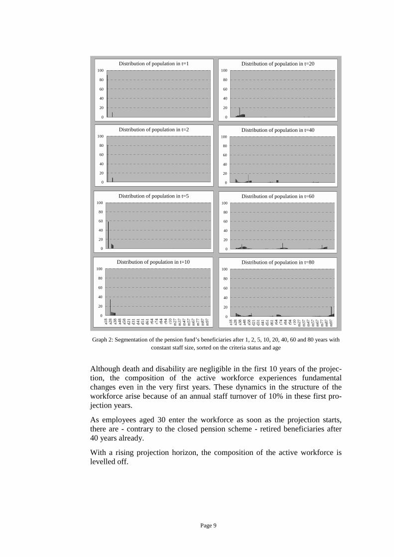
Graph 2: Segmentation of the pension fund’s beneficiaries after 1, 2, 5, 10, 20, 40, 60 and 80 years with

constant staff size, sorted on the criteria status and age

Although death and disability are negligible in the first 10 years of the projec-tion, the composition of the active workforce experiences fundamental changes even in the very first years. These dynamics in the structure of the workforce arise because of an annual staff turnover of 10% in these first pro-jection years.

As employees aged 30 enter the workforce as soon as the projection starts, there are - contrary to the closed pension scheme - retired beneficiaries after 40 years already.

With a rising projection horizon, the composition of the active workforce is levelled off.

3 Salary and savings models

A pension fund’s net cash flow is simply the difference between the contribu-tions collected from the employees and the benefits paid out to the benefit re-cipients. While contributions are calculated with reference to the employer’s salary, benefits are determined with reference to either their salary or their ac-cumulated savings

5 at the time of payment. Accordingly, the derivation of the

fund’s cash flows requires the prior description of the dynamics of these two financial variables.

3.1 Initial distribution of salary and savings

The salary distribution of active employees at inception is exogenously given by the fund. Level and shape of the salary distribution depend on various company-specific criteria such as region, industry, political environment et al.

In order to calculate disability and retirement benefits, the salary vector has also to include salary levels for disabled and retired beneficiaries; these are de-rived from the salaries of active employees at the moment of the status change.

Benefit payments can also be calculated with reference to the accumulated savings, which combine hitherto paid contributions and upon earned interest. These accumulated savings, ordered by status and age, are stored in a vector Bt. The initial vector B0 is exogenous to the fund.

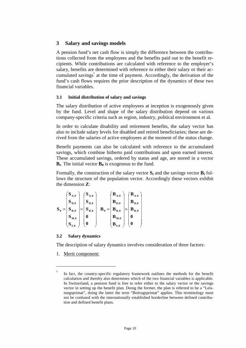
Formally, the construction of the salary vector St and the savings vector Bt fol-lows the structure of the population vector. Accordingly these vectors exhibit the dimension Z:

,

,

,

,

,

,

,

,

,

,

,

,

,

,

,

,

=

=

=

=

0

0

B

B

B

B

B

B

B

B

B

0

0

S

S

S

S

S

S

S

S

S 0R

0D

0A

0S

0M

0R

0D

0A

00R

0D

0A

0S

0M

0R

0D

0A

0

3.2 Salary dynamics

The description of salary dynamics involves consideration of three factors:

1. Merit component:

5 In fact, the country-specific regulatory framework outlines the methods for the benefit

calculation and thereby also determines which of the two financial variables is applicable. In Switzerland, a pension fund is free to refer either to the salary vector or the savings vector in setting up the benefit plan. Doing the former, the plan is referred to be a “Leis-tungsprimat”, doing the latter the term “Beitragsprimat” applies. This terminology must not be confused with the internationally established borderline between defined contribu-tion and defined benefit plans.

The merit component refers to the salary career, which on average is ac-complished over the working years of an active employee. Steepness and curvature of the salary curve are directly linked to the merit policy of the employer.

2. Productivity component:

The second factor that affects equally the salaries of the entire group of employees is labor’s share of productivity gains.

3. Inflation component:

The third factor which is also assumed to have equal impact on all salaries is inflation. The inflation component captures salary increases which aim to maintain purchasing power in an environment of rising prices.

The productivity and the inflation component add up to the scalar g, which in turn drives the level of the salary curve.

For the projections below, it is assumed that the aimed merit scale is already established in the exogenously given salary vector S0. By consequence, the merit component may be neglected and St can be simply derived as:

0t SS ×+= tg)(1

3.3 Dynamics of accumulated savings

The dynamics of the savings vector Bt build on three pillars as well:

1. Exogenous part of savings - Btex:

The exogenously given savings vector at inception generates each year in-terest income at a rate r.

6 Initial savings of retired beneficiaries are pro-

jected at the salary inflation rate g. In other words, retirement benefits get adjusted to inflation.

7 As the projection horizon becomes longer, the im-

pact of the exogenous part of savings on the dynamics of total savings dis-sipates.

2. Endogenous part of savings - Btend:

Accumulated savings get augmented on a periodical basis with annual con-tributions paid by active employees. These are determined as age-specific percentages of the respective salary level. Further on, once paid contribu-tions also earn interest at the rate r. As the projection horizon becomes

6 This rate may be guaranteed or at risk; according to IAS 19 the former refers to a defined

benefit plan , whereas the latter is associated with a defined contribution plan. 7 As for the calculation of total savings of disabled (and early) beneficiaries, it is assumed

that the entire cycle of disabled beneficiaries has become disabled in the previous period. Accordingly, the savings subvector of disabled beneficiaries at time t can be directly de-rived from the savings subvector of active employees at time t-1.

longer, the impact of the endogenous part of savings on the dynamics of total savings becomes stronger and entirely dominates after about 80 pro-jection years.

3. Regulatory part of savings - Btreg:

The here presented regulatory part of savings addresses a peculiarity in de-termining the savings for disabled benefit recipients, which is specific to Swiss pension fund legislation.

Formally, the dynamics of accumulated savings can be represented as:

regt

endt

extt BBBB ++=

The formal derivation of the three pillars of accumulated savings is discussed in the appendix.

Comparing the dynamics of salaries and savings, a methodological difference in the projection of these two vectors has to be highlighted: While an age and status specific salary does not follow the ageing beneficiary through the pro-jection

8, the accumulated savings remain assigned to a specific beneficiary. An

example shall briefly enlighten this different treatment: At inception, some twenty years old person is endowed with an exogenously given salary level and some arbitrary amount of money, which correspond to his accumulated savings. The salary level of this person after ten projection years corresponds to the salary of the person originally aged 30 and meanwhile grown forty 40 years, developed by the salary growth rate g over the projection horizon. On the other hand, the person keeps his original savings throughout the projection. The growth of savings is due to his annual contributions and interest earnings on the particular annual level of the accumulated savings.

There are other methods to extrapolate salary and savings. The projection method chosen in this paper is especially well suited if

1. steepness and shape of the initial salary curve approximately agree with the employer’s ideas on merit scale and

2. pension fund practice with regards to the accumulation of savings or the recent history of salary increases were subject to major changes in the past, so that the endogenously determined and the exogenously given savings level substantially deviate at the start of the projection.

8 Instead, the beneficiary will inherit the salary of his age predecessor, augmented by the

period’s salary inflation rate g.

4 Cash Flow model

Given both the distribution of the fund’s population Pt and the associated sal-ary and saving levels St and Bt at some arbitrary future point in time t, the eco-nomic and formal challenge is to establish a proper link between the popula-tion variables on the one hand and the financial variables on the other hand.

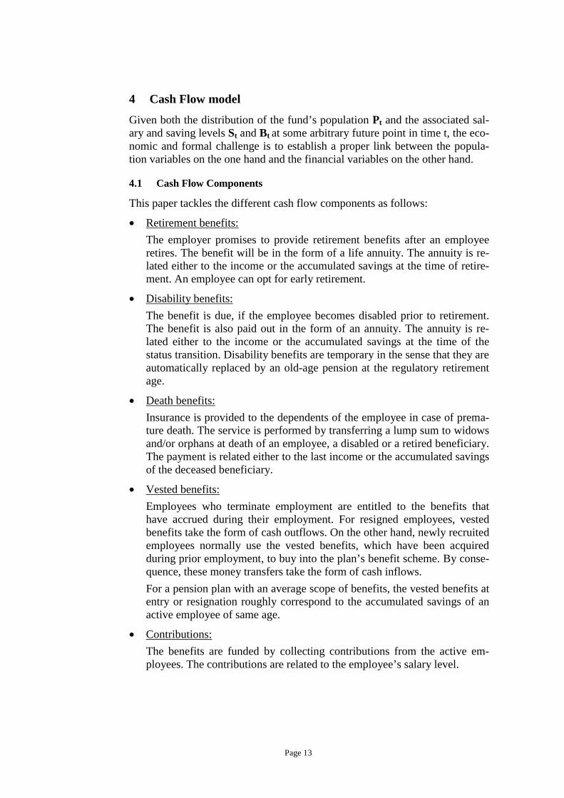
4.1 Cash Flow Components

This paper tackles the different cash flow components as follows:

• Retirement benefits:

The employer promises to provide retirement benefits after an employee retires. The benefit will be in the form of a life annuity. The annuity is re-lated either to the income or the accumulated savings at the time of retire-ment. An employee can opt for early retirement.

• Disability benefits:

The benefit is due, if the employee becomes disabled prior to retirement. The benefit is also paid out in the form of an annuity. The annuity is re-lated either to the income or the accumulated savings at the time of the status transition. Disability benefits are temporary in the sense that they are automatically replaced by an old-age pension at the regulatory retirement age.

• Death benefits:

Insurance is provided to the dependents of the employee in case of prema-ture death. The service is performed by transferring a lump sum to widows and/or orphans at death of an employee, a disabled or a retired beneficiary. The payment is related either to the last income or the accumulated savings of the deceased beneficiary.

• Vested benefits:

Employees who terminate employment are entitled to the benefits that have accrued during their employment. For resigned employees, vested benefits take the form of cash outflows. On the other hand, newly recruited employees normally use the vested benefits, which have been acquired during prior employment, to buy into the plan’s benefit scheme. By conse-quence, these money transfers take the form of cash inflows.

For a pension plan with an average scope of benefits, the vested benefits at entry or resignation roughly correspond to the accumulated savings of an active employee of same age.

• Contributions:

The benefits are funded by collecting contributions from the active em-ployees. The contributions are related to the employee’s salary level.

4.2 Cash Flow Equation

Formally, the link between the population Pt and the financial variable St (Bt) is established by introducing the Z x Z matrix LS (LB). Thus, the equation for the future cash flows is:

)(CF 't 1t

S1t

B1t SLBLP −−− ×+××=

Obviously, understanding the inner structure of the matrices LS and LB marks the final step for the derivation of the pension scheme’s future cash flow pro-file.

In order to establish a direct link between the population distribution Pt and the financial variables St and Bt, the matrices LS and LB must combine two factors:

• Probabilities to migrate from a certain state into another between period t-1 and period t

• Contribution and benefit rates which are paid or received as salary or sav-ing percentages on the occurrence of a specific state transition.

Formally, transition probabilities are captured by the earlier introduced, Z x Z – matrix Π. For the formal representation of the contribution and benefit rates, two time-homogenous Z x Z matrices ΘS and ΘB need to be specified.

9

The element θSij (θB

ij) of the matrix ΘS (ΘB) captures the contribution or bene-fit rate which is applicable when migrating from status i to status j.

Positive (negative) contribution and benefit rates imply a cash inflow (cash outflow) to the fund. The amounts paid or received are calculated by multiply-ing the contribution or benefit rate θS

ij (θBij) with the associated financial vec-

tor entry St-1,i (Bt-1,i).

Multiplying Π and ΘS is an obvious attempt to find a formal representation for LS:

'* SSL ΘΠ ×= and

The same reasoning applies to the matrix LB:

'* BBL ΘΠ ×=

However, it can be shown that the off-diagonale submatrices of LS* and LB* distort the future cash flow representation of the fund. Therefore, LS and LB

9 The parametrization of ΘS and ΘB depends on a plan’s benfit scheme; if for example dis-

ability benefits are calculated in relation to the employee’s level of income, Θ DD S and Θ

AD S have to be parameterized accordingly, whereas the entries in the submatrix Θ DD B and Θ AD

B must be set to 0.

are defined as reduced forms of the matrix products LS* and LB* in the fol-lowing way:

*

*

*

*

*

=

SSS

MMS

RRS

DDS

AAS

S

L0000

0L000

00L00

000L0

0000L

L and

*

*

*

*

*

=

SSB

MMB

RRB

DDB

AAB

B

L0000

0L000

00L00

000L0

0000L

L

The reader should note that the matrices LS and LB are time-invariant.10

Table 1 reveals a lot of the inner structure of the above cash flow equation by discussing each possible migration in turn.

10

This time-invariance stems from the fact that the population dynamics are assumed to fol-low a homogenous Markov process, i.e. that transition probabilities from state i to state j do not change over time.

Possible migrations

Description No. of personsProbability for

migrationContribution / Benefit rate

Reference vector

(dim) (dim) (dim) (dim)

A→AOngoing contributions from active

employeesPA, t-1

(47x1)ΠA→A

(47x47)

cA→A

(47x1)SA, t-1

(47x1)

A→DDisability benefits in the period when

disability occursPA, t-1

(47x1)ΠA→D

(47x47)0

(47x1)-

bA→RS

(47x1)

SA, t-1

(47x1)or

bA→RB

(47x1)

BA, t-1

(47x1)

bA→MS

(47x1)

SA, t-1

(47x1)or

bA→MB

(47x1)

BA, t-1

(47x1)

A→SVested benefits at termination of

employment contract PA, t-1

(47x1)ΠA→M

(47x47)

bA→S

(47x1)BA, t-1

(47x1)

D→AContributions from employees, who get

reactivated from disability PD, t-1

(47x1)ΠD→A

(47x47)

cD→A

(47x1)SD, t-1

(47x1)

bD→DS

(47x1)

SD, t-1

(47x1)or

bD→DB

(47x1)

BD, t-1

(47x1)

bD→RS

(47x1)

SD, t-1

(47x1)or

bD→RB

(47x1)

BD, t-1

(47x1)

bD→MS

(47x1)

SD, t-1

(47x1)or

bD→MB

(47x1)

BD, t-1

(47x1)

bR→RS

(47x1)

SR, t-1

(47x1)or

bR→RB

(47x1)

BR, t-1

(47x1)

bR→MS

(47x1)

SR, t-1

(47x1)or

bR→MB

(47x1)

BR, t-1

(47x1)

S→AVested benefits at entry into

the planf(Pt-1, Π , e, q)

(47x1)1

cS→A

(47x1)BA, t-1

(47x1)

ΠD→M

(47x47)

D→R

D→MLump sum transfers to widows / orphans at

death of disabled emloyeesPD, t-1

(47x1)

Ongoing disability benefits to disabled beneficiaries

PD, t-1

(47x1)ΠD→D

(47x47)

ΠD→R

(47x47)PD, t-1

(47x1)Retirement benefits in the period when

retirement occurs

R→R

ΠA→R

(47x47)

ΠA→M

(47x47)

Retirement benefits in the period when retirement occurs

A→RPA, t-1

(47x1)

A→MLump sum transfers to widows / orphans at

death of active emloyeesPA, t-1

(47x1)

D→D

PR, t-1

(47x1)ΠR→M

(47x47)

ΠR→R

(47x47)Ongoing retiremenet benefits to retired

beneficiaries PR, t-1

(47x1)

CASH FLOW COMPONENTS AT TIME T

R→MLump sum transfers to widows / orphans at

death of retired emloyees

Table 1: Cash Flow components ordered by migration type

The set-up of the table mirrors the structure of the cash flow equation: Column three contains the number of persons in a specific subgroup (Pt-1), the high-lighted columns four and five cover the two factors which constitute the matri-ces LS and LB and column 7 refers to the applicable financial variable (St-1 or Bt-1).

Numeric Example:

The derivation of the fund’s cash flow profile requires assumptions on finan-cial variables such as salary and accumulated savings as well as the specifica-tion of a benefit scheme.

• Salary:

The merit scale of the fund is depicted in Graph 2. An employee aged 18 years earns a salary of CHF 35’000. The salary curve reaches a maximum of CHF 92’000 for employees aged 55 years and remains on that level un-til retirement. Furthermore, the salary curve is assumed to be constant over time. In other words, a salary growth rate g of 0% is assumed.

Merit scale in t=0

0

20'000

40'000

60'000

80'000

100'000

a18

a23

a28

a33

a38

a43

a48

a53

a58

a63

Sal

ary

in C

HF

Graph 3: Average salary career of an active employee

• Contributions:

The fund collects contributions from its active employees. The contribu-tions are calculated as a percentage of current salary. Percentage contribu-tion rates range from 4.00% in the early employment years until 18.00% in the last year prior to retirement.

• Accumulated savings:

In case of resignation, the employee has a claim on his hitherto accumu-lated savings. The savings are calculated as the sum of already collected contributions plus annual interest of 2%.

• Benefits:

The benefit scheme of the fund vests disabled and retired beneficiaries with 60% of their last salary. Resigning beneficiaries receive their accumu-lated savings as a lump sum transfer. The accumulated savings of new em-ployees, which represent a cash inflow to the fund, are assumed to corre-

spond to the level of savings of a current employee of the same age. At the occurrence of a beneficiary’s death, his widow is entitled to a life time an-nuity of 60% of his original claim. The present value of this annuity – dis-counted at a rate of 2% - is paid to the widow as a lump sum transfer at the moment of death.

11

With these assumptions on the benefit scheme and the previously discussed transition rates, the parametrization of the matrices LS and LB is completed.

By applying the cash flow equation to this input information a future cash flow profile as depicted below in Graph 4 is derived.

Future Cash Flows (in CHF) - Closed Pension Scheme

Mortality BenefitsEntry Inflows

Future Cash Flows (in CHF) - Open Pension Scheme

Contributions Retirement Benefits

Exit Benfits Disability Benefits

-6'000'000

-4'000'000

-2'000'000

0

2'000'000

4'000'000

6'000'000

1 6 11 16 21 26 31 36 41 46 51 56 61 66 71 76 81

Projection Periods

-6'000'000

-4'000'000

-2'000'000

0

2'000'000

4'000'000

6'000'000

1 6 11 16 21 26 31 36 41 46 51 56 61 66 71 76 81

Projection Periods

Graph 4: Cash flow projection for the pension fund over the next 85 years sorted on cash flow type and

sex for both a closed and an open system.

11

The fund thereby qualifies as a “Leistungsprimat” under Swiss pension law.

As for the closed pension scheme, the interpretation of the above illustration is straight-forward: the cash inflows in the first 47 projection years correspond to the contributions paid by the beneficiaries during their active career. The growth of these cash inflows is to be attributed to both a rising merit scale and regular increases of the contribution rates. The latter causes the observable jumps in the cash inflows. After 47 years the workforce retires and the fund enters into the decumulation phase. Retirement benefits gradually decrease as the number of beneficiaries diminishes. The cash outflows due to disability also stop after 47 projection years as all disabled beneficiaries are automati-cally transferred to the retirement status at the age of 65.

With regards to the open pension scheme, the shrinking cash flow volume af-ter about 70 projection years may seem a bit puzzling at first sight. However, the entire workforce gets renewed between the projection years 35 and 47 due to retirement of the fund’s first active generation. Thereby, average salaries and contribution rates fall and the generation cycle starts on a lower level again.

5 Conclusion and Outlook

In this paper, a closed form solution for the future cash flows of defined bene-fit pension plans is derived. In a first step, the approach decomposes the cash flow problem into a population model, a salary model and a savings model. In a second step, the partial results are put together to generate the fund’s cash flow profile.

Remarkably, the recursive form of the cash flow equation can be dissolved so that the expected cash flow for some arbitrary future period can be expressed as a function of the exogenously given information on the initial fund popula-tion, the fund’s contribution and benefit scheme, the transition probabilities and the projection variables such as staff growth, salary inflation and interest rate.

The derivation of future cash flows is a premise for a set of financial applica-tions. First, the market value of a financial claim equals its future cash flows, discounted at a risk-adjusted rate. Thus, the cash flow representation of group life insurance contracts mark an important step in the current debate on the fair valuation of pension funds. Second, the plan manager is concerned with the control of the demographic and financial risks involved in providing insurance coverage. The proposed cash flow model equips the plan manager with a pow-erful tool to perform sensitivity analysis and thereby to gain a deeper under-standing of the fund’s actual risk exposure.

However, the application of the cash flow equation in the fields of finance ap-pointed above requires still some further research.

Appendix

Projection of the exogenous part of savings Btex

The projection of the exogenous part of savings Btex requires the specification

of a Z x Z matrix T:

=

=

00000

00000

00T00

00000

00TTT

TTTTT

TTTTT

TTTTT

TTTTT

TTTTT

T RR

ARADAA

SSSMSRSDSA

MSMMMRMDMA

RSRMRRRDRA

DSDMDRDDDA

ASAMARADAA

with

+

++

=

+

++

==

0..000

g1..000

..........

0..g100

0..0g10

0..000

r1..000

..........

0..r100

0..0r10

RRADAA TTT

Finally, the only non-zero value of TAR equals (1+r) and is located in the last row and the first column of the submatrix.

On the one hand, the matrix TAA ensures that the exogenously given savings earn annual interest. On the other hand, accumulated savings for retired bene-ficiaries grow at the rate g instead of r, mirroring the fact that the reference value for calculating retirement benefits has to be adjusted to inflation. Interest on the other hand must not be added to the savings of retired beneficiaries, as interest is implicitly assumed while converting the accumulated savings into an annuity at retirement. The conversion factor is dependant on mortality and morbidity assumptions as well as the presumed interest rate.

With the above specification of T the dynamics of the exogenous part of sav-ings Bt

exbecome:

tex0

ext TBB ×= '

Projection of the endogenous part of savings Btend

The endogenous part of savings Btend contains all contributions paid in the

course of the projection and earned upon interest. The derivation of Btend re-

quires some formal groundwork:

First, an indicator function I(x) is defined as follows:

<≥

=0 xif ; 0

0 xif ; 1 I(x)

Second a 47 x 47, strictly upper triangular matrix QtA is introduced

12. The ma-

trix element (i, i+j) of QtA is defined as:

(1,46) j (1,47), i j)-I(tg1

r1 j)i(i,Q

1-j

At ∈∈∀×

++=+

Third a 47 x 40 13 matrix Qt

R is introduced. The matrix element (i, j) of QtR is

defined as:

(1,40) j (1,47), i 47)-ij-I(tg1

r1 j)(i,Q

i-47

Rt ∈∈∀+×

++=

Fourth, QtA and Qt

R are used for constructing a 47 x Z matrix as follows:

( ) )( 0QQpartQQQ Rt

At

At

Att = ,

where the 47 x 7 matrix part(QtA) corresponds to the last seven columns of

the matrix QtA and 0 is a null matrix of order 47 x (Z – 141).

14

Fifth, a 47 x 47 matrix C is specified. The diagonal elements of C correspond to the age-specific regulatory contribution rates for active employees.

With Qt and C at hand, the dynamics for Btend become:

t0Aend

t QCSB ×××+= ',

1-t' g)(1

Intuitively, Qt adjusts the product of the regulatory contribution rates (C) and the current salary level ((1+g)t-1 x SA,0) by taking into account the following considerations:

• Previous contributions earn interest

• Previous contributions have been determined with regards to a lower salary level

• Contributions can only be considered for the length of the projection pe-riod

12

As the maximum (minimum) age of active employees is 64 years (18 years), there are ex-actly 47 separate age buckets for active employees in the system.

13 As the maximum (minimum) age of active employees is 104 years (65 years), there are

exactly 40 separate age buckets for active employees in the system. 14

The sole object of the null submatrix is to avoid dimension mismatch when multiplying matrices in the projection.

Projection of the regulatory part of savings Btreg

As stated earlier, the regulatory part of savings Btreg addresses a peculiarity of

the Swiss pension fund legislation: In a Swiss defined contribution plan15, dis-

ability benefits are calculated with reference to accumulated savings. It is straightforward that these benefits will be very low for young employees due to a low reference value. Accordingly, accumulated savings of a newly dis-abled beneficiary are augmented by an amount, which approximately equals his current contribution level multiplied by the current salary times the missing years to retirement.

Formally, Btreg can be derived as:

RCtrB regt ××+= '1-t' )(g)(1

The 47 x Z - matrix R, which covers the necessary salary information, is specified as:

( )rDl 0R0R = ,

where the null matrix 0l (0r) left (right) to RD has the size 47 x 47 (47 x [Z-94]) and the 47 x 47 submatrix RD is illustrated below:

S..SS0

..........

0..SS0

0..0S0

0..000

A63,0A19,0A18,0

A19,0A18,0

A18,0

=DR

15

In Swiss pension fund practice the border established between a defined contribution and a defined benefit plan is somewhat different to the international standard: whereas the in-ternational definition of a defined benefit plan refers to a plan which incorporates any sort of a benefit guarantee, benefit guarantees are present in both defined contribution and de-fined benefit plans in Switzerland. A Swiss defined benefit plan guarantees specified rates of the last salary in case of disability, death or retirement, whereas in a Swiss defined con-tribution plan these benefits are calculated with reference to the accumulated savings. However, savings must be credited minimum interest each year. The minimum interest rate is determined by the regulator.

References

Bertschi, L., Ebeling, S., Reichlin, A., 2003, „Dynamic Asset Liability Man-agement: A Profit Testing Model for Swiss Pension Funds“, 34th ASTIN In-ternational Colloquium

Chang, S., and Cheng, H., 2002, “Pension Valuation under Uncertainties: Im-plementation of a Stochastic and Dynamic Monitoring System”, Journal of Risk & Insurance, Vol. 69, No. 2, 171-192

Janssen, J., 1966, “Application des processus semi-markoviens à un problème d’invalidité“, Bulletin de l’ Association Royale des Actuaries Belges, 63, 35-52

Janssen, J., and Manca, R., 1997, “A Realistic Non-Homogenous Stochastic Pension Fund Model on Scenario Basis”, Scandinavian Actuarial Journal, 2: 113 - 137

Koller, M., 2000, “Stochastische Modelle in der Lebensversicherung”, Springer Verlag

Papadopoulou, A. A., 2001, “Rewards in non homogenous semi Markov sys-tems in discrete time”, Proceedings of the 10th International Symposium on ASMDA 2001, G. Govaert, J. Janssen, N. Limnios Eds, 819 - 824

Papadopoulou, A. A., and Vassiliou, P. C., 1999, “Continuous time non ho-mogenous semi-Markov systems”, in Janssen, J., and Limnios, N., “Semi-markov Models and Applications”, Chapter 15, 241 – 251, Kluwer Academic Publishers, Dordrecht

Ruhdorfer, M., 1988, „Simulationen in der betrieblichen Altersversorgung: Ein Markov-Modell und Abschätzungen für die Anzahl der Simulationen“, Dissertation, Universität der Bundeswehr München, Fakultät für Elektrotechnik

Winklevoss, H., 1993, “Pension Mathematics With Numerical Illustrations”, 2nd ed., University of Pennsylvania Press

Wolthuis, H., 1994, „Life Insurance Mathematics (The Markovian Model)“, Education Series Volume 2, CAIRE, Brussels

PROJECTING PENSION FUND CASH FLOWS - HOME (EN) · PDF filePage 1 PROJECTING PENSION FUND CASH...

Documents

Transcript of PROJECTING PENSION FUND CASH FLOWS - HOME (EN) · PDF filePage 1 PROJECTING PENSION FUND CASH...