Projecting impacts of climate change on surface watertemperatures of a large subalpine lake: Lake Tahoe, USA

Ka Lai Christine Ngai & Brian J. Shuter &

Donald A. Jackson & Sudeep Chandra

Received: 19 August 2009 /Accepted: 7 January 2013 /Published online: 12 February 2013# Springer Science+Business Media Dordrecht 2013

Abstract Predicted increases in atmospheric CO2 concentration are expected to causeincreases in air temperatures in many regions around the world, and this will likely lead toincreases in the surface water temperatures of aquatic ecosystems in these regions. Usingdaily air and littoral water temperature data collected from Lake Tahoe, a large sub-alpinelake located in the Sierra Nevada mountains (USA), we developed and tested an empiricalapproach for constructing models designed to estimate site-specific daily surface watertemperatures from daily air temperature projections generated from a regional climatemodel. We used cluster analysis to identify thermally distinct groups among sampled siteswithin the lake and then developed and independently validated a set of linked regressionmodels designed to estimate daily water temperatures for each spatially distinct thermalgroup using daily air temperature data. When daily air temperatures projections, generatedfor 2080–2099 by a regional climate model, were used as input to these group models,projected increases in summer surface water temperatures of as much as 3 °C were projected.This study demonstrates an empirical approach for generating models capable of using dailyair temperature projections from established climate models to project site specific impactson littoral surface waters within large limnetic ecosystems.

Climatic Change (2013) 118:841–855DOI 10.1007/s10584-013-0695-6

K. L. C. Ngai (*) : B. J. Shuter :D. A. JacksonDepartment of Ecology and Evolutionary Biology, University of Toronto, 25 Harbord St, Toronto, ONM5S 3G5, Canadae-mail: cngai@cabnr.unr.edu

B. J. ShuterHarkness Laboratory of Fisheries Research, Aquatic Ecosystem Science Section, Ontario Ministry ofNatural Resources, 300 Water St, Peterborough, ON K9J 8M5, Canada

S. ChandraDepartment of Natural Resources and Environmental Science, Aquatic Ecosystems Analysis Laboratory,University of Nevada- Reno, 1664 N. Virginia St., MS 0186, Reno, NV 89557, USA

Present Address:K. L. C. NgaiDepartment of Natural Resources and Environmental Science, Aquatic Ecosystems Analysis Laboratory,University of Nevada- Reno, 1664 N. Virginia St, MS 0186, Reno, NV 89557, USA

AbbreviationsSWT Surface water temperatureOEI Offshore and exposed inshoreEI Enclosed inshore

1 Introduction and background

Surface water temperatures of freshwater ecosystems will respond strongly to anticipatedincreases in global atmospheric temperatures (Robertson and Ragotzkie 1990; Hondzo andStefan 1993). Warmer water temperatures can lead to significant changes in the physical (e.g.water clarity, and ice cover), chemical (e.g. pH and nutrient availability, dissolved oxygen level)and biological (e.g. growth and persistence of organisms, invasive species establishment)processes and attributes of freshwater lake systems (Shuter and Meisner 1992; Schindler2001; Rahel and Olden 2008). Projecting how water temperatures of lake systems will respondto climate change can be useful for anticipating andmitigating the ecological impacts of climatechange on these systems. However, to date climate change projections for freshwater systemshave focused on among-lake differences across large regional landscapes (e.g. Sharma et al.2007; Trumpickas et al. 2009)—methods incorporating downscaled models operating atsmaller spatial scales, or within large lake systems, are rare.

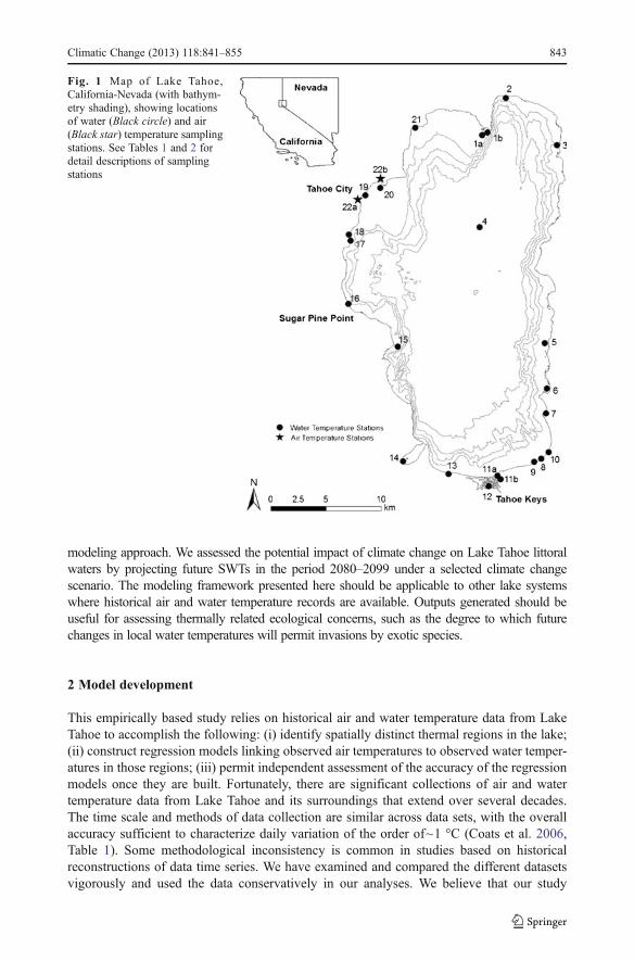
In this study, Lake Tahoe (39°6′N, 120°6′W), a large (avg. depth: 305 m, surface area:500 km2) oligotrophic, subalpine (1,898 m above sea level) lake (Fig. 1), situated on theborders of California and Nevada, is used as a case study to explore an empirical method forprojecting within lake, site-specific nearshore future surface water temperatures(SWTs - Moyle 2002). Lake Tahoe is a suitable case study system for several reasons.Firstly, locations inland or at higher elevations may be climatically more vulnerable andshould have greater temperature and precipitation responses to climate change than coastallocations, or areas at lower elevations (Snyder et al. 2002). Secondly, studies exploringpossible future climates in California have generally projected air temperature increasesranging from 1 to 6 °C by 2,100, depending on the greenhouse gas emission scenario usedand time period set by the climate model (Kim 2001; Hayhoe et al. 2004; Duffy et al. 2006).For example, down-scaled output of the Geophysical Fluid Dynamics Laboratory globalclimate model (GFDL CM2.1: A2 scenario) shows a 4–5 °C increase in Tahoe basin’s airtemperature over the 21st century (Coats et al. 2013). Thirdly, a general warming trend hasalready been documented for Lake Tahoe: over the period 1992–2008, mean summer watertemperatures have been increasing at a rate of 0.11 °C per year (Schneider et al. 2009).Finally, Lake Tahoe is an important national resource, especially for the two western states itborders; the lake is an important source of freshwater for residents in the surrounding areaand the extraordinary clarity of its water has made it one of three water bodies in the westernUnited States to be designated an Outstanding National Resource Water under the CleanWater Act (TRPA 2009). Thus, assessing potential impacts of climate change on the littoralwaters of Lake Tahoe is of national interest, as well as of interest to many local stakeholders.

The primary objective of this paper is to present a method for constructing empirical modelsdesigned to estimate downscaled, site-specific future water temperatures from future air temper-atures generated by a regional climate model. Instead of generating lake-wide averages, thismodeling approach takes into account the temporally consistent, spatial heterogeneities in SWTthat are often found in large lakes (e.g. Finlay et al. 2001). Using several historical air and SWTdatasets available for Lake Tahoe, we tested the effectiveness and practicality of the proposed

842 Climatic Change (2013) 118:841–855

modeling approach. We assessed the potential impact of climate change on Lake Tahoe littoralwaters by projecting future SWTs in the period 2080–2099 under a selected climate changescenario. The modeling framework presented here should be applicable to other lake systemswhere historical air and water temperature records are available. Outputs generated should beuseful for assessing thermally related ecological concerns, such as the degree to which futurechanges in local water temperatures will permit invasions by exotic species.

2 Model development

This empirically based study relies on historical air and water temperature data from LakeTahoe to accomplish the following: (i) identify spatially distinct thermal regions in the lake;(ii) construct regression models linking observed air temperatures to observed water temper-atures in those regions; (iii) permit independent assessment of the accuracy of the regressionmodels once they are built. Fortunately, there are significant collections of air and watertemperature data from Lake Tahoe and its surroundings that extend over several decades.The time scale and methods of data collection are similar across data sets, with the overallaccuracy sufficient to characterize daily variation of the order of~1 °C (Coats et al. 2006,Table 1). Some methodological inconsistency is common in studies based on historicalreconstructions of data time series. We have examined and compared the different datasetsvigorously and used the data conservatively in our analyses. We believe that our study

Fig. 1 Map of Lake Tahoe,California-Nevada (with bathym-etry shading), showing locationsof water (Black circle) and air(Black star) temperature samplingstations. See Tables 1 and 2 fordetail descriptions of samplingstations

Climatic Change (2013) 118:841–855 843

provides a sound demonstration of how to compensate for such inconsistencies and generateuseful results.

2.1 Temperature data sources

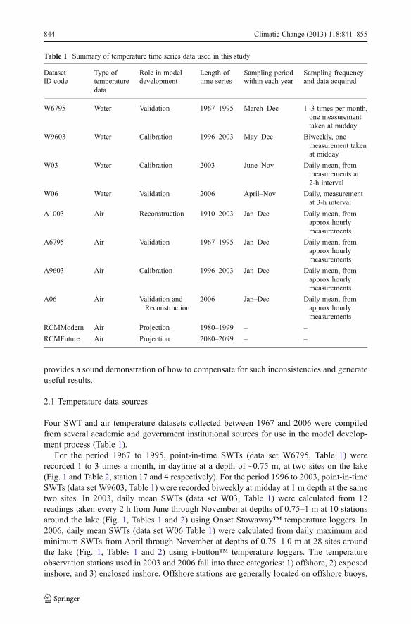
Four SWT and air temperature datasets collected between 1967 and 2006 were compiledfrom several academic and government institutional sources for use in the model develop-ment process (Table 1).

For the period 1967 to 1995, point-in-time SWTs (data set W6795, Table 1) wererecorded 1 to 3 times a month, in daytime at a depth of ~0.75 m, at two sites on the lake(Fig. 1 and Table 2, station 17 and 4 respectively). For the period 1996 to 2003, point-in-timeSWTs (data set W9603, Table 1) were recorded biweekly at midday at 1 m depth at the sametwo sites. In 2003, daily mean SWTs (data set W03, Table 1) were calculated from 12readings taken every 2 h from June through November at depths of 0.75–1 m at 10 stationsaround the lake (Fig. 1, Tables 1 and 2) using Onset Stowaway™ temperature loggers. In2006, daily mean SWTs (data set W06 Table 1) were calculated from daily maximum andminimum SWTs from April through November at depths of 0.75–1.0 m at 28 sites aroundthe lake (Fig. 1, Tables 1 and 2) using i-button™ temperature loggers. The temperatureobservation stations used in 2003 and 2006 fall into three categories: 1) offshore, 2) exposedinshore, and 3) enclosed inshore. Offshore stations are generally located on offshore buoys,

Table 1 Summary of temperature time series data used in this study

DatasetID code

Type oftemperaturedata

Role in modeldevelopment

Length oftime series

Sampling periodwithin each year

Sampling frequencyand data acquired

W6795 Water Validation 1967–1995 March–Dec 1–3 times per month,one measurementtaken at midday

W9603 Water Calibration 1996–2003 May–Dec Biweekly, onemeasurement takenat midday

W03 Water Calibration 2003 June–Nov Daily mean, frommeasurements at2-h interval

W06 Water Validation 2006 April–Nov Daily, measurementat 3-h interval

A1003 Air Reconstruction 1910–2003 Jan–Dec Daily mean, fromapprox hourlymeasurements

A6795 Air Validation 1967–1995 Jan–Dec Daily mean, fromapprox hourlymeasurements

A9603 Air Calibration 1996–2003 Jan–Dec Daily mean, fromapprox hourlymeasurements

A06 Air Validation andReconstruction

2006 Jan–Dec Daily mean, fromapprox hourlymeasurements

RCMModern Air Projection 1980–1999 – –

RCMFuture Air Projection 2080–2099 – –

844 Climatic Change (2013) 118:841–855

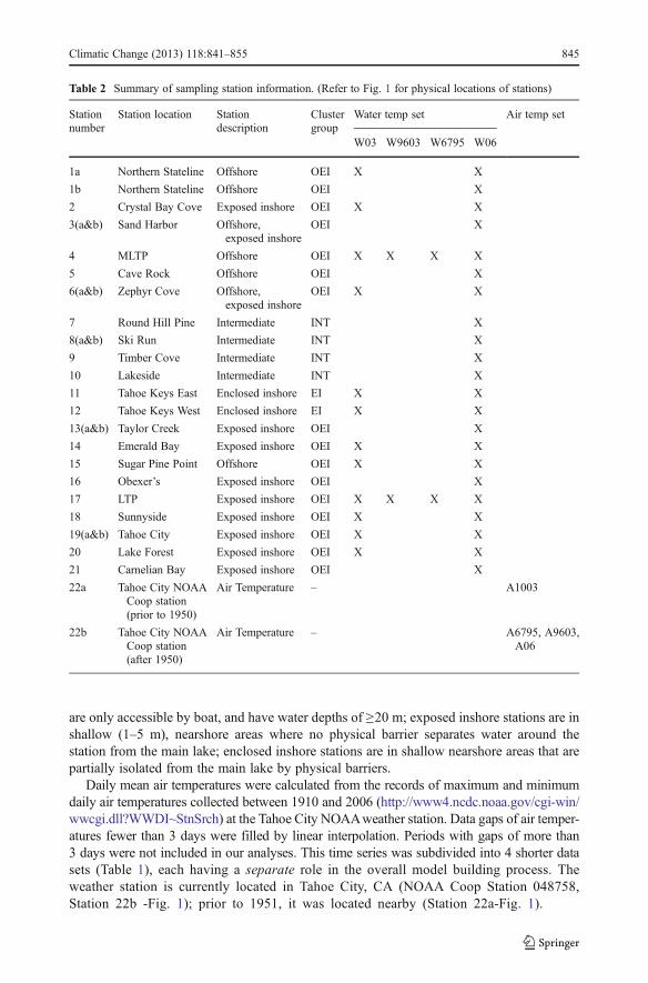
are only accessible by boat, and have water depths of ≥20 m; exposed inshore stations are inshallow (1–5 m), nearshore areas where no physical barrier separates water around thestation from the main lake; enclosed inshore stations are in shallow nearshore areas that arepartially isolated from the main lake by physical barriers.

Daily mean air temperatures were calculated from the records of maximum and minimumdaily air temperatures collected between 1910 and 2006 (http://www4.ncdc.noaa.gov/cgi-win/wwcgi.dll?WWDI~StnSrch) at the Tahoe City NOAAweather station. Data gaps of air temper-atures fewer than 3 days were filled by linear interpolation. Periods with gaps of more than3 days were not included in our analyses. This time series was subdivided into 4 shorter datasets (Table 1), each having a separate role in the overall model building process. Theweather station is currently located in Tahoe City, CA (NOAA Coop Station 048758,Station 22b -Fig. 1); prior to 1951, it was located nearby (Station 22a-Fig. 1).

Table 2 Summary of sampling station information. (Refer to Fig. 1 for physical locations of stations)

Stationnumber

Station location Stationdescription

Clustergroup

Water temp set Air temp set

W03 W9603 W6795 W06

1a Northern Stateline Offshore OEI X X

1b Northern Stateline Offshore OEI X

2 Crystal Bay Cove Exposed inshore OEI X X

3(a&b) Sand Harbor Offshore,exposed inshore

OEI X

4 MLTP Offshore OEI X X X X

5 Cave Rock Offshore OEI X

6(a&b) Zephyr Cove Offshore,exposed inshore

OEI X X

7 Round Hill Pine Intermediate INT X

8(a&b) Ski Run Intermediate INT X

9 Timber Cove Intermediate INT X

10 Lakeside Intermediate INT X

11 Tahoe Keys East Enclosed inshore EI X X

12 Tahoe Keys West Enclosed inshore EI X X

13(a&b) Taylor Creek Exposed inshore OEI X

14 Emerald Bay Exposed inshore OEI X X

15 Sugar Pine Point Offshore OEI X X

16 Obexer’s Exposed inshore OEI X

17 LTP Exposed inshore OEI X X X X

18 Sunnyside Exposed inshore OEI X X

19(a&b) Tahoe City Exposed inshore OEI X X

20 Lake Forest Exposed inshore OEI X X

21 Carnelian Bay Exposed inshore OEI X

22a Tahoe City NOAACoop station(prior to 1950)

Air Temperature – A1003

22b Tahoe City NOAACoop station(after 1950)

Air Temperature – A6795, A9603,A06

Climatic Change (2013) 118:841–855 845

2.2 Identifying spatial heterogeneity in water temperatures

Spatial heterogeneity in SWTs is typical in large lakes (e.g. Finlay et al. 2001) and needs tobe quantified when developing within lake-scale empirical SWT projection models. We usedvariation analysis and cluster analysis of the concurrent, site-specific daily water temperaturetime series from both 2003 and 2006 to identify temporally consistent spatial heterogeneityin SWTs across Lake Tahoe.

We used variation analysis to quantify seasonal changes in the range and standarddeviation of daily mean SWTs recorded across all sampled sites. We used clusteranalysis to determine if this variation was the product of temporally consistent spatialheterogeneity among sites. To facilitate partitioning and to minimize the effect ofmissing data, we focused our cluster analyses on the season identified by variationanalysis as the season where among-site SWT variation was greatest. We used theagglomerative hierarchical method and Euclidean distances, as embodied in theAGNES programming function in S-PLUS™ (see S-PLUS help manual for detaileddescription of the program—Kaufman and Rousseeuw 1990). Results from bothcomplete linkage (furthest neighbour) clustering and UPGMA (Unweighted PairGroup Method with Arithmetic means) clustering were considered (Legendre andLegendre 1998; Gordon 1999). Consensus tree analysis (Gordon 1987) and theCI(C) index (Rohlf 1982; NT-SYS numerical-taxonomy package; Rohlf et al. 1982)were used to assess dendrogram similarity. The Majority-Rule Consensus tree (Gordon1987) and the CI(C) index (Rohlf 1982; Jackson et al. 1989) both measure agreementbetween dendograms. CI(C) values can range between 0 and 1 (Rohlf 1982; Jacksonet al. 1989).

In both 2003 and 2006, spring and early summer was the period of greatest spatialvariation in SWTs—a finding similar to that reported by Finlay et al. (2001). We usedcluster analysis on data from the period in each year when both the range and standarddeviation of across-site temperatures were near their maximum values (Julian day 158–195 for 2003 and 166–213 for 2006) and we observed a consistent clustering of sites inboth years. There were 3 thermally distinct clusters (Fig. 2): (i) enclosed inshore (EI)sites - located within the Tahoe Keys (the largest marina complex located in the southside of the lake- Fig. 1 and Table 2, station 11a,b and 12); these sites were consistentlywarmer in late spring-early summer and cooler in the fall than the other sites; (ii)offshore and exposed inshore (OEI) sites - located offshore, or inshore on exposedshorelines; these sites were consistently cooler than other sites in spring and summer,and warmer in fall; 3) intermediate (INT) sites - located mostly along the southernshore; these sites exhibited intermediate temperatures in all seasons. We used twoclustering methods on the same sets of data, (i.e. UPGMA and complete linkageclustering) to verify that the groupings identified were robust to the choice of clusteringmethod. For W03 and W06, both the consensus tree analysis and the consensus index(CI(C) =1.0 and 0.84 respectively) indicated that the dendrograms from the twomethods were similar and consistent.

2.3 Modeling spatial heterogeneity in water temperatures

We focused our modeling work on constructing SWT projection models for the OEI (coolestspring and summer, warmest fall) and EI (warmest spring and summer, coolest fall) clustersof sites, with the intent of capturing the full range of horizontal thermal variability likely tobe observed under climate change.

846 Climatic Change (2013) 118:841–855

2.3.1 OEI base model development and validation

Models for predicting SWTs from air temperatures are common in the literature (e.g. Shuteret al. 1983; Livingstone and Lotter 1998; Kettle et al. 2004) and several (Matuszek andShuter 1996; Groeger and Bass 2005; Livingstone and Padisak 2007) demonstrate that dailySWTs can be accurately predicted using various combinations of lagged running averages ofdaily air temperatures. We followed Matuszek and Shuter (1996) because their model issimple and was validated with data from several (14) lakes covering a wide range of areas,depths and shapes. Matuszek and Shuter (1996) also demonstrated that air temperatures usedfor their model input need not be collected at a point close to the lake, as long as it is withinthe same regional climatic zone as the lake (e.g. within~300 km for the lakes theyexamined). The SWT model for a particular thermal cluster of sites has the following

a.

b.

Fig. 2 a Dendrograms (Cluster Analysis) of 2006 late spring/early summer (Julian day:166–213) dailysurface-water temperatures (SWT) at various sites across Lake Tahoe based on Unweighted Pair GroupMethod with Arithmetic means (UPGMA). The dissimilarity between sites in terms of daily SWT can bedetermined from the height at which various sites are joined into groups. See Fig. 1 for site locations. b 2006daily SWT from early spring to late fall collected by 27 temperature probes at 21 sampled sites. Bluerepresents temperature regimes of offshore and exposed inshore (OEI) sites, red represents temperatureregimes of highly enclosed inshore (EI) sites (i.e. Tahoe Keys at the south side of the lake), and greenrepresents other south shore sites INT)

Climatic Change (2013) 118:841–855 847

structure:

SWTyday ¼ C0 þ C1 ATemp5ð Þ þ C2 ATemp20ð Þ þ C3 ydayð Þ þ C4 ydayð Þ2 ð1Þ

where SWTyday is the daily mean SWT (°C) on Julian day yday, C0−4 are cluster-specific constants, ATemp5 is the 5-day running mean of daily average air temper-atures (°C) for the 5 day period ending with yday, and ATemp20 is the 20-dayrunning mean of daily average air temperature (°C) for the 20 day period endingwith yday. In the original formulation of the model, Matuszek and Shuter (1996)included an additional term to allow for the effects of ice cover. However, Rennie(2003) reported that this term was not significant in his application of the model, andLake Tahoe does not freeze over (Jassby et al. 2001; Coats et al. 2006), thus this termwas not included in our model.

The Matuszek and Shuter (1996) model was designed to capture the empirical linkagebetween SWTs and air temperatures, when daily SWTs fluctuate in response to the annualrise and fall of air temperatures in the “non-winter period” of a year. Therefore, the model isnot appropriate for projecting SWTs during winter, when Tahoe water temperatures stabilizeand become relatively independent of air temperature. In our case study, we defined the non-winter period as the period when daily SWTs are consistently above the winterthreshold temperature of 4.6 °C. This threshold temperature was selected based onlong term lake monitoring records which show that, during winter, Lake Tahoe SWTsremain at~4.6 °C despite changes in winter air temperatures (Strub and Powell 1987;Jassby et al. 2001).

We used linear regression to fit OEI SWT data (data sets W9603 and W03, pruned toinclude only values from the non-winter period and averaged across OEI sites within a day)to Tahoe City air temperature data (dataset A1003) and generated the following OEI basemodel (R2=0.93; RMSE=0.88; N=312; RMSE values for individual years range from 0.66to 1.35):

SWTyday ¼ �20:6783þ 0:16255 ATemp5ð Þ þ 0:29978 ATemp20ð Þ þ 0:26121 ydayð Þ� 5:35E�4 ydayð Þ2 ð2Þ

We validated this model using two independent SWT datasets (W6795 and W06),one from an historical period (1967–95) prior to that used to derive the model (1996–2003) and the other from a period (2006) subsequent to that used to derive the model.Validation results for both time periods demonstrated that, overall, the OEI modelprovided unbiased predictions of daily temperatures (Fig. 3a), with relatively smalland consistent within- and between-year error levels: (i) for the 1967–1995 period,overall mean residual=0.0482 °C; range for yearly mean residuals (N=29): −0.94 to0.89 °C; range for yearly RMSE values: 0.73 to 1.87; 85 % of all daily forecasts(N=569) were within +/−1.5 °C of observed values (ii) for 2006, RMSE=0.89; 90 %of all daily projections (N=148) were within +/− 1.5 °C of observed values. However,the monthly residual plot (Fig. 3b) does reveal that the accuracy of model predictionsis reduced for those periods (March, April and November) when SWTs are just risingfrom, or closely approaching the winter threshold temperature. For these months,some residual values were derived from predicted values that were set to 4.6 °Cbecause the raw values from Eq. (2) were<4.6C.

848 Climatic Change (2013) 118:841–855

2.3.2 EI model development and validation

Since only 2 years (2003, 2006) of data were available from EI sites, we could not follow thesame modeling approach as we used for OEI sites. However, for those years whereconcurrent OEI and EI data were available, mean daily EI SWTs were linked to mean dailyOEI SWTs by strong, but distinctly different, linear relationships during the spring warmingperiod (R2=0.59) and the fall cooling period (R2=0.98). Within each season, there wererelatively small (but statistically significant ANCOVA spring p=0.03 and fall p<0.001)interannual differences in the parameter estimates for these regression lines: (i) For Spring,2003 and 2006 slope values were 0.6984 and 0.9318 respectively, the pooled slope was0.8946 and, overall, the 2003 relationship was elevated above the 2006 relationship suchthat, for any given OEI value, the 2003 EI value was~1 °C higher than the 2006 EI value;

a

b

1967

1968

1969

1970

1971

1972

1973

1974

1975

1976

1977

1978

1979

1980

1981

1982

1983

1984

1985

1986

1987

1988

1989

1990

1991

1992

1993

1994

1995

-6-5-4-3-2-10123456

Res

idua

l (°C

)

Year

3 4 5 6 7 8 9 10 11 12

-6-5-4-3-2-10123456

Res

idua

l (°C

)

Month

Fig. 3 Historical reconstruction testing (1967–1995): Residual temperatures (observed-predicted) summa-rized for (a) annual and (b) monthly time frames. Predictions were generated using OEI base model and dailyair temperatures recorded in 1967–1995, and were compared to observed offshore and exposed inshore (OEI)water temperatures collected in 1967–1995. The lines in the boxes represent the 25 %, 50 % and 75 %quartiles. Extreme values are displayed as “Asterisk” for possible outliers (exceeds box boundaries by morethan 1 1/2 times the height of the box) and “O” for probable outliers (exceeds box boundaries by more than 3times the height of the box)

Climatic Change (2013) 118:841–855 849

(ii) For Fall, 2003 and 2006 slope values were 1.6002 and 1.7782, respectively, the pooledvalue was 1.7252 and, overall, for any given OEI value, the 2003 EI value was similar to the2006 EI values. Given these results, we chose to model EI SWTs using values from the OEIbase model as input to two separate linear relationships, one linking spring EI values tospring OEI values and the other linking fall EI values to fall OEI values, with the day of theyear with the highest OEI SWT value (HTD) used to separate the spring warming and fallcooling phases of the year. Regression analysis of the pooled 2003 and 2006 data was usedto derive the final model (R2=0.8 and 0.85, Mean residual=0.3 °C and 0.22 °C, RMSE=1.39and 1.33, for 2003 and 2006 respectively):

SWT ydayð ÞEI warmingð Þ ¼ 0:8946 SWT ydayð ÞOEI all yday�HTDð Þ þ 5:6391SWT ydayð ÞEI coolingð Þ ¼ 1:7252 SWT ydayð ÞOEI all yday�HTDð Þ � 12:5718

ð3Þ

where: SWT(yday)EI is the predicted daily EI SWT value for Julian day yday ; SWT(yday)OEI isthe OEI SWT value generated from the OEI base model for yday and HTD is the Julian daywhere SWT(yday)OEI reaches its maximum value.

An independent EI SWT dataset from 2001 was used to validate the EI model. The R2

value between observed and predicted values was high (0.84) while both mean residual andRMSE value (0.875 °C and 2.13) were only moderately higher than the RMSE and residualvalues for 2003 and 2006.

3 Model applications

3.1 Reconstruction of current SWTs and projection of future SWTs

We used observed daily air temperature data (1910–2006) collected from Tahoe Cityweather station to reconstruct historical daily SWTs using the calibrated and validatedempirical models. Projected (2080–2099) daily air temperatures generated by the regionalclimate model (RCM) published in Snyder and Sloan (2005) were used to derive future SWTprojections for Lake Tahoe under one climate change scenario. The projected air temperaturedata were provided by Dr. Mark A. Snyder from the Department of Earth and PlanetarySciences, University of California, Santa Cruz.

3.1.1 Future climate change scenario

In Snyder and Sloan (2005), possible changes in California climate for the period from 1980–99(the ‘Modern’ period) to 2080–99 (the ‘Future’ period) were examined using the RCM -RegCM2.5. The output from an atmosphere—ocean general circulation model (AOGCM)—National Center for Atmospheric Research (NCAR) Climate System Model version 1.2 (seeSnyder and Sloan 2005 for model details) was used to drive the RCM. For the AOGCM runs,CO2 concentrations were updated each year based on 1) observed values of greenhouse gases(338–369) for the “Modern” case, and 2) projected values from the IPCC A1 scenario for the“Future” case. The CO2 values used in the RCM for “Modern (1980–99)” and “Future (2080–99)” cases were fixed at 353 and 660 ppm respectively, as the RCM cannot handle time-varyinggreenhouse gases (Snyder and Sloan 2005). Snyder and Sloan (2005) demonstrated that theRCM reproduced reasonably accurate monthly average temperature values for the Modernperiod, with an average underestimation of approximately 2 to 4 °C. It was also able to capturethe seasonal cycle of temperatures for all months examined.

850 Climatic Change (2013) 118:841–855

This RCMprovides output at a much higher resolution (40 km×40 km) than a typical globalclimate model (GCM) (~280 km×280 km), and is better at capturing regional variation inclimate, especially for areas like California which are topographically complex (Bell et al. 2004;Snyder and Sloan 2005). Four grid cells from the RCM cover the entire range of Lake Tahoe.We compared past air temperatures (1980–1999) collected from the Tahoe City weather stationwith simulated air temperatures generated by the RCM for the same time period to identify thegrid cell output that was most comparable to observed Tahoe City values.

Before future air temperature projections generated from the RCM could be used as inputfor our SWT projection models, pre-treatment of the raw RCM output was required toaddress the following limitations of RCM model: (i) daily variation in simulated RCM airtemperature values tends to exceed observed variation due to numerical properties of thesimulation algorithms (M. A. Snyder, University of California- Santa Cruz, personal com-munication); (ii) systematic bias in simulated values can be present due to inherent discrep-ancies in the GCM output that drives the RCM (Snyder et al. 2002); (iii) each gridtemperature value from the RCM represents the average temperature within a 40×40kmgrid cell, thus variation at smaller spatial scales cannot be captured accurately by the RCMmodel. We dealt with these limitations by (i) using a 5 day running average (running mean ofa 5 day period ending with the current day) of the simulated RCM daily air temperatures asinput to our empirical models to reduce the simulated daily variations to values comparable(< 30 %) to observed daily variations; (ii) applying to these daily running averages, acorrection factor based on the monthly median differences between observed and simulatedair temperatures for the 1980–99 “modern” period.

3.1.2 Future SWT projections for Lake Tahoe

Daily SWT projections generated by the OEI base model and the supplementary EI model weresummarized as annual averages (Fig. 4).Winter values were generated by enforcing a minimum

Fig. 4 Past, present, and future mean annual surface-water temperature projections (°C) for exposed sites(OEI, blue circle) and enclosed sites (TK, red square) in Lake Tahoe

Climatic Change (2013) 118:841–855 851

value of 4.6 °C on all daily projected values below 4.6 °C for both OEI and EImodels. Based onour selected climate change scenario of 660 ppm CO2 by 2080–2099, we projected an increaseof ~1.5 °C in mean annual SWTs for the OEI sites (Fig. 4) and an increase of ~2 °C for EI sites.By 2080–2099, some EI and OEI sites will have daily mean SWTs as high as 26 °C (presentmaximum ~23 °C) and 23 °C (present maximum~20 °C) respectively, in summer months.

These projected increases for future SWTs continue a consistent trend of increasingSWTs that is evident in the historical reconstruction of SWTs for the period 1910–2003(Fig. 4).

4 Discussion

4.1 Model performance

In this study, our objective was to develop empirical models for reconstructing historical, orprojecting future, Lake Tahoe water temperatures from air temperature data. Earlier studies(Strub and Powell 1987) had demonstrated the existence of temporally consistent, spatialheterogeneity in Lake Tahoe SWT’s: from early spring to late summer, temperatures tendedto decrease from east to west. This was attributed to frequent upwelling events on the westside of the lake. Our observations extend these findings, identifying sets of inshore sites thatwarm and cool much faster than others. These sites were located in shallow, semi-enclosedembayments, often the product of shoreline development (e.g. marina construction), whichreduced inshore-offshore mixing. We characterized these patterns of spatial heterogeneity inSWTs by classifying areas of Lake Tahoe into several temporally consistent, distinct thermalgroups and then building linked projection models for the warmest and coldest of thesegroups. The effectiveness of these empirical models matched (range for R2 values: 80 % to93 %) that achieved (87 %) by the mechanistic model of Coats et al. (2006) for a similar timeframe. Validation results for our empirical models (~85 to 90 % of predicted daily values fellwithin +/− 1.5 °C of observed values) confirmed that they are reasonably effective atcapturing the site-specific links between daily air temperatures and SWTs. However, likeall empirical models, there are inherent limitations to their accuracy: (i) the model structureassumed by Matuszek and Shuter (1996) was designed to capture the seasonal rise and fall ofSWTs and thus is not appropriate and should not be used for predicting SWTs during winterconditions, when SWTs remain relatively stable regardless of changing air temperatures; (ii)model reliability is tied to the range of conditions covered in the calibration and validationdata sets; extrapolation beyond these ranges could produce less accurate predictions.

The future SWT projections generated by our models depend on the future air temper-atures projection we used as model inputs. Different future air temperature projections can begenerated by (i) different combinations of the GCM and RCMmodels used to generate them;(ii) different emission scenarios used to drive the GCM-RCM models (Snyder and Sloan2005). Therefore, full exploration of the range of possible future climates for Lake Tahoewould require multiple runs of different GCM/ RCM combinations with different emissionscenarios (e.g. down-scaled GCMs output used in Coats et al. 2013). Our models can serve assimple tools for quickly and accurately assessing how each of the many possible future Tahoeclimates will affect SWTs across the lake.

Many modeling studies of climate change impacts on limnetic ecosystems have dealtwith among-lake, landscape level heterogeneity in seasonal water temperatures (e.g.Livingstone and Lotter 1998; Sharma et al. 2007; Trumpickas et al. 2009). Our analysis ofsite-specific SWT variation, within a large lake system such as Lake Tahoe, illustrates that

852 Climatic Change (2013) 118:841–855

within-lake spatial heterogeneity in SWTs can be significant. However, such variation isoften difficult to describe and evaluate with mechanistic models of near and offshorehydrodynamics (e.g. Shintani et al. 2010). Our study demonstrates that, given a relativelyrich historical database of observed air temperatures and SWTs, simple clustering andregression approaches can produce robust models with predictive accuracy that rivals, orexceeds, that achievable with much more complex and data demanding mechanistic models.Since local historical variation over a 10 to 15 year period often (e.g. Magnuson 1990;Snucins and Gunn 2000; Magnuson 2010) encompasses the range of ‘average’ atmosphericconditions projected by climate change assessments for future periods of several decades(e.g. Snucins and Gunn 2000), such an historical database should generate empirical modelscapable of examining localized, within-lake effects of climate change over a future timeframe of at least several decades. While the focus of our study was Lake Tahoe, the modelingframework we used could be easily applied to other large lakes.

4.2 Ecological impacts of future climates

Our results suggest that Lake Tahoe SWTs have warmed since the 1900s and will continue towarm under climate change. Monthly SWTs might increase by up to 4 °C, while mean annualSWTsmight increase by 1.5 °C at the cooler, more exposed OEI sites and by 2 °C at the warmer,enclosed EI sites under the climate change scenario modeled (CO2 concentration: 635–686 ppmin 2080–2099). These changes in water temperatures will likely have significant direct andindirect physical and ecological impacts on the lake’s ecosystem. For instance, a stronger thermalgradient between the epilimnion and hypolimnion may develop and lake mixing will becomemore difficult (McCormick 1990; Schertzer and Sawchuk 1990; Ficke et al. 2007). Coats et al.(2006) have demonstrated that recent warming of Lake Tahoe has increased the lake’s thermalstability and resistance to mixing, as well as a reduction in the maximum thermocline depth inlate summer/early fall (Coats et al. 2006). Reduced mixing due to recent warming has alreadyaltered Lake Tahoe’s lower food web, favoring smaller diatom species (Winder et al. 2009). Inthe shallow inshore littoral zone, direct exposure to urban runoff, abundant algal populations,and warmer SWTswill likely lead to an increase in eutrophication. The lake is already exhibitingreductions in littoral zone water clarity due to increased algal growth caused by higher SWTs andnutrient concentrations (Reuter et al. 1983; Reuter and Miller 2000). This, coupled with thereduced oxygen dissolving capacity of warmer waters can lead to oxygen stress for fish residentin the littoral zone (Schertzer and Sawchuk 1990; Stefan et al. 1993).

Elevated water temperature will also encourage invasion and range expansion ofnon-native species into novel environments (Radforth 1944; Holzapfel and Vinebrooke2005; Sharma et al. 2007; Rahel and Olden 2008). The combined effect of climatechange and biological invasion can significantly impact native aquatic ecosystems(Rahel and Olden 2008). Willis and Magnuson (2006) suggested that interactionsbetween climate change and invasive species would intensify changes in fish com-munity composition, and greatly impact ecosystem goods and services in freshwaterlakes. Based on projections from our base and supplementary models, existing warm-water invaders (e.g. largemouth bass, bluegill sunfish and black crappie -Pomoxisnigromaculatus) whose distributions within the lake are currently limiteddue to thermal restrictions, may spread and become established in other parts of thelake as SWTs increase. Spread of top predators, such as largemouth bass, can led toreductions in cyprinid species richness and abundance, or even localized extirpation ofnative cyprinids as observed in other water bodies (Moyle 1986; Vander Zanden et al.1999; Whittier and Kincaid 1999; Jackson and Mandrak 2002).

Climatic Change (2013) 118:841–855 853

Acknowledgements Funding for this project was provided by Natural Sciences and Engineering ResearchCouncil of Canada, the University of Toronto, the US Forest Service Lake Tahoe Basin Management Unit, andNevada Division of State Lands’ License Plate Fund, and the University of Nevada- Reno. We thank Dr.Mark. A. Snyder from University of California, Santa Cruz for providing the regional climate model data;Charles K. Minns and Mark Poos for helpful suggestions on statistical analysis; Marcy Kamerath and BrantAllen for field assistance and data collection; Paul Venurelli, JenniMcDermid, and Lisa Holan for helpfuladvice and comments.

References

Bell JL, Sloan LC, Snyder MA (2004) Regional changes in extreme climatic events: a future climate scenario.J Clim 17:81–87

Coats R, Perez-Losada J, Schladow G, Richards R, Goldman C (2006) The warming of Lake Tahoe. ClimChang 76:121–148

Coats R, Costa-Cabral M, Riverson J, Reuter J, Sahoo G, Schladow G, Wolfe B (2013) Projected 21st centurytrends in hydroclimatology of the Tahoe basin. Clim Chang 116:51–69

Duffy PB, Arritt RW, Coquard J et al (2006) Simulations of present and future climates in the western UnitedStates with four nested regional climate models. J Clim 19:873–895

Ficke AD, Myrick CA, Hansen LJ (2007) Potential impacts of global climate change on freshwater fisheries.Rev Fish Biol Fish 17:581–613

Finlay KP, Cyr H, Shuter BJ (2001) Spatial and temporal variability in water temperatures in the littoral zoneof a multibasin lake. Can J Fish Aquat Sci 58:609–619

Gordon AD (1987) A review of hierarchical-classification. J Roy Stat Soc Ser A Stat Soc 150:119–137Gordon AD (1999) Classification. Chapman and Hall/ CRC Press, Boca Ranton, FLGroeger AW, Bass DA (2005) Empirical predictions of water temperatures in a subtropical reservoir. Arch

Hydrobiol 162:267–285. doi:10.1127/0003-9136/2005/0162-0267Hayhoe K, Cayan D, Field CB et al (2004) Emissions pathways, climate change, and impacts on California.

Proc Natl Acad Sci USA 101:12422–12427Holzapfel AM, Vinebrooke RD (2005) Environmental warming increases invasion potential of alpine lake

communities by imported species. Glob Chang Biol 11:2009–2015Hondzo M, Stefan HG (1993) Regional water temperature characteristics of lakes subjected to climate-change.

Clim Chang 24:187–211Jackson DA, Mandrak NE (2002) Changing fish biodiversity: predicting the loss of cyprinid biodiversity due

to global climate change. Am Fish Soc Symp 32:89–98Jackson DA, Somers KM, Harvey HH (1989) Similarity coefficients—measures of co-occurrence and

association or simply measures of occurrence. Am Nat 133:436–453Jassby AD, Goldman CR, Reuter JE, Richards RC, Heyvaert AC (2001) Lake Tahoe: diagnosis and

rehabilitation of a large mountain lake. In: Munawar M, Hecky RE (eds) The great lakes of theworld (GLOW): food-web, health, and integrity. Backhuys, Leiden, The Netherlands, pp 431–454

Kaufman L, Rousseeuw PJ (1990) Finding groups in data: an introduction to cluster analysis. Wiley, NewYork, NY

Kettle H, Thompson R, Anderson NJ, Livingstone DM (2004) Empirical modeling of summer lake surfacetemperatures in southwest Greenland. Limnol Oceanogr 49:271–282

Kim J (2001) A nested modeling study of elevation-dependent climate change signals in California induced byincreased atmospheric CO2. Geophys Res Lett 28:2951–2954

Legendre P, Legendre L (1998) Numerical ecology. Elsevier, New York, NYLivingstone DM, Lotter AF (1998) The relationship between air and water temperatures in lakes of the Swiss

Plateau: a case study with palaeolimnological implications. J Paleolimnol 19:181–198Livingstone DM, Padisak J (2007) Large-scale coherence in the response of lake surface-water temperatures

to synoptic-scale climate forcing during summer. Limnol Oceanogr 52:896–902Magnuson JJ (1990) Long-term ecological research and the invisible present- uncovering the processes hidden

because they occur slowly or because effects lag years behind causes. Bioscience 40:495–501.doi:10.2307/1311317

Magnuson JJ (2010) History and heroes: the thermal niche of fishes and long-term lake ice dynamics. J FishBiol 77:1731–1744

Matuszek JE, Shuter BJ (1996) An empirical method for the prediction of daily water temperatures in thelittoral zone of temperate lakes. Trans Am Fish Soc 125:622–627

McCormick MJ (1990) Potential changes in thermal structure and cycle of lake-michigan due to globalwarming. Trans Am Fish Soc 119:183–194

854 Climatic Change (2013) 118:841–855

Moyle PB (1986) Fish introduction into North America: patterns and ecological impact. In: Mooney HA,Baker HG (eds) Ecology of biological invasions of North America and Hawaii. Springer, New York, NY,pp 27–43

Moyle PB (2002) Inland fishes of California. University of California Press, Berkeley, CARadforth I (1944) Some considerations on the distribution of fishes in Ontario. University of Toronto Press,

Toronto, ONRahel FJ, Olden JD (2008) Assessing the effects of climate change on aquatic invasive species. Conserv Biol

22:521–533Rennie MD (2003) Appendix 4: Estimating water temperature in lakes under study. Mercury in aquatic

foodwebs: Refining the use of mercury in energetics models of wild fish populations. University ofToronto, Toronto ON, Canada, pp 117–120

Reuter JE, Miller WW (2000) Aquatic resources, water quality and limnology of Lake Tahoe and its uplanwatershed. in Murphy DD, Knopp CM (eds.) Lake Tahoe watershed assessment. USDA Forest SerivePacific Southwest Research Station, Forest Service, US Department of Agriculture, pp 215–402

Reuter JE, Loeb SL, Goldman CR (1983) Nitrogen fixation in periphyton of oligotrophic Lake Tahoe. In:Wetzel RG (ed) Periphyton of freshwater ecosystems. Springer, The Hague, Sweden, pp 101–109

Robertson DM, Ragotzkie RA (1990) Changes in the thermal structure of moderate to large sized lakes inresponse to changes in air-temperature. Aquat Sci 52:360–380

Rohlf FJ (1982) Consensus indexes for comparing classifications. Math Biosci 59:131–144Rohlf FJ, Kishpaugh J, Kirk D (1982) NT-SYS numerical taxonomy system of multivariate statistical

programs. State University of New York, Stony Brook, NYSchertzer WM, Sawchuk AM (1990) Thermal structure of the lower great-lakes in a warm year—implications

for the occurrence of hypolimnion anoxia. Trans Am Fish Soc 119:195–209Schindler DW (2001) The cumulative effects of climate warming and other human stresses on Canadian

freshwaters in the new millennium. Can J Fish Aquat Sci 58:18–29Schneider P, Hook SJ, Radocinsky RG et al (2009) Satellite observations indicate rapid warming trend for

lakes in California and Nevada. Geophys Res Lett 36:L22402Sharma S, Jackson DA, Minns CK, Shuter BJ (2007) Will northern fish populations be in hot water because of

climate change? Glob Chang Biol 13:2052–2064Shintani TA, de la Fuente YN, Imberger J (2010) Generalizations of the Wedderburn number: parameterizing

upwelling in stratified lakes. Limnol Oceanogr 55:1377–1389. doi:10.4319/lo.2010.55.3.1377Shuter BJ, Meisner JD (1992) Tools for assessing the impact of climate change on freshwater fish populations.

GeoJournal 28:7–20Shuter BJ, Schlesinger DA, Zimmerman AP (1983) Empirical predictors of annual surface-water temperature

cycles in north-american lakes. Can J Fish Aquat Sci 40:1838–1845Snucins E, Gunn J (2000) Interannual variation in the thermal structure of clear and colored lakes. Limnol

Oceanogr 45:1639–1646Snyder MA, Sloan LC (2005) Transient future climate over the western United States using a regional climate

model. Earth interact 9Snyder MA, Bell JL, Sloan LC, Duffy PB, Govindasamy B (2002) Climate responses to a doubling of

atmospheric carbon dioxide for a climatically vulnerable region. Geophys Res Lett 29Stefan HG, Hondzo M, Fang X (1993) Lake water-quality modeling for projected future climate scenarios. J

Environ Qual 22:417–431Strub PT, Powell TM (1987) Surface-temperature and transport in lake-tahoe—inferences from satellite

(avhrr) imagery. Cont Shelf Res 7:1001–1013Tahoe Regional Planning Agency (2009) Tahoe facts. http://www.trpa.org/default.aspx?tabid=95. Accessed

06 June 2009Trumpickas J, Shuter BJ, Minns CK (2009) Forecasting impacts of climate change on Great Lakes surface

water temperatures. J Great Lake Res 35:454–463Vander Zanden MJ, Casselman JM, Rasmussen JB (1999) Stable isotope evidence for the food web

consequences of species invasions in lakes. Nature 401:464–467Whittier TR, Kincaid TM (1999) Introduced fish in northeastern USA lakes: regional extent, dominance, and

effect on native species richness. Trans Am Fish Soc 128:769–783Willis TV, Magnuson JJ (2006) Response of fish communities in five north temperate lakes to exotic species

and climate. Limnol Oceanogr 51:2808–2820Winder M, Reuter JE, Schladow SG (2009) Lake warming favours small-sized planktonic diatom species.

Proc Roy Soc Lond B Biol Sci 276:427–435

Climatic Change (2013) 118:841–855 855