Project Title: Integrated Security of Wireless Sensor Networks Team members: Mohammad Al Yaman, Omar Sabir, Malak Alyousef, Dimitrios Spyropoulos

Abstract: The goal of this project is to enhance security in a military base. This will be done by designing a system that tracks vehicles inside the base and identifies any unauthorized actions of vehicles. The system will help us know the position of a vehicle any time and when it access specific areas within a military base. Any vehicle should be first authorized in order to enter the base camp. Then, it is tracked by the acoustic sensors until it stops. Cameras are placed on the main gate and at parking lots to capture the plate of the vehicle and monitor a parking lot in an emergency situation. If during his route the vehicle enters or stops in an unauthorized area an alarm is activated and cameras start monitoring the place of interest.

Part 1: Problem Statement

Security of base camps is a major issue. Especially in crowded base camps, if an intruder succeeds to enter the base then it is easier for him to act without anyone noticing. However, it is probable that, if the intruder uses a vehicle, he will not follow a specified route. Therefore, by keeping track and controlling the movements of vehicles we deal with this part of the problem. The other, and more difficult, part is keeping track of irregular human movement. Moreover, the project should be studied carefully, because if not it might be expensive and hard to implement. Our mission is to provide a secure, efficient and cost effective sensor network for the tracking of vehicles.

Part 2: Use case development Actors are vehicles which include cars, tanks and trucks and humans. A vehicle is the primary actor whether a human only interferes with the system. An actor diagram is presented below:

Use Case 1. Main gate access Pre-conditions: The system is operational and no cars are moving in the base. Actors: Vehicle. Flow of Events:

• 1. The vehicle arrives at the entry gate. • 2. A camera captures the license plate and sends it to the control system. • 3. The control system authorizes access to specific parking lot(s). • 4. The control system opens the gate. • 5. The central control system activates the nearest acoustic sensor. • 6. The gate closes

Alternative Flow of Events:

• 1. The vehicle arrives at the entry gate. • 2. A camera captures the license plate and sends it to the control system. • 3. The control system denies access to the base.

Post-conditions: Basic Flow: The vehicle is inside the base. Alternative Flow: The vehicle remains outside. Related parts of structure: a node that has a camera, the central control system, a node that has an acoustic sensor.

Use Case 2. Single Vehicle Tracking Pre-conditions: Vehicle starts moving out from a parking lot or enters through the main gate. The vehicles plate has been captured. Actors: Vehicle, Human Flow of Events:

• 1. Closest sensors are activated. • 2. The sensors track the vehicle. • 3. Vehicle stops moving. • 4. The control system checks if the vehicle is parked at an authorized place. • 5. The system decides whether to raise an alarm or not.

Alternative Flow of Events:

• 1. Closest intersections’ sensors are activated. • 2. The sensors track the vehicle. • 3. Vehicle leaves the base.

Post-conditions: Basic Flow: State of the alarm. Alternative Flow: Vehicle outside the base.

Related parts of structure: the central control system, a node that has an acoustic sensor.

Use Case3. Intersection Pre-conditions:.Vehicle(s) moves and arrives at an intersection. Actors: Vehicle, Human Flow of Events:

1. Vehicle approaches an intersection. 2. Last acoustic sensor on the straight road segment identifies vehicle and activates laser sensor. 3. Laser sensor informs local control system. 4. The control system activates sensors at the three possible directions. 5 .Vehicle crosses laser sensor. 6. Laser sensor identifies movement and sends message to the local control system. 7. Acoustic sensor identifies the direction of vehicle. 8. Control system turns off sensors that did not detect movement. 9. Tracking continues in a straight segment.

Post-conditions: Basic Flow: Moving direction.

Related parts of structure: a node that has a laser sensor, the local central control system, a node that has an acoustic sensor.

Activity diagram

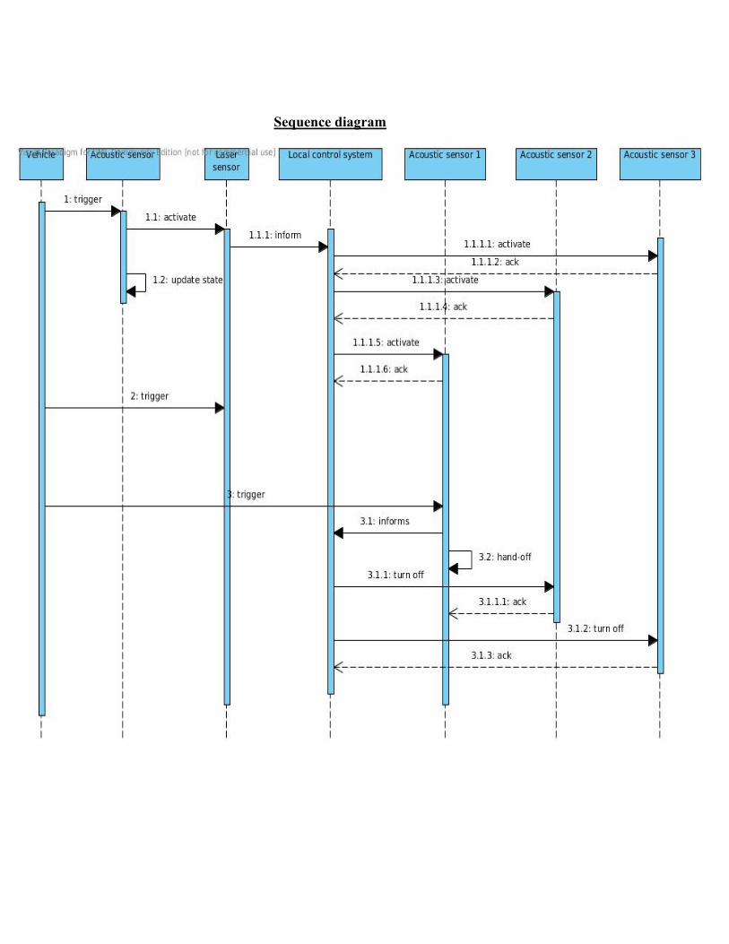
Sequence diagram

Use Case4. Straight line-Acoustic sensors communication Pre-conditions: Vehicle(s) starts moving along a straight road. First acoustic sensor is activated. Actors: Vehicle Flow of Events:

1. Activated sensor identifies the vehicle. 2. Sensor activates its neighbor and sends information which vehicle to expect 3. Sensor sends message to control system in order to update vehicle position. 4. Sensor removes plate of vehicle from its stack. 5. If stack empty sensor goes to idle state, else waits the other vehicle(s).

Post-conditions: Basic Flow: Vehicle arrives at an intersection or a parking lot or exit. Related parts of structure: the central control system, a node that has an acoustic sensor.

Activity diagram

Sequence diagram

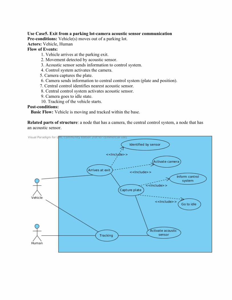
Use Case5. Exit from a parking lot-camera acoustic sensor communication Pre-conditions: Vehicle(s) moves out of a parking lot. Actors: Vehicle, Human Flow of Events:

1. Vehicle arrives at the parking exit. 2. Movement detected by acoustic sensor. 3. Acoustic sensor sends information to control system. 4. Control system activates the camera.

5. Camera captures the plate. 6. Camera sends information to central control system (plate and position).

7. Central control identifies nearest acoustic sensor. 8. Central control system activates acoustic sensor. 9. Camera goes to idle state. 10. Tracking of the vehicle starts.

Post-conditions: Basic Flow: Vehicle is moving and tracked within the base. Related parts of structure: a node that has a camera, the central control system, a node that has an acoustic sensor.

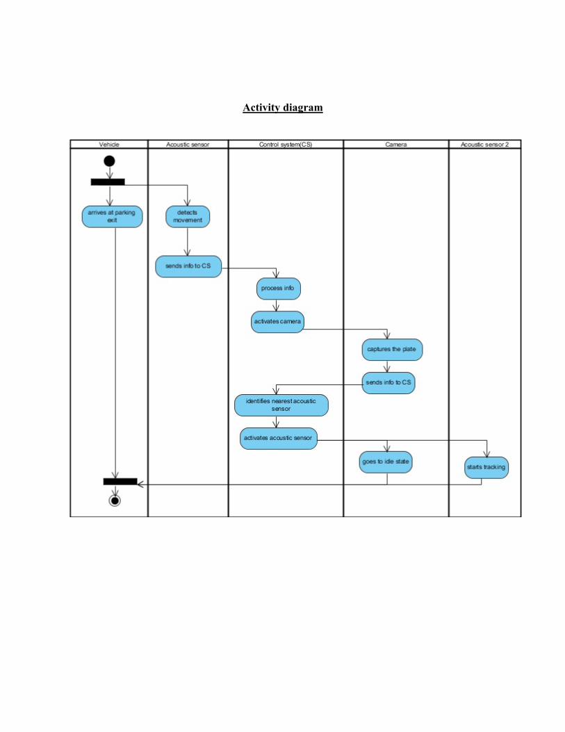
Activity diagram

Sequence diagram

Use Case6. Entry in a parking lot. Pre-conditions: Vehicle arrives at a parking lot. Actors: Vehicle Flow of Events:

1. Acoustic sensor at the entry of the parking lot identifies vehicle. 2. Acoustic sensor sends plate and position information to the central control system.

3. Central control system checks if vehicle is authorized to enter the parking. Post-conditions: Basic Flow: Vehicle inside the parking lot. State of the alarm (on/off). Related parts of structure: a node that has a camera, the central control system, a node that has an acoustic sensor.

Activity diagram

Sequence diagram

Use Case7. Acoustic sensor battery low Pre-conditions: Acoustic sensor is operating. Actors: Flow of Events: 1. Sensor detects battery level is low.

2. Sensor informs central control system. 3. Sensor is turned off. 4. Central control system sends information to previous sensor to update neighbor information. (previous acoustic sensor makes the next working sensor its neighbor)

Post-conditions: Basic Flow: System operates. Acoustic node needs maintenance.

Related parts of structure: the central control system, a node that has an acoustic sensor.

State machine diagrams

Acoustic sensor

Camera sensor

Part 3: Requirements

1. The system should be Energy efficient

-The number of the sensors should be such in order to optimize energy efficiency, cost and detection probability.

-Sensors should have different states.(off, idle, on)

2. The system should be accurate in detection and communication

- The sensing range of the acoustic sensor should be limited to one lane of the road. (use a reverse shotgun polar diagram for the acoustic sensor- width: 4m).

- Assuming 40 miles per hour maximum vehicle velocity and distance between

acoustic sensors is d. The message from one sensor to the other should be transmitted in less than t < d/50 (there is also a margin of safety).

- We need the sensor network to have a 95% probability of detection. - The power of the antenna should be enough to allow communication between two

sensors. - The time response of the Central Control System to messages from the camera

should be less than t < d / 20 (d distance between the camera and the acoustic sensor).

- The CCS should be capable of responding on time to simultaneous requests . - System should work even if one or more acoustic sensors stops operating. - System could turn off a misoperating sensor. - System should adapt to weather changes.

3. The system should be cost efficient

- The number of sensors used in the system should be optimized with respect also to energy efficiency

4. Security - The messages should be encrypted. - The CCS should have methods to identify intrusions and prevent attacks.

The hierarchy of requirements and how they are verified through the elements of the structure are presented below:

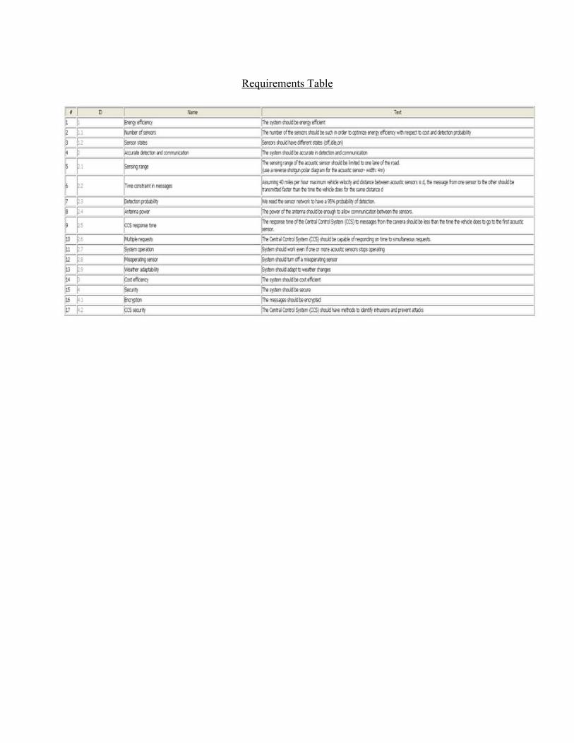
Requirements Table

 

 Derived  Requirements  

 

Requirement   Behavior   Structure  

     1.Energy  efficiency      1.1  Number  of  sensors     X  1.2  Node  states   X    2.  Accurate  detection  and  communication  

   

2.1  Sensing  range     X    2.2  Time  constraint  in  messages  

X    

2.3  Detection  and  tracking  probability  

X    

2.4  Antenna  power   X   X  2.5  CCS  response  time   X    2.6  Multiple  requests   X    2.7  System  operation   X    2.8  Misoperating  sensor   X    2.9  Weather  adaptability   X    3.  Cost  efficiency      4.  Security      4.1  Encryption   X    4.2  CCS  security   X   X          

Energy  efficiency,  Cost  efficiency,  Security,  Accurate  detection  and  Communication  are  the  system  level  Requirements.  

 

 

Traceability  Matrix  

  System  Components  Requirement   Object   Attribute   Function          1.Energy  efficiency   Sensor  Network      1.1  Number  of  sensors   Sensor  Network      1.2  Node  states   S_CPU  :  Node,    CCS   state  :  Node   Turn_on(),  Turn_off  ()    :  CCS  

Turn_on(),  Turn_off  ()    :  S_CPU  2.  Accurate  detection  and  communication  

Sensor  Network      

2.1  Sensing  range   Antenna:  Node   gain,    directivity,  position_X,  position_Y  :  Antenna  

 

2.2  Time  constraint  in  messages  

Channel   Length,    Message_time:  Channel     Transmit_message():  Channel  

2.3  Detection  and  tracking  probability  

Sensor  :  Node   Accuracy:  Sensor    

2.4  Antenna  power   Antenna:  Node  CCS_Antenna:  CSS  LCS_Antenna:  LCS  Channel  

Receiving  Power:  Antenna,  CCS_Antenna,  LCS_Antenna    Transmitting_Power:  Antenna,  CCS_Antenna,  LCS_Antenna    frequency:    Antenna,  CCS_Antenna,  LCS_Antenna    length:  Channel  

Transmit():  Antenna,  CCS_Antenna,  LCS_Antenna    Receive():  Antenna,  CCS_Antenna,  LCS_Antenna    Modulate():  Antenna,  CCS_Antenna,  LCS_Antenna  

2.5  CCS  response  time   CCS,  Channel   Response_time:  CCS  length:  Channel  

Process_message(),  Send_message()  :  CCS  

2.6  Multiple  requests   CCS   CPU,  RAM:  CCS    2.7  System  operation   Node     Report_status()  :  Node  2.8  Misoperating  sensor   CCS     Check_status:  CCS  2.9  Weather  adaptability   Antenna:  Node  

CCS_Antenna:  CSS  LCS_Antenna:  LCS  Channel  

modulation:    Antenna,  CCS_Antenna,  LCS_Antenna  weather:  Channel  

 

3.  Cost  efficiency   Sensor  Network   Cost:  Sensor  Network    4.  Security   Sensor  Network      4.1  Encryption   S_CPU(Node),  CCS,  LCS     Encrypt(),  Decrypt()  :    S_CPU,  CCS,  LCS  4.2  CCS  security   CCS     Operate_Honeypots():  CCS  

 

Explanation:      S_CPU  :  Node,  CCS    -­‐    means  that  the  object    S_CPU  of  the  Node  block  and  the  CCS  is  connected  with    the  requirement  

Abbreviations’  index:  

CCS:  Central  Control  System  

LCS:  Local  Control  System  

Part 4: Structure

Block Definition Diagram

Parametric Diagrams

The image cannot be displayed. Your computer may not have enough memory to open the image, or the image may have been corrupted. Restart your computer, and then open the file again. If the red x still appears, you may have to delete the image and then insert it again.

The image cannot be displayed. Your computer may not have enough memory to open the image, or the image may have been corrupted. Restart your computer, and then open the file again. If the red x still appears, you may have to delete the image and then insert it again.

The image cannot be displayed. Your computer may not have enough memory to open the image, or the image may have been corrupted. Restart your computer, and then open the file again. If the red x still appears, you may have to delete the image and then insert it again.

Part 5: Trade-Off Analysis:

System Performance Metrics:

-Accuracy

-Cost

-Energy Consumption

Decision Variables:

- Acoustic

-Laser Sensor

- Camera Sensor

- Central Control System

- Local Control System

Problem formulation:

For all functions that follow:

N1: The number of acoustic sensors.

N2: The number of laser sensors.

N3: The number of camera sensors.

N4: The number of local control systems.

-Cost = N1*C_X + N2*C_Y + N3*C_Z + N4*C_L+ C_C

C_X: The cost of one acoustic sensor.

C_Y: The cost of one laser sensor.

C_Z: The cost of one camera sensor.

C_L: The cost of one local control system.

C_C: The cost of the central control system.

-Accuracy: Because the malfunction of one sensor will affect the accuracy of the whole system, the following function can be used to measure the accuracy of the system.

Accuracy = R_X^N1 * R_Y^N2 * R_Z^N3 * R_L^N4 *R_C

R_X: The accuracy of one acoustic sensor.

R_Y: The accuracy of one laser sensor.

R_Z: The accuracy of one camera sensor.

R_L: The accuracy of one local control system.

R_C: The accuracy of the central control system.

To make the function, that is going to be used in CPLEX, linear, we take the log of the function, so our function will be:

-Accuracy = N1*log(R_X) + N2*log(R_Y) + N3*log(R_Z) + N4*log(R_L) + log(R_C)

-Energy Consumption = N1*P_X + N2*P_Y + N3*P_Z + N4*P_L + P_C

P_X: The power consumption of one acoustic sensor.

P_Y: The power consumption of one laser sensor.

P_Z: The power consumption of one camera sensor.

P_L: The power consumption of one local control system.

P_C: The power consumption of the central control system.

The power consumption of each sensor depends mainly on the power that the antenna needs for the transmission and receiving processes. Therefore, the following formula will be used to determine the energy consumption in each sensor node:

Energy Consumption = percentage_1*Rx + percentage_2*Tx + percentage_3*Pd,

Rx: The  current  consumption  for  transmission  mode  

Tx:    The  current  consumption  for  reception  mode  

Pd:  The  consumption  when  sensor  is  powered  down  

percentage_1:  The  percentage  of  time  the  sensor  is  on  Rx  mode

percentage_2:  The  percentage  of  time  the  sensor  is  on  Tx  mode

percentage_3:  The  percentage  of  time  the  sensor  is  on  Pd  mode

(Data are going to be acquired from datasheets and reviews on the internet)

Integer Programming Formulation:

For the trade off analysis three alternatives will be used for each of the decision variables.

•  Selection  of  the  acoustic  sensors  is  represented  by  variables  X    

X i = 1 for only one value of i = 1, 2, and 3. Otherwise, X i = 0.

•  Selection  of  the  laser  sensor  is  represented  by  variables  Y    

Y i = 1 for only one value of i = 1, 2, and 3. Otherwise, Y i = 0.

•  Selection  of  the  camera  sensor  is  represented  by  variables  Z    

Z i = 1 for only one value of i = 1, 2, and 3. Otherwise, Z i = 0.

•  Selection  of  the  local  control  system  is  represented  by  variables  L    

L i = 1 for only one value of i = 1, 2, and 3. Otherwise, L i = 0.

• Selection of the central control system is represented by variables C

C i = 1 for only one value of i = 1, 2, and 3. Otherwise, C i = 0.

  Formula for System Cost:

Cost C = N1*C_AS1*X1 + N1*C_AS2*X2 + N1*C_AS3*X3 + N2*C_LS1*Y1 + N2*C_LS2*Y2 + N2*C_LS3*Y3 + N3*C_CS1*Z1 + N3*C_CS2*Z2 + N3*C_CS3*Z3 + N4*C_LCS1*L1 + N4*C_LCS2*L2 + N4*C_LCS3*L3 + C_CCS1*C1 + C_CCS2*C2 + C_CCS3*C3

Formula for Performance:

Accuracy R = N1*R_AS1*X1 + N1*R_AS2*X2 + N1*R_AS3*X3 + N2*R_LS1*Y1 + N2*R_LS2*Y2 + N2*R_LS3*Y3 + N3*R_CS1*Z1 + N3*R_CS2*Z2 + N3*R_CS3*Z3 + N4*R_LCS1*L1 + N4*R_LCS2*L2 + N4*R_LCS3*L3 + R_CCS1*C1 + R_CCS2*C2 + R_CCS3*C3

Formula for Energy Consumption:

Energy E = N1*E_AS1*X1 + N1*E_AS2*X2 + N1*E_AS3*X3 + N2*E_LS1*Y1 + N2*E_LS2*Y2 + N2*E_LS3*Y3 + N3*E_CS1*Z1 + N3*E_CS2*Z2 + N3*E_CS3*Z3 + N4*E_LCS1*L1 + N4*E_LCS2*L2 + N4*E_LCS3*L3 + E_CCS1*C1 + E_CCS2*C2 + E_CCS3*C3

 

Design Objective

• Minimize cost and energy consumption and maximize accuracy

Minimize:

Energy E = 50*0.6481*X1 + 50*0.7628*X2 + 50*1*X3 + 12*0.6378*Y1 + 12*0.8586*Y2 + 12*1*Y3 + 5*0.6015*Z1 + 5*0.8333*Z2 + 5*1*Z3 + 3*0.7143*L1 + 3*0.8095*L2 + 3*1*L3 + 0.6030*C1 + 0.7528*C2 + 1*C3

Subject to

• K<= 50*0.013333*X1 + 50*0.015833*X2 + 50*0.02*X3 + 12*0.011667*Y1 + 12*0.015*Y2+ 12*0.018333*Y3 + 5*0.015*Z1 + 5*0.018333*Z2 + 5*0.025*Z3 + 3*0.066667*L1 + 3*0.075*L2 + 3*0.083333*L3 + 0.5*C1 + 0.833333*C2 + 1*C3 <= 2

• L<= 50*0.9375*X1 + 50*0.9583333*X2 + 50*1*X3 + 12*0.94949494 *Y1 + 12*0.969697 *Y2 + 12*1*Y3 + 5*0.92857*Z1 + 5*0.95918*Z2 + 5*1*Z3 + 3*0.6*L1 + 3*0.8*L2 + 3*1*L3 + 0.666667*C1 + 0.8*C2 + 1*C3 <= 0

• X1 + X2 + X3 = 1 • Y1 + Y2 + Y3 = 1 • Z1 + Z2 + Z3 = 1 • L1 + L2 + L3 = 1 • C1 + C2 + C3 = 1

Bounds

• 0 <= X 1 <=1, 0 <= X 2 <=1, 0 <= X 3 <=1, 0 <= Y 1 <=1, 0 <= Y 2 <=1, 0 <= Y 3 <=1, 0 <= Z 1 <=1, 0 <= Z 2 <=1, 0 <= Z 3 <=1, 0 <= L 1 <=1, 0 <= L 2 <=1, 0 <= L 3 <=1, 0 <= C 1 <=1, 0 <= C 2 <=1, 0 <= C 3 <=1,

Value Constraints

• X1, X2, X3, Y1, Y2, Y3, Z1, Z2, Z3, L1, L2, L3, C1, C2, and C3 are integers.

 

 

 

We change the values of K and L to get the different points with various cost, reliability and performance.

The following table is the different combination of K and L

 Point  #   L   K  

1   -­‐54   1.6  2   -­‐53.5   1.6  

3   -­‐45   1.7  

4   -­‐40   1.7  5   -­‐39   1.8  

6   -­‐38   1.8  7   -­‐35   1.9  

8   -­‐33   1.9  

9   -­‐31   2  10   -­‐30   2  

11   -­‐29   2.1  12   -­‐27   2.1  

13   -­‐25   2.2  14   -­‐23   2.3  

15   -­‐20   2.3  

16   -­‐15   2.4  17   -­‐10   2.4  

18   -­‐5   2.5  

19   -­‐1   2.6  

Each combination of L and K corresponds to each set of solution variables.

 

 

 

 

 

 

 

 

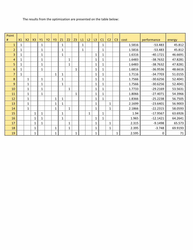
The  results  from  the  optimization  are  presented  on  the  table  below:  

 

Point  #   X1   X2   X3   Y1   Y2   Y3   Z1   Z2   Z3   L1   L2   L3   C1   C2   C3   cost   performance   energy  

1   1           1           1           1           1           1.5816   -­‐53.483   45.812  

2   1           1           1           1           1           1.5816   -­‐53.483   45.812  3   1           1           1                   1   1           1.6316   -­‐40.1721   46.6691  

4   1           1               1               1   1           1.6483   -­‐38.7632   47.8281  5   1           1               1               1   1           1.6483   -­‐38.7632   47.8281  

6   1           1                   1           1   1           1.6816   -­‐36.9536   48.6616  

7   1                   1   1                   1   1           1.7116   -­‐34.7703   51.0155  8       1       1           1                   1   1           1.7566   -­‐30.6256   52.4041  

9       1       1           1                   1   1           1.7566   -­‐30.6256   52.4041  10       1       1               1               1   1           1.7733   -­‐29.2169   53.5631  

11       1       1                   1           1   1           1.8066   -­‐27.4071   54.3966  

12       1               1   1                   1   1           1.8366   -­‐25.2238   56.7505  13       1               1   1                   1       1       2.1699   -­‐23.6401   56.9003  

14       1               1       1               1       1       2.1866   -­‐22.2315   58.0593  15           1   1           1               1       1           1.94   -­‐17.9567   63.6926  

16           1   1           1                   1   1           1.965   -­‐12.1421   64.2641  17           1   1               1               1       1       2.315   -­‐9.1498   65.573  

18           1           1       1               1       1       2.395   -­‐3.748   69.9193  

19           1           1           1           1           1   2.595   0   71    

 

 

 

 

 

 

 

 

 

 

Trade off Scenarios:

The  distribution  of  the  points  in  terms  of  “cost  vs  energy”,  “cost  vs  performance”,  and  “performance  vs  energy”  are  shown  in  the  following  charts,  some  of  the  points  overlap  because  some  different  combinations  of  K1  and  K2  produced  the  same  variable  values.  

 

Points of Interest:

Points  of  interest  are  adjacent  designs  where  an  incremental  increase  in  one  desirable  variable  creates  a  much  larger  increase  in  another  desirable  variable.  The  later  represents  a  point  that  will  be  studied  later  on,  to  determine  optimality  

Results:

Points  of  interest  that  are  common  to  all  three  graphs  are:  2,  6,  and  13  

Point  #   cost   performance   energy  

2   1.5816   -­‐53.483   45.812  

6   1.6816   -­‐36.9536   48.6616  13   2.1699   -­‐23.6401   56.9003  

 

Comparison  between  point  2  &  point  6:  

We  prefer  point  6  because  a  6%  increase  in  cost  and  energy  gives  us  a  30%  increase  in  performance.  

 

Comparison  between  point  6  &  point  13:  

We  prefer  point  13.    Although  it  costs  a  29%  increase  in  cost  and  a  17%  increase.    We  get  a  36%  increase  in  performance,  which  is  highly  desirable  especially  in  a  secured  military  base.  

 

FINAL RESULT

According to the analysis, the final choice is "point 13" which has best results for the given constraints.

• Attributes of Point 13 Cost = 2.1699, Energy = 56.9003, Performance = -23.6401

The de-normalized results of the analysis conclusion are as follows:

• Acoustic Sensor: Component AS2. • Laser Sensor: Component LS3. • Camera Sensor: Component CS1. • Local Control System: Component LCS 3. • Central Control System: Component CCS2.

The  system  total  cost  is  $13020.