Project planning with alternative technologies in ... · Project planning with alternative...
32
Project planning with alternative technologies in uncertain environments Creemers S, De Reyck B, Leus R. KBI_1314
-
Upload
duongkhuong -
Category
Documents
-
view
220 -
download
3
Transcript of Project planning with alternative technologies in ... · Project planning with alternative...

Project planning with alternative technologies in uncertain environments Creemers S, De Reyck B, Leus R.
KBI_1314

Project planning with alternative technologies in
uncertain environments
Stefan CreemersManagement Department
IESEG School of Management, Lille, France
Bert De ReyckDepartment of Management Science & Innovation
University College London, United Kingdom
Roel LeusResearch Group ORSTAT, Faculty of Economics and Business
KU Leuven, Belgium
— July 2013 —

Project planning with alternative technologies in
uncertain environments
Abstract: We investigate project scheduling with stochastic activity durations to maximize the expected
net present value. Individual activities also carry a risk of failure, which can cause the overall project
to fail. To mitigate the risk that an activity’s failure jeopardizes the entire project, more than one
alternative may exist for reaching the project’s objectives, and these alternatives can be implemented
either in parallel or in sequence. In the project planning literature, such technological uncertainty is
typically ignored and project plans are developed only for scenarios in which the project succeeds. We
propose a model that incorporates both the risk of activity failure and the possible pursuit of alternative
technologies. We find optimal solutions to the scheduling problem by means of stochastic dynamic
programming. Our algorithms prescribe which alternatives need to be explored, and whether they
should be investigated in parallel or in sequence. We also examine the impact of the variability of the
activity durations on the project’s value.
Managerial relevance: Project planning with traditional tools typically ignores technological and
duration uncertainty. We explain how to model scheduling decisions in a more practical environment
with considerable uncertainty, and we illustrate how decision making based only on expected values can
lead to inappropriate decisions. We also refute the intuition that an increase in uncertainty necessarily
entails a decrease of system performance, which seconds the proposal to focus also on ‘opportunity
management’ rather than only on ‘risk management.’
1 Introduction
Projects in many industries are subject to considerable uncertainty, due to many possible
causes. Factors influencing the completion date of a project include activities that are
required but that were not identified beforehand, activities taking longer than expected,
activities that need to be redone, resources being unavailable when required, late de-
liveries, etc. In research and development (R&D) projects, there is also the risk that
activities may fail altogether, requiring the project to be halted completely. This risk is
often referred to as technical risk. We focus on two main sources of uncertainty in R&D
projects, namely uncertain activity durations and the possibility of activity failure. We
examine the impact of these two factors on optimal planning strategies that maximize
the project’s value, and on its value itself.
We consider a single firm facing an R&D project with many possible development
patterns. The project is composed of a number of R&D activities with well-defined
1

precedence relationships, where each activity is characterized by a cost, a duration and
a probability of success. The successful completion of an activity can correspond to a
technological discovery or scientific breakthrough, for instance. To mitigate the risk that
an activity’s failure jeopardizes the entire project, the same outcome can be pursued in
several different ways, where one success allows the project to continue. The different
attempts can be multiple trials of the same procedure or the pursuit of different alternative
ways to achieve the same outcome, e.g., the exploration of alternative technologies. These
alternatives can be pursued either in parallel or sequentially, or following a mix of both
strategies, and management can also decide not to pursue certain alternatives, for instance
because their cost is too high compared to their expected benefits. Following Baldwin
and Clark [5], a unit of alternative interdependent tasks with a distinguished deliverable
will be called a module.
Project profitability is often measured by the project’s net present value (NPV), the
discounted value of the project’s cash flows. This NPV is affected by the project schedule
and therefore, the timing of expenditures and cash inflows has a major impact on the
project’s financial performance, especially in capital-intensive industries. The goal of this
paper is to find optimal scheduling strategies that maximize the expected NPV (eNPV)
of the project while taking into account the activity costs, the cash flows generated by
a successful project, the variability in the activity durations, the precedence constraints,
the likelihood of activity failure and the option to pursue multiple trials or technologies.
Thus, this paper extends the work of Buss and Rosenblatt [11], Benati [10], Sobel et
al. [45] and Creemers et al. [14], who focus on duration risk only, and of Schmidt and
Grossmann [44], Jain and Grossmann [26] and De Reyck and Leus [17], who look into
technical risk only (although Schmidt and Grossmann [44] also explore the possibility of
introducing multiple discrete duration scenarios). Our models are also related to those
of Nelson [39], Abernathy and Rosenbloom [1], Weitzman [50], Granot and Zuckerman
[23], Eppinger et al. [20], Krishnan et al. [27], Dahan [16], Loch et al. [31], Ding and
Eliashberg [18], Unluyurt [48], and Roemer and Ahmadi [43], who investigate the parallel
pursuit of alternative technologies in a variety of different settings.
Our contributions are fourfold: (1) we introduce and formulate a generic model for op-
timally scheduling R&D activities with stochastic durations, non-zero failure probabilities
and modular completion subject to precedence constraints; (2) we develop a dynamic-
programming recursion to determine an optimal policy for executing the project while
maximizing the project’s eNPV, extending the algorithm of Creemers et al. [14] with ac-
tivity failures, multiple trials and phase-type (PH) distributed activity durations instead
2
of exponentials; (3) we conduct numerical experiments to demonstrate the computational
capabilities of the algorithm; and (4) we examine the impact of activity duration risk on
the optimal scheduling policy and project values. Interestingly, our findings indicate that
higher operational variability does not always lead to lower project values, meaning that
(sometimes costly) variance reduction strategies are not always advisable.
The remainder of this text is organized as follows. Section 2 contains an overview
of related work. In Section 3, we provide the necessary definitions, leading to a de-
tailed problem statement in Section 4. We produce solutions by means of a backward
dynamic-programming recursion in a Markov decision chain, which is discussed in Sec-
tion 5. Section 6 reports on our computational performance on a representative set of
test instances. The effect of variability of activity durations on the eNPV of a project
is subsequently informally discussed by means of an illustration in Section 7. Section 8
contains a brief summary of the paper.
2 Related work
In the absence of resource constraints, the minimization of a project’s expected duration
is easily accomplished by starting each activity as soon as its predecessors are completed.
When the activity durations are stochastic, we are dealing with the so-called PERT
problem, for which most of the literature studies the computation of certain characteristics
of the minimum project makespan, mainly the exact computation, approximation and
bounding of its distribution function and expected value [2, 19, 28, 33].
In a deterministic setting, project scheduling to maximize NPV has already been
studied under a broad range of contractual arrangements and planning constraints (see
Herroelen et al. [24] for a review). Sobel et al. [45] extend these models to incorporate
stochastic activity durations and describe how to find the best policy from a finite set of
scheduling policies. A similar problem is studied by Benati [10], who proposes a heuristic
scheduling rule. Next to stochastic durations, Buss and Rosenblatt [11] also consider
activity delays.
We incorporate the concept of activity success or failure into the analysis of projects
with stochastic activity durations. De Reyck and Leus [17] develop an algorithm for
project scheduling with uncertain activity outcomes where all activity cash flows during
the development phase are negative, which is typical for R&D projects, and where project
success is achieved only if all individual activities succeed. Their work constitutes the first
description of an optimal approach for handling activity failures in project scheduling, but
3

neither stochastic activity durations nor the possibility of pursuing multiple alternatives
for the same result are accounted for. In that paper, if an activity A ends no later than
the start of another activity B then knowledge of the outcome (success or failure) of
A can sometimes be used to avoid incurring the cost for B, since a failure in A would
allow abandoning the project, but payment for B cannot be avoided when B has already
started before the outcome of A is discovered. For a given selection of such information
flows between activities (under the form of additional precedence constraints), a late-
start schedule is then optimal when the activity durations are known. The challenge,
of course, is to find the optimal set of information flows. Earlier papers have studied
optimal procedures for special cases; see Chun [12], for instance.
Unfortunately, late-start scheduling is difficult to implement in case of stochastic
durations, and Sobel et al. [45] implicitly restrict their attention to scheduling policies
that start activities only at the end of other activities. Buss and Rosenblatt [11] partially
relax this restriction by starting an activity only after a fixed time interval (delay), but
they do not decide which sets of activities to start at what time (all eligible activities are
started as soon as possible after their delay). Creemers et al. [14] study the same problem
as Sobel et al. [45] and achieve significant computational performance improvements. In
this article, we will also restrict our attention to policies that start activities at the
completion time of other activities. Finally, Coolen et al. [13] look into the properties of
different classes of scheduling policies for modular networks on a single machine; since no
discounting is applied, durations become irrelevant.
Other references relevant to this text stem from the discipline of chemical engineer-
ing, mainly the work by Grossmann and his colleagues (e.g., [44, 26]), who studied the
scheduling of failure-prone new-product development (NPD) testing tasks when non-
sequential testing is admitted. They point out that in industries such as chemicals and
pharmaceuticals, the failure of a single required environmental or safety test may prevent
a potential product from reaching the marketplace, which has inspired our modeling of
possible activity and project failure. Therefore, our models are also of particular interest
to drug-development projects, in which stringent scientific procedures have to be followed
in distinct stages to ensure patient safety, before a medicine can be approved for produc-
tion. Such projects may need to be terminated in any of these stages, either because the
product is revealed not to have the desired properties or because of harmful side effects.
Illustrations of modeling pharmaceutical projects, with a focus on resource allocation,
can be found in Gittins and Yu [22] and Yu and Gittins [51].
Due to the risk of activity failure resulting in overall project failure, it has been sug-
4

gested that R&D projects should explore multiple alternative ways for developing new
products (Sommer and Loch [46]). Thus, we include in our model alternative technologies
or multiple trials. Weitzman [50] identifies an optimal sequential scheduling strategy of
alternatives, each characterized by a cost, duration, and a reward probability distribu-
tion, which maximizes the expected present value. Weitzman’s Pandora’s rule is to select
the attempt with the highest reservation price (a measure that reflects each alternative’s
characteristics), to observe the stochastic outcome and to stop if the outcome is higher
than the reservation prices of all the remaining alternatives. Granot and Zuckerman [23]
examine the sequencing of R&D projects with success or failure in individual activities.
Like Weitzman [50], they only consider sequential stages, but they assume that each stage
is interrupted as soon one activity in that stage is successful. Nelson [39] and Abernathy
and Rosenbloom [1] demonstrate the value of scheduling alternative activities in paral-
lel. Nelson [39] aims to achieve a given objective at minimum cost. He characterizes
the optimal number of parallel development activities and shows that parallelism is most
beneficial when the cost of executing multiple alternatives is relatively small. Abernathy
and Rosenbloom [1] look at a case with two alternatives and show that while parallel exe-
cution is more expensive, it adds value by enabling a choice between the two technologies
if both are successful, and by fast-tracking the project in case one of the technologies
fails.
Dahan [16] examines the trade-off between parallel and sequential scheduling of alter-
native prototype development methods with Bernoulli outcomes. He explores the optimal
scheduling of homogeneous prototypes with identical characteristics and shows that for
high discount rates the optimal policy is a hybrid policy, whereas with low discount rates
a purely sequential policy is optimal. His analysis also demonstrates that extremely high
or low probabilities of technical success (PTS) reduce the variability of outcomes and
lead to fewer parallel prototypes being built.
Loch et al. [31] develop a dynamic-programming model to derive the optimal testing
strategy for design alternatives. Taking into account the testing cost, lead time, prior
knowledge and learning, they find that the optimal hybrid of parallel and sequential
testing depends on the ratio of cost and time, whereby parallel processing dominates
when the cost of delay increases relative to the cost of testing and development. Ding
and Eliashberg [18] examine a project portfolio pipeline in which multiple projects are
started simultaneously in order to increase the likelihood of having at least one successful
product. In the context of concurrent engineering, parallel versus sequential scheduling
of project activities has also been addressed, among others, by Eppinger et al. [20], Krish-
5
nan et al. [27] and Roemer and Ahmadi [43]. We refer to Lenfle [30] for a more extensive
literature review on parallel development strategies in project management, and to Bald-
win and Clark [5] for an elaborate description of the benefits of “modularity,” which
means splitting the design and production of technologies into independent subparts. In
this text, we will take the modular structure of the project as given, assuming that an
appropriate project network design has already been set out.
The idea of alternative work plans has recently also received attention in artificial
intelligence: Beck and Fox [8] suggest that there may be multiple alternative process
plans (routings) of an order through a factory, and they investigate how to incorporate
this issue into scheduling decisions. Bartak and Cepek [6] and Bartak et al. [7] continue
this work. In the literature on production management and automation, similar ideas of
alternative routings have been studied; see, for instance, Ahn et al. [3], Pan and Chen [42],
Nasr and Elsayed [38] and Kusiak and Finke [29]. To the best of our knowledge, however,
the literature on alternative process plans does not consider duration uncertainty nor the
possibility of activity failures.
The way in which we model project success in this paper is similar to the literature
on reliability systems, especially to the sequential testing of components of a multi-
component system in order to learn the state of the system when the tests are costly;
a comprehensive review of this area is provided in Unluyurt [48]. In these works, all
activities (tests) are performed in series and discounting is not considered; these two
characteristics actually go hand in hand, since it is a dominant decision to execute all
activities in series when money has no time value (see De Reyck and Leus [17]). In the
operational scheduling literature, different approaches to scheduling precedence-related
tasks with re-attempt at failure can be found in Mori and Tseng [37] and Malewicz
[34, 35].
3 Definitions
A project consists of a set of activities N = {0, . . . , n}. Some of these activities are
alternatives that pursue a similar target, representing repeated trials or technological
alternatives; such activities are gathered in one module. The set of modules is M =
{0, . . . ,m}; each module i ∈ M contains the activities Ni ⊂ N , and the set of modules
constitutes a partition of N : N =⋃i∈M Ni and Ni ∩ Nj = ∅ if i 6= j. Activities should
be executed without interruption. A is a (strict) partial order on M , i.e., an irreflexive
and transitive relation, which represents technological precedence constraints. (Dummy)
6

N0
4
N1 N2
N3
N4
6
5
0
1
2
3
Figure 1: Example module network
modules 0 and m represent the start and the end of the project, respectively; they are the
(unique) least and greatest element of the partially ordered set (M,A) and are assumed
to contain only one (dummy) activity, indexed by 0 and n, respectively. On the activities
within each module i, we also impose a partial order Bi, to allow for modeling precedence
requirements between these activities. Figure 1 illustrates these definitions. The project
consists of seven activities, N = {0, 1, 2, 3, 4, 5, 6}, where 0 and n = 6 are dummies.
There are five modules, so m = 4 : N0 = {0} , N1 = {1, 2, 3} , N2 = {4}, N3 = {5} and
N4 = {6}. In the example, B1 = {(1, 3), (2, 3)}. Note that Figure 1 actually shows the
transitive reduction of A: the order relation A also contains elements such as (0, 2) and
(1, 4), while the arcs N0 → N2 and N1 → N4 are not included in the figure.
Each activity i ∈ N\Nm has a PTS pi; we assume that p0 = 1. We do not consider
(renewable or other) resource constraints and assume the outcomes of the different tasks
to be independent. The cash flow associated with the execution of activity i ∈ N\Nm is
represented by the integer value ci and is incurred at the start of the activity. These ci
are usually non-positive, although the algorithm developed in Section 5 is able to handle
both positive and negative intermediate cash flows simultaneously. We choose c0 = 0. If
the project is successful, i.e., if every module is successful, it generates an end-of-project
payoff C ≥ 0, which is received at the start of activity n. A module is successful if at
least one of its constituent activities succeeds. Without loss of generality, we assume that
C is large enough for the project to be undertaken (otherwise, all starting times may be
set to infinity).
We define a success (state) vector as an n-component binary vector x = (x0, x1, . . . , xn−1),
with one component associated with each activity in N \ {n}. We let Xi represent the
Bernoulli random variable with parameter pi as success probability for each activity i, and
we write X = (X0, X1, . . . , Xn−1). Information on an activity’s success (the realization of
Xi) becomes available only at the end of that activity. We say that x is a realization or
scenario of X (the literature sometimes also uses the term random variate). The dura-
7

tion Dj ≥ 0 of each activity j is also a stochastic variable; the vector (D0, D1, . . . , Dn−1)
is denoted by D. We use lowercase vector d = (d0, d1, . . . , dn−1) to represent one par-
ticular realization of D, and we assume Pr[D0 = 0] = 1. For the remaining activities
j ∈ N \ {0, n}, the durations Dj are mutually independent PH-distributed stochastic
variables (see Section 5.3 for more details).
The value si ≥ 0 represents the starting time of activity i; we call the (n + 1)-vector
s = (s0, . . . , sn−1, sn) a schedule,with si ≥ 0 for all i ∈ N . We assume s0 = 0 in what
follows: the project starts at time zero. For convenience, we associate a completion time
ei(s; d,x) with each module i, in the following way (here and later, we omit the arguments
if no misinterpretation is possible): ei = min{+∞; minj∈Ni|xj=1{sj + dj}}. Clearly, if the
second min-operator optimizes over the empty set then ei = +∞, implying that the
module is never successfully completed. For a given success vector x and durations d, we
say that a schedule s is feasible if the following conditions are fulfilled:
ei ≤ sj ∀(i, k) ∈ A, ∀j ∈ Nk (1)
si + di ≤ sj ∀k ∈M,∀(i, j) ∈ Bk (2)
Equations (1) are inter-module precedence constraints, while Equations (2) are intra-
module constraints. An activity’s starting time equal to infinity corresponds to not
executing the activity and therefore not incurring any related expenses, or in case of
activity n, not receiving the project payoff. In words, the necessary conditions for the
start of an activity i ∈ Nj are (1) success for all the predecessor modules of the module j
to which i belongs, and (2) completion of all predecessor activities in the same module.
We compute the NPV for schedule s as
f(s) = Ce−rsn +n−1∑i=1
cie−rsi , (3)
with r a continuous discount rate chosen to represent the time value of money: the
present value of a cash flow c incurred at time t equals ce−rt. Here and below, we assume
e−0·∞ = 0. Note that symbol e is the base of the natural logarithm here, while above it
was used for module completion times; there will be little danger of confusion.
8
4 Problem statement
The execution of a project with stochastic components (in our case, stochastic activity
outcomes and durations) is a dynamic decision process. A solution, therefore, cannot be
represented by a schedule but takes the form of a policy : a set of decision rules defining
actions at decision times, which may depend on the prior outcomes. Decision times are
typically the start of the project and the completion times of activities; a tentative next
decision time can also be specified by the decision maker. An action entails the start of a
precedence-feasible set of activities (no constraints in (1) or (2) are violated). In this way,
a schedule is constructed gradually as time progresses. The following requirement, the
so-called non-anticipativity constraint, is also imposed: next to the information available
at the start of the project, a decision at time t can only use information on duration
realizations and realizations of components of X that has become available before or at
time t. The technical concept of a ‘policy’ corresponds to the practical notion of a project
strategy, which can be defined as a ‘direction’ in a project (goal, plan, guideline, . . . ) that
contributes to success of the project in its environment (Artto et al. [4]).
We follow Igelmund and Radermacher [25], Mohring [36] and Stork [47], who study
project scheduling with resource constraints and stochastic activity durations, in inter-
preting every policy Π as a function Rn≥ × Bn → Rn+1
≥ , with R≥ the set of non-negative
reals and B = {0, 1}. The function Π maps given samples (d,x) of activity durations
and success vectors to vectors s(d,x; Π) of feasible activity starting times (schedules).
For a given duration scenario d, success vector x and policy Π, sn(d,x; Π) denotes the
makespan of the schedule, which coincides with project completion. Note that not all
activities need to be completed (or even started) by sn, nor that the realization of all
Xi needs to be known. The earlier-mentioned PERT problem aims at characterizing the
random variable sn(D,1; ΠES), where policy ΠES starts all activities as early as pos-
sible, each module contains only one activity, and 1 is an n-vector with value 1 in all
components. Contrary to the makespan, however, NPV is a non-regular measure of per-
formance: starting activities as early as possible is not necessarily optimal, since the ci
may be negative.
Our goal is to select a policy Π∗ that maximizes E[f(s(D,X; Π))], with f(·) the NPV-
function as defined in Equation (3) and E[·] the expectation operator with respect to D
and X; we write E[f(Π)], for short. The generality of this problem statement suggests
that optimization over the class of all policies is probably computationally intractable.
We therefore restrict our optimization to a subclass that has a simple combinatorial
representation and where decision points are limited in number: our solution space P
9

consists of all policies that start activities only at the end of other activities (activity 0
is started at time 0).
For the example that was introduced in Section 3, a possible policy Π0 is the fol-
lowing: start the project at time 0 (s0 = 0) and immediately initiate activities 1 and 2
(s1 = s2 = 0). If X1 = X2 = 0 then abandon the project: set s3 = s4 = s5 = s6 = +∞.
Otherwise, module N1 completes successfully. In that case, start both activities 4 and 5
upon the successful completion of activity 1 or 2 (whichever is the earliest), and terminate
the project if either 4 or 5 fails. Note that under policy Π0, activity 3 is never started, and
we effectively include activity selection as part of the decisions to be made. Represented
as a function, Π0 entails the following mapping:
(d0, d1, d2, d3, d4, d5, x0, x1, x2, x3, x4, x5)
7→(0, 0, 0,∞, e1, e1,max{e2; e3}),
with e1 = min{d1 +∞ · (1 − x1); d2 +∞ · (1 − x2)}, e2 = e1 + d4 +∞ · (1 − x4) and
e3 = e1 + d5 +∞ · (1− x5). In the context of this article, we let 0 · ∞ = 0.
5 Markov decision chain
In the literature, the input parameters of the PERT problem are often referred as a PERT
network, and a PERT network with independent and exponentially distributed activity
durations is also called a Markovian PERT network. For Markovian PERT networks,
Kulkarni and Adlakha [28] describe an exact method for deriving the distribution and
moments of the earliest project completion time using continuous-time Markov chains
(CTMCs). Buss and Rosenblatt [11], Sobel et al. [45] and Creemers et al. [14] investigate
an eNPV objective and use the CTMC described by Kulkarni and Adklakha as a starting
point for their algorithms. These studies, however, assume success in all activities and
an exponential distribution for all durations and they also imply the requirement that all
activities be executed. In this article, we will extend the work of Creemers et al. [14] to
accommodate PH-distributed activity durations, possible activity failures and a modular
project network, allowing also for activity selection. Below, we first study the special case
of exponential activity durations (Section 5.1), followed by an illustration (Section 5.2)
and by a treatment of more general distributions (Section 5.3).
10
5.1 The exponential case
For the moment, we assume each duration Di to be exponentially distributed with rate
parameter λi = 1/E[Di] (i = 1, . . . , n − 1); we consider more general distributions in
Section 5.3. At any time instant t, an activity’s status is either idle (not yet started),
active (being executed), or past (successfully finished, failed, or considered redundant
because its module is completed). Let I(t), Y (t) and P (t) represent the activities in
N that are idle, active and past, respectively; these three sets are mutually exclusive
and I(t) ∪ Y (t) ∪ P (t) = N . The state of the system is defined by the status of the
individual activities and is represented by a triplet (I, Y, P ). State transitions take place
each time an activity becomes past and are determined by the policy at hand. The
project’s starting conditions are Y (0) = {0} and I(0) = N \ {0}, while the condition
for successful completion of the project is P (t∗) = N , where t∗ represents the project
completion time.
The problem of finding an optimal scheduling policy corresponds to optimizing a dis-
counted criterion in a continuous-time Markov decision chain (CTMDC) on the state
space Q, with Q containing all the states of the system that can be visited by the tran-
sitions (which are called feasible states); the decision set is described below. We apply a
backward stochastic dynamic-programming (SDP) recursion to determine optimal deci-
sions based on the CTMC described in Kulkarni and Adlakha [28]. The key instrument of
the SDP recursion is the value function F (·), which determines the expected NPV of each
feasible state at the time of entry of the state, conditional on the hypothesis that optimal
decisions are made in all subsequent states and assuming that all ‘past’ modules (with all
activities past) were successful. In the definition of the value function F (I, Y ), we supply
sets I and Y of idle and active activities as parameters (which uniquely determines the
past activities). When an activity finishes, three different state transitions can occur:
(1) activity j ∈ Ni completes successfully; (2) activity j ∈ Ni fails and another activity
k ∈ Ni is still idle or active; (3) activity j ∈ Ni fails and all other activities k ∈ Ni have
already failed (or it is the only activity in the module).
We define the order B∗ on set N to relate activities that do not necessarily belong to
the same module, as follows:
(i, j) ∈ B∗ ⇔ (∃Bm : (i, j) ∈ Bm) ∨ (∃(l,m) ∈ A : i ∈ Nl ∧ j ∈ Nm).
We call an activity j eligible at time t if j ∈ I(t) and ∀(k, j) ∈ B∗ : k ∈ P (t). Let
E(I, Y ) ⊂ N be the set of eligible activities for given sets I and Y of idle and active
11

activities. Upon entry of a state (I, Y, P ) ∈ Q, a decision needs to be made whether or
not to start eligible activities in E(I, Y ) and if so, which. If no activities are started, a
transition towards another state occurs at the first completion of an element of Y . Not
starting any activities while there are no active activities left, corresponds to abandoning
the project. Let λ =∑
k∈Y λk. The probability that activity j ∈ Y completes first
among the active activities equals λj/λ (see Appendix 1). The expected time to the first
completion is λ−1 time units (the length of this timespan is also exponentially distributed)
and the appropriate discount factor to be applied for this timespan is λ/(r + λ
)(cfr.
appendix). In state (I, Y, P ) ∈ Q, the expected NPV to be obtained from the next state
on condition that no new activities are started equals
λ
r + λ
∑j∈Y
pjλj
λF (I \Ni, Y \Ni)+
λ
r + λ
∑j∈Y :Ni\{j}6⊂P
(1− pj)λjλ
F (I, Y \ {j}),(4)
with j ∈ Ni in the summations. Our side conditions are F (I,∅) = 0 for all I.
The second alternative is to start a non-empty set of eligible activities S ⊆ E(I, Y )
when a state (I, Y, P ) ∈ Q is entered. This leads to incurring a cost∑
j∈S cj and an
immediate transition to another state, with no discounting required. The corresponding
eNPV, conditional on set S 6= ∅ being started, is
F (I \ S, Y ∪ S) +∑j∈S
cj. (5)
The total number of decisions S that can be made is 2|E(I,Y )|. The decision corresponding
to the highest value in (4) and (5) determines F (I, Y ).
The backward SDP recursion starts in state (∅, {n}, N \ {n}). Subsequently, the
value function is computed stepwise for all other states. The optimal objective value
maxΠ∈P E[f(Π)] is obtained as F (N \ {0}, {0}). We should note that the policies from
which one with the best objective function is chosen, do not consider the option of
starting activities at the end of activities that are redundant (past) because another
activity already made their module succeed.
12

Table 1: Project data for the example project
task i cash flow ci mean duration E[Di] PTS pi0 0 0 100%1 −20 10 40%2 −35 2 35%3 −70 8 75%4 −10 2 100%5 −10 2 60%6 0 100%
5.2 Illustration
In this section, we illustrate the functioning of the SDP algorithm by analyzing the
example project with seven activities (n = 6) introduced in Section 3, for which the
module order A is described by Figure 1. Further input data are provided in Table 1; the
project’s payoff value C is 300 and the discount rate is 10 percent per time unit (r = 0.1).
For exponentially distributed activity durations, the SDP recursion described in Sec-
tion 5.1 can be applied to find an optimal policy. At the onset of the project (in state
(N \ {0},∅, {0})) we can decide to start either the first activity, the second activity, or
both, from module 1. The SDP recursion evaluates the expected outcome of each of these
decisions and selects one that yields the highest expected NPV (assuming that optimal
decisions are made at all future decision times). In our example, it is optimal to start only
the first activity (corresponding to an objective function of 3.27) and we subsequently end
up in state ({2, 3, 4, 5}, {1}, {0}), in which two possibilities arise. If activity 1 succeeds,
module 1 succeeds as well and a transition occurs to state ({4, 5},∅, {0, 1, 2, 3}); otherwise
(if activity 1 fails), we end up in state ({2, 3, 4, 5},∅, {0, 1}) and have to make a decision:
either we start activity 2, corresponding to a transition to state ({3, 4, 5}, {2}, {0, 1})and an eNPV at that time for the remainder of the project of −1.06, or we abandon the
project altogether obtaining a current value of 0. The optimal decision in this case is
obviously not to continue the project.
After a successful completion of module 1, two new activities become eligible. The
optimal decision is to start both activities 4 and 5, leading to state (∅, {4, 5}, {0, 1, 2, 3}).Two possibilities then arise: either activity 4 or activity 5 finishes first. Irrespective of
which activity completes first, if either activity 4 or 5 fails then the entire project fails. If
activity 4 (resp. 5) finishes first and succeeds, activity 5 (resp. 4) is still in progress and
needs to finish successfully for the project payoff to be earned. We refer to this optimal
policy for exponential durations by the name Π1.
13

-1.06
-5.55
3.27
{1}
{1,2}
{2}
{2}
{4}
{4,5}
0.00
-1.06
success (1)
116.36
success (4)
success (5)
300.0
0.00
0.00
106.67
{5}110.00
success (5)
success (4)
fail (4)
fail (5)
fail (1)
Decision node
Chance node
Dominated decision
{ j } Decision to start activity j
Project
abandonment
D4>D
5
D4<D5
fail (5)
fail (4)
Figure 2: Optimal paths in the decision tree for the example project
The relevant part of the corresponding decision tree is represented in Figure 2, in
which the project evolves from left to right. A decision node, represented by a square,
indicates that a decision needs to be made at that point in the process; a chance node,
denoted by a circle, indicates that a random event takes place. Underneath each decision
node, we indicate the eNPV conditional on an optimal decision being made in the node,
which applies only to the part of the project that remains to be performed. For each
decision node, a double dash // is added to each branch that does not correspond to an
optimal choice in the SDP recursion.
5.3 Generalization towards PH distributions
PH distributions were first introduced by Neuts [40] as a means to approximate general
distributions using a combination of exponentials. We will adopt so-called acyclic PH
distributions for the activity durations in order to assess the impact of activity duration
variability on the eNPV of a project. In this section, we informally describe PH distribu-
tions and show how to determine the optimal eNPV of a project when activity durations
are PH distributed. Formal definitions and a moment-matching approach that can used
to approximate an arbitrary distribution are included as Appendix 2 and Appendix 3.
Due to the properties of the acyclic PH distribution, each activity j 6= 0, n can be
seen as a sequence of zj phases where:
• each phase θju has an exponential duration with rate λju,
• each phase θju has a probability τju to be the initial phase when starting activity j,
• each phase θju is visited with a given probability πjvu when departing from another
phase θjv.
14
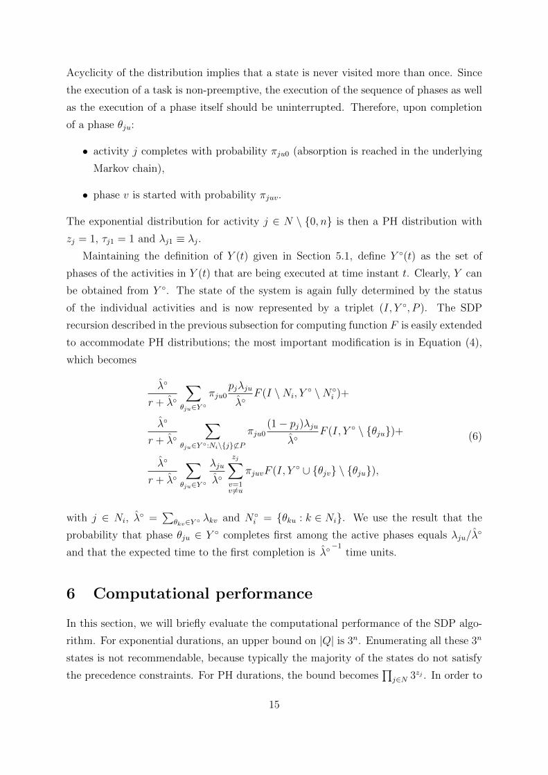
Acyclicity of the distribution implies that a state is never visited more than once. Since
the execution of a task is non-preemptive, the execution of the sequence of phases as well
as the execution of a phase itself should be uninterrupted. Therefore, upon completion
of a phase θju:
• activity j completes with probability πju0 (absorption is reached in the underlying
Markov chain),
• phase v is started with probability πjuv.
The exponential distribution for activity j ∈ N \ {0, n} is then a PH distribution with
zj = 1, τj1 = 1 and λj1 ≡ λj.
Maintaining the definition of Y (t) given in Section 5.1, define Y ◦(t) as the set of
phases of the activities in Y (t) that are being executed at time instant t. Clearly, Y can
be obtained from Y ◦. The state of the system is again fully determined by the status
of the individual activities and is now represented by a triplet (I, Y ◦, P ). The SDP
recursion described in the previous subsection for computing function F is easily extended
to accommodate PH distributions; the most important modification is in Equation (4),
which becomes
λ◦
r + λ◦
∑θju∈Y ◦
πju0pjλju
λ◦F (I \Ni, Y
◦ \N◦i )+
λ◦
r + λ◦
∑θju∈Y ◦:Ni\{j}6⊂P
πju0(1− pj)λju
λ◦F (I, Y ◦ \ {θju})+
λ◦
r + λ◦
∑θju∈Y ◦
λju
λ◦
zj∑v=1v 6=u
πjuvF (I, Y ◦ ∪ {θjv} \ {θju}),
(6)
with j ∈ Ni, λ◦ =
∑θkv∈Y ◦ λkv and N◦i = {θku : k ∈ Ni}. We use the result that the
probability that phase θju ∈ Y ◦ completes first among the active phases equals λju/λ◦
and that the expected time to the first completion is λ◦−1
time units.
6 Computational performance
In this section, we will briefly evaluate the computational performance of the SDP algo-
rithm. For exponential durations, an upper bound on |Q| is 3n. Enumerating all these 3n
states is not recommendable, because typically the majority of the states do not satisfy
the precedence constraints. For PH durations, the bound becomes∏
j∈N 3zj . In order to
15

minimize storage and computational requirements, we adopt the techniques proposed by
Creemers et al. [14]: as the algorithm progresses, the information on the earlier generated
states will no longer be required for further computation and therefore the memory occu-
pied can be freed. This procedure is based on a partition of Q, allowing for the necessary
subsets to be generated and deleted when appropriate.
We borrow the datasets that were generated by Coolen et al. [13]: these consist of
10 instances for each of various values of the number of activities n and for OS = 0.4,
0.6 and 0.8, with ‘order strength’ OS the number of comparable activity pairs according
to the induced order B∗, divided by the maximum possible number of such pairs (this
value is only approximate). Average activity durations are not used by Coolen et al. [13]
and are additionally generated for each activity, for each instance separately; each such
average duration is a uniform integer random variate between 1 and 15. The sign of the
cash flows is unimportant to our algorithm; in the generated instances, all activities apart
from the final one have negative cash flows.
In our implementation, storage requirement for 600, 000 states amounts to a maximum
of 4.58 MB; we only generate feasible states. Our experiments are performed on an AMD
Phenom II with 3.21 GHz CPU speed and 2, 048 MB of RAM. Under this configuration,
a state space of maximum 268, 435, 456 states can be entirely stored in memory. Our
results are presented in Tables 2-4, gathered per combination of values for OS and n.
The tables show that networks of up to 40 activities are analyzed with relative ease.
When n = 51, however, the optimal solution of most networks with low order strength
(OS = 0.4) is beyond reach when the system memory is restricted to 2, 048 MB. When
OS = 0.6, the performance is limited to networks with n = 71 or less. We observe that
the density of the induced order B∗ is a major determinant for the computational effort:
order strengths and computation times clearly display an inverse relation.
7 Impact of activity duration variability
In this section, we examine the impact of different degrees of variability of the activity
durations for the example project instance. The policy Π1 described in Section 5.2 is
optimal with exponential durations; its objective value is 3.27. The quality of the policy
changes when the variability level is different, however. Figure 3(a) illustrates the func-
tioning of policy Π1 with deterministic durations: the policy first executes only activity 1,
and then starts both activity 4 and 5 if 1 succeeds, otherwise the project is abandoned.
16
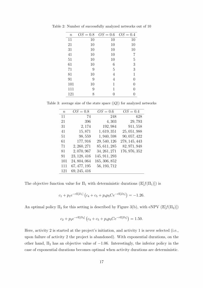
Table 2: Number of successfully analyzed networks out of 10
n OS = 0.8 OS = 0.6 OS = 0.411 10 10 1021 10 10 1031 10 10 1041 10 10 751 10 10 561 10 6 371 9 5 381 10 4 191 9 4 0101 10 1 0111 9 1 0121 8 0 0
Table 3: average size of the state space (|Q|) for analyzed networks
n OS = 0.8 OS = 0.6 OS = 0.411 74 248 62821 396 4, 303 29, 79331 2, 174 192, 984 911, 55841 15, 871 1, 619, 351 25, 051, 98851 98, 559 1, 940, 598 90, 057, 42261 177, 916 29, 540, 126 278, 145, 44371 2, 260, 271 85, 611, 285 82, 971, 94881 2, 070, 967 34, 261, 271 176, 976, 35291 23, 128, 416 145, 911, 293101 24, 804, 064 165, 306, 852111 67, 477, 195 56, 193, 712121 69, 245, 416
The objective function value for Π1 with deterministic durations (E[f(Π1)]) is
c1 + p1e−rE[D1]
(c4 + c5 + p4p5Ce
−rE[D5])
= −1.26.
An optimal policy Π2 for this setting is described by Figure 3(b), with eNPV (E[f(Π2)])
c2 + p2e−rE[D2]
(c4 + c5 + p4p5Ce
−rE[D5])
= 1.50.
Here, activity 2 is started at the project’s initiation, and activity 1 is never selected (i.e.,
upon failure of activity 2 the project is abandoned). With exponential durations, on the
other hand, Π2 has an objective value of −1.06. Interestingly, the inferior policy in the
case of exponential durations becomes optimal when activity durations are deterministic.
17

Table 4: average CPU time required to find an optimal policy
n OS = 0.8 OS = 0.6 OS = 0.411 0 0 021 0 0 0.0331 0 0.3 1.7741 0.02 3.54 70.9351 0.15 5.12 298.4161 0.32 128.31 2, 397.9371 17.53 469.34 27, 065.5381 5.7 1817.54 15, 605.9191 107.61 1, 322.77101 105.66 894.61111 283.57 10, 540.86121 528.81
0 1 2 3 4 5 6 7 8 9 10 11 12 13 Time10
11 12 13 Time10
1-20
0Project
abandonment
300
5-10
4-10100%
60%
40%
60%
(a) Policy Π1
0 1 2 3 4 5 Time2
3 4 5 Time2
2-35
0Project
abandonment
300
5-10
4-10100%
60%
35%
65%
(b) Policy Π2
Figure 3: Policies with deterministic durations
Also, the effect of variability on the eNPV associated with a policy is not monotonic;
the eNPV of policy 1 increases, whereas the eNPV of policy 2 decreases. Of particular
interest is the fact that the eNPV can actually increase when variability is introduced,
which is quite counterintuitive. Note also that for each of the two variability settings, the
sign of the objective of two policies is different (one policy achieves a negative NPV while
the other one has positive NPV). This is a strong case for incorporating all variability
information into the computations and not only ‘plugging in’ the expectations into a
deterministic model, since a good project might be cut from the portfolio based only
expected values, whereas it would be able to add value with a carefully selected scheduling
strategy.
To investigate the impact of variability in more detail, we use PH distributions to
model the activity durations, which will allow us to increase or decrease the variability
and examine its impact on the project’s eNPV, by changing the Squared Coefficient of
Variation (SCV) of the activity durations (for simplicity, we assume all activity durations
to have equal SCV). Setting SCV equal to 1 corresponds to exponentially distributed
18
0 0.2 0.4 0.6 0.8 1 1.2 1.4 1.6 1.8 2−2
0
2
4
6
Squared coefficient of variation of activity durations
eN
PV
of th
e e
xam
ple
pro
ject
Policy Π1
(a) effect on eNPV of policy Π1
0 0.2 0.4 0.6 0.8 1 1.2 1.4 1.6 1.8 2−2
0
2
4
6
Squared coefficient of variation of activity durations
eN
PV
of th
e e
xam
ple
pro
ject
Policy Π2
(b) effect on eNPV of policy Π2
0 0.2 0.4 0.6 0.8 1 1.2 1.4 1.6 1.8 2−2
0
2
4
6
Squared coefficient of variation of activity durations
eN
PV
of th
e e
xam
ple
pro
ject
Optimal policy
Policy Π1
Policy Π2
(c) effect on optimal eNPV
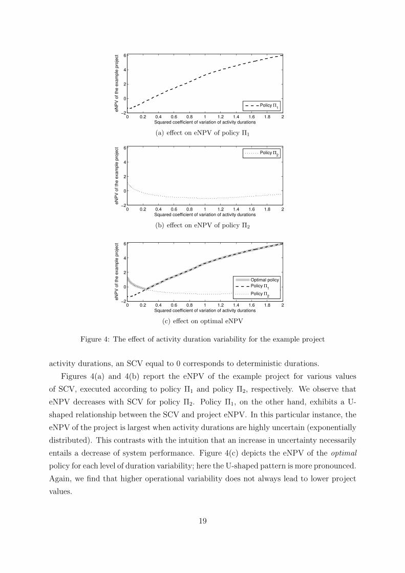
Figure 4: The effect of activity duration variability for the example project
activity durations, an SCV equal to 0 corresponds to deterministic durations.
Figures 4(a) and 4(b) report the eNPV of the example project for various values
of SCV, executed according to policy Π1 and policy Π2, respectively. We observe that
eNPV decreases with SCV for policy Π2. Policy Π1, on the other hand, exhibits a U-
shaped relationship between the SCV and project eNPV. In this particular instance, the
eNPV of the project is largest when activity durations are highly uncertain (exponentially
distributed). This contrasts with the intuition that an increase in uncertainty necessarily
entails a decrease of system performance. Figure 4(c) depicts the eNPV of the optimal
policy for each level of duration variability; here the U-shaped pattern is more pronounced.
Again, we find that higher operational variability does not always lead to lower project
values.
19

Ward and Chapman [49] argue that all current project risk-management processes
induce a restricted focus on the management of project uncertainty. In part, this is
because the term ‘risk’ encourages a ‘threat’ perspective: we refer the reader to the ex-
amples of risk events in the model for variability reduction by Ben-David and Raz [9] and
Gerchack [21]. Ward and Chapman state that a focus on ‘uncertainty’ rather than risk
could enhance project risk management, providing an important difference in perspective,
including, but not limited to, an enhanced focus on opportunity management, an ‘oppor-
tunity’ being a ‘potential welcome effect on project performance.’ Ward and Chapman
suggest that management strive for a shift from a threat focus towards greater concern
with understanding and managing all sources of uncertainty, with both up-side and down-
side consequences, and explore and understand the origins of uncertainty before seeking
to manage it. They suggest using the term ‘uncertainty management,’ encompassing
both ‘risk management’ and ‘opportunity management.’ The suggestions of Ward and
Chapman are seconded from an operational viewpoint by our computational results. See
also Loch et al. [32] for examples of how downside risks can sometimes be turned into
upside opportunity (e.g., p. 5 and p. 20).
8 Summary and conclusions
In this article, we have developed a generic model for the optimal scheduling of R&D-
project activities with stochastic durations, non-zero failure probabilities and multiple
trials subject to precedence constraints. We assess the effect of different degrees of ac-
tivity duration variability on the expected NPV of a project. We illustrate that higher
operational variability does not always lead to lower project values, meaning that (some-
times costly) variance reduction strategies are not always advisable.
Appendix 1 Some technical results used in Section 5.1
Suppose that Xi ∼ Exp(λi) for i = 1, . . . , ω, so the cdf of Xi is FXi(t) = 1 − e−λit, and
that the Xi are independent. It then holds that Y = mini=1,...,ω{Xi} is also exponential,
with rate∑
i λi. This can be seen as follows:
20

FY (t) = Pr[Y ≤ t] = 1− Pr[Y > t]
= 1− Pr[X1 > t] · . . . · Pr[Xω > t]
= 1− e−λ1t · . . . · e−λωt
= 1− exp
(−t∑i
λi
),
which we recognize as the cdf of an exponential variable with the mentioned rate.
The following is a classic result known as that of ‘competing exponentials’:
Pr[k = arg mini=1,...,ω
{Xi}] =λk∑i λi
.
For ω = 2, we have
Pr[X1 ≤ X2] =
∫ ∞0
∫ ∞t1
λ1e−λ1t1λ2e
−λ2t2dt2dt1
=
∫ ∞0
λ1e−λ1t1e−λ2t1dt1
= λ1
∫ ∞0
e−(λ1+λ2)t1dt1
=λ1
λ1 + λ2
∫ ∞0
e−udu =λ1
λ1 + λ2
.
These integrals generalize straightforwardly to compute Pr[(Xk ≤ X1)∧(Xk ≤ X2)∧ . . .].In a very similar way, the appropriate discount factor in expectation, with continuous
per-unit discount rate r over the timespan Y = mini=1,...,ω{Xi}, can be obtained as
follows. We determine the present value e−rY of a cash flow of 1 at time Y . Above, we
have already established the distribution of Y . We obtain
∫ ∞0
e−rt
(∑i
λi
)e−(
∑i λi)tdt = . . . =
∑i λi
r +∑
i λi.
One might argue that these computations are insufficient for application in Section 5
because the cash flow to be discounted actually depends on which of the Xi is the smallest.
We now show that this does not preclude the foregoing simple result from being applied.
21
Define the function
ζ(X1, X2, . . . , Xω) =c1 if X1 ≤ X2, X1 ≤ X3, . . .,
c2 if X2 < X1 and X2 ≤ X3, X2 ≤ X4, . . .,...
cω if Xω < X1, Xω < X2, . . ..
We wish to determine the expected discounted value of ζ. We find∫ ∞0
c1e−rt1 .λ1e
−λ1t1 .e−∑
i 6=1 λit1dt1+∫ ∞0
c2e−rt2 .λ2e
−λ2t2 .e−∑
i 6=2 λit2dt2+
. . .∫ ∞0
cωe−rtω .λωe
−λωtω .e−∑
i6=ω λitωdtω
=λ1c1
r +∑
i λi+
λ2c2
r +∑
i λi+ . . .+
λωcωr +
∑i λi
=
( ∑i λi
r +∑
i λi
)(λ1∑i λi
c1 + . . .+λω∑i λi
cω
).
The first term of the right-hand side of the final line of these equations is exactly the
discount factor that we already obtained, while the second term is the expectation
E[ζ(X1, . . . , Xn)] of ζ without discounting. In other words, we can separate the com-
putation of the expected value and the application of the discounting factor.
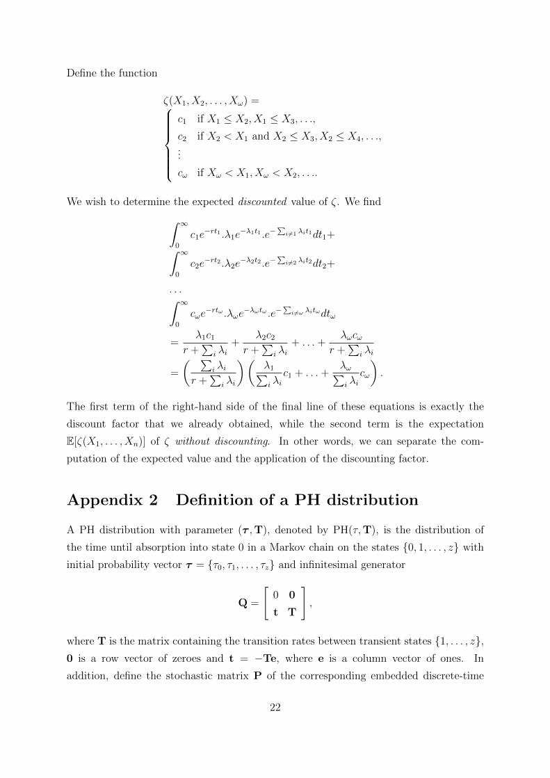
Appendix 2 Definition of a PH distribution
A PH distribution with parameter (τ ,T), denoted by PH(τ,T), is the distribution of
the time until absorption into state 0 in a Markov chain on the states {0, 1, . . . , z} with
initial probability vector τ = {τ0, τ1, . . . , τz} and infinitesimal generator
Q =
[0 0
t T
],
where T is the matrix containing the transition rates between transient states {1, . . . , z},0 is a row vector of zeroes and t = −Te, where e is a column vector of ones. In
addition, define the stochastic matrix P of the corresponding embedded discrete-time
22

Markov chain. Let πuv and quv denote the vth entry of the uth row of the embedded
Markov chain P and the infinitesimal generator Q, respectively. The entries of P are
computed as follows:
πuv =
− quvquu
if u > 0 ∧ u 6= v,
1 if u = 0 ∧ v = 0,
0 otherwise.
We will consider only acyclic PH distributions, in which each state is never visited
more than once in the Markov chain whose absorption time defines the PH distribution.
Examples of acyclic PH distributions include: the exponential, the Erlang, the hypo-
exponential, the hyper-exponential and the Coxian distribution (Osogami [41]). Note
that for acyclic PH distributions, it is possible to index the statespace such that T is an
upper-triangular matrix.
In this article, we distinguish three PH distributions: (1) the exponential distribution;
(2) the hypo-exponential distribution; and (3) the two-phase Coxian distribution. An
exponential distribution with rate parameter λ is an acyclic PH distribution with initial
probability vector τ = {0, 1} and infinitesimal generator
Q =
[0 0
λ −λ
].
The exponential distribution itself is the simplest of PH distributions. An Erlang dis-
tribution is the convolution of z exponentials that have identical rate parameter λ.
The corresponding acyclic PH distribution has z phases, initial probability vector τ =
{0, 1, 0, . . . , 0} and infinitesimal generator
Q =
0 0 0 . . . 0 0
0 −λ λ . . . 0 0
0 0 −λ . . . 0 0
· · · · · · · · · · · · · · · · · ·0 0 0 . . . −λ λ
λ 0 0 . . . 0 −λ
.
A hypo-exponential distribution or generalized Erlang distribution is the convolution of
z exponential distributions with possibly different rate parameters. The corresponding
acyclic PH distribution has z phases, initial probability vector τ = {0, 1, 0, . . . , 0} and
23

infinitesimal generator
Q =
0 0 0 . . . 0 0
0 −λ1 λ1 . . . 0 0
0 0 −λ2 . . . 0 0
· · · · · · · · · · · · · · · · · ·0 0 0 . . . −λz−1 λz−1
λz 0 0 . . . 0 −λz
.
A two-phase Coxian distribution is a mixture of two exponential distributions and corre-
sponds to an acyclic PH distribution that has initial probability vector τ = {0, 1, 0} and
infinitesimal generator
Q =
0 0 0
(1− β)λ1 −λ1 βλ1
λ2 0 −λ2
.A transition is made from the first phase towards the second phase with probability β.
If the second phase is not visited (with probability 1 − β), absorption takes place after
visiting the first phase.
Appendix 3 Moment matching
Let λ−1 and σ2 denote the mean and variance of a random variable X, respectively. The
squared coefficient of variation of X is ϕ2 = σ2λ2. We describe the two-moment matching
procedure described in Creemers et al. [15] that allows to determine the parameters of
the PH distribution that matches the mean and the variance of X.
We distinguish three cases. The first case is ϕ < 1; then a hypo-exponential can be
used to model X’s distribution, with the following parameters:
z = dϕ−2e,
λz =1 +
√(z − 1) (zϕ2 − 1)
λ (1− zϕ2 + ϕ2),
λu =(z − 1)−
√(z − 1) (zϕ2 − 1)
λ (1− ϕ2),
for all u ∈ {1, 2, . . . , z − 1}. The initial probability vector of the corresponding PH
24

distribution is defined as follows:
τu =
{1 if u = 1,
0 otherwise.
Alternatively, ϕ > 1 and X can be modeled via a two-phase Coxian distribution with
parameters
τ0 = 0,
τ1 = 1,
τ2 = 0,
β =2 (κ− 1)2
1 + ϕ2 − 2κ,
λ1 =λ
κ,
λ2 =2λ (κ− 1)
2κ− 1− ϕ2,
where κ is a value that can be chosen to determine the expected duration of the first
phase. In this article we assume κ = 0.5.
The third case is ϕ = 1 and X is then approximated by an exponential distribution,
so
τ0 = 0,
τ1 = 1,
λ1 = λ.
References
[1] W. J. Abernathy and R. S. Rosenbloom, “Parallel strategies in development projects,”
Manage. Sci., vol. 15, no. 10, pp. 486–505, 1969.
[2] V. G. Adlakha and V. G. Kulkarni, “A classified bibliography of research on stochastic
PERT networks,” INFOR, vol. 27, no. 3, pp. 272–296, 1989.
[3] J. Ahn, W. He, and A. Kusiak, “Scheduling with alternative operations,” IEEE Trans.
Robot. Autom., vol. 9, no. 3, pp. 297–303, 1993.
25

[4] K. Artto, J. Kujala, P. Dietrich, and M. Martinsuo, “What is project strategy?,” Int.
J. Project Manage., vol. 26, no. 1, pp. 4–12, 2008.
[5] C. Y. Baldwin and K. B. Clark, Design Rules: The Power of Modularity. Cambridge,
MA, USA: The MIT Press, 2000.
[6] R. Bartak and O. Cepek, “Temporal networks with alternatives: Complexity and
model,” in Proc. Twentieth Int. Florida Artificial Intell. Res. Soc. Conf., D. Wilson
and G. Sutcliffe, Eds. Menlo Park, CA, USA: The AAAI Press, 2007, pp. 641–646.
[7] R. Bartak, O. Cepek, and M. Hejna, “Temporal reasoning in nested temporal net-
works with alternatives,” in Recent Advances in Constraints – 12th Annual ERCIM
International Workshop on Constraint Solving and Constraint Logic Programming,
CSCLP 2007 Rocquencourt, France, June 7-8, 2007 Revised Selected Papers, F. Fages,
F. Rossi, and S. Soliman, Eds. Germany: Springer-Verlag Berlin Heidelberg, 2008,
pp. 17–31.
[8] J. C. Beck and M. S. Fox, “Constraint-directed techniques for scheduling alternative
activities,” Artificial Intell., vol. 121, pp. 211–250, 2000.
[9] I. Ben-David and T. Raz, “An integrated approach for risk response development in
project planning,” J. Oper. Res. Soc., vol. 52, no. 1, pp. 14–25, 2001.
[10] S. Benati, “An optimization model for stochastic project networks with cash flows,”
Computational Manage. Sci., vol. 3, no. 4, pp. 271–284, 2006.
[11] A. H. Buss and M. J. Rosenblatt, “Activity delay in stochastic project networks,”
Oper. Res., vol. 45, no. 1, pp. 126–139, 1997.
[12] Y. H. Chun, “Sequential decisions under uncertainty in the R&D project selection
problem,” IEEE Trans. Eng. Manag., vol. 41, no. 4, pp. 404–413, 1994.
[13] K. Coolen, W. Wei, F. Talla Nobibon, and R. Leus, “Scheduling modular projects
on a bottleneck resource,” J. Sched., to appear, DOI 10.1007/s10951-012-0294-9.
[14] S. Creemers, R. Leus, and M. Lambrecht, “Scheduling Markovian PERT networks
to maximize the net present value,” Oper. Res. Lett., vol. 38, no. 1, pp. 51–56, 2010.
[15] S. Creemers, M. Defraeye, and I. Van Nieuwenhuyse, “A Markov model for measur-
ing service levels in nonstationary G(t)/G(t)/s(t)+G(t) queues,” KU Leuven, Faculty
of Business and Economics, Department of Decision Sciences and Information Man-
agement working paper #1306, 2013.
26

[16] E. Dahan, “Reducing technical uncertainty in product and process development
through parallel design of prototypes,” Stanford University, Graduate School of Busi-
ness working paper, 1998.
[17] B. De Reyck and R. Leus, “R&D-project scheduling when activities may fail,” IIE
Trans., vol. 40, no. 4, pp. 367–384, 2008.
[18] M. Ding and J. Eliashberg, “Structuring the new product development pipeline,”
Manage. Sci., vol. 48, no. 3, pp. 343–363, 2002.
[19] S. Elmaghraby, Activity Networks: Project Planning and Control by Network Models,
New York, NY, USA: John Wiley & Sons Inc, 1977.
[20] S. D. Eppinger, D. E. Whitney, R. P. Smith, and D. A. Gebala, “A model-based
method for organizing tasks in product development,” Res. Eng. Des., vol. 6, no. 1,
pp. 1–13, 1994.
[21] Y. Gerchak, “On the allocation of uncertainty-reduction effort to minimize total
variability,” IIE Trans., vol. 32, no. 5, pp. 403–407, 2000.
[22] J. Gittins and J. Y. Yu, “Software for managing the risks and improving the prof-
itability of pharmaceutical research,” Int. J. Technol. Intell. Planning, vol. 3, no. 4,
pp. 305–316, 2007.
[23] D. Granot and D. Zuckerman, “Optimal sequencing and resource allocation in re-
search and development projects,” Manage. Sci., vol. 37, no. 2, pp. 140–156, 1991.
[24] W. S. Herroelen, P. Van Dommelen, and E.L. Demeulemeester, “Project network
models with discounted cash flows: A guided tour through recent developments,”
Eur. J. Oper. Res., vol. 100, no. 1, pp. 97–121, 1997.
[25] G. Igelmund and F. J. Radermacher, “Preselective strategies for the optimization of
stochastic project networks under resource constraints,” Networks, vol. 13, no. 1, pp.
1–28, 1983.
[26] V. Jain and I. E. Grossmann, “Resource-constrained scheduling of tests in new prod-
uct development,” Ind. and Eng. Chemistry Res., vol. 38, no. 8, pp. 3013–3026, 1999.
[27] V. Krishnan, S. D. Eppinger, and D. E. Whitney, “A model-based framework to
overlap product development activities,” Manage. Sci., vol. 43, no. 4, pp. 437–451,
1997.
27

[28] V. Kulkarni and V. Adlakha, “Markov and Markov-regenerative PERT networks,”
Oper. Res., vol. 34, no. 5, pp. 769–781, 1986.
[29] A. Kusiak and G. Finke, “Selection of process plans in automated manufacturing
systems,” IEEE Trans. Robot. Autom., vol. 4, no. 4, pp. 397–402, 1988.
[30] L. Lenfle, “The strategy of parallel approaches in projects with unforeseeable uncer-
tainty: The Manhattan case in retrospect,” Int. J. Project Manage., vol. 29, no. 4,
pp. 359–373, 2011.
[31] C. H. Loch, C. Terwiesch, and S. Thomke, “Parallel and sequential testing of design
alternatives,” Manage. Sci., vol. 47, no. 5, pp. 663–678, 2001.
[32] C. H. Loch, A. DeMeyer, and M. T. Pich, Managing the Unknown: A New Approach
to Managing High Uncertainty and Risk in Projects. Hoboken, NJ, USA: Wiley,
2006.
[33] A. Ludwig, R. M. Mohring, and F. Stork, “A computational study on bounding the
makespan distribution in stochastic project networks,” Ann. Oper. Res., vol. 102, pp.
49–64, 2001.
[34] G. Malewicz, “Parallel scheduling of complex dags under uncertainty,” in Proc. Sev-
enteenth Annu. ACM Symp. Parallelism algorithms architectures. New York, NY,
USA: ACM, 2005, pp. 66–75.
[35] G. Malewicz, “Implementation and experiments with an algorithm for parallel
scheduling of complex dags under uncertainty,” in Proceedings of the Eighth Work-
shop on Algorithm Engineering and Experiments and the Third Workshop on Analytic
Algorithmics and Combinatorics (Proceedings in Applied Mathematics), R. Raman,
R. Sedgewick, and M. F. Stallmann, Eds. Miami, FL, USA: SIAM, 2006, pp. 66–74.
[36] R. H. Mohring, “Scheduling under uncertainty: Optimizing against a randomizing
adversary,” Lecture Notes Comput. Sci., vol. 1913, pp. 15–26, 2000.
[37] M. Mori and C. C. Tseng, “A resource constrained project scheduling problem with
reattempt at failure: A heuristic approach,” J. Oper. Res. Soc. Japan, vol. 40, no. 1,
pp. 33–44, 1997.
[38] N. Nasr and E. A. Elsayed, “Job shop scheduling with alternative machines,” Int.
J. Prod. Res., vol. 28, no. 5, pp. 1595–1609, 1990.
28

[39] R. R. Nelson, “Uncertainty, learning, and the economics of parallel research and
development efforts,” Rev. Econ. Stat., vol. 43, no. 4, pp. 351–364, 1961.
[40] M. F. Neuts, Matrix-Geometric Solutions in Stochastic Models. Baltimore, MD,
USA: Johns Hopkins University Press, 1981.
[41] T. Osogami, “Analysis of multiserver systems via dimensionality reduction of Markov
chains,” Carnegie Mellon University, Computer Science Department, PhD Thesis,
2005.
[42] C. H. Pan and J. S. Chen, “Scheduling alternative operations in two-machine flow-
shops,” J. Oper. Res. Soc., vol. 48, no. 5, pp. 533–540, 1997.
[43] T. A. Roemer and R. Ahmadi, “Concurrent crashing and overlapping in product
development,” Oper. Res., vol. 52, no. 4, pp. 606–622, 2004.
[44] C. W. Schmidt and I. E. Grossmann, “Optimization models for the scheduling of
testing tasks in new product development,” Ind. Eng. Chemistry Res., vol. 35, no. 10,
pp. 3498–3510, 1996.
[45] M. J. Sobel, J. G. Szmerekovsky, and V. Tilson, “Scheduling projects with stochastic
activity duration to maximize expected net present value,” Eur. J. Oper. Res., vol.
198, no. 1, pp. 697–705, 2009.
[46] S. C. Sommer and C. H. Loch, “Selectionism and learning in projects with complexity
and unforeseeable uncertainty,” Manage. Sci., vol. 50, no. 10, pp. 1334–1347, 2004.
[47] F. Stork, “Stochastic resource-constrained project scheduling,” Technische Univer-
sitat Berlin, PhD Thesis, 2001.
[48] T. Unluyurt, “Sequential testing of complex systems: A review,” Discrete Appl.
Math., vol. 142, pp. 189–205, 2004.
[49] S. Ward and C. Chapman, “Transforming project risk management into project
uncertainty management,” Int. J. Project Manage., vol. 21, pp. 97–105, 2003.
[50] M. L. Weitzman, “Optimal search for the best alternative,” Econometrica, vol. 47,
no. 3, pp. 641–654, 1979.
[51] J. Y. Yu and J. Gittins, “Models and software for improving the profitability of
pharmaceutical research,” Eur. J. Oper. Res., vol. 189, no. 2, pp. 459–475, 2008.
29

FACULTY OF ECONOMICS AND BUSINESS Naamsestraat 69 bus 3500
3000 LEUVEN, BELGIË tel. + 32 16 32 66 12 fax + 32 16 32 67 91
[email protected] www.econ.kuleuven.be