Project M4, M9 and F6 Final Report July 2008 CRC Enabling Technologies Heather A. Sheldon pmd*CRC...
98
pmd*CRC Project M4, M9 and F6 Final Report July 2008 Enabling Technologies Compiled by Heather A. Sheldon
Transcript of Project M4, M9 and F6 Final Report July 2008 CRC Enabling Technologies Heather A. Sheldon pmd*CRC...

pm
d*CRCEnabling Technologies
Heather A
. Sheldon
pmd*CRCProject M4, M9 and F6 Final Report July 2008 Enabling Technologies
Compiled by Heather A. Sheldon
M4, M
9 and F6 Final Report
pmd*CRCProject M4, M9 and F6 Final Report July 2008 Enabling Technologies
Compiled by Heather A. SheldonCSIRO Exploration & Mining
Core Partners
Sponsors

Page 3
pmd*CRC ProjeCtS M4, M9 and F6 Final rePort
ContributorS
James S. Cleverley, Soazig Corbel, Andy Dent, Gordon W. German, Bruce E. Hobbs, Peter Hornby, Alison Ord, Warren Potma, Klaus Regenauer-Lieb, Thomas Poulet, Peter Schaubs, Heather A. Sheldon, Yanhua Zhang (CSIRO Exploration & Mining, PO Box 1130, Bentley, WA 6102)
Paul A. Roberts (Predictive Discovery Pty Ltd, c/o CSIRO Exploration & Mining, PO Box 1130, Bentley, WA 6102)
Evgeniy Bastrakov, Richard Chopping, Terry Mernagh, Dale Percival, Yuri Shvarov (Onshore Energy and Minerals Division, Geoscience Australia, GPO Box 378, Canberra, ACT 2601)
Carsten Laukamp (School of Earth and Environmental Sciences, James Cook University, Townsville, Qld 4811)
Page 4
ContentS
Executive summary 6
Part 1 – Overview 7
1.1 Advances in the Application of Enabling Technologies to Mineral Exploration Since the Start of the pmd*CRC 7
1.2 Computational Utilities for Predictive Mineral Discovery: Seven Years of Effort 11
1.3 Application of Numerical Modelling Technologies to Predictive Exploration Targeting 12
1.4 Advances in Understanding of Hydrothermal ore Systems, Crustal Fluid Flow and Mechanics during the pmd*CRC 14
Part 2 – Technical details and deliverables 27
2.1 The Desktop Modelling Toolkit 27
2.2 Advances in 3D Mesh Construction 30
2.3 The Reactive Transport Utility 38
2.4 Validating Heat and Tracer Transport in the Reactive Transport Utility 45
2.5 Coupling Reactive Transport with Deformation 49
2.6 Virtual Centre for Geofluids 53
2.7 Modified Cam Clay: A Constitutive Model for Simulating Deformation of Porous Rocks 58
2.8 Damage Mechanics and Stress Transfer Modelling: A Technique for Predicting Permeability Evolution in and Around Faults 61
2.9 Modelling Magmatic and Metamorphic Fluid Production in Flac3D 64
2.10 Conditions for Free Convection in the Earth’s Crust 69
2.11 Modelling Deformation with Particle Codes 76
2.12 Reactive Transport Modelling 79
2.13 Using Reactive Transport Models to Predict the Geophysical Responses of Alteration 85
2.14 Validation of Spectral Techniques for Exploration in the Mt Isa Terrane 89
2.15 A Thermodynamically Consistent Multi-scale Approach to Mineralising Systems 94
Part 3 – Publications
The following sections are available on the enclosed CD
Selected Application Case Studies (electronic)
A1.1 Deformation – fluid flow modelling examples
A1.1A Central Gawler Au province: Tunkillia deposit scale models
A1.1B Central Gawler Au province: Tunkillia 10 x 10 km models
A1.1C Central Gawler Au province: Tunkillia regional models
A1.1D Central Gawler Au province: Tarcoola models (including HCh geochemical models)
A1.1E Mt Pleasant Quarters Deposit
A1.1F Kanowna Bell
A1.1G Wallaby 2D and 3D
A1.2 Heat – fluid flow modelling example: Central Gawler Au province: Regional heat + fluid flow models
A1.3 RT modelling example: Uranium RT models (PIRSA)
A1.4 Thermo-mechanical Modelling of High Temperature Deformation (I7 project)
A1.5 Numerical Modelling of the Leichhardt River Fault Trough (I7 project)
A1.6 3D models of coupled Deformation, Heat and Fluid Flow in the Mt Isa Inlier (I7 project)
A1.7 Discrete Element (UDEC) modelling in the Mt Isa Inlier (I7 project)
Appendix 2 – Supporting documents (electronic)
Sheldon_Micklethwaite_2007.pdf
Sheldon_Micklethwaite_2007_supplementaryMaterial.pdf
Sheldon_Micklethwaite_AGU_2006.pdf
Sheldon_Micklethwaite_AGU_2006.ppt
Twiki_ProjectM9StressTransferDamage.zip
COULOMB_data.zip
STMtoVTK.zip
Viscoelastic_damage_Hamiel.zip
Twiki_CamClayInitialPorosityDepth.zip
Twiki_CamClayExtension.zip

Page 5
pmd*CRC ProjeCtS M4, M9 and F6 Final rePort
Twiki_CamClayUnitTests.zip
CamClayDLL.zip
CamClayModelFiles.zip
Barnicoat_Sheldon_STOMP_2005.ppt
pmdCRC_conference_2006_camclay_poster.ppt
Sheldon_EGU_2005.pdf
Sheldon_EGU_2005.ppt
Sheldon_et_al_2006.pdf
Sheldon_et_al_STOMP_2005.pdf
RajitGoel_CamClay_Project.zip
RajitGoel_CamClay_models.zip
mag_met_fluids_FLAC3D.zip
Twiki_ProjectM9Convection.zip
Twiki_ProjectM9ConvectionNotes.zip
Sheldon_Fermor_2006.ppt
Sheldon_Fermor_abstract_2006.pdf
pmdPyRT_transport_benchmarking.doc
pmdPyRT_benchmark_python.zip
pmdPyRT_benchmark_meshes.zip
Advancements_in_Mesh_Construction_-_Appendix.doc
Enabling Technology Conference Abstracts
Page 6
pmd*CRC ProjeCtS M4, M9 and F6 Final rePort
exeCutive SuMMary
This report summarises the outcomes of the Modelling and Fluids programs of the Predictive Mineral Discovery Cooperative Research Centre (pmd*CRC), specifically projects M4, M9 and F6. The aims of these projects were:
M4: Ensure relevant data collected during the pmd*CRC research program, and knowledge and information derived from these data, are readily accessible to the CRC’s clients and partners.
M9: Deliver a combination of knowledge, data, technology, know-how and skilled personnel to provide a new predictive targeting strategy to the global exploration industry.
F6: Apply and develop predictive geochemical technologies and methods, focusing on refinement and delivery of tools developed in earlier phases of the pmd*CRC.
Part 1 gives an overview of the new technologies that have been developed, their application to predictive mineral discovery, and consequent advances in understanding of hydrothermal ore systems. Part 2 offers detailed information on specific technology products, including the Desktop Modelling Toolkit, mesh construction methods, the Reactive Transport Modelling utility, and the Virtual Centre for Geofluids (incorporating FreeGs and FIncs). It also includes reports on theoretical developments and emerging technologies, including spectral methods, damage mechanics, the use of particle codes for modelling brittle rock behaviour, and prediction of geophysical signatures from reactive transport models. Some methods in Part 2 have yet to be applied to mineral exploration but will provide a foundation for modelling tools of the future. Examples of the application of numerical modelling to mineral systems are presented in Appendix 1, in the form of four-page pamphlets and reports. Appendix 2 contains supporting documents, such as conference abstracts and presentations, and code to run some of the examples presented in other parts of the report.

Page 7
pmd*CRC ProjeCtS M4, M9 and F6 Final rePort
Part 1 – overview
Factors hindering the applicability of numerical modelling tools to mineral exploration-problems at the CRC’s start were:
• Inefficiencyofthemodellingprocess(resultinginnumerical modelling research projects typically running for many months or years to achieve useful outcomes);
• Alimitedrangeofdeposittypesandgeologicalprocesses to which the technology could be effectively applied; and
• Alackofknowledgeofthetechnologyamongexploration geologists and postgraduate researchers.
All of this meant that there was no practical way to use these tools in routine mineral exploration. The CRC’s research program aimed to:
• Improvetheefficiencyofthenumericalmodellingworkflow so problems could be addressed in weeks or months rather than years;
• Widentherangeofgeologicalproblemsandoresystemsthat numerical modelling could address; and
• Undertakeexemplarprojectsanddevelopeducationalmaterial to increase the profile of numerical modelling in the mineral exploration and economic geology research community.
Progress in these areas during the CRC is described below. The CRC’s numerical modelling and fluids programs have left a huge legacy including:
• Apurpose-builtnumericalmodellingtoolkitdesignedfor exploration targeting problems which is more efficientthananyothercomparablecapabilityinthe world;
• Alargeteamofnumericalmodellerswiththecapabilityto provide numerical modelling services for exploration targeting within Australia as well as making scientific advances in this research domain;
• Asubstantialpublishedrecordofimprovementsinthe application of numerical modelling to geological processes in mineral systems;
• Manycasehistoriesoftheapplicationofnumericalmodelling to mineral targeting problems; and
• Abigresourceofeducationalmaterial.
1.1 Advances in the Application of Enabling Technologies to Mineral Exploration Since the Start of the pmd*CRC
Paul A. Roberts
Introduction
The pmd*CRC ’s numerical modelling and fluids programs were designed to support the CRC’s goal of generating a paradigm shift in the mineral exploration industry’s targeting approach, enabling the industry to move from empirical to process-oriented targeting methods.
The industry’s unfavourable view of process-driven targeting at the start of the CRC arose from experiences of poor discovery outcomes from the use of such “conceptual” approaches. It was believed this problem could be solved if the validity of targeting concepts based on geological processthinkingcouldbereadilyandefficientlytestedby“experiments”. The CRC focused on numerical modelling as an experimental tool because it is the only tool that can reproduce the physical conditions, spatial scales and time frames relevant to mineralisation. Numerical modelling enables geologists to experiment with geological parameters in order to identify scenarios in which mineralisation is likely to form. These parameters include geometry, fluid and rock chemistry, temperature, stress field orientation, pore fluid pressure, porosity and permeability.
At the start of the CRC, no exploration company was using numerical modelling routinely in its targeting methodology. Dr Peter Holyland had offered a numerical modelling service to the industry in the 1990’s, using Itasca’s UDEC code, but this was not available when the CRC began. Since the 1980’s, CSIRO and university researchers in Australia and overseas have used numerical modelling in research projects to investigate hydrothermal ore formation. The CRC’s modelling and fluids programs were the first well-funded attempt in the world to make numerical modelling a standard component in the mineral exploration industry’s toolkit.

Page 8
meshes (i.e. meshes in which the number of cells along each axis is maintained throughout the model) for geometries defined by intersecting planar or curved surfaces, and to vary the mesh geometry simply by changing a few characters in a text file. The templates have been useful for exploring simple geometric problems (e.g. the effect of varying strike and dip of intersecting faults) and as a teaching aid.
• AsuiteofgOcad2 “wizards” was developed to enable users to build meshes for certain classes of geometry without needing extensive gOcad experience.
• TechniquesforcreatingstructuredmeshesingOcadfrom imported triangulated surfaces.
• Techniquesformeshingcomplexgeometriesthatinclude wedges and other shapes (e.g. intrusive bodies) not easily subdivided into hexahedra. The modelling team has experimented with a variety of mesh building tools and gained benefit from using PATRAN3.
These techniques have enabled the modelling team to build meshes with a level of geological complexity and fidelity to interpreted geological surfaces that was unknown at the CRC’s outset.
Running models
The most significant development in this area was the Desktop Modelling Toolkit (DMT). This enables users to run various numerical modelling codes on a choice of hardware platforms (local or remote). Resultant benefits include:
• Muchoperatingknowledge(includingalargeamountof CRC-developed code for Flac3D) is embedded in the DMT, enabling users with less intensive knowledge of the underlying codes to run them successfully (note: operating the software remains the domain of expert users because strong knowledge of the underlying science and the strengths and weaknesses of numerical modelling in the geosciences is needed).
• TheDMTenablesuserstochooseappropriatecomputing resources for a problem. For example, users can run a suite of tens or hundreds of models on a remote super computer to explore the effects of varying geometries and parameter values. Alternatively, the user
2 gOcad: www.pdgm.com/gocad-base-module/products.aspx 3 PATRAN: www.mscsoftware.com/products/patran.cfm
While the CRC has not yet provided the spur for a wholesale change in exploration practice in Australia, they have left a legacy that will enable that change in future.
Improving modelling efficiency
The workflow of numerical modelling consists of:
1. Mineral system analysis;
2. Identifying a series of testable geological problems;
3. Constructing geological geometries and converting them into meshes suitable for numerical modelling;
4. Running models, typically involving multiple versions of the same model with varying geometries and/or parameter values;
5. Visualisation of model results;
6. Interpretation.
Steps 1, 2 and 6 involve geological analysis. The CRC’s existence has enabled a large team of modelling practitioners to work on a wide range of mineral exploration projects, leading to significant improvements intheteam’sefficiencyandskillsingeologicalanalysis.
Research efforts in the modelling program aimed to radicallyimproveefficiencyinsteps3,4and5.Aspecificobjective of the modelling program was to improve efficienciesbytwoordersofmagnitudeduringtheCRC’slife. This outcome is hard to demonstrate but it is clear that theefficiencyofmodellingwiththesoftwareusedovertheCRC’s life – namely Flac3D (Itasca Consulting Group, 2002) and HCh (Shvarov and Bastrakov, 1999) – has improved by at least 10 times, and in some cases 100 times.
Meshing
Mesh construction is a time-consuming step in the numerical modelling workflow, especially for geomechanical modelling codes such as Flac3D1 which require meshes composed of hexahedral elements. Improvements made include:
• Aseriesofmesh-buildingtemplatesweredevelopedforuse with Flac3D. They enable users to build “structured”
1 Flac3D: www.itascacg.com/flac3d/index.html

Page 9
pmd*CRC ProjeCtS M4, M9 and F6 Final rePort
Reactive transport code
An important development in the numerical modelling and fluids program has been a new reactive transport (RT) code which enables coupled simulation of fluid flow, thermal evolution, solute transport and chemical reaction along with the resultant changes in porosity and permeability. Results can be produced relatively rapidly (by the standards of reactive transport modelling) in complex geometries with realistic chemistries, and over sensible model time periods (e.g. 1 million years). The code is capable of operating in 3D but the computational cost of running it in 3D on realistic geometries combined with realistic chemistries and time scales is prohibitive. The key stumbling block is the slowness of the chemical solver which can only be run on Windows. Alternative strategies for chemical calculations will continue to be investigated after the CRC ends.
A novel application of the RT code is the prediction of geophysical signatures of alteration systems. This approach is useful for detecting mineralisation and alteration under cover. The CRC has developed algorithms to convert the evolving alteration mineralogies from RT models into density and magnetic susceptibility numbers for each mesh element. This enables forward modelling of the effects of alteration systems on detectable geophysical signals, a capability which has never been available before.
Four-fold coupling
An important aim of the CRC’s numerical modelling program was to develop a robust code for modelling of the four-fold coupled system (i.e. deformation, fluid flow, thermal evolution and chemical reactions). Significant progress was made but application of such a tool to a realistic example was not achieved before the CRC ended.
Work on four-fold coupling was in progress at the CRC’s start using the 3DMACS prototype code. Various problems with the coupling component were encountered, including the stability and accuracy of the reactive transport calculations. A complete re-write of the RT code took precedence over four-fold coupling developments for most of the CRC’s life.
Effort was re-focused on this problem in the CRC’s final two years. Stable results have been achieved in simple experiments using the commercial finite element code
may choose to run the model on their own desktop machine or on an unused machine elsewhere in the same building.
The DMT builds on other efforts in CSIRO, including the 3DMACS code-coupling prototype tool which was in development at the CRC’s start, and a big effort by the CSIRO Computational Geoscience group on grid computing under the national SEEGRID and Auscope initiatives.
Visualisation
Visualisation of model results has become a significant bottleneck in the modelling workflow as the capacity to generate large numbers of models has increased. Important visualisation tools have included FracSIS4 and freeware tools such as MayaVi5. Early in the CRC’s life, CSIRO funded FracSIS developments which helped provide the functionality necessary for visualising numerical model outputs.
A major advance realised during the CRC was the development of the PIG (Productive Interactive Graphics) interface, designed for use with the HCh geochemical modelling code (Shvarov and Bastrakov, 1999). PIG improved the ability of CRC geochemists to visualise and interpret HCh model results. This was of particular benefit when working with industry geologists in field locations.
Widening the range of geological problems
The CRC’s modelling and fluids programs have made significant progress in:
• Reactivetransportcodedevelopment;
• Developmentofafour-foldcoupledsystemforsimultaneous simulation of deformation, fluid flow, thermal evolution and chemical reaction;
• Otheradvancesingeomechanics;and
• ApplicationofCRCcapabilitytoawideningrangeofore systems and scales.
These advances are discussed below.
4 FracSIS: www.fractaltechnologies.com/5 MayaVi: http://mayavi.sourceforge.net/
Page 10
• EpithermalgoldsystemsintheGreatBasin,Nevada.
The range of soluble problems has been expanded to include deformation and faulting in porous rocks; fluid flow through faults between sealed compartments; permeability evolution due to deformation and chemical reactions; and fluid production from metamorphism and cooling magmas.
Exemplar projects and educational materials
Exemplar projects
The CRC modelling and fluids teams have undertaken numerous targeting projects with client companies, both sponsors and non-sponsors of the CRC, investigating a variety of mineral systems across Australia and overseas. The pace of this activity increased enormously in the last 3 years of the CRC. Pamphlets describing research results were produced for many of these projects and distributed at meetings and conferences (subject to permission from the sponsors). Many projects have generated conclusions which have influenced the exploration strategies of sponsoring companies, with some resulting in discovery of mineralisation (e.g. Stawell, VIC).
Educational materials
An early CRC project developed a virtual “Modelling Library” which included information about the science and practice of numerical modelling illustrated by case histories. At the project’s end, this was made into a website.
The most significant educational activity, however, has been development of materials for courses. Many courses and workshops have been delivered in Australia and overseas during the CRC, starting in July 2002 as part of the University of WA’s Masters program and ending with a workshop in June 2008. In addition, substantial course material has been developed for graduate courses at the University of WA.
References
Itasca Consulting Group, 2002. Flac3D: Fast lagrangian analysis of continua in 3 dimensions. Itasca, Minneapolis.
Shvarov, Y.V. and Bastrakov, E.N. (Eds). 1999. HCh: A software package for geochemical equilibrium modelling. User’s guide. Australian Geological Survey Organisation, Canberra, Australia.
Abaqus6 for modelling deformation, coupled with the CRC’s RT code.
Other advances in geomechanics
An active geomechanics research program has operated throughout the CRC’s life. Much of the work focused on using existing capability to investigate poorly-understood geological phenomena. Other important research investigations have included:
• applicationofdamagemechanicstopermeabilityevolution and mineralisation around faults;
• applicationoftheCamClayconstitutivemodeltodeformation and permeability evolution in porous rocks;
• applicationofparticlecodestoexaminefractureformation at the grain scale, some magmatic processes and brecciation.
The research team has also benefited from contributions by Professors Klaus Regenauer-Lieb (WA Premier’s Fellow) and Bruce Hobbs (CSIRO Research Fellow). Of particular importance has been the publication of seminal papers recognising the importance of thermal-mechanical feedbacks in geological systems, which have led to a new understanding of rock strength and structure formation at and below the brittle-ductile transition.
Widening the range of ore systems and scales
The numerical modelling and fluids research teams have worked on a range of ore systems, from prospect to district scale, including:
• MesothermalgoldsystemsinWesternAustralia,Queensland, South Australia, New South Wales and Victoria.
• Unconformityandrollfronturaniumsystemsinthe Alligator River (Northern Territory) and Frome Embayment (SA) regions respectively.
• Sediment-hostedmassivesulphideandstructurally-controlled base metal systems in the Century area, Queensland and the Cobar District, New South Wales.
• Volcanic-hostedbasemetalmineralisationintheOutokumpu District, Finland.
• IOCG-stylemineralisationinQldandSA.
6 Abaqus: www.simulia.com/products/abaqus_fea.html
Page 11
pmd*CRC ProjeCtS M4, M9 and F6 Final rePort
FreeGs
Authors: Evgeniy Bastrakov and others
The Unitherm database utility packaged with HCh stores the thermodynamic parameters of solids, gases, liquids and aqueous species and calculates the derived thermodynamic parameters at specified PT conditions. Key challenges are maintaining a constantly updated database as new data becomes available, and maintaining a central “best” or master version. FreeGs (Bastrakov et al., 2005) attempts to address these issues by providing an online version of Unitherm with extra functionality (such as the ability to calculate user-defined equation data). FreeGs is hosted at Geoscience Australia and forms part of the Virtual Centre for Geofluids (www.ga.gov.au/minerals/research/methodology/geofluids/index.jsp).
Physical process simulation
DMT: Desktop Modelling Toolkit
Authors: Gordon German, Thomas Poulet and CSIRO team
The DMT (Desktop Modelling Toolkit) is a graphical user interface (GUI) that provides a single point of entry for the definition and initiation of earth process simulations involving one or more of heat transport, fluid-flow, mass transport, deformation and chemical reactions. It provides an interface to run simulations on the local desktop environment or on remote resources accessed via the computational grid.
It is available to pmd*CRC research partners as a single installable executable via the pmd*CRC TWiki.
Reactive Transport modelling
Authors: Peter Hornby, Thomas Poulet and James Cleverley
The Reactive Transport (RT) code developed by the pmd*CRC simulates the coupling of fluid-flow, heat and mass transport and chemical reactions. The code’s current version (released as a product of the pmd*CRC) uses the Fastflo4 partial differential equation (PDE) solver, and a development version is available using the eScript PDE solver. A detailed case example has been published as an extended abstract (Cleverley, 2008).
1.2 Computational Utilities for Predictive Mineral Discovery: Seven Years of Effort
James S. Cleverley
Introduction
This section outlines the software utilities that have been developed during the CRC to improve workflow efficienciesortoenablesimulationofcoupledprocesses.Further detail on some of the utilities can be found elsewhere in this report.
Geochemical modelling
ELF: Geochemical modelling
Authors: Yuri Shvarov & Evgeniy Bastrakov
ELF provides a graphical user interface which exposes common geochemical models and an editable database of rock and fluid compositions. It uses the chemical solver (WinGibbs) used in the software HCh (Shvarov and Bastrakov, 1999). For background on ELF, refer to the pmd*CRC F1-F2 project final report.
ELF was tested on real geological problems, including the M10 Central Gawler Gold modelling project. Minor modifications resulted, including an option to specify mineral composition of rocks in volume percent. This composition is recalculated into weight percentage and can be normalised to 1kg. See the self-explanatory ELF interface for clarification.
UT2K & K2GWB
Authors: Evgeniy Bastrakov, Yuri Shvarov and James Cleverley
UT2K enables users to export data from the Unitherm database in a log K format to use in other geochemical modelling packages. K2GWB converts information from UT2K to a format readable in Geochemist’s Workbench (Bethke, 1996). The conversion requires some extrapolation and extra data extracted from the Unitherm database. Details of the conversion, applicability and an example are presented in Cleverley & Bastrakov (2005).

Page 12
References
Bastrakov, E., Shvarov, Y., Girvan, S., Cleverley, J., McPhail, D., and Wyborn, L.A.I., 2005. FreeGs: A web-enabled thermodynamic database for geochemical modelling. Geochimica et Cosmochimica Acta, 69, p. A845.
Bethke, C.M., 1996. Geochemical reaction path modeling: Concepts and applications. Oxford University Press, New York.
Cleverley, J.S., 2008. Deposition: Reactive transport modelling. In: Korsch, R.J. and Barnicoat, A.C. (Eds), New perspectives: The foundations and future of Australian exploration. Abstracts for the June 2008 pmd*CRC conference. Geoscience Australia, Perth, WA.
Cleverley, J.S. and Bastrakov, E.N., 2005. K2GWB: Utility for generating thermodynamic data files for the geochemist’s workbench (R) at 0–1000 degrees C and 1–5000 bar from UT2K and the UNITHERM database. Computers & Geosciences, 31, pp. 756–767.
Shvarov Consulting Group, 2002. Flac3D: Fast lagrangian analysis of continua in 3 dimensions. Itasca, Minneapolis.
Shvarov, Y.V. and Bastrakov, E.N., 1999. HCh: A software package for geochemical equilibrium modelling. User’s guide. Australian Geological Survey Organisation, Canberra, Australia.
1.3 Application of Numerical Modelling Technologies to Predictive Exploration Targeting
Warren Potma
Over the CRC’s life numerical modelling technologies have been applied to a variety of mineral systems and commodity types. Projects for industry and government clients have led to an improved understanding of mineralisation and the key controls on mineralisation in specific ore systems, and often provided a predictive exploration targeting outcome.
Numerical modelling technologies and workflow have been applied predominantly (but not exclusively) to hydrothermal ore systems, with projects in these commodities:
The RT code is available to pmd*CRC partners from:
https://pmd-twiki.arrc.csiro.au/twiki/bin/view/Pmdcrc/RTSoftwareCurrentDistribution
4D coupled code
Authors: Thomas Poulet and Peter Hornby
The code for fully-coupled simulation of deformation, heat/solute transport, fluid flow and chemical reactions is still being developed and does not have a GUI.
Flac3D add-ons
Authors: Various CSIRO
An extensive body of extra functionality has been developed for Flac3D (Itasca Consulting Group, 2002) through the pmd*CRC. Examples include functions for tracking the time-integrated fluid flux, or varying permeability with failure state. This functionality is made available through the Ausmodel version of the DMT.
Meshing: gOcad templates and wizards
Authors: Peter Schaubs, Thomas Poulet and others
A suite of templates and wizards have been developed to allow the creation of structured hexahedral meshes for generic geometries in gOcad. These meshes can be used with Flac3D. The templates/wizards make it easy to create a family of meshes with varying geometry, e.g. varying fault strike and dip. See the Appendix for details.
Visualisation
PIG: Predictive interactive graphics
Authors: Andy Dent and James Cleverley
Designed as a visualisation tool for HCh geochemical modelling results this utility provides a tool to speed up the workflow and advanced visualisation functionality for geochemical models. PIG is a standalone utility that can read text format HCh results (from WinHCh v4). A full complement of unit conversions allow users to plot results in a variety of formats. Advanced features such as “assemblage diagrams” allow users to produce 2D plots showing the occurrence of selected mineral assemblages along fluid pathways.

Page 13
pmd*CRC ProjeCtS M4, M9 and F6 Final rePort
applying new exploration technologies to improve the effectiveness of companies exploring for blind ore bodies in regions of transported cover, which dominates much of SA. The first project with PIRSA focussed on understanding the deformation and fluid-flow processes associated with gold mineralisation in the Central Gawler Gold Province. Funded jointly by PIRSA and the pmd*CRC/CSIRO, it involved four sub-projects: mineral systems modelling at Tarcoola and Tunkillia, a province-scale deformation and fluid flow study based on the regional fault architecture, and a generic thermal-fluid flow modelling study of the processes associated with the Hiltaba/Gawler Range Volcanics thermal event.
For PIRSA, the key measure of the project’s success was industry willingness to fund 50% of any stage 2 follow-up modelling projects. The completion of stage 1 projects at Tarcoola (with data supplied by Stellar Resources), and Tunkillia (with data supplied by Minotaur Exploration), led to a follow-up project comprising a more detailed study at Tunkillia (50% co-funded by Minotaur Exploration). The results of the regional thermal-fluid flow simulations spawned a new IOCG project at Punt Hill (50% co-funded by Monax Mining).
The Tunkillia project delivered process models that indicated a shallowly south-plunging control on high-grade mineralisation in the deposit, governed by local changes in foliation orientation. Larger-scale models predicted sections of other regional-scale faults in the district that would have been dilatant and active at the time of the Tunkillia mineralisation event. Minotaur then asked for a third project involving structural analysis of drill-core to identify (and validate) predicted structural controls on high-grade shoot development within the deposit. This project has not yet begun.
The Monax Punt Hill IOCG modelling project is the only one to date to simulate ore-forming processes in this type of ore system. Deformation and fluid flow modelling was used to explore cross-cutting basement faults in focussing IOCG mineralising fluids below the Gawler Range Volcanics. CSIRO potential field worming technologies were instrumental in defining the basement fault architecture below >500m of barren cover rocks, which formed the basis for the project’s 3D model geometries. This project has generated a specific drill target that will test the modelling results and target the best
1. Gold – for Placer Dome/Barrick (Wallaby, Kundana, Kanowna Belle); AnglogoldAshanti (Sunrise Dam); MPI Mines/Leviathan/Perseverance (Stawell, Fosterville); Integra Mining (Salt Creek & Aldiss projects, Kalgoorlie); St Barbara Limited (Gwalia & Tarmoola, Leonora); Dioro Exploration (South Kalgoorlie project); Minotaur Exploration (Tunkillia, Gawler Craton); Stellar Gold (Tarcoola, Gawler Craton); Republic Gold (Hodgkinson project, Qld); Alkane (Wyoming, NSW); Goldfields (St Ives, Kambalda); Newmont (Callie, Tanami); Primary Industries and Resources South Australia (PIRSA) (Central Gawler Gold project); Geoscience Victoria (GSV) (Walhalla regional); Geoscience Australia (GA) (Central Gawler Gold); Witwatersrand (South Africa); Shuikoushan (China) and Great Basin (USA).
2. Copper – for Mount Isa Mines (Mount Isa Cu); Cobar Management Pty Ltd (Cobar Mine); Outokumpu (Cu/Co, Finland)
3. Iron Oxide Copper Gold – for Monax Mining and PIRSA (Punt Hill, Gawler Craton)
4. Zinc – for Zinifex (Century, NW Qld); Mincor (Georgina Basin, NT)
5. Uranium – for PIRSA (Palaeochannel-hosted uranium, SA); Northern Territory Geological Survey (NTGS); ERA, Cameco, Laramide Resources, Deep Yellow Ltd, Uranium Equities, Northern Uranium, Aldershot Resources, Compass Resources (Alligator Rivers Uranium project); GA (Regional modelling).
6. Lead – Irish type deposits (Ireland)
7. Potash – Sussex (Canada)
8. Oil – CSIRO Petroleum (NW Shelf & Timor Sea).
Pamphlets summarising some of these projects can be found in the Appendix.
The CRC’s modelling team has developed working relationships with state, territory and federal geological surveys. PIRSA has been actively engaged with the CRC’s modelling program over the past four years with the aim of adding value to pre-competitive datasets. It hopes to stimulate exploration in SA and engage industry in
Page 14
of unexplained soil anomalies in the region, combined with analysis of potential field data, identified a location where one such fault might exist. The anomaly was redrilled on a different grid orientation to test the interpreted fault structure which was at a high angle to the original interpreted host structure orientation. A classic Kundana-style vein was intercepted in both drill holes, containing visible gold and grades >6g/t Au.
• AconfidentialprojectwithZinifexaimedatpredictivetargeting of Century-style zinc systems has yielded an exploration targeting matrix that Zinifex is using as a basis for its exploration work in the region.
• AprojectwithStBarbaraLtdatitsTarmooladeposit has led to a robust method for simulating the formation and location of structurally-controlled gold mineralisation on the margins of granitoid bodies. The Tarmoola models highlighted three (previously unidentified) targets on the margins of the Tarmoola Granodiorite that the company believes warrant drilling.
Uptake of the pmd*CRC’s numerical modelling technologies for exploration targeting is continuing to rise. These technologies will continue to be offered to exploration companies in Australia through the CSIRO’s expanding research consulting services. Non-commercial research using the knowledge and code-base developed in the CRC will continue through universities and some Australian geological survey branches.
1.4 Advances in Understanding of Hydrothermal ore Systems, Crustal Fluid Flow and Mechanics during the pmd*CRC
Heather A. Sheldon, James S. Cleverley and Alison Ord
Introduction
Building on the legacy of the AGCRC (Price and Stoker, 2002), the pmd*CRC adopted a process-oriented, mineral systems approach to mineral exploration (Wyborn et al., 1994; Barnicoat, 2008), with numerical modelling a key tool for learning, hypothesis testing and prediction. Development of numerical modelling capability has been a core component of the Enabling Technologies program and its application to site-specific and generic scenarios has led to increased understanding of many aspects of hydrothermal ore systems. Advances have been facilitated by improvements in both hardware and software.
predicted location for higher-grade copper mineralisation. These results have just been reported and the hole is yet to be drilled.
Along with these industry co-funded stage 2 projects, PIRSA and the pmd*CRC/CSIRO co-funded a pilot study into the application of geochemical and fluid flow modelling to palaeochannel hosted uranium ore systems. Its success, along with a parallel unconformity-related uranium project in the NT funded by the NTGS and eight exploration companies, has led to the development of a major uranium systems modelling project, the Joint Surveys Uranium ( JSU) Project. The JSU will involve collaboration between PIRSA, the NTGS and CSIRO using pmd*CRC technologies. It aims to further mineral systems knowledge and process understanding related to the mobility and deposition of uranium in basin-related uranium ore systems. About $325,000 of government cash and in-kind contributions will provide leverage for industry co-funded one-on-one projects in the NTGS and SA between 2008 and 2010.
In QLD, GSQ has funded a project examining gold mineralisation in the Hodgkinson province with matching funds and data from Republic Gold. The project will provide Republic Gold with an improved process understanding of the mineralisation processes associated with their prospects and predictive targeting outcomes. Its short confidentiality period means the project will also provide GSQ with a pre-competitive dataset to distribute to clients in the hope of stimulating renewed gold exploration activity in the area.
Many of the industry-focussed one-on-one projects have resulted in specific predictive targeting outcomes. Notably:
• PredictiveoutcomesfromtheStawellproject(MPIMines/Leviathan) resulted in successful location of diamond drill holes under Murray Basin sedimentary cover. The first holes drilled on the basis of modelling results intersected the first ore grade/width intercepts of primary (fresh rock) mineralisation at the prospect.
• AprojectwithPlacerDomeatKundanatargetedthe role of fault intersection orientations in focussing gold fluids. It identified the optimal orientation of gold vein-bearing faults in the field and predicted a previously unrecognised fault orientation that would be highly prospective if present. Subsequent re-evaluation

Page 15
pmd*CRC ProjeCtS M4, M9 and F6 Final rePort
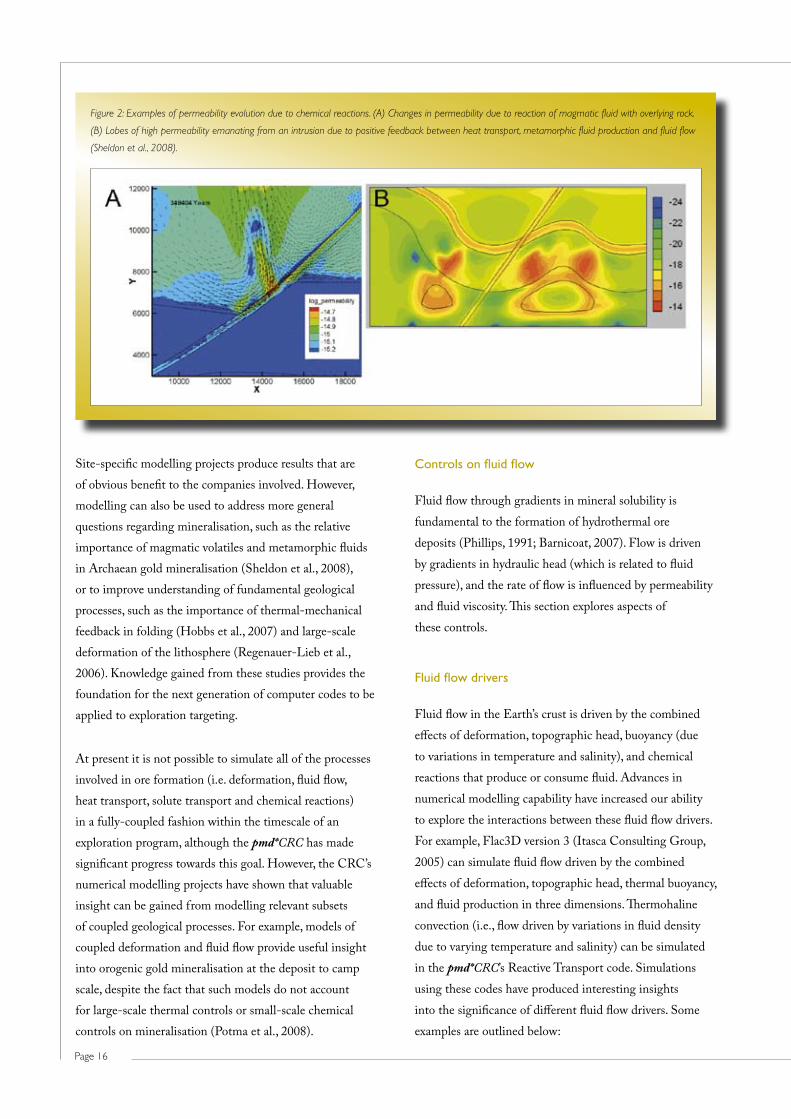
granodiorite body at Tarmoola, WA (Potma et al., 2007) (Figure 1B) have demonstrated the potential for generating precise targets from models based on realistic geometries. Further examples involving curved and intersecting faults are in Appendix 1. Another strength of numerical modelling is the ability to explore complex effects arising from feedback between coupled geological processes, e.g. channelling of fluid flow due to reaction-permeability feedback (Figure 2). Numerical modelling also enables us to quantify the dimension of time, providing answers to such questions as: How long does it take to produce an economic deposit by the proposed mechanism? What is the time interval between events in the conceptual model? For example, numerical models of regional metamorphic fluid production revealed that the fluid is produced and escapes from the crust within ~1 to 10 million years (Sheldon et al., 2008).
Another valuable aspect of numerical modelling is the ability to test the sensitivity of the system to variations in geometry (e.g. fault strike and dip), deformation regime (e.g. varying the direction of shortening) or properties (e.g. rock strength, permeability). Tools developed by the pmd*CRC enable researchers to define, run and analyse multiple versions of the same model with ease. This approach can be used for reverse-engineering of a known deposit (adjusting the model until it reproduces known features), or as a predictive tool, e.g. identifying optimum fault orientations and intersection angles for mineralisation. The value of this approach was illustrated by the Kundana modelling project, which resulted in two high-grade gold intercepts being drilled (Potma et al., 2008).
This document summarises some of the advances in understanding achieved through the development and application of numerical modelling technologies, using examples from terrane and one-on-one projects and material from the modelling (M9) and fluids (F6) projects. Technical details can be found in other sections of this report.
Benefits of numerical modelling
Much of this report focuses on advances in numerical modelling capability. There has been an equally important advance in our understanding of its benefits and the role it can play in mineral exploration.
The first stage in a numerical modelling project is to define conceptual models (hypotheses) describing the processes that resulted in mineralisation. This process forces one to be specific about the system’s geometry and properties, and the processes that occurred within it. Some argue that the results of numerical models are obvious once the conceptual model has been defined. This may be true of simple models (e.g. a model containing a single, straight fault), but is not when the model has a degree of geometrical complexity and/or coupling between geological processes. For example, a model of deformation and fluid flow around an intrusive body with a realistic geometry can reveal the exact location(s) of maximum dilation, shear strain and fluid focusing relative to the intrusion, whereas a simplified representation of the intrusion (e.g. an ellipsoid) will not. Numerical models of deformation and fluid flow around basalt domes in western Victoria (Rawling et al., 2006; Schaubs et al., 2006) (Figure 1A) and a
Figure 1: Examples of targets generated
from numerical models of deformation
and fluid flow with realistic geometries.
(A) Targets (green dots) at southern end
of the Kewell basalt dome (yellow surface)
in western Victoria based on coincident
anomalies of dilation (red surface), fluid
flux (arrows), and gold anomaly in air-core
geochemistry. Pink surface = present-day
erosion level. (B) Coincident anomalies of
shear strain, integrated fluid flux and dilation
represent three targets around the Tarmoola
granodiorite body (pink surface), WA. Orange
surface = Tarmoola pit.
Page 16
Controls on fluid flow
Fluid flow through gradients in mineral solubility is fundamental to the formation of hydrothermal ore deposits (Phillips, 1991; Barnicoat, 2007). Flow is driven by gradients in hydraulic head (which is related to fluid pressure), and the rate of flow is influenced by permeability and fluid viscosity. This section explores aspects of these controls.
Fluid flow drivers
Fluid flow in the Earth’s crust is driven by the combined effects of deformation, topographic head, buoyancy (due to variations in temperature and salinity), and chemical reactions that produce or consume fluid. Advances in numerical modelling capability have increased our ability to explore the interactions between these fluid flow drivers. For example, Flac3D version 3 (Itasca Consulting Group, 2005) can simulate fluid flow driven by the combined effects of deformation, topographic head, thermal buoyancy, and fluid production in three dimensions. Thermohaline convection (i.e., flow driven by variations in fluid density due to varying temperature and salinity) can be simulated in the pmd*CRC’s Reactive Transport code. Simulations using these codes have produced interesting insights into the significance of different fluid flow drivers. Some examples are outlined below:
Site-specific modelling projects produce results that are of obvious benefit to the companies involved. However, modelling can also be used to address more general questions regarding mineralisation, such as the relative importance of magmatic volatiles and metamorphic fluids in Archaean gold mineralisation (Sheldon et al., 2008), or to improve understanding of fundamental geological processes, such as the importance of thermal-mechanical feedback in folding (Hobbs et al., 2007) and large-scale deformation of the lithosphere (Regenauer-Lieb et al., 2006). Knowledge gained from these studies provides the foundation for the next generation of computer codes to be applied to exploration targeting.
At present it is not possible to simulate all of the processes involved in ore formation (i.e. deformation, fluid flow, heat transport, solute transport and chemical reactions) in a fully-coupled fashion within the timescale of an exploration program, although the pmd*CRC has made significant progress towards this goal. However, the CRC’s numerical modelling projects have shown that valuable insight can be gained from modelling relevant subsets of coupled geological processes. For example, models of coupled deformation and fluid flow provide useful insight into orogenic gold mineralisation at the deposit to camp scale, despite the fact that such models do not account for large-scale thermal controls or small-scale chemical controls on mineralisation (Potma et al., 2008).
Figure 2: Examples of permeability evolution due to chemical reactions. (A) Changes in permeability due to reaction of magmatic fluid with overlying rock.
(B) Lobes of high permeability emanating from an intrusion due to positive feedback between heat transport, metamorphic fluid production and fluid flow
(Sheldon et al., 2008).

Page 17
pmd*CRC ProjeCtS M4, M9 and F6 Final rePort
Models of thermohaline convection reveal interesting flow patterns (Figure 3.) resulting from the different transport rates of heat (which diffuses through the solid and fluid) and salt (which remains in the fluid phase). This capability has not yet been applied to an exploration scenario but will be useful for modelling magmatic systems, which are characterised by large gradients in temperature and salinity.
Fluid flow boundary conditions
Fluid flow regimes in numerical models are influenced not only by the processes and fluid drivers that are represented within the model, but also by the boundary conditions that are applied to the edges of the model. Boundary conditions represent interaction of the model with its surroundings. Possible boundary conditions for fluid flow are a specified fluid flux (i.e. fluid moving in to or out of the model at a constant rate; zero flux represents an impermeable boundary) or specified fluid pressure (allowing fluid to move across the boundary at a variable rate).
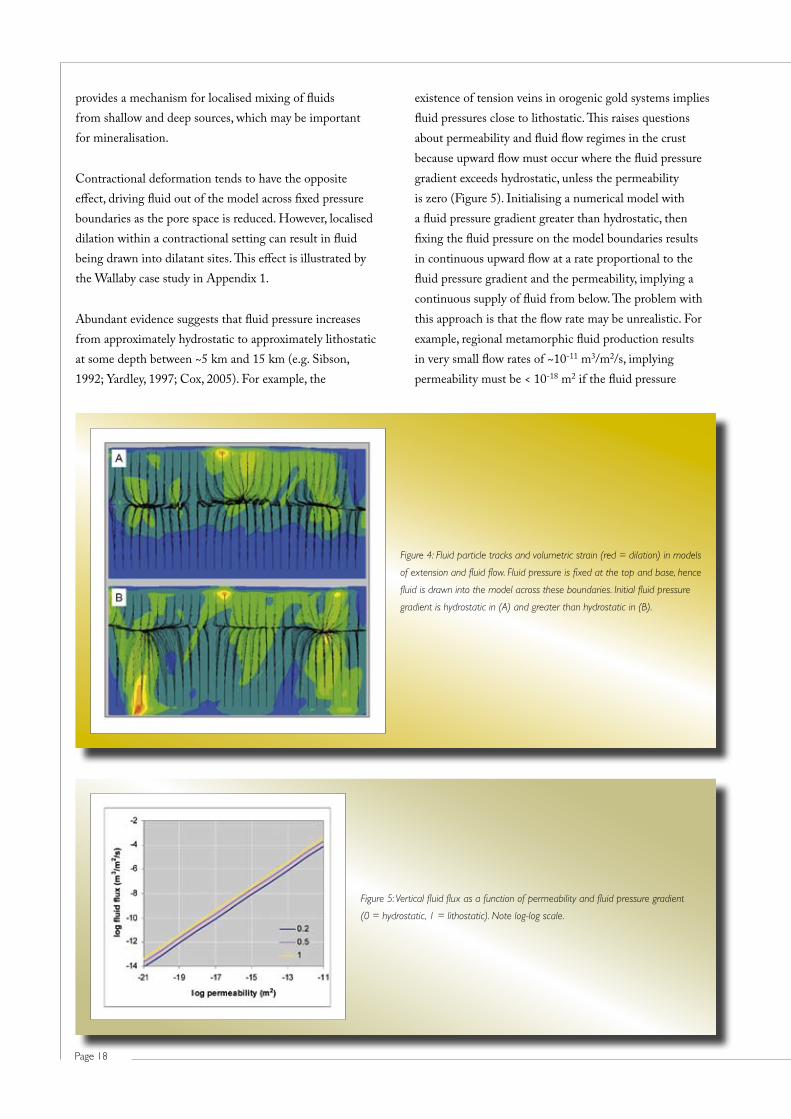
Extensional deformation results in fluid being drawn into a model across fixed pressure boundaries, to counteract the reduction in fluid pressure within the model due to expansion of the pore space. Thus, if fluid pressure is fixed along the top boundary of a model (e.g. representing the Earth’s surface) and all other boundaries are impermeable, extensional deformation results in downward flow from the surface. This could represent downflow of sea water, meteoric water or basinal brine. If fluid pressure is fixed at the base of the model as well as the top, fluid will move up from the base and down from the top, meeting at a depth determined by the strain rate, permeability distribution and the fluid pressure gradient between the model’s top and base. Fluid tends to migrate towards dilatant sites at this depth (Figure 4). Extensional deformation therefore
Oliver et al. (2006) used FLAC to explore flow regimes across a faulted basement-cover interface. Their model showed extensional deformation at a moderate strain rate could override thermal convection, with convection resuming shortly after deformation had ended. The same effect was observed in a three-dimensional version of the model, providing insight into the shape and location of the convection cells relative to the basement-cover interface (see Appendix 1 for more details). The outcomes of this work have implications for the formation of Mt Isa-style Pb-Zn ores and other extension-related basinal deposits.
Section 2.9 of this report describes the development of algorithms for simulating metamorphic and magmatic fluid production in Flac3D, where the rate of fluid production is determined by the rate of heating or cooling. Sheldon et al. (2008) used this methodology in a model representing regional metamorphism in the Yilgarn, which showed the rate of fluid flow due to regional metamorphic fluid production is very small unless the fluid is focused into permeable fault zones. It was found that metamorphic fluid is produced and passes through the crust in less than 10 million years, unless it is trapped in dilatant sites. Thus, the timing of metamorphic fluid production relative to tectonic events is important in determining the fate of the metamorphic fluid and its potential to be involved in mineralisation. Other models showed that release of magmatic volatiles from shallow-level intrusions, and accompanying metamorphic fluid release in the surrounding rocks, can result in rotation of the principal stress axes and consequent effects on the orientation of fluid flow pathways around intrusions. This could explain radial patterns of veins and dykes around some intrusions, e.g. the Jupiter syenite in the Eastern Yilgarn (Duuring et al., 2000).
Figure 3: Patterns of salinity, fluid flow vectors, fluid density and temperature due to thermohaline convection. Model is initialised with an internal box of
higher salinity, lower temperature fluid. See Section 2.4 for details.
Page 18
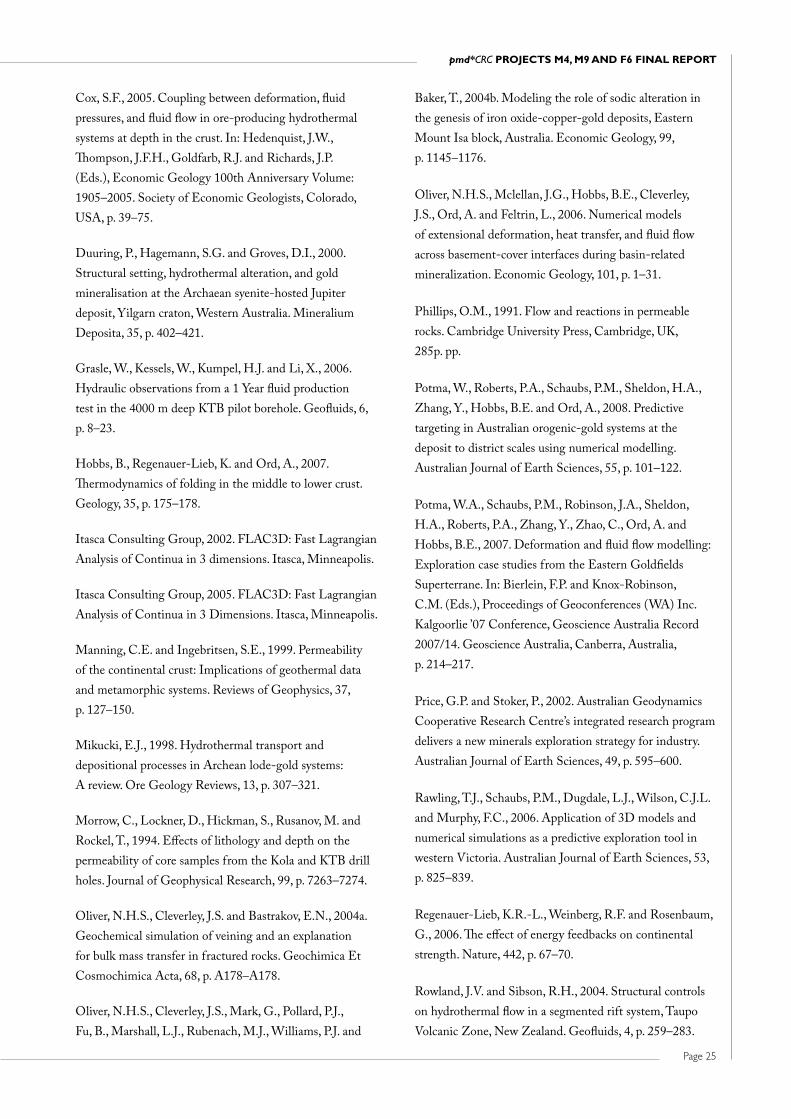
existence of tension veins in orogenic gold systems implies fluid pressures close to lithostatic. This raises questions about permeability and fluid flow regimes in the crust because upward flow must occur where the fluid pressure gradient exceeds hydrostatic, unless the permeability is zero (Figure 5). Initialising a numerical model with a fluid pressure gradient greater than hydrostatic, then fixing the fluid pressure on the model boundaries results in continuous upward flow at a rate proportional to the fluid pressure gradient and the permeability, implying a continuous supply of fluid from below. The problem with this approach is that the flow rate may be unrealistic. For example, regional metamorphic fluid production results in very small flow rates of ~10-11 m3/m2/s, implying permeability must be < 10-18 m2 if the fluid pressure
provides a mechanism for localised mixing of fluids from shallow and deep sources, which may be important for mineralisation.
Contractional deformation tends to have the opposite effect, driving fluid out of the model across fixed pressure boundaries as the pore space is reduced. However, localised dilation within a contractional setting can result in fluid being drawn into dilatant sites. This effect is illustrated by the Wallaby case study in Appendix 1.
Abundant evidence suggests that fluid pressure increases from approximately hydrostatic to approximately lithostatic at some depth between ~5 km and 15 km (e.g. Sibson, 1992; Yardley, 1997; Cox, 2005). For example, the
Figure 5: Vertical fluid flux as a function of permeability and fluid pressure gradient
(0 = hydrostatic, 1 = lithostatic). Note log-log scale.
Figure 4: Fluid particle tracks and volumetric strain (red = dilation) in models
of extension and fluid flow. Fluid pressure is fixed at the top and base, hence
fluid is drawn into the model across these boundaries. Initial fluid pressure
gradient is hydrostatic in (A) and greater than hydrostatic in (B).

Page 19
pmd*CRC ProjeCtS M4, M9 and F6 Final rePort
the case in which constant fluid properties are assumed (Straus and Schubert, 1977).
Varying fluid properties are routinely considered in reactive transport simulations (e.g. an equation of state for pure water has been incorporated into the Reactive Transport utility developed by the pmd*CRC), but less commonly in models of coupled deformation and fluid flow. pmd*CRC researchers have addressed this deficiency by writing functions to represent variation in fluid viscosity with temperature in Flac3D and by developing an algorithm to invoke the equation-of-state module of the RT utility from a Flac3D simulation (see section 2.9).
Permeability
Estimates of the permeabilities of upper crustal rocks span 14 orders of magnitude, ranging from ~10-9 m2 for karst limestone to 10-23 m2 for unfractured crystalline rocks (see compilations in Clauser (1992) and Rowland and Sibson (2004)). Permeability is a key factor in determining the rate of fluid flow. It also controls the direction of flow if there are spatial variations in permeability. For example, flow will become focused into a fault zone if the fault is more permeable than the surrounding rocks (Phillips, 1991). This is important for hydrothermal mineralisation; for example, the fluid flux due to regional metamorphism is about 1000 times too small to account for gold mineralisation, unless it is focused into a narrow fault zone (Cox, 1999; Sheldon et al., 2008). The relative rates of advection, diffusion/dispersion and chemical reactions determine the location of mineralisation relative to the fault (Zhao et al., 2007).
On the laboratory scale, permeability varies with pressure, temperature and stress regime (e.g. Morrow et al., 1994; Zharikov et al., 2003). These small-scale measurements do not account for the effect of fractures, which dominate permeability on scales greater than a few metres (Clauser, 1992). Estimates of permeability on a larger scale can be obtained from borehole pumping tests (e.g. Grasle et al., 2006), empirical relationships between fracture spacing, aperture and permeability (e.g. Phillips, 1991), the progress of metamorphic reactions and heat fluxes in geothermal systems (Manning and Ingebritsen, 1999), and numerical models of fluid flow in fracture networks (e.g. Caine and Forster, 1999).
gradient is lithostatic (Figure 5). There is no reason to assume that an upward flux occurs everywhere at all times. How, then, can supralithostatic fluid pressures be maintained? Some argue the crust is essentially dry except where fluid is being produced, for example by metamorphic reactions (Yardley, 1997; Yardley and Valley, 1997). Time-dependent (viscous) compaction may also play a role in maintaining high fluid pressures. Models of viscous compaction and corresponding permeability evolution predict the development of a hydrostatic-lithostatic fluid pressure interface at some depth in the crust, and migrating “waves” of fluid (Connolly, 1997; Sheldon and Wheeler, 2003). In the absence of this deformation mechanism it is impossible to maintain fluid overpressure without a continuous supply of fluid. Incorporating such behaviour into numerical models applied to mineral exploration is a challenge for the future.
Most deformation-fluid flow modelling by pmd*CRC researchers has used an elastic-plastic constitutive model, hence these models cannot generate or maintain a supra-lithostatic fluid pressure gradient unless there is a continuous supply of fluid into the base of the model. Unrealistic fluid fluxes can be avoided in such models by specifying a fluid flux boundary condition rather than fixed fluid pressure and assigning suitably low permeabilities to parts of the model that represent overpressured regions of the crust. Alternatively, metamorphic fluid production can be modelled by imposing fluid production as a function of temperature change (see section 2.9). For models that represent a region within the overpressured part of the crust, fluid overpressure without anomalous fluid fluxes can be achieved by initialising the fluid pressure with a hydrostatic gradient but suprahydrostatic fluid pressure, then either fixing the pressure at the top and/or base, or leaving boundaries impermeable.
Fluid properties
Natural pore fluids have properties (e.g. viscosity, specific heat capacity, density) that vary in a highly non-linear fashion with pressure, temperature and composition. These non-linear variations in fluid properties have a profound effect on fluid flow regimes; for example, the minimum permeability for the onset of free thermal convection is reduced by between one and two orders of magnitude if varying fluid properties are taken into account, relative to

Page 20
(e.g. Bruhn et al., 1994; Barton et al., 1995). This implies faults have a higher time-integrated permeability than the surrounding rock. It is common to assign a uniform, high permeability to fault zones in numerical models. However, field studies indicate permeability may be highly variable along faults, with jogs and bends favourable sites for fluid flow and mineralisation. It is often the minor faults and fractures at these sites that host mineralisation, rather than the main fault. This can be explained by an increase in “damage rate” around fault jogs and bends after a slip event on the main fault, while the fault itself enters a healing regime and becomes less permeable (Sheldon and Micklethwaite, 2007; Figure 7).
Faults in high-porosity rocks may behave differently, due to variation in the deformation mechanism with porosity and confining pressure. Faults in high-porosity siliciclastic rocks are likely to be less permeable than the undeformed rock at depths shallower than ~3–4 km (Sheldon et al.,
Many authors have noted a tendency for permeability to decrease with increasing depth in the crust. Figure 6 shows two permeability-depth curves representing “average” crustal permeability, based on small-scale laboratory measurements (Shmonov et al., 2003) and field estimates (Manning and Ingebritsen, 1999). The difference between the curves is consistent with scale-dependence of permeability. While the meaning of “average” in the context of crustal permeability is questionable, these curves provide useful insight into typical permeability values and the consequences for fluid flow. In particular, it can be shown that permeabilities must be at least an order of magnitude greater than the upper limit of these curves to permit free thermal convection (see section 2.10 for details). Such high values may be attained in faults or in porous sedimentary rocks unless thin, low permeability layers are present.
Abundant evidence suggests faults act as preferential fluid pathways, at least while they are tectonically active
Figure 6: “Average” permeability of the crust as a function of depth, based on
laboratory measurements (Shmonov et al., 2003) and field estimates (Manning
and Ingebritsen, 1999).
Figure 7: Model of damage rate (representing permeability
enhancement) around an idealised strike-slip fault.
(A) Geometry. Red area indicates fault. (B) Contours and
isosurface of damage rate. Damage is enhanced around the
fault tip line and in lobes extending from the ends of the
fault, but not within the fault itself.

Page 21
pmd*CRC ProjeCtS M4, M9 and F6 Final rePort
which fluid of a constant composition is fed into the left of the models, reacts with rock in the first reactor and then is displaced to the right by the next aliquot of fluid. The reacted fluid then reacts with the next “compartment” of rock, is displaced, and so on. This approach is the closest possible approximation to reactive transport that can be achieved in HCh. It does not explicitly take account of time, distance, reaction kinetics or fluid flow pathways. The results are illustrated in Figure 8.
Note the contrast between the models due to the differing proportions of H2S/SO4 and CH4/CO2. In a strongly reduced fluid (Figure 8a), interaction with Fe-oxide + Fe-silicate bearing rocks produces pyrrhotite zones in conjunction with the commonly observed silica-carbonate-white mica alteration, favouring broad gold deposition across the sulphidation zone. However, when the H2S/SO4 ratio is decreased, initial sulphidation of the wallrocks makes way for a narrow anhydrite zone (Figure 8b), and when the fluid sulphur is exhausted, the relatively low CH4/CO2 ratio results in oxidation of the host metabasalt. Thus, a change from reduced to oxidised mineral assemblages in time and space may not reflect the operation of two separate fluids, nor even a temperature gradient. Rather, it may reflect a balance between differing buffers during progressive infiltration of a single fluid. Fluid mixing, infiltration and rock buffering of fluid all provide scenarios in which steep geochemical gradients can lead to gold precipitation.
Reactive transport modelling: Fluid-rock reaction and reaction potential
Alteration and mineralisation require a chemically-reactive fluid to be transported from its source to the site of deposition/alteration without losing its reactivity. Sometimes the inferred source is kilometres away from the site of deposition. 1D reaction path models, such as those performed using HCh (see example above), tell us nothing about the distances and timescales over which fluids can maintain their reactivity. Reactive transport modelling introducestimeanddistanceandillustratesthedifficultyintransporting reactive fluid from source to deposition site. An example of this problem is illustrated by unconformity-related uranium systems. A conceptual model proposes that uranium is scavenged from sandstone by infiltrating basinal brine before being transported to the basement where it is
2006). Hence, faults in porous sedimentary rocks may act as barriers to flow rather than fluid conduits. This has implications for sediment-hosted mineralisation.
Given the huge range of permeabilities in the Earth’s crust, and the number of factors influencing permeability, it can be hard to decide what values should be used in numerical models. A pragmatic approach is to use laboratory measurements as a guide to permeability contrasts between rock types within the model but to increase the permeability by an order of magnitude relative to the laboratory-measured values to account for scale dependence. Permeability may then be modified during a model run to reflect the effects of deformation or chemical reactions. For example, pmd*CRC researchers have developed algorithms representing permeability increase with shear or tensile failure to use in deformation-fluid flow simulations, while permeability increase/decrease due to mineral dissolution/precipitation is incorporated in reactive transport models. The latter have shown interesting feedback effects, such as displacement of a convective upwelling as the fluid pathway becomes blocked by precipitation of quartz cement (Cleverley, 2008).
Fluid chemistry and solute transport
Geochemical modelling with HCh (Shvarov and Bastrakov, 1999) has been used and developed throughout the pmd*CRC. Several publications from the fluids program team illustrate the learnings from HCh modelling of mineral systems (Cleverley et al., 2004a; Cleverley et al., 2004b; Oliver et al., 2004a; Oliver et al., 2004b; Cleverley and Oliver, 2005). The progression from geochemical modelling to reactive transport modelling in the CRC’s second half allowed many more phenomena to be explored, involving chemical reactions coupled with heat and mass transport (Cleverley et al., 2006a; Cleverley et al., 2006b; Cleverley, 2007, 2008). This section illustrates some of the key understandings that have resulted from the use of geochemical and reactive transport modelling.
Geochemical modelling: Sulphidation and redox in gold systems
One possible mechanism for precipitation of gold in greenstone systems is the destabilisation of soluble gold sulphur species (e.g. gold bisulphide) on precipitation of sulphides (e.g. Mikucki, 1998). Sulphidation has been modelled using a reactor-style infiltration algorithm in

Page 22
Figure 9 compares reactive transport models of a simple unconformity uranium scenario (Schaubs and Fisher, 2008), in which two basin units sit above an unconformity with underlying basement cut by a permeable fault. The models show the distribution of uraninite after the infiltration of oxidised basinal brine into the basement, driven by the high
precipitated. The fundamental control on deposition is the redox gradient between the basin (oxidised) and basement (reduced). Reactive transport models of this scenario (SchaubsandFisher,2008)showitisextremelydifficulttotransport oxidised fluid through typical sedimentary rocks without it losing its capacity to transport uranium.
Figure 9: Uraninite
distribution in two reactive
transport models of
oxidised basinal brine
interacting with U-rich
sandstone. The sandstone
contains chlorite in A but
is clean in B, which affects
the redox capacity of
the infiltrating fluid. Scale
marked in metres.
Figure 8: HCh model results for infiltration of
fluid (from left to right) with NaCl molality 0.2,
KCl 0.5, CaCl2 0.4, FeCl2 0.03, H4SiO4 0.035
(and other redox and sulphur parameters
as below) into metabasalt with mineralogy
shown on the right of the diagrams (buffering
log aO2 –31). The models were run under
isothermal, isobaric conditions at 380°C and
250 MPa. The x-axis is the nominal distance
the front has travelled for a fixed time and
fluid velocity. Alternately it can be regarded as
the time taken for a reaction front to reach
a certain distance for a given fluid flow rate.
The last step shown on the log aO2 diagrams
represents the limit of infiltration of the exotic
fluid. A) Reduced fluid with molality of CO2
2.0, CH4 0.1, H2S 0.1 and SO2 10-10, pH of
3.5 and log aO2 –32.0 showing sulphidation
assemblages characteristic of proximal zones
of many ore deposits; B) Moderately reduced
fluid with CO2 molality 4.0, CH4 0.01, H2S 0.1
and SO2 10-7, pH of 3.25 and log aO2 –31.1,
in which exhaustion of the fluid’s sulphidation
capacity leads to formation of oxidised
assemblages ahead of the front, including the
anhydrite- and hematite-bearing assemblages
found in several large deposits in the Yilgarn.

Page 23
pmd*CRC ProjeCtS M4, M9 and F6 Final rePort
Fracturing and brecciation are critical in the formation of ore deposits but are hard to model realistically using continuum codes. Particle codes offer an alternative, which is better suited to problems involving large strains and the creation of fractures and voids. Section 2.11 describes recent advances in the application of particle codes to geological problems. Of particular interest is the use of particle codes to simulate fluid-driven deformation, such as melt intrusion and the formation of hydrothermal breccias.
Damage mechanics is another approach that is useful for modelling deformation in the brittle regime. This technique has yielded insight into the distribution of permeability and ore deposits relative to major faults (see section 2.8). The advantage of damage mechanics over conventional constitutive models, such as Mohr Coulomb, is that it accounts for irreversible deformation before macroscopic failure. Furthermore, the concept of damage is readily associated with permeability and can be used to explore the consequences of deformation for fluid flow. Damage mechanics can be included in a thermodynamic framework for rock deformation, through consideration of the energy associated with formation and healing of microcracks. A thermodynamic approach that combines damage mechanics with temperature-dependent visco-elastic behaviour could be used to simulate the entire thickness of the lithosphere, predicting the transition from brittle to ductile behaviour in a self-consistent manner.
Conclusion
This document illustrates the value gained from the development and application of numerical modelling techniques during the pmd*CRC. These techniques have improved our understanding of mineral systems and how to model them. New software and tools developed within the CRC’s Enabling Technologies program have expanded the range of scenarios that can be modelled. Experience gained from the application of these tools to industry problems has produced many useful insights into mineralisation processes. In addition, pmd*CRC researchers have made significant progress in developing the next generation of modelling tools to enable simulation of processes beyond the scope of the current tool kit.
References
Barnicoat, A.C., 2007. Putting it all together: Anatomy of a giant mineral system. In: Bierlein, F.P. and Knox-Robinson,
density of the brine relative to the basement pore fluid. The sandstone in Figure 9a contains chlorite, whereas that in Figure 9b does not. This simple mineralogical control on the rock’s reduction capacity has a strong influence on the ability to maintain the redox state of the fluids to allow uraninite dissolution, transport and precipitation in the basement (compare Figures 9a and 9b).
The need for fluid to access a permeable pathway and travel between two locations while maintaining its strong chemical reactivity is common to many mineral systems. Future developments of the reactive transport code will include reaction kinetics, which may provide the key to understanding how metal can be transported over long distances.
Techniques for the future
pmd*CRC researchers have begun developing new approaches for modelling crustal processes to address the limitations of current methods. These developments will be included in the modelling tools of the future.
Section 2.15 describes a thermodynamically consistent approach to modelling ore formation in the Earth’s crust, based around the concepts of non-equilibrium thermodynamics and maximum entropy production. Hobbs et al. (2007) postulated that giant ore bodies form when coupled, non-equilibrium processes interact to maximise the rate of entropy production in the system. This occurs when thermo-mechanical and chemical feedbacks drive localised permeability enhancement, tapping into sources of heat and ore-forming fluids in the lower crust and upper mantle. Computer simulations incorporating thermo-mechanical feedback predict a variety of geological features not readily produced using conventional modelling techniques. Examples include folding, boudinage, listric faults, low-angle detachments and metamorphic core complexes. These features are important on the 100 m to 1000 m scale. Adding chemical reaction-diffusion processes into the formulation creates deformation features on the micron to centimetre scale. Simulations involving strong coupling between thermal, chemical and mechanical processes can predict a wider range of geological phenomena than is possible with the techniques that are currently applied to mineral exploration. In particular, this coupling opens the possibility of modelling processes in the deep (ductile) parts of the Earth’s crust and upper mantle.

Page 24
exploration. Abstracts for the June 2008 pmd*CRC conference, Geoscience Australia Record 2008/09. Geoscience Australia, Canberra, Australia, p. 29–37.
Cleverley, J.S. and Bastrakov, E.N., 2005. K2GWB: Utility for generating thermodynamic data files for The Geochemist’s Workbench (R) at 0–1000 degrees C and 1–5000 bar from UT2K and the UNITHERM database. Computers & Geosciences, 31, p. 756–767.
Cleverley, J.S., Hornby, P. and Poulet, T., 2006a. Pmd*RT: combined fluid, heat and chemical modellling and its application to Yilgarn geology. In: Barnicoat, A.C. and Korsch, R.J. (Eds.), Predictive Mineral Discovery at the Sharp End 2006/07. Geoscience Australia, p. 23–28.
Cleverley, J.S., Hornby, P. and Poulet, T., 2006b. Reactive transport modelling in hydrothermal systems using the Gibbs minimisation approach. Geochimica Et Cosmochimica Acta, 70, p. A106–A106.
Cleverley, J.S. and Oliver, N.H.S., 2005. Comparing closed system, flow-through and fluid infiltration geochemical modelling: examples from K-alteration in the Ernest Henry Fe-oxide-Cu-Au system. Geofluids, 5, p. 289–307.
Cleverley, J.S., Oliver, N.H.S. and Bastrakov, E.N., 2004a. Reactor style modelling of fluid-rock infilatration and interaction using the HCh software package. Geochimica Et Cosmochimica Acta, 68, p. A187–A187.
Cleverley, J.S., Oliver, N.H.S., Bastrakov, E.Y. and Shvarov, Y.Y., 2004b. Geochemical modelling tools in predictive mineral discovery. In: Muhling, J. (Ed.), SEG 2004 Predictive Mineral Discovery Under Cover. Society of Economic Geologists, Perth.
Connolly, J.A.D., 1997. Devolatilization-Generated Fluid Pressure and Deformation-Propagated Fluid Flow During Prograde Regional Metamorphism. Journal of Geophysical Research, 102, p. 18149–18173.
Cox, S.F., 1999. Deformational controls on the dynamics of fluid flow in mesothermal gold systems. In: McCaffrey, K.J.W., Lonergan, L. and Wilkinson, J.J. (Eds.), Fractures, fluid flow and mineralization. Geological Society of London Special Publications 155. Geological Society of London, London, UK, p. 123–140.
C.M. (Eds.), Proceedings of Geoconferences (WA) Inc. Kalgoorlie ’07 Conference, Geoscience Australia Record 2007/14. Geoscience Australia, Canberra, Australia, p. 47–51.
Barnicoat, A.C., 2008. The pmd*CRC’s mineral systems approach. In: Korsch, R.J. and Barnicoat, A.C. (Eds.), New Perspectives: The foundations and future of Australian exploration. Abstracts for the June 2008 pmd*CRC conference, Geoscience Australia Record 2008/09. Geoscience Australia, Canberra, Australia, p. 1–6.
Barton, C.A., Zoback, M.D. and Moos, D., 1995. Fluid-Flow Along Potentially Active Faults in Crystalline Rock. Geology, 23, p. 683–686.
Bastrakov, E., Shvarov, Y., Girvan, S., Cleverley, J., McPhail, D. and Wyborn, L.A.I., 2005. FreeGs: A web-enabled thermodynamic database for geochemical modelling. Geochimica Et Cosmochimica Acta, 69, p. A845–A845.
Bethke, C.M., 1996. Geochemical Reaction Path Modeling: Concepts and applications. Oxford University Press, New York, 397 pp.
Bruhn, R.L., Parry, W.T., Yonkee, W.A. and Thompson, T., 1994. Fracturing and hydrothermal alteration in normal-fault zones. Pure and Applied Geophysics, 142, p. 609–644.
Caine, J.S. and Forster, C.B., 1999. Fault zone architecture and fluid flow: Insights from field data and numerical modeling. In: Haneberg, W.C., Mozley, P.S., Moore, J.C. and Goodwin, L.B. (Eds.), Faults and subsurface fluid flow in the shallow crust. Geophysical Monographs 113. AGU, Washington DC, p. 101–127.
Clauser, C., 1992. Permeability of crystalline rocks. EOS, 73, p. 231–237.
Cleverley, J.S., 2007. Large scale finite element reactive transport modelling as a tool to aid understanding and prediction in mineral systems, SGA2007. Society for Geology Applied to Mineral Deposits, Dublin.
Cleverley, J.S., 2008. Deposition: Reactive transport modelling. In: Korsch, R.J. and Barnicoat, A.C. (Eds.), New Perspectives: The foundations and future of Australian
Page 25
pmd*CRC ProjeCtS M4, M9 and F6 Final rePort
Baker, T., 2004b. Modeling the role of sodic alteration in the genesis of iron oxide-copper-gold deposits, Eastern Mount Isa block, Australia. Economic Geology, 99, p. 1145–1176.
Oliver, N.H.S., Mclellan, J.G., Hobbs, B.E., Cleverley, J.S., Ord, A. and Feltrin, L., 2006. Numerical models of extensional deformation, heat transfer, and fluid flow across basement-cover interfaces during basin-related mineralization. Economic Geology, 101, p. 1–31.
Phillips, O.M., 1991. Flow and reactions in permeable rocks. Cambridge University Press, Cambridge, UK, 285p. pp.
Potma, W., Roberts, P.A., Schaubs, P.M., Sheldon, H.A., Zhang, Y., Hobbs, B.E. and Ord, A., 2008. Predictive targeting in Australian orogenic-gold systems at the deposit to district scales using numerical modelling. Australian Journal of Earth Sciences, 55, p. 101–122.
Potma, W.A., Schaubs, P.M., Robinson, J.A., Sheldon, H.A., Roberts, P.A., Zhang, Y., Zhao, C., Ord, A. and Hobbs, B.E., 2007. Deformation and fluid flow modelling: Exploration case studies from the Eastern Goldfields Superterrane. In: Bierlein, F.P. and Knox-Robinson, C.M. (Eds.), Proceedings of Geoconferences (WA) Inc. Kalgoorlie ’07 Conference, Geoscience Australia Record 2007/14. Geoscience Australia, Canberra, Australia, p. 214–217.
Price, G.P. and Stoker, P., 2002. Australian Geodynamics Cooperative Research Centre’s integrated research program delivers a new minerals exploration strategy for industry. Australian Journal of Earth Sciences, 49, p. 595–600.
Rawling, T.J., Schaubs, P.M., Dugdale, L.J., Wilson, C.J.L. and Murphy, F.C., 2006. Application of 3D models and numerical simulations as a predictive exploration tool in western Victoria. Australian Journal of Earth Sciences, 53, p. 825–839.
Regenauer-Lieb, K.R.-L., Weinberg, R.F. and Rosenbaum, G., 2006. The effect of energy feedbacks on continental strength. Nature, 442, p. 67–70.
Rowland, J.V. and Sibson, R.H., 2004. Structural controls on hydrothermal flow in a segmented rift system, Taupo Volcanic Zone, New Zealand. Geofluids, 4, p. 259–283.
Cox, S.F., 2005. Coupling between deformation, fluid pressures, and fluid flow in ore-producing hydrothermal systems at depth in the crust. In: Hedenquist, J.W., Thompson, J.F.H., Goldfarb, R.J. and Richards, J.P. (Eds.), Economic Geology 100th Anniversary Volume: 1905–2005. Society of Economic Geologists, Colorado, USA, p. 39–75.
Duuring, P., Hagemann, S.G. and Groves, D.I., 2000. Structural setting, hydrothermal alteration, and gold mineralisation at the Archaean syenite-hosted Jupiter deposit, Yilgarn craton, Western Australia. Mineralium Deposita, 35, p. 402–421.
Grasle, W., Kessels, W., Kumpel, H.J. and Li, X., 2006. Hydraulic observations from a 1 Year fluid production test in the 4000 m deep KTB pilot borehole. Geofluids, 6, p. 8–23.
Hobbs, B., Regenauer-Lieb, K. and Ord, A., 2007. Thermodynamics of folding in the middle to lower crust. Geology, 35, p. 175–178.
Itasca Consulting Group, 2002. FLAC3D: Fast Lagrangian Analysis of Continua in 3 dimensions. Itasca, Minneapolis.
Itasca Consulting Group, 2005. FLAC3D: Fast Lagrangian Analysis of Continua in 3 Dimensions. Itasca, Minneapolis.
Manning, C.E. and Ingebritsen, S.E., 1999. Permeability of the continental crust: Implications of geothermal data and metamorphic systems. Reviews of Geophysics, 37, p. 127–150.
Mikucki, E.J., 1998. Hydrothermal transport and depositional processes in Archean lode-gold systems: A review. Ore Geology Reviews, 13, p. 307–321.
Morrow, C., Lockner, D., Hickman, S., Rusanov, M. and Rockel, T., 1994. Effects of lithology and depth on the permeability of core samples from the Kola and KTB drill holes. Journal of Geophysical Research, 99, p. 7263–7274.
Oliver, N.H.S., Cleverley, J.S. and Bastrakov, E.N., 2004a. Geochemical simulation of veining and an explanation for bulk mass transfer in fractured rocks. Geochimica Et Cosmochimica Acta, 68, p. A178–A178.
Oliver, N.H.S., Cleverley, J.S., Mark, G., Pollard, P.J., Fu, B., Marshall, L.J., Rubenach, M.J., Williams, P.J. and
Page 26
pmd*CRC ProjeCtS M4, M9 and F6 Final rePort
and pressure-dependent thermodynamic and transport properties. Journal of Geophysical Research, 82, p. 325–333.
Wyborn, L.A.I., Heinrich, C.A. and Jaques, A.L., 1994. Australian Proterozoic mineral systems: Essential ingredients and mappable criteria. In: Hallenstein, C.P. (Ed.) Australian mining looks North; the challenges and choices. 1994 AusIMM annual conference, Australian Institute of Mining and Metallurgy Publication Series 5/94. Australasian Institute of Mining and Metallurgy, p. 109–115.
Yardley, B.W.D., 1997. The evolution of fluids through the metamorphic cycle. In: Jamtveit, B. and Yardley, B.W.D. (Eds.), Fluid flow and transport in rocks. Chapman and Hall, London, p. 99–122.
Yardley, B.W.D. and Valley, J.W., 1997. The Petrologic Case for a Dry Lower Crust. Journal of Geophysical Research, 102, p. 12173–12185.
Zhao, C., Hobbs, B.E., Ord, A., Hornby, P., Peng, S. and Liu, L., 2007. Mineral precipitation associated with vertical fault zones: the interaction of solute advection, diffusion and chemical kinetics. Geofluids, 7, p. 3–18.
Zharikov, A.V., Vitovtova, V.M., Shmonov, V.M. and Grafchikov, A.A., 2003. Permeability of the rocks from the Kola superdeep norehole at high temperature and pressure: Implication to fluid dynamics in the continental crust. Tectonophysics, 370, p. 177–191.
Schaubs, P.M. and Fisher, L.A., 2008. Aligator Rivers Uranium Field Numerical Modelling – Final Report, P2008–1271. pmd*CRC.
Schaubs, P.M., Rawling, T.J., Dugdale, L.J. and Wilson, C.J.L., 2006. Factors controlling the location of gold mineralisation around basalt domes in the Stawell corridor: insights from coupled 3D deformation fluid-flow numerical models. Australian Journal of Earth Sciences, 53, p. 841–862.
Sheldon, H.A., Barnicoat, A.C. and Ord, A., 2006. Numerical modelling of faulting and fluid flow in porous rocks: An approach based on critical state soil mechanics. Journal of Structural Geology, 28, p. 1468–1482.
Sheldon, H.A. and Micklethwaite, S., 2007. Damage and permeability around faults: Implications for mineralization. Geology, 35, p. 903–906.
Sheldon, H.A. and Wheeler, J., 2003. Influence of pore fluid chemistry on the state of stress in sedimentary basins. In: Field meeting of the specialist group in Tectonics & Structural Geology, Geological Society of Australia Abstracts 72. Geological Society of Australia.
Sheldon, H.A., Zhang, Y. and Ord, A., 2008. Archaean gold mineralisation in the Eastern Yilgarn: Insights from numerical models. In: Concepts to targets: A scale-integrated mineral systems study of the Eastern Yilgarn Craton. Final report of the pmd*CRC Y4 project. Geoscience Australia, Canberra, p.
Shmonov, V.M., Vitiovtova, V.M., Zharikov, A.V. and Grafchikov, A.A., 2003. Permeability of the Continental Crust: Implications of Experimental Data. Journal of Geochemical Exploration, 78–9, p. 697–699.
Shvarov, Y.V. and Bastrakov, E.N., 1999. HCh: a software package for geochemical equilibrium modelling. User’s Guide. Australian Geological Survey Organisation, Canberra, 61 pp.
Sibson, R.H., 1992. Fault-Valve Behavior and the Hydrostatic Lithostatic Fluid Pressure Interface. Earth-Science Reviews, 32, p. 141–144.
Straus, J.M. and Schubert, G., 1977. Thermal convection of water in a porous medium: Effects of temperature-

Page 27
pmd*CRC ProjeCtS M4, M9 and F6 Final rePort
Part 2 – teChniCal detailS and
deliverableS
2.1 The Desktop Modelling Toolkit
Gordon W. German
Introduction
The Desktop Modelling Toolkit (DMT) enables geoscientificmodellerstomoreefficientlycreateandrun numerical simulations of earth processes, such as the mechanical, thermal and chemical processes involved in ore-body formation. Codes used to run these simulations typically comprise a geometric representation of a slice of the Earth, and a numerical solver. Specific vendor-codes can use finite-element meshes, finite-difference meshes or particles to represent geometry/topology. The numerical solver can be based on a pre-coded set of constitutive equations or may be a more general partial differential equation solver.
These codes are normally specific to particular problem domains (e.g. mechanical deformation coupled with fluid flow, or reactive transport) and each code may require users to learn a different macro language or syntax. They often
run in specific computational environments (e.g. Windows PC, Linux supercomputer, Linux clusters) that may require a steep learning curve for the user. Hence researchers find it hard to move from one code to another, even if the codes solve similar problems. Sharing of data/results and collaboration between researchers suffer as a result.
The DMT buffers users from these issues. It is aimed at modellers who run simulations of mechanical deformation, fluid flow, thermal regimes and/or chemical interactions in the Earth’s crust; but is flexible enough to be modified to suit a range of modelling domains, such as seismic processing, gravity inversion etc.
Benefits to researchers
The DMT allows users to specify geo-scientific problems on a conceptual level (Figure 10), without knowledge of the vendor-code that runs the simulation. Problems with vendor-specific syntax, processing rules, licenses, logging in to computational resources etc, are mostly invisible to the user. As long as the researcher understands the problem conceptually, the DMT provides a fast-track to setting up and running simulations. It is particularly useful for training new researchers or students. Modellers find these benefits:
• AstheDMTstandardisestheworkflowfordefiningand running numerical simulations, modellers do not need specific experience with the underlying code. New
Figure 10: Using
conceptual knowledge
to create a numerical
simulation via the DMT.

Page 28
• Asimulationisdefinedasatimelinecomposedofsequential timeslices. Each timeslice defines its own property values, stopping conditions, output format and variables and combination of problem domains (Figure 11).
• Propertiesareassignedtothemodelasglobal,boundaryor domain properties.
• Propertiescanbestatic,canevolveintime,canbeuser-defined, or set to a default value.
Features
The DMT is a complex suite of interacting modules, providing a rich environment to create and run simulations, as well as many ancillary tasks associated with modelling. It features:
• Amesh-dataconvertersuite.Basedontheopen-source XMLNModel library (designed by CSIRO), this module allows conversion between various mesh formats, offering greater flexibility for modellers in creating the initial mesh. The converter module can import meshes from software such as gOcad, PATRAN, Gmsh, VTK, SHEMAT, Fastflo, Ensight and FracSis. It can also export results to most of these packages, as well as a generic ASCII representation (suitable for import into Flac3D).
• Meshregionsandsurfaces.TheDMTrecognisesregionsand surfaces defined in the original mesh. It also allows users to define supersets of these, and assign properties or boundary conditions accordingly.
codes can be added, or existing codes updated (such as the proposed replacement of Fastflo with eScript in the RT code – see section 2.3) without the need to change significantly the way users interact with the problem, leading to much faster productivity with new codes.
• Thestandardisedgraphicaluserinterfaceobviatesthe need to learn programming languages and syntax specific to individual vendor codes, which can take years to master.
• Forproblemsinvolvingmultiplesimulations,thespeedof the workflow can be improved by one to two orders of magnitude because of the ease of setting up and running multiple models.
• Newresearchersandstudentscanquicklyre-createscenarios produced by other researchers, leading to faster learning and better reproducability of results.
Concepts
The DMT defines and classifies objects and their properties in a standard, structured framework:
• Simulationsaredefinedintermsoffiveproblemdomains: mechanical deformation, transport, fluid, thermal and chemical.
• Asimulationconsistsofa3DmeshfileandaProblemDescription (Conceptual) file, or PDC file. There is limited facility to use 2D mesh files for some types of simulations. The DMT creates these files from information input by users. Both are XML ASCII files, are easily parsed and stored and are platform-neutral.
Figure 11:
Timeline panel
in DMT.

Page 29
pmd*CRC ProjeCtS M4, M9 and F6 Final rePort
without having to interact with those machines directly. The SwFrame service converts requests made via the DMT into the specific commands needed by the various grid gateways (Figure 12). The user’s datafiles are staged in and out of the computational resources using GridFTP. The status of jobs submitted by users is kept by the DMT and updated in real-time on demand. The SwFrame service is written as a Java module to interface with the open-source Globus Alliance Toolkit, a grid services software suite.
• Codegenerator/wrappersaremoduleswritteninPython that convert a DMT problem description into code that simulation software can understand. The wrapper initialises and interfaces with the numerical code, starting and guiding the simulation. It then cleans up and makes the results available for return to the user’s designated area. Currently there are wrappers for mechanical/fluid Linux simulators, mechanical/fluid Windows simulators, fluid/heat Linux simulators and fluid/heat/chemistry Windows simulators.
• OutputsfromsimulationsarestoredasXMML4FEMfiles (for import into FracSis) or as VTK unstructured grid files, which can be viewed with a number of VTK viewers, such as Mayavi. These files can be converted to other formats using the mesh converter for input into other packages.
• ThedynamicGraphicalUserInterface(GUI)isdesigned around common workflows synthesised from the work practices of various modellers in earth sciences. It guides users through conceptual workflows, where only geoscientific knowledge in the specific domain (mechanical deformation, fluid flow, heat transport or geochemistry) is needed. Much of the GUI is built from underlying XML data files and can be easily extended and customised – new codes or additional phenomena can be quickly catered for. It is written in the open-source Python programming language.
• Auser’sinteractionwiththeDMTisstoredinasession,which can be closed and restarted any time.
• Advanceduserscanaccessadditionalcodepackets,known as plugins to define non-standard concepts, such as more complex deformation regimes, coupling plasticity state to permeability evolution and specifying output formats (e.g. VTK). Additional plugins can be quickly coded by developers (in XML files) and added to the DMT.
• Jobsubmissiontolarge,remotecomputationalresources(e.g. CSIRO’s HPSC facility in Melbourne, or the iVEC facility in Perth) via the SwFrame Globus GT4 service. This service (a part of the DMT suite) enables DMT users to run simulations on remote machines,
Figure 12: Submitting multiple
jobs to super-computing
resources.

Page 30
2.2 Advances in 3D Mesh Construction
Peter Schaubs, Soazig Corbel, Regan Patton, Thomas Poulet and Yanhua Zhang
Introduction
Significant advances have been made by the pmd*CRC in creating complex 3D meshes for numerical models which faithfully represent the shape of geologic bodies. There are two stages to mesh construction, both of which present challenges:
i. Creating a geometry from generic or imported surfaces. Generic surfaces may be curved or planar. Imported surfaces (wireframes) can define complex 3D shapes, e.g. intrusive bodies. The surfaces must define closed volumes.
ii. Creating a mesh within the geometry. This is relatively trivial if tetrahedral elements are acceptable but more difficultifthemodellingcoderequiressix-sided(hexahderal) elements (e.g. Flac3D).
This document describes the evolution of methods to construct meshes for realistic geological geometries during the life of the pmd*CRC. The methods evolved as follows:
• Pre2002–Angularstructured meshes constructed by manually typing coordinates into code;
• 2002–Developmentofmethodtousetriangulatedsurfaces (wireframes) to create structured meshes in gOcad;
• 2005–AcquiredPATRANwhichallowsconstructionof unstructured meshes.
Structured and unstructured meshes composed of hexahedral (six-sided) elements are illustrated in Figure 13. Note the form of the hexahedral mesh for a wedge-shaped region (Figure 13c). PATRAN facilitates the construction of such meshes.
Progress has also been made in developing tools and methods to simplify the construction of meshes for generic geometries (e.g. intersecting faults) in gOcad. Tools developed include templates and wizards which allow users to build structured meshes from sets of planar or curved surfaces, as well as batches of simple generic models in which geometry is varied (e.g. testing the effect of varying fault dip).
• UsingtheFEMStatspackage(apartoftheXMLNModel library), the DMT can be used for post-processing tasks. New properties can be created from model results, node properties can be interpolated to cells, histories of property evolution can be calculated, and meshes can be rescaled or sliced. These tasks can be applied sequentially to multiple mesh files.
Usage
The DMT is configured to drive Flac3D or the Reactive Transport (RT) utility. Different license configurations give access to RT alone, or RT and Flac3D. The DMT is used by modelling and development teams at CSIRO and GeoScience Australia, as well as student researchers who have been placed at these organisations through the pmd*CRC ’s education and training program. These researchers have sent up to 50 simulations at a time to supercomputing resources at CSIRO HPSC (Melbourne) and iVEC (Perth), creating more than four terabytes of results data for each batch of simulations. It has been used in simulations for the Tarmoola and St Ives projects (Potma et al., 2007) and presented at the WA Land Information Systems Forum (WALIS; German, 2006).
The DMT can be downloaded from the pmd*CRC TWiki, at:
https://pmd-twiki.arrc.csiro.au/twiki/bin/view/Swframe/DMTUserGuide
Help documents on the various stages of the modelling workflow and files for post-processing are also available to download.
References
Potma, W.A. et al., 2007. Deformation and fluid flow modelling: Exploration case studies from the eastern goldfields superterrane. In: Proceedings of Geoconferences (WA) Inc., Kalgoorlie ’07 Conference, Geoscience Australia Record 2007/14. Geoscience Australia, Canberra, Australia, pp. 214–217.
German, G.W., 2006. Desktop modelling toolkit for earth processes. WALIS Forum 2006, Perth W.A. Proceedings available at: www.walis.wa.gov.au/forum/past_forum/2006/proceedings/presentations/
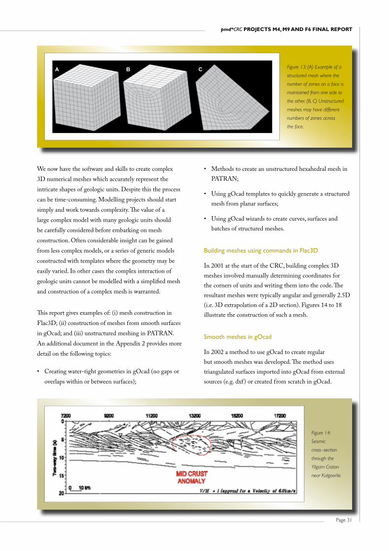
Page 31
pmd*CRC ProjeCtS M4, M9 and F6 Final rePort
• MethodstocreateanunstructuredhexahedralmeshinPATRAN;
• UsinggOcadtemplatestoquicklygenerateastructuredmesh from planar surfaces;
• UsinggOcadwizardstocreatecurves,surfacesandbatches of structured meshes.
Building meshes using commands in Flac3D
In 2001 at the start of the CRC, building complex 3D meshes involved manually determining coordinates for the corners of units and writing them into the code. The resultant meshes were typically angular and generally 2.5D (i.e. 3D extrapolation of a 2D section). Figures 14 to 18 illustrate the construction of such a mesh.
Smooth meshes in gOcad
In 2002 a method to use gOcad to create regular but smooth meshes was developed. The method uses triangulated surfaces imported into gOcad from external sources (e.g. dxf ) or created from scratch in gOcad.
We now have the software and skills to create complex 3D numerical meshes which accurately represent the intricate shapes of geologic units. Despite this the process can be time-consuming. Modelling projects should start simply and work towards complexity. The value of a large complex model with many geologic units should be carefully considered before embarking on mesh construction. Often considerable insight can be gained from less complex models, or a series of generic models constructed with templates where the geometry may be easily varied. In other cases the complex interaction of geologic units cannot be modelled with a simplified mesh and construction of a complex mesh is warranted.
This report gives examples of: (i) mesh construction in Flac3D; (ii) construction of meshes from smooth surfaces in gOcad; and (iii) unstructured meshing in PATRAN. An additional document in the Appendix 2 provides more detail on the following topics:
• Creatingwater-tightgeometriesingOcad(nogapsoroverlaps within or between surfaces);
Figure 13: (A) Example of a
structured mesh where the
number of zones on a face is
maintained from one side to
the other. (B, C) Unstructured
meshes may have different
numbers of zones across
the face.
Figure 14:
Seismic
cross–section
through the
Yilgarn Craton
near Kalgoorlie.

Page 32
Figure 17: Resultant Flac3D mesh.
Figure 16: Typical nature of code required
to build a complex mesh.
Figure 15:
Simplified
cross-section
based on
Figure 14. This
diagram contains
the coordinates
which are then
put into code
form (Figure 16).
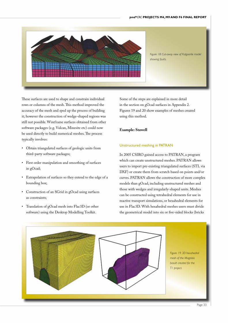
Page 33
pmd*CRC ProjeCtS M4, M9 and F6 Final rePort
Some of the steps are explained in more detail in the section on gOcad surfaces in Appendix 2. Figures 19 and 20 show examples of meshes created using this method.
Example: Stawell
Unstructured meshing in PATRAN
In 2005 CSIRO gained access to PATRAN, a program which can create unstructured meshes. PATRAN allows users to import pre-existing triangulated surfaces (STL via DXF) or create them from scratch based on points and/or curves. PATRAN allows the construction of more complex models than gOcad, including unstructured meshes and those with wedges and irregularly-shaped units. Meshes can be constructed using tetrahedral elements for use in reactive transport simulations, or hexahedral elements for use in Flac3D. With hexahedral meshes users must divide the geometrical model into six or five-sided blocks (bricks
These surfaces are used to shape and constrain individual rows or columns of the mesh. This method improved the accuracy of the mesh and sped up the process of building it; however the construction of wedge-shaped regions was still not possible. Wireframe surfaces obtained from other software packages (e.g. Vulcan, Minesite etc) could now be used directly to build numerical meshes. The process typically involves:
• Obtaintriangulatedsurfacesofgeologicunitsfromthird-party software packages;
• Firstordermanipulationandsmoothingofsurfacesin gOcad;
• Extrapolationofsurfacessotheyextendtotheedgeofabounding box;
• ConstructionofanSGridingOcadusingsurfacesas constraints;
• TranslationofgOcadmeshintoFlac3D(orothersoftware) using the Desktop Modelling Toolkit.
Figure 18: Cut-away view of Kalgoorlie model
showing faults.
Figure 19: 3D hexahedral
mesh of the Magdala
basalt created for the
T1 project.
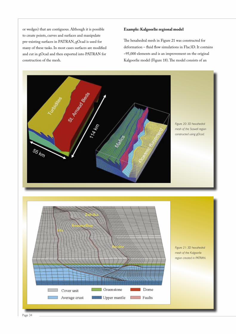
Page 34
Example: Kalgoorlie regional model
The hexahedral mesh in Figure 21 was constructed for
deformation – fluid flow simulations in Flac3D. It contains
~95,000 elements and is an improvement on the original
Kalgoorlie model (Figure 18). The model consists of an
or wedges) that are contiguous. Although it is possible to create points, curves and surfaces and manipulate pre-existing surfaces in PATRAN, gOcad is used for many of these tasks. In most cases surfaces are modified and cut in gOcad and then exported into PATRAN for construction of the mesh.
Figure 20: 3D hexahedral
mesh of the Stawell region
constructed using gOcad.
Figure 21: 3D hexahedral
mesh of the Kalgoorlie
region created in PATRAN.

Page 35
pmd*CRC ProjeCtS M4, M9 and F6 Final rePort
Example: Great Basin (Utah and Nevada)
The construction of the mesh for the Great Basin project (Figure 23) involved considerable manipulation of surfaces in gOcad, ensuring there were no gaps, overlaps or duplicate nodes where surfaces met. Because the model was designed for thermal – fluid flow simulation in the RT code it could be meshed using tetrahedral elements (as opposed to hexahedra, required for Flac3D). The
upper crustal cover unit (10km thick), a greenstone layer
(2km thick), an average crustal unit (the domain between
the greenstone and the Moho), lithospheric upper mantle,
four faults (Ida, Bardoc, Kunanalling and Zuleika) and a
thin, dome-shaped zone (assumed to be a detachment/
shear zone). Wedge-shaped units are represented
(e.g. between Zuleika and Bardoc Faults) which would
not have been possible to mesh in gOcad.
Figure 22: Cutaway image
of the Kalgoorlie regional
model created in PATRAN.
Figure 23: Tetrahedral mesh
constructed for the Great
Basin project (in PATRAN).
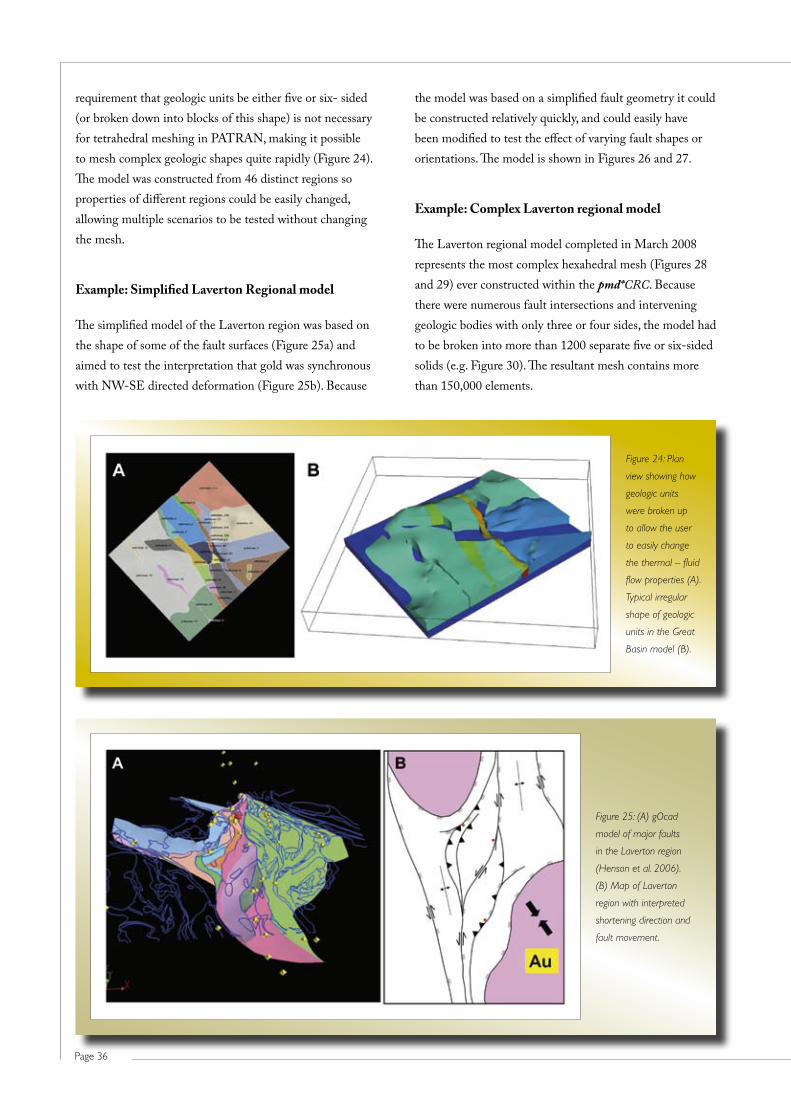
Page 36
the model was based on a simplified fault geometry it could be constructed relatively quickly, and could easily have been modified to test the effect of varying fault shapes or orientations. The model is shown in Figures 26 and 27.
Example: Complex Laverton regional model
The Laverton regional model completed in March 2008 represents the most complex hexahedral mesh (Figures 28 and 29) ever constructed within the pmd*CRC. Because there were numerous fault intersections and intervening geologic bodies with only three or four sides, the model had to be broken into more than 1200 separate five or six-sided solids (e.g. Figure 30). The resultant mesh contains more than 150,000 elements.
requirement that geologic units be either five or six- sided (or broken down into blocks of this shape) is not necessary for tetrahedral meshing in PATRAN, making it possible to mesh complex geologic shapes quite rapidly (Figure 24). The model was constructed from 46 distinct regions so properties of different regions could be easily changed, allowing multiple scenarios to be tested without changing the mesh.
Example: Simplified Laverton Regional model
The simplified model of the Laverton region was based on the shape of some of the fault surfaces (Figure 25a) and aimed to test the interpretation that gold was synchronous with NW-SE directed deformation (Figure 25b). Because
Figure 24: Plan
view showing how
geologic units
were broken up
to allow the user
to easily change
the thermal – fluid
flow properties (A).
Typical irregular
shape of geologic
units in the Great
Basin model (B).
Figure 25: (A) gOcad
model of major faults
in the Laverton region
(Henson et al. 2006).
(B) Map of Laverton
region with interpreted
shortening direction and
fault movement.
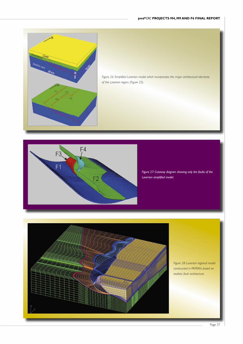
Page 37
pmd*CRC ProjeCtS M4, M9 and F6 Final rePort
Figure 27: Cutaway diagram showing only the faults of the
Laverton simplified model.
Figure 28: Laverton regional model
constructed in PATRAN, based on
realistic fault architecture.
Figure 26: Simplified Laverton model which incorporates the major architectural elements
of the Laverton region. (Figure 25).

Page 38
2002) which solve the equations of fluid flow, heat and mass transport, and chemical reactions on a 2D or 3D finite element mesh. The RT code simulates incompressible single-phase flow in a fluid-saturated porous medium and assumes thermodynamic equilibrium between chemical species in the fluid and solid phases.
Software
Software architecture
All modules used in the software are accessible through the Python programming language (www.python.org). The processingofheavycalculationsisdoneinCforefficiencypurposes and the Python wrapper facilitates ease of use.
Decomposing simulations in to time slices
An RT simulation is conceptually broken down into “time slices”. The quotes are needed because only some time slices represent elapsed time. Some time slices are artificial
References
Henson, P.A., Blewett, R.S., Champion, D.C., Goleby, B.R. and Czarnota, K., 2006. Towards a unified architecture of the Laverton region, WA. In: Barnicoat, A.C. and Korsch, R.J. (Eds.), Predictive Mineral Discovery Cooperative Research Centre – Extended abstracts from the April 2006 conference, Geoscience Australia Record 2006/07. Geoscience Australia, Canberra, Australia, p. 47–51.
2.3 The Reactive Transport Utility
Peter Hornby and Thomas Poulet
Introduction
The Reactive Transport (RT) utility developed by the pmd*CRC consists of a Gibbs minimisation solver (WinGibbs; Shvarov and Bastrakov 1999) coupled with a partial differential equation (PDE) solver (Fastflo4; Gross
Figure 30: Geometry of the Childe-Harold Fault within the
Laverton regional model. 124 solid volumes were required
for this fault alone. Each of these volumes was populated
with hexahedral elements.
Figure 29: Cut-away diagram of the
Laverton regional model showing
complex fault intersections.

Page 39
pmd*CRC ProjeCtS M4, M9 and F6 Final rePort
Subsequent time slices constitute the actual simulation with all process models used together. These time slices involve calculation of fluid fluxes and transport of heat and mass. Chemical updates are turned on if reactions are being modelled. More time slices can be added if the simulation is made of different phases in time, for example, intrusive events or sudden appearance of high permeability zones.
This concept of time line and time slices is a very useful abstraction mechanism and was consequently integrated to the Desktop Modelling Toolkit (see section 2.1).
FastfloFluidHeatChem interface
At the top level of the software stack is the FastfloFluidHeatChem interface which allows users to set input parameters by editing a Python dictionary. New users can control their simulations with simple intuitive descriptions (e.g. [‘fluidViscosity’] = {‘method’:’useEquationOfState’} or [‘fluidViscosity’] = {‘method’:’set’, ‘value’:0.001}), and expert users can benefit from the full power of a programming language and overwrite methods to implement their own algorithms.
There are many options to define parameters or functionalities, including creating save files that admit restarting of the simulation, or visualisation with Mayavi during the simulation run. These save files are standard python “pickle” files and can usually be used across multiple program versions.
modelling steps used to calculate initial conditions or boundary conditions or to update an aspect of the model, such as a changed boundary condition. A simulation comprises a succession of time slices, known as a time line. Each time slice is defined by boundary, domain and global conditions. Local data overwrites global data: information defined globally (for the whole model for a given time slice) is overwritten by information defined for each spatial domain of the mesh, which in turn is overwritten by boundary conditions.
A simulation is typically broken down into at least four time slices. The first initialises the temperature by solving the heat conduction equation to find the steady-state conductive geotherm. The second solves the pressure equation to establish the steady-state fluid pressure for the specified boundary conditions. The third time slice initialises pressure and temperature together. This sequential initialisation is needed because fluid properties and chemical equilibrium depend on pressure and temperature. However, the initial distributions of temperature and pressure are non-trivial if the top boundary of the model includes topography, if there are heat sources in the model (representing radioactive decay), or if different domains have different properties (e.g. permeability). Another time slice may be devoted to initialising the chemistry; that is, equilibrating the fluid and solid under the initial temperature and pressure conditions just calculated. Fluid density depends also on the concentration of dense tracers (representing salinity), so another time slice is needed if dense tracers are involved.
Figure 31: Software components and
their programming language.
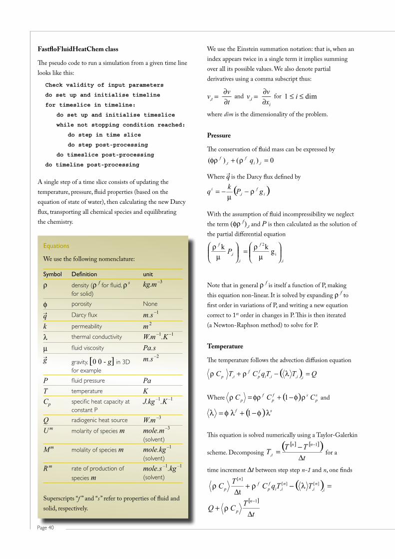
Page 40
We use the Einstein summation notation: that is, when an index appears twice in a single term it implies summing over all its possible values. We also denote partial derivatives using a comma subscript thus:
v,t =∂v and v,i =
∂v for 1 ≤ i ≤ dim∂t ∂xi
where dim is the dimensionality of the problem.
Pressure
The conservation of fluid mass can be expressed by
Where q➝ is the Darcy flux defined by
With the assumption of fluid incompressibility we neglect the term (φρ f ),t and P is then calculated as the solution of the partial differential equation
Note that in general ρ f is itself a function of P, making this equation non-linear. It is solved by expanding ρ f to first order in variations of P, and writing a new equation correct to 1st order in changes in P. This is then iterated (a Newton-Raphson method) to solve for P.
Temperature
The temperature follows the advection diffusion equation
Where sp
sfp
fp CCC 1 and
This equation is solved numerically using a Taylor-Galerkin
scheme. Decomposing tTT
Tnn
t
1
, for a
time increment ∆t between step step n-1 and n, one finds
0) ()( ,, iif
tf q
if
ii gP
kq ,
i
f
i
i
f
P,
i
2
,
, g k
k
QTTqCTCiiii
fp
ftp ,,,,
sf 1
tT
CQTTqCT
Cn
pi
ni
nii
fp
fn
p
1
,
][,
][,
][
t
tT
CQTTqCT
Cn
pi
ni
nii
fp
fn
p
1
,
][,
][,
][
t
FastfloFluidHeatChem class
The pseudo code to run a simulation from a given time line looks like this:
Check validity of input parameters
do set up and initialise timeline
for timeslice in timeline:
do set up and initialise timeslice
while not stopping condition reached:
do step in time slice
do step post-processing
do timeslice post-processing
do timeline post-processing
A single step of a time slice consists of updating the temperature, pressure, fluid properties (based on the equation of state of water), then calculating the new Darcy flux, transporting all chemical species and equilibrating the chemistry.
Equations
We use the following nomenclature:
Symbol Definition unit
ρ density (ρ f for fluid, ρ s for solid)
kg.m –3
φ porosity None
q➝ Darcy flux m.s –1
k permeability m 2
λ thermal conductivity W.m –1.K –1
µ fluid viscosity Pa.s
g➝ gravity, [0 0 - g] in 3D for example
m.s –2
P fluid pressure PaT temperature KCp specific heat capacity at
constant PJ.kg –1.K –1
Q radiogenic heat source W.m –3
U m molarity of species m mole.m –3 (solvent)
M m molality of species m mole.kg –1 (solvent)
R m rate of production of
species mmole.s –1.kg –1 (solvent)
Superscripts “f ” and “s ” refer to properties of fluid and solid, respectively.

Page 41
pmd*CRC ProjeCtS M4, M9 and F6 Final rePort
to the velocity is a product of the transverse dispersion coefficientmultipliedbythemagnitudeoftheflux.
Numerical problems
Advection-diffusion problems such as the solute and temperatureequationscanbedifficulttosolvenumerically.The act of forming a finite element or finite difference approximation can lead to implicit negative diffusion terms that may exceed the positive diffusion in the problem. This is especially true if the flow is advection dominated, and manifests itself as spatial oscillations in the quantity being transported. These oscillations tend to occur at places in the mesh where the concentration or temperature are rapidly changing functions of position. The solute transport problem generally suffers from this more than the temperature equation because the solute problem is generally more advection dominated. This is because solute is transported only in the fluid phase, while heat diffuses through both the solid and fluid. To combat this, a conventional approach has been taken called upwinding. See Appendix A at the end of this section for more details onthemethodusedandthecoefficientsexposedthroughthe interface for users to control this process.
Chemistry
The approach to chemistry is quite conventional, with some novel twists. It separates the transport and chemical updates into two steps, a procedure known as operator splitting. The chemical update is done using a Gibbs free energy minimisation procedure, WinGibbs (Shvarov and Bastrakov, 1999).
The principle is as follows: Given the transport equations for the fluid species, we form special linear combinations of these equations
Next, we suppose all the fluid species have the same mean velocity (the solvent velocity) and the same diffusion coefficient.Thismaynotbethecase,butmostreactivetransport codes assume this because doing otherwise requires consideration of charge balance and species interaction with electric fields. Defining the quantity
n
mnm
f
mi
mjij
mii
mt
nm RUDUqU
,,,,
n
mnm
n UT
Mass transport
The conservation of mole number written in terms of molality is (Steefel, 1992)
This equation, converted to molarity (because the diffusive flux is driven by a volumetric concentration) is:
Using the conservation of fluid mass
one finds
If there are sources or sinks for the fluid mass (e.g. chemical reactions) this equation requires a simple modification to the right-hand side. This is not done here, since we assume incompressible flow anyway. Compressible flow is considered in the coupling with deformation (see section 2.5).
Next, suppose ρ f is a slowly varying function of space and time, so its derivatives are small. Then we obtain
Following common practice, the transport of all chemical species and inert tracers is calculated using the same advection diffusion equation that is used for temperature calculation with an anisotropic dispersion and a different velocity. In the current code, we use the equation:
The total dispersion Dij is the sum of an isotropic molecular diffusion term and a dispersion term. It is determinedbythreecoefficients:amoleculardiffusioncoefficient,alongitudinaldispersionlengthandatransversedispersion length. The magnitude of the dispersion term in the direction of the molecular velocity is a product of thelongitudinaldispersioncoefficientandthemagnitudeof the flux. The magnitude of the dispersion perpendicular
mf
ijmf
ijm
if
t
mf RMDMqM,,,
)(
mf
i
mjij
mit
m RUDUqU,,,
0) ()( ,, iif
tf q
mf
i
mjij
mii
fmt
f RUDMqM,,,,
mf
i
mjij
mii
mt RUDUqU
,,,,
mfi
mjijm
iim
t RUD
Uq
U ,,
,,

Page 42
For each node:
1. Take the number of moles of each species and transfer those numbers, and the temperature and pressure at the finite element node, into an object called a ChemicalSystem.
2. Bring the ChemicalSystem to equilibrium using a ChemicalSolver. In this case the ChemicalSolver uses WinGibbs as follows:
a. Convert the species mole numbers into a bulk composition specified by moles of chemical elements and moles of water.
b. Pass this bulk composition to WinGibbs.
c. Take the speciation calculated by WinGibbs and set it back into the ChemicalSystem.
3. Transfer the ChemicalSystem object’s mole numbers back to the finite element node.
At this stage we have a finite element mesh in chemical equilibrium. During the equilibration, the volume of matter at each node, and the solid and fluid volume fractions may have changed. The mole numbers are then adjusted to bring the volume back to one litre, and solid/fluid volume fractions back to their specified values. This is done in the obvious way, preserving the mineral volume fractions and fluid concentrations, so equilibrium is not perturbed.
This mesh composition can now be used as the initial chemical state of the model. This procedure can also be used to construct compositions to be used to provide values for boundary conditions on chemical composition. For example, the above procedure can be used to prepare a model state that is saturated in gold at a set of boundary nodes. One simply adds gold to nodes close to the boundary and performs the above procedure to get a fluid saturated in gold at those nodes. Then one removes the gold from the solid matrix, and repeats the procedure to calculate a second composition to be used as the initial condition. Now the model can be run using the latter composition as the initial composition, but using the gold saturated solution for imposing boundary condition on some segment of the boundary, e.g. where a fault intersects the boundary. This is the philosophy for controlling incoming fluid compositions. It fits easily in the time line approach to constructing simulations.
we get
by linearity. The trick is then to choose the ν nm so that
n
mnmR contains only rates due to
precipitation-dissolution reactions. Such a T n is referred to as an aqueous reaction extent invariant. One choice is to take T n to be the total concentrations of solute basis species. In our code, we make a different choice. We take the ν nmtobethecompositionalstoichiometriccoefficientof chemical element n in species m. T n is therefore the concentration of chemical element n in the fluid, and is independent of the extent of chemical reactions between fluid species. It is also positive, allowing checking for unstable spatial oscillations caused by under-diffusion.
With the above as background, we can outline the algorithm used to model reactive transport. Firstly, there is the stage of specifying the chemical composition of the model:
1. A one-litre container is associated with each node of the finite element mesh. This is novel. Most other codes associate composition with elements rather than nodes.
2. Fluid and solid volume fractions are also associated with these containers at each node. This is specified by assigning a porosity.
3. A mineral assemblage is specified for each node, usually as fractions of solid volume occupied by each mineral.
4. The fluid volume fraction is filled with water.
5. Solute species concentrations are set in the fluid.
At this stage, there is associated with each node a given number of moles of each mineral, solvent and solute species in the chemical system. Only these mole numbers are kept. From here on, all concentrations, volumes etc. are derived from the actual number of moles, temperature and pressure. The chemical compositions at the nodes are generally not in equilibrium at this stage.
We assume we have calculated the initial temperature and pressure. Given that, we do the following initialisation of the chemical composition:
n
mnm
f
i
njij
nii
nt RTDTqT
,,,,

Page 43
pmd*CRC ProjeCtS M4, M9 and F6 Final rePort
• Ourcodeisnotmulti-threaded(apartfromthechemistry calculation) and so cannot take advantage of multiple processors if available.
• Thecodeislimitedtosinglephaseflow.
• Thechemistrycalculationsdonotaccountforreactionkinetics or latent heat.
• Fluidcompressibilityisignored;volumetricflowandchemical effects due to fluid creation/destruction are ignored.
Some of these limitations are due to the choice of Fastflo4 as our PDE solver; these issues will be resolved in a future version of the code based on eScript (Gross, Cumming et al. 2007). This version is being developed and will be able to be run in parallel on multiple processors, handle the symmetry problem better, deal with flux boundary conditions correctly, and let users define the order in which to set boundary conditions. Preliminary tests show promising results. The Elder problem presented in section 2.4 was run with the current code and this new code on the same machine using one processor. The outcome is encouraging. The new code showed a 56% decrease in run time (more than twice as fast), used 15% less memory and produced symmetrical results (Figure 32).
Work to couple mechanical deformation with the RT code has already started (see section 2.5). Future steps will include using the enthalpy equation instead of the temperature equation as a first step toward enabling simulation of phase changes and multi-phase flow.
Appendix A: Upwinding
Advection-diffusion problems such as the solute and temperature equations can be hard to solve numerically. Forming a finite element or finite difference approximation can lead to implicit negative diffusion terms that may exceed the positive diffusion in the problem. This is especially true if the flow is advection dominated and manifests as spatial oscillations in the quantity being transported. These oscillations tend to occur at places in the mesh where the concentration or temperature are rapidly-changing functions of position. The solute transport problem generally suffers from this more than the temperature equation because it is generally more advection dominated.
Finally, there is the simulation itself:
1. For each node, convert the liquid phase into solvent moles and solute element moles.
2. For each node, calculate total chemical element concentrations T n.
3. Transport the chemical elements using the advection-diffusion equation.
4. Check for negative T n ( = numerical instability).
5. For each node, convert T n back to moles of solute elements.
6. For each node, convert moles of solute elements to a solute bulk composition in terms of moles of solute basis species.
7. For each node, pass this composition to a ChemicalSystem, and call a ChemicalSolver to speciate it.
The double step in converting to the bulk composition of solutes in terms of elements into a bulk composition in terms of basis solute species allows support for solvers other than Gibbs free energy minimisers.
Benchmarks
The algorithms for heat and solute transport have been validated against analytical and numerical solutions. Chemistry has also been validated against numerical solutions obtained using other codes e.g. Shemat. See section 2.4 for details.
Limitations and further developments
The current version of the code includes at least the following limitations:
• Fastflo4doesn’thandleproperlyboundaryconditionssetas fluxes;
• Fastflo4producesasymmetricresultswhensolvingthetransport equation;
• Userscannotcontroltheorderinwhichtheboundaryconditions are set, since this information cannot be propagated to Fastflo4. Users have to check manually edges and corner nodes of their models to verify how boundary conditions have been applied.

Page 44
The number Kxv
Pe2
is often called the local Peclet number. If Pe > 1 one runs the risk of spatial oscillations in the solution in regions of sharp variations of U. Historically, it was discovered that using an “upwind” difference for the advection term cured this problem. For ν > 0 the flow is from left to right, and so a less accurate approximation to the advection term was introduced that transmitted information from left to right.
However, this can be re-written as a central difference as follows
and we see that the effect of the upwind finite difference is to add an extra diffusion term. It is interesting to note this extra diffusion term is of the same form as the extra diffusion added to account for dispersion, a fact that is probably not entirely coincidence. This upwind method turns out to be over-diffusive, suggesting one might introduce a parameter ξ ∈ [0,1] to adjust this extra diffusion, like so
022 1111 iiiii UUU
xv
KUU
02
2
111
x
UUUK
xUU
viiiii
02
2 2
1111
x
UUUxvK
x
UUv
iiiii
02
2 2
1111
x
UUUxvK
x
UUv
iiiii
To combat this numerical instability, a conventional approach called upwinding has been taken. The name is derived from early finite difference methods, though many variations have been developed since. To explain it we have implemented as simply and briefly as possible a simple 1D advection diffusion equation. We also suppose the space dimension has been scaled so the space coordinate x is between 0 and 1. The equation for steady state flow, (time derivatives are zero) for constant velocity ν and diffusivity K is
In addition, we add the boundary conditions (keeping it simple) U(0) = 0 U(1) = 1
The solution to this is
So, for Kv
large we get a sharp variation near x = 1. Such
sharp changes are typical of, say, fast hot fluid flows across the top surface of a model, where the boundary temperature is fixed at a value very different from the impinging fluid. Taking a second order accurate (central) finite difference in x, using a grid of spacing ∆ x one obtains
or
02
2
dxUd
KdxdU
v
1exp
1exp
)(
Kv
Kvx
xU
02
2 2
1111
x
UUUK
xUU
viiiii
Figure 32: Asymmetry problems using the current code (A) are fixed using
the eScript version of the code (B).
Page 45
pmd*CRC ProjeCtS M4, M9 and F6 Final rePort
References
Bear, J., 1979. Hydraulics of groundwater. McGraw-Hill, New York, 569p.
de Marsily, G., 1986. Quantitative hydrogeology: Groundwater hydrology for engineers. Academic Press, Orlando, Florida, 464p.
Dullien, F.A.L., 1979. Porous media transport and pore structure. Academic Press, New York.
Gross, L., 2002. ‘Fastflo4’. CSIRO Mathematical and Information Sciences Software.
Gross, L., Cumming, B. et al., 2007. A python module for PDE-based numerical modelling: Applied parallel computing. State of the Art in Scientific Computing. Springer, Berlin/Heidelberg, 4699, pp. 270–279.
Shvarov, Y.V. and Bastrakov, E.N., 1999. AGSO record. Australian Geological Survey Organisation, 25, p. 61.
Steefel, C.I., 1992. Coupled fluid flow and chemical reaction: Model development and application to water-rock interaction. PhD thesis, Yale University.
2.4 Validating Heat and Tracer Transport in the Reactive Transport Utility
Heather A. Sheldon
Introduction
Transport of heat and solutes/tracers by advection and diffusion are important components of the pmd*CRC’s Reactive Transport (RT) code (Section 2.3). The transport algorithms were validated by comparing the numerical solution from RT with analytical solutions for simple problems (1D advective-diffusive transport of heat or tracer, and the onset of free thermal convection), and with numerical solutions from other codes for more complex problems (the Elder problem and a thermohaline convection problem). This paper summarises the outcomes of the validation tests; full details can be found in Appendix 2.
It turns out, rather spectacularly, that the choice
results in a solution to the finite difference equation that is exactly equal to the actual solution of the differential equation. Unfortunately, this is only true in 1D, and for constant velocity, diffusion, uniform mesh etc. Nevertheless the result is a good guideline for combating numerical under-diffusion. With this as background we can report the upwinding method we have used.
In essence we add a diffusion term of the magnitude
However,thisstatementharboursseveraldifficultiesin2D and 3D. Firstly, the “size” of a finite element (h) is estimated as the mean chord length of a finite element in the direction of the Darcy flux q➝. The scalar diffusion K appearing in the calculation of Pe is taken as Kij ni nj where Kij is the diffusion term accounting for porosity, heat capacities or other terms that may find their way into the effective diffusivity. The unit normal vector ni points in the direction of the flux. The extra diffusion is then added only in the direction of flow, that is, a term jinn
hvPe
2)(
is added to Kij.
The advective speed ν is similarly taken to be the magnitude of the Darcy flux, corrected for terms that may have found their way into the advection term. Finally, we use the approximation
For the diffusion correction factor. The constant k can be adjusted by the user. Its default value is unity. This scheme needs to be reviewed and possibly modified in concert with a review of the dispersion calculations and the transport equation itself (Bear 1979; Dullien 1979; de Marsily 1986).
PePePe
1)coth()(
2)(
hvPe
2
2
9)(
PePe
kPe

Page 46
Results
1D Diffusive Transport (steady state)
RT reproduces the steady-state solution for one-dimensional diffusive transport of heat (with a source term) with a high level of accuracy. The largest errors occurred on triangular and tetrahedral meshes with a heat flux boundary condition, but the maximum error was still small (< 0.05%).
RT reproduces the steady-state solution for one-dimensional diffusive transport of tracer with an extremely high level of accuracy. The global and maximum errors were ~4 x 10⁻¹⁰ and ~7 x 10⁻¹⁰, respectively, on all mesh types.
1D Advective-Diffusive Transport (steady state)
RT reproduces the steady-state solution for one-dimensional advective-diffusive transport of heat or tracer with a high level of accuracy. Triangular and tetrahedral meshes produce larger errors than rectangular or hexahedral meshes with the same element size. For a given Pe, the error is reduced by more than two orders of magnitude if Pelocal is reduced by one order of magnitude (by refining the mesh). Upwinding is needed to ensure spatial stability if Pelocal is large; for example, the numerical solution displays spatial instability with Pelocal = 5 and U = 0, but the instability is resolved if Pelocal is reduced to 0.5 or if U is increased to 1.
1D Advective-Diffusive Transport (transient)
RT reproduces the transient (time-dependent) solution for one-dimensional advective-diffusive transport of heat and tracer with an acceptable level of accuracy, depending on the local Peclet number, Courant overstep and upwinding (Figure 33). Upwinding is needed to maintain stability if Pelocal is high, but this introduces numerical dispersion. Increasing the Courant overstep above 1 has a similar effect. If accuracy is important, the mesh density should be chosen to yield Pelocal < 2 (such that upwinding is not needed) and the Courant overstep should be set to 0.1 or less.
Onset of free thermal convection
Classical analysis predicts free thermal convection occurs when the Rayleigh number, Ra, meets or exceeds a critical value. This value depends on the problem’s geometry and boundary conditions (Nield and Bejan, 1992).
Concepts
For tests involving comparison with an analytical solution, the accuracy of the numerical solution was assessed by calculating the global error, defined as:
nananum
H
XXXXn
E0
1 (1)
where X is the transported quantity (i.e. temperature or tracer concentration), X0 and XH are the values of X at the base and top of the column, subscripts num and ana indicate the numerical and analytical solutions, and n is the number of nodes in the finite element mesh. The maximum error was also recorded, this being the largest error at any single point on the mesh.
Tests were run on a variety of meshes, including 2D meshes comprising rectangular or triangular elements, and 3D meshes comprising hexahedral or tetrahedral elements.
The analytical solutions for advective-diffusive transport are expressed in terms of the global Peclet number, Pe, which reflects the balance between advection and diffusion over the model’s length. Stability and accuracy of the numerical solution depends on the local Peclet number, Pelocal, which reflects the balance of advection and diffusion over the length of a single element in the mesh.
RT uses an implicit solver which ensures the numerical solution is temporally stable for an arbitrarily large timestep. This means problems spanning a long time period can be solved in a small number of steps, but at the expense of accuracy. The loss of accuracy is characterised by “numerical dispersion” (smoothing of gradients in the transported quantity; this is particularly apparent where there should be sharp changes across a few nodes, which is typically the case in high Pe scenarios). The two options for setting the timestep in RT are: (i) Specifying a fixed timestep, ∆t; or (ii) specifying the Courant overstep, α, such that ∆t = αh/v, where h is the length of a mesh element in the direction of flow and v is the transport velocity. The solution is expected to be accurate for α ≤ 1.
The numerical solution for an advection-diffusion problem is expected to display spatial instability if Pelocal > 2 (e.g. Clauser, 2003). RT provides upwinding (represented by the upwind parameter, U ) to prevent such instabilities, but upwinding causes numerical dispersion.
The effects of varying timestep and upwinding are explored in the validation tests.

Page 47
pmd*CRC ProjeCtS M4, M9 and F6 Final rePort
of free thermal convection at the critical Rayleigh number on a mesh composed of uniform rectangular or hexahedral elements. However, RT predicts convection at sub-critical Rayleigh number on a mesh composed of triangular elements (Figure 34).
The onset of free thermal convection was tested with two sets of boundary conditions: (i) Fixed temperature and impermeable at the top and base; or (ii) Fixed heat flux and impermeable at the base, and fixed temperature and fluid pressure at the top. RT predicts correctly the onset
Figure 34: Temperature histories at six points across the model’s centre. Temperature evolves to a new steady-state value if convection occurs. Note
occurrence of convection at Ra < Rac on the triangular mesh.
Figure 33: Numerical and analytical solutions for advective-conductive heat transport illustrating effects of varying Pelocal, Courant overstep (Co), upwinding,
and dimensionless time (t’). Co = 0.1, U =0 and t’ = 0.2 unless otherwise specified. Note spatial instability in (A) and (B), and numerical dispersion in all
except (D).

Page 48
The solution becomes asymmetric and more diffusive
with decreasing mesh resolution or increasing timestep
(Figure 35).
Thermohaline convection
This test involves advective-diffusive transport of heat and
a dense tracer (representing salt). It explores the evolution
of temperature and tracer concentration (salinity) in a
2.5km square box containing a smaller region of fluid that
is initially more or less buoyant than the surrounding fluid.
The solution produced by RT is qualitatively correct and
similar to that produced by Geiger et al. (2006), however it
tends to become asymmetric (Figure 36).
The Elder problem (flow driven by a dense tracer)
In the Elder problem (Elder, 1967), a saline fluid 20% denser than pure water sinks downwards from a source region occupying part of the top boundary of a rectangular domain. Flow is driven purely by the variation in fluid density imparted by the salt; temperature and fluid pressure have no effect on fluid density. All boundaries are impermeable, except at the top corners where the fluid pressure is fixed.
RT produces a solution to the Elder problem that is very similar to those obtained using other codes (e.g. Clauser, 2003; Geiger et al., 2006), as long as the mesh resolution issufficientlyfineandthetimestepsufficientlysmall.
Figure 36: Solutions to the
thermohaline convection
problem with initially
positive (top) and negative
buoyancy (bottom) in the
internal box. Left to right:
Tracer concentration, fluid
flow vectors, fluid density,
temperature. Note the
development of asymmetry.
Figure 35: Solutions to the Elder
problem at 2, 10 and 20 years
on coarse, medium and fine
meshes (triangular elements), using
timesteps of 0.1 and 0.01 years.
Contours show tracer concentration
in 0.1 intervals from 0.0 to
1.0 kg/m3.

Page 49
pmd*CRC ProjeCtS M4, M9 and F6 Final rePort
presented in this section are extensions of the RT utility, which was described in detail in section 2.3. This work is of importance for the future direction of the RT code. However, it is still at the proof-of-concept stage.
We use the Einstein summation notation: that is, when an index appears twice in a single term it implies we are summing over all its possible values. We denote partial derivatives using a column subscript:
v,t =∂v and v,i =
∂v for 1 ≤ i ≤ dim∂t ∂xi
where dim is the dimensionality of the problem. More details about the following equations can be found on the Twiki page CouplingMechRT on the Swframe web.
Equations
All equations derive from those used in the RT code. Only the pressure and temperature equations differ and are presented here.
We use the following nomenclature:
Symbol Definition unit
ρ density (ρ f for fluid, ρ s for solid)
kg.m –3
φ porosity None
q➝ Darcy flux (in co-moving frame)
m.s –1
k permeability m 2
λ thermal conductivity W.m –1.K –1
µ fluid viscosity Pa.s
g➝ gravity, [0 0 g] in 3D for example
m.s –2
P fluid pressure PaT temperature KCp specific heat capacity J.kg –1.K –1
Q radiogenic heat source W.m –3
u➝ velocity in the Eulerian frame
m.s –1
v➝ velocity of Eulerian frame in rest frame
m.s –1
Superscripts “f ” and “s ” refer to properties of fluid and solid, respectively.
Conclusion
Validation tests have shown the RT utility can be used to simulate advective-diffusive transport of heat and/or tracer, with accuracy depending on Pelocal, Courant overstep and upwinding as expected. The only significant problems are: (i) the code predicts free convection at sub-critical Rayleigh number on triangular meshes; and (ii) solutions to symmetrical problems tend to become asymmetric. It is expected these problems will be resolved when the code is transferred from Fastflo to Escript.
References
Clauser, C., 2003. Numerical simulation of reactive flow in hot aquifers: SHEMAT and Processing SHEMAT. Springer, Berlin, 332 pp.
Elder, J.W., 1967. Transient convection in a porous medium. Journal of Fluid Mechanics, 27, p. 609–623.
Geiger, S., Driesner, T., Heinrich, C.A. and Matthäi, S.K., 2006. Multiphase thermohaline convection in the Earth’s crust: II. Benchmarking and application of a finite element – finite volume solution technique with a NaCl-H2O equation of state. Transport in Porous Media, 63, p. 435–461.
Nield, D.A. and Bejan, A., 1992. Convection in porous media. Springer-Verlag, New York.
2.5 Coupling Reactive Transport with Deformation
Thomas Poulet and Peter Hornby
Introduction
The Reactive Transport (RT) utility solves the equations of fluid flow, heat and mass transport, and chemical reactions, but not mechanical deformation. This document describes an approach for coupling the Abaqus software (Hibbit, Karlsson et al., 2003) for simulating mechanical deformation with the RT code for all other processes. There is flexibility to decide which code handles which processes as both handle heat transfer, for example. For now, most of the calculations are done in RT and Abaqus has been used for deformation only. All equations and software

Page 50
• fluiddensityatfirstorderin∆P, ignoring its dependency in T:
Each step from [n-1] to [n] gets broken down in several iterations on m such that
P [n,m] = P [n,m–1] + ∆P m with P [n,0] = P [n–1]
The equation to solve for ∆P m then becomes
Temperature
The temperature follows the advection diffusion equation like in the RT code, but differs from it since the fluid is now considered compressible and we take into account the mechanical velocity v➝. That equation becomes
Where sf CpCpCp 1 and
This equations gets solved numerically using a Taylor-Galerkin scheme by decomposing
for a time increment dt between step n −1 and n and using property values from the previous step[n − 1].
PP
nnnfn
]1[]1[][][
]1[]1,[]1,[
]1[]1,[]1,[],[]1[],[ nmnmmn
nmnmnmnnmn PP
]1[]1,[]1,[
]1[]1,[]1,[],[]1[],[ nmnmmn
nmnmnmnnmn PP
0 1 ,
1]2-[n
,
]1,[,
1]-[n
,]1[]1,[
]1,[
i
i
i
mi
mniii
nmnmmn
gk
tPPk
tvtPP
0 1 ,
1]2-[n
,
]1,[,
1]-[n
,]1[]1,[
]1,[
i
i
i
mi
mniii
nmnmmn
gk
tPPk
tvtPP
QTTvCpTqCpTCpiiiiiit ,,,
f
,
f,
QTTvCpTqCpTCpiiiiiit ,,,
f
,
f,
sf 1
dt
TTT
nn
t
1
,
From Eulerian to Lagrangian frame
If we consider a quantity X then its conservation can be written in the Eulerian frame as
where u➝ is the velocity in the Eulerian frame and RX is the production rate of X. If this Eulerian frame is moving with a velocity v➝ in the Euclidian “rest” frame we get the Lagrangian formulation
Note R LX is the rate of formation in the Lagrangian frame and R EX the rate of formation in the Eulerian frame. R LX applies to the volume which is co-moving with the frame (and might be deforming in the Euclidian “rest” frame). See Twiki page Pmdcrc.FourDTwoPhaseMechanics for more details.
Pressure
The main difference from the RT code is that the pore fluid is now considered to be compressible and we take into account the mechanical velocity v➝. The conservation of mass can be expressed as
qi represents the real Darcy flux and vi the mechanical velocity, so qi − φ vi represents the Darcy flux for the reactive transport in the co-moving frame and we’ll name it ~qi = qi − φ vi
By definition if
ii gPk
q~ so the mass
conservation equation becomes
To solve this equation numerically we make these assumptions between step n-1 and n:
• useφ, µ and k from the previous time step
• timederivativetxx
xnn
t
]1[][
,
• pressuretermatfirstorderP [n] = P [n–1] + ∆P
EXiit RXuX ,, )(
LXiiiiit RvuXXvX ,,, )(
0 )( ,,, iiif
iif
tf vqv
0)(,
2
,
,,,
i
i
f
i
i
f
iif
tf g
kP
kv
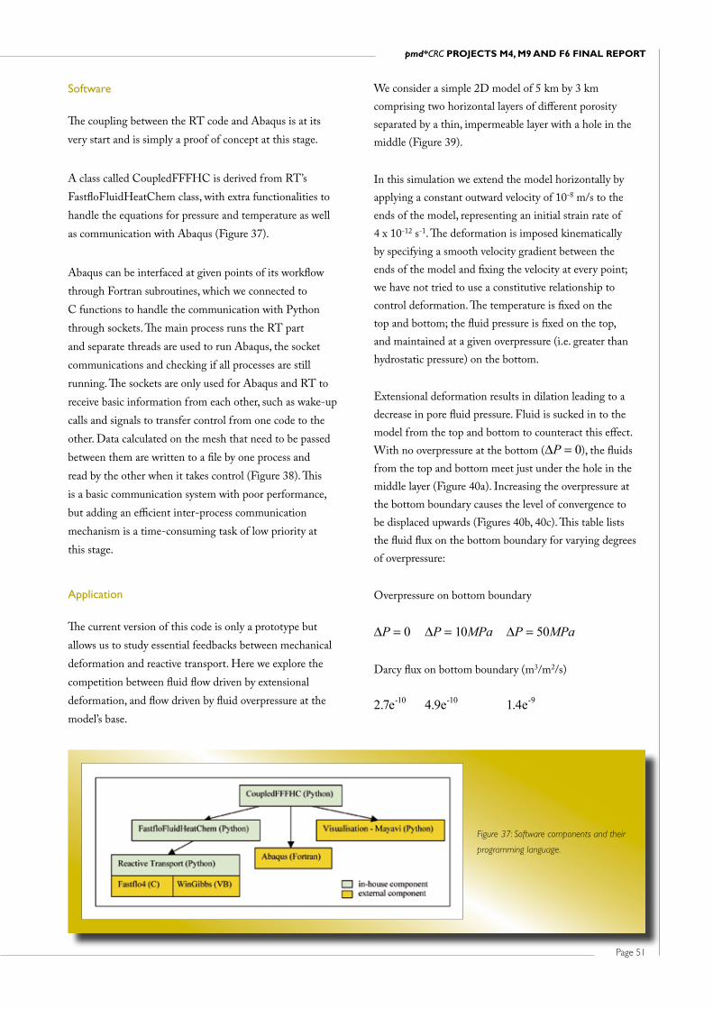
Page 51
pmd*CRC ProjeCtS M4, M9 and F6 Final rePort
We consider a simple 2D model of 5 km by 3 km comprising two horizontal layers of different porosity separated by a thin, impermeable layer with a hole in the middle (Figure 39).
In this simulation we extend the model horizontally by applying a constant outward velocity of 10-8 m/s to the ends of the model, representing an initial strain rate of 4 x 10-12 s-1. The deformation is imposed kinematically by specifying a smooth velocity gradient between the ends of the model and fixing the velocity at every point; we have not tried to use a constitutive relationship to control deformation. The temperature is fixed on the top and bottom; the fluid pressure is fixed on the top, and maintained at a given overpressure (i.e. greater than hydrostatic pressure) on the bottom.
Extensional deformation results in dilation leading to a decrease in pore fluid pressure. Fluid is sucked in to the model from the top and bottom to counteract this effect. With no overpressure at the bottom (∆P = 0), the fluids from the top and bottom meet just under the hole in the middle layer (Figure 40a). Increasing the overpressure at the bottom boundary causes the level of convergence to be displaced upwards (Figures 40b, 40c). This table lists the fluid flux on the bottom boundary for varying degrees of overpressure:
Overpressure on bottom boundary
∆P = 0 ∆P = 10MPa ∆P = 50MPa
Darcy flux on bottom boundary (m3/m2/s)
2.7e-10 4.9e-10 1.4e-9
Software
The coupling between the RT code and Abaqus is at its very start and is simply a proof of concept at this stage.
A class called CoupledFFFHC is derived from RT’s FastfloFluidHeatChem class, with extra functionalities to handle the equations for pressure and temperature as well as communication with Abaqus (Figure 37).
Abaqus can be interfaced at given points of its workflow through Fortran subroutines, which we connected to C functions to handle the communication with Python through sockets. The main process runs the RT part and separate threads are used to run Abaqus, the socket communications and checking if all processes are still running. The sockets are only used for Abaqus and RT to receive basic information from each other, such as wake-up calls and signals to transfer control from one code to the other. Data calculated on the mesh that need to be passed between them are written to a file by one process and read by the other when it takes control (Figure 38). This is a basic communication system with poor performance, butaddinganefficientinter-processcommunicationmechanism is a time-consuming task of low priority at this stage.
Application
The current version of this code is only a prototype but allows us to study essential feedbacks between mechanical deformation and reactive transport. Here we explore the competition between fluid flow driven by extensional deformation, and flow driven by fluid overpressure at the model’s base.
Figure 37: Software components and their
programming language.

Page 52
Figure 39: Initial porosity.
Figure 38: Sequence diagram for coupling
RT and Abaqus.

Page 53
pmd*CRC ProjeCtS M4, M9 and F6 Final rePort
Thee following developments were made for the FreeGs information system during the CRC’s second stage:
1. Incorporation of the new Equation of State to calculate thermodynamic properties of aqueous neutral species (e.g. H2 (aq), H2S (aq), etc);
2. An option to add incomplete thermodynamic data sets for reference and comparative purposes (i.e., for species, where only fragmental thermodynamic information is available);
3. Incorporation of DOI (digital object identifiers) into Geoscience Australia’s GeoRef and FreeGs databases to link FreeGs literature references to the original refereed journal publications;
4. Development of experimental access to the system as a web-service using XML.
Notes on FreeGs technical implementation
The technical implementation of the current FreeGs system comprises a set of Plain Old Java Objects (POJOs) that handle database access, session management and calculations needed to service the application. It was designed and implemented using the Model/View/Controller (MVC) methodology and the object-oriented technique permits effortless addition of new calculation algorithms. Most algorithms were extracted from the UNITHERM program of the HCh package for geochemical modelling (Shvarov and Bastrakov, 1999), complemented by the algorithms of the NonElectrolytes program (Akinfiev and Diamond, 2003).
The current technical implementation is illustrated by Figure 41. This simplified diagram shows the essential processing aspects of the web application. Data entry and
References
Hibbit, H. D., B. I. Karlsson, et al. (2003). ABAQUS Theory manual, Version 6.4.1. Pawtucket, RI (USA), Hibbit, Karlsson and Sorrenson Inc.
2.6 Virtual Centre for Geofluids
Evgeniy Bastrakov, Terry Mernagh and Dale Percival
Introduction
For background on the Virtual Centre for Geofluids (VC), its components and functionality readers are referred to F1-F2 and F3 final project reports of the pmd*CRC. The VC provides a one-stop web store of theoretical and empirical data for geochemical modelling community. It consists of two information systems: FreeGs, an on-line thermodynamic database plus integrated applications; and FIncs, an on-line fluid inclusion database plus applications to calculate fluid properties.
During the first stage of the pmd*CRC, the VC was mostly functioning in maintenance mode. The project’s fluid inclusion component (inherited from the Stage 1 F3 project) was incorporated in the Modelling project. The additions and changes to FreeGs and FIncs are summarised below.
FreeGs
The in-depth specifications and functionality of the FreeGs information system can be found at:
www.ga.gov.au/minerals/research/methodology/geofluids/freegs_reports_help.jsp
Figure 40: Fluid
flux magnitude
and streamlines
after 1000 years
of extension, with
∆P = 0, ∆P = 10MPa
and ∆P = 50MPa
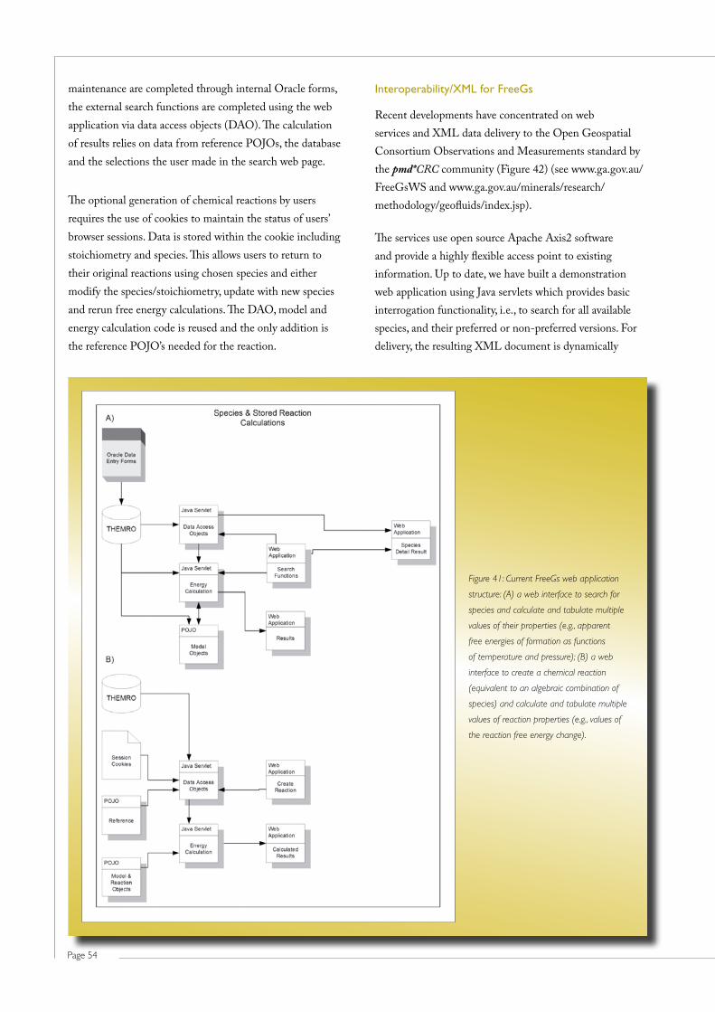
Page 54
Interoperability/XML for FreeGs
Recent developments have concentrated on web services and XML data delivery to the Open Geospatial Consortium Observations and Measurements standard by the pmd*CRC community (Figure 42) (see www.ga.gov.au/ FreeGsWS and www.ga.gov.au/minerals/research/methodology/geofluids/index.jsp).
The services use open source Apache Axis2 software and provide a highly flexible access point to existing information. Up to date, we have built a demonstration web application using Java servlets which provides basic interrogation functionality, i.e., to search for all available species, and their preferred or non-preferred versions. For delivery, the resulting XML document is dynamically
maintenance are completed through internal Oracle forms, the external search functions are completed using the web application via data access objects (DAO). The calculation of results relies on data from reference POJOs, the database and the selections the user made in the search web page.
The optional generation of chemical reactions by users requires the use of cookies to maintain the status of users’ browser sessions. Data is stored within the cookie including stoichiometry and species. This allows users to return to their original reactions using chosen species and either modify the species/stoichiometry, update with new species and rerun free energy calculations. The DAO, model and energy calculation code is reused and the only addition is the reference POJO’s needed for the reaction.
Figure 41: Current FreeGs web application
structure: (A) a web interface to search for
species and calculate and tabulate multiple
values of their properties (e.g., apparent
free energies of formation as functions
of temperature and pressure); (B) a web
interface to create a chemical reaction
(equivalent to an algebraic combination of
species) and calculate and tabulate multiple
values of reaction properties (e.g., values of
the reaction free energy change).

Page 55
pmd*CRC ProjeCtS M4, M9 and F6 Final rePort
To prove the concept of ‘many user interfaces, single
data source’ and ‘standards based web service’, we have
developed a stand-alone Java web start application
providing the same functionality of POST requests via the
web. Validation and processing is performed by Java code
according to an internally-held XML Schema Document
(XSD). This ensures submitted requests make sense to the
processing application.
The SpeciesHandler code contains public validation
and processing methods for XML/String queries. The
demonstration application uses these directly; the web
application uses them indirectly through the doGet/doPost
methods. Using the Axis2 framework, which incorporates
the Axiom XML model, SOAP messages with pre-defined
FreeGs query elements are generated on the fly and sent to
the Axis2 processing engine.
processed into html using a simple stylesheet. The use of a web application and Java servlets restrict the structure of SQL requests that the POJO is required to process to finite values. It also provides a level of security because malicious SQL cannot be injected into web form text fields. More advanced functionality using http POST, allows users to pass in an XML structured request that will be validated and processed according to the used XML element tags:
<?xml version=”1.0” encoding=”UTF-8” ?>
<frgs:Request xmlns:frgs=”http://www.
ga.gov.au/namespaces/FreeGs/0.1”>
<elementSearch>
<Preferred>Y</Preferred>
<ElementList>Na,Cl</ElementList>
</elementSearch>
</frgs:Request>
Figure 42: Example FreeGs web service.

Page 56
to each fluid inclusion, the classification systems used for the fluid inclusions (e.g., inclusion type, inclusion class and inclusion system), or on individual parameters in the database. Users can also search for records entered since a certain date, or updated since a certain date, or for inclusions associated with a particular paragenetic stage of ore deposit evolution. The search fields are combined with the Boolean logical “AND” operator. Each search returns a list of relevant Inclusion numbers, types, systems, classes and descriptive comments.
Next users can select the fluid inclusions returned by the search of interest. Clicking the “Inclusion Details” button opens a separate web page for each selected fluid inclusion. Each page displays a detailed description of the fluid inclusion, and a list of the observed and derived properties. A photomicrograph of the fluid inclusion can also be displayed if the image is in the database. Users can then produce a table of temperatures and pressures for the predicted isochore of the fluid inclusion (in a pressure vs.
The web service remains a simple, useful tool for data interrogation. Its development put in place the architecture to provide calculation functionality using more complex XML queries. Development of the web services allows the web applications to be decoupled from their underlying database and potentially the use of other or multiple data sources in calculation functions, ensuring interoperability of the system.
FIncs
During the second stage of the pmd*CRC, the fluid inclusion database was complemented by the web-based reporting and FIncs calculator.
The web-based interface of FIncs consists of three main parts (Figure 43). The fluid inclusion homepage allows users to search the database for a list of fluid inclusions that match the search criteria. Searches can be done (using drop-down menus) on the unique number assigned
Figure 43: Current functionality of the fluid inclusion information system (FIncs).

Page 57
pmd*CRC ProjeCtS M4, M9 and F6 Final rePort
province name, or a selected area defined by latitudinal and longitudinal coordinates.
Notes on FIncs technical implementation
The existing applications provide multiple access points to fluid inclusion data (Figure 44). Initially development was focussed on serving internal clients and Oracle entry/report forms were constructed with supporting java code for model calculation and isochore generation. Currently, the search and calculation functionality is mirrored by the web application with external access. The web application is built on the basic Java code used for calculation procedures in the existing Oracle system. MVC methodology was used in development and implementation to provide application extensibility and ease of addition of new isochore calculation algorithms.
temperature plot, an isochore is the trajectory (line) for a phase with constant density). This is done by selecting the desired model from a drop-down list and clicking on the Calculate button. Only models applicable to the current fluid inclusion system are available for selection.
The Calculate button opens another web page, which displays the inclusion system, selected model, and the parameters used in the model (equation of state). Two tables are also displayed: one of the calculated properties derived from the selected model and another of temperatures and pressures for the predicted isochore calculated by the model. This data is readily exported into other programs.
Currently, there is no a spatial context search of the Fluid Inclusion database. It does not yet allow users to retrieve fluid inclusion data by the Australian state, map name,
Figure 44: Current FIncs structure.

Page 58
behaviour and corresponding permeability evolution of porous rocks. To address this need Sheldon et al. (2006) adapted the Cam Clay constitutive model to represent the behaviour of porous rocks, and implemented this constitutive model in a finite difference code so it could be used to simulate porous rock behaviour under a range of geological conditions. The constitutive model was parameterised using published results of deformation experiments on sandstones with a range of porosities and grain sizes. The model includes an algorithm to calculate permeability evolution during deformation. Full details of the equations and parameterisation can be found in Sheldon et al. (2006).
Technical details
Cam Clay is among several constitutive models available in the lagrangian finite difference code, FLAC3D (Itasca Consulting Group, 2002). The Cam Clay model (Roscoe and Burland, 1968) was developed originally to represent porosity- and pressure-dependent deformation of soils but many aspects of this behaviour are also relevant to porous rocks. Sheldon et al. (2006) implemented their modified version of the model through the “user-defined constitutive model” functionality in FLAC3D, which enables users to define their own constitutive model as a class in C++. The model is compiled as a DLL and loaded into FLAC3D using these commands:
config cppudm
model load mymodel.dll
where mymodel.dll is the name of the DLL created by compiling the C++ code. Use of this functionality requires the UDM option to be enabled on the FLAC3D license/dongle.
The DLL, C++ source and header files and fish code for implementing the porosity-permeability relationship are included in Appendix 2. Also included are unit tests and files to run the models presented in Sheldon et al. (2006).
FLAC3D commands and variables
Chapter 2 of the FLAC3D manual provides guidance on using the original Cam Clay constitutive model. Commands and properties relevant to the modified Cam Clay constitutive model of Sheldon et al. (2006) are listed below; most of the properties are unchanged from the original. New properties specific to the modified version
References
Akinfiev, N. N., and Diamond, L. W., 2003. Thermodynamic description of aqueous nonelectrolytes at infinite dilution over a wide range of state parameters. Geochimica et Cosmochimica Acta 67, 613–629.
Shvarov, Y. V., and Bastrakov, E. N., 1999. HCh: a software package for geochemical equilibrium modelling. User’s Guide. Australian Geological Survey Organisation, Record 1999/25, 61pp.
2.7 Modified Cam Clay: A Constitutive Model for Simulating Deformation of Porous Rocks
Heather A. Sheldon
Introduction
Porous rocks, such as sandstones, display a transition in failure mode from dilatant brittle faulting, to formation of cataclastic deformation bands, and ultimately to distributed cataclastic flow with increasing effective pressure (Baud et al., 2006; Cuss et al., 2003; Fisher et al., 2003; Wong et al., 1997). The transition from dilatant brittle faulting to cataclastic flow occurs at lower effective pressure with increasing porosity and grain size. This transition has been described as the low-temperature brittle-ductile transition to reflect the change in macroscopic behaviour, although the underlying deformation mechanism remains brittle (Rutter and Hadizadeh, 1991). Cataclasis results in significant permeability reduction (up to six orders of magnitude; e.g. Fisher and Knipe, 2001) whereas dilatant brittle faulting can result in either permeability enhancement or permeability reduction (Zhu and Wong, 1997). Hence it cannot be assumed that faults in porous rocks will act as fluid pathways. This concept is well known and understood in the petroleum geology community (e.g. Antonellini and Aydin, 1994; Fisher and Knipe, 1998; Knipe, 1992, 1993), but much less so in the ore geology community. Assuming that faults act as fluid pathways is valid for hydrothermal ore systems that form in low-porosity rocks (e.g. mesothermal/orogenic gold), but not necessarily for sediment-hosted ore systems, such as the Pb-Zn deposits at Mt Isa.
Simply appreciating the fact that faults in porous rocks can act as barriers to fluid flow is an important step towards understanding sediment-hosted mineral systems. It would be better still to have a way to predict the deformation

Page 59
pmd*CRC ProjeCtS M4, M9 and F6 Final rePort
Fish functions for permeability
The file fault_poroperm_F3D.fis contains fish functions to implement the porosity-permeability relationship described by Sheldon et al. (2006). Suggested usage:call fault_poroperm_F3D.fis
set k_A = value1
set phi_trans = value2
fault_poroperm_ini_F3D; sets up memory for
permeability calculation
Porosity and permeability should be initialised to appropriate values before calling fault_poroperm_F3D.fis. Values for the parameters k_A and phi_trans can be derived from laboratory experiments; the default values k_A = 40.0 and phi_trans = 0.1 are reasonable for sandstones. By default the permeability update is implemented after each step (fishcall 13). This can be overridden by issuing the command:set fishcall 13 remove fault_poroperm_F3D
Users can then write their own function to invoke the permeability update at the required frequency, e.g. every 100 steps.
Publications
Sheldon et al. (2006) is the definitive reference describing parameterisation, implementation and application of the modified Cam Clay constitutive model. Files for running the models presented by Sheldon et al. (2006) are included in Appendix 2 of this report.
Properties calculated internally (can be viewed but not set by users):
Property name Definition Symbol
bulk Elastic bulk modulus N/A
cam_ev Accumulated total volumetric strain
N/A
camev_p Accumulated plastic volumetric strain
N/A
cq 2nd invariant of the deviatoric stress tensor
Q
cam_pratio
P/P* (for information only) P/P*
are in bold. The corresponding symbol used by Sheldon et al. (2006) is shown where applicable. Properties marked “for information only” may be useful to analyse the model results but are not used in the calculation.
Commands to load and use the constitutive model:
MODEL LOAD camexp.dll Load the constitutive model
MODEL experimental-cam-clay Use the constitutive model
Properties to be initialised by user (using the PROPERTY keyword):
Property name Definition Symbol
cv Specific volume1 V
kappa Slope of elastic swelling line κ
lambda Slope of normal consolidation line λ
mm Frictional constant M
mpc Critical pressure (onset of irreversible compaction under hydrostatic loading)
P*
mp1 Reference pressure on normal consolidation line
P=1
mv_l Specific volume at reference pressure, mp1, on normal consolidation line
Vλ
poisson Poisson ratio2 N/A
shear Elastic shear modulus2 N/A
bulk_bound
Estimate of maximum elastic bulk modulus
N/A
cam_cp Mean effective stress P
cam_bdt P/P* at peak of failure envelope α
plastic_porosity
Initial porosity + change in porosity due to plastic deformation (for information only)
N/A
1 By default the specific volume is initialised from the specified values of mpc, mp1 and mv_l. Alternatively the user may specify cv, mp1 and mv_l, and write a fish function to calculate mpc from these values. See Sheldon et al. (2006) for the relevant equations relating these parameters.
2 User must specify either poisson or shear. Bulk modulus is determined automatically from the constitutive model; see FLAC3D manual for details.

Page 60
Knipe, R.J. (Eds.), Faulting, fault sealing and fluid flow in hydrocarbon reservoirs. Special publication of the geological society of london 147. The Geological Society, London, p. 117–134.
Fisher, Q.J. and Knipe, R.J., 2001. The permeability of faults within siliciclastic petroleum reservoirs of the north sea and norwegian continental shelf. Marine and Petroleum Geology, 18, p. 1063–1081.
Goel, R., 2007. Modelling deformation and fluid flow in sedimentary rocks. A numerical study: An approach based on critical state soil mechanics, CSIRO, Perth, Australia.
Itasca Consulting Group, 2002. Flac3d: Fast lagrangian analysis of continua in 3 dimensions. Itasca, Minneapolis.
Knipe, R.J., 1992. Faulting processes and fault seal. In: Larsen, R.M., Brekke, H., Larsen, B.T. and Talleraas, E. (Eds.). Norwegian petroleum society special publication 1. Elsevier, New York, p. 325–342.
Knipe, R.J., 1993. The influence of fault zone processes and diagenesis on fluid flow. In: Horbury, A.D. and Robinson, A.G. (Eds.), Diagenesis and basin development. Aapg studies in geology 36. AAPG, Tulsa, USA, p. 135–154.
Roscoe, K.H. and Burland, J.B., 1968. On the generalised stress-strain behavior of ‘wet clay’. In: Heyman, J. and Leckie, F.A. (Eds.), Engineering plasticity. Cambridge University Press, Cambridge, p. 535–609.
Rutter, E.H. and Hadizadeh, J., 1991. On the influence of porosity on the low-temperature brittle-ductile transition in siliciclastic rocks. Journal of Structural Geology, 13, p. 609–614.
Sheldon, H.A., Barnicoat, A.C. and Ord, A., 2005a. Faulting in porous rocks: Insights from numerical models based on critical state soil mechanics. In: Structure, Tectonics and Ore Mineralization Processes, EGRU Contribution 64. James Cook University, Townsville, Australia, p. 125.
Sheldon, H.A., Barnicoat, A.C. and Ord, A., 2005b. Faults as pathways versus faults as seals: Contrasting behaviour of high and low porosity rocks. In: European Geosciences Union General Assembly, Geophysical Research Abstracts 7.
Aspects of this work were presented at the General Assembly of the European Geosciences Union in Vienna, Austria (Sheldon et al., 2005b) and at the Structure, Tectonics and Ore Mineralisation Processes meeting in Townsville, Australia (Barnicoat et al., 2005; Sheldon et al., 2005a).
Goel (2007) used the Cam Clay model to explore deformation and fluid flow in layered sedimentary rocks during a pmd*CRC/iVEC internship at CSIRO (May–July 2007).
Barnicoat et al. (2007; submitted to Mineralium Deposita) explore some implications of deformation and permeability evolution in porous rocks.
References
Antonellini, M. and Aydin, A., 1994. Effect of faulting on fluid flow in porous sandstones: Petrophysical properties. AAPG Bulletin, 78, p. 355–377.
Barnicoat, A.C., Sheldon, H.A. and Ord, A., 2005. Faulting in porous rocks: Resolving a paradox and exploration implications. In: Structure, Tectonics and Ore Mineralization Processes, EGRU Contribution 64. James Cook University, Townsville, Australia, p. 7.
Barnicoat, A.C., Sheldon, H.A. and Ord, A., 2007. Faulting and fluid flow in porous sediments: Implications for the formation of ore deposits and other processes.
Baud, P., Vajdova, V. and Wong, T.F., 2006. Shear-enhanced compaction and strain localization: Inelastic deformation and constitutive modeling of four porous sandstones. Journal of Geophysical Research, 111, p. B12401, doi:10.1029/2005JB004101.
Cuss, R.J., Rutter, E.H. and Holloway, R.F., 2003. The application of critical state soil mechanics to the mechanical behaviour of porous sandstones. International Journal of Rock Mechanics and Mining Sciences, 40, p. 847–862.
Fisher, Q.J., Casey, M., Harris, S.D. and Knipe, R.J., 2003. Fluid-flow properties of faults in sandstone: The importance of temperature history. Geology, 31, p. 965–968.
Fisher, Q.J. and Knipe, R.J., 1998. Fault sealing processes in siliciclastic sediments. In: Jones, G., Fisher, Q.J. and

Page 61
pmd*CRC ProjeCtS M4, M9 and F6 Final rePort
STM is a relatively simple technique that may be useful as an exploration tool, but it does not explain why gold deposits should be associated with areas of positive ∆σf . Micklethwaite and Cox (2004, 2006) hypothesised that these areas represent fracture networks that remain permeable over a longer period of time than the main fault, thus allowing a greater fluid flux and greater mineralisation potential. This implies permeability is time-dependent. Damage mechanics provides a framework to explain and quantify this time dependence (Sheldon and Micklethwaite, 2007).
Observations from rock deformation experiments and naturally-deformed rocks indicate macroscopic failure is preceded by distributed cracking or damage (e.g. Lockner, 1995; Scholz, 1990), and that slip on existing faults causes fracturing of the surrounding rocks. These periods of fracturing before and after a fault slip event have been related to foreshocks and aftershocks, respectively (Main, 2000). The characteristic temporal decay of aftershocks (Omori, 1894; Utsu et al., 1995) following a mainshock indicates fracturing is a time-dependent process. Damage mechanics encapsulates these aspects of rock behaviour.
Technical details
Sheldon and Micklethwaite (2007) used the damage mechanics formulation of Lyakhovsky et al. (1997) and Hamiel et al. (2004) to investigate fracturing and permeability evolution in and around faults. Readers are referred to those papers for details of the formulation, equations and parameter values used. This report describes the method used by Sheldon and Micklethwaite (2007) to solve for stress, strain, damage, and permeability evolution in and around a fault. The equations to be solved are as follows (see Table 1 at the end of this section for nomenclature):
00221
00202
,exp
,
ICC
ICCI
dtd d (2)
ijijkkijijkkij 22
12 (3)
where λ = λ0, µ = µ0 − γ1ξ 0α,
1
1
1 (3a)
00221
00202
,exp
,
ICC
ICCI
dtd d
Sheldon, H.A., Barnicoat, A.C. and Ord, A., 2006. Numerical modelling of faulting and fluid flow in porous rocks: An approach based on critical state soil mechanics. Journal of Structural Geology, 28, p. 1468–1482.
Wong, T.F., David, C. and Zhu, W.L., 1997. The transition from brittle faulting to cataclastic flow in porous sandstones: Mechanical deformation. Journal of Geophysical Research, 102, p. 3009–3025.
Zhu, W.L. and Wong, T.F., 1997. The transition from brittle faulting to cataclastic flow: Permeability evolution. Journal of Geophysical Research, 102, p. 3027–3041.
2.8 Damage Mechanics and Stress Transfer Modelling: A Technique for Predicting Permeability Evolution in and Around Faults
Heather A. Sheldon
Introduction
Fault-related hydrothermal deposits, such as orogenic gold, tend to be hosted by minor structures clustered around jogs and bends in major faults, rather than being hosted by the major fault itself (e.g. Cox et al., 2001). Recent work has shown the location of gold deposits around jogs or bends in major strike slip faults can be predicted using a technique known as Stress Transfer Modelling (STM) (Cox and Ruming, 2004; Micklethwaite and Cox, 2004, 2006). STM identifies areas that have been brought closer to failure after a fault slip event, by calculating the instantaneous change in stress and elastic strain around the fault. The stress change is analysed in terms of the change in Coulomb Failure Stress, ∆σf:
∆σf = ∆τ + µ′∆σn (1)
where τ and σn are the shear stress and normal stress acting on a plane of specified orientation (tensile stress positive), and µ′istheapparentcoefficientoffrictionwhichaccounts for the effect of fluid pressure on normal stress in a poroelastic medium (King et al., 1994). Positive values of ∆σf indicate the stress state has moved closer to failure. Areas of positive ∆σf display a close correlation with the distribution of gold deposits around strike slip faults (Cox and Ruming, 2004; Micklethwaite and Cox, 2004, 2006).
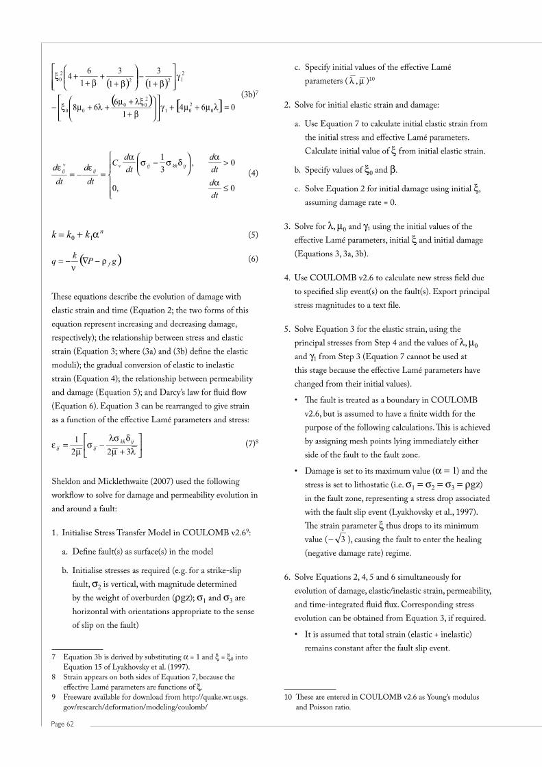
Page 62
c. Specify initial values of the effective Lamé parameters ( , )10
2. Solve for initial elastic strain and damage:
a. Use Equation 7 to calculate initial elastic strain from the initial stress and effective Lamé parameters. Calculate initial value of ξ from initial elastic strain.
b. Specify values of ξ0 and β.
c. Solve Equation 2 for initial damage using initial ξ, assuming damage rate = 0.
3. Solve for λ, µ0 and γ1 using the initial values of the effective Lamé parameters, initial ξ and initial damage (Equations 3, 3a, 3b).
4. Use COULOMB v2.6 to calculate new stress field due to specified slip event(s) on the fault(s). Export principal stress magnitudes to a text file.
5. Solve Equation 3 for the elastic strain, using the principal stresses from Step 4 and the values of λ, µ0 and γ1 from Step 3 (Equation 7 cannot be used at this stage because the effective Lamé parameters have changed from their initial values).
• ThefaultistreatedasaboundaryinCOULOMBv2.6, but is assumed to have a finite width for the purpose of the following calculations. This is achieved by assigning mesh points lying immediately either side of the fault to the fault zone.
• Damageissettoitsmaximumvalue(α = 1) and the stress is set to lithostatic (i.e. σ1 = σ2 = σ3 = ρgz) in the fault zone, representing a stress drop associated with the fault slip event (Lyakhovsky et al., 1997). The strain parameter ξ thus drops to its minimum value ( 3 ), causing the fault to enter the healing (negative damage rate) regime.
6. Solve Equations 2, 4, 5 and 6 simultaneously for evolution of damage, elastic/inelastic strain, permeability, and time-integrated fluid flux. Corresponding stress evolution can be obtained from Equation 3, if required.
• Itisassumedthattotalstrain(elastic+inelastic)remains constant after the fault slip event.
10 These are entered in COULOMB v2.6 as Young’s modulus and Poisson ratio.
0641
668
1
3
1
31
64
0201
200
00
2122
20
(3b)7
0,0
0,3
1
dt
d
dt
d
dt
dC
dt
d
dt
d ijkkijvij
vij (4)
k = k0 + k1α n (5)
gPk
q f (6)
These equations describe the evolution of damage with elastic strain and time (Equation 2; the two forms of this equation represent increasing and decreasing damage, respectively); the relationship between stress and elastic strain (Equation 3; where (3a) and (3b) define the elastic moduli); the gradual conversion of elastic to inelastic strain (Equation 4); the relationship between permeability and damage (Equation 5); and Darcy’s law for fluid flow (Equation 6). Equation 3 can be rearranged to give strain as a function of the effective Lamé parameters and stress:
3221 ijkk
ijij (7)8
Sheldon and Micklethwaite (2007) used the following workflow to solve for damage and permeability evolution in and around a fault:
1. Initialise Stress Transfer Model in COULOMB v2.69:
a. Define fault(s) as surface(s) in the model
b. Initialise stresses as required (e.g. for a strike-slip fault, σ2 is vertical, with magnitude determined by the weight of overburden (ρgz); σ1 and σ3 are horizontal with orientations appropriate to the sense of slip on the fault)
7 Equation 3b is derived by substituting α = 1 and ξ = ξ0 into Equation 15 of Lyakhovsky et al. (1997).
8 Strain appears on both sides of Equation 7, because the effective Lamé parameters are functions of ξ.
9 Freeware available for download from http://quake.wr.usgs.gov/research/deformation/modeling/coulomb/

Page 63
pmd*CRC ProjeCtS M4, M9 and F6 Final rePort
Aspects of this work were presented at the Fall meeting of the American Geophysical Union in 2007 (Sheldon and Micklethwaite, 2006), including calculation and visualisation of the damage rate in three dimensions. The COULOMB data for the 3D model is included in Appendix 2, along with a Python script for converting the COULOMB results to VTK (principal stresses, differential stress, ξ and damage rate are written to a VTK file, which can be visualised using Mayavi).
The following files are also included in Appendix 2:
• Scilabscriptsforcalculatingevolutionofdamage,strain,permeability and fluid flux, using the Hamiel et al. (2004) formulation.
• COULOMBdataforanidealisedverticalstrike-slipfault and a simplified representation of the Black Flag fault (results on a horizontal plane at 10km depth).
• Equation6issolvedfortheverticalcomponentofthe fluid flux, assuming a constant lithostatic fluid pressure gradient and zero horizontal gradient. In reality there would be a lateral component to fluid flow as fluid becomes focused through the more permeable parts of the system.
Steps 3, 5 and 6 were performed using standard Scilab11 routines to solve the differential and algebraic equations. Parameter values used by Sheldon and Micklethwaite (2007) are listed in Table 1 below.
Publications and files
Sheldon and Micklethwaite (2007) demonstrated the relationship between STM and damage mechanics using simple strike-slip fault models.
11 Freeware available for download from www.scilab.org. The following routines were used: fsolve, dassrt and dassl.
Table 1: Nomenclature and parameter values
Symbol Definition Value
C1, C2 Kinetic parameters for negative damage rate (s-1, 1)
10-5 s-1, 0.05
Cd Kinetic parameter for positive damage rate (s-1)
2.2 s-1
Cv Kinetic parameter for viscous strain rate (Pa-1)
3 x 10-11 Pa-1
g Acceleration due to gravity (ms-2)
-9.81 ms-2
I1, I2 Invariants of the elastic strain tensor: I1 = εkk, I2 = εijεij
k Permeability (m2)
k0 Permeability of undamaged rock (m2)
10-18 m2
k1 Parameter reflecting permeability enhancement due to damage (m2)
10-13 m2
n Exponent in permeability relationship
3
P Fluid pressure (Pa)
q Darcy fluid flux (m3/m2)
t Time (s)
z Vertical coordinate; positive upwards (m)
Symbol Definition Value
α Damage; represents density of cracks in representative volume of rock (0 < α < 1)
β Exponent in damage rate equation (0 < β < 1)
0.15
δij Kronecker delta; δij = 1 for i = j, δij = 0 otherwise
εijElastic strain tensor
εijv Irreversible (viscous) strain
tensor
ν Fluid viscosity (Pa s) 5 x 10⁻⁴ Pa s
λ, µ, γ Components of the effective Lamé parameters (Pa)
λ0, µ0 Lamé parameters of undamaged rock (Pa)
, Effective Lamé parameters (Pa)
100 x 109 Pa, 25 x 109 Pa
ρ, ρfDensity of solid rock and fluid (kg/m3)
2900 kg/m3, 1000 kg/m3
σijStress tensor (Pa)
ξ Strain diagonality =
21 II 33
ξ0Critical strain diagonality -0.62
Page 64
Sheldon, H.A. and Micklethwaite, M., 2006. Damage, stress transfer and mineralisation around major faults. In: Fall Meeting Supplement Eos Transactions AGU, 87(52), Abstract T23E-08.
Sheldon, H.A. and Micklethwaite, S., 2007. Damage and permeability around faults: Implications for mineralization. Geology, 35, p. 903–906.
Utsu, T., Ogata, Y. and Matsuura, R.S., 1995. The centenary of the Omori formula for a decay law of aftershock activity. Journal of Physics of the Earth, 43, p. 1–33.
2.9 Modelling Magmatic and Metamorphic Fluid Production in Flac3D
Heather A. Sheldon
Introduction
Fluids released from cooling magmas and prograde metamorphic reactions are believed to play an important role in many types of hydrothermal mineralisation (e.g. Guilbert and Park, 1986). Understanding the volumes of these fluids, their migration pathways and the timing of their release relative to tectonic/magmatic/metamorphic events is an important step in analysing hydrothermal ore systems. This paper describes a methodology for simulating magmatic and metamorphic fluid production coupled with deformation, fluid flow and heat transport. The methodology was developed in response to requirements of the pmd*CRC ’S Y4 project and was used in that project to explore aspects of fluid production relating to Archaean gold mineralisation in the Yilgarn.
Technical details
The methodology described in this paper represents the following aspects of deformation, heat transport, fluid production and fluid flow in the earth’s crust:
• Conductiveandadvectiveheattransport;
• Magmaticfluidproductiondrivenbycooling;
• Metamorphicfluidproductiondrivenbyheating;
• Latentheatofmetamorphicreactionsandmagmaticcrystallisation;
• Thermalexpansion/contractionoffluidandsolid;
References
Cox, S.F., Knackstedt, M.A. and Braun, J., 2001. Principles of structural control on permeability and fluid flow in hydrothermal systems. Reviews in Economic Geology, 14, p. 1–24.
Cox, S.F. and Ruming, K., 2004. The St Ives mesothermal gold system, Western Australia – a case of golden aftershocks? Journal of Structural Geology, 26, p. 1109–1125.
Hamiel, Y., Liu, Y., Lyakhovsky, V., Ben-Zion, Y. and Lockner, D., 2004. A visco-elastic damage model with applications to stable and unstable fracturing. Geophysical Journal International, 159, p. 1155–1165.
King, G.C.P., Stein, R.S. and Lin, J., 1994. Static stress changes and the triggering of earthquakes. Bulletin of the Seismological Society of America, 84, p. 935–953.
Lockner, D.A., 1995. Rock failure. In: Ahrens, T.J. (Ed.) Rock physics and phase relations: A handbook of physical constants. AGU reference shelf 3. American Geophysical Union, p. 127–147.
Lyakhovsky, V., Ben-Zion, Y. and Agnon, A., 1997. Distributed damage, faulting, and friction. Journal of Geophysical Research, 102, p. 27635–27649.
Main, I.G., 2000. A damage mechanics model for power-law creep and earthquake aftershock and foreshock sequences. Geophysical Journal International, 142, p. 151–161.
Micklethwaite, S. and Cox, S.F., 2004. Fault-segment rupture, aftershock-zone fluid flow, and mineralization. Geology, 32, p. 813–816.
Micklethwaite, S. and Cox, S.F., 2006. Progressive fault triggering and fluid flow in aftershock domains: Examples from mineralized Archaean fault systems. Earth and Planetary Science Letters, 250, p. 318–330.
Omori, F., 1894. On the aftershocks of earthquakes. Journal Coll. Science Imperial University of Tokyo, 7, p. 111–120.
Scholz, C.H., 1990. The mechanics of earthquakes and faulting. Cambridge University Press, Cambridge, 439 pp.
Page 65
pmd*CRC ProjeCtS M4, M9 and F6 Final rePort
by thermal expansion of the solid grains. The opposite happens during cooling. This change in pore pressure may lead to dilation, depending on the balance of forces in the surrounding rock.
Fluid production
Fluid production is represented by the apply vwell command in FLAC3D, which specifies the rate of fluid inflow into each zone (representing fluid production) with dimensions of fluid volume per unit volume of rock per unit time. The command must be applied separately to each zone in the model because each zone is subject to a different fluid production rate. This is achieved using a fish function that calculates the rate of fluid production and applies it to the relevant zone, using the command…endcommand statements to access the apply vwell command. This makes the fluid production step rather slow; it would be considerably faster if there were a FISH function equivalent to apply vwell.
For the Yilgarn models, the rate of magmatic fluid production was determined from the variation in free water content of mafic granitic magma as a function of temperature. In a closed system at 3500 bars, the mass fraction of free water (X) in the mafic granitic magma (X) is approximated by a power law:
07.0,10min 0089.821TX (2)
where T is temperature in °C ( James Cleverley, pers. comm.). This relationship can be used to calculate the rate of fluid (water) production during cooling of such a magma. The logic for each magma zone is as follows:
Store the initial mass (M0) and temperature of the zone.Calculate the initial value of X and set the porosity
consistent with this value.After each thermal step:
Calculate the change in X (due to change in T) using the power law function.
Calculate mass of water released: Mw = ∆X * M0
Rate of fluid production = Mw/(fluid density)/(zone volume)/(thermal timestep). Apply this value to the zone using the apply vwell command.
Store the new temperature of the zone.Update porosity and density to reflect the
conversion of solid (representing melt + crystals) to fluid (magmatic volatiles).
• Changesinporosityandfluidpressureduetofluidproduction, deformation and thermal expansion/contraction;
• Changesinpermeabilitylinkedtochangesinporosity;
• Deformationdrivenbychangesinfluidpressureandfar-field boundary conditions;
• Variationinfluidpropertieswithtemperatureandpressure;
• Variationinsoliddensity,thermalconductivityandspecific heat capacity with temperature.
These features were implemented using FISH12 functions in Flac3D version 3.10 (Itasca Consulting Group, 2005), a Lagrangian finite difference code which models coupled deformation, fluid flow and heat transport. Further details of the implementation are provided below.
Thermal-mechanical-fluid flow coupling
Advective and conductive heat transport is simulated in Flac3D using model th_ac. When coupled with isotropic fluid flow (model fl_iso), this thermal model13 accounts for buoyancy-driven flow (convection); that is, fluid flow driven by spatial variations in fluid density.
Deformation and fluid flow are coupled in Flac3D through the effect of volumetric strain on fluid pressure, and the influence of fluid pressure on effective stress. The pore fluid is treated as a compressible viscous fluid, governed by the fluid bulk modulus. A further degree of coupling is represented when deformation and fluid flow are combined with thermal evolution, whereby changes in temperature lead to changes in fluid pressure as the rock resists thermal expansion or contraction of the pore fluid. This “thermal pressurisation” effect is governed by the undrained thermal coefficient,β (property u_thc):
fs3 (1)
where φ is porosity, αistheBiotcoefficient(equalto1for incompressible solid grains), and βs and βf are the volumetricthermalexpansioncoefficientsofthesolidgrains and pore fluid, respectively. Fluid pressure rises with increasing temperature due to thermal expansion of the pore fluid, and due to reduction in pore space caused
12 FISH is the macro language of FLAC3D.13 Available in FLAC3D version 3.0 and above.
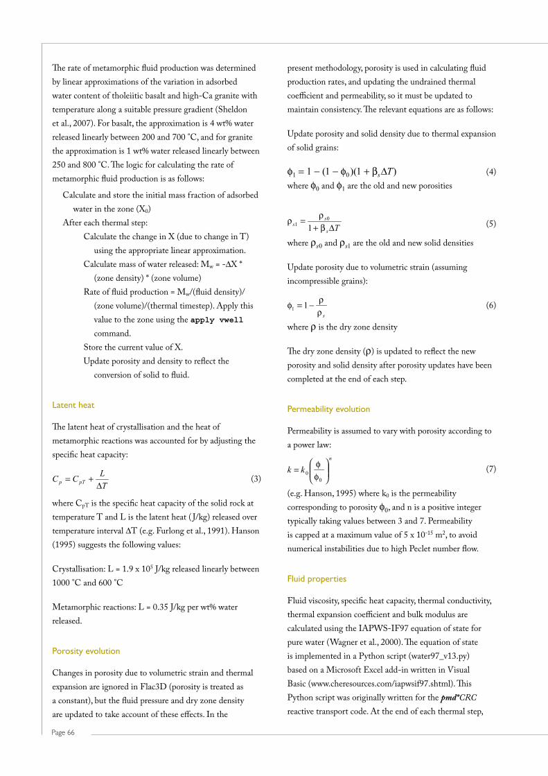
Page 66
present methodology, porosity is used in calculating fluid production rates, and updating the undrained thermal coefficientandpermeability,soitmustbeupdatedtomaintain consistency. The relevant equations are as follows:
Update porosity and solid density due to thermal expansion of solid grains:
φ1 = 1 − (1 − φ0 )(1 + βs ∆T) (4) where φ0 and φ1 are the old and new porosities
Ts
ss 1
01 (5)
where ρs0 and ρs1 are the old and new solid densities
Update porosity due to volumetric strain (assuming incompressible grains):
s
11 (6)
where ρ is the dry zone density
The dry zone density (ρ) is updated to reflect the new porosity and solid density after porosity updates have been completed at the end of each step.
Permeability evolution
Permeability is assumed to vary with porosity according to a power law:
n
kk0
0 (7)
(e.g. Hanson, 1995) where k0 is the permeability corresponding to porosity φ0, and n is a positive integer typically taking values between 3 and 7. Permeability is capped at a maximum value of 5 x 10-15 m2, to avoid numerical instabilities due to high Peclet number flow.
Fluid properties
Fluid viscosity, specific heat capacity, thermal conductivity, thermalexpansioncoefficientandbulkmodulusarecalculated using the IAPWS-IF97 equation of state for pure water (Wagner et al., 2000). The equation of state is implemented in a Python script (water97_v13.py) based on a Microsoft Excel add-in written in Visual Basic (www.cheresources.com/iapwsif97.shtml). This Python script was originally written for the pmd*CRC reactive transport code. At the end of each thermal step,
The rate of metamorphic fluid production was determined by linear approximations of the variation in adsorbed water content of tholeiitic basalt and high-Ca granite with temperature along a suitable pressure gradient (Sheldon et al., 2007). For basalt, the approximation is 4 wt% water released linearly between 200 and 700 °C, and for granite the approximation is 1 wt% water released linearly between 250 and 800 °C. The logic for calculating the rate of metamorphic fluid production is as follows:
Calculate and store the initial mass fraction of adsorbed water in the zone (X0)
After each thermal step:Calculate the change in X (due to change in T)
using the appropriate linear approximation.Calculate mass of water released: Mw = -∆X *
(zone density) * (zone volume)Rate of fluid production = Mw/(fluid density)/
(zone volume)/(thermal timestep). Apply this value to the zone using the apply vwell command.
Store the current value of X.Update porosity and density to reflect the
conversion of solid to fluid.
Latent heat
The latent heat of crystallisation and the heat of metamorphic reactions was accounted for by adjusting the specific heat capacity:
T
LCC pTp (3)
where CpT is the specific heat capacity of the solid rock at temperature T and L is the latent heat ( J/kg) released over temperature interval ∆T (e.g. Furlong et al., 1991). Hanson (1995) suggests the following values:
Crystallisation: L = 1.9 x 10⁵ J/kg released linearly between 1000 °C and 600 °C
Metamorphic reactions: L = 0.35 J/kg per wt% water released.
Porosity evolution
Changes in porosity due to volumetric strain and thermal expansion are ignored in Flac3D (porosity is treated as a constant), but the fluid pressure and dry zone density are updated to take account of these effects. In the
Page 67
pmd*CRC ProjeCtS M4, M9 and F6 Final rePort
by comparison with measured values up to 500 °C, however it produces reasonable values at higher temperatures.
Specific heat capacity increases with temperature according to a power law (Waples and Waples, 2004):
00 pnTpnTpTpT CCCC (10a)
716.01072.11013.21095.8 326310nnnnpnT TTTC (10b)
where CpT is the specific heat capacity at temperature T and CpT0 is a known value of specific heat capacity at temperature T0. This equation is valid from 0 to 1200 °C.
Applying the methodology
The algorithms described above result in many dependencies between properties in the Flac3D model so it is important that a particular sequence is followed when setting up a model. The suggested sequence is:
1. Create or import a mesh.
2. Configure the model for fluid flow and thermal calculations, and specify appropriate mechanical, thermal and fluid models.
3. Call the file “zone_functions.dat” (this file contains FISH functions implementing the algorithms described above).
4. Assign appropriate values to the mechanical properties (e.g. cohesion, friction angle), reference temperature and reference fluid density.
5. Assign initial solid densities to zextra 3.
6. Assign intrinsic permeability values to zextra 1.
7. Initialise porosity corresponding to intrinsic permeability (Equation 7).
8. Initialise temperature, fluid pressure and stress with approximate gradients (adjusted during equilibration). Magmatic intrusions should be initialised with same temperature as surrounding rock.
9. Apply fluid and thermal boundary conditions for initialisation.
716.01072.11013.21095.8 326310nnnnpnT TTTC
a FISH function writes the current values of temperature and pressure in each zone to a text file. The system command is then used to pass control to a Python script (get_water_props.py) which reads the temperature-pressure values, uses functions in water97_v13.py to calculate the corresponding water properties and writes these values to a file. Control then returns to Flac3D, where another FISH function reads the water properties from the file and uses these values to update the corresponding Flac3D properties.
The Python script returns values for fluid density, viscosity, specific heat capacity, thermal conductivity and bulk modulus. Specific heat capacity and thermal conductivity values are used to update the Flac3D properties lspec_heat and lconduct, respectively. Fluid viscosity does not appear explicitly in Flac3D; instead it is incorporated in the definition of permeability, such that kflac = k/µ (where k is intrinsic permeability in m2, and µ is fluid viscosity in Pa s). The intrinsic permeability is stored in an extra zone variable, and used in conjunction with the viscosity to update the Flac3D permeability.
The thermal advection logic in Flac3D assumes fluid density varies linearly with temperature according to a specifiedvolumetricthermalexpansioncoefficient(βf):
00 1 TTff (8)
where ρ0 is the fluid density at temperature T0 (property f_T0 in FLAC3D). This equation is used to update βf (Flac3D property f_thexp), given the current values of temperature and fluid density.
Solid properties
Several authors have published equations expressing the variation in thermal conductivity and specific heat capacity of rocks with temperature. The equations of Vosteen and Schellschmidt (2003) and Waples and Waples (2004) were chosen for the present application.
According to Vosteen and Schellschmidt (2003), the thermal conductivity of crystalline rocks decreases with increasing temperature according to the following equation:
0
0
99.0 baT (9)
where a = 0.003, b = 0.0042 and λ0 is the thermal conductivity at T = 0 °C. This equation has been validated
Page 68
(ii) Do magmatic/metamorphic fluid production; update thermal conductivity, specific heat, porosity, permeability, dry density, undrained thermal coefficient,andfluidproperties;
(iii) Take N fluid + deformation steps (thermal off, flow on, mechanical on), where N is determined by size of fluid flow step relative to thermal step;
(iv) Update volumetric strain, porosity and permeability.
Publications and appendices
The methodology described above was used in the pmd*CRC Y4 project to address questions regarding the volume, timing and relative significance of magmatic and metamorphic fluid production in the Yilgarn. More details can be found in the final report of the Y4 project (Blewett, 2008; specifically Deliverable 11 and Section III).
FISH functions implementing the equations outlined above can be found in the files zone_functions.dat, magmatic_fluids.fis and metamorphic_fluids.fis. These files are contained in a zip archive in Appendix 2 (mag_met_fluids_Flac3D.zip), along with the Python script and associated FISH functions implementing the IAPWS-IF97 equation of state for water. Also included is an example of a Flac3D data file to run a model including magmatic/metamorphic fluid production.
References
Blewett, R.S. (Ed.), 2008. Concepts to targets: A scale integrated mineral systems study of the eastern Yilgarn craton. (in prep.)
Furlong, K.P., Hanson, R.B. and Bowers, J.R., 1991. Modeling thermal regimes. Reviews in Mineralogy, 26, p. 437–505.
Guilbert, J.M. and Park, C.F., 1986. The geology of ore deposits. Freeman, New York.
Hanson, R.B., 1995. The hydrodynamics of contact-metamorphism. Geological Society of America Bulletin, 107, p. 595–611.
Itasca Consulting Group, 2005. Flac3D: Fast lagrangian analysis of continua in 3 dimensions. Itasca, Minneapolis.
10. Initialise fluid properties using the IAPWS-IF97 routines.
11. Initialise thermal conductivity and specific heat capacity of solid (Equations 9 and 10).
12. Initialise dry zone density in accordance with solid density and porosity.
13. Equilibrate:
(i) Thermal only, with permeability set to zero (to establish conductive geotherm); update temperature-dependent properties periodically during thermal equilibration;
(ii) Fluid flow only, with permeability set to an arbitrary constant value throughout model;
(iii) Deformation + fluid flow, with permeability set to true value (based on intrinsic permeability and fluid viscosity).
14. Reset velocities and displacements to zero. Reset thermal and fluid time to zero.
15. Initialise velocities for far-field deformation (if required).
16. Store initial zone volumes for calculation of volumetric strain.
17. Set up metamorphic fluid production: Assign flags to each zone undergoing metamorphic fluid production; Calculate and store initial mass fraction of adsorbed water for each zone.
18. Initialise temperature in magmatic intrusions.
19. Store initial temperature and update undrained thermalcoefficient(Equation1).
20. Setup magmatic fluid production: Assign a flag to each zone undergoing magmatic fluid production; Calculate and store initial zone mass, and initialise porosity in magma zones according to mass fraction of free water.
21. Setup histories and particle tracking (if required).
22. Run the model, repeating the following sequence in a loop until desired time is reached:
(i) Take 1 thermal step (thermal on, flow off, mechanical off );

Page 69
pmd*CRC ProjeCtS M4, M9 and F6 Final rePort
understand factors controlling free convection in geological systems in order to understand the significance of this process for mineralisation.
Conditions for the onset of free convection (e.g. minimum permeability) can be determined exactly for simple systems, such as an infinite horizontal layer with constant properties and boundary conditions. Natural systems are characterised by complex geometries and highly variable properties so numerical models are needed to understand free convection in specific geological systems.
This paper reviews some results from both types of analysis and considers implications for the occurrence of free convection in the Earth’s crust. Systems containing local sources of heat or salt (e.g. intrusions) are excluded because the horizontal density gradients in such systems will always result in convection (Phillips, 1991). The focus here is on free convection in areas characterised by uniform, approximately vertical gradients in temperature and salinity. Much of the information is drawn from Phillips (1991) and Nield and Bejan (1992), with additional material from more recent publications.
Conditions for free convection
In qualitative terms, free convection can take place if the buoyancy force associated with a density gradient (e.g.duetoincreasingtemperaturewithdepth)issufficientto overcome viscous resistance to flow, and if the resulting flow transports heat or solute faster than it is dissipated by diffusion. A technique known as linear stability analysis can be used to quantify the conditions under which free convection can take place in simple systems, by examining the behaviour of the non-convective steady state (e.g. a uniform vertical temperature gradient) in response to a small perturbation. For the purpose of such analysis, it is common practice to simplify the governing equations by making the Boussinesq approximation. This means all properties of the porous medium and pore fluid are assumed to be constant except the fluid density where it appears in the buoyancy term of the momentum equation. There, the fluid density is assumed to vary linearly with temperature and/or salinity.
Free thermal convection
We begin by considering the conditions for free thermal convection; that is, free convection in a system in which the
Sheldon, H.A., Barnicoat, A.C., Zhang, Y. and Ord, A., 2007. Metamorphism in the eastern goldfields: Implications for fluid flow and mineralisation. In: Bierlein, F.P. and Knox-Robinson, C.M. (Eds.), Proceedings of Geoconferences (WA) Inc. Kalgoorlie ‘07 Conference, Geoscience Australia Record 2007/14. Geoscience Australia, Canberra, Australia, p. 138–142.
Vosteen, H.D. and Schellschmidt, R., 2003. Influence of temperature on thermal conductivity, thermal capacity and thermal diffusivity for different types of rock. Physics and Chemistry of the Earth, 28, p. 499–509.
Wagner, W. et al., 2000. The IAPWS industrial formulation 1997 for the thermodynamic properties of water and steam. Journal of Engineering for Gas Turbines and Power-Transactions of the ASME, 122, p. 150–182.
Waples, D.W. and Waples, J.S., 2004. A review and evaluation of specific heat capacities of rocks, minerals, and subsurface fluids. Part 1: Minerals and nonporous rocks. Natural Resources Research, 13, p. 97–122.
2.10 Conditions for Free Convection in the Earth’s Crust
Heather A. Sheldon
Introduction
Fluid flow in the Earth’s crust is driven by the combined effects of topography, deformation, chemical reactions and buoyancy. Flow driven by buoyancy alone is described as free convection, which occurs due to unstable gradients in fluid density associated with variations in temperature and fluid composition (especially salinity) (Cheng, 1985; Nield and Bejan, 1992; Phillips, 1991). Free convective flow is characterised by convection cells that connect upwelling and downwelling regions. This flow pattern could play an important role in hydrothermal mineralisation for a number of reasons (Zhao et al., 2004): (i) circulation of fluid in a closed system could account for the large time-integrated fluid fluxes that are needed to explain observed mineralisation in some hydrothermal systems; (ii) convective circulation may facilitate fluid mixing; (iii) convective flow transports solutes through temperature gradients and gradients in solubility; and (iv) it could explain the regular spacing of hydrothermal deposits along some faults (Ord, pers. comm.). It is important to

Page 70
Rac changes if the lower and upper boundary conditions are modified (Nield and Bejan, 1992). For example, Rac = 17.65 for the case of an infinite horizontal layer with a fixed heat flux and impermeable boundary at the base, and with fixed temperature and fixed fluid pressure at the top. This could represent a layer of rock or sediment with the upper boundary at the earth’s surface and the lower boundary resting on relatively impermeable basement rocks. Rac is reduced further to 12 if both boundaries are impermeable and subject to constant heat flux, representing a permeable unit sealed above and below by less permeable horizons.
Fault zones may be regarded as narrow, permeable boxes embedded in less permeable rocks. The analysis of Beck (1972) suggests Rac would be close to 4π2 for the case of a fault with fixed temperature, impermeable boundaries at the top and base, and impermeable, perfectly insulated side walls. In reality, fault zones are not completely isolated from surrounding rocks; there is always some exchange of heat and fluid between the fault and its host rocks so the assumption of impermeable, perfectly insulated sidewalls is inappropriate. Zhao et al. (2003) considered the case of a 3D box with length > height > width, with the temperature being fixed at the geothermal gradient and fluid pressure fixed at hydrostatic on the long sidewalls. This scenario approximates a vertical fault zone embedded in conductive, slightly permeable wallrocks. Zhao et al. (2003) showed the critical Rayleigh number in this system increases with the ratio of height to width, so a tall, narrow fault zone may have Rac >> 4π2 (Figure 45). In reality the situation would be somewhere between the perfectly conductive case
fluid density depends only on temperature. Linear stability analysis shows that free thermal convection takes place if the Rayleigh number (RaT) exceeds a critical value (Rac). For the case of a horizontal layer with temperature T1 at the lower boundary and T0 at the upper boundary, RaT is defined as:
TckgHRa p
T
20 (1a)
where g is gravity (m/s2), H is the height of the system (m), k is permeability (m2), ∆T = T1 – T0 (°K), cp is the specific heat capacity of the pore fluid ( J/kg/°K), α is the volumetricthermalexpansioncoefficientoftheporefluid(1/°K), µ is fluid viscosity (Pa s), and λ is the thermal conductivity of the fluid-saturated porous medium (W/m/°K). Alternatively, the Rayleigh number can be expressed in terms of the conductive heat flux q associated with a given thermal gradient, q = −λ ∂T /∂z (z increasing upwards):
qckgHRa p
T
20
2
(1b)
For the case of an infinite horizontal layer of height H, subject to fixed temperature and impermeable boundaries at the top and base, and starting with a uniform thermal gradient and hydrostatic fluid pressure, the value of Rac is 4π2 (Horton and Rogers, 1945; Lapwood, 1948). Beck (1972) showed that Rac remains close to 4π2 in a 3D box of finite length and width with impermeable boundaries all round, fixed temperature at the top and base, and perfectly insulated sidewalls, as long as the height is smaller than the width or length. Higher values of Rac are obtained if both the width and length are less than height.
Figure 45: Rac for 3 convection modes in a permeable fault zone as a function of
fault height and width. (Zhao et al. 2003.)

Page 71
pmd*CRC ProjeCtS M4, M9 and F6 Final rePort
Equation 3 implies an increase in salinity with depth always stabilises the system relative to the purely thermal case. For example, an increase in salinity of just 0.51 kg/m3 (i.e.~0.00051wt%)overadepthof10kmissufficientto reduce Ra to zero, assuming a geothermal gradient of 30°/km, φ = 1% and β = 0.001 m3/kg. Conversely, a decrease in salinity with depth by the same amount would double the Rayleigh number. However, it is important to note equation 3 was obtained by linear stability analysis of a system characterised by initially uniform gradients of temperature and salinity. Numerical models presented by Schoofs et al. (1999) and Geiger et al. (2005) indicate the effect of salinity may differ if the initial condition represents a step-increase in salinity and temperature at the base, rather than a smooth gradient from top to base. Their models predict free convection in cases where Equation 3 suggests it should not be possible. In the numerical models, heat and solute diffuse upward from the lower boundary, but heat diffuses faster than salinity so the system becomes thermally unstable, triggering free convection. Subsequent behaviour is influenced by salinity as the solute becomes entrained in the thermally-driven flow. Schoofs et al. (1999) showed that the behaviour becomes increasingly chaotic with increasing salinity for models with low porosity (1%). The sources of heat and salinity must be taken into account when determining whether free convection can occur in a given geological system.
Effect of throughflow on free convection
Horizontal throughflow may be considered a proxy for topographically-driven flow (e.g. Raffensperger and Vlassopoulos, 1999). Rac is unchanged by imposing a uniform horizontal fluid velocity on a horizontal layer; the only difference is that free convection occurs in a coordinate system moving at the speed of the horizontal throughflow (Nield and Bejan, 1992). The convection cells migrate along the layer, reducing the potential for localised alteration or mineralisation that could occur if they were stationary (Raffensperger and Vlassopoulos, 1999). However, horizontal throughflow tends to inhibit convection even though it does not affect Rac, because dispersion increases with fluid velocity. Effectively this means Ra decreases with the rate of horizontal throughflow and may eventually drop below the critical value.
Upward throughflow could represent several geological processes, such as a regional upward fluid flux associated
considered by Zhao et al. (2003) and the perfectly insulated case considered by Beck (1972). Numerical models are needed to determine the critical Rayleigh number in the case where the sidewalls are neither perfectly conducting nor perfectly insulating.
Zhao et al. (2004) explored the effect of fault dip on Rac, using the same boundary conditions as Zhao et al. (2003). They showed Rac decreases with decreasing dip for a given vertical height of the inclined box. Thus, for a dipping fault cutting through a horizontal layer of a given thickness, the critical Rayleigh number decreases with decreasing dip angle.
Free thermohaline convection
The term thermohaline refers to free convection driven by the combined effects of heat and salt on fluid density. Unlike heat, salt cannot diffuse through the solid matrix. This means that heat is advected more slowly and diffuses more rapidly than salt (Phillips, 1991; Schoofs et al., 1999). The terms “double diffusive” and “double advective” are used to emphasise the difference in transport rates. Consequently, the effect of a salinity gradient on free convection cannot be inferred from its effect on density alone.
For a system in which the fluid density depends linearly on both salinity and temperature, the Rayleigh number is modified by a factor reflecting the effect of salinity on fluid density and the different transport rates of heat and solute (Phillips, 1991):
T
SRaRa T 1 (3)
where α and βarethevolumetricexpansioncoefficientsof the pore fluid with respect to temperature and salinity; φ is porosity; ∆S and ∆T are the changes in temperature and salinity between the upper and lower boundaries; and Γ = (ρcp )s /(ρcp )f reflects the relative heat-carrying capacity of fluid and solid. Equation 3 is valid if the solute diffusivity (φD) is smaller than the thermal diffusivity (κ), which is likely in low porosity rocks, although mechanical dispersion of solute might influence the behaviour somewhat (Schoofs et al., 1999). Equation 3 differs from the result obtained by Nield (1968), who considered double diffusive effects but did not account for the difference in advection rates between heat and solute (Phillips, 1991).

Page 72
(and salinity). In reality, fluid properties such as viscosity and thermal expansion vary by orders of magnitude within the earth’s crust, and their variation is highly non-linear with respect to pressure, temperature and composition.
Lin et al. (2003) used linear stability analysis to show an exponential decrease in fluid viscosity with increasing temperature results in a decrease in Rac relative to the constant viscosity case. Unfortunately the exponential function used by Lin et al. (2003) is not a particularly good representation of the variation of pore fluid viscosity with temperature in natural systems. Numerical methods must be used to determine the impact of more realistic variations in fluid properties. Straus and Schubert (1977) used numerical models to explore the significance of non-Boussinesq effects in uniform horizontal layers up to 10km thick, in which the fluid properties were calculated from an equation-of-state for pure water. Their results showed the critical Rayleigh number could be reduced by as much as a factor of 31 relative to the value for a Boussinesq fluid, largely due to the variation in fluid viscosityandthermalexpansioncoefficientbetweenthetop and base of the layer. However, Straus and Schubert (1977) noted these effects might be counteracted in natural systems by the tendency for permeability to decrease with depth.
Boiling and phase separation introduce an additional level of complexity in high temperature, low pressure systems. Modelling such behaviour is a challenge but recent work by Geiger et al. (Driesner and Heinrich, 2003; Geiger et al., 2005, 2006a, b) has addressed some of the issues.
with metamorphism, or compaction-driven flow in sediments. Intuitively one might expect upward throughflow would inhibit free convection. Linear stability analysis confirms this expectation (i.e. Rac increases with the rate of upward flow) for the case of a horizontal layer with fixed T at the top and base, a fixed fluid flux at the base, and fixed fluid pressure at the top (Cheng, 1985; Nield and Bejan, 1992; and references therein). More recently it has been shown that Rac actually decreases with increasing upward throughflow if the lower boundary of the system is subject to a fixed thermal gradient rather than fixed temperature (Zhao et al., 1999). This means free thermal convection may be possible in overpressured regions of the crust, depending on the boundary conditions of the system. However, caution is needed in applying these results to natural systems because the analysis assumes the system starts from the non-convective steady state for the specified boundary conditions. This steady state is geologically unrealistic for moderate degrees of fluid overpressure (Figure 46; note extreme thermal gradient near surface), and may never be attained in a natural system in which the fluid flux exists for only a finite time period. Thus, numerical models are required to determine the effect of upward throughflow in specific geological scenarios.
Effect of variable fluid properties (non-Boussinesq effects)
Most analyses of free convection are based on the Boussinesq approximation, where properties of the fluid and solid are assumed to be constant, except the fluid density which is assumed to vary linearly with temperature
Figure 46: Non-convective steady-state temperature in a horizontal layer with upward
throughflow and fixed thermal gradient at the base. Rate of throughflow determined by
degree of overpressure (0 = hydrostatic, 1 = lithostatic), assuming k = 10-18 m2.

Page 73
pmd*CRC ProjeCtS M4, M9 and F6 Final rePort
suggests that, in the absence of a salinity gradient, free convection is only possible in areas of anomalously high permeability. Fault zones could satisfy this requirement, although the analysis of Zhao et al. (2003) suggests Rac could be much larger in narrow fault zones (see Figure 45), potentially offsetting the effect of higher permeability. Porous sedimentary rocks, such as sandstones, may have sufficientlyhighpermeabilitytopermitconvection(e.g.athicknessof~300–400missufficientforfreeconvectionat a typical sandstone permeability of 10-12 m2), but the presence of thin, low permeability layers could reduce the effective permeability below the critical value (Bjorlykke et al., 1988).
Comparing Figure 47D with Figures 47A, B and C illustrates the impact of variation in fluid properties with T and P. The permeability needed for free convection is reduced by more than 1 order of magnitude when varying fluid properties are taken into account. The permeability values in Figure 47D were calculated using fluid properties at the mid point of the horizontal layer, so are only estimates. Numerical models are needed to determine the exact permeability for free convection in a system with variable fluid properties.
A numerical model was constructed in the RT utility to explore the onset of free convection in a horizontal layer with varying permeability and fluid properties. Permeability varies with depth according to the curve of Shmonov et al. (2003) multiplied by a constant factor N. Fluid properties are determined by the IAPWS equation of state for pure
They developed a self-consistent equation-of-state for the water-halite system over the range 0 to 750 degrees C, 0 to 4000 bar, and 0–100 wt.% NaCl, and implemented it in a numerical model that accounts for boiling, phase separation and two phase flow. Their numerical results suggest free convection is inevitable if a vapour phase exists anywhere in the system, which is likely in magmatic systems such as porphyry and epithermal environments.
Minimum permeability for free convection
In this section we use results discussed above to calculate the minimum permeability needed for free convection under a range of conditions, and consider the results in the light of typical crustal permeabilities.
Figure 47 shows the minimum permeability for free convection in a horizontal layer as a function of H, geothermal gradient, Rac and ∆S. Also shown are two estimates of “average” crustal permeability. Shmonov et al. (2003) derived their permeability-depth curve from laboratory measurements of permeability, whereas Manning and Ingebritsen (1999) collated permeability estimates based on borehole measurements and the progress of metamorphic reactions. The difference between the curves (about 1–2 orders of magnitude) is consistent with the scale-dependence of permeability (e.g. Clauser, 1992). It isobviousthese“average”permeabilitiesareinsufficienttoallow free convection at reasonable geothermal gradients (Figures 47A to D), unless the system is destabilised by a decrease in salinity with depth (Figure 47E). This
Figure 47: Minimum permeability
(k) required for free convection in a
horizontal layer of varying thickness,
and average crustal permeability
curves of Shmonov et al. (2003)
and Manning and Ingebritsen
(1999). A, B and C show effect of
varying geothermal gradient and Rac
(assuming constant fluid properties:
µ = 5 x 10⁻⁴ Pa s; cp = 4180 kg/m3;
α = 10-4 °K-1). (D) Fluid properties
determined by IAPWS equation of
state for pure water at mid point of
layer. (E) Effect of decreasing salinity
with depth (Rac = 17.65).
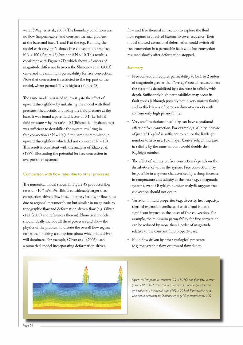
Page 74
flow and free thermal convection to explore the fluid flow regime in a faulted basement-cover sequence. Their model showed extensional deformation could switch off free convection in a permeable fault zone but convection resumed shortly after deformation stopped.
Summary
• Freeconvectionrequirespermeabilitytobe1to2ordersof magnitude greater than “average” crustal values, unless the system is destabilised by a decrease in salinity with depth.Sufficientlyhighpermeabilitiesmayoccurinfault zones (although possibly not in very narrow faults) and in thick layers of porous sedimentary rocks with continuously high permeability.
• Verysmallvariationsinsalinitycanhaveaprofoundeffect on free convection. For example, a salinity increase of just 0.51 kg/m3issufficienttoreducetheRayleighnumber to zero in a 10km layer. Conversely, an increase in salinity by the same amount would double the Rayleigh number.
• Theeffectofsalinityonfreeconvectiondependsonthedistribution of salt in the system. Free convection may be possible in a system characterised by a sharp increase in temperature and salinity at the base (e.g. a magmatic system), even if Rayleigh number analysis suggests free convection should not occur.
• Variationinfluidproperties(e.g.viscosity,heatcapacity,thermalexpansioncoefficient)withTandPhasasignificant impact on the onset of free convection. For example, the minimum permeability for free convection can be reduced by more than 1 order of magnitude relative to the constant fluid property case.
• Fluidflowdrivenbyothergeologicalprocesses(e.g. topographic flow, or upward flow due to
water (Wagner et al., 2000). The boundary conditions are no flow (impermeable) and constant thermal gradient at the base, and fixed T and P at the top. Running the model with varying N shows free convection takes place if N = 100 (Figure 48), but not if N ≤ 10. This result is consistent with Figure 47D, which shows ~2 orders of magnitude difference between the Shmonov et al. (2003) curve and the minimum permeability for free convection. Note that convection is restricted to the top part of the model, where permeability is highest (Figure 48).
The same model was used to investigate the effect of upward throughflow, by initialising the model with fluid pressure > hydrostatic and fixing the fluid pressure at the base. It was found a pore fluid factor of 0.1 (i.e. initial fluid pressure = hydrostatic + 0.1(lithostatic – hydrostatic)) wassufficienttodestabilisethesystem,resultinginfree convection at N = 10 (c.f. the same system without upward throughflow, which did not convect at N = 10). This result is consistent with the analysis of Zhao et al. (1999), illustrating the potential for free convection in overpressured systems.
Comparison with flow rates due to other processes
The numerical model shown in Figure 48 produced flow rates of ~10-9 m3/m2/s. This is considerably larger than compaction-driven flow in sedimentary basins, or flow rates due to regional metamorphism but similar in magnitude to topographic flow and deformation-driven flow (e.g. Oliver et al. (2006) and references therein). Numerical models should ideally include all these processes and allow the physics of the problem to dictate the overall flow regime, rather than making assumptions about which fluid driver will dominate. For example, Oliver et al. (2006) used a numerical model incorporating deformation-driven
Figure 48: Temperature contours (25–475 °C) and fluid flow vectors
(max. 2.86 x 10⁻⁹ m3/m2/s) in a numerical model of free thermal
convection in a horizontal layer (100 x 30 km). Permeability varies
with depth according to Shmonov et al. (2003) multiplied by 100.

Page 75
pmd*CRC ProjeCtS M4, M9 and F6 Final rePort
Geiger, S., Driesner, T., Heinrich, C.A. and Matthäi, S.K., 2006b. Multiphase thermohaline convection in the Earth’s crust: II. Benchmarking and application of a finite element – finite volume solution technique with a NaCl-H2O equation of state. Transport in Porous Media, 63, p. 435–461.
Horton, C.W. and Rogers, F.T., 1945. Convection currents in a porous medium. Journal of Applied Physics, 16, p. 367–370.
Lapwood, E.R., 1948. Convection of a fluid in a porous medium. Proceedings of the Cambridge Philosophical Society, 44, p. 508–521.
Lin, G., Zhao, C.B., Hobbs, B.E., Ord, A. and Muhlhaus, H.B., 2003. Theoretical and numerical analyses of convective instability in porous media with temperature-dependent viscosity. Communications in Numerical Methods in Engineering, 19, p. 787–799.
Manning, C.E. and Ingebritsen, S.E., 1999. Permeability of the continental crust: Implications of geothermal data and metamorphic systems. Reviews of Geophysics, 37, p. 127–150.
Nield, D.A., 1968. Onset of thermohaline convection in a porous medium. Water Resources Research, 11, p. 553–560.
Nield, D.A. and Bejan, A., 1992. Convection in porous media. Springer-Verlag, New York.
Oliver, N.H.S. et al., 2006. Numerical models of extensional deformation, heat transfer, and fluid flow across basement-cover interfaces during basin-related mineralization. Economic Geology, 101, p. 1–31.
Phillips, O.M., 1991. Flow and reactions in permeable rocks. Cambridge University Press, Cambridge, UK, 285p. pp.
Raffensperger, J.P. and Vlassopoulos, D., 1999. The potential for free and mixed convection in sedimentary basins. Hydrogeology Journal, 7, p. 505–520.
Schoofs, S., Spera, F.J. and Hansen, U., 1999. Chaotic thermohaline convection in low-porosity hydrothermal systems. Earth and Planetary Science Letters, 174, p. 213–229.
metamorphic dehydration) does not necessarily inhibit or override convection. In some cases it may actually promote convection (by reducing Rac). Importantly, free convection may be possible in overpressured systems. Convective flow rates are comparable with rates of topographic flow and deformation-driven flow.
• Linearstabilityanalysisprovidesinsightintotheconditions that are required for free convection in simple systems, but cannot deal with the complex geometries and variable properties of natural systems. Furthermore, the analysis assumes that the system starts from a steady state, which may be unrealistic.
• Numericalmodelsarerequiredtoexplorefreeconvection in natural systems with complex geometries, variable properties and boundary conditions, and competing fluid driving forces.
References
Beck, J.L., 1972. Convection in a box of porous material saturated with fluid. Physics of Fluids, 15, p. 1377–1383.
Bjorlykke, K., Mo, A. and Palm, E., 1988. Modelling of thermal convection in sedimentary basins and its relevance to diagenetic reactions. Marine and Petroleum Geology, 5, p. 338–351.
Cheng, P., 1985. Geothermal heat transfer. In: Rohsenow, W.M. (Ed.) Handbook of heat transfer applications. McGraw Hill, New York, p. 11.1–11.54.
Clauser, C., 1992. Permeability of crystalline rocks. EOS, 73, p. 231–237.
Driesner, T. and Heinrich, C.A., 2003. Accurate P-T-X-V-H correlations for the system NaCl-H2O from 0 to 800 °C, 0 to 500 MPa, and 0 to 1 X(NaCl). In: ECROFI 2003 Proceedings, Mineralogica-Petrographica Abstract Series 2, Budapest, p. 55–56.
Geiger, S., Driesner, T., Heinrich, C.A. and Matthäi, S.K., 2005. On the dynamics of NaCl-H2O fluid convection in the Earth’s crust. Journal of Geophysical Research, 110, p.
Geiger, S., Driesner, T., Heinrich, C.A. and Matthäi, S.K., 2006a. Multiphase thermohaline convection in the earth’s crust: I. A new finite element – finite volume solution technique combined with a new equation of state for NaCl-H2O. Transport in Porous Media, 63, p. 399–434.

Page 76
An opportunity therefore exists in the development and application of particle codes (a subset of the “meshless” group of codes). In a particle code, the material modelled is represented by a series of discs (in 2D) or balls (in 3D). Newton’s Laws of Motion plus simple elastic, viscous and frictional contact laws govern the motion of these particles, such that realistic behaviours emerge spontaneously without the need for empirical constitutive laws. pmd*CRC researchers and interns have used the particle code PFC (Itasca, 2004) to explore various aspects of rock deformation. Some outcomes are summarised below.
Shear localisation and permeability evolution
In contrast to continuum modelling codes where localisation or shear banding arises through a bifurcation in a predefined system of differential equations (e.g. the Mohr Coulomb constitutive model), shear bands emerge in particle simulations with no prescribed mathematical relations other than simple contact relationships between particles. Shear bands emerge from the self-organisation of large numbers of particles with long-range geometrical interactions playing a dominant role; both translation and rotation of particles are important. Initially, on loading, instabilities develop then decay into stable configurations of particles but with continued loading, force chains collapse locally to generate geometrically necessary fractures. These zones then propagate to generate localisation zones. When these fractures form a continuous network, the system is at the percolation threshhold for broken bonds (Ord et al. 2007; Zhang and Ord 2008).
Such numerical experiments may be used to improve understanding of the evolution of porosity and permeability during deformation. The pmd*CRC has explored two ways of quantifying permeability evolution: (1) Estimating permeability from porosity using the Kozeny-Carman relationship; (2) Measuring permeability directly by modelling the flow of fluid through the pore spaces between particles. The results indicate an order of magnitude increase in permeability associated with shear band development. Important for porosity development, localisation in granular media is more complicated than in continua because the motion of one grain is strongly influenced by grains many times removed from it and the development of a through-going localised band is the result of long histories of damage accumulation.
Shmonov, V.M., Vitiovtova, V.M., Zharikov, A.V. and Grafchikov, A.A., 2003. Permeability of the Continental Crust: Implications of Experimental Data. Journal of Geochemical Exploration, 78–9, p. 697–699.
Straus, J.M. and Schubert, G., 1977. Thermal convection of water in a porous medium: Effects of temperature- and pressure-dependent thermodynamic and transport properties. Journal of Geophysical Research, 82, p. 325–333.
Wagner, W. et al., 2000. The IAPWS industrial formulation 1997 for the thermodynamic properties of water and steam. Journal of Engineering for Gas Turbines and Power – Transactions of the ASME, 122, p. 150–182.
Zhao, C.B., Hobbs, B.E. and Muhlhaus, H.B., 1999. Theoretical and numerical analyses of convective instability in porous media with upward throughflow. International Journal for Numerical and Analytical Methods in Geomechanics, 23, p. 629–646.
Zhao, C.B., Hobbs, B.E., Muhlhaus, H.B., Ord, A. and Lin, G., 2003. Convective instability of 3-d fluid-saturated geological fault zones heated from below. Geophysical Journal International, 155, p. 213–220.
Zhao, C.B. et al., 2004. Theoretical investigation of convective instability in inclined and fluid-saturated three-dimensional fault zones. Tectonophysics, 387, p. 47–64.
2.11 Modelling Deformation with Particle Codes
Alison Ord
Introduction
Folding, fracturing and brecciation are fundamental geological processes, which are critical to our understanding of mineralising systems. We already have tools that enable us to model many geological processes. However, realistic simulation of folding, fracturing and brecciation processes requires the ability to proceed to very high strains; the ability to represent new fracture systems which are able to propagate as fluid or magma filled cracks; and the ability to evolve into geologically realistic geometries (e.g. folds) without prior “seeding” of the model with imperfections. All these aspects are hard to achieve or appear unnatural with continuum codes such as Flac3D (Itasca, 2002).

Page 77
pmd*CRC ProjeCtS M4, M9 and F6 Final rePort
Fluid-driven deformation: Veins and breccias
Mikula et al. (2007) used the fluid-mechanical coupling
functionality in PFC to explore fluid-driven deformation
processes, with the aim of understanding the formation of
hydrothermal veins and breccias. The goal was to describe
not just the processes critical to the formation of veins
and breccias, but the ranges of material behaviours and
boundary conditions which favour the formation of one
or the other. An approach used in research on multiphase
flow was used to develop flow regime maps of bulk rock
strength versus fluid velocity versus porosity for rock
masses invaded by fluids. Preparation of flow regime maps
is fundamental to the interpretation of breccia textures in
the field because a particular texture within a rock strength/
fluid velocity/porosity field can be positioned on the map.
The geological applications are considerable; development
of this area would benefit mineral formation predictions
and understanding of fracture formation.
Figures 49 and 50 illustrate two types of fluid-driven
deformation behaviour. In both an isolated pulse of
overpressured fluid was applied to the base of a particle
model. This results in different behaviours, depending on
the rheology of the fluid. A high viscosity fluid acts as an
intrusive dyke (Figure 49), resulting in microfracturing and
jointing through the host rock. The evolving microfractures
develop permeable pathways for volatile escape from
the intrusion. A low viscosity fluid (Figure 50) produces
fracturing ahead of the migrating pulse with subsequent
collapse of the fractured rock into the space left in the
wake of the pulse. This simulates brecciation as fluid-driven
(hydraulic) fracturing, followed by fluidisation of the
resulting fragments. Figure 51 shows the effects of varying
fluid flow rate and particle bond strength on the behaviour.
Understanding damage evolution during deformation
Laboratory experiments and observations of naturally
deformed rocks indicate the macroscopic mode by which a
rock fails depends on the effective pressure – the difference
between the confining pressure applied to the rock and
the pore fluid pressure within it. At low effective pressure
strain-softening is observed after the peak stress and a
loaded rock will fail, by shear localisation, in a brittle
fashion. In contrast, at high confinement, strain-hardening
leads to delocalised flow behaviour. This illustrates that
rheology does not depend on crack density alone but also
on how the cracks are organised.
To understand the effects of this organisation, we need
to have reliable information about the location, geometry
and orientations of these cracks, the type of motion
associated with them and the evolution of these properties
with loading. During deformation of rock in mining and
laboratory situations, Acoustic Emissions (AE), associated
with microcracking and compaction can be recorded
and provide an indication of the inelastic strain involved.
However, this strain is not accommodated uniformly
within the rock and has been associated with a range of
different mechanisms. Source analysis of AE, for example
by moment tensor inversion, can provide information
about the nature and orientation of these sources and
their evolution during loading. Source mechanisms from
inversion of AE data may be compared to modelled crack
interaction scenarios. The process of damage progression
and the onset of localisation may be explored using forward
modelling, to provide a controlled set of computational
experiments for comparison with inverted data. The aim is
to investigate the interaction of fracture mechanisms and
its importance to the onset of failure.
Figure 49: Magmatic material (brown) intrudes
through a layered sequence of granite (blue)
and sandstone (yellow) under a lithostatic
stress regime. The sandstone is damaged
pervasively (possibly observable as fluidised
clastics; pale green and pink cracks) while the
granite is broken in only a few areas (J. Malcolm,
pmd*CRC intern).

Page 78
Acknowledgments
Work reported here draws on contributions from several pmd*CRC researchers and interns, including Yanhua Zhang (CSIRO), Fabio Boschetti (CSIRO), Sarah Mikula (UWA), Caroline Graham (University of Edinburgh), Jo Malcom (University of Alaska Fairbanks) and Abhishek Srivastava (Indian Institute of Technology, Kanpur). Interns were funded by iVEC and the pmd*CRC.
Future developments
The geological community has been using particle codes increasingly over the past decade. This uptake is expected to accelerate as rock mechanics and computational simulation are further integrated into the way geologists work. The developments above will help address deep crustal to shallow mantle issues, such as melt transport, emplacement of plutons and development of fluid pathways.
Figure 51: Effect of varying bond strength and flow rate on the behaviour of the system
with cohesive sidewalls. (Mikula et al., 2007)
Figure 50: Fluids introduced along the base of a virtual rock mass result in fracturing
(small black lines) and uplift of the central section (as a result of the central free surface).
Grey bands indicate layers of cohesionless particles. (Mikula et al., 2007)
Page 79
pmd*CRC ProjeCtS M4, M9 and F6 Final rePort
commercial chemical solver WinGibbs derived from the HCh modelling code (Shvarov and Bastrakov, 1999). The RT code is run through the Desktop Modelling Toolkit (DMT). Technical descriptions of these codes and the mathematics behind them can be found elsewhere in this report. The code and its application has also been discussed in various publications, including Cleverley and Bastrakov (2005); Cleverley et al. (2006); and Cleverley (2007).
The Grid
A key goal of the pmd*CRC has been delivery of the capability to run simulations via the grid, which allows access to supercomputing facilities throughout Australia. This has required close collaboration with the AcCesS MNRF and Auscope projects to build the infrastructure that the DMT needed to utilise supercomputing facilities. At the end of the pmd*CRC we have the ability to run fluid flow-thermal models via the grid, however reactive transport models still require a Windows platform (due to the third-party chemical solver) and cannot be run on the linux-based grid systems.
Workflow
The workflow for DMT-RT modelling is broadly as follows:
• Developaconceptualmodel;
• Builditsgeometryinamodellingandmeshingpackage– for 2D models this can often be achieved in GMSH (www.geuz.org/gmsh/);
• GenerateanumericalmeshandconverttoanXML4FEM file through the DMT;
• ImportthegeometryintoDMTandallocatetheregions;
• DefinetheinputparametersandbuildthePDCfilein DMT;
• Runthemodel;
• Post-processand/orvisualisetheresultsthroughcommercial software (e.g. Tecplot) or Mayavi (freeware; http://mayavi.sourceforge.net/);
• Postprocessingcalculations(i.e.generatingnewdatafrom results) can be done through the FEMStats module of the DMT.
References
Mikula S., Sheldon H.A., Ord A. and Hobbs B.E., 2007. Particle modelling of brecciation. In C.J. Andrew et al (eds): Ninth Biennial SGA Meeting: Digging Deeper, Dublin, Ireland, 1331–1334.
Ord A., Hobbs B.E. and Regenauer-Lieb K., 2007. Shear band emergence in granular materials – A numerical study. International Journal for Numerical and Analytical Methods in Geomechanics 31 (1), 373–393.
Itasca Consulting Group, 2002. FLAC3D: Fast Lagrangian Analysis of Continua in 3 Dimensions. Itasca, Minneapolis, USA.
Itasca Consulting Group, 2004. PFC2D – Particle Flow Code in 2 Dimensions. User’s Guide (3rd edn, version 3.1). Itasca, Minneapolis, USA.
Zhang, Y. and Ord, A., 2008. Simulation of fracturing and mechanical damage in rocks. In: Proceedings of American Rock Mechanics Association 2008 Symposium, ARMA 08–111 (6 pages).
2.12 Reactive Transport Modelling
James S. Cleverley
Introduction
Reactive Transport (RT) Modelling involves coupled simulation of fluid-flow, heat and mass transport, and chemical reaction. This type of simulation is used to understand systems with coupling between many processes. The coupling and feedback between heat and mass advection, chemical reaction and porosity-permeability is especially important for mineral deposition. While RT modelling is commonly applied to environmental and contaminant/waste problems (i.e. nuclear repository, contaminant plume etc), it has not been so widely used in the context of hydrothermal mineral systems.
This report illustrates the types of modelling that can be achieved with the RT code.
Software
The pmd*CRC RT modelling code is based around the python modules, pmdPyRT and pmdPyGC, and the
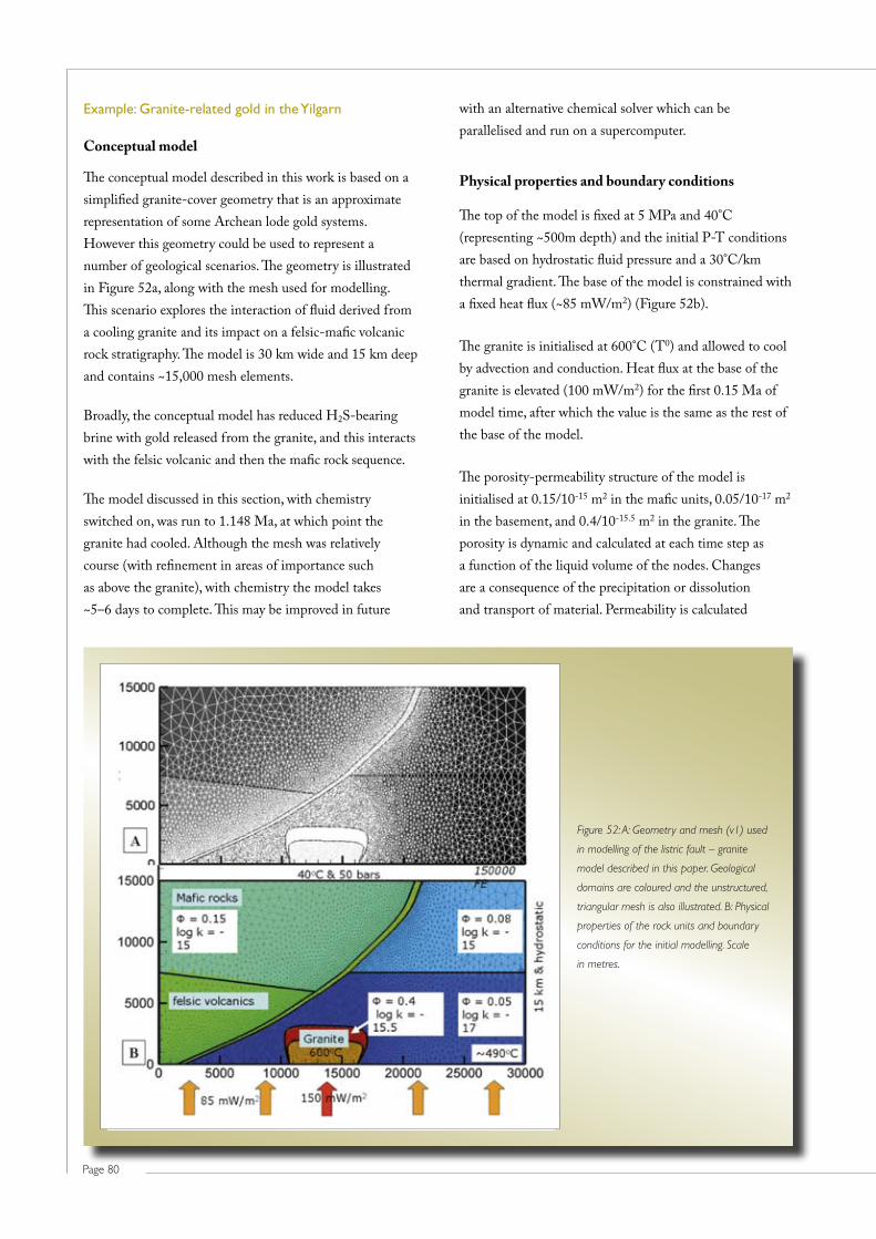
Page 80
with an alternative chemical solver which can be parallelised and run on a supercomputer.
Physical properties and boundary conditions
The top of the model is fixed at 5 MPa and 40°C (representing ~500m depth) and the initial P-T conditions are based on hydrostatic fluid pressure and a 30°C/km thermal gradient. The base of the model is constrained with a fixed heat flux (~85 mW/m2) (Figure 52b).
The granite is initialised at 600°C (T0) and allowed to cool by advection and conduction. Heat flux at the base of the granite is elevated (100 mW/m2) for the first 0.15 Ma of model time, after which the value is the same as the rest of the base of the model.
The porosity-permeability structure of the model is initialised at 0.15/10-15 m2 in the mafic units, 0.05/10-17 m2 in the basement, and 0.4/10-15.5 m2 in the granite. The porosity is dynamic and calculated at each time step as a function of the liquid volume of the nodes. Changes are a consequence of the precipitation or dissolution and transport of material. Permeability is calculated
Example: Granite-related gold in the Yilgarn
Conceptual model
The conceptual model described in this work is based on a simplified granite-cover geometry that is an approximate representation of some Archean lode gold systems. However this geometry could be used to represent a number of geological scenarios. The geometry is illustrated in Figure 52a, along with the mesh used for modelling. This scenario explores the interaction of fluid derived from a cooling granite and its impact on a felsic-mafic volcanic rock stratigraphy. The model is 30 km wide and 15 km deep and contains ~15,000 mesh elements.
Broadly, the conceptual model has reduced H2S-bearing brine with gold released from the granite, and this interacts with the felsic volcanic and then the mafic rock sequence.
The model discussed in this section, with chemistry switched on, was run to 1.148 Ma, at which point the granite had cooled. Although the mesh was relatively course (with refinement in areas of importance such as above the granite), with chemistry the model takes ~5–6 days to complete. This may be improved in future
Figure 52: A: Geometry and mesh (v1) used
in modelling of the listric fault – granite
model described in this paper. Geological
domains are coloured and the unstructured,
triangular mesh is also illustrated. B: Physical
properties of the rock units and boundary
conditions for the initial modelling. Scale
in metres.

Page 81
pmd*CRC ProjeCtS M4, M9 and F6 Final rePort
Evolution in space
Thermal-Flow Evolution
Figure 53 illustrates a composite of the thermal and flow fields at 0.15 Ma (active gold deposition) showing the magmatic tracer, flow vectors and temperature. The model’s most striking feature is the large-scale thermal and mass plume above the granite, even when it has cooled significantly (100°C above background at 0.15 Ma). This upwelling causes localisation of convection in the overlying basin, although convection is likely a consequence of the overall thermal gradient in the model and not just the granite interaction. Localisation is also a function of the chemically-influenced porosity/permeability changes (see below).
Thermal modelling without chemistry is relatively quick (models can take a few hours) allowing the effect of varying model parameters (e.g. initial permeability) to be explored. The DMT can be used to submit multiple models to supercomputing facilities (such as iVEC, in Perth) to quickly model a large range of parameters. An extension of this work, with a finer mesh resolution, has been used to explore the influence of thermal gradient (10–40°C) with the presence of granite at different temperatures
as a function of porosity using the Carman-Kozeny relationship, κ = κ0(φ/φ0)3.
Chemistry
Initial solid and aqueous chemistries were defined for each of the model units. The mineralogy is:
• Maficunit:albite–quartz–calcite–tremolite–chlorite – pyrrhotite – graphite;
• Felsicvolcanics:quartz-albite-muscovite-k-feldspar-pyrite;
• Granite:quartz-albite/anorthite-k-feldspar-biotite-magnetite with H2S in the fluid.
The fluid phase is populated initially with a mixed brine (Na, K, Ca, Fe) at ratios close to equilibrium for that rock, H2S±SO4, Au+ (1e-9 and 1e-5 molal for background & granite respectively), and CO2. The ΣC(aq) is minor in the mafic rocks (CH4), dominant in the felsic volcanics (CO2) and absent in the granite. The initial chemical step (with no transport) defines the fluid composition that is in full equilibrium with the rock. The equilibrium phase assemblage will vary across lithological units due to variations in T and P.
Figure 53: Thermal and flow results
illustrated for 0.15 Ma showing (A) tracer
from granite and flow vectors and, (B) the
temperature field (°C). Scale in metres.
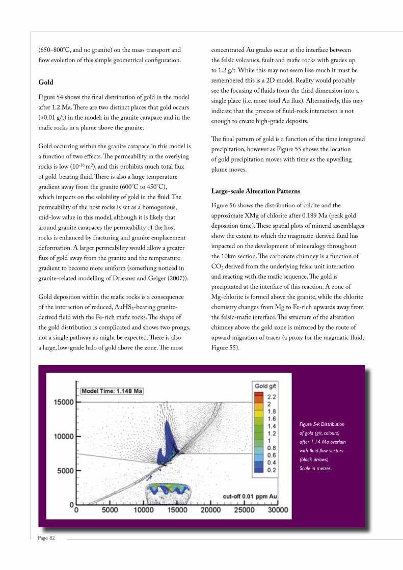
Page 82
concentrated Au grades occur at the interface between the felsic volcanics, fault and mafic rocks with grades up to 1.2 g/t. While this may not seem like much it must be remembered this is a 2D model. Reality would probably see the focusing of fluids from the third dimension into a single place (i.e. more total Au flux). Alternatively, this may indicate that the process of fluid-rock interaction is not enough to create high-grade deposits.
The final pattern of gold is a function of the time integrated precipitation, however as Figure 55 shows the location of gold precipitation moves with time as the upwelling plume moves.
Large-scale Alteration Patterns
Figure 56 shows the distribution of calcite and the approximate XMg of chlorite after 0.189 Ma (peak gold deposition time). These spatial plots of mineral assemblages show the extent to which the magmatic-derived fluid has impacted on the development of mineralogy throughout the 10km section. The carbonate chimney is a function of CO2 derived from the underlying felsic unit interaction and reacting with the mafic sequence. The gold is precipitated at the interface of this reaction. A zone of Mg-chlorite is formed above the granite, while the chlorite chemistry changes from Mg to Fe-rich upwards away from the felsic-mafic interface. The structure of the alteration chimney above the gold zone is mirrored by the route of upward migration of tracer (a proxy for the magmatic fluid; Figure 55).
(650–800°C, and no granite) on the mass transport and flow evolution of this simple geometrical configuration.
Gold
Figure 54 shows the final distribution of gold in the model after 1.2 Ma. There are two distinct places that gold occurs (>0.01 g/t) in the model: in the granite carapace and in the mafic rocks in a plume above the granite.
Gold occurring within the granite carapace in this model is a function of two effects. The permeability in the overlying rocks is low (10-16 m2), and this prohibits much total flux of gold-bearing fluid. There is also a large temperature gradient away from the granite (600°C to 450°C), which impacts on the solubility of gold in the fluid. The permeability of the host rocks is set as a homogenous, mid-low value in this model, although it is likely that around granite carapaces the permeability of the host rocks is enhanced by fracturing and granite emplacement deformation. A larger permeability would allow a greater flux of gold away from the granite and the temperature gradient to become more uniform (something noticed in granite-related modelling of Driesner and Geiger (2007)).
Gold deposition within the mafic rocks is a consequence of the interaction of reduced, AuHS2-bearing granite-derived fluid with the Fe-rich mafic rocks. The shape of the gold distribution is complicated and shows two prongs, not a single pathway as might be expected. There is also a large, low-grade halo of gold above the zone. The most
Figure 54: Distribution
of gold (g/t, colours)
after 1.14 Ma overlain
with fluid-flow vectors
(black arrows).
Scale in metres.

Page 83
pmd*CRC ProjeCtS M4, M9 and F6 Final rePort
Figure 55: Evolution of the tracer (proxy for magmatic fluid) at the interface
between mafic-felsic units and the fault at (A) 0.189 Ma and, (B) 0.784 Ma.
The precipitated gold is illustrated by black contours, which show the final gold
distribution is a function of the integrated passage of tracer through time. History
point relates to Figure 58. Scale in metres.
Figure 56: (A) Distribution of calcite after 0.189 Ma. Note
steep carbonate plume in mafic rocks above the granite.
(B) Calculated chlorite chemistry (XMg). Scale in metres.

Page 84
from the chemical reactions (i.e. addition of carbonate). Figure 57 shows the permeability distribution in this area at 0.784 Ma showing a change of an order of magnitude (10-15.5 to 10-14.5 m2) related to chemical precipitation and dissolution.
Simulated Paragenesis
Figure 57 contains a dot at the intersection of the magmatic fluid with the mafic rock units. This point has been used to generate a history of minerals through time and is presented as a stacked plot (cm3) in Figure 58. The initial assemblage consisting of quartz-epidote-chlorite-albite with minor carbonate-tremolite sees tremolite
Evolution in Time
Magmatic Upwelling
The position of the tracer away from the granite is not a single static upwelling but evolves in space through time. Figure 55 shows two time snapshots of the magmatic tracer at the interface between the felsic and mafic rock units (along with the fault). In this example the locus of magmatic upwelling has migrated laterally ~3km between 0.189 and 0.784 Ma. This is a function of the coupling between convective flow in the upper geological units effectively pushing the plume around and changes in the permeability of the host rock due to feedback
Figure 58: Evolution of mineral
abundance (volume) over time at the
history point shown in Figure 57. The
gold concentration is a black line. This
is a stacked plot so variation in totals
equates to variation in the bulk solid
volume (1/porosity) value.
Figure 57: Permeability values and flow arrows for the critical
interface region at 0.784 Ma, showing that the mafic units with initial
permeability of 10-15 m2 have evolved through chemical reaction to
a range between 10-14 and 10-15 m2. White dot is the history point
used in Figure 58. Scale in metres.
Page 85
pmd*CRC ProjeCtS M4, M9 and F6 Final rePort
prediction in mineral systems. In: SGA2007 Dublin, Society for Geology Applied to Mineral Deposits.
Cleverley JS & Bastrakov EN (2005) K2GWB: Utility for generating thermodynamic data files for The Geochemist’s Workbench (R) at 0–1000 degrees C and 1–5000 bar from UT2K and the UNITHERM database. Computers & Geosciences, 31, 756–767.
Cleverley JS, Hornby P & Poulet T (2006) Reactive transport modelling in hydrothermal systems using the Gibbs minimisation approach. Geochimica Et Cosmochimica Acta, 70, A106–A106.
Driesner T & Geiger S (2007) Numerical simulation of multiphase fluid flow in hydrothermal systems. In: Fluid-Fluid Interactions eds Liebscher A & Heinrich CA), Mineralogical Society of America, 65.
Shvarov YV & Bastrakov EN (1999) HCh: a software package for geochemical equilibrium modelling. User’s Guide. Canberra, Australian Geological Survey Organisation.
2.13 Using Reactive Transport Models to Predict the Geophysical Responses of Alteration
Richard Chopping and James S. Cleverley
Introduction
Geophysical responses, such as gravity, total magnetic intensity or seismic reflections, result from spatial variations in physical properties, such as density, magnetic susceptibility or acoustic impedance, of the present-day subsurface. The physical properties of the subsurface are a function of the region’s prior geological history. In basement terranes, where most mineral deposits are found, the physical properties are primarily controlled by the mineralogy of the rocks in the subsurface. This mineralogy is controlled by primary lithology as well as a chemical alteration overprint.
The reactive transport (RT) modelling code, through its simulations of heat and fluid flow, and chemical reactions, produces models of mineralogy that vary spatially and temporally (see section 2.12). These models of mineralogy can be used to produce physical property models and predict the geophysical response of the alteration system simulated by the RT model.
disappear, quartz, chlorite and carbonate increase and, muscovite replace epidote during the phase of active gold deposition. This paragenesis is testable in real examples. In later stages the quartz and carbonate continue to increase, albite disappears and muscovite is reconverted to epidote. Graphite also starts to dominate in the later stages as the reduced mafic derived fluids interact with the oxidised CO2 bearing deeper fluids. This has implications for the modelling or consideration of the isotopic signals of these products in this process (i.e. mixed carbon sources at different redox states).
The gold is actively precipitated over the period 0.71 – 0.51 Ma in this location. The precipitation of gold at other locations would have occurred at different times but all within 1 Ma. While these time differences would bedifficulttoresolvewithinArcheandeposits,thismayimpact on our understanding of recent systems (<50 Ma), where geochronology has a better resolution.
Conclusions
The RT code can be used to develop and run combinations of thermal-flow-transport and chemical reaction models (reactive transport couples all these processes). The code is run using the DMT interface and by the end of the pmd*CRC at least the thermal-transport models can be run using the supercomputing facilities available on the grid.
The model discussed here explores the interaction between granite derived, Au-H2S-bearing fluid and felsic basement and overlying mafic sequence. The geometry and chemistry of the units is loosely applicable to many Yilgarn-type scenarios. In this model the granite causes focused upflow of mass and heat, but there is little influence on this upwelling plume by the fault. During the passage of the fluid through the felsic basement the fluid maintains the reduced, Au-bearing capacity, while interaction with the mafic sequence causes processes of reduction-oxidation (by fluid-rock and fluid-fluid interaction) to precipitate gold and associated assemblages, including muscovite-carbonate. Carbonate maps out the upwelling plume and has been used to model the gravity lows around some Yilgarn gold systems (see section 2.13).
References
Cleverley JS (2007) Large scale finite element reactive transport modelling as a tool to aid understanding and

Page 86
mineral component of the mineralogy. The density of any given point within the RT model is:
The gravity response depends also on the density contrast with respect to the entire crust. Most gravity maps are based on the Bouguer corrected gravity, which assumes a constant crustal density of 2670 kgm-3 (Telford et al., 1990). To produce a physical property model which would simulate the Bouguer response, the bulk density calculated using the above formula needs to be corrected to the Bouguer density: Bouguer density contrast = bulk density – 2670 kgm-3.
Magnetic susceptibility
Magnetic susceptibility is a dimensionless constant that relates the inducing magnetic field to the magnetic field due to a magnetic material. Although it is dimensionless, it has a different scale in SI compared to cgs units: Susceptibilities for cgs units are 4π smaller than SI susceptibilities (i.e. 1 cgs unit = SI unit / 4π: Whiting, 1986, Telford et al., 1990).
Magnetic susceptibilities are predominantly influenced by magnetite, ilmenite and/or pyrrhotite content, which are the three most ferromagnetic minerals. Some paramagnetic materials, such as quartz, have negligible to negative magnetic susceptibilities. Generally, for modelling magnetic response these are assumed to be particularly small, that is, kquartz ~ 10-7 to 10-9 in SI units (Williams and Dipple, 2006).
The simplest way to calculate the magnetic susceptibility from mineralogy is to assume it is a linear average, weighted by the volumetric proportion of each mineral, of the magnetic susceptibility of each mineral:
This formula is appropriate for concentrations of magnetite up to ~ 20% by volume. Above this, the magnetic domains do not combine linearly (Shandley and Bacon, 1966; Fannin et al., 1990).
n
i i
i
vol
massdensitybulk
0
n
iin
ii
i k
vol
volk
0
0
This summary describes a method to calculate the geophysical response of a RT model, and a simple example of applying it to a model simulating gold deposition (Cleverley et al., 2006). More detailed analysis of the possible geophysical signatures of this model are given by Chopping (2008); a comparison of these signatures with a known mineralised region are discussed by Chopping et al. (2008).
Creating physical property models from an RT model
A number of methods to calculate physical properties from mineralogy exists in the published literature. We will discuss some of these methods for three key physical properties: density, magnetic susceptibility and seismic velocity.
Density
Density, defined as the mass per unit volume of material, is the simplest physical property to calculate, and thus is not discussed in the literature. If its calculation does not include porosity, then the calculated density is the bulk or material density (Emerson, 1990). For the purposes of using gravity surveys in the exploration of mineral deposits, the bulk density is the property required to calculate the gravity response.
Reactive transport models specify the mineralogy of the solid phases in terms of the number of moles of each mineral. Defined in the chemical system specification of the model is the molar volume and mass for each mineral, which can be used to calculate the mass and volume of each
Notation
i Arbitrary mineral index, assuming an array of minerals; subscript on various properties relates to that property for a given mineral
n Number of minerals that constitute the mineralogy of a cell in the RT model
k Magnetic susceptibility
v Seismic velocity
vp (or vs) P- (or S-) wave velocity

Page 87
pmd*CRC ProjeCtS M4, M9 and F6 Final rePort
RT model must be sampled on a regular grid14. A suitable interpolation method to preserve the resolution and limit the introduction of artefacts is the natural neighbour algorithm (Owen, 1992).
For 2D RT models, the regular grid must be extended into the third dimension to calculate the gravity response. There may also be edge effects that result from mass changes off to the side; in this case, it is desirable to mirror the physical property model on either side.
The seismic response of the RT model is considerably more complex to forward-model than the gravity or magnetic responses. One simple way to image where reflections may arise from an arbitrary acoustic impedance model is to examine a vertical reflection profile. To calculate this, the reflectioncoefficientofeachcellisrelatedtotheacousticimpedance of a cell (depth z, horizontal position xy) and the cell immediately below it (depth z+1, horizontal position xy):
Tointerprettheverticalreflectioncoefficientmodel,reflectioncoefficientsgreaterthan0.06,ingeneral,willresult in a strong positive reflection, and a reflection coefficientsmallerthan-0.06willresultinastrongnegative reflection (assuming vertical incidence, Salisbury et al., 2000). More complex methods to calculate the seismic response of an RT model are beyond the scope of this summary report (for a possible scheme see Hobbs, 2003).
An example: the gravity response of an RT model
For this example we used the listric fault model of Cleverley et al. (2006), created physical property distributions, and calculated the density response for a gold deposit presently sitting at the base of 100m of constant low-density (2000 kgm-3) material, to simulate the regolith. The initial RT model was used to simulate an unaltered architecture, and the RT model after chemical alteration and fluid transport was used to simulate an architecture
14 The voxels within the 3D property distribution need not be cubic for the grav3d and mag3d codes. They can have rectangular sizes, and the cells can be of variable size throughout the property volume. To preserve the spatial resolution of the RT model, however, it is advisable to have cells with side lengths similar to the spacing of the closest nodes in the RT model.
1
1
xyzxyz
xyzxyzxyz ZZ
ZZR
Other empirically-derived formulae exist to calculate magnetic susceptibility based on magnetite content (e.g. Werner, 1945; Mooney and Bleifuss, 1953; Grant and West, 1965; Parasnis, 1973). These methods can be applied to the proportion of all magnetic minerals by using magnetite-equivalent volumes (Shandley and Bacon, 1966): volmagnetite equivalent = voli × (ki/kmagnetite).
This magnetite-equivalent volume may then be used in place of the magnetite volume in any method that is only based on the volume proportion of magnetite.
Seismic Velocity
Similarly to magnetic susceptibilities, the seismic velocity of an arbitrary mineralogy can be calculated using linear averaging, weighted by the volume of the minerals:
Another method, generally named the time-averaged method (Wyllie et al., 1956), is to linearly average the slowness (1/v) of each of the minerals:
More elaborate schemes exist for calculating seismic velocity from mineralogy. Voigt-Reuss-Hill (in Berryman, 1995) or Hashin-Shtrikman (in Watt, 1988) use the elastic moduli of the minerals. For minerals of mantle origin, the elastic moduli are well defined – they are required inputs to chemical understandings from regional and whole-earth seismic tomography – they are not well defined for crustal minerals. The linear and time-averaged methods produce similar results, with subtle differences; our preferred choice is slightly simpler to conceptualise linear averaging method to calculate seismic velocity.
Calculating the model’s geophysical responses
Calculating the gravity and magnetic response can be performed using the forward-modelling components of the University of British Columbia – Geophysical Inversion Facility (UBC-GIF) potential field inversion codes grav3d (Li and Oldenburg, 1998) and mag3d (Li and Oldenburg, 1996). To calculate the gravity, or magnetic, response, the
n
iin
ii
i v
vol
volv
0
0
n
ii
n
ii
i
vvol
vol
v 0
0
1
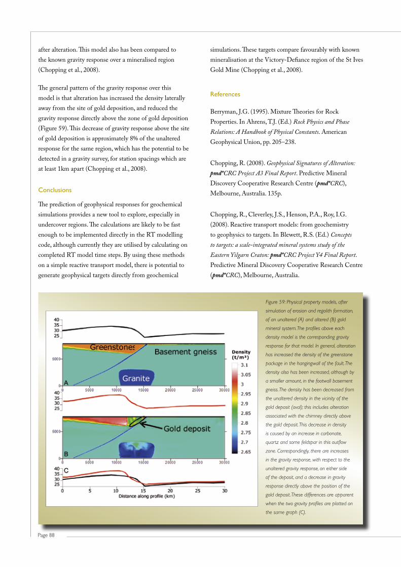
Page 88
simulations. These targets compare favourably with known mineralisation at the Victory-Defiance region of the St Ives Gold Mine (Chopping et al., 2008).
References
Berryman, J.G. (1995). Mixture Theories for Rock Properties. In Ahrens, T.J. (Ed.) Rock Physics and Phase Relations: A Handbook of Physical Constants. American Geophysical Union, pp. 205–238.
Chopping, R. (2008). Geophysical Signatures of Alteration: pmd*CRC Project A3 Final Report. Predictive Mineral Discovery Cooperative Research Centre (pmd*CRC), Melbourne, Australia. 135p.
Chopping, R., Cleverley, J.S., Henson, P.A., Roy, I.G. (2008). Reactive transport models: from geochemistry to geophysics to targets. In Blewett, R.S. (Ed.) Concepts to targets: a scale-integrated mineral systems study of the Eastern Yilgarn Craton: pmd*CRC Project Y4 Final Report. Predictive Mineral Discovery Cooperative Research Centre (pmd*CRC), Melbourne, Australia.
after alteration. This model also has been compared to the known gravity response over a mineralised region (Chopping et al., 2008).
The general pattern of the gravity response over this model is that alteration has increased the density laterally away from the site of gold deposition, and reduced the gravity response directly above the zone of gold deposition (Figure 59). This decrease of gravity response above the site of gold deposition is approximately 8% of the unaltered response for the same region, which has the potential to be detected in a gravity survey, for station spacings which are at least 1km apart (Chopping et al., 2008).
Conclusions
The prediction of geophysical responses for geochemical simulations provides a new tool to explore, especially in undercover regions. The calculations are likely to be fast enough to be implemented directly in the RT modelling code, although currently they are utilised by calculating on completed RT model time steps. By using these methods on a simple reactive transport model, there is potential to generate geophysical targets directly from geochemical
Figure 59: Physical property models, after
simulation of erosion and regolith formation,
of an unaltered (A) and altered (B) gold
mineral system. The profiles above each
density model is the corresponding gravity
response for that model. In general, alteration
has increased the density of the greenstone
package in the hangingwall of the fault. The
density also has been increased, although by
a smaller amount, in the footwall basement
gneiss. The density has been decreased from
the unaltered density in the vicinity of the
gold deposit (oval); this includes alteration
associated with the chimney directly above
the gold deposit. This decrease in density
is caused by an increase in carbonate,
quartz and some feldspar in this outflow
zone. Correspondingly, there are increases
in the gravity response, with respect to the
unaltered gravity response, on either side
of the deposit, and a decrease in gravity
response directly above the position of the
gold deposit. These differences are apparent
when the two gravity profiles are plotted on
the same graph (C).
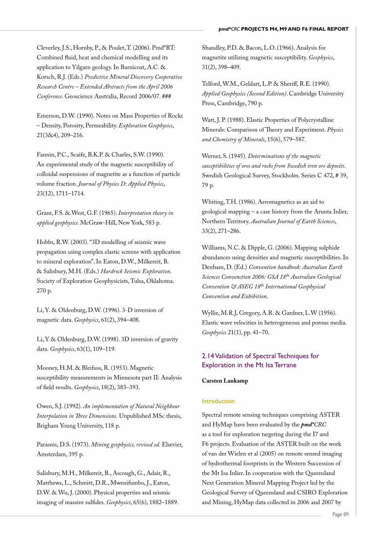
Page 89
pmd*CRC ProjeCtS M4, M9 and F6 Final rePort
Shandley, P.D. & Bacon, L.O. (1966). Analysis for magnetite utilizing magnetic susceptibility. Geophysics, 31(2), 398–409.
Telford, W.M., Geldart, L.P. & Sheriff, R.E. (1990). Applied Geophysics (Second Edition). Cambridge University Press, Cambridge, 790 p.
Watt, J. P. (1988). Elastic Properties of Polycrystalline Minerals: Comparison of Theory and Experiment. Physics and Chemistry of Minerals, 15(6), 579–587.
Werner, S. (1945). Determinations of the magnetic susceptibilities of ores and rocks from Swedish iron ore deposits. Swedish Geological Survey, Stockholm. Series C 472, # 39, 79 p.
Whiting, T.H. (1986). Aeromagnetics as an aid to geological mapping – a case history from the Arunta Inlier, Northern Territory. Australian Journal of Earth Sciences, 33(2), 271–286.
Williams, N.C. & Dipple, G. (2006). Mapping sulphide abundances using densities and magnetic susceptibilities. In Denham, D. (Ed.) Convention handbook: Australian Earth Sciences Convenction 2006: GSA 18th Australian Geological Convention & ASEG 18th International Geophysical Convention and Exhibition.
Wyllie, M.R.J, Gregory, A.R. & Gardner, L.W (1956). Elastic wave velocities in heterogeneous and porous media. Geophysics 21(1), pp. 41–70.
2.14 Validation of Spectral Techniques for Exploration in the Mt Isa Terrane
Carsten Laukamp
Introduction
Spectral remote sensing techniques comprising ASTER and HyMap have been evaluated by the pmd*CRC as a tool for exploration targeting during the I7 and F6 projects. Evaluation of the ASTER built on the work of van der Wielen et al (2005) on remote sensed imaging of hydrothermal footprints in the Western Succession of the Mt Isa Inlier. In cooperation with the Queensland Next Generation Mineral Mapping Project led by the Geological Survey of Queensland and CSIRO Exploration and Mining, HyMap data collected in 2006 and 2007 by
Cleverley, J.S., Hornby, P., & Poulet, T. (2006). Pmd*RT: Combined fluid, heat and chemical modelling and its application to Yilgarn geology. In Barnicoat, A.C. & Korsch, R.J. (Eds.) Predictive Mineral Discovery Cooperative Research Centre – Extended Abstracts from the April 2006 Conference. Geoscience Australia, Record 2006/07. ###
Emerson, D.W. (1990). Notes on Mass Properties of Rocks – Density, Porosity, Permeability. Exploration Geophysics, 21(3&4), 209–216.
Fannin, P.C., Scaife, B.K.P. & Charles, S.W. (1990). An experimental study of the magnetic susceptibility of colloidal suspensions of magnetite as a function of particle volume fraction. Journal of Physics D: Applied Physics, 23(12), 1711–1714.
Grant, F.S. & West, G.F. (1965). Interpretation theory in applied geophysics. McGraw-Hill, New York, 583 p.
Hobbs, R.W. (2003). “3D modelling of seismic wave propagation using complex elastic screens with application to mineral exploration”. In Eaton, D.W., Milkereit, B. & Salisbury, M.H. (Eds.) Hardrock Seismic Exploration. Society of Exploration Geophysicists, Tulsa, Oklahoma. 270 p.
Li, Y. & Oldenburg, D.W. (1996). 3-D inversion of magnetic data. Geophysics, 61(2), 394–408.
Li, Y & Oldenburg, D.W. (1998). 3D inversion of gravity data. Geophysics, 63(1), 109–119.
Mooney, H.M. & Bleifuss, R. (1953). Magnetic susceptibility measurements in Minnesota part II: Analysis of field results. Geophysics, 18(2), 383–393.
Owen, S.J. (1992). An implementation of Natural Neighbour Interpolation in Three Dimensions. Unpublished MSc thesis, Brigham Young University, 118 p.
Parasnis, D.S. (1973). Mining geophysics, revised ed. Elsevier, Amsterdam, 395 p.
Salisbury, M.H., Milkereit, B., Ascough, G., Adair, R., Matthews, L., Schmitt, D.R., Mwenifumbo, J., Eaton, D.W. & Wu, J. (2000). Physical properties and seismic imaging of massive sulfides. Geophysics, 65(6), 1882–1889.
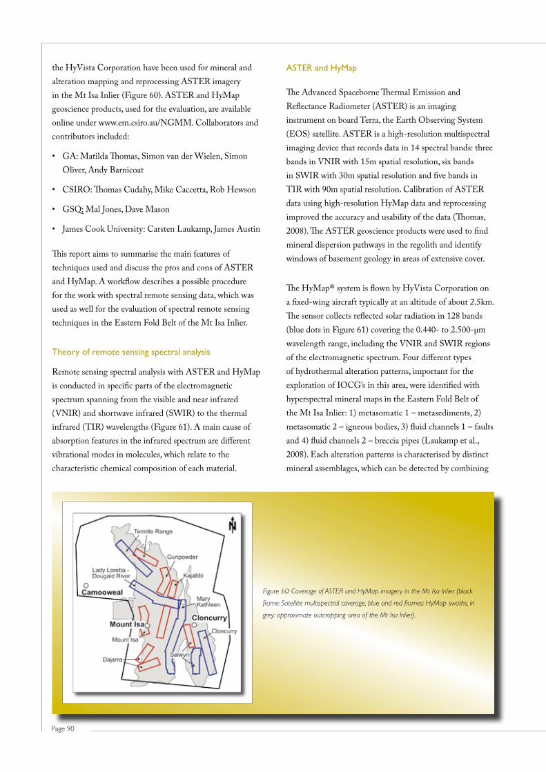
Page 90
ASTER and HyMap
The Advanced Spaceborne Thermal Emission and Reflectance Radiometer (ASTER) is an imaging instrument on board Terra, the Earth Observing System (EOS) satellite. ASTER is a high-resolution multispectral imaging device that records data in 14 spectral bands: three bands in VNIR with 15m spatial resolution, six bands in SWIR with 30m spatial resolution and five bands in TIR with 90m spatial resolution. Calibration of ASTER data using high-resolution HyMap data and reprocessing improved the accuracy and usability of the data (Thomas, 2008). The ASTER geoscience products were used to find mineral dispersion pathways in the regolith and identify windows of basement geology in areas of extensive cover.
The HyMap® system is flown by HyVista Corporation on a fixed-wing aircraft typically at an altitude of about 2.5km. The sensor collects reflected solar radiation in 128 bands (blue dots in Figure 61) covering the 0.440- to 2.500-μm wavelength range, including the VNIR and SWIR regions of the electromagnetic spectrum. Four different types of hydrothermal alteration patterns, important for the exploration of IOCG’s in this area, were identified with hyperspectral mineral maps in the Eastern Fold Belt of the Mt Isa Inlier: 1) metasomatic 1 – metasediments, 2) metasomatic 2 – igneous bodies, 3) fluid channels 1 – faults and 4) fluid channels 2 – breccia pipes (Laukamp et al., 2008). Each alteration patterns is characterised by distinct mineral assemblages, which can be detected by combining
the HyVista Corporation have been used for mineral and alteration mapping and reprocessing ASTER imagery in the Mt Isa Inlier (Figure 60). ASTER and HyMap geoscience products, used for the evaluation, are available online under www.em.csiro.au/NGMM. Collaborators and contributors included:
• GA:MatildaThomas,SimonvanderWielen,SimonOliver, Andy Barnicoat
• CSIRO:ThomasCudahy,MikeCaccetta,RobHewson
• GSQ:MalJones,DaveMason
• JamesCookUniversity:CarstenLaukamp,JamesAustin
This report aims to summarise the main features of techniques used and discuss the pros and cons of ASTER and HyMap. A workflow describes a possible procedure for the work with spectral remote sensing data, which was used as well for the evaluation of spectral remote sensing techniques in the Eastern Fold Belt of the Mt Isa Inlier.
Theory of remote sensing spectral analysis
Remote sensing spectral analysis with ASTER and HyMap is conducted in specific parts of the electromagnetic spectrum spanning from the visible and near infrared (VNIR) and shortwave infrared (SWIR) to the thermal infrared (TIR) wavelengths (Figure 61). A main cause of absorption features in the infrared spectrum are different vibrational modes in molecules, which relate to the characteristic chemical composition of each material.
Figure 60: Coverage of ASTER and HyMap imagery in the Mt Isa Inlier (black
frame: Satellite multispectral coverage, blue and red frames: HyMap swaths, in
grey: approximate outcropping area of the Mt Isa Inlier).

Page 91
pmd*CRC ProjeCtS M4, M9 and F6 Final rePort
Evaluation of ASTER and HyMap
Major differences of ASTER in HyMap, which are important for exploration, are the spectral and spatial coverage, and spectral and spatial resolution.
ASTER covers with additional five bands partly the TIR part of the electromagnetic spectrum, enabling detection of major mineral phases, such as quartz and feldspars, and enhancing the possibility for the detection of carbonates and sulphates. This part of the electromagnetic spectrum is not covered by the HyMap system used in the Mt Isa Inlier.
Calibration of the ASTER data with the new HyMap data and cross-calibration of the single ASTER scenes led to an ASTER mosaic, which almost covers almost the entire Mt Isa Inlier (Thomas, 2008) and enables comparison of various locations in this area. However, contrasting growth in vegetation in different years and seasonal differences in vegetation cover (dry and green) cause persistent problematical errors in the ASTER mosaic. The mineral information processing of the HyMap reflectance data was based on CSIRO’s “C-HyperMAP” software package, which was developed to handle large-volume, multi-scene hyperspectral imagery. C-HyperMAP runs as an add-on to IDL-ENVI™ (http://www.ittvis.com) to capture the benefits of ENVI’s image display and other functionality. The procedure for mineral information extraction using C-HyperMAP is based on measuring the diagnostic absorption bands, including their depths, wavelengths and geometries (full-width half height and asymmetry).
hyperspectral mineral maps and other geophysical-geochemical spatial data.
Processing, such as masking and application of different stretch modes, of ASTER and HyMap raw data can be done with the RSI ENVI 4.3 software or in a limited way with ER Mapper software.
PIMA
The portable infrared mineral analyser (PIMA) was used for ground validation of HyMap and ASTER data. PIMA can be used to analyse small sample areas of ca. 15mm in diameter. The PIMA measures reflected radiation in the SWIR-range (1.3 -2.5µm) and can detect a limited range of minerals such as chlorite, mica, sulphates and carbonate. PIMA analyses were largely backed up with XRD/XRF and GADDS analyses at the Advanced Analytical Centre of the James Cook University in Townsville.
PIMA analysis is a quick, easy method, but the handling of the PIMA in the field is not very convenient. It should also be noted PIMA cannot detect major phases such as Qtz and Fsp. Another problem analysing relatively dark rocks, such as shale or gabbro, is their largely aspectral mineral assemblage that can’t be detected by the PIMA. Results from dark rocks/minerals can be significantly improved by adjusting the PIMA SP/RAP acquisition software. One way to do this is to enhance the factor of integration from 1 to 4, which comes along with a respective prolongation of the measurement period.
Figure 61: Spectral-Mineral
Wavelength Regions
(courtesy Peter Hausknecht)
with HyMap bands
represented by blue dots and
ASTER bands represented
by black bars. Examples
of detectable minerals are
given in the top part of
the diagram. Examples of
common rock types, dark soil
and selected vegetation are
represented by the respective
absorption spectra.
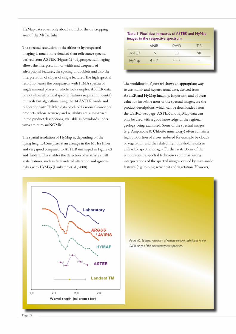
Page 92
The workflow in Figure 64 shows an appropriate way to use multi- and hyperspectral data, derived from ASTER and HyMap imaging. Important, and of great value for first-time users of the spectral images, are the product descriptions, which can be downloaded from the CSIRO webpage. ASTER and HyMap data can only be used with a good knowledge of the regional geology being examined. Some of the spectral images (e.g. Amphibole & Chlorite mineralogy) often contain a high proportion of errors, induced for example by clouds or vegetation, and the related high threshold results in unfeasible spectral images. Further restrictions of the remote sensing spectral techniques comprise wrong interpretations of the spectral images, caused by man-made features (e.g. mining activities) and vegetation. However,
Table 1: Pixel size in metres of ASTER and HyMap images in the respective spectrum.
VNIR SWIR TIR
ASTER 15 30 90
HyMap 4 – 7 4 – 7 –
HyMap data cover only about a third of the outcropping area of the Mt Isa Inlier.
The spectral resolution of the airborne hyperspectral imaging is much more detailed than reflectance spectra derived from ASTER (Figure 62). Hyperspectral imaging allows the interpretation of width and deepness of adsorptional features, the spacing of doublets and also the interpretation of slopes of single features. The high spectral resolution eases the comparison with PIMA spectra of single mineral phases or whole rock samples. ASTER data do not show all critical spectral features required to identify minerals but algorithms using the 14 ASTER bands and calibration with HyMap data produced various Geoscience products, whose accuracy and reliability are summarised in the product descriptions, available as downloads under www.em.csiro.au/NGMM.
The spatial resolution of HyMap is, depending on the flying height, 4.5m/pixel at an average in the Mt Isa Inlier and very good compared to ASTER envisaged in Figure 63 and Table 1. This enables the detection of relatively small scale features, such as fault-related alteration and igneous dykes with HyMap (Laukamp et al., 2008).
Figure 62: Spectral resolution of remote sensing techniques in the
SWIR range of the electromagnetic spectrum.
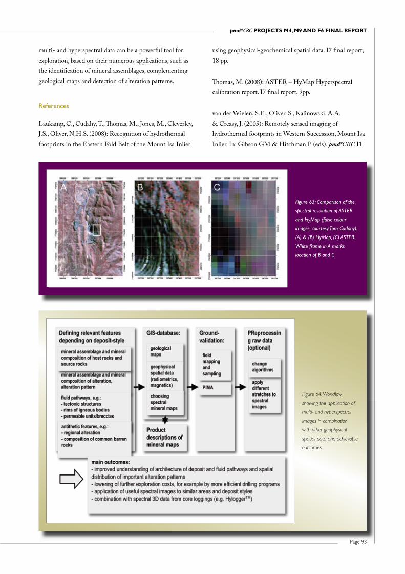
Page 93
pmd*CRC ProjeCtS M4, M9 and F6 Final rePort
using geophysical-geochemical spatial data. I7 final report, 18 pp.
Thomas, M. (2008): ASTER – HyMap Hyperspectral calibration report. I7 final report, 9pp.
van der Wielen, S.E., Oliver. S., Kalinowski. A.A. & Creasy, J. (2005): Remotely sensed imaging of hydrothermal footprints in Western Succession, Mount Isa Inlier. In: Gibson GM & Hitchman P (eds). pmd*CRC I1
multi- and hyperspectral data can be a powerful tool for exploration, based on their numerous applications, such as the identification of mineral assemblages, complementing geological maps and detection of alteration patterns.
References
Laukamp, C., Cudahy, T., Thomas, M., Jones, M., Cleverley, J.S., Oliver, N.H.S. (2008): Recognition of hydrothermal footprints in the Eastern Fold Belt of the Mount Isa Inlier
Figure 63: Comparison of the
spectral resolution of ASTER
and HyMap (false colour
images, courtesy Tom Cudahy).
(A) & (B) HyMap, (C) ASTER.
White frame in A marks
location of B and C.
Figure 64: Workflow
showing the application of
multi- and hyperspectral
images in combination
with other geophysical
spatial data and achievable
outcomes.

Page 94
developing a quantitative science base for understanding multiscale observations in chemistry and mechanics, from grain size to plate scale processes. These are the first steps to developing a numerical framework to model the mechanics/chemistry of fluid transfer through the deep (ductile) realm, complementing the modelling of fluid flow in the shallow (brittle) crust that has become well-established within the pmd*CRC. This deep-seated fluid generation and transfer mechanism drives the genesis of giant ore deposits within the shallow crust. The next step is to add the fundamental link from nano-scale to plate scale within one self-consistent thermodynamic framework.
A non-equilibrium thermodynamic approach to crustal deformation is being explored as a way to understand mineralsystems. It includes a fully coupled solution to the energy, momentum and continuity equations of the system, allowing the prediction of fractures, shear zones and other typical geological patterns out of a randomly perturbed initial state. This approach links large-scale geodynamic processes to the underlying micro-scale processes. The key postulate underlying this approach is that large mineral deposits arise from systems that maximise their entropy production through the action of coupled processes that dissipate energy (Hobbs et al., 2007). These processes include deformation, fluid transport, heat transport and chemical reactions.
Planetary to tectonic plate-scale behaviours predicted by a computational approach based on a self-consistent thermodynamic framework are described by Regenauer-Lieb and co-workers (Regenauer-Lieb and Yuen, 2003; Regenauer-Lieb et al., 2005). Over the past two years, these concepts and algorithms have been explored at the metre to micron scales (Hobbs et al., 2007a).
Dissipative processes involving thermal-mechanical coupling (Hobbs et al., 2007a) produce fold systems (Figure 65) with characteristics similar to those observed in the middle to lower crust. These comprise folds in layers with little strength contrast, scale invariance, no strict periodicity, small wavelength/thickness ratios, non-concentric fold shapes, and axial plane crenulations. This contrasts with classical folding theory that requires large mechanical contrasts between a weak matrix and strong embedded layers to produce periodic concentric fold systems with no formal link to axial plane structures. Folds
Project Final Report – 3D Basin Architecture and Minerals Systems in the Mt Isa Western Succession. Unpublished report, 268; pp 177–185.
2.15 A Thermodynamically Consistent Multi-scale Approach to Mineralising Systems
Alison Ord, Bruce E. Hobbs and Klaus Regenauer-Lieb
Formation of the Earth’s crust and its mineral resources involves the interplay of mechanical, thermal, hydrological and chemical processes across an extreme range of space and time. The pmd*CRC research effort has applied modelling codes designed for engineering applications to mineralising processes. This approach has been effective to date for prediction in the shallow crust. To simulate geological processes through the whole of the crust and mantle, however, we need to use a fundamental understanding of physics and chemistry across scales. Thus, the new science challenge is to develop the capability to simulate in a self-consistent manner all geological processes (and their associated feedbacks) within a robust, cross-scale computational approach. These processes involve mechanical, thermal and chemical interactions within the host rock and its fluids that can only be studied rigorously at small scales. It is well known, however, that small changes in chemical properties, such as a small change in crystalline water content, can impact on large-scale geological behaviours, such as plate tectonics. Equally, very large scale phenomena, such as mantle overturn events, can critically affect smaller-scale behaviours, such as the location and timing of mineralisation, hence the need for the new multi-scale paradigm in geology.
Geodynamicists have achieved most insights from thermodynamically self-consistent modelling at the large planetary scale and global tomographic interpretations. Propagation to smaller scales is a quintessential part of our initiative on scale linking of chemo-physical-thermodynamic approaches. We expect the methods of recognising, scaling and forward modelling of emergent patterns in dissipative systems will permit us to replace empirical analyses by “ab initio” style modelling.
The past four years have seen the application of recent breakthroughs in computational geodynamics to geological problems relevant to the pmd*CRC. The most recent work embeds chemistry into thermo-mechanical modelling,

Page 95
pmd*CRC ProjeCtS M4, M9 and F6 Final rePort
At the crustal scale for the Yilgarn mineralising system (Hobbs et al., 2007b) the processes that do work and hence dissipate energy are: plastic-viscous deformation; brittle deformation processes such as fault formation and slip; the introduction of fluids, both melts and non-melts, within the existing stress field, and, importantly, the flow of these fluids across gradients in temperature and chemical potential; the flow of heat into and out of the system; and chemical reactions including those associated with iso-chemical metamorphism, metasomatism and mineralisation. The dissipation of energy is expressed essentially as extra heat, and so is a strong contributor to metamorphism in the system. The heat generated by all these processes reduces the viscosity and nucleates shear zones and folding (see Regenauer-Lieb and Yuen, 2003; Hobbs et al., 2007a), unless the heat is dissipated primarily by conduction in which case evolution of the system aborts. This thermal-mechanical feedback does not kick-in unless the rock mass is at or above a critical temperature, which is characteristic of the lithology. This critical temperature at geological strain-rates is approximately 230°C for quartzites, 270°C for feldspar rich rocks, and 310°C for
formed at the kilometre scale are governed by thermal diffusivity. Folds also develop at smaller scales governed by the heterogeneous distribution of thermal conductivity arising from fluctuations in mineralogy.
Although different physical-chemical processes are operating, the structure of the laws for thermal, fluid and chemical transport are identical (Fourier’s, Darcy’s and Fick’s Laws respectively). Thus, fluid-mechanical and chemical-mechanical coupling are expected to lead to mechanical instabilities similar to those that arise from thermal-mechanical coupling. This has been illustrated by incorporating chemical reaction-diffusion processes into a thermo-mechanical framework. The energy dissipated during deformation of the layers leads to strain-softening behaviour and the resultant development of localised deformation which in turn nucleates buckles in the layer. Such chemical feed-back instabilities occur at the centimetre to micron scales, and so produce structures at these scales, as opposed to thermal feed-back instabilities that are important at the 100 to 1000 metre scales.
Figure 65: Progressive shortening of a 10-layer sequence
with initial spacing between the layers equal to layer
thickness. Temperature 550K. (A) Grid and (B) strain after
40% shortening; (C) Thermal strain after 45% shortening;
(D) Strain and (E) stress after 55% shortening (after
Hobbs et al., 2007a).

Page 96
pmd*CRC ProjeCtS M4, M9 and F6 Final rePort
References
Hobbs B.E., Regenauer-Lieb K. and Ord A., 2007a. Thermodynamics of folding in the middle to lower crust. Geology 35, 175–178.
Hobbs, B.E., Patton, R., Ord, A., Regenauer-Lieb, K, Walshe, J. and Hall, G., 2007b. A helicopter view of metamorphism in the Yilgarn mineralising system. In: Bierlein, F.P. and Knox-Robinson, C.M. (editors), 2007. Proceedings of Geoconferences (WA) Inc. Kalgoorlie ’07 Conference, 25–27 September 2007, Kalgoorlie, Western Australia. Geoscience Australia Record 2007/14, 249p. pp. 52–56.
Patton, R.L. & Watkinson, J.A. 2005, A viscoelastic strain energy principle expressed in fold-thrust belts and other compressional regimes. Structural Geology, 27, 1143–1154.
Regenauer-Lieb, K. & Yuen, D.A. 2003, Modeling shear zones in geological and planetary sciences: Solid- and fluid- thermal- mechanical approaches. Earth Science Reviews, 63, 295–349.
Regenauer-Lieb K., Hobbs B., Yuen D., Ord A., Zhang Y., Muhlhaus H. and Morra B., 2005. From point defects to plate tectonic faults. Philosophical Magazine, 86, 3373–3392.
Regenauer-Lieb K., Weinberg R.F. and Rosenbaum G., 2006. The effect of energy feedbacks on continental strength. Nature 442, 67–70.
mafic rocks (Regenauer-Lieb et al., 2006). Once the critical temperature is reached, deformation induced by thermal-mechanical feedback leads to localised permeability enhancement through viscous dilatancy. Enhanced fluid flow leads to enhanced deformation and chemical reactions, the process amplifying until the rate of entropy production maximises, corresponding to the entropy production rate matching the energy dissipation rate. Such processes are self-enhancing and are the critical step at the crustal-scale in producing large ore bodies (Hobbs et al., 2007b). Without the development of self-enhancing systems only small ore bodies, or aborted alteration systems, form. Thus, the requirement for forming a mineralising system is that the ambient temperature of the crust is high (270°C or higher for a regional terrain such as the Yilgarn, comprised essentially of feldspathic material), and that there is a deep source of fluid and heat to sustain the feedback process.
In other terrains, such as the Witwatersrand, the story is identical in principle: Mass influx generates the widespread pyrophyllite alteration, but the major mineralising event is associated with temperatures where thermal-mechanical coupling kicks-in. This leads to a self-enhancing system where pervasive deformation-induced permeability in quartzites develops if the ambient temperature is greater than the critical temperature where thermal feedback becomes important (Hobbs et al., 2007b).
A non-equilibrium thermodynamic approach to crustal deformation forces us away from traditional concepts of deformation involving steady state creep and power-law rheologies. We need more general ways to describe the behaviour of rocks during deformation such that the deforming system is capable of maximising entropy production rates. A convenient and general way to do this is to adopt the concept of a differential grade-2 fluid (Patton and Watkinson, 2005). This form of non-linear, dissipative, viscoelastic behaviour is consistent with the Second Law of Thermodynamics. Such materials localise deformation into discrete length scales governed by the rates at which energy is dissipated (Patton and Watkinson, 2005). Applied to crustal deformation, this reveals an emergent order in metamorphic systems throughout Earth history, including the Yilgarn (Hobbs et al., 2007b).
pm
d*CRCEnabling Technologies
Heather A
. Sheldon
pmd*CRCProject M4, M9 and F6 Final Report July 2008 Enabling Technologies
Compiled by Heather A. Sheldon
M4, M
9 and F6 Final Report