Harpur Hill, Buxton Derbyshire, SK17 9JN T: +44 (0)1298 218000 F: +44 (0)1298 218590 W: www.hsl.gov.uk

Factors influencing the indoor transport of contaminants and modelling implications

HSL/2006/29

Project Leader: M. J. Ivings

Author(s): S.E. Gant, A. Kelsey, N. Gobeau

Science Group: Fire & Explosion

© Crown copyright (2006)

ii

CONTENTS

1 INTRODUCTION......................................................................................... 1 1.1 Objectives................................................................................................ 1 1.2 Overview.................................................................................................. 1 1.3 Report Outline ......................................................................................... 1

2 THE INDOOR AIR ENVIRONMENT ........................................................... 3 2.1 Jet Controlled Flow.................................................................................. 3 2.2 Buoyancy Controlled Flow ....................................................................... 3 2.3 Indoor Air Quality Standards.................................................................... 5

3 FACTORS AFFECTING CONTAMINANT DISPERSION........................... 8 3.1 Contaminants .......................................................................................... 8 3.2 Thermal Effects ..................................................................................... 10 3.3 Wind & Infiltration .................................................................................. 17 3.4 Movement.............................................................................................. 18 3.5 Turbulence............................................................................................. 19 3.6 Humidity................................................................................................. 20 3.7 Compressibility ...................................................................................... 20

4 CHARACTERIZATION OF CONTAMINANT DISPERSION..................... 21 4.1 Contaminant Concentration ................................................................... 21 4.2 Local Mean Age of Air ........................................................................... 22 4.3 Purging Effectiveness of Inlets .............................................................. 23 4.4 Local Specific Contaminant-Accumulating Index................................... 23 4.5 Air Change Efficiency (ACE).................................................................. 24 4.6 Ventilation Effectiveness Factor (VEF) .................................................. 25 4.7 Relative Ventilation Efficiency................................................................ 26 4.8 Air Diffusion Performance Index (ADPI) ................................................ 26 4.9 Temperature Effectiveness.................................................................... 26 4.10 Effective Draft Temperature................................................................... 27 4.11 Reynolds Number .................................................................................. 27 4.12 Rayleigh Number................................................................................... 27 4.13 Grashof Number .................................................................................... 28 4.14 Froude Number ..................................................................................... 28 4.15 Richardson Number............................................................................... 29 4.16 Flux Richardson Number ....................................................................... 29 4.17 Buoyancy Flux ....................................................................................... 29 4.18 Archimedes Number .............................................................................. 29

5 CFD MODELLING .................................................................................... 31 5.1 Turbulence............................................................................................. 31 5.2 Contaminant Modelling .......................................................................... 44 5.3 Thermal Effects ..................................................................................... 46 5.4 Humidity................................................................................................. 50 5.5 Resolution of Spatial Features............................................................... 50 5.6 Infiltration ............................................................................................... 53

iii

6 CONCLUSIONS........................................................................................ 55

7 BIBLIOGRAPHY....................................................................................... 56

iv

EXECUTIVE SUMMARY The overall aim of this report is to increase the knowledge of the mechanisms that control the transport of contaminants indoors, to help the construction of numerical models and to assess the reliability of their predictions. This was achieved by undertaking a literature survey with the following objectives:

1) To identify the many factors that influence the airborne contaminant transport indoors. 2) To quantify, where possible, the importance of these factors on the contaminant

transport.

3) To review the techniques employed to take into account the most influential of these factors in Computational Fluid Dynamics (CFD) models.

There is a significant volume of literature available on the subject of contaminant dispersion in rooms. This report presents only the main, salient points and supplies references for where to find further information. It is assumed that the reader is already familiar with the basics of CFD. Those who are not can consult for example Lea [1] or Gobeau et al. [2].

The report is split into five main sections. The first section describes the objectives and overview of the report. Different types of indoor air flow and the standards which relate to indoor air quality are presented in the next section. Following this, the main factors influencing contaminant dispersion are presented, including properties of contaminants, thermal effects such as buoyancy and radiation, turbulence and humidity. The fourth section presents a number of parameters which are used to characterize indoor air flows. These parameters provide an indication as to which factors are significant, for example whether a flow is laminar or turbulent, or whether buoyancy effects are appreciable. The final section discusses particular modelling issues for Computational Fluid Dynamics (CFD), such as resolution of objects or people, simplification of buoyancy treatments and turbulence modelling issues. Two factors often ignored in CFD models were found to have a potentially significant role in the indoor transport of contaminant: radiation and humidity. Parameters that can help identify a specific scenario where these factors are significant are described in Section 4. However, further work may be necessary to confirm that these parameters are reliable and check if they are sufficient. This is particularly important for humidity, as it appears not to have been studied in great detail. Modelling techniques for the transport of aerosols are only briefly discussed. Considering the volume of papers available on aerosols and the specificities of the technical and modelling issues, a more in-depth literature review on this subject is recommended. Given also the number of contaminants present as aerosols in the workplace, it is advised to develop expertise in this area and in particular to evaluate how the existing modelling techniques perform for scenarios typical of those encountered by HSE. CFD modelling is also a fast-evolving technique. Section 5 of this report may no longer be representative of the state-of-the-art of modelling techniques in the near future. It is thus recommended to continually follow the development of CFD in its application to indoor transport of contaminants and even lead its development in areas that are key to HSE, especially areas that are being neglected by others.

1

1 INTRODUCTION

1.1 OBJECTIVES The main objectives of this report are as follows:

1. To identify and quantify, where possible, the main factors influencing the dispersion of contaminants in indoor air environments and hence occupational exposure.

2. To provide guidance on the construction of models for contaminant transport by

identifying the factors that may need to be taken into account. The Computational Modelling Section in HSL already has experience in modelling contaminant dispersion. Recent projects include CFD modelling of pesticide dispersion [3] and reviewing capabilities of multizone models [4]. The current study has focused on those areas that are less well known within the group, to broaden the HSL’s, and hence HSE’s, expertise.

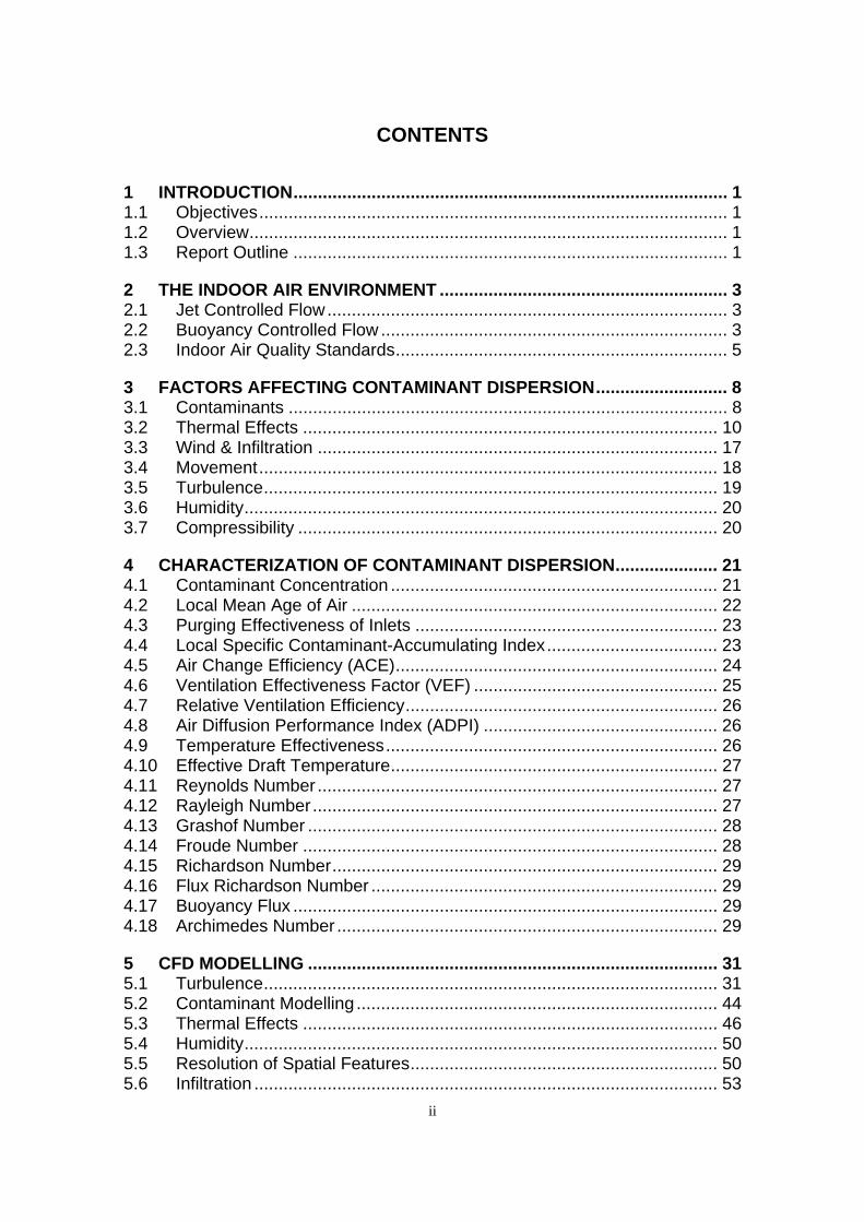
1.2 OVERVIEW To help summarize the information provided in this report, the main factors affecting indoor contaminant dispersion are identified on the schematic of Figure 1. Primary factors that are clearly important in controlling the contaminant transport around the room include the contaminant properties and room ventilation. Secondary factors which perhaps may not seem initially so important include solar radiation, humidity and heat transfer through the walls, floor and ceiling. These secondary factors can have a significant influence on the air flow around the room which, in turn, affects contaminant dispersion. More details, including cross-references to the relevant sections of the report, are provided in Table 1.

1.3 REPORT OUTLINE The report starts with a brief introduction to different types of indoor air flow and the standards which relate to indoor air quality. Following this, the main factors influencing contaminant dispersion are presented, including properties of contaminants, thermal effects such as buoyancy and radiation, turbulence and humidity. A number of parameters which are used to characterize indoor air flows are then presented. These parameters provide guidance on whether certain flow features are significant in a given situation, for example on whether a flow is laminar or turbulent, or whether buoyancy effects are significant. The final section discusses particular modelling issues for the use of Computational Fluid Dynamics (CFD), such as resolution of objects or people, simplifications to buoyancy treatments and turbulence modelling issues.

2

Figure 1 Schematic of the main factors influencing contaminant dispersion

Table 1 Summary of factors affecting contaminant dispersion cross-referenced to the relevant Section number

Physical Room Feature Factors Affecting Contaminant Dispersion

Doors

Door opening (§3.4.3), pumping effect (§3.4.4)

Windows & walls

Thermal effects (§3.2), radiation (§3.2.3), infiltration (§3.3)

Occupants Heat output (§3.2.4, §5.3.3), movement (§3.2.6, §3.4.2), breathing (§3.4.1), flow blocking effects (§5.5.3), spatial resolution (§5.5.2)

Equipment, lights & Furnishings

Heat output (§3.2.5), flow blocking effects (§5.5.3)

Air flow Turbulence (§3.5, §5.1), humidity (§3.6, §5.4), compressibility (§3.7), supply terminals (§5.5.1)

Contaminants Physical properties (§3.1.1, §3.1.2), electrostatic charge (§3.1.3), source location (§3.1.4), contaminant models (§5.2)

Solar radiation

Supply air conditions: velocity, temperature, humidity, contaminant concentrations, turbulence intensity, location

Air flow: turbulence, buoyancy

Exhaust: location, flow rate

Air infiltration through open windows or cracks

Equipment & lights: heat, contaminant sources

Heat transfer through walls, ceiling and floor

Furniture: flow blocking effect, porosity

Doors: air leakage, pumping effect from opening

Occupants: sensible & latent heat gains, contaminant source, movement, humidity

Contaminant: source location, properties (density, phase etc.)

3

2 THE INDOOR AIR ENVIRONMENT

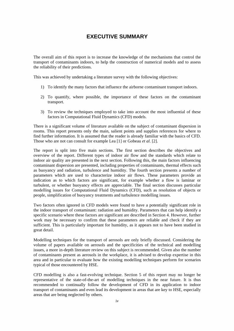
There are many different ways in which the distribution of air inside rooms can be classified. Examples of some possible flow patterns are shown in Figure 2. The following general classification into jet (or momentum) controlled flows and buoyancy controlled flows is proposed by Etheridge & Sandberg [5] and Linden [6]. This classification covers both forced and naturally-ventilated spaces.

Figure 2 Examples of general room air distribution methods (Reprinted from Goodfellow & Tähti [7] with permission from Elsevier). From left to right, they classify

the four rooms as: piston, stratification, zoning and mixing ventilation.

2.1 JET CONTROLLED FLOW In jet-controlled flow, air is introduced into the space using high-velocity devices. The jets of air cause enhanced mixing and dilution of contaminants. When cool air is supplied from high-level devices such as ceiling-mounted diffusers or grilles, the air speed in the occupied zone is generally higher than when the room is supplied with the same inlet flow rate under isothermal conditions. When buoyancy forces are sufficiently strong (i.e. when the temperature difference between supply and room air is sufficiently large), the cold jet separates from the ceiling and falls into the occupied zone. The point at which this separation occurs is controlled primarily by the location of heat sources within the room. Whether the jet separates from the ceiling or not is characterized by a critical discharge Archimedes number, Ardis. This expresses the ratio of buoyant forces to momentum forces (see Section 4 for details). In the case where warm air is supplied at high level, there is a risk that the jet will not penetrate fully into the space. To ensure that there is sufficient penetration, Ardis must be maintained below a critical value, i.e. it must have sufficient momentum for a given supply/room temperature difference.

2.2 BUOYANCY CONTROLLED FLOW In buoyancy-controlled indoor environments the air motion is controlled by heat sources in the room and fresh air is usually supplied at relatively low-velocity. Four supply/extract configurations can be considered:

• Air supply at low level and extract at high level (displacement ventilation)

4

• A single opening at high level • A single opening at low level • A single side opening

With cool air supplied at low level into a room and extracted at high level (a configuration known as displacement ventilation), stable stratification leads to warm air floating above colder, denser air. The room can be simplified into two zones, a lower zone where air movements are predominantly in the horizontal direction towards heat sources and an upper zone that contains regions of flow recirculation (see Figure 3). In such cases, the contaminant concentration does not usually increase linearly with height. Instead, concentrations are fairly uniformly low in the lower part of the room, high in the upper part and between these two zones the concentration increases sharply (see Figure 4). Under typical room conditions this transitionary layer between the upper and lower zones is around 0.5 metres thick [6]. The height of the transitional layer above the floor decreases if either the extent of the buoyant plume(s) increases or if more heat is extracted through the walls of the room.

Figure 3 Schematic view of a room with displacement ventilation

Linden [6] presents a simple model that predicts the height of the transitional layer based on empirical correlations involving the effective area of the room openings, number of sources and height difference between openings. The model predicts a reduction in the height of the transitional layer by approximately a factor of 2 when the buoyancy source is redistributed from a single flux into 10 equal sources, due to enhanced entrainment. The two-layer structure of displacement ventilation breaks down in regions where the flow is moving vertically: in plumes, close to supply devices and near walls where heat transfer occurs. In terms of occupant exposure to contaminants, one advantage of displacement ventilation compared to jet-controlled flow is that air quality in the occupied space can be at the supply condition, whereas in jet-controlled ventilation fully-mixed conditions are more likely to be encountered [8]. This is, however, dependent upon the temperature stratification, the location of contaminant sources and the location of thermal plumes created by heat sources (e.g. occupants, lamps). Displacement ventilation is only applied in rooms where a constant supply of cooling air is required to offset heating loads in the space. The minimum temperature of the supply air is limited by the thermal discomfort experienced by occupants due to the temperature gradient from floor to ceiling level.

5

Figure 4 Contaminant and temperature profiles in a test room with displacement ventilation. The heat source is vertical pillar in the centre of the room from floor to

ceiling and contaminant is released at the foot of the cylinder (reproduced with permission from Heiselberg & Sandberg [9])

A single opening at high level for both supply and extract leads to mixed conditions in the room. The cool air descending from the opening interacts with buoyant plumes rising in the room leading to fairly uniform temperatures. In contrast, a single low-level opening causes stable stratification throughout and is not, generally, an efficient way to ventilate spaces. Single-sided ventilation is probably the most common form of natural ventilation in domestic premises. Horizontal temperature gradients are sometimes generated which drive gravity currents. Considerable discussion of this, and the effect of wind forces, is given in Linden [6].

Linden presents the concept of a ‘neutral level’, where the pressures inside and outside the building are equal. Above the neutral level, pressure inside the building is greater than outside and flow is from inside to outside. Below the neutral level the reverse is true (air flows from outside to the room interior). This clearly has implications for the location of smoke ventilation openings.

For details of generic room configurations, such as hospital operating theatres or standard offices, see the CIBSE and ASHRAE guides [10, 11]. These provide data on air change rates and typical heat gains in the space.

2.3 INDOOR AIR QUALITY STANDARDS

ASHRAE Standard 62 defines acceptable indoor air quality as air in which there are no known contaminants at harmful concentrations and where the substantial majority of people (80% or more) do not express dissatisfaction. The definition covers occupant comfort, odours and harmful levels of contaminants.

Examples of common contaminants include: carbon dioxide, carbon monoxide, micro-organisms, viruses, allergens and suspended particulate material. These contaminants are introduced into indoor spaces by human and animal occupancy, by the release of contaminants

6

in the space from furnishings, accessories and/or processes taking place in the space, or from the supply of contaminated fresh air. Poor indoor air quality may be discernible by occupants as visible suspended particulate matter in the air or odours, or may be discernible only by sensitive measuring devices.

In the UK, the primary regulation governing occupational exposure to harmful substances is the Control Of Substances Hazardous to Health (COSHH) regulations. This presents eight measures which employers or employees must take to maintain safe working practices. These include tasks such as risk assessment, control measures, monitoring and training. Exposure limits are specified in the HSE publication EH40/2005: Workplace Exposure Limits. Failure to comply with the COSHH regulations can result in prosecution.

In addition to these regulations, the design of indoor environments has been affected by targets on energy efficiency in buildings. The UK is committed to reducing its carbon emissions by 20% by the year 2010, based on 1990 levels. This is being encouraged by the government Energy Efficient Best Programme and the Climate Change Levy [10]. Part L of the Building Regulations in England and Wales is currently being revised to set stringent conditions on energy use. Amongst other controls, the measures aim to minimize energy losses due to air leakage through gaps in the fabric of buildings. In response to concerns that there should be adequate ventilation to maintain good indoor air quality, Part F (Ventilation) of the Building Regulations is also being revised.

Below is a summary of sources of information on contaminants, safe occupational exposure levels, recommended practices and regulations:

• HSE

o COSHH Regulations: Approved Code of Practice and Guidance1 o COSHH Essentials: Easy Steps to Control Chemicals2 o EH40/2005: Workplace Exposure Limits o Advisory Committee on Dangerous Pathogens publications3

• UK Building Regulations4

o Part D: Toxic Substances (for insulation materials) o Part F: Ventilation o Part J: Combustion Appliances and Fuel Storage Systems o Part L: Conservation of Fuel and Power

• UK Health Protection Agency5

• UK Department for Environment, Food and Rural Affairs (DEFRA)6

• Committee on the Medical Effects of Air Pollutants (COMEAP) – part of the UK

Department of Health7 • CIBSE

o Guide B2: Ventilation and Air Conditioning 1 http://www.hse.gov.uk/coshh 2 http://www.coshh-essentials.org.uk 3 http://www.hse.gov.uk/aboutus/meetings/acdp/index.htm 4 http://www.odpm.gov.uk/stellent/groups/odpm_buildreg/documents/sectionhomepage/odpm_buildreg_page.hcsp 5 http://www.hpa.org.uk/ 6 http://www.defra.gov.uk/environment/airquality/index.htm 7 http://www.advisorybodies.doh.gov.uk/comeap/index.htm

7

• European Directives8

o Framework Directive 96/62/EC (outdoor air quality) o Daughter Directive 1999/30/EC

• ASHRAE

o HVAC Applications Chapter 45: Control of Gaseous Indoor Air Contaminants o Fundamentals Chapters 9: Indoor Environmental Health o Fundamentals Chapter 12: Air Contaminants.

• U.S. Occupational Safety & Health Administration (OSHA) • U.S. Environment Protection Agency (EPA) 9

8 http://europa.eu.int/comm/environment/air/ 9 http://www.epa.gov/air/

8

3 FACTORS AFFECTING CONTAMINANT DISPERSION

This section discusses the main factors that control the airborne transport of contaminants around a room. The manner in which contaminants interact with room air is dependent upon the contaminant properties: whether it is lighter or heavier than air, gaseous or particulate etc. These properties are addressed in the first section. Following this are descriptions of thermal effects (i.e. buoyancy currents), wind and infiltration, movement of people, doors and windows, turbulence, humidity and compressibility.

3.1 CONTAMINANTS

3.1.1 Common Contaminants

Here the discussion centres on common contaminants in typical home or work environments. Considerable detail is presented in ASHRAE Fundamentals Chapter 12: Air Contaminants (see also [12]). For measured data on contaminants in school environments, see Carrer et al. [13]. A review of possible sources of contaminants and occupational exposure target levels is given in Goodfellow & Tähti [7].

• Carbon Dioxide – exhaled as a by-product of all mammalian metabolism and typically found in higher concentrations in occupied spaces. It is a measurable indicator of the ventilation efficiency and is often used as an indirect indicator of levels of other potentially harmful gases. The EPA recommends maximum CO2 levels of 1000 ppm (1.8 g/m3) for continuous exposure.

A sedentary person takes between 15 and 40 breaths per minute with each breath replacing about 1 litre of air [5]. Exhaled air contains about 4% CO2 [14] compared to around 0.03 % found in the earth’s atmosphere. Human CO2 production rates depend on the activity level: active pre-school children produce around 12 l/hr, sedentary office workers 18 l/hr and light industrial or domestic workers 36 l/hr [15].

• Carbon Monoxide – generated by tobacco smoking and incomplete combustion of hydrocarbons. Sources include improperly ventilated heating or cooking appliances. Buildings with air intakes close to garages, loading docks or at low level in congested streets can draw high levels of CO into occupied spaces10. It is a toxic gas and levels near 15 ppm can significantly affect body chemistry.

• Sulphur Oxides – produced by combustion of hydrocarbon fuels containing sulphur. It can be introduced into rooms via air intakes or from leaks with combustion systems inside the building. Hydrolysed with water, sulphur oxides form sulphuric acid which can irritate moist mucus membranes and parts of the upper respiratory tract. It may also lead to asthma attacks.

• Nitrous Oxides – caused by high-temperature combustion of hydrocarbons. NOx can be introduced into the space by poorly positioned ventilation inlets near internal combustion engines and industrial plant.

• Radon – a naturally occurring gas caused by the radioactive decay of uranium and thorium present in rocks. The primary concern is as a cause of lung cancer. Radon is

10 Design of such intakes and the relevant standards are described in ASHRAE HVAC Applications, Chapter 44: Building Air Intake and Exhaust Design.

9

now recognized to be the second largest cause of lung cancer in the UK after smoking. It can enter buildings from the soil, through cracks in slab floors, basement walls, through the water supply and from building materials containing traces of radioactive elements. Exposure levels are minimized by pressurizing spaces (to minimize ingress), by ventilation and through sealing cracks in the floor. In the UK, workplaces found to contain radon concentrations in excess of 400 Bequerels per cubic metre must comply with the Ionising Radiations Regulations, 1999 (IRR99).

• Volatile Organic Compounds (VOC’s) – typical modern indoor environments have a large number of potential sources of organic (carbon-containing) chemical species: from combustion sources, pesticides, building materials and finishes, cleaning agents and solvents, plants and animals. Formaldehyde is a particularly common irritant and is used in the manufacture of carpets, insulation, textiles, paper products, cosmetics and phenolic plastics. These products off-gas formaldehyde over long periods of time, though largely over the first year after manufacture. Maximum occupational exposure levels for a number of different VOC’s are specified in the HSE document: Workplace Exposure Limits (EH40/2005). Recent research on the ‘sorption’ (i.e. binding of one material to another) of VOC’s to building materials has been sponsored by ASHRAE11. Further information on sorption of VOC’s is available in ASHRAE Fundamentals Chapter 22: Sorbents and Desiccants.

• Particulate Matter (PM) – this refers to suspended solid or liquid matter in air and includes a wide range of particle sizes from 0.01 – 100 µm. ASHRAE classifies PM according to size and type (solid/liquid/complex), covering: dusts, fumes, smokes, mists, fogs, smogs and bioaerosols. Examples of small particulates include viruses and tobacco smoke, while large particulates include dust mites, pollen and saw dust. The size of particles has a marked effect on their deposition efficiencies in the nasal and tracheo-bronchial passages and in the lungs. Atmospheric particles are composed mainly of two size ranges, fine particles (approximately 0.1 - 1 µm) and coarse particles (5 - 50 µm). Each range has its own set of physical and chemical properties. Some particles are volatile, appearing either in vapour or solid phase depending on the ambient temperature, relative humidity or vapour concentration. The EPA and the EU have both developed health standards for occupant exposure to particulates (PM2.5 and PM10 standards). Health effects of particulate exposure include: difficulty breathing, asthma, bronchitis, silicosis and asbestosis. Textile materials, such as carpets and curtains, can act as indoor reservoirs for particulates (particularly mites, proteins and allergens).

3.1.2 Contaminant Properties

Due to the large range of possible contaminants, it is not possible to list all of their properties here. Instead, information can be found from the following references:

• ASHRAE Fundamentals, Chapter 12: Air Contaminants • AirLiquide: gas data online12 • Thermodynamic tables

11 ‘A Critical Review on Studies of Volatile Organic Compound (VOC) Sorption by Building Materials’, ASHRAE RP-1097 and 4508 and ‘Effects of Environmental Conditions on the Sorption of VOC’s on Building Materials’, ASHRAE RP-1097 and 4578 (see http://tc410.ashraetcs.org/content.html for details). 12 http://www.airliquide.com/en/business/products/gases/gasdata

10

• Fluid dynamics textbooks and HVAC design guides, e.g. [7, 16, 17] • Commercial CFD packages

Some contaminants are affected by changes in local flow conditions, for instance ammonia production in chicken litter is sensitive to local temperature and humidity. Zhang & Haghighat [18] investigated how the rate of material emissions vary as a function of the local air velocity flowing over a surface.

3.1.3 Electrostatically Charged Particles The UK Health Protection Agency recently investigated13 corona discharges from overhead power lines and their effect on electrostatically charging airborne pollutants. Results showed that for particles larger than about 0.3 µm, the particle charge was unlikely to have a significant effect on deposition in the lungs, but for smaller particles, around 0.1 µm in diameter, there was up to a three-fold increase in deposition. The HPA work concluded that contaminant particles charged electrostatically from power lines were unlikely to have more than a small effect on long-term health. There is a considerable amount of material available in the literature regarding electrostatic air filters (precipitators or charged-media filters) and room air ionisers. The latter devices work by electrostatically charging particles suspended in room air which are then attracted to walls, floors, table tops, occupants, etc. Information on these devices, how they operate and their potential as sources of ozone can be found in Goodfellow & Tähti [7] and from the US EPA website14.

3.1.4 Location of Contaminant Sources The location of contaminant sources can have a significant effect on occupational exposure. Etheridge & Sandberg [5] discuss the experiments of Stymme et al. [19] where contaminant concentrations were measured in a room with displacement ventilation. The sources of contaminant were positioned either close to the ceiling, the floor, near one of the occupants or near the stratification layer. Results showed that contaminants released below the stratification layer, either near the floor or low down on a wall, tended to accumulate below the stratification layer and were gradually convected horizontally towards heat sources. Once at the heat sources, contaminants were entrained into the buoyant plume and transported vertically upwards. If the contaminants were released directly into the upper stratified zone, the buoyant plume surrounding occupants brought fresh air from near the floor level so that contaminant concentrations in the breathing zone were relatively low.

3.2 THERMAL EFFECTS

As discussed in Section 2, the flow pattern in a room with displacement ventilation is primarily controlled by thermal sources. To model the contaminant dispersion behaviour in these rooms accurately, it is critical that heat transfer and buoyancy are accounted for appropriately. 13 http://www.hpa.org.uk/radiation/publications/documents_of_nrpb/abstracts/absd15-1.htm 14 http://www.epa.gov/iaq/pubs/residair.html

11

There is a significant amount of information on room heat loads in HVAC design guides such as CIBSE and ASHRAE, and building services engineering text books such as McQuiston & Parker [12]. The main heat sources or sinks in rooms include the following:

• Transmission of heat by conduction through solid surfaces: walls, ceiling and floors. • Radiation between solid surfaces within the room • Solar radiation through glazing • Sensible and latent heat gains from occupants • Heat gains from equipment, e.g. computers, lights • Infiltration or air leakage

In the following sections, the three fundamental mechanisms of heat transfer are presented: conduction, convection and radiation. Following this, the heat gains in a typical room due to occupants and equipment are described. Finally there is a discussion of transient thermal effects and the implication for modelling air flows in rooms. Infiltration is covered later in Section 3.3.

3.2.1 Conduction

Conduction involves the transmission of heat by collisions between molecules or atoms but does not involve any mass transfer. The equation governing one-dimensional conduction is Fourier’s law:

xTqx ∂

∂−= λ

where qx is the heat flux in the x-direction per unit area (in W/m2), λ the thermal conductivity and ØT/Øx the temperature gradient in the x-direction. Values of λ for air can be found in the Thermodynamic Tables or in heat transfer textbooks (e.g. [17]).

3.2.2 Convection

Convection involves a moving fluid (gas or liquid), and is often associated with heat transfer from a fluid to a solid or vice versa. The actual transfer of heat from the solid particles to those of the fluid occurs by conduction but heat is then rapidly transported away due to the fluid motion. Convection is classified as natural, forced or mixed. In natural convection, the motion of the fluid is driven solely by buoyancy due to changes in density of the fluid. Forced convection is driven by pressure differences or fluid momentum that is induced by, for example, a fan or a pump. Mixed convection is a combination of the two.

The flow behaviour at the fluid-solid interface controls the rate of convective heat transfer. In a laminar boundary layer there is little mixing and flow is usually parallel to the wall. Heat transfer therefore takes place mainly by conduction. Turbulent boundary layers involve significant mixing of the near-wall fluid with the outer stream and heat transfer rates are significantly larger (see also Section 3.5: Turbulence).

To understand the relative importance of conduction and convection, Tennekes & Lumley [20] present a simple order-of-magnitude analysis for a typical room with a radiator against one wall. If there is no air motion in the room and heat is transferred solely by conduction, they calculate that it takes around 100 hours for heat to diffuse across the room. For the same flow, but now

12

accounting for buoyancy-driven convection currents, they calculate the equivalent time scale to be around 2 minutes. Clearly, heat transfer by convection is rapid compared to that by pure conduction.

3.2.3 Radiation Radiation is the transmission of energy by electromagnetic waves or photons. Unlike conduction and convection there does not have to be a carrier medium (gas/liquid/solid) in order to transmit radiative energy.

3.2.3.1 Emission of Radiation The amount of radiation a body emits is a function of the material properties and the absolute temperature of the emitter. This is expressed by:

4TW εσ=

where W is the total energy emitted per unit time and unit area, ε is the hemispherical emittance, σ is the Stefan-Boltzmann constant (σ = 5.670 × 10-8 W/m2⋅K4) and T is the absolute temperature in Kelvin. For a perfect black-body emitter, ε is unity. Emissivities for common materials are tabulated in ASHRAE Fundamentals. For typical wall interiors made of white or light cream brick, tile, the emissivity is between 0.85 and 0.95.

Thermal radiation takes place over a range of wavelengths, typically 0.1 < λ < 100 µm (predominantly infra-red). The magnitude of the radiation varies with wavelength. As the temperature of a black body emitter increases, so the wavelength of the emitted radiation becomes shorter.

3.2.3.2 Incident Radiation When radiative energy falls on a surface it can be reflected, absorbed or transmitted through the material. This can be expressed as:

1=++ ρτα where: α fraction of incident radiation absorbed (absorptance) τ fraction of incident radiation transmitted (transmittance) ρ fraction of incident radiation reflected (reflectance) For opaque materials (i.e. most solids) the transmittance is zero, τ = 0, and for black bodies all the energy is absorbed, i.e. α = 1 and ρ = τ = 0. Kirchoff’s Law states that the absorptance and emittance of bodies are equal for a given wavelength and direction:

θλθλ εα ,, =

13

If the radiation or the surface are ‘diffuse’, the absorptance and emittance at a given wavelength are the same in all directions. Furthermore, if the bodies are black or ‘gray’15 and at the same temperature, the wavelengths of the radiation are the same and therefore:

εα = For most materials the absorptance of solar radiation is different to the emittance at normal room temperatures, since the wavelength distributions are different (the sun with a surface temperature of around 6000 K and a wall at, say, 295 K). For typical wall interiors made of white or light cream bricks or tiles, the absorptance of solar radiation is between 0.3 and 0.5. Most calculations of thermal radiation assume that surfaces are black or ‘gray’16. Other assumptions commonly made include:

• Radiation is diffuse. • Properties are uniform over the surfaces • The fluid between the surfaces neither emits nor absorbs radiation, i.e. has τ = 1.

Whilst these assumptions greatly simplify the problem, the results should be seen as approximate.

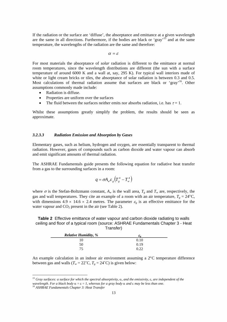
3.2.3.3 Radiation Emission and Absorption by Gases Elementary gases, such as helium, hydrogen and oxygen, are essentially transparent to thermal radiation. However, gases of compounds such as carbon dioxide and water vapour can absorb and emit significant amounts of thermal radiation. The ASHRAE Fundamentals guide presents the following equation for radiative heat transfer from a gas to the surrounding surfaces in a room:

( )44wggw TTAq −= εσ

where σ is the Stefan-Boltzmann constant, Aw is the wall area, Tg and Tw are, respectively, the gas and wall temperatures. They cite an example of a room with an air temperature, Tg = 24°C, with dimensions 4.9 × 14.6 × 2.4 metres. The parameter εg is an effective emittance for the water vapour and CO2 present in the air (see Table 2).

Table 2 Effective emittance of water vapour and carbon dioxide radiating to walls ceiling and floor of a typical room (source: ASHRAE Fundamentals Chapter 3 - Heat

Transfer) Relative Humidity, % εg

10 0.10 50 0.19 75 0.22

An example calculation in an indoor air environment assuming a 2°C temperature difference between gas and walls (Tw = 22˚C, Tg = 24˚C) is given below:

15 Gray surfaces: a surface for which the spectral absorptivity, α, and the emissivity, ε, are independent of the wavelength. For a black body α = ε = 1, whereas for a gray body α and ε may be less than one. 16 ASHRAE Fundamentals Chapter 3: Heat Transfer

14

( ) ( ) ( ) ( )448 15.29515.29719.024.26.1424.29.426.149.41067.5 −⋅⋅××+××+××⋅×= −q

which gives: q = 529 W. Compared to heat gains in the space of around 100W from a single occupant, the emission of radiation from the air with a ∆T of 2°C is significant. For large furnaces, thermal radiation from gas to walls is the dominant mode of heat transfer. Absorptance of thermal radiation by air is governed by Beer’s Law which states that the attenuation of radiant energy in a gas is a function of PgL, the product of the partial gas pressure and the path length. The absorptance varies according to the spectral content of the radiation and the temperature, pressure and composition of the gas. Details of this calculation are not provided in ASHRAE fundamentals. The online Inframet guide (http://www.inframet.pl) also discusses absorption of radiation in the atmosphere for applications of thermal imaging, but does not provide details of any calculation method.

3.2.3.4 Solar Radiation

There are three main factors influencing the amount of solar radiation striking part of the earth’s surface:

• The distance between the sun and the earth. This changes through the year due to the elliptic orbit of the earth. As a consequence, the earth receives about 7 percent more total radiation in January than in July.

• The tilt of the earth on its axis at 23.5° with respect to the orbital plane. From March 21 to September 22/23 (the vernal and autumnal equinoxes) the northern hemisphere is subject to greater solar radiation than the southern hemisphere and vice versa.

• The rotation of the earth on its axis. The earth rotates through one 360° revolution every 24 hours (i.e. in one hour the earth rotates through 15°).

The amount of incident radiation can be found from the location on the earth’s surface, the time of day, and the day of the year. For details of how to find the angle of the sun from the horizontal and vertical at a given location and given time, see McQuiston & Parker [12].

The solar radiation reaching the earth’s surface is composed of two parts: direct radiation from the sun and diffuse radiation that includes radiation scattered or re-emitted by clouds, gas and dust particles in the atmosphere. The value of the incident radiation (in terms of W/m2) can be calculated using the ASHRAE ‘Clear Sky Model’ – see McQuiston & Parker again for details.

3.2.3.5 Magnitude of Radiation Compared to Conduction and Convection Etheridge & Sandberg [5] have suggested that modelling radiation in indoor air environments is necessary to obtain the correct temperature profiles. They discussed the experimental work of Heiselberg & Sandberg [9], which involved a heated column in the middle of a rectangular test room with tracer gas injected at the base of the column, low-level air inlet and high-level extract. The temperature increased fairly uniformly with height from the floor whereas contaminant profiles exhibited a shallow gradient both near the floor and near the ceiling, with a much steeper gradient in between (see Figure 4 on page 5). They explain the difference between the temperature and contaminant profiles as being due to the transport mechanisms for heat and

15

contaminant being different. Both are transported by convection and diffusion, but heat is also transported by a third process, radiation. Howell & Potts [21] compared experimental measurements of displacement ventilation in an enclosure with numerical simulations either with or without a radiation model. They found that results from the numerical simulations were in poor agreement with experiments when radiation was ignored, but results obtained with the radiation model were in good experimental agreement. Ongoing work at HSL has shown that radiation modelling can be important in certain flows. In a study of a single occupant standing in the centre of the room with displacement ventilation, CFD results were closer to the experimental temperature and contaminant concentrations with a radiation model rather than without. In the particular case studied, air velocities throughout most of the room were very low and the flow was dominated by buoyancy due to heat transfer from the occupant. There was little change in the CFD predictions from assuming the air to be either transparent (ε = 0.01) or with a realistic emissivity (ε = 0.17). In contrast, other in-house studies of a seated occupant in a room in which velocities were generally higher showed little or no effect from using a radiation model. One explanation for this difference in behaviour is that when flows are primarily buoyancy-driven, small differences in the surface temperatures due to radiative heat transfer may have significant effects on the flow velocity. In momentum-driven flows, small differences in temperature have only a secondary effect on the flow. In theory it might be possible to classify whether a radiation model should or should not be necessary according to a local Richardson number or similar parameter. However, to our knowledge, no such criteria have been developed.

Howell & Potts [21] also discussed the salt-bath technique that is used experimentally to simulate displacement ventilation. This technique uses density stratification of salt in water to mimic the stratification of air in rooms. They noted that the salt-bath technique does not account for thermal radiation, and significantly underestimates thermal diffusion (the diffusivity of salt in water is less than one ten-thousandth that of heat in air). Their experiments using air as the flow medium showed significant differences to those obtained previously using salt-baths. They concluded that simple numerical models of displacement ventilation that have been validated using salt-bath experimental data are unlikely to capture important physical heat transfer mechanisms that take place in real-life situations.

3.2.4 Heat Gains from Occupants The heat released by people is often tabulated in design guides in terms of sensible and latent heat loads17. Table 3 gives details of the sensible and latent heat loads for a man undertaking various activities. Heat loads for females and children are typically 85% and 75% of the male values respectively. ‘Low Velocity’ and ‘High Velocity’ in Table 3 refer to the local air velocity around the person. When the air velocity is higher, a greater proportion of the sensible heat loss is through convection rather than radiation, hence the values in the ‘Low Velocity’ column are all higher than for ‘High Velocity’. A slightly different breakdown of heat gains from people is given by Etheridge & Sandberg [5], see Table 4.

17 The two relevant chapters in ASHRAE Fundamentals are Chapter 8 - Thermal Comfort and Chapter 29 - Nonresidential Cooling and Heating Load Calculation Procedures.

16

Table 3 Heat loads for different activity levels and the proportion of heat lost due to radiation (from ASHRAE Fundamentals Chapter 29 Table 1)

Activity % Sensible Heat that is Radiant

Total Heat, W

Sensible Heat, W

Latent Heat, W Low Velocity High Velocity

Seated, very light office work

130 70 45 60 27

Light bench work in a factory

295 110 185 49 35

Athletics in a gymnasium

585 210 315 54 19

Sensible energy is related to the kinetic energy of the molecules and is proportional to the temperature of the fluid. The rate of sensible heat transfer to a fluid, qs, to raise the temperature of the fluid which is flowing at a mass flow rate m& by ∆T Kelvin is calculated from:

Tcmq ps ∆= & where cp is the specific heat capacity of the fluid at constant pressure. Latent energy is related to the phase-change process between liquids and gases. In a humidifying process the rate at which heat needs to be added, ql, to vaporize liquid at a mass flow rate, m& , is given by:

miq fgl &= where ifg is the enthalpy of vaporization. Most numerical simulations of air flows in rooms do not account for latent heat transfer (see also Section 3.6: Humidity).

Table 4 Approximate heat losses from people (source: Etheridge & Sandberg [1])

Mode of Heat Loss Percentage (%) Radiation 40 Convection 40 Insensible water loss by breath 10 Insensible water loss by skin 10

3.2.5 Heat Gains from Equipment Heat gains from light fittings and other equipment are covered in ASHRAE Fundamentals Chapter 29 – Nonresidential Cooling and Heating Load Calculation Procedures. The heat gains from lights are divided into two parts: a heat-to-space part which goes directly into the occupied zone, and a heat-to-return part which will be transferred into a ceiling void if there is a false ceiling in the room. Tables of heat output are provided for various lighting fixtures.

17

For office equipment such as computers, printers and monitors, the nameplate data on the equipment itself does not give an accurate value for the actual heat output. Generally, for office equipment with a power output of less than 1 kW, a conservative guide for the heat output is 50% of the nameplate value, whilst a more accurate figure may be 25%. There is, however, significant variability in these figures. Tables of recommended heat gains for many types of equipment including those commonly found in offices, hospitals and catering establishments are presented in the ASHRAE guide.

3.2.6 Transient Thermal Effects

In real-life situations, the air flow pattern in rooms is unlikely to be statistically steady. Heat loads rarely stay constant over time. Over a day and throughout the year the outside air temperatures change, solar gains increase and decrease, occupants come and go and there are thermal inertia effects from the building fabric. A steady-state solution based on given outside temperature and solar radiation conditions may therefore differ from a snapshot of the transient calculation.

Linden [6] discusses the scenario of an auditoria suddenly filling up with people and the transient warm-up phase of the space. As the auditoria fills, warm air generated by the occupants rises as a plume and forms a stratified layer, which gradually descends as a displacement ventilation flow pattern is established. Experiments and theoretical analysis show that the interface between the warm/cool air descends below the ultimate steady-state level (i.e. it overshoots). The amount of overshoot is a function of the floor space surface area and the time taken to reach steady state conditions. For a 500-seat lecture theatre, the timescale for the establishment of steady state conditions was estimated as being about one hour, i.e. steady-state conditions are rarely fully established. This overshoot behaviour was also observed in the recent work of Kaye & Hunt [22].

Transient effects are discussed in terms of the time-delay effect of thermal loads in Chapter 29 of ASHRAE Fundamentals. See also the section on dynamic simulation of thermal buildings in Goodfellow & Tähti [7].

3.3 WIND & INFILTRATION

Practically all structures leak air to some extent, allowing infiltration into or out of indoor spaces via small cracks around windows, walls and doors. This leakage can have considerable effect on heat loss calculations in cold climates. Considerable guidance on calculating leakage rates is therefore given in HVAC design guides, particularly those from the U.S. (e.g. McQuiston & Parker [12]). Flow patterns in occupied spaces are likely to be affected by air ingress through cracks, particularly if the air leaking into the space is at a different temperature (peak winter/summer conditions) or at a high velocity, due to strong wind pressures on the building exterior. Air leakage into spaces can also carry pollutants from the exterior environment. Infiltration is covered in Chapter 26 of the ASHRAE Fundamentals guide. Simple expressions for how one can sum the pressure differences due to wind, mechanical ventilation and stack effect (i.e. density differences due to temperature imbalance) are presented. Experimental data is referenced, together with tables showing the range of leakage rates to be expected from various building elements: windows, doors, fireplaces etc. Two ASHRAE Standards are also relevant:

18

Standard 136 provides procedures for calculating infiltration rates in detached dwellings and Standard 119 gives performance specifications infiltration for residential housing. Modern building standards are aimed at reducing infiltration so that building heat loads are minimized, see the UK Building Regulations for details18.

3.4 MOVEMENT

3.4.1 Breathing Considerable detail is given in Goodfellow & Tähti [7] on the human respiratory tract, including breathing mechanics, intra-airway airflow patterns, and heat and water vapour transport within the airways. Data for exhaled air volumes based on the 1996 Health Survey for England are presented. Typical volume flow rates are 6-8 l/min. Curves are provided showing how the flow rate changes over a single breath. Reynolds numbers are also examined: the air flow through nasal passages is turbulent, even in normal quiet breathing, whilst flow further down in the pulmonary airways it is generally laminar.

3.4.2 Movement of people Mattsson & Sandberg [23] studied experimentally a moving manikin in a displacement ventilated room. Contaminant concentrations at head height were found to increase with the velocity of manikin, rising eventually to levels higher than the ambient conditions at the same height above the floor. This was due to the entrainment of contaminated air from the upper part of the room into the wake of the manikin and the disruption of the boundary layer around the body which prevented clean air from below reaching head height.

3.4.3 Door opening A study of the exchange of air from one room to another as a person walks through the doorway linking the two rooms entraining air in his/her wake was presented in Etheridge & Sandberg [5]. For a door of typical dimensions (90 × 205 cm), the exchange volumes were between 0.087 and 0.29 m3 depending on the speed of the walk19.

Etheridge & Sandberg [5] also discuss the transient motion of air between rooms of different temperature when a door leading from one room to the other is opened. They present equations for the velocity and flow rate based on Bernoulli-type assumptions of frictionless flow.

3.4.4 Door swing pumping Kiel & Watson [24] measured the volume of air displaced either side of a door when it was opened and closed. Under isothermal and non-isothermal conditions using a 1:20 scale model, they found that for a 90º opening and shutting of the door there was a linear relationship

18 http://www.odpm.gov.uk/stellent/groups/odpm_buildreg/documents/sectionhomepage/odpm_buildreg_page.hcsp 19 It is not clear in the text whether this is experimental or numerical simulation. Since the work was undertaken in the 1970’s it is likely to be experimental.

19

between the pumped volume, Vp, (measured in m3) and the mean door speed, ud (in m/s measured at the door centre), given by:

dp uV 3.2= where the pumped volume equates to around 50% of the volume swept by the door.

3.5 TURBULENCE Fluid flow can be classified into three regimes: laminar, transitional and turbulent. In fully laminar flow, streamlines appear smooth and without any significant fluctuations. As the characteristic Reynolds number of the flow increases, small fluctuations become amplified, the flow becomes less stable and eventually undergoes transition to turbulence. In fully-turbulent flow, the motion is disordered, seemingly random and there is greater mixing. A classic example of laminar, transitional and turbulent flow is shown in Figure 5. Laminar flow tends only to occur at low speed, with viscous fluids and in constricted spaces. The majority of flows relevant to contaminant dispersion are mixed laminar/turbulent or fully-turbulent. Turbulence intensities in a typical rooms have been measured to be around 30%, with much of the turbulence energy composed of frequencies less than 2 Hz [5]. Rates of heat transfer and mixing due to turbulence are several orders of magnitude larger than those due to molecular diffusion. This is illustrated by the example in Section 3.2.2 on convective heat transfer. In addition to having a significant impact on contaminant dispersion, the magnitude of turbulent velocity fluctuations affects occupant comfort. ASHRAE Standard 55-92 presents guidelines for the allowable local air speed in the occupied zone as a function of air temperature and turbulence intensity.

Figure 5 Three photos showing laminar, transitional and turbulent flow of dye in a

water-filled pipe, respectively, from top to bottom (reproduced with permission of the Mechanical, Aerospace and Civil Engineering School, University of Manchester, UK)

20

3.6 HUMIDITY

In most temperate climates, humidity is not seen as a particular issue for indoor comfort. In particularly cold climates, however, where the outdoor air can be very dry, fresh air may be humidified before being supplied to the occupied space. This is achieved by introducing water vapour or by spraying fine droplets of water into the air stream.

At 20ºC, the relative molecular mass of dry air is 28.97 whilst for saturated air it is 28.71 (the wet air is actually less dense as the relative molecular mass of water is only 18.015). This difference in air density between relative humidity 0% and 100% is the same as that found by raising the temperature of dry air from 20 to 22.6ºC. One would expect significant differences in humidity to cause measurable buoyancy effects.

Gradients of airborne water vapour in a room are likely to be significant if there is a cold surface on which moisture is condensing out of the air or if there are sources of high humidity, such as steam-generating equipment. Exhaled air from human breathing has high humidity levels, typically around 80-90%. Humidity can be an important factor controlling the release of other contaminants. Nimmermark and Gustafsson [25] studied a room used by laying hens and measured emissions of odour, ammonia, carbon dioxide and dust concentration. Both odour and ammonia emissions were found to increase significantly with water vapour pressure20. High humidity inside buildings is also related to prevalence of mould allergens, fungi and bacteria [13]. At low humidity there is a reduction in the electrical conductivity of clothing, carpets and soils, which may affect deposition of charged particulate contaminants. Humidity also has an effect on thermal radiation, changing the absorptance, transmittance and emittance properties of air (see Table 2 on page 13).

3.7 COMPRESSIBILITY The ASHRAE Fundamentals guide states that compressibility effects, such as shock waves, are relevant when the Mach number exceeds 0.2. At room temperature and sea level, this equates to: 0.2 × 343 = 69 m/s. Air supply velocities in rooms are unlikely to ever exceed even 10 m/s (21 mph) and therefore compressibility effects are unlikely to have a significant impact on indoor air flow.

20 Water vapour pressure, Pv, is related to humidity, ω, as follows:

v

v

a

v

PPP

mm

−==

622.0ω

where mv and ma are the masses of water vapour and dry air present in the mixture and P is the total static pressure.

21

4 CHARACTERIZATION OF CONTAMINANT DISPERSION

In this section, a number of parameters are used to characterize the dispersion of a contaminant inside a room. Table 5 lists these parameters and groups them under four headings: fresh air or contaminant distribution, temperature distribution, stability and buoyancy of the room air, and supply air conditions. Due to overlap between these subjects, some parameters appear more than once. Some parameters characterize directly the observed pattern of contaminant distribution whilst others characterize flow features, such as stability.

Flow parameters such as the ‘mean age of air’ are difficult but not impossible to calculate experimentally. They are used mainly as a tool to help interpret data from numerical simulations of contaminant dispersion. For discussions on how these parameters are used to assess compliance with standards on room air quality, see Peng & Davidson [8] or the ASHRAE Guides [11].

Table 5 Summary of parameters which characterize contaminant dispersion in rooms Fresh Air/ Contaminant Distribution

• Contaminant Concentration (p21) • Local Mean Age of Air (p22) • Purging Effectiveness of Inlets (p23) • Local Specific Contaminant-

Accumulating Index (p23) • Air Change Efficiency (p24) • Ventilation Effectiveness Factor (p25) • Relative Ventilation Efficiency (p26)

Stability and Buoyancy of the Room Air • Reynolds Number (p27) • Rayleigh Number (p27) • Grashof Number (p28) • Froude Number (p28) • Richardson Number (p29) • Flux Richardson Number (p29) • Buoyancy Flux (p29)

Temperature Distribution • Air Diffusion Performance Index (p26) • Temperature Effectiveness (p26) • Effective Draft Temperature (p27)

Supply Air Conditions • Purging Effectiveness of Inlet (p23) • Reynolds Number (p27) • Froude Number (p28) • Archimedes Number (p29)

4.1 CONTAMINANT CONCENTRATION Clearly the simplest indicator of contaminant distribution in a room is the contaminant concentration, i.e. the mass of contaminant per unit volume of air (measured in kg/m3). Alternative units for contaminant concentration include:

• Molar concentration: the number of moles of contaminant per unit volume of mixture. • Mass fraction: the mass of contaminant divided by the mass of the mixture. • Mole fraction: the ratio of the number of moles of contaminant to the number of moles

of the mixture. For mixtures of ideal gases, the mole fraction and the volume fraction are equivalent.

Contaminant concentration is sometimes expressed in terms of parts per million (ppm), or parts per billion, trillion etc. This can be based on either the mass fraction or the volume fraction. Perhaps because of this ambiguity, the U.S. National Institute of Standards and Technology

22

(NIST) guide for the use of the International System of Units (SI), states that “the language-dependent terms: part per million, part per billion, and part per trillion ... are not acceptable for use with the SI to express the values of quantities”21. Under fully mixed conditions, the local contaminant concentration, C, is equal to its equilibrium value everywhere:

qmCC e&

==

where m& is the mass flow rate of contaminant and q the volume flow rate of air.

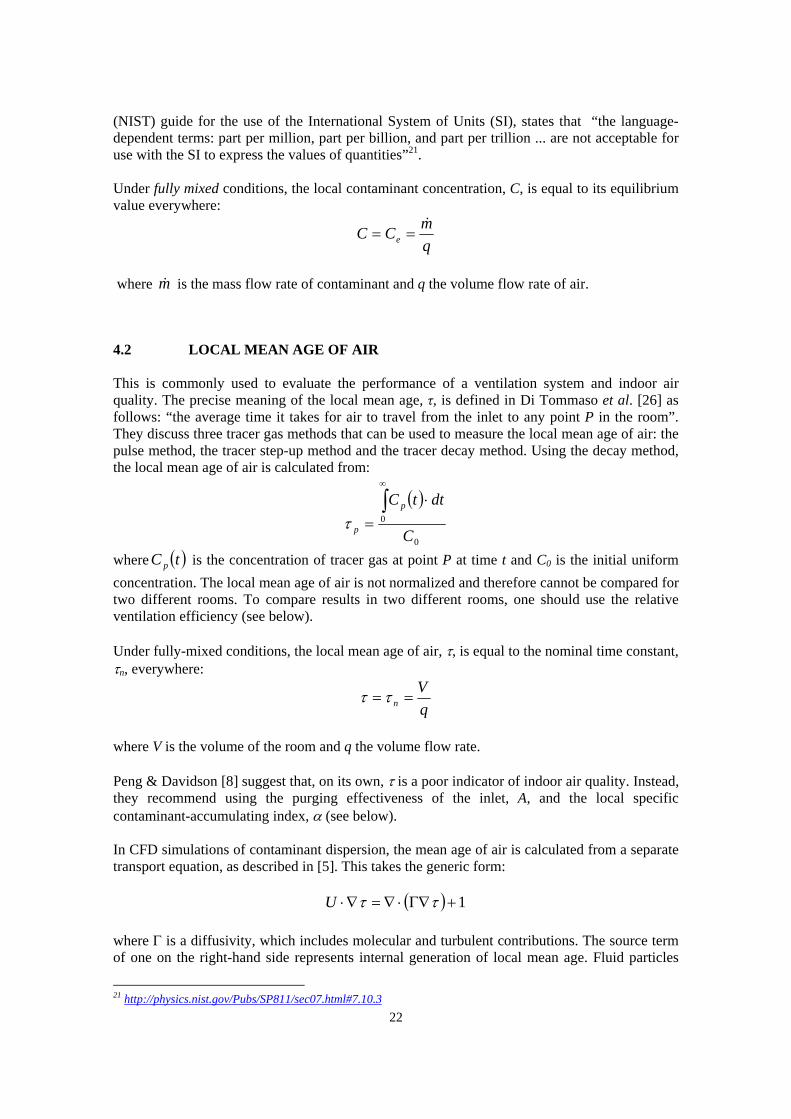
4.2 LOCAL MEAN AGE OF AIR This is commonly used to evaluate the performance of a ventilation system and indoor air quality. The precise meaning of the local mean age, τ, is defined in Di Tommaso et al. [26] as follows: “the average time it takes for air to travel from the inlet to any point P in the room”. They discuss three tracer gas methods that can be used to measure the local mean age of air: the pulse method, the tracer step-up method and the tracer decay method. Using the decay method, the local mean age of air is calculated from:

( )

0

0

C

dttC p

p

⋅=

∫∞

τ

where ( )tC p is the concentration of tracer gas at point P at time t and C0 is the initial uniform concentration. The local mean age of air is not normalized and therefore cannot be compared for two different rooms. To compare results in two different rooms, one should use the relative ventilation efficiency (see below). Under fully-mixed conditions, the local mean age of air, τ, is equal to the nominal time constant, τn, everywhere:

qV

n == ττ

where V is the volume of the room and q the volume flow rate. Peng & Davidson [8] suggest that, on its own, τ is a poor indicator of indoor air quality. Instead, they recommend using the purging effectiveness of the inlet, A, and the local specific contaminant-accumulating index, α (see below). In CFD simulations of contaminant dispersion, the mean age of air is calculated from a separate transport equation, as described in [5]. This takes the generic form:

( ) 1+∇Γ⋅∇=∇⋅ ττU

where Γ is a diffusivity, which includes molecular and turbulent contributions. The source term of one on the right-hand side represents internal generation of local mean age. Fluid particles

21 http://physics.nist.gov/Pubs/SP811/sec07.html#7.10.3

23

entering the flow domain are assigned an initial age (usually zero) and the source term increments the age for every second spent inside the domain.

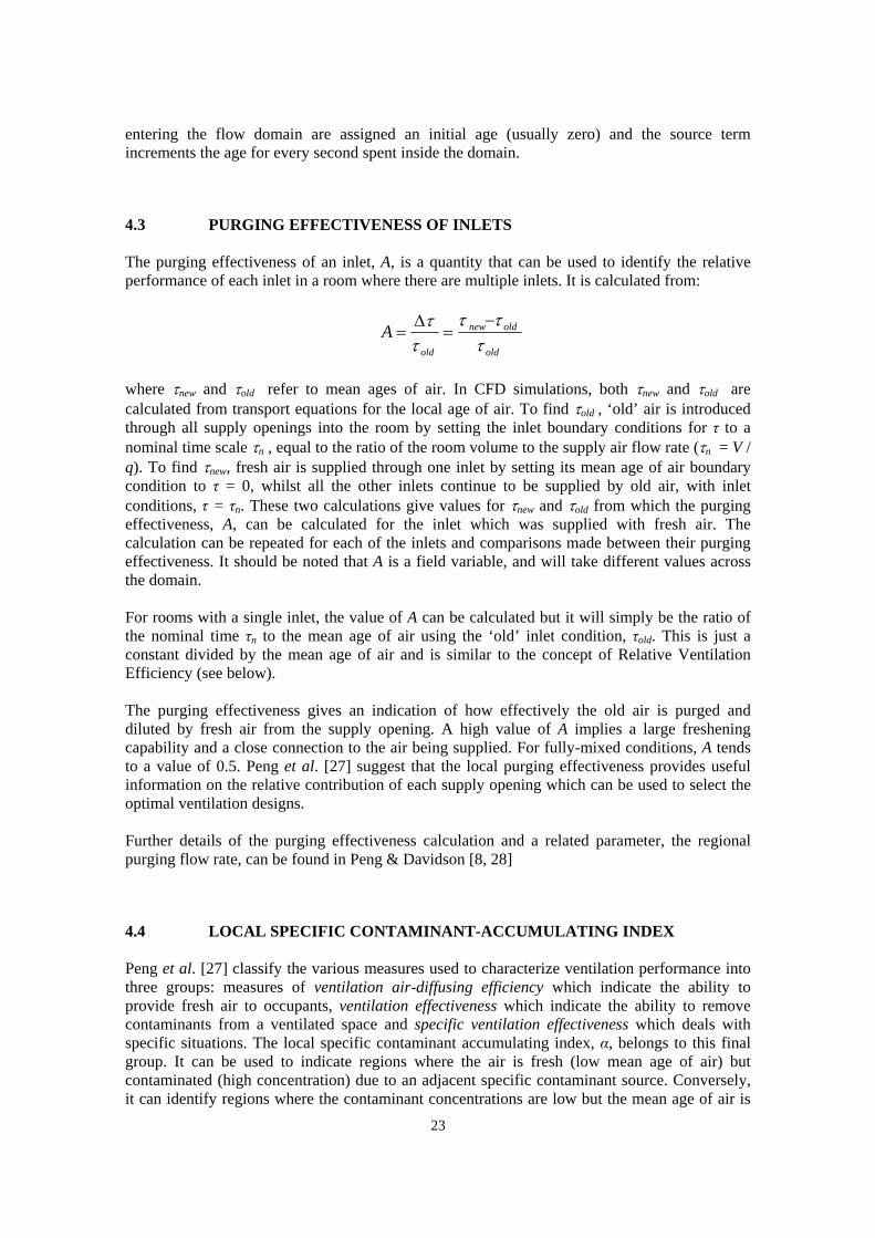
4.3 PURGING EFFECTIVENESS OF INLETS

The purging effectiveness of an inlet, A, is a quantity that can be used to identify the relative performance of each inlet in a room where there are multiple inlets. It is calculated from:

old

oldnew

old

Aτ

τττ

τ −=

∆=

where τnew and τold refer to mean ages of air. In CFD simulations, both τnew and τold are calculated from transport equations for the local age of air. To find τold , ‘old’ air is introduced through all supply openings into the room by setting the inlet boundary conditions for τ to a nominal time scale τn , equal to the ratio of the room volume to the supply air flow rate (τn = V / q). To find τnew, fresh air is supplied through one inlet by setting its mean age of air boundary condition to τ = 0, whilst all the other inlets continue to be supplied by old air, with inlet conditions, τ = τn. These two calculations give values for τnew and τold from which the purging effectiveness, A, can be calculated for the inlet which was supplied with fresh air. The calculation can be repeated for each of the inlets and comparisons made between their purging effectiveness. It should be noted that A is a field variable, and will take different values across the domain. For rooms with a single inlet, the value of A can be calculated but it will simply be the ratio of the nominal time τn to the mean age of air using the ‘old’ inlet condition, τold. This is just a constant divided by the mean age of air and is similar to the concept of Relative Ventilation Efficiency (see below). The purging effectiveness gives an indication of how effectively the old air is purged and diluted by fresh air from the supply opening. A high value of A implies a large freshening capability and a close connection to the air being supplied. For fully-mixed conditions, A tends to a value of 0.5. Peng et al. [27] suggest that the local purging effectiveness provides useful information on the relative contribution of each supply opening which can be used to select the optimal ventilation designs.

Further details of the purging effectiveness calculation and a related parameter, the regional purging flow rate, can be found in Peng & Davidson [8, 28]

4.4 LOCAL SPECIFIC CONTAMINANT-ACCUMULATING INDEX Peng et al. [27] classify the various measures used to characterize ventilation performance into three groups: measures of ventilation air-diffusing efficiency which indicate the ability to provide fresh air to occupants, ventilation effectiveness which indicate the ability to remove contaminants from a ventilated space and specific ventilation effectiveness which deals with specific situations. The local specific contaminant accumulating index, α, belongs to this final group. It can be used to indicate regions where the air is fresh (low mean age of air) but contaminated (high concentration) due to an adjacent specific contaminant source. Conversely, it can identify regions where the contaminant concentrations are low but the mean age of air is

24

high. It can be thought of as a general index capable of reflecting the interaction between the ventilation flow and a specific contaminant source. The local specific contaminant-accumulating index, α, is calculated from [8]:

⎟⎟⎠

⎞⎜⎜⎝

⎛=

Cnτγα ln

where τn = V/q and C is the mean room concentration. The denominator Cnτ represents

the mean exposure of the whole space to contaminant during one air change. The parameter γ is the local age-integrated exposure which is calculated from:

( )∫ ⋅=τ

γ0

dttC

In the above expression, τ is the local mean age of air which must be determined in advance either from tracer experiments or by solving a transport equation for τ in the CFD model. For a steady-state flow, the local age-integrated exposure is simply τγ C= . Negative values of α indicate a large contaminant diluting capability at that location ( )Cnτγ < . Under well-mixed conditions ( )Cnτγ ≈ the value of α is close to zero.

4.5 AIR CHANGE EFFICIENCY (ACE) This is a measure of how effectively the air present in a room is replaced by fresh air from the ventilation system [26]. It is the ratio of the room mean age that would exist if the air in the room were completely mixed (τn = V/q) to the average time of replacement of the room (τexc):

100⋅=exc

nACEττ

where:

( )

( )∫

∫∞

∞

⋅

⋅⋅⋅=

0

02dttC

dttCt

e

e

excτ

and ( )tCe is the concentration inside the exhaust duct. ACE values are comparable in different rooms, since the value is normalized. A value of 100% indicates piston flow, 50% indicates fully-mixed conditions, and a value less than 50% implies that there is short-circuiting. Di Tommaso et al. [26] developed correlations between the air change efficiency (ACE) and the inlet Archimedes number (Ar) for mixing ventilation in rooms with different wall and inlet temperatures. An increase in the absolute value of Ar led to an increase in ACE when the supply air was warmer than the walls, and to a decrease in ACE when the supply air was cooler than the walls. The behaviour is likely to be sensitive to the room configuration and should not be considered generally valid. In their study, the rooms considered had low-level inlet and high-level extract. For more details of the ACE calculation, see Sandberg & Sjoberg [29].

25

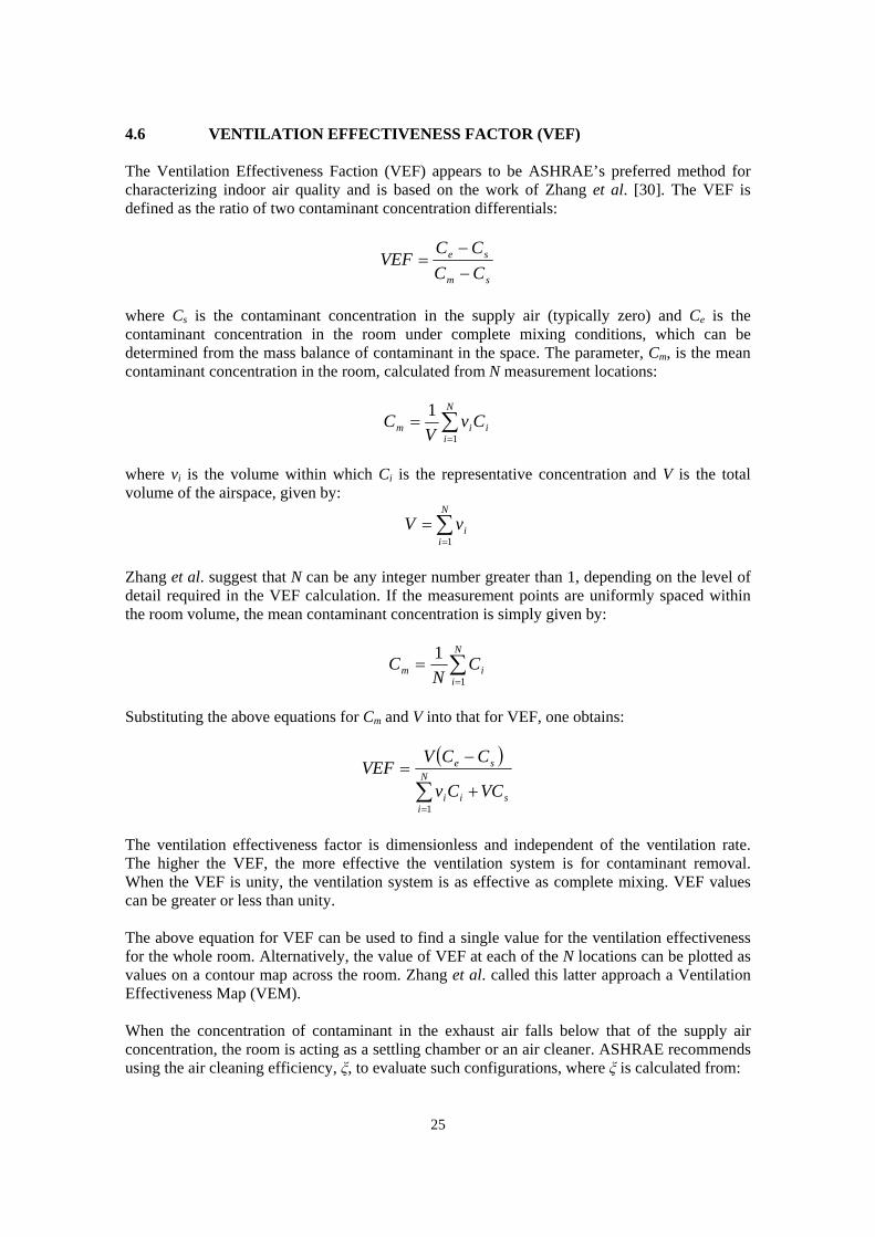
4.6 VENTILATION EFFECTIVENESS FACTOR (VEF) The Ventilation Effectiveness Faction (VEF) appears to be ASHRAE’s preferred method for characterizing indoor air quality and is based on the work of Zhang et al. [30]. The VEF is defined as the ratio of two contaminant concentration differentials:

sm

se

CCCC

VEF−−

=

where Cs is the contaminant concentration in the supply air (typically zero) and Ce is the contaminant concentration in the room under complete mixing conditions, which can be determined from the mass balance of contaminant in the space. The parameter, Cm, is the mean contaminant concentration in the room, calculated from N measurement locations:

∑=

=N

iiim Cv

VC

1

1

where vi is the volume within which Ci is the representative concentration and V is the total volume of the airspace, given by:

∑=

=N

iivV

1

Zhang et al. suggest that N can be any integer number greater than 1, depending on the level of detail required in the VEF calculation. If the measurement points are uniformly spaced within the room volume, the mean contaminant concentration is simply given by:

∑=

=N

iim C

NC

1

1

Substituting the above equations for Cm and V into that for VEF, one obtains:

( )

s

N

iii

se

VCCv

CCVVEF

+

−=

∑=1

The ventilation effectiveness factor is dimensionless and independent of the ventilation rate. The higher the VEF, the more effective the ventilation system is for contaminant removal. When the VEF is unity, the ventilation system is as effective as complete mixing. VEF values can be greater or less than unity. The above equation for VEF can be used to find a single value for the ventilation effectiveness for the whole room. Alternatively, the value of VEF at each of the N locations can be plotted as values on a contour map across the room. Zhang et al. called this latter approach a Ventilation Effectiveness Map (VEM). When the concentration of contaminant in the exhaust air falls below that of the supply air concentration, the room is acting as a settling chamber or an air cleaner. ASHRAE recommends using the air cleaning efficiency, ξ, to evaluate such configurations, where ξ is calculated from:

26

s

ex

CC

−= 1ξ

The parameter, Cex, in the above equation is the contaminant concentration in the exhaust air.

4.7 RELATIVE VENTILATION EFFICIENCY The relative ventilation efficiency is the ratio of the local mean age that would exist if the air in the room were completely mixed (τn = V/q) to the local mean age that is actually measured at a point (τp).

p

np τ

τε =

Its value gives a measure of spatial variations of air distribution in a room. Since it is normalized with respect to τn, values obtained in different rooms can be compared (unlike the local mean age of air) [26].

4.8 AIR DIFFUSION PERFORMANCE INDEX (ADPI) The ADPI is primarily a measure of occupant comfort rather than an indicator of contaminant concentrations. It expresses the percentage of locations in an occupied zone that meet air movement and temperature specifications for comfort. Details of the calculation method can be found in ASHRAE Fundamentals Chapter 31 – Space Air Diffusion, and in McQuiston & Parker [12]. The ADPI is based only on air velocity and the effective draft temperature (a combination of local temperature variations from the room average). Measurement techniques for assessing a room’s ADPI are specified in ASHRAE Standards 55 and 113, for heating and cooling conditions, respectively.

4.9 TEMPERATURE EFFECTIVENESS The temperature effectiveness is similar in concept to ventilation effectiveness and reflects the ability of a ventilation system to remove heat. It is calculated from:

[ ]%100×−−

=os

esT TT

TTε

where Ts is the supply temperature, Te the extract and

oT the average room temperature. A

small temperature difference between the supply air and average room temperatures, for a given temperature difference between inlet and outlet indicate that the supplied energy is used well ( %100>Tε ). If, on the other hand, there is a short circuit between inlet and outlet, there will be a large difference in temperature between supply and average room temperatures, inlet and outlet temperatures will be similar and the effectiveness will be low ( %100<Tε )

27

4.10 EFFECTIVE DRAFT TEMPERATURE The effective draft temperature, θ, indicates the feeling of coolness due to air motion:

( ) ( )15.08 −−−= xcx VTTθ where Tx and Tc are the local air-stream and average room dry-bulb temperatures (in ºC or K), Vx is the local airstream centreline velocity (in m/s) and θ is measured in K. A high percentage of people are comfortable in sedentary (office-type) occupations when the effective draft temperature, θ, is between –1.5 and +1 K. For further details, see ASHRAE Fundamentals Chapter 32: Space Air Diffusion.

4.11 REYNOLDS NUMBER The Reynolds number, Re, expresses the ratio of the inertial forces to viscous forces:

νULRe ==

forcesviscousforces inertial

where U and L are characteristic velocity and length scales of the flow and ν is the kinematic viscosity. Inertial forces are responsible for destabilizing fluid flows whilst viscous forces damp instabilities. At low Re, flows are laminar and at high Re flows are turbulent. The actual value of Re at which transition from laminar to turbulent flow takes place is flow-dependent. Laminar pipe flow becomes turbulent at approximately Re l 2000 whilst zero pressure-gradient boundary layers become unstable at Reδ l 600 (based on the free-stream velocity and displacement thickness) [20].

4.12 RAYLEIGH NUMBER Natural convection flows are often characterized using the Rayleigh Number, Ra, given by:

ναβ 3TLgRa ∆

=

where g is the acceleration due to gravity (g = 9.81 m/s2), β the coefficient of thermal expansion (where for an ideal gas, β = T1 ), ∆T the temperature difference, L the length scale (e.g. the height of the heated surface), υ the kinematic viscosity and α the thermal diffusivity (α = k / ρCp). The Rayleigh number is related to the likelihood of instabilities leading to chaotic motion. For Rayleigh-Bérnard convection, instability occurs at Ra > 1700 with a fixed upper surface, or Ra > 1100 with an upper free surface22.

22 Source: http://scienceworld.wolfram.com

28

For a plume generated by a heat source of strength q (in Watts), the Rayleigh number is:

kqLgRa

ναβ 2

=

where, in this case, L is the distance from the source and k is the thermal conductivity. For plume flow, a Rayleigh number of Ra > 1010 leads to instability [5].

4.13 GRASHOF NUMBER

The Grashof number, Gr, is equivalent to the Rayleigh number divided by the Prandtl number:

2

3

Pr νβ TLgRaGr ∆

=≡

where g is the acceleration due to gravity, β the coefficient of thermal expansion ∆T temperature difference, L the length scale and υ the kinematic viscosity.

For details of the physical meaning of the Prandtl number, see Section 5.3.1. The Grashof number can also be written based on a heat flux per unit area, q (in W/m2):

2

4

νβk

qLgGr =

where k is the thermal conductivity. Flow over an isothermal wall is laminar up to Gr < 1.5 × 109 whereas for constant wall heat flux the flow is laminar up to Gr < 1.6 × 1010 [5].

4.14 FROUDE NUMBER

The following form of the Froude number is used by Linden [6] to characterize flow through corridors and doorways and in combined displacement and wind ventilation cases.

gLUFr

2

=

where U and L are characteristic velocity and length scales, respectively, and g the acceleration due to gravity. Goodfellow & Tähti [7] use a slightly different form of the equation to describe the location at which a non-isothermal jet penetrating into a room changes from momentum-controlled to buoyancy-controlled mode, i.e. from a jet to plume:

( )∞

∞

−=

TTT

gDU

Fr00

20

29

where U is the velocity, D the inlet diameter and T the temperature. Subscript ‘0’ refers to the inlet condition and ‘∞’ the far field. This relationship between the buoyancy forces and momentum flux is also characterized by the Archimedes number, Ar (see Section 4.18).

4.15 RICHARDSON NUMBER The Richardson number, Ri, characterizes the importance of buoyancy. It is calculated from:

ρρ∆

= 2UgLRi

where ∆ρ is the density difference that occurs over a typical (usually vertical) length scale, L, in a flow of velocity, U. The buoyancy tends to zero as Ri → 0. The Richardson number implies that buoyancy effects are significant if there is either significant density differences (large ∆ρ/ρ) as occurs for example in plumes, or if the ratio gL/ρU2 is significant, as occurs in the atmospheric boundary layer [17].

4.16 FLUX RICHARDSON NUMBER The flux Richardson number, Rif, is used to characterize the stabilizing effect of stratification on turbulence:

k

kbf P

PRi −=

where Pkb and Pk are the turbulence production due to buoyancy and shear respectively (see Section 5.1 on turbulence modelling). If the buoyancy production is positive, Rif < 0 and turbulent kinetic energy is increased. Conversely, for positive Rif, turbulence is damped. Experiments have shown that turbulence cannot be sustained for Rif ≥ 2 (Durbin & Pettersson Reif [31]).

4.17 BUOYANCY FLUX The buoyancy flux, B, is calculated from:

pcWgB

ρβ

=

Linden [6] uses this to characterise buoyancy driven flows, where W is the heat flux, T1=β

is the coefficient of expansion and cp is the specific heat capacity at constant pressure.

4.18 ARCHIMEDES NUMBER

30

The conditions of the supplied air are often characterised by the discharge Archimedes number, Ar, which expresses the ratio of the buoyancy forces to momentum forces or the strength of natural convection to forced convection:

TT

UAgAr ∆

= 2

where T∆ is the temperature difference between supply and exhaust, U is the initial velocity of the discharged air, g is the acceleration due to gravity and L is the length scale of the supply terminal (i.e. diffuser or grille). High Ar indicates that buoyancy forces are strong so that, for instance, a downward directed jet is likely to reverse flow sooner than for low discharge Ar. The Archimedes number is sometimes used to characterize the distance travelled by a ceiling jet of cool air before it detaches and descends into the room. Di Tommaso et al. [26] define the Archimedes number as:

TUgLAr ∆= β2

where β is the volume expansion coefficient, L is a characteristic length (e.g. inlet height) and U the air velocity (e.g. average inlet velocity). The discharge Archimedes number is the inverse of the Froude number presented in Section 4.14.

31

5 CFD MODELLING

Previous sections have discussed the main factors controlling contaminant dispersion in rooms and identified characteristic parameters that describe the flow phenomena. The following section discusses the simulation of contaminant dispersion using Computational Fluid Dynamics (CFD).

CFD is not the only technique that can be used to simulate contaminant transport in rooms. Etheridge & Sandberg [5] present a number of simplified analytical models which calculate contaminant concentrations based on the source location, mass transfer coefficient, geometry of source, velocity of emission and time history. There are also simple models based on the zonal approach [32]. The advantage of CFD over these alternative treatments is its generality: it can provide reasonably accurate results for a range of different flows and relies less upon case-specific empiricism. That is not to say that CFD always gives good results. Part of the aim of the discussion below is to provide guidance on the accuracy of different sub-models and to give practical advice on how best to simulate a contaminant dispersion problem.

It should be noted that whilst CFD offers advantages in terms of accuracy and generality, it can also be significantly more expensive than the simple modelling approaches in terms of computing time. To assess the dispersion of a contaminant over large distances and over long physical time periods (many hours or days) simple models may be the only practical approach available.

The discussion below has been limited to consideration of the physical models. For information on numerical methods, including differencing schemes and convergence criteria, see for example Sørensen & Nielsen [33].

5.1 TURBULENCE

Computers are not yet sufficiently powerful to be able to directly resolve all of the fine eddy structures in industrial turbulent flows. Projections of future capabilities based on Moore’s Law for the exponential growth of computing power have suggested that the so-called ‘Direct Numerical Simulation’ approach will only become a practical engineering tool in around 2070. At present, two approaches are instead commonly used to model the effect of turbulence on the mean flow behaviour: Reynolds-Averaged Navier-Stokes (RANS) models and Large-Eddy-Simulation (LES). A summary of the RANS and LES models used by the three commercial CFD packages currently used at HSL is presented in Table 6. The accuracy of the turbulence models and their computational cost generally increase moving progressively further down the table. Brief descriptions of RANS and LES models are given below (Sections 5.1.1 to 5.1.5). The accuracy of turbulence models varies depending upon the particular flow features being simulated. The main flow phenomena that are encountered in contaminant dispersion cases are presented in subsequent sections. This includes a discussion of laminar-turbulent transition, jet impingement, 3D wall jets, rectangular ducts, vortex shedding and free jets. Model performance in buoyant flows is considered in Section 5.3.

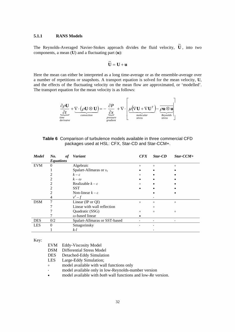
32

5.1.1 RANS Models The Reynolds-Averaged Navier-Stokes approach divides the fluid velocity, U~ , into two components, a mean (U) and a fluctuating part (u):

uUU +=~

Here the mean can either be interpreted as a long time-average or as the ensemble-average over a number of repetitions or snapshots. A transport equation is solved for the mean velocity, U, and the effects of the fluctuating velocity on the mean flow are approximated, or ‘modelled’. The transport equation for the mean velocity is as follows:

{( )

{( )

⎥⎥⎥

⎦

⎤

⎢⎢⎢

⎣

⎡

⊗−∇+∇⋅∇+∂∂

−=⊗⋅∇+∂

∂32144 344 214434421

stressReynolds

stressmolecular

T

gradientpressure

convection

derivatvetime

xP

tuuUUUUU ρµρρ

Table 6 Comparison of turbulence models available in three commercial CFD packages used at HSL: CFX, Star-CD and Star-CCM+.

Model No. of

Equations Variant CFX Star-CD Star-CCM+

0 Algebraic ) ) ) 1 Spalart-Allmaras or υt * * * 2 k – ε ) * * 2 k – ω * * * 2 Realizable k – ε ) * * 2 SST * * * 2 Non-linear k – ε * *

EVM

4 v2 – f $ 7 Linear (IP or QI) ) ) ) 7 Linear with wall reflection ) 7 Quadratic (SSG) ) ) )

DSM

7 ω-based linear * DES 0/2 Spalart-Allmaras or SST-based $ $ $

0 Smagorinsky $ $ LES 1 k-l $

Key:

EVM Eddy-Viscosity Model DSM Differential Stress Model DES Detached-Eddy Simulation LES Large-Eddy Simulation; ) model available with wall functions only $ model available only in low-Reynolds-number version * model available with both wall functions and low-Re version.

33

The Reynolds stress term, uu ⊗ρ , is introduced by the averaging process. RANS modelling consists of finding an accurate approximation to this term. There are two main approaches:

• Eddy-Viscosity Models (EVM’s): the Reynolds stress is calculated from an eddy (or turbulent) viscosity, µt, in a similar fashion to the molecular viscous stress:

( )T

t UUuu ∇+∇=⊗ µρ

The simplest, linear EVM, shown above, assumes that the stress, uu ⊗ρ , is proportional to the strain-rate, ( )TUU ∇+∇ . Additional transport equations are usually solved for parameters such as the turbulent kinetic energy, k, the dissipation rate, ε, in order to calculate the eddy-viscosity. There are a number of limitations to the accuracy of this simple approach.

• Differential Stress Models (DSM’s): transport equations are solved for each component of the Reynolds stress and for a length-scale parameter, usually ε. In 2D this involves 4 additional equations and, in 3D, seven equations. DSM’s are generally more accurate at predicting flows involving swirl, streamline curvature, rapid changes in the strain rate and secondary flows caused by Reynolds-stress gradients.

In addition to these two classes of models are non-linear eddy-viscosity models (NLEVM’s) and algebraic stress models (ASM’s). These typically involve the solution of two or three equations, such as k, ε and another turbulence transport parameter. They have been developed in response to industry requirements for models that are more accurate than simple, linear EVM’s but less costly than full DSM’s. Instead of making the Reynolds stress just a linear function of the strain-rate, they take the stress proportional to quadratic, cubic or quartic functions of the strain rate or vorticity. Quadratic terms are necessary to predict accurately the correct flow behaviour in non-circular ducts, cubic terms for curvature-induced variations of turbulent shear stress (e.g. rotating pipe flows) and quartic terms for normal-stress anisotropy in primary shear (e.g. 3D turbulent wall jets). Simpler turbulence models also exist. Fluent’s Airpak software, aimed specifically at the HVAC market, uses the following simple zero-equation RANS model:

Vlt ρµ 03874.0=

where V is the local velocity and l the wall distance. The use of V directly in the eddy-viscosity means that the model is not Galilean invariant, i.e. the eddy-viscosity changes under translation of the coordinate axes. For indoor air flows similar to homogeneous shear flow, the model would also incorrectly predict non-constant shear stress since the modelled stress is a function of the velocity rather than the velocity gradients. Despite these shortcomings, Fluent has obtained good results using the Airpak code in validation tests. Some turbulent flows are steady or ‘statistically stationary’. In such flows the mean flow velocity, U, stays constant over time. RANS models are particularly efficient at solving such flows, since they only solve for the mean velocity. In addition, with the RANS approach, it is sometimes possible to simplify the geometry of a problem from three-dimensions to 2D, axisymmetric or even 1D, which can further speed-up calculations.

34

In other turbulent flows where large-scale structures are responsible for most of the turbulent transport, unsteady or time-dependent RANS is used (URANS or T-RANS23). Such flows include vortex shedding from cylinders and unsteady buoyant plumes. In most cases, URANS simply involves adding a time-dependent term into the standard RANS equations and the adoption of a time-discretization scheme in the solution algorithm. For further details on the performance of different RANS models, see Pope [34], Durbin & Pettersson Reif [31] or Launder & Sandham [35].

5.1.2 Large-Eddy Simulation Large-Eddy Simulation (LES) is an alternative approach to RANS in which the large, energy-containing eddies are resolved fully and only the small eddies are approximated or modelled. A computational grid is used that is too coarse to capture all the scales of motion. The small scales that are not resolved by the grid are instead accounted for by an energy-dissipation term in the momentum equations. In practice the equations look very similar to those used by RANS with the mean velocity, U, replaced by a filtered or spatially-averaged velocity, <U>. LES modelling approaches are similar to those used in simple RANS (e.g. algebraic or one-equation eddy-viscosity models). It is sometimes argued that small errors in the model are unimportant since the modelled stress should in any case be small (ideally less than 5% of the resolved stress). The three commercial codes currently used in HSL all have available the Smagorinsky LES model. This is an algebraic eddy-viscosity model, where the subgrid-scale (turbulent) viscosity, νt, is calculated from:

( ) Scst2∆=ν

where ∆ is the filter width, usually taken as twice the cube-root of the local grid cell volume, S is the strain-rate invariant and cs is the Smagorinsky constant. There is no generally-accepted value for cs. In different flows, the best results have been obtained using different values for cs in the range between 0.065 and 0.25. The CFX user manual suggests that a value of cs = 0.1 is a suitable choice for most applications. A more sophisticated class of LES models, the so-called ‘dynamic’ models, automatically calculate the local value of cs using a second filtering process. The results using dynamic models are usually more accurate than those obtained using the standard Smagorinsky model, especially in transitional and wall-bounded flows. None of the commercial CFD codes currently used at HSL have dynamic LES models. Since large eddies are resolved fully in LES, it is necessary to have a time-dependent solution even if the flow is statistically stationary. Also, since the evolution of eddies is fully three-dimensional, the solution has to be three-dimensional. The computational grid often needs to be finer than that used in RANS calculations to resolve the details of the turbulent structures. This is particularly the case near walls. These factors lead to computing times being significantly greater for LES than for RANS.

23 There is no difference in the URANS and T-RANS models, only a difference in terminology.

35

Sørensen & Nielsen [33] comment that LES is expensive and does not improve upon RANS model results for fully-developed turbulent flows. However, they do suggest that it shows some promise in non-developed, low-Reynolds-number turbulent flows. Their paper, published in 2003, suggests that LES will probably be a useful tool for the future, but for practical calculations at present one should use RANS models for simulating indoor air flows.

For more details see Pope [34] or Sagaut [36].

5.1.3 LES Grid Resolution To obtain accurate results, Baggett et al. [37] recommended that the modelled subgrid-scale stress should only account for a negligible fraction of the total Reynolds stress. Under these conditions, only the nearly-isotropic eddies are modelled and any errors due to the LES model should be unimportant. In a review of LES modelling for HSE, WS Atkins proposed a more relaxed condition. They recommended that the ratio of the resolved to the total turbulent kinetic energy should be above 70% for ‘medium’ resolution LES and above 80% for well-resolved [38]. A similar criterion for well-resolved LES was proposed by Pope [34]. These measures provide some guidance that can be used retrospectively to assess whether an LES has been well resolved. For a recent example of the application of this approach, see Kempf et al. [39]. It is useful to have some guidance on the appropriate grid resolution prior to running LES, to avoid having to perform multiple costly simulations on different grids. One suggestion, based on the work of Baggett et al. [37], is to use results from prior RANS simulations to help optimise the grid. Baggett et al. examined two flows, a non-equilibrium boundary layer with strong adverse pressure gradient and a circular jet. They showed that the subgrid stress becomes essentially isotropic as the filter width, x∆ , becomes:

10εLx <∆

where the turbulence dissipation length scale is εε

3qL = and iiuuq =2 . The filter width ( x∆ )

in the above expression can be approximated as twice the cube root of the cell volume, ( ) 3/1V∆ ,

and the trace of the Reynolds stress, iiuu , can be written in terms of the turbulent kinetic

energy, iiuuk21

= . Rearranging the above formula then gives:

( ) ( )10

/222/3

3/1 εkV <∆

or, approximately:

( )10

/2/33/1 εkV <∆

Values of k and ε can be obtained from a previous RANS simulation of the flow. The above formula provides some guidance as to the appropriate grid size for large-eddy simulations. See Addad et al. [40] for an example of its application.

36

To fully-resolve the flow in boundary layers, the dimensionless cell sizes near walls should be ( +∆x , +∆y , +∆z ) < (10, 1, 50) in the spanwise, wall-normal and streamwise directions, respectively. For fully three-dimensional boundary layers without defined streamwise and spanwise directions cell dimensions should be ( +∆x , +∆y , +∆z ) < (10, 1, 10). The LES grid should ideally be fairly uniform and cells should not rapidly increase in size. Mittal & Moin [41] recommended a maximum cell stretching rate of 3% if central differencing is used to avoid spurious oscillations with a wavelength twice the filter-width. For upwind-biased differencing, they suggested that slightly higher stretching-rates could be used.

5.1.4 Hybrid RANS-LES All three commercial CFD codes used by HSL incorporate a hybrid RANS-LES treatment called Detached-Eddy Simulation (DES). This uses RANS to model the flow near the wall and LES for the main part of the flow domain. The aim of the technique is to combine the advantageous features of both LES and RANS: accurate resolution of turbulent structures in the main flow domain using LES, and efficient, accurate prediction of the near-wall flow using RANS. Research is still ongoing in this area and current results indicate that there can be some inaccuracies at the interface between the two layers, due to the inherent differences in the modelling approaches. More information on hybrid treatments can be found in the publications of Professor Lars Davidson24 and Dr. Lionel Temmerman25. The CFD code vendor, CFX, is also in the process of implementing a new RANS model called ‘Scale-Adaptive Simulation’ which decreases the eddy-viscosity under certain conditions so that unsteady flow behaviour is resolved, in a similar manner to hybrid RANS-LES [42].

5.1.5 RANS and LES Wall Treatments There are two main approaches that are used for modelling the near-wall region in turbulent flows:

1. Fully-resolving the near-wall flow 2. Using wall functions

In the first case, a fine grid is needed and the turbulence model has to be tuned to produce the correct damping of the turbulent fluctuations near the solid surface. Such models are termed ‘low-Reynolds-number’ models, where the Reynolds number here refers not to the bulk flow but the turbulence Reynolds number, Ret = νε/2k , near the wall. Typically the computational grid is arranged such that the dimensionless distance from the wall to the nearest node, y+, is less than one. The wall function approach uses empirically derived profiles of velocity, temperature and turbulence parameters to approximate the flow behaviour near the wall. In this case, the near-wall grid can be much coarser, with y+ in the range 30 < y+ < 300. Calculations using wall

24 http://www.tfd.chalmers.se/~lada 25 http://www.ae.ic.ac.uk/research/tfms/temmerman.html

37

functions are typically one or two orders-of-magnitude faster to compute than comparable calculations using the full wall-resolution approach. However, the assumed profiles used in wall functions are only valid for flows close to equilibrium, such as plane channel flows and zero-pressure gradient boundary layers. For more complex flows involving flow impingement, boundary layer separation and buoyancy, wall functions can give erroneous results [33]. These errors are often significantly more visible in the thermal field, in terms of predicted heat transfer rates, than in the hydrodynamic field [43]. The CFX code uses a “scalable” wall function which allows any level of grid-refinement near the wall. It should be noted that despite this, the model still uses empirical log-law profiles for velocity and temperature, which may cause errors in complex flows. For simulations of contaminant dispersion in rooms where the flow is driven by thermal buoyancy due to heat transfer, and complex flow phenomena are present (impingement, boundary layer separation and reattachment) the wall-resolution approach should be used where possible.

5.1.6 Laminar-Turbulent Transition

5.1.6.1 Physical Phenomena There are three principal modes of transition from laminar to turbulent flow [44]:

1. Natural Transition: the flow starts off as laminar, a weak instability occurs in the boundary layer which is then amplified through various stages (Tollmien-Schlichting waves, loop vortices, turbulent spots) until the flow becomes fully turbulent.

2. Bypass Transition: turbulence levels are high in the bulk of the flow domain but the

boundary layer is initially laminar. Turbulence diffuses from the free-stream into the boundary layer. Turbulent spots can appear directly, bypassing the preceding stages of instability.

3. Separated-Flow Transition: the laminar boundary layer separates over an obstacle and

transition occurs either in the free shear layer or as the boundary-layer reattaches to the surface.

The distinction between these modes of transition is important as turbulence models are generally able to predict bypass transition but are less well able to predict natural and separated-flow transition. Transition in indoor air flows takes place predominantly in natural and separated-flow modes. In a room situation, the flow next to a heated wall starts of as laminar near the floor and undergoes natural transition to turbulent flow typically a metre or so higher up the wall [6].

5.1.6.2 Characterizing Transition For a given flow situation it is important to know whether the flow is laminar or turbulent. Table 7 presents criteria necessary for laminar flow for a number of different flow configurations. Details of the dimensionless Reynolds, Grashof and Rayleigh numbers (Re, Gr and Ra) are provided in Section 4.

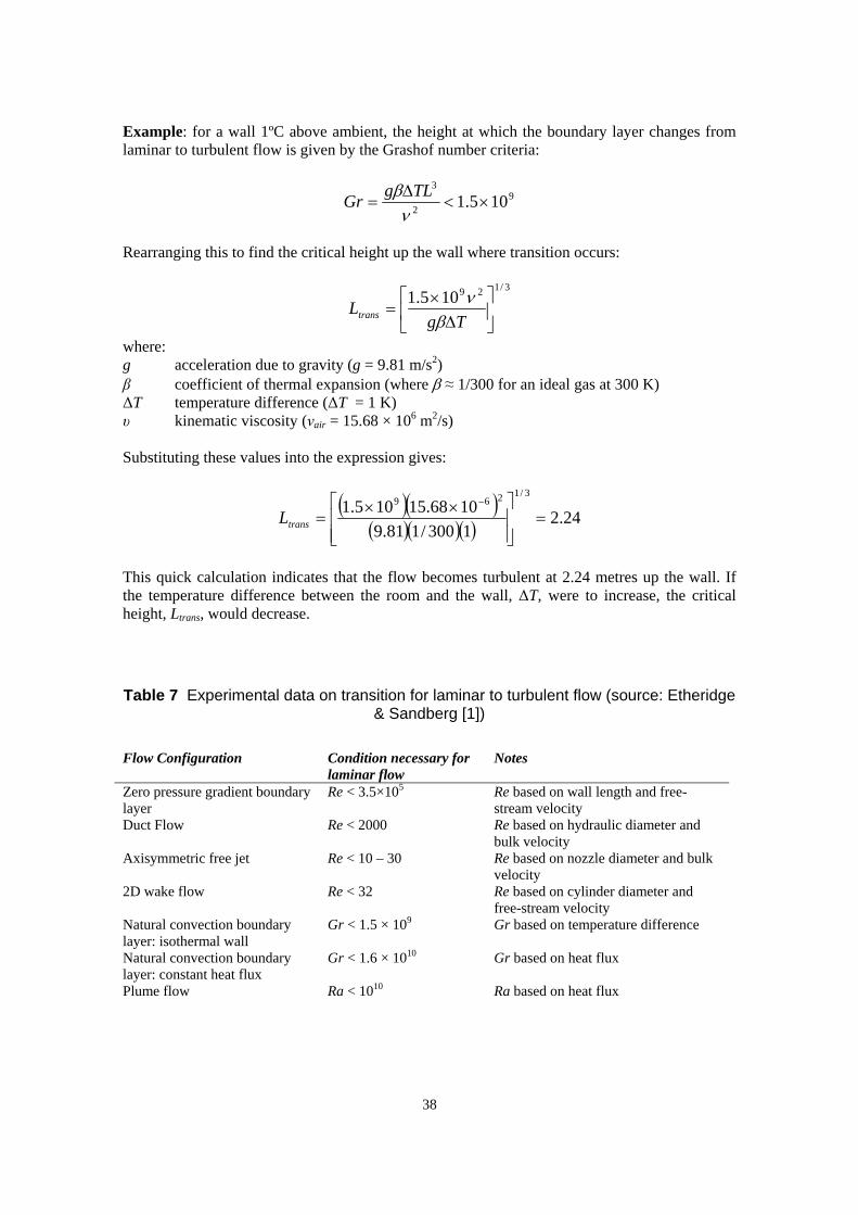
38

Example: for a wall 1ºC above ambient, the height at which the boundary layer changes from laminar to turbulent flow is given by the Grashof number criteria:

92

3

105.1 ×<∆

=ν

β TLgGr

Rearranging this to find the critical height up the wall where transition occurs:

3/129105.1⎥⎦

⎤⎢⎣

⎡∆

×=

TgLtrans β

ν

where: g acceleration due to gravity (g = 9.81 m/s2) β coefficient of thermal expansion (where β ≈ 1/300 for an ideal gas at 300 K) ∆T temperature difference (∆T = 1 K) υ kinematic viscosity (νair = 15.68 × 106 m2/s) Substituting these values into the expression gives:

( )( )( )( )( ) 24.2

1300/181.91068.15105.1

3/1269

=⎥⎥⎦

⎤

⎢⎢⎣

⎡ ××=

−

transL

This quick calculation indicates that the flow becomes turbulent at 2.24 metres up the wall. If the temperature difference between the room and the wall, ∆T, were to increase, the critical height, Ltrans, would decrease.

Table 7 Experimental data on transition for laminar to turbulent flow (source: Etheridge & Sandberg [1])

Flow Configuration Condition necessary for

laminar flow Notes

Zero pressure gradient boundary layer

Re < 3.5×105 Re based on wall length and free-stream velocity

Duct Flow Re < 2000 Re based on hydraulic diameter and bulk velocity

Axisymmetric free jet Re < 10 – 30 Re based on nozzle diameter and bulk velocity

2D wake flow Re < 32 Re based on cylinder diameter and free-stream velocity

Natural convection boundary layer: isothermal wall

Gr < 1.5 × 109 Gr based on temperature difference

Natural convection boundary layer: constant heat flux

Gr < 1.6 × 1010 Gr based on heat flux

Plume flow Ra < 1010 Ra based on heat flux

39

5.1.6.3 Transition Modelling: RANS Natural and separated-flow transition cannot be modelled reliably using RANS schemes. The mechanism of turbulence production in these models relies on the existence of some initial turbulence level. For instance, in the k-ε model, the turbulence production, Pk, is given by:

j

iijtk x

USP

∂∂

= µ

where, using Cartesian tensor notation, Sij is the strain-rate tensor and µt is the eddy-viscosity, which is calculated from:

ερµ µ

2kct =

In a laminar boundary-layer which undergoes transition to turbulence, the turbulent kinetic energy in the upstream, laminar portion of the boundary layer is zero and hence, from the above equation, the eddy-viscosity is zero (µt = 0). To simulate transition, the value of k must increase, but it can only do so if the production term Pk becomes finite. Since the production term depends on µt, and µt is zero, the production term remains zero forever and the boundary layer remains laminar. The only way to avoid this problem in natural and separated-flow transition is to initialise the entire flow field with a finite level of turbulence energy. In areas of the flow where strain-rates are low, turbulence will not be sustained and k-levels will decay gradually to zero as the computation progresses. In other regions, where strain rates are larger, turbulence levels may be sustained. The calculated location of transition found using this approach may not be accurate and tests by the authors have shown that results are sensitive to the local grid resolution. In bypass transition, RANS models may give reasonable predictions. The diffusion of turbulence energy from the free-stream into the boundary layer provides an alternative means of increasing k from the production mechanism outlined above. It is therefore feasible that bypass transition can be predicted. In practice, however, the location of transition is highly model-dependent. A comprehensive, joint-European study of bypass transition was coordinated by Savill [45] in the early 1990’s (see also [46] and [47]). This found that low-Reynolds-number turbulence models employing damping functions based on the turbulence Reynolds number, e.g. the Launder-Sharma k-ε model, performed much better than those based on the distance from the wall. Models using k-ω schemes near the wall, including the SST model, predict transition far too early. CFX have suggested that to model transition, one should use the SST model and manually fix the location of transition by setting a condition based on the momentum thickness Reynolds number, Reθ. This assumes that one has prior knowledge of the transition location. Reverse-transition or laminarization phenomena, where the flow changes from turbulent to laminar (e.g. strongly accelerated boundary layers) can be predicted with good accuracy using traditional RANS closures. In fact, these were some of the first applications of the k-ε model [48].

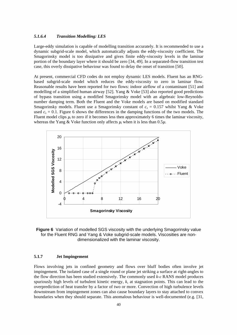
40

5.1.6.4 Transition Modelling: LES Large-eddy simulation is capable of modelling transition accurately. It is recommended to use a dynamic subgrid-scale model, which automatically adjusts the eddy-viscosity coefficient. The Smagorinsky model is too dissipative and gives finite eddy-viscosity levels in the laminar portion of the boundary layer where it should be zero [34, 49]. In a separated-flow transition test case, this overly dissipative behaviour was found to delay the onset of transition [50]. At present, commercial CFD codes do not employ dynamic LES models. Fluent has an RNG-based subgrid-scale model which reduces the eddy-viscosity to zero in laminar flow. Reasonable results have been reported for two flows: indoor airflow of a contaminant [51] and modelling of a simplified human airway [52]. Yang & Voke [53] also reported good predictions of bypass transition using a modified Smagorinsky model with an algebraic low-Reynolds-number damping term. Both the Fluent and the Voke models are based on modified standard Smagorinsky models. Fluent use a Smagorinsky constant of cs = 0.157 whilst Yang & Voke used cs = 0.1. Figure 6 shows the differences in the damping functions of the two models. The Fluent model clips µt to zero if it becomes less then approximately 6 times the laminar viscosity, whereas the Yang & Voke function only affects µt when it is less than 0.5µ.

-4

0

4

8

12

16

20

0 4 8 12 16 20

Smagorinsky Viscosity

Mod

elle

d SG

S Vi

scos

ity

VokeFluent

Figure 6 Variation of modelled SGS viscosity with the underlying Smagorinsky value for the Fluent RNG and Yang & Voke subgrid-scale models. Viscosities are non-

dimensionalized with the laminar viscosity.

5.1.7 Jet Impingement Flows involving jets in confined geometry and flows over bluff bodies often involve jet impingement. The isolated case of a single round or plane jet striking a surface at right-angles to the flow direction has been studied extensively. The commonly used k-ε RANS model produces spuriously high levels of turbulent kinetic energy, k, at stagnation points. This can lead to the overprediction of heat transfer by a factor of two or more. Convection of high turbulence levels downstream from impingement zones can also cause boundary layers to stay attached to convex boundaries when they should separate. This anomalous behaviour is well-documented (e.g. [31,

41

34, 54]). The standard k-ω model suffers from the same problem since it too sets the production of k proportional to the square of the strain-rate. Wall functions reduce somewhat the overproduction of k compared to low-Reynolds-number formulations, although not reliably26. To avoid overproduction of k, several alternatives exist. CFX uses a clip on the magnitude of turbulence production in its version of k-ω model. Both CFX and Star-CD have ‘realizable’ models that make the production proportional to the strain-rate (not the strain-rate squared). Most non-linear eddy-viscosity models and the v2-f model have been tuned to produce the correct behaviour in impinging jets. Differential stress models use the exact production term (i.e. without any modelling approximations) and hence are not subject to the same issues as the eddy-viscosity models. However, the wall-reflection component of the pressure-strain term does affect the models’ performance in impinging flows. For more details, see Craft et al. [55]. LES models appear to be able to predict impinging-jet flow to a good level of accuracy [56, 57], although heat transfer predictions are likely to be affected by the choice of wall boundary conditions: log-law wall functions leading to erroneous predictions near the stagnation point.

5.1.8 3D Turbulent Wall Jets Turbulent wall jets are a feature of indoor air flow near supply air terminals (diffusers and grilles). Prediction of the correct spreading rates of the jet in the wall-normal and wall-parallel directions is especially difficult for RANS turbulence models. Table 8 shows comparisons of standard k-ε, quadratic and quartic non-linear eddy-viscosity models and three differential stress models. There is significant variation in results. Prediction of the correct spreading rates is dependent upon obtaining the correct anisotropy of the Reynolds stresses, which induces axial vorticity. The linear k-ε model incorrectly predicts the spreading rates in wall-parallel and wall-normal directions to be roughly equal. The IP differential stress model with wall reflection terms, which might be expected to provide good predictions of the wall jet, in fact overpredicts the lateral spreading rate by a factor of 2.5. Even the sophisticated TCL and quartic eddy-viscosity models over and under-predict the ratio of lateral to wall-normal spreading rates by a factor of nearly two. The results show that for differential stress models, the wall reflection terms have a significant effect. Nielsen [58] discusses a study which compared the growth of a 3D turbulent wall jet into a long, wide room using k-ε, a differential stress model with wall reflection terms and the v2-f model. The k-ε model incorrectly predicted the spreading rates of the jet to be similar in wall-normal and spanwise directions, whereas the DSM captured the experimentally observed behaviour. The v2-f model was not able to predict the growth rate parallel with the ceiling any better then the k-ε model, despite solving a transport equation for the wall-normal stress. The significance of the 3D wall jet prediction on the overall room air flow is dependent upon the room geometry. Etheridge & Sandberg [5] recommended that one should use a DSM to get the correct room air flow in long, deep rooms dominated by jet-like flow along the ceiling but for more conventional room geometries they stated that there is little difference between using k-ε or a DSM.

26 The assumed log-law profile used by the wall functions is inaccurate near stagnation points, however wall functions assume turbulence conditions close to equilibrium, which keeps the turbulence production closer to experimental values.

42

There does not appear to have yet been any studies of 3D wall jets using LES.

Table 8 Comparison of spreading rates for a 3D turbulent wall jet at Red = 60,000 (taken from Lübcke et al. [47]).

Wall-Normal ( )zy ∂∂ / Wall-Parallel ( )zx ∂∂ / Ratio ( )yx ∂∂ / Experiment 0.065 0.320 4.94 Linear k-ε 0.075 0.061 0.81 Quadratic EVM 0.077 0.065 0.84 Quartic EVM 0.064 0.165 2.57 DSM IP (w/o reflection)

0.081 0.079 0.97

DSM IP (with reflection)

0.053 0.814 15.3

DSM TCL 0.060 0.510 8.54

5.1.9 Rectangular Ducts In rectangular ducts, iso-contours of the axial velocity bulge towards the corners of the duct. This is caused by secondary flow induced by anisotropy of the Reynolds stresses which transports high-velocity fluid from the centre of the duct towards the corners. The magnitude of these secondary velocities is small, at most a few percent of the primary velocity, but the motion has a significant influence on contaminant transport and heat transfer from the walls [59]. Like the 3D wall jet, prediction of the secondary velocities in non-circular ducts is dependent upon obtaining the correct Reynolds-stress behaviour. Linear eddy-viscosity models do not predict any secondary flow patterns at all [60]. Non-linear eddy-viscosity models with quadratic stress-strain dependence are able to capture the correct flow patterns [61]. For differential stress models, it is the rapid part of the linear pressure-strain model that controls the secondary motion. Large-eddy simulation using the standard Smagorinsky model with van Driest near-wall damping has been shown to be able to predict the correct mean velocity profiles in square ducts [62].

5.1.10 Vortex Shedding and Wakes Vortex shedding involves the separation of turbulent eddies from a surface. A commonly cited example is the von Kármán street of alternating vortices formed in the wake of circular cylinders. The flow behaviour downstream of bluff bodies has important implications for contaminant dispersion. Control of occupant exposure by local exhaust ventilation is usually achieved by positioning the sources of contaminant between the person and the extract duct. Experimental and numerical studies by George et al. [63] and Dunnett [64] have found that in some cases flow recirculation in the wake of a person can cause the contaminant to become entrained into the person’s breathing zone.

43

A review of large-eddy simulation of flow around bluff bodies was given by Rodi [65]. Three cases were examined: flow around square and round cylinders and flow over surface-mounted cubes. Comparisons were drawn between RANS and LES results, taken from several workshops. For the square cylinder case there was significant variation in results of both RANS and LES models. This seemed to be related to lack of resolution of the thin reversed flow near side walls in some LES simulations, different predictions of flow transition in the separated shear layers and some excessive stretching of cells in the wake region. The best LES results were better than best RANS results. For the circular cylinder, the LES results were again better than RANS but there was still some differences in results, especially at higher Reynolds number. These differences appeared to be related to the choice of model (standard Smagorinsky or dynamic) and grid resolution. LES results for the surface mounted cube were in good agreement with experiments and showed relatively little variability. RANS results were poorer, using either k-ε or full second-moment closure. A related study by Murakami et al. [66] for flow over a surface-mounted cube also showed that LES gave better predictions than k-ε, ASM and DSM models. The overall conclusions of Rodi’s study were that RANS models have difficulty when large-scale eddy structures dominate the turbulent transport and when the flow involves significant unsteady processes, such as vortex shedding and bi-stable motion (i.e. flapping). Large-eddy simulation, in general, is able to capture these effects accurately. There was no great superiority of any one subgrid-scale LES model. Wall functions appeared to be better suited for high-Reynolds-number than no-slip conditions, although this may have been a consequence of lack of resolution in the latter case. Stretched grids also seemed to be a source of errors.

5.1.11 Free Jets The spreading rate of a round jet is 15% lower than for a two-dimensional, plane jet. However, the standard Launder-Sharma k-ε model predicts the spreading rate for round jets to be 15% higher than for the plane jets. This inaccuracy of the k-ε model can be overcome by ad-hoc changes to cε1 and cε2 coefficients, or by an additional source term in the ε-equation [67]. However, these corrections have a negative impact on the overall performance of the model in other flows. Similar behaviour is observed in other RANS models, including the LRR and SSG differential stress models [68]. Sophisticated DSM’s such as the TCL model are able to capture the correct trends. The SST model, which asymptotes to the k-ε model away from walls, is likely to give erroneous behaviour. Large-eddy simulation seems capable of predicting the correct spreading rate of round jets, at least at low Reynolds number [69].

44

5.2 CONTAMINANT MODELLING

A number of different techniques are used to model contaminant transport in CFD. The choice of technique depends on the characteristics of the contaminant: whether it is gaseous or particulate, its density relative to air, its concentration, the required accuracy of the simulation and the computing time that can be afforded.

For particulate contaminants, one of the central questions is whether the particles can be modelled as a fluid continuum with defined diffusivities (the Eulerian approach), or whether particle-tracking should be adopted (the Lagrangian approach). It is beyond the scope of the current report to investigate fully the range of modelling practices for multi-phase flows. A separate research proposal on this subject is currently being evaluated.

The two common Eulerian approaches used in industrial turbulent CFD simulations are presented below. These involve solving a passive scalar transport equation or solving a contaminant concentration equation.

5.2.1 Passive-scalar transport equation The transport equation for a passive scalar, φ, is expressed in analogy to the transport of momentum, being composed of time rate-of-change, convection, diffusion and source terms:

( ) φφφφ SDt eff +∇⋅∇=∇⋅+

∂∂ U

where U is the velocity vector and Sφ is a source term. The effective diffusivity, Deff, is given by:

t

teff ScSc

Dνν

+=

where molecular fluid viscosity is ν, the Schmidt number Sc and subscript ‘t’ refers to turbulent values (using the eddy-viscosity hypothesis, see Section 5.1 for details). The Schmidt number is sometimes termed the ‘Prandtl mass transfer number’ [16] and expresses the ratio of the fluids ability to diffuse momentum to its ability to diffuse mass. In the passive-scalar approach, the parameter φ is convected and diffused by the mean flow but does not interact with the flow, i.e. the value of φ has no effect on the fluid density, viscosity or thermal conductivity. It should only be used when either the contaminant has similar properties to the carrier medium (i.e. air) or if a quick, approximate calculation is required. Contaminants with significantly different properties to air, e.g. hydrogen, will significantly affect the density and viscosity of the mixture and therefore should not be modelled as a passive scalar.

45

5.2.2 Mass concentration transport equation The alternative approach of solving a transport equation for the mass concentration, C, takes into account the material properties of the contaminant27. The parameter C is defined as the mass of contaminant, M, per unit volume, V, of the fluid mixture.

VMC =

The transport equation for C is similar to that of φ:

( ) Ceff SCDCtC

+∇⋅∇=∇⋅+∂∂ U

The concentration, C, is used to calculate the net density, viscosity and thermal conductivity of the mixture. The continuity equation is modified to conserve mass of both the carrier fluid and mass of the contaminant and an additional term is inserted into the energy equation (see, for example, the CFX-5 manual for details). A single velocity vector is used for convection of both fluid and contaminant so the approach does not simulate accurately the transport of large, dense particles whose behaviour differs significantly from that of the carrier fluid. Since the above models are based on the Reynolds-averaged approach for turbulent flows, the parameters φ and C are the mean concentration. There will be some statistical spread around the mean values. This may be important if one is considering maximum exposure limits, rather than mean exposures.

5.2.3 Schmidt Numbers

The value of Sc depends upon the nature of both the carrier fluid and the contaminant. Data on laminar Schmidt numbers, Sc, for different fluids is fairly scarce. Some sources of information are given in the Handbook of Fluid Dynamics [16]. For natural gas, Advantica has also developed a computer program for fluid properties called GasVLe28 which gives Sc values. Cebeci & Brashaw [17] state that for mixtures of two gases, the Schmidt number lies between 0.2 and 50. In a recent simulation of contaminant removal from a clean room [70] the authors simply used Sc = 1.0. Flesch et al. [71] measured experimentally the turbulent Schmidt number for pesticide dispersion in the atmosphere. They found a value of Sct = 0.6, with a standard deviation of 0.31. In their paper, they provide references to a number of other works which used Sct = 1.0, 0.75 and 0.6. They comment that the variability in stated values may be due to a height dependence of Sct in the atmospheric boundary layer. For an alternative empirical correlation for Sct, see [16].

27 In the CFX code, this is equivalent to a ‘multi-component mixture’ approach where one solves a transport equation

for the mass-weighted average of mass fraction (in their terminology, iY~ρ ). This is the same as the mass-average density of the contaminant or mass concentration. 28 http://www.advantica.biz/gasvle

46

A study of methane gas dispersion in under-expanded free jets undertaken by HSL [72] found that best agreement between CFD and experiments was obtained using a turbulent Schmidt number of 0.7. This also agreed with the findings of Yimer et al. [73]. More detailed data on Schmidt numbers and diffusivity coefficients for various mixtures of gases, liquids and solids can be found in Bird et al. [74].

5.3 THERMAL EFFECTS Differences in air temperature and hence air density can have a significant effect on flow behaviour and the transport of contaminant. Section 3.2 identified three different mechanisms for heat transfer: conduction, convection and radiation. In many CFD simulations, radiation is ignored and only thermal conduction and convection are modelled. This approach is discussed first along with comparisons of different buoyancy treatments. Radiation modelling is then discussed briefly and examples are presented.

5.3.1 Modelled Temperature Transport Equations For laminar flows, the transport equation for temperature, T, is given by:

( )TTUtT

∇⋅∇=∇⋅+∂∂ α

where α is the thermal diffusivity, equal to the ratio of the thermal conductivity to specific heat capacity, α = k/cp. The diffusivity is usually expressed as:

Prµα =

where Pr is the dimensionless Prandtl number, equal to µ/(k/cp). The Prandtl number is the ratio of the fluid’s ability to diffuse momentum to its ability to diffuse heat. If a fluid has high thermal conductivity (or, more precisely, a Prandtl number less than one) the thermal boundary layer will be thicker than the hydrodynamic (velocity) boundary layer. The value of Pr is about 0.7 for diatomic gases, almost independent of temperature. In liquids, Pr falls rapidly with increasing temperature because µ falls rapidly whilst k and cp stay nearly constant. Tabulated values of the viscosity and Prandtl number for a variety of gases and liquids are given in Cebeci & Bradshaw [17] and the standard tables of Thermodynamic Properties29. For turbulent flows, the RANS approach (see Section 5.1) introduces a turbulent heat flux, uT , into the modelled temperature equation. This is usually approximated using the gradient diffusion model:

yT

PruT

t

t

∂∂

=−ν

29 Further information on Prandtl numbers can be found from Rice University’s website http://www.owlnet.rice.edu/~ceng402/ and from the book “Transport Phenomena” by Bird, Stewart & Lightfoot.

47

where Prt is the turbulent Prandtl number. The resulting transport equation for temperature is:

⎥⎦

⎤⎢⎣

⎡∇⎟⎟

⎠

⎞⎜⎜⎝

⎛+⋅∇=∇⋅+

∂∂ T

PrPrTU

tT

t

µµ

In roughly the inner 10 – 20 % of the thermal boundary layer, nearest the wall, the turbulent Prandtl number, Prt, is approximately constant with a value of 0.9. In the outer region of the boundary layer and in free shear flows, it may decrease to 0.5, although this is a function of flow geometry. Empirical correlations are sometimes used to account for the variations in Prt, see Cebeci & Bradshaw again for details. More sophisticated RANS models for diffusion of heat and contaminant species exist in the academic literature. These include generalized-gradient diffusion hypothesis (GGDH) and triple-moment closure models. They have been shown to give improved predictions in some buoyant flows (e.g. [75]) but are not generally available in commercial CFD codes.

5.3.2 Buoyancy Treatment Modelling buoyancy requires the following modifications to the isothermal RANS equations in the CFD model: 1. Variable fluid properties Density (ρ), viscosity (µ) and conductance (k) become functions of temperature. This affects all the modelled transport equations: for momentum, continuity, energy, contaminant concentration and turbulence parameters. 2. Buoyancy force A source term, -ρg, is included in the momentum equations:

( ) ( )[ ] gUUUUU ρµρρ −∇+∇⋅∇+−∇=∇⋅+∂∂ T

effPt

3. Production due to buoyancy In the turbulent kinetic energy equation, a term, Pkb, is added to account for production of turbulence due to buoyancy:

ρρµ

∇⋅−= gt

tkbP

Pr

where Prt is a model constant30. If the density gradient is positive in the vertical z-direction (i.e. colder, dense fluid above hotter, less dense fluid) the production term is positive, leading to an increase in k. Conversely, a stable stratification with negative density gradient leads to a negative Pkb and a decrease in k. Buoyancy production is also incorporated into the dissipation-rate equation. The source terms in the ε-equation becomes:

30 CFX recommend Prt = 0.9 for Boussinesq and Prt = 1.0 for the full buoyancy treatments.

48

( )k

ck

PPc bk

2

21ερε

ε −+

where the production due to buoyancy term, Pεb, in the commercial CFD code CFX is given by:

( ) αε sin0,max3 kbb PcP ⋅=

The parameter α is the angle between the velocity and gravity vectors (calculated such that α is always less than 180°) and c3 is a model constant. If the flow is stably stratified, the buoyancy production in the k-equation is negative and the buoyancy production in the ε-equation is zero. For an unstably stratified flow, flow in the vertical direction which mixes together the high and low density fluids, leads to high turbulence energy (since Pεb will be zero). When flow is in the horizontal direction and not aiding mixing, the dissipation-rate will be increased slightly (positive Pεb) to limit the turbulence energy. The ‘sin α’ part of the expression is a development from CFX and has not been fully validated. Its use should therefore be examined carefully. Lu et al. [76] used a simpler expression of the form:

kbb PcP 3=ε The constant, c3, has been given values between 0.6 and 1.0 in different publications. Lu et al. used c3 = 1.0 and CFX recommend a value of 1.0 for most applications. An empirical function for c3 based on the flow Richardson number was developed by Rodi [77].

Rather than employ all three of the above modifications, in cases where buoyancy is insignificant or density changes are small, some simplifications are adopted to minimize the computational effort. These include uncoupling the hydrodynamic and thermal fields and using the Boussinesq approximation.

5.3.2.1 Uncoupled hydrodynamic and thermal fields In the uncoupled approach, the temperature is treated as a passive scalar and fluid properties (viscosity, density, conductivity) are not a function of temperature. The solution strategy takes advantage of the lack of feedback: the hydrodynamic field is solved first without any knowledge of the temperature field and only once the velocity and pressure fields are fully converged is the temperature equation then solved. This can significantly reduce the computing time compared to a fully-coupled solution. The uncoupled approach should only be used where changes in fluid properties and buoyancy effects are negligible, an example being the study of an impinging jet flow, where the wall is heated to just a few degrees above ambient.

5.3.2.2 Boussinesq Approximation In the Boussinesq approximation, density variations are neglected except when they are scaled by gravity. This means that density changes due to temperature are ignored in all the transport equations. The buoyancy-force term is retained in the momentum equation as is the buoyancy-production term in the turbulence equations. The Boussinesq approximation is usually taken as meaning constant viscosity and constant conductivity although, in some cases, such as liquid

49

flows, the variation of viscosity or conductivity with temperature may also be taken into account31. The momentum equation is usually rearranged to give:

( ) ( )[ ] ( )refrefT

effrefref T-TPt

βρµρρ gUUUUU−∇+∇⋅∇+−∇=∇⋅+

∂∂

where ρref is the reference density at temperature Tref and β is the coefficient of thermal volumetric expansion, given by:

T∂∂

−=ρ

ρβ 1

or ( )T∂

∂−=

ρβ ln

For an ideal gas ( )RTP /=ρ , it is simply: β = T1 . Both Etheridge & Sandberg [5] and Linden [6] suggest that the Boussinesq approximation is valid for modelling heating in confined spaces but for high temperature differences associated with fires, it is invalid. A relatively small fire will generate temperatures above 1000°C at which point the density of the hot gas is about one quarter that of air. It should be possible to determine whether it is valid or not to use the uncoupled or Boussinesq approximations according to some set criteria, for example, the ratio of the density difference to the absolute density value (∆ρ/ρ). Such specific rules do not seem to be widespread in the literature and perhaps are not sufficiently general for all applications. Instead it is advisable to simulate flows using the full buoyancy model if there are any doubts as to the applicability of the Boussinesq approximation. If, in a particular case, one is forced to use the Boussinesq model since computing resources are limited or because of numerical stability issues, it should be noted that the contaminant dispersion characteristics may be affected. Non-Boussinesq buoyant plumes entrain less rapidly than their Boussinesq counterparts [6].

5.3.3 Radiation Modelling In practical modelling terms, Sørensen & Nielsen [33] note that radiation only needs to be included explicitly in a CFD model when heat flux conditions are prescribed on wall surfaces. If instead the temperatures of all wall surfaces are predefined, a radiation model is unnecessary since it would in any case only change the wall temperatures. Their argument assumes that the flow medium is completely transparent ( 1=τ ) and thus does not absorb or emit thermal radiation. Most simulations of indoor air flow do not account for radiation. For example, in a study of displacement ventilation, Peng & Davidson [8] modelled a standing person in a workshop using a surface heat transfer rate of 50 W/m2 for a moderate activity level, without a radiation model. The heat load in this case equates to approximately 90 W (for details of human body surface area values, see ASHRAE Fundamentals). This compares to ASHRAE’s stated values of 70 W for a seated person and 110 W for light bench work.

31 For air, the dynamic viscosity, µ, increases only slightly from 1.983 × 10-5 to 2.075 × 10-5 kg/m·s as the temperature is increased from 27 to 77ºC. Over the same temperature range, the thermal conductivity of air, k, also increases from 0.0262 to 0.0300 W/m·K

50

An example of a CFD simulation of displacement ventilation with a radiation model is given by Howell & Potts [21]. They coupled CFD with a discrete-ordinates (DO) radiation model. For air they used an absorption coefficient of α = 0.17. This compares to values of α = 0.10 and 0.19 for air with relative humidity 10% and 50% from Table 2 (assuming that the absorption coefficient and emissivity of air are equal, α = ε). For walls, they used an absorption coefficient of 0.85. They found significant differences between the results with and without a radiation model and concluded that it is necessary to employ a radiation model to produce accurate results. Recent studies at HSL of a benchmark person have compared CFD predictions both with and without a radiation model. As discussed in Section 3.2.3, this work seemed to show that radiation modelling is important in flows dominated by buoyancy whilst flows dominated by momentum are not significantly affected by radiation.

5.4 HUMIDITY In CFD simulations of indoor air flow, the phase-change of water from liquid to vapour due to people breathing and perspiring is not usually modelled. A notable exception is the study by Misirlioglu & Gulcat [78], who simulated the transient flow in a room fitted with a chilled ceiling. Their CFD models with and without humidity produced significantly different flow behaviour. They modelled water vapour as a transported species with ideal gas properties and ignored any sources of water vapour within the room. The room was fitted with a chilled ceiling and simulated typical summer conditions for Turkey with one wall at 40ºC and inlet conditions of 17ºC and 40% relative humidity. The study did not compare the CFD predictions to experimental data. Comparisons of CFD predictions and experimental data were undertaken by Teodosiu et al. [79], who simulated the flow of air and water vapour in an enclosure. Their comparisons were based on thermal comfort parameters, the Percentage of People Dissatisfied (PPD) and Predicted Mean Vote (PMV), rather than on air velocity or relative humidity. The CFD model used a mass fraction transport equation for water vapour with a moisture diffusivity of 2.66 × 10-5 m2/s and a turbulent Schmidt number of 0.7. There were no sources of water vapour in the enclosure and the relative humidity was found to vary between 23 and 28%.

5.5 RESOLUTION OF SPATIAL FEATURES There can be a wide range of length scales in indoor air flows, from an order of millimetres for heat-exchanger fins and diffuser blades up to spatial dimensions of tens or hundreds of metres for concert halls. Ideally, the computational mesh adopted in the CFD model should resolve all of these scales. However, due to limitations in computer power, the flow geometry is usually simplified and relatively low-resolution meshes are sometimes used. The following sections describe a number of approximations used to simplify the geometry and the implications of these simplifications in terms of model accuracy.

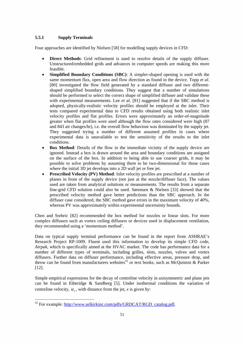
51

5.5.1 Supply Terminals Four approaches are identified by Nielsen [58] for modelling supply devices in CFD:

• Direct Methods: Grid refinement is used to resolve details of the supply diffuser. Unstructured/embedded grids and advances in computer speeds are making this more feasible.

• Simplified Boundary Conditions (SBC): A simpler-shaped opening is used with the same momentum flux, open area and flow direction as found in the device. Topp et al. [80] investigated the flow field generated by a standard diffuser and two different-shaped simplified boundary conditions. They suggest that a number of simulations should be performed to select the correct shape of simplified diffuser and validate these with experimental measurements. Lee et al. [81] suggested that if the SBC method is adopted, physically-realistic velocity profiles should be employed at the inlet. Their tests compared experimental data to CFD results obtained using both realistic inlet velocity profiles and flat profiles. Errors were approximately an order-of-magnitude greater when flat profiles were used although the flow rates considered were high (87 and 843 air changes/hr), i.e. the overall flow behaviour was dominated by the supply jet. They suggested trying a number of different assumed profiles in cases where experimental data is unavailable to test the sensitivity of the results to the inlet conditions.

• Box Method: Details of the flow in the immediate vicinity of the supply device are ignored. Instead a box is drawn around the area and boundary conditions are assigned on the surface of the box. In addition to being able to use coarser grids, it may be possible to solve problems by assuming them to be two-dimensional for those cases where the initial 3D jet develops into a 2D wall jet or free jet.

• Prescribed Velocity (PV) Method: Inlet velocity profiles are prescribed at a number of planes in front of the supply device (not just at the nozzle/diffuser face). The values used are taken from analytical solutions or measurements. The results from a separate fine-grid CFD solution could also be used. Sørensen & Nielsen [33] showed that the prescribed velocity method gave better predictions than the SBC approach. In the diffuser case considered, the SBC method gave errors in the maximum velocity of 40%, whereas PV was approximately within experimental uncertainty bounds.

Chen and Srebric [82] recommended the box method for nozzles or linear slots. For more complex diffusers such as vortex ceiling diffusers or devices used in displacement ventilation, they recommended using a ‘momentum method’. Data on typical supply terminal performance can be found in the report from ASHRAE’s Research Project RP-1009. Fluent used this information to develop its simple CFD code, Airpak, which is specifically aimed at the HVAC market. The code has performance data for a number of different types of terminals, including grilles, slots, nozzles, valves and vortex diffusers. Further data on diffuser performance, including effective areas, pressure drop, and throw can be found from manufacturers websites32 or text books, such as McQuiston & Parker [12]. Simple empirical expressions for the decay of centreline velocity in axisymmetric and plane jets can be found in Etheridge & Sandberg [5]. Under isothermal conditions the variation of centreline velocity, cu , with distance from the jet, x is given by:

32 For example: http://www.selkirkinc.com/pdfs/GRDCAT/RGD_catalog.pdf.

52

• Axisymmetric: x

ACu

xuc 1)(

0

=

• Two-dimensional jet: x

ACu

xuc 1)(

0

=

where 0u is the initial velocity, A is the free area of the terminal and C is a coefficient which depends on the supply Archimedes number and geometry, and is usually determined experimentally. Devices which spread out the air radially have lower C values (i.e. the centreline velocity decreases more rapidly). There are no standards for determining C for non-isothermal flows so commonly the isothermal values are used for non-isothermal flows [5]. Further details of these simplified empirical models are available in ASHRAE Fundamentals Chapter 32: Space Air Diffusion. It is not clear how much the design of the extract terminal affects the flow in the room. McQuiston & Parker [12] suggest that the construction of an extract grille has very little to do with the overall performance except to introduce a pressure drop and some noise if incorrectly sized. Etheridge & Sandberg [5] describe a simple model that predicts the velocity distribution near an exhaust. The velocity is shown to decrease to one-tenth of the face velocity within one diameter of the exhaust. They note, however, that stratification within the room can cause the location of the extract to have a significant affect on the overall flow pattern within the room.

5.5.2 Occupants A variety of different models have been used to simulate occupants in indoor air simulations. Peng and Davidson [8] simulated a person as a simplified standing manikin shape, 1.7 m high with discernable head, arms, torso and legs. Nielsen [58] used two different models, an S-shaped cuboid called CSP1 (Computer Simulated Person 1) and a physically-realistic human shape CSP2. Results for the flow close to the bodies were significantly different due to the flat sides and sharp edges of CSP1 and its lack of separate limbs. Concentrations at head level were different by a factor of two or more. Some distance away from the manikins, however, the flow was fairly similar. Nielsen suggested that the detailed model should be used for local air quality problems such as passive smoking and cross-infection, whereas the simplified models can be used for studies of global velocity, concentration and temperature variations in a room. Etheridge & Sandberg [5] noted that for a person standing in a room with displacement ventilation, the boundary layer around the body near the floor is laminar. As the air is heated up and drawn up the body due to buoyancy, the boundary layer undergoes transition to turbulent flow. They report that the boundary layer thickness under these conditions is typically around 18 cm thick at head height, where the maximum velocity is about 0.5 m/s about 2 cm from the skin surface. These figures can be used to provide some guidance on grid resolution.

5.5.3 Surface Roughness & Porosity Generating computational grids around room obstacles such as furniture is often impractical. An alternative approach is to use a porosity model or source terms in the momentum equations to account for the blocking effect of obstacles. Small projections from walls can also be modelled as an effective wall roughness.

53

Data on these treatments are scarce. Much of the literature on porosity is aimed at flow through granular media rather than large-scale highly anisotropic structures such as office furniture. Likewise, there is little data on how to calibrate wall-roughness modifications of wall functions for application to indoor air flows. Nielsen [58] discussed one example where furniture and other obstacles are modelled as an additional pressure drop in the momentum equations. Results were compared for scenarios with and without furniture. Details of this approach are provided in [83]. The pressure drop, dP/dx, was calibrated to provide the best fit between CFD results and experiments. The new source term in the momentum equations was given by:

2

2uf

xP ρ=

∂∂

where the optimum value for the loss coefficient, f, was found to be 0.5 m-1. This value was used in all three coordinate directions. The sensitivity of CFD results to the value of the loss coefficient was not explored. Nielsen et al. [83] also provided an empirical expression relating the reduction in maximum velocity in the occupied zone to the total length of furniture volume. For data on the deposition of particulate contaminants on walls with different surface roughness, see Lai et al. [84].

5.5.4 Overall Grid Resolution There are no generally applicable rules for determining a priori the optimum location of grid cells in CFD simulations. Adaptive meshing techniques, where the grid is refined automatically as the calculation progresses in order to minimize an error condition, are not widely used. Instead, it is usually recommended that a grid-refinement study is performed, running the same simulation with finer grids up to the point where the results show no significant differences from increasing further the number of cells. This practice is not always possible in large transient calculations where the high computing cost precludes multiple runs. Estimating the inaccuracy in results due to poor grid resolution is not generally possible. One example of a situation where grid-refinement led to significant changes in results is Ward & Wang’s [85] simulations of buoyancy and wind-driven flow inside a parish church building. They used two levels of grid resolution and found that the overall air flow pattern changed considerably, resulting in complete flow reversal in one region. They attributed this difference to the ability of the finer grid to resolve more accurately the convective heat transfer at the radiator surface.

5.6 INFILTRATION The majority of CFD models of indoor air flows neglect infiltration. Two notable exceptions are Ward and Wang’s [85] model of a parish church which explicitly accounted for gaps around the windows and Foster et al.’s [86] study of infiltration through cold-store entrances. In general, this approach is impractical due to constraints on the mesh quality around such fine-scale structures and the overall number of grid nodes.

54

If infiltration is included in the CFD model, it may be inaccurate to assume that air leaking into the space is at the outside ambient temperature. A CFD study by Abadie et al. [87] suggested that the building fabric acts as a heat exchanger, increasing the temperature of outside cool air as it infiltrates through cracks into the interior space. Beausoleil-Morrison et al. [88] describe a model which accounted for infiltration by coupling CFD to a simple zonal approach.

55

6 CONCLUSIONS

This report has described the main factors affecting contaminant dispersion in rooms. Information has been provided on how to quantify the relative importance of different factors and how to characterize the distribution of contaminants in rooms. Guidance has also been given on the inclusion of these factors in CFD models. A number of topics require further investigation. Results from both the literature and preliminary in-house tests have shown that thermal radiation can have a significant effect on air movement and contaminant transport. Two studies have also shown that the distribution of water vapour in the room atmosphere, i.e. humidity, significantly affects the air flow pattern. These two factors should be investigated in more depth. The report has not considered in detail how particulate contaminants are modelled in CFD. There are a number of alternative approaches available: discrete particle-tracking, Monte-Carlo methods, Eulerian moments etc. The best approach for a given situation depends on the properties of the contaminant, its concentration and the information required. It is advised to investigate further aerosols modelling appropriate to cover the scenarios of interest to HSE. It is also recommended that expertise in modelling contaminant dispersion be kept up-to-date through periodical reviews of the literature. New developments likely to address HSE’s needs should be assessed on a regular basis using case studies close to HSE’s scenarios of interest.

56

7 BIBLIOGRAPHY

1. Lea, C.J., Guidance for NSD on the assessment of CFD simulations in safety cases, in HSL Report FS/97/8. 1997.

2. Gobeau, N.C.H., H.S. Ledin, and C.J. Lea, Guidance for HSE Inspectors: Smoke movement in complex enclosed spaces - Assessment of computational fluid dynamics, in HSE Research Report. 2003.

3. Gobeau, N., C.J. Lea, A. Kelsey, and C.J. Saunders, Investigation of the factors influencing pesticide distribution in naturally ventilated buildings. 2005, Health & Safety Laboratory Report CM/05/12.

4. Deevy, M.T. and N.G. Gobeau, Developing expertise for modelling dispersion of hazardous substances with simple models. 2005, Health & Safety Laboratory Report CM/05/09.

5. Etheridge, D. and M. Sandberg, Building Ventilation: Theory and Measurement. 1996: John Wiley & Sons Ltd.

6. Linden, P.F., The fluid mechanics of natural ventilation. Annu. Rev. Fluid Mech., 1999. 31: p. 201-238.

7. Goodfellow, H. and E. Tähti, Industrial Ventilation: Design Guidebook. 2001: Academic Press.

8. Peng, S.-H. and L. Davidson. Performance evaluation of a displacement ventilation system for improving indoor air quality: a numerical study. in 8th International Conference on Indoor Air Quality and Climate. 1999. Edinburgh, Scotland.

9. Heiselberg, P. and M. Sandberg. Convection from a slender cylinder in a ventilated room. in Roomvent '90. 1990. Oslo, Norway.

10. CIBSE, Ventilation and Air Conditioning. Guide B2. 2001.

11. ASHRAE, Handbook: HVAC Systems & Equipment (2000), Fundamentals (2001), Refrigeration (2002) and HVAC Applications (2003).

12. McQuiston, F.C. and J.D. Parker, Heating, Ventilation and Air Conditioning: Analysis and Design. Fourth ed. 1994: John Wiley & Sons, Inc.

13. Carrer, P., Y. Bruinen de Bruin, M. Franchi, and E. Valovirta. The EFA Project: indoor air quality in European schools. in Indoor Air. 2002. Monterey, California, U.S.

14. Meyer, B., Indoor Air Quality. 1983: Addison-Wesley, Reading, MA, USA.

15. Norbäck, D., K. Ancker, and G. Johanson, Field evaluation of CO2 detector tubes for measuring outdoor air supply rate in the indoor environment. Indoor Air, 1992. 2: p. 58-64.

16. Johnson, R.W., The Handbook of Fluid Dynamics. 1998: CRC Press LLC.

57

17. Cebeci, T. and P. Bradshaw, Physical and computational aspects of convective heat transfer. 1984: Springer-Verlag New York Inc.

18. Zhang, Y. and F. Haghighat, The impact of surface air movement on material emissions. Building and Environment, 1997. 32(6): p. 551-556.

19. Stymme, H., M. Sandberg, and M. Mattsson. Dispersion pattern of contaminants in a displacement - implications for demand control. in 12th AIVC Conference. 1991. Ottawa, Canada.

20. Tennekes, H. and J.L. Lumley, A First Course in Turbulence. 1974: MIT Press.

21. Howell, S.A. and I. Potts. On the natural displacement ventilation flow through a full scale enclosure, driven by a source of buoyancy at floor level. in Seventh International IBPSA Conference. 2001. Rio de Janeiro, Brazil.

22. Kaye, N.B. and G.R. Hunt, Time-dependent flows in an emptying filling box. J. Fluid Mech., 2004. 520: p. 135-156.

23. Mattsson, M. and M. Sandberg. Displacement ventilation - influence of physical activity. in RoomVent '94. 1994. Krakow, Poland.

24. Kiel, D.E. and D.J. Wilson, Combining door swing pumping with density driven flow. ASHRAE Transactions, 1989. 95(2): p. 590-599.

25. Nimmermark, S. and G. Gustafsson, Influence of temperature, humidity and ventilation rate on the release of odour and ammonia in a floor housing system for laying hens. CIGR Journal of Scientific Research and Development, BC 04 008, 2005. 7: p. 1-14.

26. Di Tommaso, R.M., E. Nino, and G.V. Fracastoro, Influence of the boundary thermal conditions on the air change efficiency indexes. Indoor Air, 1999. 9: p. 63-69.

27. Peng, S.-H., S. Holmberg, and L. Davidson, On the assessment of ventilation performance with the aid of numerical simulations. Building & Environment, 1997. 32(6): p. 497-508.

28. Peng, S.-H. and L. Davidson, Towards the determination of regional purging flow rate. Building & Environment, 1997. 32(6): p. 513-525.

29. Sandberg, M. and M. Sjoberg, The use of moments for assessing air quality in ventilated rooms. Building & Environment, 1983. 18: p. 181-197.

30. Zhang, Y., X. Wang, G.L. Riskowski, and L.L. Christianson, Quantifying ventilation effectiveness for air quality control. Transactions of the American Society of Agricultural and Biological Engineers (ASABE), 2001. 44(2): p. 385-390.

31. Durbin, P.A. and B.A. Pettersson Reif, Statistical theory and modeling for turbulent flows. 2001: John Wiley & Sons.

32. Gobeau, N., Review of simple deterministic models predicting the indoor concentration of a contaminant, in HSL report. 2004.

33. Sørensen, D.N. and P.V. Nielsen, Quality control of computational fluid dynamics in indoor environments. Indoor Air, 2003. 13: p. 2-17.

58

34. Pope, S.B., Turbulent Flows. 2000: Cambridge University Press.

35. Launder, B.E. and N.D. Sandham, Closure Strategies for Turbulent and Transitional Flows. 2002: Cambridge University Press.

36. Sagaut, P., Large-Eddy Simulation for Incompressible Flows. An Introduction. 2001: Heidelberg: Springer.

37. Baggett, J.S., J. Jiménez, and A.G. Kravchenko, Resolution requirements in large-eddy simulations of shear flows, in Annual Research Briefs. 1997, Stanford Centre for Turbulence Research.

38. Cowan, J.R. and P. Gallagher, Review of the applicability of the large eddy simulation technique to safety studies, in WSA Report AM5226/R1. 1999, WS Atkins Science & Technology.

39. Kempf, A., R.P. Lindstedt, and J. Janicka, Large-eddy simulation of a bluff-body stabilized nonpremixed flame. Combustion and Flame, 2006. 144: p. 170-189.

40. Addad, Y., S. Benhamadouche, and D. Laurence. The Negatively Buoyant Wall-Jet. Part 1: LES Database. in Turbulence, Heat and Mass Transfer 4. 2003: Begell House, Inc.

41. Mittal, R. and P. Moin, Suitability of upwind-biased finite difference schemes for LES of turbulent flow. AIAA Journal, 1997. 35(8): p. 1415-1417.

42. Menter, F.R., M. Kuntz, and R. Bender. A scale-adaptive simulation model for turbulent flow predictions. in 41st Aerospace Science Meeting & Exhibit. 2003. Reno, Nevada, USA.

43. Craft, T.J., S.E. Gant, H. Iacovides, and B.E. Launder, A new wall function strategy for complex turbulent flows. Numerical Heat Transfer, Part B: Fundamentals, 2004. 45(4): p. 301-318.

44. Mayle, R.E., The role of laminar-turbulent transition in gas turbine engines. J. Turbomachinery, 1991. 113: p. 509-537.

45. Savill, A.M., Some recent progress in the turbulence modelling of by-pass transition, in Near-wall turbulent flows, R.M.C. So, C.G. Speziale, and B.E. Launder, Editors. 1993, Elsevier Science Publishers B. V. p. 829-848.

46. Savill, A.M., By-pass transition using conventional closures, in Closure strategies for turbulent and transitional flows, B.E. Launder and N.D. Sandham, Editors. 2002, Cambridge University Press. p. 464-492.

47. Savill, A.M., New strategies in modelling by-pass transition, in Closure strategies for turbulent and transitional flows, B.E. Launder and N.D. Sandham, Editors. 2002, Cambridge University Press. p. 493-521.

48. Jones, W.P. and B.E. Launder, The prediction of laminarization with a two-equation model of turbulence. Int. J. Heat Mass Transfer, 1972. 15: p. 301-314.

49. Schlatter, P., S. Stolz, and L. Kleiser, LES of transitional flows using the approximate deconvolution model. Int. J. Heat Fluid Flow, 2004. 25(3): p. 549-558.

59

50. Moreau, S., F. Mendonca, O. Qazi, R. Prosser, and D. Laurence. Influence of turbulence modeling on airfoil unsteady simulations of broadband noise sources. in 11th AIAA/CEAS Aeroacoustics Conference Meeting and Exhibit. 2005. Monterey, California.

51. Tian, Z.F., J.Y. Tu, and G.H. Yeoh. Large eddy simulation indoor airflow and contaminant concentration. in CTAC2004: the 12th Biennial Computational Techniques & Applications Conference. 2004. University of Melbourne, Victoria, Australia.

52. Luo, X.Y., J.S. Hinton, T.T. Liew, and K.K. Tan, LES modelling of flow in a simple airway model. Medical Engineering & Physics, 2004. 26: p. 403-413.

53. Yang, Z. and P.R. Voke, Large-eddy simulation of transition under turbulence, in Report ME-FD/93.13. 1993, Dept. of Mechanical Engineering, University of Surrey, Guildford, UK.

54. Durbin, P.A., On the k-ε stagnation point anomaly. Int. J. Heat Fluid Flow, 1995. 17: p. 89-90.

55. Craft, T.J., L.J.W. Graham, and B.E. Launder, Impinging jet studies for turbulence model assessment - II. An examination of the performance of four turbulence models. Int. J. Heat Mass Transfer, 1993. 36(10): p. 2685-2697.

56. Cziesla, T., G. Biswas, H. Chattopadhyay, and N.K. Mitra, Large-eddy simulation of flow and heat transfer in an impinging slot jet. Int. J. Heat Fluid Flow, 2001. 22(5): p. 500-508.

57. Gao, S. and P.R. Voke, Large-eddy simulation of turbulent heat transport in enclosed impinging jets. Int. J. Heat Fluid Flow, 1995. 16(5): p. 349-356.

58. Nielsen, P.V., Computational fluid dynamics and room air movement. Indoor Air, 2004. 14(7): p. 134-143.

59. Demeuren, A.O. and W. Rodi, Calculation of turbulence-driven secondary motion in non-circular ducts. J. Fluid Mech., 1984. 140: p. 189-222.

60. Speziale, C.G., On nonlinear k-l and k-ε models of turbulence. J. Fluid Mech., 1987. 178: p. 459-475.

61. Lübcke, H.M., T. Rung, and F. Thiele, Prediction of the spreading mechanism of 3D turbulent wall jets with explicit Reynolds-stress closures. Int. J. Heat Fluid Flow, 2003. 24: p. 434-443.

62. Madabhushi, R.K. and S.P. Vanka, Large eddy simulation of turbulence-driven secondary flow in a square duct. Phys. Fluids, 1991. 3(11): p. 2734-2745.

63. George, D.K., M.R. Flynn, and R. Goodman, The impact of boundary layer separation on local exhaust design and worker exposure. Appl. Occup. Environ. Hyg., 1990. 5(8): p. 501-509.

64. Dunnett, S.J., A numerical investigation into the flow field around a worker positioned by an exhaust opening. Ann. Occup. Hyg., 1994. 38(5): p. 663-686.

60

65. Rodi, W., Large-eddy simulation of the flow past bluff bodies, in Closure strategies for turbulent and transitional flows, B.E. Launder and N.D. Sandham, Editors. 2002, Cambridge University Press. p. 361-391.

66. Murakami, S., A. Mochida, R. Ooka, S. Kato, and S. Iizuka, Numerical prediction of flow around a building with various turbulence models. ASHRAE Transactions, AT-96-10-1, 1996.

67. Pope, S.B., An explanation of the turbulent round-jet/plane-jet anomaly. AIAA Journal, 1978. 16(3): p. 279-281.

68. Younis, B.A., T.B. Gatski, and C.G. Speziale, Assessment of the SSG pressure-strain model in free turbulent jets with and without swirl. J. Fluids Eng., 1996. 118(4): p. 800-809.

69. Fatica, M., P. Orlandi, and R. Verzicco, Direct and large eddy simulation of round jets, in Direct and Large-Eddy Simulation, P.R. Voke, Editor. 1994, Kluwer Academic Publishers. p. 49-60.

70. Saidi, M.H. and M. Hendijanifard. 3D Contaminant removal improvement from a typical clean room. in Fourth International Conference on Computational Heat & Mass Transfer (ICCHMT). 2005. ENS-Cachan, Paris, France.

71. Flesch, T.K., J.H. Prueger, and J.L. Hatfield, Turbulent Schmidt number from a tracer experiment. Agricultural and Forest Meteorology, 2002. 111: p. 299-307.

72. Ivings, M.J., M. Azhar, C. Carey, C.J. Lea, S. Ledin, Y. Sinai, C. Skinner, and P. Stephenson, Outstanding Safety Questions Concerning the Use of Gas Turbines for Power Generation: Final Report on the CFD Modelling Programme of Work, in Project Report. 2003, HSL.

73. Yimer, I., I. Campbell, and L.-Y. Jiang, Estimation of the turbulent Schmidt number from experimental profiles of axial velocity and concentration for high-Reynolds-number jet flows. Canadian Aeronautics and Space Journal, 2002. 48(3): p. 195-200.

74. Bird, R.B., W.E. Stewart, and E.N. Lightfoot, Transport Phenomena. Wiley International Editions. 1960: John Wiley & Sons, Inc.

75. Worthy, J., V. Sanderson, and P.A. Rubini, A comparison of modified k-ε models for buoyant plumes. Numerical Heat Transfer, Part B: Fundamentals, 2001. 39(2): p. 151-166.

76. Lu, W., A.T. Howarth, and A.P. Jeary, Prediction of airflow and temperature field in a room with convective heat source. Building and Environment, 1997. 32(6): p. 541-550.

77. Rodi, W., Turbulence models and their applications in hydraulics - a state of the art review. 1980, Institut für Hyromechanik: Universität Karlsruhe, Germany.

78. Misirlioglu, A. and U. Gulcat. Modified displacement ventilation of rooms with chilled ceilings and ceiling mounted devices. in 4th International Conference on Computational Heat & Mass Transfer. 2005. ENS-Cachan, Paris, France: Lavoisier.

61

79. Teodosiu, C., R. Hohota, G. Rusaouën, and M. Woloszyn, Numerical prediction of indoor air humidity and its effect on indoor environment. Building and Environment, 2003. 38: p. 655-664.

80. Topp, C., R.L. Jensen, D.N. Pedersen, and P.V. Nielsen. Validation of boundary conditions for CFD simulations on ventilated rooms. in 4th International Conference on Indoor Air Quality, Ventilation and Energy Conservation. 2001. Hunan University.

81. Lee, E., C.E. Feigley, and J. Khan, An investigation of air inlet velocity in simulating dispersion of indoor contaminants via computation fluid dynamics. Ann. Occup. Hyg., 2002. 46(8): p. 701-712.

82. Chen, Q. and J. Srebric, Simplified Diffuser Boundary Conditions for Numerical Room Airflow Models, in ASHRAE RD-1009. 2001.

83. Nielsen, J.R., P.V. Nielsen, and K. Svidt. The influence of furniture on air velocity ain a room - an isothermal case. in Roomvent '98: Sixth International Conference on Air Distribution in Rooms. 1998. Stockholm, Sweden.

84. Lai, A.C.K., M.A. Byrne, and A.J.H. Goddard, Experimental studies of the effect of rough surfaces and air speed on aerosol deposition in a test chamber. Aerosol Sci. & Tech., 2002. 36: p. 973-982.

85. Ward, I.C. and F. Wang. Air movement studies in a large parish church building. in The Role of Ventilation, 15th AIVC Conference. 1994. Buxton, UK.

86. Foster, A.M., M.J. Swain, R. Barrett, and S.J. James, Experimental verification of analytical and CFD predictions of infiltration through cold store entrances. International Journal of Refrigeration, 2003. 26: p. 918-925.

87. Abadie, M.O., E.U. Finlayson, and A.J. Gadgil, Infiltration heat recovery in building walls: computational fluid dynamics investigations results, in LBNL-51324. 2002, Energy Performace of Buildings Group, Lawrence Berkeley National Lab, U.S. (http://epb.lbl.gov).

88. Beausoleil-Morrison, I., J.A. Clarke, J. Denev, I.A. MacDonald, A. Melikov, and P. Stankov. Further developments in the conflation of CFD and building simulation. in Seventh International IBPSA Conference. 2001. Rio de Janeiro, Brazil.