A VARIATIONAL FORMULATION FOR

FRAME-BASED INVERSE PROBLEMS∗

Caroline Chaux,1 Patrick L. Combettes,2 Jean-Christophe Pesquet,1

and Valerie R. Wajs2

1Institut Gaspard Monge and UMR CNRS 8049

Universite de Marne la Vallee

77454 Marne la Vallee Cedex 2, France

2Laboratoire Jacques-Louis Lions – UMR CNRS 7598

Faculte de Mathematiques

Universite Pierre et Marie Curie – Paris 6

75005 Paris, France

May 5, 2007

Abstract

A convex variational framework is proposed for solving inverse problems in Hilbert spaceswith a priori information on the representation of the target solution in a frame. The objectivefunction to be minimized consists of a separable term penalizing each frame coefficient individ-ually and of a smooth term modeling the data formation model as well as other constraints.Sparsity-constrained and Bayesian formulations are examined as special cases. A splitting algo-rithm is presented to solve this problem and its convergence is established in infinite-dimensionalspaces under mild conditions on the penalization functions, which need not be differentiable.Numerical simulations demonstrate applications to frame-based image restoration.

1 Introduction

In inverse problems, certain physical properties of the target solution x are most suitably expressedin terms of the coefficients (ξk)k∈K⊂N of its representation x =

∑

k∈Kξkek with respect to a

family of vectors (ek)k∈K in a Hilbert space (H, ‖ · ‖). Traditionally, such linear representationshave been mostly centered on orthonormal bases as, for instance, in Fourier, wavelet, or bandletdecompositions [8, 25, 26]. Recently, attention has shifted towards more general, overcompleterepresentations known as frames; see [6, 7, 16, 20, 33] for specific examples. Recall that a family

∗Contact author: P. L. Combettes, plc@math.jussieu.fr, phone: +33 1 4427 6319, fax: +33 1 4427 7200.

1

of vectors (ek)k∈K in H constitutes a frame if there exist two constants µ and ν in ]0,+∞[ suchthat

(∀x ∈ H) µ‖x‖2 ≤∑

k∈K

|〈x | ek〉|2 ≤ ν‖x‖2. (1.1)

The associated frame operator is the injective bounded linear operator

F : H → ℓ2(K) : x 7→ (〈x | ek〉)k∈K, (1.2)

the adjoint of which is the surjective bounded linear operator

F ∗ : ℓ2(K) → H : (ξk)k∈K 7→∑

k∈K

ξkek. (1.3)

When µ = ν in (1.1), (ek)k∈K is said to be a tight frame. A simple example of a tight frame isthe union of m orthonormal bases, in which case µ = ν = m. For instance, in H = L2(R2), a realdual-tree wavelet decomposition is the union of two orthonormal wavelet bases [7, 30]. Curvelets[6] constitute another example of a tight frame of L2(R2). Historically, Gabor frames [16, 33] haveplayed an important role in many inverse problems. Another common example of a frame is aRiesz basis, which corresponds to the case when (ek)k∈K is linearly independent or, equivalently,when F is bijective. In such instances, there exists a unique Riesz basis (ek)k∈K such that (ek)k∈K

and (ek)k∈K are biorthogonal. Furthermore, for every x ∈ H and (ξk)k∈K ∈ ℓ2(K),

x = F ∗(ξk)k∈K ⇔ (∀k ∈ K) ξk = 〈x | ek〉. (1.4)

When F−1 = F ∗, (ek)k∈K is an orthonormal basis and (ek)k∈K = (ek)k∈K. Examples of Rieszbases of L2(R2) include biorthogonal bases of compactly supported dyadic wavelets having certainsymmetry properties [9]. Further constructions as well as a detailed account of frame theory inHilbert spaces can be found in [23].

The goal of the present paper is to propose a flexible convex variational framework for solvinginverse problems in which a priori information (e.g., sparsity, distribution, statistical properties) isavailable about the representation of the target solution in a frame. Our analysis and our numer-ical algorithm will rely heavily on proximity operators. Section 2 is devoted to these operators.Our main variational formulation is presented and analyzed in Section 3. It consists (see Prob-lem 3.1) of minimizing the sum of a separable, possibly nondifferentiable function penalizing eachcoefficient of the frame decomposition individually, and of a smooth function which combines otherinformation on the problem and the data formation model. Connections with sparsity-constrainedand Bayesian formulations are also established. In connection with the latter, we derive in Sec-tion 4 closed-form expressions for the proximity operators associated with a variety of univariatelog-concave distributions. A proximal algorithm for solving Problem 3.1 is presented in Section 5and its convergence is established in infinite-dimensional spaces under mild assumptions on thepenalization functions. An attractive feature of this algorithm is that it is fully split in that,at each iteration, all the functions appearing in the problem are activated individually. Finally,applications to image recovery are demonstrated in Section 6.

2

2 Basic tool: proximity operator

2.1 Notation

Throughout, X is a separable real Hilbert space with scalar product 〈· | ·〉, norm ‖ ·‖, and distanced. Γ0(X ) is the class of lower semicontinuous convex functions from X to ]−∞,+∞] which are notidentically equal to +∞. The indicator function of a subset S of X is

ιS : x 7→

0, if x ∈ S;

+∞, if x /∈ S,(2.1)

its support function is σS : X → [−∞,+∞] : u 7→ supx∈S 〈x | u〉, and its distance function isdS : X → [0,+∞] : x 7→ inf ‖S − x‖. If S is nonempty, closed, and convex then, for every x ∈ X ,there exists a unique point PSx in S, called the projection of x onto S, such that ‖x−PSx‖ = dS(x)(further background on convex analysis will be found in [36]).

2.2 Background

Let ϕ ∈ Γ0(X ). The subdifferential of ϕ at x ∈ X is the set

∂ϕ(x) =

u ∈ X∣

∣ (∀y ∈ X ) 〈y − x | u〉 + ϕ(x) ≤ ϕ(y)

. (2.2)

If ϕ is Gateaux differentiable at x with gradient ∇ϕ(x), then ∂ϕ(x) = ∇ϕ(x). The conjugate ofϕ is the function ϕ∗ ∈ Γ0(X ) defined by

(∀u ∈ X ) ϕ∗(u) = supx∈X

〈x | u〉 − ϕ(x). (2.3)

The continuous convex function

γϕ : X → R : x 7→ infy∈X

ϕ(y) +1

2γ‖x − y‖2 (2.4)

is the Moreau envelope of index γ ∈ ]0,+∞[ of ϕ.

Definition 2.1 [28] Let ϕ ∈ Γ0(X ). Then, for every x ∈ X , the function y 7→ ϕ(y) + ‖x − y‖2/2achieves its infimum at a unique point denoted by proxϕ x. The operator proxϕ : X → X thusdefined is the proximity operator of ϕ. Moreover,

(∀x ∈ X )(∀p ∈ X ) p = proxϕ x ⇔ x − p ∈ ∂ϕ(p) (2.5)

⇔ (∀y ∈ X ) 〈y − p | x − p〉 + ϕ(p) ≤ ϕ(y). (2.6)

Example 2.2 Let γ ∈ ]0,+∞[, let S be a nonempty convex subset of X , and set ϕ = ιS . Then itfollows at once from (2.1), (2.4), and Definition 2.1 that γϕ = d2

S/(2γ) and proxγϕ = PS .

Here are basic properties of the proximity operator.

3

Lemma 2.3 [15, Section 2] Let ϕ ∈ Γ0(X ). Then the following hold.

(i) (∀x ∈ X ) x ∈ Argminϕ ⇔ 0 ∈ ∂ϕ(x) ⇔ proxϕ x = x.

(ii) (∀x ∈ X )(∀y ∈ X ) ‖proxϕ x − proxϕ y‖ ≤ ‖x − y‖.

(iii) (∀x ∈ X )(∀γ ∈ ]0,+∞[) x = proxγϕ x + γ proxϕ∗/γ(x/γ).

In Lemma 2.3, (i) states that the minimizers of ϕ are characterized as the zeros of the subdif-ferential of ϕ (Fermat’s rule) or, equivalently, as the fixed points of proxϕ; (ii) states that proxϕ isnonexpansive, which turns out to be an essential property in the convergence of iterative methods[13]; finally, (iii) is Moreau’s decomposition principle [27], which provides a powerful nonlineardecomposition rule parametrized by ϕ and extends in particular the standard orthogonal decom-position rule [15, Remark 2.11].

Lemma 2.4 Let ϕ ∈ Γ0(X ), let γ ∈ ]0,+∞[, and set ψ = γϕ. Then the following hold.

(i) ψ is Frechet-differentiable on X .

(ii) ∇ψ = (Id − proxγϕ)/γ = proxϕ∗/γ(·/γ).

(iii) ∇ψ is (1/γ)-Lipschitz continuous.

Proof. (i) and (ii): A routine extension of [28, Proposition 7.d], where γ = 1. (iii): Since ϕ∗/γ ∈Γ0(X ) and (ii) asserts that ∇ψ = proxϕ∗/γ(·/γ), this is a direct consequence of Lemma 2.3(ii).

Next, we record some proximal calculus rules that will allow us to derive new proximity operatorsfrom existing ones.

Lemma 2.5 [15, Lemma 2.6] Let ϕ ∈ Γ0(X ) and let x ∈ X . Then the following hold.

(i) Let ψ = ϕ+ α‖ · ‖2/2 + 〈· | u〉 + β, where u ∈ X , α ∈ [0,+∞[, and β ∈ R. Then proxψ x =proxϕ/(α+1)

(

(x − u)/(α + 1))

.

(ii) Let ψ = ϕ(· − z), where z ∈ X . Then proxψ x = z + proxϕ(x − z).

(iii) Let ψ = ϕ(·/ρ), where ρ ∈ R r 0. Then proxψ x = ρproxϕ/ρ2(x/ρ).

(iv) Let ψ : y 7→ ϕ(−y). Then proxψ x = − proxϕ(−x).

We conclude this section with some properties of proximity operators on the real line.

Lemma 2.6 Let φ ∈ Γ0(R). Then the following hold.

(i) [14, Proposition 2.4] proxφ : R → R is increasing.

4

(ii) [14, Corollary 2.5] Suppose that φ admits 0 as a minimizer. Then

(∀ξ ∈ R)

0 ≤ proxφ ξ ≤ ξ, if ξ > 0;

proxφ ξ = 0, if ξ = 0;

ξ ≤ proxφ ξ ≤ 0, if ξ < 0.

(2.7)

This is true in particular when φ is even.

(iii) [14, Proposition 3.6] Suppose that φ = ψ + σΩ, where ψ ∈ Γ0(R) is differentiable at 0 with

ψ′(0) = 0, and where Ω ⊂ R is a nonempty closed interval. Then proxφ = proxψ softΩ ,

where

softΩ = proxσΩ: R → R : ξ 7→

ξ − ω, if ξ < ω;

0, if ξ ∈ Ω;

ξ − ω, if ξ > ω,

with

ω = inf Ω,

ω = supΩ,(2.8)

is the soft thresholder on Ω. In particular, if Ω = [−ω, ω] for some ω ∈ ]0,+∞[, we obtain

soft[−ω,ω] = proxω|·| : R → R : ξ 7→ sign(ξ)max|ξ| − ω, 0. (2.9)

The soft-thresholding operation described in Lemma 2.6(iii) is illustrated in Fig. 1.

2.3 Forward-backward splitting

In this section, we consider the following abstract variational framework, that will cover our mainproblem (Problem 3.1).

Problem 2.7 Let f1 and f2 be functions in Γ0(X ) such that f2 is differentiable on X with aβ-Lipschitz continuous gradient for some β ∈ ]0,+∞[. The objective is to

minimizex∈X

f1(x) + f2(x). (2.10)

A key consequence of Fermat’s rule (Lemma 2.3(i)) and (2.5) is the following characterization ofthe solutions to Problem 2.7 which, in itself, attests the central role played by proximity operators.

Proposition 2.8 [15, Proposition 3.1(iii)] Let x ∈ X and let γ ∈ ]0,+∞[. Then x is a solution to

Problem 2.7 if and only if x = proxγf1(

x − γ∇f2(x))

.

Let γ ∈ ]0,+∞[ and set T = proxγf1 (Id −γ∇f2). Proposition 2.8 asserts that a point x ∈ Xsolves Problem 2.7 if and only if x = T x. This fixed point characterization suggests solvingProblem 2.7 via the successive approximation method xn+1 = T xn, for suitable values of the“step size” parameter γ. The next result describes an algorithm in this vein, which is basedon the forward-backward splitting method for monotone operators [13]. It allows for inexactevaluations of the operators proxf1 and ∇f2 via the incorporation of the error sequences (an)n∈N

and (bn)n∈N, respectively, as well as for iteration-dependent relaxation parameters (λn)n∈N andstep sizes (γn)n∈N.

5

Theorem 2.9 [15, Theorem 3.4(i)] Suppose that Argmin(f1 +f2) 6= ∅. Let (γn)n∈N be a sequence

in ]0,+∞[ such that 0 < infn∈N γn ≤ supn∈N γn < 2/β, let (λn)n∈N be a sequence in ]0, 1] such that

infn∈N λn > 0, and let (an)n∈N and (bn)n∈N be sequences in X such that∑

n∈N‖an‖ < +∞ and

∑

n∈N‖bn‖ < +∞. Fix x0 ∈ X and, for every n ∈ N, set

xn+1 = xn + λn

(

proxγnf1

(

xn − γn(∇f2(xn) + bn))

+ an − xn

)

. (2.11)

Then (xn)n∈N converges weakly to a solution to Problem 2.7.

2.4 Decomposition formula

The following decomposition property, which extends [15, Example 2.19], will be instrumental inour analysis.

Proposition 2.10 Set Υ: X → ]−∞,+∞] : x 7→∑

i∈Iψi(〈x | oi〉), where:

(i) ∅ 6= I ⊂ N;

(ii) (oi)i∈I is an orthonormal basis of X ;

(iii) (ψi)i∈I are functions in Γ0(R);

(iv) Either I is finite, or there exists a subset J of I such that:

(a) I r J is finite;

(b) (∀i ∈ J) ψi ≥ 0;

(c) there exists a sequence (ζi)i∈J in R such that∑

i∈J|ζi|2 < +∞,

∑

i∈J|proxψi

ζi|2 < +∞,

and∑

i∈Jψi(ζi) < +∞.

Then Υ ∈ Γ0(X ) and (∀x ∈ X ) proxΥ x =∑

i∈I

(

proxψi〈x | oi〉

)

oi.

Proof. We treat only the case when I is infinite as the case when I is finite will follow triviallythe arguments presented below. Fix, for every i ∈ I r J, ζi ∈ R such that ψi(ζi) < +∞ and setz =

∑

i∈Iζioi. Then (iv) implies that

∑

i∈Iζ2i < +∞ and, in view of (ii), that z ∈ X . Moreover,

Υ(z) =∑

i∈Jψi(ζi) +

∑

i∈IrJψi(ζi) < +∞.

Let us show that Υ ∈ Γ0(X ). As just seen, Υ(z) < +∞ and, therefore, Υ 6≡ +∞. Next,we observe that, by virtue of (iii), the functions (ψi(〈· | oi〉))i∈I are lower semicontinuous andconvex. As a result,

∑

i∈IrJψi(〈· | oi〉) is lower semicontinuous and convex, as a finite sum of such

functions. Thus, to show that Υ ∈ Γ0(X ), it remains to show that ΥJ =∑

i∈Jψi(〈· | oi〉) is lower

semicontinuous and convex. It follows from (iv)(b) that

ΥJ = supJ′⊂J

J′ finite

∑

i∈J′

ψi(〈· | oi〉). (2.12)

6

However, as above, each finite sum∑

i∈J′ψi(〈· | oi〉) is lower semicontinuous and convex. Therefore,

ΥJ is likewise as the supremum of a family of lower semicontinuous convex functions.

Now fix x ∈ X and set

(∀i ∈ I) ξi = 〈x | oi〉 and πi = proxψiξi. (2.13)

It follows from (iv)(a) and (iv)(c) that∑

i∈I

|proxψiζi|2 =

∑

i∈J

|proxψiζi|2 +

∑

i∈IrJ

|proxψiζi|2 < +∞. (2.14)

Hence, we derive from Lemma 2.3(ii) and (ii) that

1

2

∑

i∈I

|πi|2 ≤∑

i∈I

|πi − proxψiζi|2 +

∑

i∈I

|proxψiζi|2

=∑

i∈I

|proxψiξi − proxψi

ζi|2 +∑

i∈I

|proxψiζi|2

≤∑

i∈I

|ξi − ζi|2 +∑

i∈I

|proxψiζi|2

= ‖x − z‖2 +∑

i∈I

|proxψiζi|2

< +∞. (2.15)

Let us set p =∑

i∈Iπioi. Then it follows from (2.15) and (ii) that p ∈ X . On the other hand, we

derive from (2.13) and (2.6) that

(∀i ∈ I)(∀η ∈ R) (η − πi)(ξi − πi) + ψi(πi) ≤ ψi(η). (2.16)

Hence, by Parseval and (ii),

(∀y ∈ X ) 〈y − p | x − p〉 + Υ(p) =∑

i∈I

〈y − p | oi〉〈x − p | oi〉 +∑

i∈I

ψi(πi)

=∑

i∈I

(〈y | oi〉 − πi)(ξi − πi) + ψi(πi)

≤∑

i∈I

ψi(〈y | oi〉)

= Υ(y). (2.17)

Invoking (2.6) once again, we conclude that p = proxΥ x.

3 Problem formulation

3.1 Assumptions and problem statement

Throughout, H is a separable real Hilbert space with scalar product 〈· | ·〉, norm ‖·‖, and distance d.The index set K is either 1, . . . ,K (K ∈ N) or N, according as H is finite or infinite dimensional.

7

Moreover, (ek)k∈K is a frame in H with constants µ and ν (see (1.1)) and frame operator F (see(1.2)). Finally, the sequence of frame coefficients of a generic point x ∈ H will be denoted by x,i.e., x = (ξk)k∈K, where x =

∑

k∈Kξkek.

Let x ∈ H be the target solution of the underlying inverse problem. Our basic premise is thata priori information is available about the coefficients (ξk)k∈K of the decomposition

x =∑

k∈K

ξkek (3.1)

of x in (ek)k∈K. To recover x, it is therefore natural to formulate a variational problem in thespace ℓ2(K) of frame coefficients, where a priori information on (ξk)k∈K can be easily incorporated.More precisely, a solution will assume the form x =

∑

k∈Kξkek, where (ξk)k∈K is a solution to the

following problem.

Problem 3.1 Let (φk)k∈K be functions in Γ0(R) such that either K = 1, . . . ,K with K ∈ N, orK = N and there exists a subset L of K such that

(i) K r L is finite;

(ii) (∀k ∈ L) φk ≥ 0;

(iii) there exists a sequence (ζk)k∈L in R such that∑

k∈L|ζk|2 < +∞,

∑

k∈L|proxφk

ζk|2 < +∞,and

∑

k∈Lφk(ζk) < +∞.

In addition, let Ψ ∈ Γ0(H) be differentiable on H with a τ -Lipschitz continuous gradient for someτ ∈ ]0,+∞[. The objective is to

minimize(ξk)k∈K∈ℓ2(K)

∑

k∈K

φk(ξk) + Ψ

(

∑

k∈K

ξkek

)

. (3.2)

Remark 3.2

(i) The functions (φk)k∈K in Problem 3.1 need not be differentiable. As will be seen in Sec-tion 3.3.1, this feature is essential in sparsity-constrained problems.

(ii) Suppose that K = N. Then Conditions (ii) and (iii) in Problem 3.1 hold when, for everyk ∈ L, φk admits a minimizer ζk such that φk(ζk) = 0 and

∑

k∈L|ζk|2 < +∞. Indeed,

Lemma 2.3(i) yields∑

k∈L|proxφk

ζk|2 =∑

k∈L|ζk|2 < +∞ and

∑

k∈Lφk(ζk) = 0. In par-

ticular, Conditions (ii) and (iii) in Problem 3.1 hold when (∀k ∈ L) φk ≥ φk(0) = 0, whichamounts to setting ζk ≡ 0.

3.2 Existence and characterization of solutions

We first address the issue of the existence of solutions to Problem 3.1. Recall that a functionϕ : H → ]−∞,+∞] is said to be coercive if lim‖x‖→+∞ ϕ(x) = +∞.

8

Proposition 3.3 Suppose that one of the following holds.

(i) The function (ξk)k∈K 7→∑

k∈Kφk(ξk) + Ψ(F ∗(ξk)k∈K) is coercive.

(ii) infk∈K inf φk(R) > −∞, Ψ is coercive, and (ek)k∈K is a Riesz basis.

(iii) inf Ψ(H) > −∞ and one of the following properties is satisfied.

(a) The function (ξk)k∈K 7→∑

k∈Kφk(ξk) is coercive.

(b) There exists ω ∈ ]0,+∞[ and p ∈ [1, 2] such that (∀k ∈ K) φk ≥ ω| · |p.(c) K is finite and the functions (φk)k∈K are coercive.

Then Problem 3.1 admits a solution.

Proof. We denote by x = (ξk)k∈K a generic element in ℓ2(K) and by ‖x‖ =√∑

k∈K|ξk|2 its norm.

Setf1 : x 7→

∑

k∈K

φk(ξk) and f2 = Ψ F ∗. (3.3)

First, suppose that (i) holds. Then it follows from the assumptions on (φk)k∈K in Problem 3.1and Proposition 2.10 that f1 ∈ Γ0(ℓ

2(K)). On the other hand, since Ψ is a finite function inΓ0(H) and F ∗ : ℓ2(K) → H is linear and bounded, f2 is a finite function in Γ0(ℓ

2(K)). Altogether,f1 + f2 ∈ Γ0(ℓ

2(K)) and the claim follows from [36, Theorem 2.5.1(ii)].

Next, suppose that (ii) holds. In view of (i), since f1 is bounded below, it is enough to showthat f2 is coercive. Since (ek)k∈K is a Riesz basis, we have [26]

(∀x ∈ ℓ2(K)) ‖F ∗x‖ ≥ √µ‖x‖. (3.4)

In turn, the coercivity of Ψ implies that lim‖x‖→+∞ ‖Ψ(F ∗x)‖ = +∞.

Now, suppose that (iii) holds. In case (iii)(a), since Ψ is bounded below, f2 is likewise. In turn,the coercivity of f1 implies that of f1 + f2, hence the result by (i). Now suppose that (iii)(b) issatisfied and let x ∈ ℓ2(K). Then

f1(x) =∑

k∈K

φk(ξk) ≥ ω∑

k∈K

|ξk|p ≥ ω‖x‖p. (3.5)

Therefore f1 is coercive and the claim follows from (iii)(a). Finally, suppose that (iii)(c) is satisfied.In view of (iii)(a), it is enough to show that f1 is coercive. To this end, fix ρ ∈ ]0,+∞[ and recallthat K = 1, . . . ,K. Let us set λ = mink∈K inf φk(R). Since the functions (φk)k∈K are coerciveand in Γ0(R), it follows from [36, Theorem 2.5.1(ii)] that λ ∈ R. Coercivity also implies that wecan find δ ∈ ]0,+∞[ such that

(∀ξ ∈ R) |ξ| ≥ δ/√K ⇒ min

k∈Kφk(ξ) ≥ ρ+ (1 −K)λ. (3.6)

9

Now take x ∈ ℓ2(K) such that ‖x‖ ≥ δ and fix ℓ ∈ K such that |ξℓ| = maxk∈K |ξk|. Then |ξℓ| ≥ δ/√K

and therefore (3.6) yields

f1(x) =∑

k∈K

φk(ξk) ≥ ρ+ (1 −K)λ+∑

k∈Krℓ

φk(ξk) ≥ ρ+ (1 −K)λ+ (K − 1)λ = ρ, (3.7)

which shows that f1 is coercive.

Next, we turn our attention to the characterization of the solutions to Problem 3.1.

Proposition 3.4 Let (ξk)k∈K ∈ ℓ2(K), let (ηk)k∈K = (F ∇Ψ F ∗)(ξk)k∈K, and let γ ∈ ]0,+∞[.Then (ξk)k∈K solves Problem 3.1 if and only if (∀k ∈ K) ξk = proxγφk

(ξk − γηk).

Proof. Set X = ℓ2(K) and let (ok)k∈K denote the canonical orthonormal basis of ℓ2(K). Then (3.2)can be written as

minimizex∈X

∑

k∈K

φk(〈x | ok〉) + Ψ(F ∗x). (3.8)

Now setf1 =

∑

k∈K

φk(〈· | ok〉) and f2 = Ψ F ∗. (3.9)

Then, in the light of the assumptions on (φk)k∈K in Problem 3.1, Proposition 2.10 yields f1 ∈Γ0(X ). On the other hand, since Ψ is a finite function in Γ0(H) and F ∗ : X → H is linearand bounded, we have f2 ∈ Γ0(X ). In addition, since ∇Ψ is Lipschitz continuous, so is ∇f2 =F ∇ΨF ∗. Altogether, (3.8) conforms to the format of Problem 2.7. Now set x = (ξk)k∈K. Thenit follows from Proposition 2.8, (3.9), and Proposition 2.10 that

(ξk)k∈K solves Problem 3.1 ⇔ x = proxγf1(

x − γ∇f2(x))

⇔ x = proxγf1(

x − γ(F ∇Ψ F ∗)(x))

⇔ (ξk)k∈K = proxγf1(ξk − γηk)k∈K

⇔ (ξk)k∈K =(

proxγφk(ξk − γηk)

)

k∈K, (3.10)

which provides the desired characterization.

3.3 Specific frameworks

In Problem 3.1, the functions (φk)k∈K penalize the frame coefficients (ξk)k∈K, while the functionΨ penalizes x = F ∗(ξk)k∈K =

∑

k∈Kξkek, thereby modeling direct constraints on x. This flexible

framework makes it possible to model a wide range of inverse problems. Two important instancesare presented below.

3.3.1 Inverse problems with sparsity constraints

A common objective in selecting the frame (ek)k∈K is to obtain a sparse representation of thetarget solution x in the sense that most of the coefficients (ξk)k∈K in (3.1) are zero. By choosing

10

φk = ωk| · | with ωk > 0 in Problem 3.1, one aims at setting to zero the kth coefficient if it fallsinto the interval [−ωk, ωk], hence promoting sparsity (see [17, 22, 34] for special cases). Note thatin this case, it follows from Proposition 3.4 and (2.9) that a solution (ξk)k∈K to Problem 3.1 ischaracterized by the soft thresholding identities (see also Fig. 1)

(∀k ∈ K) ξk = proxωk|·|(ξk − ηk) = soft[−ωk,ωk] (ξk − ηk), (3.11)

where (ηk)k∈K = (F ∇Ψ F ∗)(ξk)k∈K. More generally, to aim at zeroing a coefficient falling intoa closed interval Ωk ⊂ R, one can use the function φk = ψk + σΩk

, where ψk satisfies 0 = ψk(0) ≤ψk ∈ Γ0(R) and is differentiable at 0 [14, Proposition 3.2]. This construct actually characterizes allthresholders on Ωk that have properties suitable to their use in iterative methods [14, Theorem 3.3].A decomposition rule for computing the resulting thresholders is supplied in Lemma 2.6(iii).

Let us now discuss possible choices for the smooth function Ψ. Suppose that the problem underconsideration is to recover x ∈ H from q observations

zi = Tix+ vi, 1 ≤ i ≤ q, (3.12)

where Ti is a bounded linear operator from H to a real Hilbert space Gi, zi ∈ Gi, and vi ∈ Gi is therealization of a noise process. A standard data fidelity criterion in such instances is the functionx 7→∑q

i=1 αi‖Tix− zi‖2, where (αi)1≤i≤q are strictly positive reals, see e.g., [12, 21]. In addition,assume that a priori information is available that constrains x to lie in some closed convex subsets(Si)1≤i≤m of H (see [10, 31] and the references therein for examples). These constraints can beaggregated via the cost function x 7→ ∑m

i=1 ϑid2Si

(x), where (ϑi)1≤i≤m are strictly positive reals[5, 11]. These two objectives can be combined by using the function

Ψ: x 7→ 1

2

q∑

i=1

αi‖Tix− zi‖2 +1

2

m∑

i=1

ϑid2Si

(x) (3.13)

in Problem 3.1. This function is indeed differentiable and its gradient

∇Ψ: x 7→q∑

i=1

αiT∗i (Tix− zi) +

m∑

i=1

ϑi(x− PSix) (3.14)

has Lipschitz constant [14, Section 5.1]

τ =∥

∥

∥

q∑

i=1

αiT∗i Ti

∥

∥

∥+

m∑

i=1

ϑi. (3.15)

In instances when ‖∑qi=1 αiT

∗i Ti‖ cannot be evaluated directly, it can be majorized by

∑qi=1 αi‖Ti‖2. It should be noted that, more generally, Lemma 2.4(iii) implies that Ψ remains

Lipschitz continuous if the term∑m

i=1 ϑid2Si

(x) in (3.13) is replaced by a sum of Moreau envelopes(see [13, Section 6.3] and [15, Section 4.1] for related frameworks).

3.3.2 Bayesian statistical framework

A standard linear inverse problem is to recover x ∈ H from an observation

z = Tx+ v, (3.16)

11

in a real Hilbert space G, where T : H → G is a bounded linear operator and where v ∈ G is therealization of an additive noise perturbation. If x = (ξk)k∈K denotes the coefficients of x in (ek)k∈K,(3.16) can be written as

z = TF ∗x + v. (3.17)

For the sake of simplicity, the following assumptions regarding (3.17) are made in this section (withthe usual convention ln 0 = −∞).

Assumption 3.5

(i) H = RN , G = RM , and K = 1, . . . ,K, where K ≥ N .

(ii) The vectors x, z, and v are, respectively, realizations of real-valued random vectors X, Z,and V defined on the same probability space.

(iii) The random vectors X and V are mutually independent and have probability density functionsfX

and fV , respectively.

(iv) The components of X are independent with upper-semicontinuous log-concave densities.

(v) The function ln fV is concave and differentiable with a Lipschitz continuous gradient.

Under Assumption 3.5, a common Bayesian approach for estimating x from z consists in ap-plying a maximum a posteriori (MAP) rule [3, 4, 32], which amounts to maximizing the posteriorprobability density f

X|Z=z. Thus, x is a MAP estimate of x if

(∀x ∈ RK) f

X|Z=z(x) ≥ fX|Z=z(x). (3.18)

Using Bayes’ formula, this amounts to solving

minimizex∈RK

− ln fX(x) − ln fZ|X=x

(z). (3.19)

In view of (3.17), this is also equivalent to solving

minimizex∈RK

− ln fX(x) − ln fV (z − TF ∗x). (3.20)

Under Assumption 3.5, this convex optimization problem is a special case of Problem 3.1. Indeed,Assumption 3.5(iv) allows us to write, without loss of generality, the prior density as

(∀(ξk)k∈K ∈ RK) f

X((ξk)k∈K) ∝

K∏

k=1

exp(−φk(ξk)), (3.21)

where (φk)k∈K are the so-called potential functions of the marginal probability density functionsof X. It also follows from Assumption 3.5(iv) that the functions (φk)k∈K are in Γ0(R). Now set

(∀x ∈ H) Ψ(x) = − ln fV (z − Tx). (3.22)

Then Assumption 3.5(v) asserts that Ψ ∈ Γ0(H) is differentiable with a Lipschitz continuousgradient. Altogether, (3.20) reduces to Problem 3.1.

12

Remark 3.6 In the simple case when V is a zero-mean Gaussian vector with an invertible co-variance matrix Λ, the function Ψ reduces (up to an additive constant) to the residual energyfunction x 7→

⟨

Λ−1(z − Tx) | z − Tx⟩

/2. When X is further assumed to be Gaussian, the solutionto Problem 3.1 is a linear function of z. Recall that the MAP estimate coincides with the minimummean-square error estimate under such Gaussian models for both V and X [35, Section 2.4].

Remark 3.7 An alternative Bayesian strategy would be to determine a MAP estimate of x. Thiswould lead to

minimizex∈H

− ln fX(x) − ln fV (z − Tx), (3.23)

where fX can be deduced from (3.21) through the change of variable X = F ∗X. In the case of anorthonormal basis decomposition, it is easy to check that (3.23) is equivalent to problem (3.20).By contrast, when F corresponds to an overcomplete frame, the expression of fX becomes involvedand (3.23) is usually much less tractable than Problem 3.1. As will be seen in Section 5, the lattercan be solved via a simple splitting algorithm.

Remark 3.8 Let us decompose the observation vector as z = [z⊤1 , . . . , z⊤q ]⊤ and the matrix rep-

resenting T as [T⊤1 , . . . , T

⊤q ]⊤ where, for every i ∈ 1, . . . , q, zi ∈ RMi and Ti ∈ RMi×N with

∑qi=1Mi = M . Furthermore, assume that V is a zero-mean Gaussian vector with diagonal covari-

ance matrix

Λ =

α−11 IM1

0 . . . 0

0. . .

. . ....

.... . .

. . . 00 . . . 0 α−1

q IMq

, (3.24)

where (αi)1≤i≤q are strictly positive reals and IMi , 1 ≤ i ≤ q, is the identity matrix of size Mi×Mi.Then Ψ reduces to the first term in (3.13) where Gi = RMi and the MAP estimation problem underAssumption 3.5 becomes a special case of the problem addressed in Section 3.3.1 with m = 0.

4 Proximity operators associated with log-concave densities

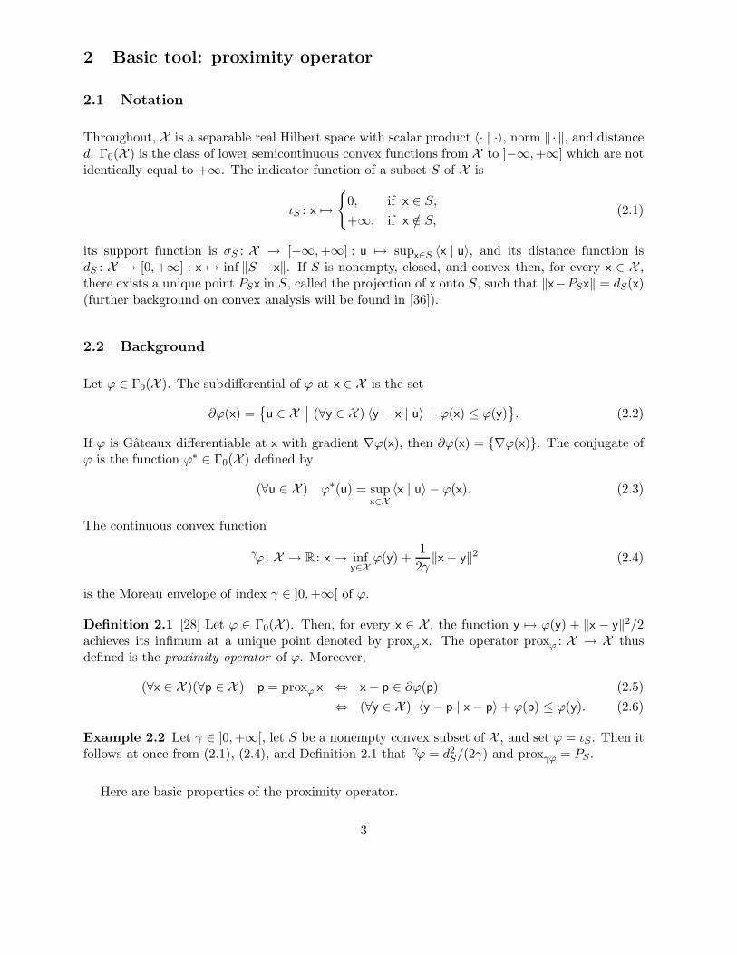
As discussed in Section 3.3.2, the functions (φk)k∈K in (3.2) act as the potential functions of log-concave univariate probability densities modeling the frame coefficients individually in Bayesianformulations. On the other hand, the proximity operators of such functions will, via Proposi-tion 2.10, play a central role in Section 5. Hereafter, we derive closed-form expressions for theseproximity operators in the case of some classical log-concave univariate probability densities [19,Chapters VII&IX].

Let us start with a few observations.

Remark 4.1 Let φ ∈ Γ0(R).

(i) It follows from Definition 2.1 that (∀ξ ∈ R) φ(proxφ ξ) < +∞.

13

(ii) If φ is even, then it follows from Lemma 2.5(iv) that proxφ is odd. Therefore, in suchinstances, it will be enough to determine proxφ ξ for ξ ≥ 0 and to extend the result to ξ < 0by antisymmetry.

(iii) Let ξ ∈ R. If φ is differentiable at proxφ ξ, then (2.5) yields

(∀π ∈ R) π = proxφ ξ ⇔ π + φ′(π) = ξ. (4.1)

We now examine some concrete examples.

Example 4.2 (Laplace distribution) Let ω ∈ ]0,+∞[ and set

φ : R → ]−∞,+∞] : ξ 7→ ω|ξ|. (4.2)

Then, for every ξ ∈ R, proxφ ξ = soft[−ω,ω] ξ = sign(ξ)max|ξ| − ω, 0.

Proof. Apply Lemma 2.6(iii) with ψ = 0 and Ω = [−ω, ω].

Example 4.3 (Gaussian distribution) Let τ ∈ ]0,+∞[ and set

φ : R → ]−∞,+∞] : ξ 7→ τ |ξ|2. (4.3)

Then, for every ξ ∈ R, proxφ ξ = ξ/(2τ + 1).

Proof. Apply Lemma 2.5(i) with X = R, ϕ = 0, α = 2τ , and u = 0.

Example 4.4 (generalized Gaussian distribution) Let p ∈ ]1,+∞[, κ ∈ ]0,+∞[, and set

φ : R → ]−∞,+∞] : ξ 7→ κ|ξ|p. (4.4)

Then, for every ξ ∈ R, proxφ ξ = sign(ξ) where is the unique solution in [0,+∞[ to

+ pκp−1 = |ξ|. (4.5)

In particular, the following hold:

(i) proxφ ξ = ξ +4κ

3 · 21/3

(

(χ− ξ)1/3 − (χ+ ξ)1/3)

, where χ =√

ξ2 + 256κ3/729, if p = 4/3;

(ii) proxφ ξ = ξ + 9κ2 sign(ξ)(

1 −√

1 + 16|ξ|/(9κ2))

/8, if p = 3/2;

(iii) proxφ ξ = sign(ξ)(√

1 + 12κ|ξ| − 1)

/(6κ), if p = 3;

(iv) proxφ ξ =

(

χ+ ξ

8κ

)1/3

−(

χ− ξ

8κ

)1/3

, where χ =√

ξ2 + 1/(27κ), if p = 4.

14

Proof. Let ξ ∈ R and set π = proxφ ξ. As seen in Remark 4.1(ii), because φ is even, it is enoughto assume that ξ ≥ 0. Since φ is differentiable, it follows from (2.7) and (4.1) that π is the uniquesolution in [0,+∞[ to

π + pκπp−1 = ξ, (4.6)

which provides (4.5). For p = 3, π is the solution in [0,+∞[ to the equation π + 3κπ2 − ξ = 0,i.e., π = (

√1 + 12κξ − 1)/(6κ) and we obtain (iii) by antisymmetry. In turn, since

(

2| · |3/2/3)∗

=| · |3/3, Lemma 2.3(iii) with γ = 3κ/2 yields π = proxγ(2|·|3/2/3) ξ = ξ − γ prox(3γ)−1|·|3(ξ/γ) =

ξ + 9κ2 sign(ξ)(

1 −√

1 + 16|ξ|/(9κ2))

/8, which proves (ii). Now, let p = 4. Then (4.6) assertsthat π is the unique solution in [0,+∞[ to the third degree equation 4κπ3 + π − ξ = 0, namely

π =(√

α2 + β3 − α)1/3 −

(√

α2 + β3 + α)1/3

, where α = −ξ/(8κ) and β = 1/(12κ). Since thisexpression is an odd function of ξ, we obtain (iv). Finally, we deduce (i) from (iv) by observingthat, since

(

3| · |4/3/4)∗

= | · |4/4, Lemma 2.3(iii) with γ = 4κ/3 yields π = proxγ(3|·|4/3/4) ξ =ξ − γ prox(4γ)−1|·|4(ξ/γ), hence the result after simple algebra.

Example 4.5 (Huber distribution) Let ω ∈ ]0,+∞[, τ ∈ ]0,+∞[, and set

φ : R → ]−∞,+∞] : ξ 7→

τξ2, if |ξ| ≤ ω/√

2τ ;

ω√

2τ |ξ| − ω2/2, otherwise.(4.7)

Then, for every ξ ∈ R,

proxφ ξ =

ξ

2τ + 1, if |ξ| ≤ ω(2τ + 1)/

√2τ ;

ξ − ω√

2τ sign(ξ), if |ξ| > ω(2τ + 1)/√

2τ .

(4.8)

Proof. Let ξ ∈ R and set π = proxφ ξ. Since φ is even, we assume that ξ ≥ 0 (see Remark 4.1(ii)).In addition, since φ is differentiable, it follows from (2.7) and (4.1) that π is the unique solutionin [0, ξ] to π + φ′(π) = ξ. First, suppose that π = ω/

√2τ . Then φ′(π) = ω

√2τ and, therefore,

ξ = π + φ′(π) = ω(2τ + 1)/√

2τ . Now, suppose that ξ ≤ ω(2τ + 1)/√

2τ . Then it follows fromLemma 2.6(i) that π ≤ proxφ(ω(2τ +1)/

√2τ) = ω/

√2τ . In turn, (4.7) yields φ′(π) = 2τπ and the

identity ξ = π + φ′(π) yields π = ξ/(2τ + 1). Finally, if ξ > ω(2τ + 1)/√

2τ , then Lemma 2.6(i)yields π ≥ proxφ(ω(2τ + 1)/

√2τ) = ω/

√2τ and, in turn, φ′(π) = ω

√2τ , which allows us to

conclude that π = ξ − ω√

2τ .

Example 4.6 (maximum entropy distribution) This density is obtained by maximizing theentropy subject to the knowledge of the first, second, and p-th order absolute moments, where2 6= p ∈ ]1,+∞[ [24]. Let ω ∈ ]0,+∞[, τ ∈ [0,+∞[, κ ∈ ]0,+∞[, and set

φ : R → ]−∞,+∞] : ξ 7→ ω|ξ| + τ |ξ|2 + κ|ξ|p. (4.9)

Then, for every ξ ∈ R,

proxφ ξ = sign(ξ) proxκ|·|p/(2τ+1)

( 1

2τ + 1max|ξ| − ω, 0

)

(4.10)

where the expression of proxκ|·|p/(2τ+1) is supplied by Example 4.4.

15

Proof. The function φ is a quadratic perturbation of the function ϕ = ω| · | + κ| · |p. ApplyingLemma 2.6(iii) with ψ = κ| · |p and Ω = [−ω, ω], we get (∀ξ ∈ R) proxϕ ξ = proxκ|·|p(soft[−ω,ω] ξ) =sign(ξ) proxκ|·|p(max|ξ| − ω, 0). Hence, the result follows from Lemma 2.5(i) where X = R,α = 2τ , and u = 0.

Example 4.7 (smoothed Laplace distribution) Let ω ∈ ]0,+∞[ and set

φ : R → ]−∞,+∞] : ξ 7→ ω|ξ| − ln(1 + ω|ξ|). (4.11)

This potential function is sometimes used as a differentiable approximation to (4.2), e.g., [29]. Wehave, for every ξ ∈ R,

proxφ ξ = sign(ξ)ω|ξ| − ω2 − 1 +

√

∣

∣ω|ξ| − ω2 − 1∣

∣

2+ 4ω|ξ|

2ω. (4.12)

Proof. According to Remark 4.1(ii), since φ is even, we can focus on the case when ξ ≥ 0. As φachieves its infimum at 0, Lemma 2.6(ii) yields π = proxφ ξ ≥ 0. We deduce from (4.1) that π isthe unique solution in [0,+∞[ to the equation

ωπ2 + (ω2 + 1 − ωξ)π − ξ = 0, (4.13)

which leads to (4.12).

Example 4.8 (exponential distribution) Let ω ∈ ]0,+∞[ and set

φ : R → ]−∞,+∞] : ξ 7→

ωξ, if ξ ≥ 0;

+∞, if ξ < 0.(4.14)

Then, for every ξ ∈ R,

proxφ ξ =

ξ − ω if ξ ≥ ω;

0 if ξ < ω.(4.15)

Proof. Set ϕ = ι[0,+∞[. Then Example 2.2 yields proxϕ = P[0,+∞[. In turn, since φ is a linearperturbation of ϕ, the claim results from Lemma 2.5(i), where X = R, α = 0, and u = ω.

Example 4.9 (gamma distribution) Let ω ∈ ]0,+∞[, κ ∈ ]0,+∞[, and set

φ : R → ]−∞,+∞] : ξ 7→

−κ ln(ξ) + ωξ, if ξ > 0;

+∞, if ξ ≤ 0.(4.16)

Then, for every ξ ∈ R,

proxφ ξ =ξ − ω +

√

|ξ − ω|2 + 4κ

2. (4.17)

16

Proof. Set

ϕ : R → ]−∞,+∞] : ξ 7→

−κ ln(ξ), if ξ > 0;

+∞, if ξ ≤ 0.(4.18)

We easily get from Remark 4.1(i)&(iii) that

(∀ξ ∈ R) proxϕ ξ =ξ +

√

ξ2 + 4κ

2. (4.19)

In turn, since φ is a linear perturbation of ϕ, the claim results from Lemma 2.5(i), where X = R,α = 0, and u = ω.

Example 4.10 (chi distribution) Let κ ∈ ]0,+∞[ and let

φ : R → ]−∞,+∞] : ξ 7→

−κ ln(ξ) + ξ2/2, if ξ > 0;

+∞, if ξ ≤ 0.(4.20)

Then, for every ξ ∈ R,

proxφ ξ =ξ +

√

ξ2 + 8κ

4. (4.21)

Proof. Since φ is a quadratic perturbation of the function ϕ defined in (4.18), the claim resultsfrom Lemma 2.5(i), where X = R, α = 1, and u = 0.

Example 4.11 (uniform distribution) Let ω ∈ ]0,+∞[ and set φ = ι[−ω,ω]. Then it follows atonce from Example 2.2 that, for every ξ ∈ R,

proxφ ξ = P[−ω,ω]ξ =

−ω, if ξ < −ω;

ξ, if |ξ| ≤ ω;

ω, if ξ > ω.

(4.22)

Example 4.12 (triangular distribution) Let ω ∈ ]−∞, 0[, let ω ∈ ]0,+∞[, and set

φ : R → ]−∞,+∞] : ξ 7→

− ln(ξ − ω) + ln(−ω), if ξ ∈ ]ω, 0] ;

− ln(ω − ξ) + ln(ω), if ξ ∈ ]0, ω[ ;

+∞, otherwise.

(4.23)

Then, for every ξ ∈ R,

proxφ ξ =

ξ + ω +√

|ξ − ω|2 + 4

2, if ξ < 1/ω;

ξ + ω −√

|ξ − ω|2 + 4

2, if ξ > 1/ω;

0 otherwise.

(4.24)

17

Proof. Let ξ ∈ R and set π = proxφ ξ. Let us first note that ∂φ(0) = [1/ω, 1/ω]. Therefore, (2.5)yields

π = 0 ⇔ ξ ∈ [1/ω, 1/ω] . (4.25)

Now consider the case when ξ > 1/ω. Since φ admits 0 as a minimizer, it follows from Lemma 2.6(ii)and (4.25) that π ∈ ]0, ξ]. Hence, we derive from (4.1) that π is the only solution in ]0, ξ] toπ + 1/(ω − π) = ξ, i.e., π = (ξ + ω −

√

|ξ − ω|2 + 4)/2. Likewise, if ξ < 1/ω, it follows fromLemma 2.6(ii), (4.25), and (4.1) that π is the only solution in [ξ, 0[ to π − 1/(π − ω) = ξ, whichyields π = (ξ + ω +

√

|ξ − ω|2 + 4)/2.

The next example is an extension of Example 4.10.

Example 4.13 (Weibull distribution) Let ω ∈ ]0,+∞[, κ ∈ ]0,+∞[, and p ∈ ]1,+∞[, and set

φ : R → ]−∞,+∞] : ξ 7→

−κ ln(ξ) + ωξp, if ξ > 0;

+∞, if ξ ≤ 0.(4.26)

Then, for every ξ ∈ R, π = proxφ ξ is the unique strictly positive solution to

pωπp + π2 − ξπ = κ. (4.27)

Proof. Since φ is differentiable on ]0,+∞[, it follows from Remark 4.1(i)&(iii) that π is the uniquesolution in ]0,+∞[ to π + φ′(π) = ξ or, equivalently, to (4.27).

A similar proof can be used in the following two examples.

Example 4.14 (generalized inverse Gaussian distribution) Let ω ∈ ]0,+∞[, κ ∈ [0,+∞[,and ρ ∈ ]0,+∞[, and set

φ : R → ]−∞,+∞] : ξ 7→

−κ ln(ξ) + ωξ + ρ/ξ, if ξ > 0;

+∞, if ξ ≤ 0.(4.28)

Then, for every ξ ∈ R, π = proxφ ξ is the unique strictly positive solution to

π3 + (ω − ξ)π2 − κπ = ρ. (4.29)

Example 4.15 (Pearson type I) Let κ and κ be in ]0,+∞[, let ω and ω be reals such thatω < ω, and set

φ : R → ]−∞,+∞] : ξ 7→

−κ ln(ξ − ω) − κ ln(ω − ξ), if ξ ∈ ]ω, ω[ ;

+∞, otherwise.(4.30)

Then, for every ξ ∈ R, π = proxφ ξ is the unique solution in ]ω, ω[ to

π3 − (ω + ω + ξ)π2 +(

ωω − κ− κ+ (ω + ω)ξ)

π = ωωξ − ωκ− ωκ. (4.31)

Remark 4.16

18

(i) The chi-square distribution with n > 2 degrees of freedom is a special case of the gammadistribution (Example 4.9) with (ω, κ) = (1/2, n/2 − 1).

(ii) The normalized Rayleigh distribution is a special case of the chi distribution (Example 4.10)with κ = 1.

(iii) The beta distribution and the Wigner distribution are special cases of the Pearson type Idistribution (Example 4.15) with (ω, ω) = (0, 1), and −ω = ω and κ = κ = 1/2, respectively.

(iv) The proximity operator associated with translated and/or scaled versions of the above den-sities can be obtained via Lemma 2.5(ii)&(iii).

(v) For log-concave densities for which the proximity operator of the potential function is difficultto express in closed form (e.g., Kumaraswamy or logarithmic distributions), one can turn tosimple procedures to solve (2.5) or (4.1) numerically.

5 Algorithm

We propose the following algorithm to solve Problem 3.1.

Algorithm 5.1 Fix x0 ∈ ℓ2(K) and construct a sequence (xn)n∈N = ((ξn,k)k∈K)n∈N by setting, forevery n ∈ N,

(∀k ∈ K) ξn+1,k = ξn,k + λn

(

proxγnφk

(

ξn,k − γn(ηn,k + βn,k))

+ αn,k − ξn,k

)

, (5.1)

where λn ∈ ]0, 1], γn ∈ ]0,+∞[, αn,kk∈K ⊂ R, (ηn,k)k∈K = F (∇Ψ(F ∗xn)), and (βn,k)k∈K = Fbn,where bn ∈ H.

The chief advantage of this algorithm is to be fully split in the sense that the functions (φk)k∈K

and Ψ appearing in (3.2) are used separately. First, the current iterate xn is transformed into a pointin F ∗xn in H, and the gradient of Ψ is evaluated at this point to within some tolerance bn. Next, weobtain the sequence (ηn,k)k∈K = F (∇Ψ(F ∗xn)) to within some tolerance (βn,k)k∈K = Fbn. Thenone chooses γn > 0, and, for every k ∈ K, applies the operator proxγnφk

to ξn,k−γn(ηn,k+βn,k). Anerror αn,k is tolerated in this computation. Finally, the kth component ξn+1,k of xn+1 is obtainedby applying a relaxation of parameter λn to this inexact proximal step. Let us note that thecomputation of the proximal steps can be performed in parallel.

To study the asymptotic behavior of the sequences generated by Algorithm 5.1, we require thefollowing set of assumptions.

Assumption 5.2 In addition to the standing assumptions of Problem 3.1, the following hold.

(i) Problem 3.1 admits a solution.

(ii) infn∈N λn > 0.

19

(iii) infn∈N γn > 0 and supn∈N γn < 2/β, where β is a Lipschitz constant of F ∇Ψ F ∗.

(iv)∑

n∈N

√∑

k∈K|αn,k|2 < +∞ and

∑

n∈N‖bn‖ < +∞.

Remark 5.3 As regards Assumption 5.2(i), sufficient conditions can be found in Proposition 3.3.Let us now turn to the parameter β in Assumption 5.2(iii), which determines the range of the stepsizes (γn)n∈N. It follows from the assumptions of Problem 3.1 and (1.1) that, for every x and y inℓ2(K),

‖F (∇Ψ(F ∗x)) − F (∇Ψ(F ∗y))‖ ≤ ‖F‖ ‖∇Ψ(F ∗x) −∇Ψ(F ∗y)‖≤ τ‖F‖ ‖F ∗x − F ∗y‖≤ τ‖F‖2 ‖x − y‖≤ τν‖x − y‖. (5.2)

Thus, the value β = τν can be used in general. In some cases, however, a sharper bound can beobtained, which results in a wider range for the step sizes (γn)n∈N. For example, in the problemconsidered in Section 3.3.1, if the norm of R =

∑qi=1 αiFT

∗i TiF

∗ can be evaluated, it follows from(3.13) and the nonexpansivity of the operators (Id −PSi)1≤i≤m that one can take

β = ‖R‖ + ν

m∑

i=1

ϑi. (5.3)

Theorem 5.4 Let (xn)n∈N be an arbitrary sequence generated by Algorithm 5.1 under Assump-

tion 5.2. Then (xn)n∈N converges weakly to a solution to Problem 3.1.

Proof. Set X = ℓ2(K), f1 =∑

k∈Kφk(〈· | ok〉), and f2 = Ψ F ∗, where (ok)k∈K denotes the

canonical orthonormal basis of ℓ2(K). Then ∇f2 = F ∇Ψ F ∗ is β-Lipschitz continuous (seeAssumption 5.2(iii)) and, as seen in the proof of Proposition 3.4, (3.2) conforms to the format ofProblem 2.7. Furthermore, it follows from Proposition 2.10 that we can rewrite (5.1) as

xn+1 = xn + λn

(

∑

k∈K

(

proxγnφk〈xn − γnF (∇Ψ(F ∗xn) + bn) | ok〉 + αn,k

)

ok − xn

)

= xn + λn

(

proxγnf1

(

xn − γn(∇f2(xn) + bn))

+ an − xn

)

, (5.4)

where an = (αn,k)k∈K and bn = Fbn. Since Assumption 5.2(iv) and (1.1) imply that∑

n∈N‖an‖ <

+∞ and∑

n∈N‖bn‖ ≤ √

ν∑

n∈N‖bn‖ < +∞, the claim therefore follows from Theorem 2.9.

Let (xn)n∈N be a sequence generated by Algorithm 5.1 under Assumption 5.2 and set (∀n ∈ N)xn = F ∗xn. On the one hand, Theorem 5.4 asserts that (xn)n∈N converges weakly to a solutionx to Problem 3.1. On the other hand, since F ∗ is linear and bounded, it is weakly continuousand, therefore, (xn)n∈N converges weakly to F ∗x. However, it is not possible to express (5.1) as aniteration in terms of the sequence (xn)n∈N in H in general. The following corollary addresses thecase when F is surjective, which does lead to an algorithm in H.

20

Corollary 5.5 Suppose that (ek)k∈K is a Riesz basis with companion biorthogonal basis (ek)k∈K.

Fix x0 ∈ H and, for every n ∈ N, set

xn+1 = xn + λn

(

∑

k∈K

(

proxγnφk

(

〈xn | ek〉 − γn〈∇Ψ(xn) + bn | ek〉)

+ αn,k)

ek − xn

)

, (5.5)

where λn ∈ ]0, 1], γn ∈ ]0,+∞[, αn,kk∈K ⊂ R, and bn ∈ H. Suppose that Assumption 5.2

is in force. Then (xn)n∈N converges weakly to a point x ∈ H and (〈x | ek〉)k∈K is a solution to

Problem 3.1.

Proof. Set (∀n ∈ N)(∀k ∈ K) ξn,k = 〈xn | ek〉, ηn,k = 〈∇Ψ(xn) | ek〉, and βn,k = 〈bn | ek〉. Then,for every n ∈ N, it follows from (1.4) that xn = F ∗(ξn,k)k∈K and, in turn, that

(ηn,k)k∈K = F (∇Ψ(F ∗xn)), where xn = (ξn,k)k∈K. (5.6)

Furthermore, for every n ∈ N, it follows from (5.5) and the biorthogonality of (ek)k∈K and (ek)k∈K

that

(∀k ∈ K) ξn+1,k = 〈xn+1 | ek〉

= 〈xn | ek〉 + λn

(

proxγnφk

(

〈xn | ek〉 − γn〈∇Ψ(xn) + bn | ek〉)

+ αn,k

− 〈xn | ek〉)

= ξn,k + λn

(

proxγnφk

(

ξn,k − γn(ηn,k + βn,k))

+ αn,k − ξn,k

)

. (5.7)

Since Theorem 5.4 states that (xn)n∈N converges weakly to a solution x to Problem 3.1, (xn)n∈N =(F ∗xn)n∈N converges weakly to x = F ∗x. Consequently, (1.4) asserts that we can write x =(〈x | ek〉)k∈K.

Remark 5.6 Suppose that K = N and that (ek)k∈K is an orthonormal basis of H. Then (5.5)reduces to

xn+1 = xn + λn

(

∑

k∈K

(

proxγnφk

(

〈xn − γn(∇Ψ(xn) + bn) | ek〉)

+ αn,k)

ek − xn

)

. (5.8)

In this particular setting, some results related to Corollary 5.5 are the following.

(i) Suppose that Ψ: x 7→ ‖Tx − z‖2/2, where T is a nonzero bounded linear operator from Hto a real Hilbert space G and z ∈ G. Suppose that, in addition, (∀k ∈ K) φk ≥ φk(0) = 0.Then the convergence of (5.8) is discussed in [15, Corollary 5.16].

(ii) Suppose that (Ωk)k∈K are closed intervals of R such that 0 ∈ int⋂

k∈KΩk and that

(∀k ∈ K) φk = ψk + σΩk, (5.9)

where ψk ∈ Γ0(R) is differentiable at 0 and ψk ≥ ψk(0) = 0. Then (5.8) is the thresholdingalgorithm proposed and analyzed in [14], namely

xn+1 = xn + λn

(

∑

k∈K

(

proxγnψk

(

softγnΩk〈xn − γn(∇Ψ(xn) + bn) | ek〉

)

+ αn,k

)

ek − xn

)

,

(5.10)where softγnΩk

is defined in (2.8).

21

(iii) Suppose that the assumptions of both (i) and (ii) hold and that, in addition, we set λn ≡ 1,‖T‖ < 1, γn ≡ 1, αn,k ≡ 0, bn ≡ 0, and (∀k ∈ K) ψk = 0 and Ωk = [−ωk, ωk]. Then (5.10)becomes

xn+1 =∑

k∈K

(

soft[−ωk,ωk] 〈xn + T ∗(z − Txn) | ek〉)

ek. (5.11)

Algorithm 5.1 can be regarded as a descendant of this original method, which is investigatedin [17] and [18].

6 Numerical results

The proposed framework is applicable to a wide array of variational formulations for inverse prob-lems over frames. We provide a couple of examples to illustrate its applicability in wavelet-basedimage restoration in the Euclidean space H = R512×512. The choice of the potential functions(φk)k∈K in Problem 3.1 is guided by the observation that regular images typically possess sparsewavelet representations and that the resulting wavelet coefficients often have even probability den-sity functions [26]. Among the candidate potential functions investigated in Section 4, those ofExample 4.6 appear to be the most appropriate for modeling wavelet coefficients on two counts.First, they provide flexible models of even potentials. Second, as shown in Lemma 2.6(iii), theirproximity operators are thresholders and they therefore promote sparsity. More precisely, we em-ploy potential functions of the form φk = ωk| · | + τk| · |2 + κk| · |pk , where pk ∈ 4/3, 3/2, 3, 4and ωk, τk, κk ⊂ ]0,+∞[. Note that proxφk

can be obtained explicitly via (4.10) and Exam-ples 4.4(i)-(iv). In addition, it follows from Proposition 3.3(iii)(b) that, with such potential func-tions, Problem 3.1 does admit a solution. The values of the parameters ωk, τk, κk, and pk arechosen for each wavelet subband via a maximum likelihood approach. The first example uses abiorthogonal wavelet basis and the second one uses an M -band dual-tree wavelet frame. Let usemphasize that such decompositions cannot be dealt with using the methods developed in [14],which are limited to orthonormal basis representations. Algorithm 5.1 is implemented with λn ≡ 1and large step sizes (i.e., γn close to 2/β) since such values have been observed to provide a goodspeed of convergence in our experiments.

6.1 Example 1

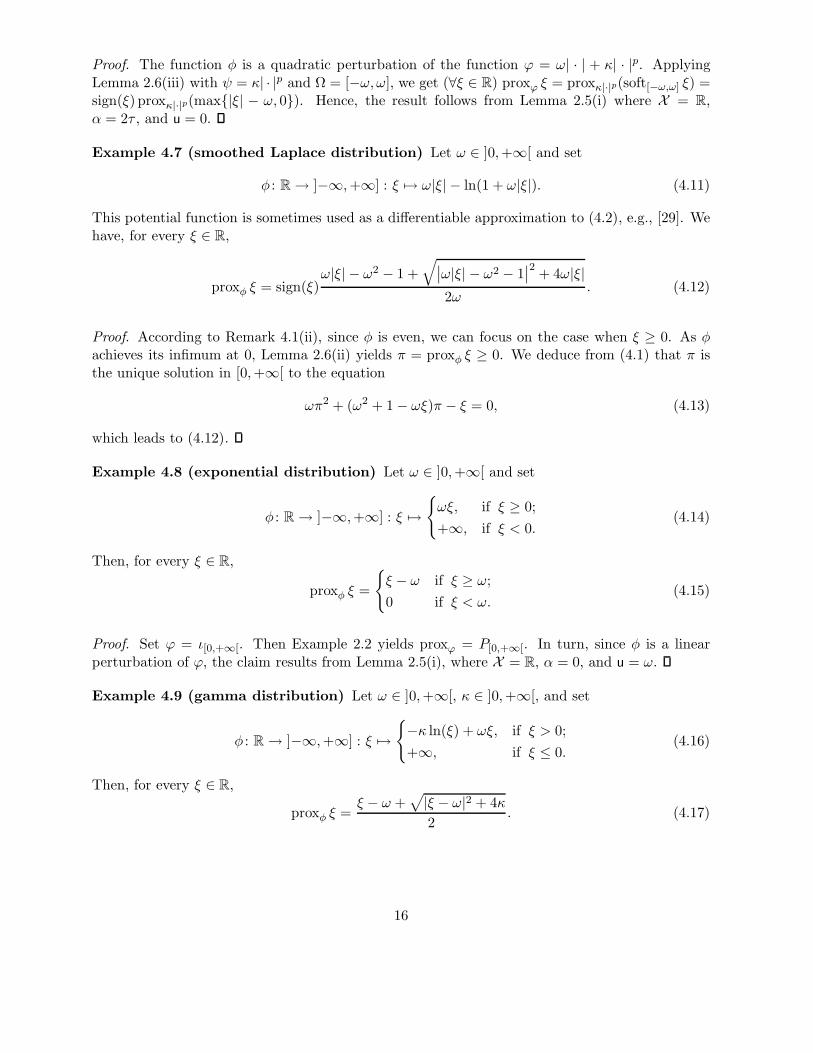
We provide a multiview restoration example in a biorthogonal wavelet basis. The original image xis the standard test image displayed in Fig. 2 (top left). Two observations (see Fig. 2 top right andbottom left) conforming to the model (3.12) are available. In our experiment, G1 = G2 = H and v1and v2 are realizations of two independent zero-mean Gaussian white noise processes. Moreover,the operator T1 models a motion blur in the diagonal direction and satisfies ‖T1‖ = 1, whereasT2 = Id /2. The blurred image-to-noise ratio is higher for the first observation (22.79 dB versus15.18 dB) and so is the relative error (18.53 dB versus 5.891 dB) (the decibel value of the relativeerror between an image z and x is 20 log10 (‖x‖/‖z − x‖)). The function Ψ in Problem 3.1 is givenby (3.13), where α1 = 4.00×10−2 and α2 = 6.94×10−3 are the inverses of the variances of the noisecorrupting each observation. In addition, we set m = 1, ϑ1 = 10−2, and S1 = [0, 255]512×512 toenforce the known range of the pixel values. A discrete biorthogonal spline 9-7 decomposition [2] is

22

used over 3 resolution levels. Algorithm 5.1 is used to solve Problem 3.1. By numerically evaluating‖R‖ in (5.3), we obtain β = 0.230 and the step sizes are chosen to be γn ≡ 1.99/β = 8.66. Theresulting restored image, shown in Fig. 2 (bottom right), yields a relative error of 23.84 dB.

6.2 Example 2

The original SPOT5 satellite image x is shown in Fig. 3 (top) and the degraded image z in G = His shown in Fig. 3 (center). The degradation model is given by (3.16), where T is a 7 × 7 uniformblur with ‖T‖ = 1, and where v is a realization of a zero-mean Gaussian white noise process. Theblurred image-to-noise ratio is 28.08 dB and the relative error is 12.49 dB.

In this example, we perform a restoration in a discrete two-dimensional version of an M -banddual-tree wavelet frame [7]. This decomposition has a redundancy factor of 2 (i.e., with thenotation of Section 3.3.2, K/N = 2). In our experiments, decompositions over 2 resolution levelsare performed with M = 4 using the filter bank proposed in [1]. The function Ψ in Problem 3.1 isgiven by (3.22), where fV is the probability density function of the Gaussian noise. A solution isobtained via Algorithm 5.1. For the representation under consideration, we derive from (5.3) thatβ = 2 and we set γn ≡ 0.995. The restored image, shown in Fig. 3 (bottom), yields a relative errorof 15.68 dB, i.e., a significant improvement of over 3 dB in terms of signal-to-noise ratio. A moreprecise inspection of the magnified areas displayed in Fig. 4 shows that the proposed method makesit possible to recover sharp edges while removing noise in uniform areas. This behavior in termsof edge recovery may be attributed to the choice of the M -band dual-tree wavelet decomposition,which is known to provide a good representation of directional features such as edges [7].

References

[1] O. Alkin and H. Caglar, Design of efficient M -band coders with linear-phase and perfect-reconstructionproperties, IEEE Trans. Signal Process., vol. 43, pp. 1579–1590, 1995.

[2] M. Antonini, M. Barlaud, P. Mathieu, and I. Daubechies, Image coding using wavelet transform, IEEE

Trans. Image Process., vol. 1, pp. 205–220, 1992.

[3] J. M. Bioucas-Dias, Bayesian wavelet-based image deconvolution: a GEM algorithm exploiting a classof heavy-tailed priors, IEEE Trans. Image Process., vol. 15, pp. 937–951, 2006.

[4] C. Bouman and K. Sauer, A generalized Gaussian image model for edge-preserving MAP estimation,IEEE Trans. Image Process., vol. 2, pp. 296–310, 1993.

[5] C. L. Byrne, A unified treatment of some iterative algorithms in signal processing and image recon-struction, Inverse Problems, vol. 20, pp. 103–120, 2004.

[6] E. J. Candes and D. L. Donoho, Recovering edges in ill-posed inverse problems: Optimality of curveletframes, Ann. Statist., vol. 30, pp. 784–842, 2002.

[7] C. Chaux, L. Duval, and J.-C. Pesquet, Image analysis using a dual-tree M -band wavelet transform,IEEE Trans. Image Process., vol. 15, pp. 2397–2412, 2006.

[8] A. Cohen, Numerical Analysis of Wavelet Methods. Elsevier, New York, 2003.

23

[9] A. Cohen, I. Daubechies, and J.-C. Feauveau, Biorthogonal bases of compactly supported wavelets,Comm. Pure Appl. Math., vol. 45, pp. 485–560, 1992.

[10] P. L. Combettes, The foundations of set theoretic estimation, Proc. IEEE, vol. 81, pp. 182–208, 1993.

[11] P. L. Combettes, Inconsistent signal feasibility problems: Least-squares solutions in a product space,IEEE Trans. Signal Process., vol. 42, pp. 2955–2966, 1994.

[12] P. L. Combettes, A block-iterative surrogate constraint splitting method for quadratic signal recovery,IEEE Trans. Signal Process., vol. 51, pp. 1771–1782, 2003.

[13] P. L. Combettes, Solving monotone inclusions via compositions of nonexpansive averaged operators,Optimization, vol. 53, pp. 475–504, 2004.

[14] P. L. Combettes and J.-C. Pesquet, Proximal thresholding algorithm for minimization over orthonormalbases, SIAM J. Optim., to appear.

[15] P. L. Combettes and V. R. Wajs, Signal recovery by proximal forward-backward splitting, Multiscale

Model. Simul., vol. 4, pp. 1168–1200, 2005.

[16] I. Daubechies, Ten Lectures on Wavelets. SIAM, Philadelphia, PA, 1992.

[17] I. Daubechies, M. Defrise, and C. De Mol, An iterative thresholding algorithm for linear inverseproblems with a sparsity constraint, Comm. Pure Appl. Math., vol. 57, pp. 1413–1457, 2004.

[18] C. de Mol and M. Defrise, A note on wavelet-based inversion algorithms, Contemp. Math., vol. 313,pp. 85–96, 2002.

[19] L. Devroye, Non-Uniform Random Variate Generation. Springer-Verlag, New York, 1986.

[20] M. N. Do and M. Vetterli, The contourlet transform: An efficient directional multiresolution imagerepresentation, IEEE Trans. Image Process., vol. 14, pp. 2091–2106, 2005.

[21] M. Elad and A. Feuer, Restoration of a single superresolution image from several blurred, noisy, andundersampled measured images, IEEE Trans. Image Process., vol. 6, pp. 1646–1658, 1997.

[22] O. D. Escoda, L. Granai, and P. Vandergheynst, On the use of a priori information for sparse signalapproximations, IEEE Trans. Signal Process., vol. 54, pp. 3468–3482, 2006.

[23] D. Han and D. R. Larson, Frames, Bases, and Group Representations. Mem. Amer. Math. Soc., vol.147, 2000.

[24] J. N. Kapur and H. K. Kesevan, Entropy Optimization Principles with Applications. Academic Press,Boston, 1992.

[25] E. Le Pennec and S. G. Mallat, Sparse geometric image representations with bandelets, IEEE Trans.

Image Process., vol. 14, pp. 423–438, 2005.

[26] S. G. Mallat, A Wavelet Tour of Signal Processing, 2nd ed. Academic Press, New York, 1999.

[27] J.-J. Moreau, Fonctions convexes duales et points proximaux dans un espace hilbertien, C. R. Acad.

Sci. Paris Ser. A Math., vol. 255, pp. 2897–2899, 1962.

[28] J.-J. Moreau, Proximite et dualite dans un espace hilbertien, Bull. Soc. Math. France, vol. 93, pp.273-299, 1965.

24

−5 −4 −3 −2 −1 1 2 3 4 5

−4

−3

−2

−1

1

2

3

4

Figure 1: Ω = [−1, 1]. Graphs of softΩ (dashed line) and proxφ (solid line) in Lemma 2.6(iii) withψ = 0.1| · |3.

[29] M. Nikolova and M. K. Ng, Analysis of half-quadratic minimization methods for signal and imagerecovery, SIAM J. Sci. Comput., vol. 27, pp. 937–966, 2005.

[30] I. W. Selesnick, R. G. Baraniuk, and N. C. Kingsbury, The dual-tree complex wavelet transform, IEEE

Signal Process. Mag., vol. 22, pp. 123–151, 2005.

[31] H. Stark, ed., Image Recovery: Theory and Application. Academic Press, San Diego, CA, 1987.

[32] A. M. Thompson and J. Kay, On some Bayesian choices of regularization parameter in image restora-tion, Inverse Problems, vol. 9, pp. 749–761, 1993.

[33] R. Tolimieri and M. An, Time-Frequency Representations. Birkhauser, Boston, MA, 1998.

[34] J. A. Tropp, Just relax: Convex programming methods for identifying sparse signals in noise, IEEE

Trans. Inform. Theory, vol. 52, pp. 1030–1051, 2006.

[35] H. L. Van Trees, Detection, Estimation, and Modulation Theory – Part I. Wiley, New York, 1968.

[36] C. Zalinescu, Convex Analysis in General Vector Spaces. World Scientific, River Edge, NJ, 2002.

25

Figure 2: Example 1 – Original image (top left), first observation (top right), second observation(bottom left), and image restored with 200 iterations of Algorithm 5.1 (bottom right).

26

Figure 3: Example 2 – Original image (top); degraded image (center); image restored in a dual-treewavelet frame with 100 iterations of Algorithm 5.1 (bottom).

27

Figure 4: Example 2 – Zoom on a 100× 100 portion of the SPOT5 satellite image. Original image(top); degraded image (center); image restored in a dual-tree wavelet frame with 100 iterations ofAlgorithm 5.1 (bottom).

28