FINAL REPORT SUBMITTED TO

THE NATIONAL SCIENCE FOUNDATION, WASHINGTON, D. C. FOR

GRANT: OCE 10-38891 CLIMATOLOGICAL MEAN DISTRIBUTION OF pH AND CARBONATE ION CONCENTRATION IN GLOBAL OCEAN SURFACE WATERS IN THE UNIFIED pH SCALE AND MEAN RATE OF THIER CHANGES IN SELECTED AREAS

by Taro Takahashi and Stewart C. Sutherland

Lamont-Doherty Earth Observatory of Columbia University Palisades, NY 10964

(January 8, 2013) ABSTRACT Climatological mean monthly distribution of pH and the degree of aragonite saturation have been determined for the surface water of the global oceans using a data set for pCO2, TCO2, alkalinity and nutrient concentrations in surface waters (depths <50 m), which is built upon the GLODAP, CARINA and LDEO database. The mutual consistency among these parameters is demonstrated using the inorganic carbon chemistry model. The global ocean is divided into 33 regions, and the potential alkalinity-salinity relationships (linear regressions) in 32 of these regions (excluding the equatorial Pacific El Nino zone) are established. Using the mean monthly pCO2 data adjusted to a reference year 2005 and the alkalinity estimated using the potential alkalinity-salinity relationships, the mean monthly distributions of pH and aragonite saturation in surface ocean waters are obtained for the year 2005. The pH in the global ocean surface waters ranges from 7.9 to 8.2 in the year 2005. Lower values are located in the upwelling regions in the equatorial Pacific and in the Arabian and Bering Seas; and higher values are found in the subpolar and polar waters during the spring-summer months of intense photosynthetic production. The vast areas of subtropical oceans have seasonally varying pH values ranging from 8.05 during warmer months to 8.15 during colder months. The warm tropical and subtropical waters are supersaturated by a factor of as much as 4.2 with respect to aragonite and 6.3 for calcite, whereas the cold subpolar and polar waters are less supersaturated only by a factor of 1.2 for aragonite and 2 for calcite because of the lower pH values resulting from greater TCO2 concentration. In the western Arctic Ocean, aragonite undersaturation is observed. Decadal time-series data at the Bermuda (BATS), Hawaii (HOT) and Drake Passage show that pH has been declining at a mean rate of about 0.002 per year. INTRODUCTION

Most active biological production takes place in the sun-lit top layer of the global ocean. Yet, this is the layer that is being acidified as a result of the absorption of rapidly increasing CO2 from the atmosphere. Marine ecosystems in general will be influenced by changes in ocean water pH: especially, calcifying organisms such as corals, foraminifera, pteropods and coccolithophores will be impacted directly due to the reduced degree of saturation of CaCO3 in seawater. At a few time series stations such as BATS (Bates et

al., 1996; Bates et al., 2012), HOT (Dore et al., 2009) and ESTOC (Santana-Casiano et al., 2009) sites, the acidification of seawater has been documented for the past several decades. Although pH and its changes with time have been measured at many study sites and during cruises using pH sensor systems, the data are not comparable because of calibration problems associated with the pH measurements. Presently, the global distribution of ocean water pH is based on Biogeochemical Ocean General Circulation Models (BOGCM) (e.g. Doney et al., 2009; Feely et al., 2004; Feely et al., 2009; Orr et al., 2005) which include limited descriptions of marine ecosystems and community productions, but without land-ocean interactions. An observation-based global ocean pH distribution is desired for placing the ocean acidification study on a firmer ground.

The objective of this study is to obtain the climatological mean distribution of global surface ocean pH in a single unified scale on the basis of the observations for CO2 partial pressure (pCO2), total alkalinity (TA) and total CO2 concentration (TCO2) in surface waters (Z<50 m). It is imperative that these observations are based on the standards which are stable over many decades to insure the compatibility of the data in space and time. The results provide the global distribution for climatological mean monthly values for pH, the carbonate ion concentration (CO3

=) and the degree of saturation for CaCO3 in surface ocean waters. These values may be used for the documentation of the future changes in oceanic carbonate chemistry. 2. METHOD

The concentrations of H+ (or pH) and CO3= ions and the degree of saturation for

calcite and aragonite in seawater may be computed using an inorganic equilibrium model for carbonate chemistry in seawater when temperature, salinity, pCO2, TCO2 or the total alkalinity are measured. The most desirable way for computing pH and carbonate chemistry parameters is to use pCO2 and TCO2 because of the two reasons: a) both pCO2 and TCO2 measurements share the common air-CO2 gas mixture standards, and b) the solubility of CO2 and dissociation constants for carbonic acid in seawater are only information needed. However, seasonal variability for pCO2 and TCO2 are large due to seasonal changes in SST, net community production and upwelling of deep waters. While seasonal variability data for pCO2 are available for many locations in the global oceans (e.g. Takahashi et al, 2012), the TCO2 observations are too few to define seasonal changes other than those obtained at a few time-series stations. Hence, the TCO2 data are not sufficient for establishing the global distribution of pH and other carbonate chemistry parameters, although the available data are useful for testing the internal consistency of our analysis method.

The carbonate chemistry in seawater may be also defined using a combination of pCO2 and the alkalinity (TA). However, this scheme requires additional measurements for the concentrations of phosphoric and silicic acids as well as the dissociation constants for each acid species, in order to correct the contribution of these weak acids to TA. While the errors are negligibly small for the low nutrient subtropical gyre waters, the errors may be large for high nutrient waters in high latitude and upwelling areas. The alkalinity in surface water is governed primarily by a) water balance (i.e. E-P), b) upwelling of deep waters with high alkalinity (due to the dissolution of CaCO3), c) production of CaCO3 shells within the mixed layer and d) mixing between waters with different characteristics. Since the vertical gradient for TA in upper five hundred meters

of water column is much smaller (1/2 to 1/10) than that for TCO2 and the biological production of CaCO3 shells is commonly less than 1/10 the net community production of organic matter (with the exception of the coccolithophore blooms (Balch et al., 2005), TA in surface water is primarily related to salinity, and the TA values normalized to a constant salinity are found to be seasonally invariant (e. g. Bates et al., 1996). Since TA depends also on the biological utilization of NO3

-, we consider the potential alkalinity (PALK = TA + NO3

-, Brewer and Goldman, 1976), and look for its relationships with salinity in various oceanographic regions. An advantage of this scheme is that the seasonal variability of PTA is linearly related to salinity and is generally small. TA may be estimated from the salinity and nitrate using the PTA-salinity relationship found in a specific region.

In this paper, the distribution for pH, CO3

= and other related values are computed using the climatological mean values for surface water pCO2 for the reference year 2005 (an up-dated version of Takahashi et al., 2009), alkalinity (TA), salinity and temperature with an inorganic carbonate chemistry model. In order to demonstrate the global integrity of the computed pH and other values, TCO2 values which are computed from the pCO2-TA data using the chemical model are compared with the available TCO2 data. As will be shown in Section X, the computed values are found to be consistent with the observed values, with a few exceptions attributable to the relatively coarse 4 x 5 spatial resolution used in this study.

The equilibrium carbon chemistry model consists of the following dissociation constants and CO2 solubility in seawater: Lueker et al. (2000) for carbonic acid, Dickson (1990) for boric acid, Dickson and Riley (1979-a) for water, Dickson and Riley (1979-b) for phosphoric acid, Sjorberg et al. (1981) for silicic acid and Weiss (1974) for the CO2 solubility. The dissociation constants for carbonic acid by Lueker et al. (2000) are selected because (a) the experiments were conducted by measuring all four variables (pCO2, TCO2, alkalinity and pH) in natural seawater samples, and (b) the pCO2 and TCO2 were determined using the Keeling’s manometric standards, that are also used for the field observations used in this study. In this model, the total H+ ion scale is used, and the effects of organic acid are not included. The field measurements of pCO2 and TCO2 are calibrated with the Keeling air-CO2 standards. 3. OBSERVATIONS AND ANALYSIS

The observations needed for calculating pH vary widely in the space-time for each parameter. We have about 6 million pCO2 data are available over the global oceans (Takahashi et al., 2012), and about 16,000 TCO2 and alkalinity measurements. The alkalinity data are mostly limited to summer time observations since about 1980. In only 2,200 of them, pCO2, TCO2 and TA have been measured in same samples. We will first test the mutually consistency of these three properties using this set of data and the chemical model described in Section 2. Once this is confirmed, then the global distribution of pH and other carbon chemistry parameters will be computed using the climatological mean monthly distribution of pCO2 and the alkalinity estimated using the PALK-salinity relationships and climatological mean salinity over the global oceans.

3-1. The TA-TCO2-pCO2 Database: We assembled a carbon-nutrient database (named LDEO_SurCarbChem) for the upper 50 meters of ocean water measured during the TTO, SAVE, WOCE and CARINA programs. This database is built upon the data synthesis of the GLODAP database (Key et al., 2004), and also includes the TCO2-TA pairs from the CARINA program (Tanhua et al., 2009; Key et al., 2010) and pCO2 and TCO2 data from the LDEO database. The pCO2 data are based on the air-CO2 gas mixture standards established by the late David Keeling of SIO and Pieter Tans of ERL/NOAA, and the TCO2 data are consistent with the CO2 reference solutions prepared by Dickson (2001), which are based also on the Keelng CO2 analysis method. Of about 16,000 records listed in this database, about 4,800 records are from the CARINA database, and 2,600 pCO2 data are from LDEO database. Several thousand TCO2 measurements made by the LDEO group are already included in the GLODAP database. Of these, 2205 sets have the pCO2, TCO2 and TA in same samples. The mutual consistency between these three parameters in this set of data is tested by comparing computed values with measured values. Figure 1 shows a comparison of the measured values with calculated values in 2205 sets of the data. The calculated values are found to be consistent with the measured values within the measurement uncertainties respectively: the TA values computed using pCO2 and TCO2 as inputs are in agreement with the measured values within a standard deviation of ± 3.9 ueq/kg; the computed TCO2 values from the pCO2 and alkalinity data are in agreement with the measured values with ± 3.3 umol/kg; and the computed pCO2 values from the TCO2 and TA data are in agreement with the measured values with ±6.8 uatm. This demonstrates that these three properties are mutually consistent within the context of the equilibrium model, and that one property may be computed reliably when two others are given.

--------------------------------------------- Figure 1 – Comparison of the observed values with the calculated values from the pCO2 and alkalinity data for 2205 sets of observations in surface waters. The black line shows the linear regression line, and the red crosses and the red right-hand axis indicate the deviations around the regression line. (Top) The calculated TA values using pCO2 and TCO2 are in agreement with the measured values within a standard deviation of ± 3.9 ueq/kg; (Middle) the calculated TCO2 values using pCO2 and alkalinity are in agreement with the measured values within a standard deviation of ± 3.3 umol/kg; and (Bottom) the calculated pCO2 values using TCO2 and TA are in agreement with the measured values within ±6.8 uatm.

----------------------------------------------

3-2. Potential Alkalinity-Salinity Relationships: Titration or total alkalinity (TA) is a measure of the number of excess cations that are neutralized by the anions supplied by the dissociation of water and weak acids (such as OH-, HBO3

-, HCO3-, CO3

= , PO4

-3 and SiO3= ) so that the ionic charge balance is

maintained in seawater. Brewer and Goldman (1976) proposed “potential alkalinity” (PALK), which is the sum of alkalinity and nitrate, that corrects for the effect on TA of changes in nitrate caused by the net community utilization. In this study, we use the “LDEO SurfCarbChem” database described above, and demonstrate that the PALK varies linearly with salinity within respective oceanic regions. In this study, the total alkalinity (TA), which is needed for the carbonate chemistry calculation, is estimated using the PALK-salinity relationship and nitrate data. Our approach for estimating TA is in contrast to the previous work by Lee et al. (2006), who parameterized the total

alkalinity as a function of SST and salinity without including parameter(s) related to net community production. While the nitrate concentrations in subtropical oceans are low and do not contribute significantly to seasonal changes of alkalinity (Bates et al., 1996), those in high latitude waters vary seasonally between 0 and 30 umol/kg (e. g. Takahashi et al., 1993; Hales and Takahashi, 2004) due to biological utilization, thus causing biologically mediated changes in TA as much as 30 ueq/kg. The PALK-salinity relationship depends primarily on the evaporation-precipitation (E-P) of water, the formation and dissolution of CaCO3 as well as mixing with waters of different characteristics (including river and deep waters). Five different cases showing how the slope of the linear PALK-salinity relationships varies with different oceanographic situations are illustrated in Figure 2.

------------------------------------------ Figure 2 – Variations of the potential alkalinity-salinity relationships. (A) (B)

---------------------------------------------

(1) The change of PALK due to the evaporation-precipitation (E-P) of water is depicted by a straight line passing through the origin and a source water (heavy open circle). An example is found in the Central Tropical North Pacific region in Figure 5 (green line). (2) As shown in Figure 2-A, subtropical waters that have higher salinity and reduced PALK due to growths of calcareous organisms (downward red arrow in the left panel) are represented by the small filled circle in the left panel: in contrast, sub-polar waters that are less salty and enriched in PALK due to deep water upwelling (small filled circle with a upward red arrow). The mixing line between these two water types (the heavy straight line) has a shallower slope than the E-P line. This type of relationships is commonly observed in the subtropical gyres in the Atlantic (Figure 4), Pacific (Figures 5 and 6) and Indian Ocean (Figures 7 and 8), and is represented by the positive intercept values in regression lines (summarized in Table 1).

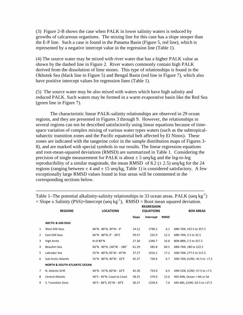
(3) Figure 2-B shows the case when PALK in lower salinity waters is reduced by growths of calcareous organisms. The mixing line for this case has a slope steeper than the E-P line. Such a case is found in the Panama Basin (Figure 5, red line), which is represented by a negative intercept value in the regression line (Table 1). (4) The source water may be mixed with river water that has a higher PALK value as shown by the dashed line in Figure 2. River waters commonly contain high PALK derived from the dissolution of lime stones. This type of relationships is found in the Okhotsk Sea (black line in Figure 5) and Bengal Basin (red line in Figure 7), which also have positive intercept values for regression lines (Table 1). (5) The source water may be also mixed with waters which have high salinity and reduced PALK. Such waters may be formed in a warm evaporative basin like the Red Sea (green line in Figure 7). The characteristic linear PALK-salinity relationships are observed in 29 ocean regions, and they are presented in Figures 3 through 9. However, the relationships in several regions can not be described satisfactorily using linear equations because of time-space variation of complex mixing of various water types waters (such as the subtropical-subarctic transition zones and the Pacific equatorial belt affected by El Ninos). These zones are indicated with the tangerine color in the sample distribution maps of Figures 3-8), and are marked with special symbols in our results. The linear regression equations and root-mean-squared deviations (RMSD) are summarized in Table 1. Considering the precision of single measurement for PALK is about ± 5 ueq/kg and the leg-to-leg reproducibility of a similar magnitude, the mean RMSD of 8.2 (± 2.5) ueq/kg for the 24 regions (ranging between ± 4 and ± 15 ueq/kg, Table 1) is considered satisfactory. A few exceptionally large RMSD values found in four areas will be commented in the corresponding sections below. ---------------------------------------------------------------------------------------------------------- Table 1–The potential alkalinity-salinity relationships in 33 ocean areas. PALK (ueq kg-1) = Slope x Salinity (PSS)+Intercept (ueq kg-1), RMSD = Root mean squared deviation.

REGIONS LOCATIONS

REGRESSION EQUATIONS BOX AREAS

Slope Intercept RMSD

ARCTIC & GIN SEAS

1 West GIN Seas 66°N - 80°N, 30°W - 0° 14.12 1796.2 6.1 68N-76N, 332.5 to 357.5

2 East GIN Seas 66°N - 80°N, 0° - 30°E 59.57 232.0 12.3 68N-76N, 2.5 to 32.5

3 High Arctic N of 80°N 27.30 1340.7 16.8 80N-88N, 2.5 to 357.5

4 Beaufort Sea 66°N - 80°N, 140°W - 180° 61.29 285.8 60.5 68N-76N, 180 to 222.5

5 Labrador Sea 55°N - 80°N, 85°W - 45°W 37.27 1016.2 17.2 56N-76N, 277.5 to 312.5

6 Sub-Arctic Atlantic 55°N - 80°N, 40°W - 10°E 45.37 730.6 6.7 56N-76N, (LON) -42.5 to +7.5

NORTH & SOUTH ATLANTIC OCEAN

7 N. Atlantic Drift 40°N - 55°N, 60°W - 10°E 45.30 733.0 6.5 44N-52N, (LON) -57.5 to +7.5

8 Central Atlantic 40°S - 40°N, Coast to Coast 58.25 270.9 12.6 40S-40N, Ocean = NA or SA

9 S. Transition Zone 40°S - 48°S, 65°W - 30°E 30.27 1259.4 7.6 44S-48S, (LON) -62.5 to +27.5

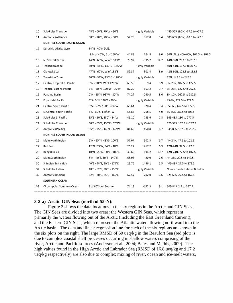
10 Sub-Polar Transition 48°S - 60°S. 70°W - 30°E Highly Variable 48S-56S, (LON) -67.5 to +27.5

11 Antarctic (Atlantic) 60°S - 70°S, 70°W - 30°E 57.78 367.8 5.4 60S-68S, (LON) -67.5 to +27.5

NORTH & SOUTH PACIFIC OCEAN

12 Kuroshio-Alaska Gyre 34°N - 40°N (All),

& N of 40°N, E of 150°W 44.88 724.8 9.0 36N (ALL), 40N-60N, 107.5 to 207.5

13 N. Central Pacific 44°N - 60°N, W of 150°W 79.92 -395.7 14.7 44N-56N, 207.5 to 237.5

14 Transition Zone 40°N - 44°N, 140°E - 145°W Highly Variable 40N-44N, 137.5 to 217.5

15 Okhotsk Sea 47°N - 60°N, W of 152°E 59.37 301.4 8.9 48N-60N, 122.5 to 152.5

16 Transition Zone 30°N - 34°N, 130°E - 120°W Highly Variable 32N, 142.5 to 242.5

17 Central Tropical N. Pacific 5°N - 30°N, W of 120°W 65.55 9.4 8.9 8N-28N, 107.5 to 122.5

18 Tropical East N. Pacific 5°N - 30°N, 120°W - 95°W 82.20 -553.2 9.7 8N-28N, 127.5 to 262.5

19 Panama Basin 0°N - 15°N, 95°W - 80°W 74.27 -290.5 8.6 8N-12N, 267.5 to 282.5

20 Equatorial Pacific 5°S - 5°N, 130°E - 80°W Highly Variable 4S-4N, 127.5 to 277.5

21 Central South Pacific 5°S - 35°S. 150°E - 84°W 66.64 -28.4 9.4 8S-36S, 142.5 to 277.5

22 E. Central South Pacific 5°S - 60°S, E of 84°W 58.88 268.5 4.0 8S-56S, 282.5 to 307.5

23 Sub-Polar S. Pacific 35°S - 50°S, 180° - 84°W 45.10 733.6 7.8 34S-48S, 180 to 277.5

24 Sub-Polar Transition 50°S - 65°S, 150°E - 70°W Highly Variable 52S-58S, 152.5 to 297.5

25 Antarctic (Pacific) 65°S - 75°S, 140°E - 65°W 81.69 450.8 6.7 64S-80S, 137.5 to 292.5

NORTH & SOUTH INDIAN OCEAN

26 Main North Indian 5°N - 25°N, 48°E - 100°E 57.07 302.3 6.7 4N-24N, 47.5 to 102.5

27 Red Sea 12°N - 27°N, 34°E - 48°E 26.27 1417.2 6.3 12N-24N, 32.5 to 47.5

28 Bengal Basin 10°N - 20°N, 80°E - 100°E 39.66 894.2 10.7 12N-24N, 77.5 to 102.5

29 Main South Indian 5°N - 40°S. 30°E - 140°E 65.03 20.0 7.6 4N-36S, 27.5 to 142.5

30 S. Indian Transition 40°S - 48°S, 30°E - 175°E 23.76 1486.1 5.5 40S-48S, 27.5 to 172.5

32 Sub-Polar Indian 48°S - 52°S, 30°E - 150°E Highly Variable None - overlap above & below

32 Antarctic (Indian) 52°S - 70°S, 25°E - 165°E 62.57 202.0 6.6 52S-68S, 22.5 to 167.5

SOUTHERN OCEAN

33 Circumpolar Southern Ocean S of 60°S, All Southern 74.13 -192.3 9.1 60S-84S, 2.5 to 357.5

----------------------------------------------------------------------------------------------------------- 3-2-a) Arctic-GIN Seas (north of 55°N): Figure 3 shows the data locations in the six regions in the Arctic and GIN Seas. The GIN Seas are divided into two areas: the Western GIN Seas, which represent primarily the waters flowing out of the Arctic (including the East Greenland Current), and the Eastern GIN Seas, which represent the Atlantic waters flowing northward into the Arctic basin. The data and linear regression line for each of the six regions are shown in the six plots on the right. The large RMSD of 60 ueq/kg in the Beaufort Sea (red plot) is due to complex coastal shelf processes occurring in shallow waters comprising of the river, Arctic and Pacific sources (Anderson et al., 2004; Bates and Mathis, 2009). The high values found in the High Arctic and Labrador Sea (RMSD of 16.8 ueq/kg and 17.2 ueq/kg respectively) are also due to complex mixing of river, ocean and ice-melt waters.

------------------------------------------------------ Figure 3 - Sample locations (upper left) and the potential alkalinity (PALK)-salinity relationships in six regions (lower left and right) in the Arctic and GIN Seas. All observations are shown in the lower left plot. The data are binned into the six regions: black = Western GIN Seas (66°N-80°N, 30°W-0°), cyan = Eastern GIN Seas (66°N-80°N, 0°-30°E), magenta = high Arctic (N of 80°N), red = Beaufort Sea (66°N-80°N, 140°W-180°), green = Labrador Sea (55°N-80°N, 85°W-45°W) and blue = Sub-Arctic Atlantic (66°N-80°N, 40°W-10°E). The same color code is used for the plots, in which linear regression lines and respective equations are shown. In the West GIN Sea plot, two lines are drawn: the cyan line is the regression line for the East GIN Sea data shown in the plot below, and the black line is the regression line for the data excluding the points, that appear to belong to the eddies from the east side.

---------------------------------------------------------- 3-2-b) Atlantic Ocean (55°N – 70°S): The PALK-salinity relationships in the North and Atlantic Ocean are shown in Figure 4. The North Atlantic drift waters (40°N-55°N) exhibit a tight linear correlation

10

(cyan plot), and have greater PALK values than the tropical and subtropical regions by 10 to 50 ueq/kg. This may be attributed to the upwelling of deep waters as well as to the mixing of the high-alkalinity low-salinity Arctic waters. The regression line for the drift coincides closely with that for the sub-Arctic Atlantic region (Figure 3) as both regions are located within the sub-polar gyre. The PALK distribution in the large expanse of the subtropical and tropical Atlantic Ocean between 40°N and 40°S may be characterized with a single linear regression line (blue plot) with a RMSD value of ± 12.6 ueq/kg. Although the subtropical South Atlantic waters tend to have somewhat lower PALK values, they are statistically indistinguishable from the northern sub-tropical waters. For this reason, the north and south sub-tropical waters are combined to yield a single regression line. In the sub-Antarctic zone (tangerine), the PALK values vary in space and time, and no systematic trend is found. The Southern Ocean waters (red plot) have about 100 ueq/kg greater PALK than the subtropical waters. This may be also accounted for by the more intense vertical mixing in the Southern Ocean. The mean RMSD for the five regions is 8.0 (± 3.2) ueq/kg.

----------------------------------------------------- Figure 4 – The North and South Atlantic Ocean is divided into five regions as shown in the map (left): cyan = North Atlantic drift region (40°N-55°N, 60°W-10°E), blue = main central Atlantic (40°N – 40°S), green = Southern transition zone (40°S-48°S, 60°W-30°E), tangerine = highly variable zone (48°S-60°S, 60°W-30°E) and red = Southern Ocean (60°S-70°S, 70°W-30°E). All data in the map areas are shown in the top left plot (black), and the data and the linear regression lines in four regions are shown in the plots (right) with the same color code as in the map. Since the data in the tangerine region are highly variable in space and time, the data and regression line in this region are not shown.

------------------------------------------------------------

3-2-c) North Pacific Ocean (60°N – the equator): The six divisions in the North Pacific Ocean are shown in Figure 5 (top left map), and the PALK-salinity relationship in the entire North Pacific is presented in the plot in the top right corner. Below them, shown are six colored plots for each of these six regions: the Okhotsk Sea (black). North Central-Bering Sea (magenta), Kuroshio-Alaska Gyre (blue), Central Tropical N. Pacific (green), Tropical East N. Pacific (cyan) and Panama Basin (red). The linear regression line and equation are shown in each of the six panels, and their colors coincide with the colors in the location map in Figure 5. The data from the tangerine areas are excluded from the analysis because of large interannual and spatial variability in the equatorial belt (i. e. ENSO) and in the northern and southern edges of the Kuroshio-North Pacific Current. The PALK-salinity relationships in the six regions of the North Pacific are described with respective linear equations (Table 1) with a mean RMSD of 10.0 (±2.3) ueq/kg. -------------------------------------------------------------- Figure 5 – Map (top left) shows the sample locations for the six areas in the North Pacific, where the PALK-salinity relationships are analyzed. The top right plot shows the entire data in the North Pacific (the equator-60°N), and the lower panels show the data and regression lines in the six regions: black = Okhotsk Sea, magenta = North Central-Bering Sea (44°N-60°N, 150°E-150°W), blue = Kuroshio-Alaska Gyre (34°N-40°N,135°E-150°W and 34°N-60°N, 150°W-125°W), green = Central Tropical N. Pacific (5°N-30°N, 120°W-120°E), cyan = Tropical East N. Pacific (5°N-30°N, 95°W-120°W) and red = Panama Basin (15N-the equator, E of 95°W). The linear regression line and equation are shown in each of the six panels, and their colors coincide with the colors in the location map. The data from the tangerine areas are excluded from the analysis because of large interannual and spatial variability.

12

----------------------------------------------------------------- 3-2-d) South Pacific Ocean (the equator-60°S): The South Pacific (including the Pacific sector of the Southern Ocean) is divided into five regions for the PALK-salinity analysis. A sub-polar region between 50°S-60°S (tangerine color) is excluded from the analysis because of large spatial and seasonal variability (Figure 6). The sub-tropical region (green) yields a linear regression line nearly consistent with the E-P line with small intercept of 28.4 (Table 1). The waters in the eastern South Pacific (blue) and in the sub-Antarctic zone (magenta) yield large positive intercept values (Table 1) due to the addition of the low-salinity high-PALK waters from the Peru upwelling zone and the Southern Ocean. The mean RMSD for the four regions is 7.0 (± 2.3) ueq/kg.

------------------------------------------------ Figure 6 – Map (top center) shows the locations for the PALK-salinity data for the four areas in the South Pacific including the Southern Ocean. The top left plot (black) shows the entire data in the South Pacific (the equator-60°N), and the other panels show the data and regression lines in the four regions: green = Central South Pacific (5°S-35°S, 84°W-150°E), blue = East Central South Pacific (5°S-60°S, E of 84°W), magenta = Sub-polar South Pacific (35°S-50°S, 84°W-180°), and red = Antarctic (Pacific Sector) (65°S-75°S, 65°W-140°E). The data from the tangerine areas are excluded from the analysis because of large interannual and spatial variability. The regression equations are listed in Table 1.

13

------------------------------------------------ 3-2-e) North Indian Ocean: (5° N – 27°N): The North Indian Ocean is divided into three regions, and the sample locations and data are shown in Figure 7. All three regions exhibit shallower slopes than the E-P line with positive intercepts (Table 1). The positive intercept found for the Main North Indian region may be attributed to CaCO3 production in high salinity waters as well as to the input of the high-PALK Indus River waters. The large positive intercept observed for the Red Sea is due to intense evaporation (high salinity) coupled with CaCO3 production. The Bengal Basin trend is primarily due to the influx of the high PALK Ganges-

14

Brahmaputra river waters. The regression equations are listed in Table 1, and the mean RMSD for these three regions is 7.9 (±2.3) ueq/kg.

------------------------------------------------------ Figure 7 –Map (top center) shows the locations for the PALK-salinity data for the three areas in the North Indian Ocean (5°N – 27°N) including the Red Sea. The top left plot (black) shows the entire data in the region, and the other panels show the data and regression lines in the three regions: blue = Main North Indian Ocean (25°N (10°N)-5°N, 48°E-100°E), green = Red Sea (12°N-27°N, 34°E-48°E), and red = Bengal Basin (10°N-20°N, 80°E-100°E). Note that the salinity axis is expanded to 41.0 because of the high salinity waters of the Red Sea. The regression equations are listed in Table 1.

------------------------------------------------------

3-2-f) South Indian Ocean: (5° N – 70°S): The South Indian Ocean is divided into three regions. The PALK-salinity trend (blue plot) for the Main South Indian Ocean region (5°N-40°S), which covers the sub-tropical and tropical oceans, has a slope nearly equal to the E-P slope, but with a small positive intercept reflecting the CaCO3 production. The Southern Ocean water has about

15

100 ueq/kg greater PALK than the sub-tropical and tropical waters, due to the upwelling of the deep waters in the Southern Ocean. The flat trend (green plot) for the South Indian Transition zone represents a mixing line between the subtropical and Southern Ocean waters. The mean RMSD for the three regions is 6.5 (±1.1) ueq/kg.

--------------------------------------------------------- Figure 8 – Figure 8 - Map (top center) shows the locations for the PALK-salinity data for the three areas in the South Indian Ocean (5°N – 70°S). The top left plot (black) shows the entire data in the region, and the other panels show the data and regression lines in the three regions: blue = Main South Indian Ocean (5°N-40°S, 30°E-140°E ), green = S. Indian Transition (40°S-48°S, 30°E-150°E), and red = Antarctic (Indian Sector) (52°S-70°S, 25°E-165°E). The data from the tangerine areas (48°S-52°S) are excluded from the analysis because of large interannual and spatial variability. The regression equations are listed in Table 1.

---------------------------------------------------------

16

3-2-g) Southern Ocean: (south of 60°S): The PALK-salinity relationships in each of the Atlantic, Pacific and Indian sectors of the Southern Ocean have been analyzed separately in order to illustrate the differences between the subtropical waters and the polar waters. However, as shown in Table 1, the trends in each of these sectors are found to vary widely. This may be attributed to a narrow salinity range (33.0 - 34.8) as well as to uneven seasonal and spatial distribution of samples. Variability of PALK may be caused by regional differences in lateral, vertical mixing and processes associated with sea and continental ice, and measurements are made more often during non-winter months. Nevertheless, the PALK data in the circumpolar surface waters are assembled (Figure 9) and analyzed to show that the data may be represented by a single linear regression line with a RMSD of 9.1 ueq/kg (Table 1). The negative intercept (-192.2 ueq/kg) may be attributed to greater upwelling of deep waters in higher salinity areas. This relationship is used for the calculation of the distribution of pH and others, rather than the regression lines for each of the Atlantic, Indian and Pacific sectors of the Southern Ocean.

--------------------------------------------------------- Figure 9 – Sample locations (left) and the PALK-salinity plot (right) for the Southern Ocean (south of 60°S). The linear regression line and equation are indicated in the data plot to the right.

----------------------------------------------------------- 3-3 Global Distribution of Total Alkalinity:

To obtain pH, degree of saturation for CaCO3, we need the total alkalinity (TA). First, the global distribution of the potential alkalinity (PALK) is obtained using its relationship with salinity presented above for various ocean regions (Table 1) and the climatological salinity for the global oceans (NCEP Reanalysis data, 2001; Atlas of Surface Marine Data, 1994). Then, the total alkalinity (TA) is obtained by subtracting the climatological mean concentration of nitrate (Conkright et al., 1994; Levitus et al., 1994)

17

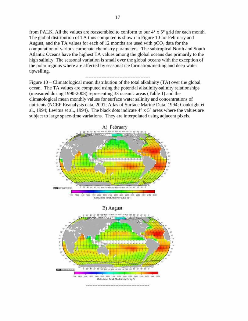
from PALK. All the values are reassembled to conform to our 4° x 5° grid for each month. The global distribution of TA thus computed is shown in Figure 10 for February and August, and the TA values for each of 12 months are used with pCO2 data for the computation of various carbonate chemistry parameters. The subtropical North and South Atlantic Oceans have the highest TA values among the global oceans due primarily to the high salinity. The seasonal variation is small over the global oceans with the exception of the polar regions where are affected by seasonal ice formation/melting and deep water upwelling.

---------------------------------------- Figure 10 – Climatological mean distribution of the total alkalinity (TA) over the global ocean. The TA values are computed using the potential alkalinity-salinity relationships (measured during 1990-2008) representing 33 oceanic areas (Table 1) and the climatological mean monthly values for surface water salinity and concentrations of nutrients (NCEP Reanalysis data, 2001; Atlas of Surface Marine Data, 1994; Conkright et al., 1994; Levitus et al., 1994). The black dots indicate 4° x 5° areas where the values are subject to large space-time variations. They are interpolated using adjacent pixels. A) February

B) August

---------------------------------------

18

3-4. Climatological Distribution of Surface Water pCO2:

The second carbon chemistry parameter needed for computing pH and associate properties, we select pCO2 in surface ocean water. Its climatological monthly mean values over the global ocean are computed for a 4° x 5° grid for the reference year 2005 (Figure 11). This is an updated version of Takahashi et al. (2009) for the reference year 2000 representing non-El Nino years, and is based on about sing 6 million pCO2 data observed in 1957-2011 (Takahashi et al., 2012), which include 2.5 million new data obtained since 2000. The updated 4° x 5° gridded data for each of 12 months in 2005 are available at our web site, http://www.ldeo.columbia.edu/res/pi/CO2, and the February and August values are shown in Figure 10. Large seasonal changes observed in the subtropical gyre areas are attributed primarily to the seasonal temperature changes; the changes in the polar areas are due to upwelling of deep waters in winter and intense photosynthesis during summer. Compared to the previous distribution for 2000, the 2005 pCO2 values are 10 ± 3 uatm greater on the global average.

------------------------------------------ Figure 11 – Climatological mean distribution of the surface water pCO2 over the global oceans in the reference year 2005: (A) February, 2005 and (B) August, 2005. These maps have been up-dated to the reference year 2005 using a total of about 6 million pCO2 measurements (Takahashi et al., 2012) which include about 2.5 million new data acquired since 2000. The monthly mean pCO2 values for each of 12 months are used for calculating the pH, TCO2 and other parameters, only February and August distributions are shown here. The heavy pink curves indicate the mean position of the equator-ward extent of ice fields. A) February, 2005

19

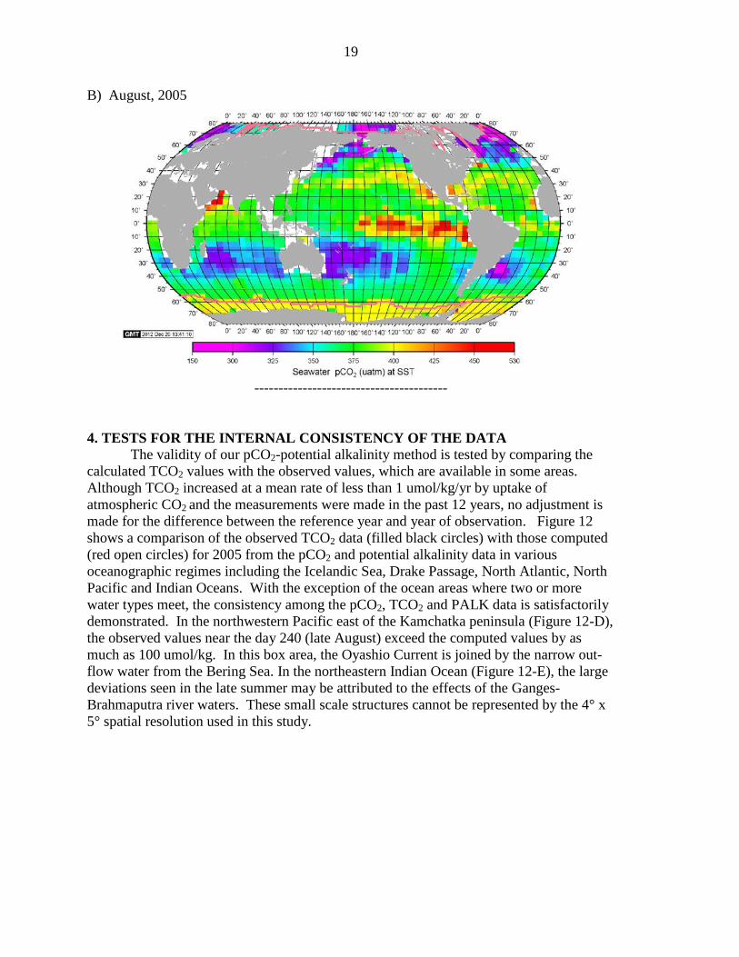
B) August, 2005

----------------------------------------

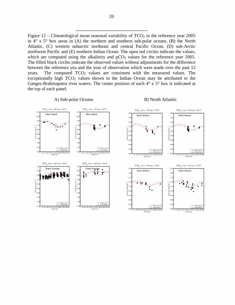
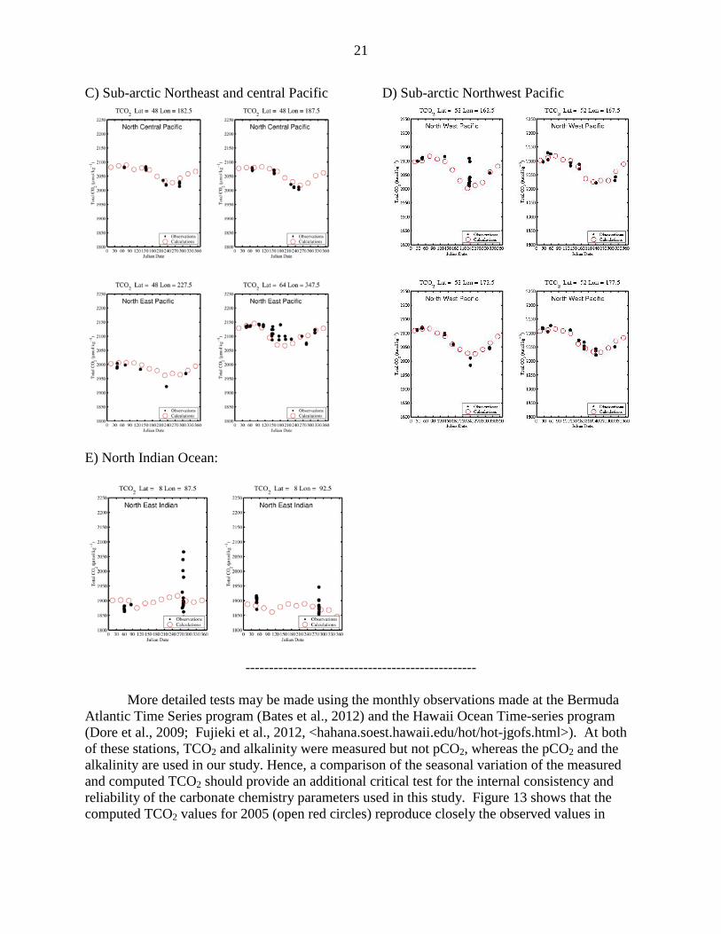
4. TESTS FOR THE INTERNAL CONSISTENCY OF THE DATA The validity of our pCO2-potential alkalinity method is tested by comparing the calculated TCO2 values with the observed values, which are available in some areas. Although TCO2 increased at a mean rate of less than 1 umol/kg/yr by uptake of atmospheric CO2 and the measurements were made in the past 12 years, no adjustment is made for the difference between the reference year and year of observation. Figure 12 shows a comparison of the observed TCO2 data (filled black circles) with those computed (red open circles) for 2005 from the pCO2 and potential alkalinity data in various oceanographic regimes including the Icelandic Sea, Drake Passage, North Atlantic, North Pacific and Indian Oceans. With the exception of the ocean areas where two or more water types meet, the consistency among the pCO2, TCO2 and PALK data is satisfactorily demonstrated. In the northwestern Pacific east of the Kamchatka peninsula (Figure 12-D), the observed values near the day 240 (late August) exceed the computed values by as much as 100 umol/kg. In this box area, the Oyashio Current is joined by the narrow out-flow water from the Bering Sea. In the northeastern Indian Ocean (Figure 12-E), the large deviations seen in the late summer may be attributed to the effects of the Ganges-Brahmaputra river waters. These small scale structures cannot be represented by the 4° x 5° spatial resolution used in this study.

20

----------------------------------------------- Figure 12 – Climatological mean seasonal variability of TCO2 in the reference year 2005 in 4° x 5° box areas in (A) the northern and southern sub-polar oceans, (B) the North Atlantic, (C) western subarctic northeast and central Pacific Ocean, (D) sub-Arctic northwest Pacific and (E) northern Indian Ocean. The open red circles indicate the values, which are computed using the alkalinity and pCO2 values for the reference year 2005. The filled black circles indicate the observed values without adjustments for the difference between the reference yea and the year of observation which were made over the past 12 years. The computed TCO2 values are consistent with the measured values. The exceptionally high TCO2 values shown in the Indian Ocean may be attributed to the Ganges-Brahmaputra river waters. The center position of each 4° x 5° box is indicated at the top of each panel. A) Sub-polar Oceans

B) North Atlantic

21

C) Sub-arctic Northeast and central Pacific D) Sub-arctic Northwest Pacific

E) North Indian Ocean:

------------------------------------------------- More detailed tests may be made using the monthly observations made at the Bermuda Atlantic Time Series program (Bates et al., 2012) and the Hawaii Ocean Time-series program (Dore et al., 2009; Fujieki et al., 2012, <hahana.soest.hawaii.edu/hot/hot-jgofs.html>). At both of these stations, TCO2 and alkalinity were measured but not pCO2, whereas the pCO2 and the alkalinity are used in our study. Hence, a comparison of the seasonal variation of the measured and computed TCO2 should provide an additional critical test for the internal consistency and reliability of the carbonate chemistry parameters used in this study. Figure 13 shows that the computed TCO2 values for 2005 (open red circles) reproduce closely the observed values in

22

2005-2006 (filled black circles), capturing the seasonal variability. This gives further credence to the pCO2-TA method used in this study.

--------------------------------------------------- Figure 13 – Comparison of the observed and calculated TCO2 at the BATS and HOT time-series stations. The 2005-2006 observations (from the BATS database) are shown with filled black circles. The calculated values for 2005 in the 4° x 5° boxes which include these stations are shown with open red circles. The BATS station is located in the box centered at 32°N and 62.5°W. The HOT station is located near the border of two 4° x 5° boxes, and the data for the box centered at 20°N and 157.5°W are shown. The computed TCO2 values are consistent with the observed, capturing the seasonal variability. (A) BATS (31.7°N, 64.2°W)

(B) HOT (22.75°N, 158.0°W)

-------------------------------------------------- 5. RESULTS 5-1) Climatological Mean Distribution:

The climatological mean distribution maps for pH, degree of saturation for aragonite and calcite in surface waters of the global oceans for the reference year 2005 are presented in this section. These are calculated using the following information; a) climatological mean monthly pCO2 in surface water in 4° x 5° box areas for the reference year 2005 (see Section 5); b) the potential alkalinity-salinity relationships representing 29 oceanic areas (based on the measurements made 1990-2008, Section 3.2); c) climatological mean monthly values for surface water temperature, salinity and concentrations of nutrients (NCEP Reanalysis data, 2001; Atlas of Surface Marine Data, 1994; Conkright et al., 1994; Levitus et al., 1994); and d) the inorganic carbonate chemistry model described in Section 2. The degree of saturation for aragonite and calcite is expressed in Ω = [Ca++]sw x [CO3

=]sw / Ksp’, where Ksp’ is the solubility products

23

CaCO3 formulated by Mucci (1983) for aragonite and calcite. The calcium concentration in seawater is estimated by [Ca++]sw (mol/kg) = 0.01012 x (salinity)/35. Supersaturation is indicated by Ω > 1.0, and undersaturation by Ω < 1.0.

As shown in the global maps below for all the carbon chemistry properties, the Indian

Ocean has different properties from the Pacific and Atlantic Oceans. The differences are especially pronounced in the northern Indian Ocean. In the Indian Ocean TA is lower (Figure 10) and pCO2 is higher (Figure 11) than the Atlantic and Pacific. The computed properties including pH (Figure 14), Ω for aragonite and calcite (Figures 15 and 16) and TCO2 (Figure 17) are all lower in the Indian Ocean than the Atlantic and Pacific reflecting these differences. The causes for these differences are not understood because of the complexity which is unique to the Indian Ocean, which extends only to about 30°N. In the northwestern Indian Ocean, the Arabian Sea receives a number of different waters including the intense summer upwelling of deep waters, high salinity, warm outflow waters from the Red Sea and Persian Gulf and the Indus River waters. The northeastern Indian Ocean receives from the east the low salinity Indonesian outflow and from the north the Ganges- Brahmaputra river waters. The Arabian Sea water is generally warmer and saltier than the Bengal Gulf. Furthermore, the surface water circulation is reorganized extensively in response to the monsoons. Therefore, further observational and model studies are needed for improved understanding of the uniqueness of the Indian Ocean.

5-1-a) pH:

The distribution of pH (total H+ scale, at in situ temperatures) in surface waters is presented in Fig.14 for February and August. The values for these and the other months are listed in our web site. The pH values range from 7.9 to 8.2 in 2005. Lower (more acidic) values are found in the upwelling regions in the Panama Basin (in the equatorial Pacific), Arabian and Bering Seas; and higher values are found in the sub-polar and polar waters during the spring-summer months of intense photosynthetic production. The vast areas of subtropical oceans have seasonally varying pH values ranging from 8.05 during warmer months to 8.15 during colder months. In the high-nutrient subpolar and polar waters, pH is lower during winter due to the upwelling of more acidic deep waters, and it increases during summer due to intense photosynthetic utilization of CO2. Accordingly, the seasonal pH change in subpolar oceans is six months out of phase with that in the adjacent subtropical ocean.

Fig. 14 shows that northern Indian Ocean has lower pH (more blue) than the subtropical North Pacific and North Atlantic, especially during the northern winter months. This has been discussed at the beginning of Section 5.

----------------------------------------------------------- Figure 14 –The climatological mean distribution of pH (total H+ scale at in situ temperatures) in the global ocean surface water in (A) February and (B) August in the reference year 2005. The pink curves indicate the position of the mean equator-ward front of seasonal ice fields. The “+” symbol indicates the box areas affected by the El Nino events, and no value is given because of large space-time variability. The boxes with black dots are in a transition zone between oceanographic regimes (such as subtropical to subpolar regimes), where the pH values are highly variable.

24

(A) Calculated pH for February, 2005

(B) Calculated pH for August, 2005

-------------------------------------------------------------

5-1-b) Degree of Saturation for Aragonite and Calcite:

Surface waters of the global oceans are generally supersaturated with respect to aragonite and calcite. As shown in Fig. 15, the warm tropical and subtropical waters are supersaturated with respect to aragonite by as much as 4 times (or 400% supersaturation), whereas the cold subpolar and polar waters are supersaturated only by 1.2 times (or 20% supersaturation) or less. While the seasonal variation is small in the subtropical waters, the subpolar waters exhibit larger seasonal changes ranging from Ω of 1.5 in winter months and Ω of 2.0 in summer months. In a recent study in the western and central Arctic, aragonite undersaturation (Ω as low as 0.8) has been reported (Robbins et al., submitted).

25

Figure 15 shows that, while the Ω values for the subtropical Pacific and Atlantic are similar, those in the subtropical Indian Ocean are generally lower (i. e. less saturated, more yellowish). This reflects the lower pH values (Figure 13), and the causes for the uniqueness of the Indian Ocean have been discussed at the beginning of Section 5.

------------------------------------------------------- Figure 15 –The climatological mean distribution of aragonite saturation level (Ω) in the global ocean surface water in (A) February and (B) August in the reference year 2005. The pink curves indicate the position of the mean equator-ward front of seasonal ice fields. The “+” symbol indicates the box areas affected by the El Nino events, and no value is given because of large space-time variability. The boxes with black dots are in a transition zone between oceanographic regimes (such as subtropical to subpolar regimes), where the Ω values are highly variable. Note that the Arctic Ocean is slightly below the saturation (Ω < 1.0), whereas the Southern Ocean is somewhat above the saturation.

A) February, 2005

B) August, 2005

-------------------------------------------------------

26

The distribution maps of calcite saturation for February and August, 2005, are shown in Figure 16. The Ω values range between 1.8 in the polar regions to 6.3 in subtropical waters. The observed pattern of distribution is similar to that for aragonite, the north and south Indian Oceans are shown to have lower degree of saturation than the Pacific and Atlantic. The causes for this feature have been discussed at the beginning of Section 5.

------------------------------------------------------- Figure 16 – The climatological mean distribution of calcite saturation level (Ω) in the global ocean surface water in (A) February and (B) August in the reference year 2005. The pink curves indicate the position of the mean equator-ward front of seasonal ice fields. The “+” symbol indicates the box areas affected by the El Nino events, and no value is given because of large space-time variability. The boxes with black dots are in a transition zone between oceanographic regimes (such as subtropical to subpolar regimes), where Ω values are highly variable.

A) February, 2005

B) August, 2005

--------------------------------------------------------

27

5-1-c) TCO2 in surface water: The distribution maps of TCO2 for February and August, 2005, are shown in Figure 17. The TCO2 values range between 2225 umol/kg in the polar regions to 1875 umol/kg in subtropical waters. They are higher due to winter reflecting deep water upwelling, and are lower during summer due to biological CO2 utilization. The amplitude for seasonal change is generally about 75 umol/kg for the subpolar waters, while that for subtropical waters is less and correlates with the seasonal SST amplitude. The north and south Indian Oceans are shown to have lower TCO2 values than the Pacific and Atlantic. The causes for this feature have been discussed at the beginning of Section 5.

--------------------------------------------------- Figure 17 –The climatological mean distribution of TCO2 in the global ocean surface water in (A) February and (B) August in the reference year 2005. The TCO2 values are computed using the total alkalinity (TA) and pCO2. The pink curves indicate the position of the mean equator-ward front of seasonal ice fields. The “+” symbol indicates the box areas affected by the El Nino events, and no value is given because of large space-time variability. The boxes with black dots are in a transition zone between oceanographic regimes (such as subtropical to subpolar regimes), where ΤCΟ2 values are highly variable.

A) February, 2005

B) August, 2005

--------------------------------------------------

28

5-2) Time Trend: The decadal mean trend for observed and calculated parameters is presented for the BATS and HOT time-series stations in Figure 18 and the Drake Passage sites in Figure 19. At the BATS and HOT stations, TA and TCO2 were measured, and the pCO2 and pH values are computed. On the other hand, at the Drake Passage sites, TCO2 and pCO2 were measured, and pH and TA are computed. The computations were made using the equilibrium carbonate chemistry model described in Section 2 of this paper, so that these values are consistent with the global values presented in this paper. Figure 18 shows significant differences in the seasonal variability between BATS in the northwestern Atlantic and HOT in the central north Pacific subtropical gyre. The seasonal amplitude for SST at BATS is about 10°C and it is about 4°C at HOT, although the annual mean SST is about 24°C at both sites. The seasonal amplitude for pCO2, TCO2 and pH at BATS are respectively 100 uatm, 50 umol/kg and 0.1 respectively, whereas those at HOT are 30 uatm, 20 umol/kg and 0.04 respectively and are about 1/3 of the BATS values. These differences appear to reflect the differences in the mixed layer depth and the vertical mixing rate across the base of the mixed layer. In spite of these differences, the decadal mean rate for pCO2 increase at these stations is similar at 1.8 uatm/yr at BATS and 1.9 uatm/yr at HOT, and the surface ocean waters appear to be tracking the atmospheric CO2 increase. The pH changes are also similar at these stations, both yielding an acidification rate of 0.0018 pH/yr.

------------------------------------------------- Figure 18 – Time trends observed at the BATS and HOT stations. The temperature, salinity, alkalinity and TCO2 data are provided by the websites for the Bermuda Time-Series program (Bates et al., 2012) and the Hawaii Ocean Time-series program (Fujieki et al., 2012,<hahana.soest.hawaii.edu/hot/hot-jgofs.html>). The pCO2 and pH values are computed using the equilibrium carbonate chemistry model described in Section 2 of this paper.

---------------------------------------------------

29

The 2002-2012 decadal time-series data obtained by the LDEO staff across the Drake Passage, Southern Ocean are shown in Figure 19. The left column represents the Antarctic Circumpolar Water, north of the Polar Front between 220 km and 350 km from the southern tip of South America, and the right column represents the Polar Water south of the Polar Front and north of the Continental Water (between 580 km and 720 km from South America). In the waters north of the Polar Front, pCO2 increases at a rate of 1.9 uatm/yr, which is consistent with the rates observed at BATS and HOT as well as the rate of atmospheric CO2 increase rate. The rate of pH decrease is found to be 0.002 pH/yr, which is also consistent with those found in the subtropical waters at BATS and HOT. It, therefore, appears that the surface waters of nearly entire global ocean are tracking the atmospheric CO2 increase rate of 1.9 ppm/yr, and are being acidified at a mean rate of -0.002 pH/yr. In contrast to the Circumpolar Water, the Continental Water shows little change in pCO2 and pH. Its behavior appears to be decoupled from the rest of the global oceans and governed by the regional processes associated with the Antarctic continent.

--------------------------------------------------- Figure 19 - The monthly mean values for SST, pH, pCO2,TCO2,TALK, PO4 and Ω aragonite in the surface water in the Drake Passage, Southern Ocean for a zone north of the Polar Front (220 – 350 km from the southern tip of South America) and a zone south of it (580-720 km from the southern tip). The decadal mean rate of change is based upon the linear regression (heavy line), and is shown in the box. The uncertainty is computed using ± σ2/(ΣXi2 – N (mean Xi)2, where σ2 is Σ(Yi – aXi – b)2/(N-2), N is the number of years, and Xi is decimal year.

---------------------------------------------------

30

6. SMMARY AND CONCLUSION 1) A database for the alkalinity, pCO2 and the concentrations of total CO2 and nutrients in the surface ocean waters (depths < 50 meters) over the global oceans is assembled by building upon the data synthesis of the GLODAP database (Key et al., 2004) supplemented with the TCO2-TA pairs from the CARINA program (Tanhua et al., 2009; Key et al., 2010) and pCO2 and TCO2 data from the LDEO database. Based on this database, the distributions of pH, degree of saturation for aragonite and calcite and TCO2 over the global ocean are obtained. 2) The global distribution of surface water TA is obtained using the potential alkalinity-salinity relationships (linear regressions) in 32 of ocean regions (excluding the equatorial Pacific El Nino zone). Using the mean monthly pCO2 data adjusted to a reference year 2005 and the alkalinity estimated using the potential alkalinity-salinity relationships, the mean monthly distributions of pH and aragonite saturation in surface ocean waters are obtained for the year 2005. 3) The mutual consistency between TA-TCO2-pCO2 values used for the computation of pH and degree of saturation of CaCO3 is tested and validated using the available observations including the time-series data obtained at BATS and HOT programs. This verifies the uniformity of the pH and other parameters computed for the global oceans. 4) The pH in the global ocean surface waters ranges from 7.9 to 8.2 in the year 2005. Lower values are located in the upwelling regions in the equatorial Pacific and in the Arabian and Bering Seas; and higher values are found in the subpolar and polar waters during the spring-summer months of intense photosynthetic production. The vast areas of subtropical oceans have seasonally varying pH values ranging from 8.05 during warmer months to 8.15 during colder months. The warm tropical and subtropical waters are supersaturated by a factor of as much as 4.2 with respect to aragonite and 6.3 for calcite, whereas the cold subpolar and polar waters are less supersaturated only by a factor of 1.2 for aragonite and 2 for calcite because of the lower pH values resulting from greater TCO2 concentration. In the western Arctic Ocean, aragonite undersaturation is observed. 5) Decadal time-series data at the Bermuda (BATS), Hawaii (HOT) and Drake Passage (Antarctic Circumpolar Water) show that pH has been declining at a mean rate of about -0.002 pH per year, and that the pCO2 has been increasing at a rate of 1.9 uatm/yr, which is consistent with the recent atmospheric CO2 increase rate of 1.9 ppm/yr. This suggests that the global oceans are being acidified uniformly at a mean rate of about -0.002 pH/yr, responding to the increase in the atmospheric CO2. 7. REFERENCES CITED Anderson, L. G., Jutterstrom, S., Kaltin, S., Jones, P. E. and Bjork, G. (2004). Variability in river runoff distribution in the Eurasian Basin of the Arctic Ocean. Journ. Geophys. Res., 109, CO1016, doic:10.1029/2003JC001773, 204.

31

Atlas of Surface Marine Data (1994). CD-ROM NODC-56, Ocean Climate Laboratory, NOAA, Washington, D. C. Balch, W. M., H. R. Gordon, B. C. Bowler, D. T. Drapeau, and E. S. Booth (2005), Calcium carbonate budgets in the surface global ocean based on MODIS data, J. Geophys. Res., 110, C07001, doi:10.1029/2004JC002560. Bates, N. R., Michaels, A. F., and Knap, A. H.. (1996). Seasonal and interannual variability of oceanic carbon dioxide species at the US JGOFS Bermuda Atlantic Time-series Study (BATS) site, Deep-Sea Res. II, 43, 347–383, doi:10.1016/0967-0645(95)00093-3,Corrigendum: 43, 1435–1435, 1996. Bates, N. R. and Mathis, J. T. (2009). The Arctic Ocean marine carbon cycle: evaluation of air-sea CO2 exchanges, ocean acidification impacts and potential feedbacks. Biogeosciences, 6, 2433-2459. www.biogeosciences.net/6/2433/2009/. Bates, N. R., M. H. P. Best, K. Neely, R. Garley, A. G. Dickson, and R. J. Johnson (2012). Detecting anthropogenic carbon dioxide uptake and ocean acidification in the North Atlantic Ocean. Biogeosciences, 9, 2509–2522, www.biogeosciences.net/9/2509/2012/doi:10.5194/bg-9-2509-2012. Brewer, P. G. and Goldman, J. C. (1976). Alkalinity changes generated by phytoplankton growth. Lim. and Oceanogr., 21, 108-117. Conkright, M., Levitus, S.and Boyer, T., (1994). World Ocean Atlas, 1994: Volume 1, Nutrients. NOAA Atlas NESDIS 1, National Oceanic and Atmospheric Administration, Washington, D. C., 150 pp. Dickson, A. G. and J. P. Riley (1979-a). The estimation of acid dissociation constants in seawater media from potentiometric titrations with strong base. I. The ionic product of water (Kw). Marine Chem., 7, 89-99. Dickson, A. G. and J. P. Riley (1979-b). The estimation of acid dissociation constants in seawater media from potentiometric titrations with strong base. II. The dissociation of phosphoric acid. Marine Chem., 7, 101-109. Dickson, A. G. (1990). Thermodynamics of the dissociation of boric acid in synthetic seawater from 273.15 to 318.15K. Deep-Sea Res., 37, 755-766. Dickson, A. G. (2001). Reference materials for oceanic CO2 measurements. Oceanography, 14, 21-22.

Doney, S. C, Fabry, V. J, Feely, R. A., and Kleypas, J. A. (2009), Ocean acidification: the other CO2 problem. Ann. Rev. Mar. Sci., 1, 169-192

32

Dore, J. E., Lukas, R., Sadler, D. W., Church, M. J. and Karl, D. M. (2009). Physical and biogeochemical modulation of ocean acidification in the central North Pacific. PNAS, 106, 12235-12240. doi:10.1073.pnas.0906044106. Feely, R. A., Sabine, C. L., Lee, K., Berelson, W., Kleypas, J., Fabry, V. J. and Millero, F. J. (2004). Impact of anthropogenic CO2 on the CaCO3 system in the oceans. Science, 305, 362-366. Feely, R.A., Doney, S. C. and Cooley, S. R. (2009). Ocean acidification: Present conditions and future changes in high-CO2 world. Oceanography, 22, 36-47. Key, R. M., Kozyr, A., Sabine, C. L., Lee, K., Wanninkhof, R., Bullister, J. L., Feely, R. A., Millero, F. J., Mordy, C. and Peng, T.H. (2004). A global ocean carbon climatology: Results from Global Data Analysis Project (GLODAP). Glob. Biogeochem. Cycles, 18 (4): doi. GB4031 DEC 29 2004. Key, R. M., Tanhua, T., Olsen, A., Hoppema, M., Jutterstrom,S., Schirnick, C., van Heuven, S., Kozyr, A., Lin, X., Wallace, D. W. and Mintrop, L. (2010). The CARINA data synthesis project: introduction and overview. Earth Syst. Sci. Data, 2, 105-121. www.earth-syst-sci-data.net/2/105/2010. Lee, K., Tong, L. T., Millero, F. J., Sabine, C. L., Dickson, A. G., Goyet, C., Park, G-H., Wanninkhof, R., Feely, R. A. and Key, R. M. (2006). Global relationships of total alkalinity with salinty and temperature in surface watrs of the world’s oceans. Geophys. Res. Let. 33, L19605, doi:10.1029/2006GL27207. Levitus, S., Burgett, R. and Boyer, T. (1994). World Ocean Atlas, 1994: Volume 3, Salinity. NOAA Atlas NESDIS 3, National Oceanic and Atmospheric Administration, Washington, D. C., 99 pp. Lueker, T. J., Dickson, A. G. and Keeling, C. D. (2000). Ocean pCO2 calculated from dissolved inorganic carbon, alkalinity and equations K1 and K2: validation based on laboratory measurements of CO2 in gas and seawater at equilibrium. Marine Chem., 70, 105-119. NCEP Reanalysis data (2001). NCEP/NCAR Reanalysis Monthly Means and Other Derived Variables, provided by the NOAA-CIRES Climate Diagnostics Center, Boulder, CO. http://www.cdc.noaa.gov/cdc/data/ncep.reanalysis.derived.html Orr, J. C. and 26 coauthors, (2005). Anthropogenic ocean acidification over the twenty-first century and its impact on calcifying organisms. Nature, 437, 681-686. doi: 10.1038/nature04095. Santana-Casiano, J. M., M. Gonza´lez-Da´vila, M.-J. Rueda, O. Llina´s, and E.-F. Gonza´lez-Da´vila (2007), The interannual variability of oceanic CO2 parameters in the northeast Atlantic subtropical gyre at the ESTOC site, Global Biogeochem. Cycles, 21,

33

GB1015, doi:10.1029/2006GB002788. Sjorberg, S., N. Nordin and N. Ingri (1981). Equilibrium and structural studies of silicon(IV) and aluminium(III) in aqueous solution. II. Formation constants for the monosilicate ions SiO(OH)3- and SiO2(OH)2

2-. A precision study at 25 oC in a simplified seawater medium. Marine Chem., 19, 521-532. Takahashi, T., et al. (2009). Climatological mean and decadal changes in surface ocean pCO2, and net sea-air CO2 flux over the global oceans. Deep-Sea Res. II, 554-577. doi: 10.1016/j.dsr2.2008.12.009. Takahashi, T., S.C. Sutherland, and A. Kozyr. (2012). Global Ocean Surface Water Partial Pressure of CO2 Database: Measurements Performed During 1957–2011 (Version 2011). ORNL/CDIAC-160, NDP-088(V2011). Carbon Dioxide Information Analysis Center, Oak Ridge National Laboratory, U.S. Department of Energy, Oak Ridge, Tennessee, doi: 10.3334/CDIAC/OTG.NDP088(V2011). Tanhua, T. et al. (2009). CARINA Data Synthesis Project. ORNL/CDIAC-157, NDP-091, Oak Ridge National Laboratory, U. S. Department of Energy, pp. 11. Weiss, R. F. (1974). Carbon dioxide in water and seawater: The solubility of a non-ideal gas, Marine Chem., 2, 203-215.