Institute of General Mechanics RWTH Aachen University

M. Chen, A. Hachemi, D. Weichert

3nd International Workshop on Direct Methods, October 20-21, 2011, Athens

Progress in plastic design

of composites

BACKGROUND

*http://www.boeing.com

Composites: Increasing application Multi-scale approach (Meso-/Micromechanics) Local and global design

Direct Methods: Unknown loading history Economic design ( permission of plastic deformation)

Composite Materials at Boeing 787 *

CONTENTS

Direct methods applied to composites • Elements of homogenization theory • Finite element discretization

Kinematic hardening • Unlimited kinematic hardening • Limited kinematic hardening

Failure criterion of composites • Plane stress • Plane strain ( 3D general stress state)

Numerical illustration • Effective material properties • Yield criterition fitting • Kiematic hardening

Conclusions

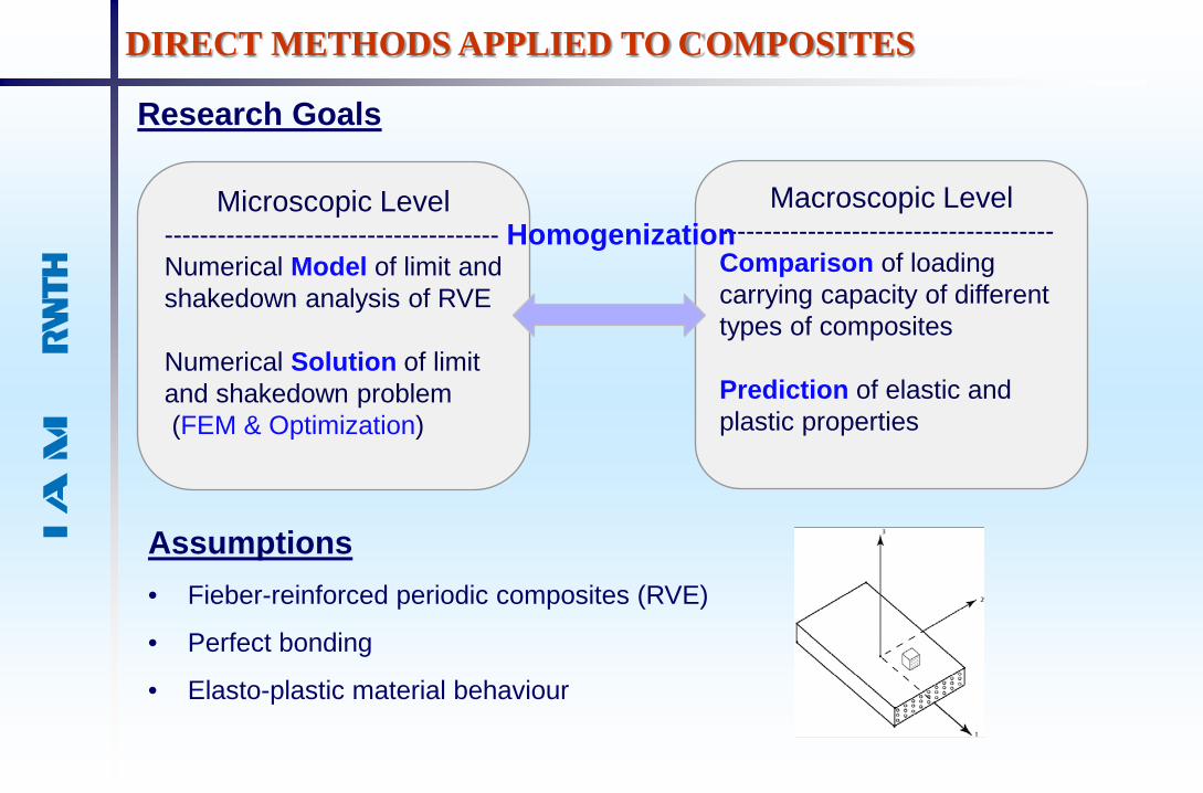
Research Goals

Microscopic Level -------------------------------------- Numerical Model of limit and shakedown analysis of RVE Numerical Solution of limit and shakedown problem (FEM & Optimization)

Macroscopic Level -------------------------------------- Comparison of loading carrying capacity of different types of composites Prediction of elastic and plastic properties

Homogenization

DIRECT METHODS APPLIED TO COMPOSITES

Assumptions • Fieber-reinforced periodic composites (RVE)

• Perfect bonding

• Elasto-plastic material behaviour

ELEMENTS OF HOMOGENIZATION THEORY

* Suquet, P.: Doctor Thesis, Pierre & Marie Curie, (1982)

Concept of representative volume element (RVE)

Heterogeneous Material RVE Homogenized Material

Localisation Globalisation

𝜉𝜉 = 𝑥𝑥 𝜃𝜃⁄ , θ: a small parameter

Average field quantities*

𝜮𝜮(𝑥𝑥) =1𝑉𝑉 � 𝝈𝝈(𝜉𝜉) d𝑉𝑉 = ⟨𝝈𝝈(𝜉𝜉)⟩𝑉𝑉

𝑬𝑬(𝑥𝑥) =1𝑉𝑉 � 𝜺𝜺(𝜉𝜉) d𝑉𝑉 = ⟨𝜺𝜺(𝜉𝜉)⟩𝑉𝑉

DIRECT METHODS APPLIED TO COMPOSITES

* D.Weichert, A.Hachemi and F.Schwabe. Mech. Res. Comm. 26(3), 309-318 (1999)

** H.Magoariec, S.Bourgeois and O.Débordes. Int. J. Plasticity. 20, 1655-1675 (2004)

𝜮𝜮 =1𝑉𝑉�(𝛼𝛼𝝈𝝈𝒆𝒆 + 𝝆𝝆�) d𝑉𝑉𝑉𝑉

=1𝑉𝑉� 𝛼𝛼𝝈𝝈𝒆𝒆 d𝑉𝑉𝑉𝑉

+1𝑉𝑉� 𝝆𝝆� d𝑉𝑉𝑉𝑉

𝑤𝑤𝑤𝑤𝑤𝑤ℎ 1𝑉𝑉� 𝝆𝝆� d𝑉𝑉𝑉𝑉

= 0

Static direct methods for periodic composites*

𝓟𝓟𝐬𝐬𝐬𝐬𝐬𝐬𝐬𝐬𝐬𝐬𝐬𝐬

⎩⎪⎨

⎪⎧ div 𝝈𝝈𝐸𝐸 = 0 in 𝑉𝑉

𝝈𝝈𝐸𝐸 = 𝒅𝒅: (𝑬𝑬 + 𝜺𝜺𝐩𝐩𝐩𝐩𝐬𝐬) in 𝑉𝑉 𝝈𝝈𝐸𝐸 ∙ 𝒏𝒏 anti − periodic on 𝜕𝜕𝑉𝑉 𝒖𝒖per periodic on 𝜕𝜕𝑉𝑉 ⟨𝜺𝜺⟩ = 𝜠𝜠

𝓟𝓟𝐬𝐬𝐬𝐬𝐬𝐬𝐬𝐬𝐬𝐬𝐬𝐬𝐬𝐬𝐩𝐩𝐬𝐬 �div 𝝆𝝆� = 0 in 𝑉𝑉

𝝆𝝆� ∙ 𝒏𝒏 anti − periodic on 𝜕𝜕𝑉𝑉

Localization problem – strain method**

Before deformation after deformation symmetrical part

FINITE ELEMENT DISCRETISATION

Choose proper finite element Restriction of plane element Scale of optimization problem

(a)8-node first order element (b) 20-node second order

element (c) 8-node non-conforming

element *

⎩⎪⎪⎪⎨

⎪⎪⎪⎧𝑢𝑢 = �𝑁𝑁𝑤𝑤𝑢𝑢𝑤𝑤 +

8

𝑤𝑤=1

𝛼𝛼1(1 − 𝑟𝑟2) + 𝛼𝛼2(1 − 𝑠𝑠2) + 𝛼𝛼3(1 − 𝑤𝑤2)

𝑣𝑣 = �𝑁𝑁𝑤𝑤𝑣𝑣𝑤𝑤 +8

𝑤𝑤=1

𝛼𝛼4(1 − 𝑟𝑟2) + 𝛼𝛼5(1 − 𝑠𝑠2) + 𝛼𝛼6(1 − 𝑤𝑤2)

𝑤𝑤 = �𝑁𝑁𝑤𝑤𝑤𝑤𝑤𝑤 +8

𝑤𝑤=1

𝛼𝛼7(1 − 𝑟𝑟2) + 𝛼𝛼8(1 − 𝑠𝑠2) + 𝛼𝛼9(1 − 𝑤𝑤2)

(𝑎𝑎1,𝑎𝑎2,𝑎𝑎3) (𝑎𝑎4,𝑎𝑎5, 𝑎𝑎6)

(𝑎𝑎7,𝑎𝑎8,𝑎𝑎9)

* Wilson,E.L. Imcompatible displacement models. Numerical and Computer Methods in Structural Mechanics.(1973)

FINITE ELEMENT DISCRETISATION

max𝛼𝛼

� [𝑪𝑪]{𝝆𝝆�} = 0𝐹𝐹�𝛼𝛼𝜎𝜎𝑤𝑤𝐸𝐸�𝑃𝑃�𝑘𝑘� + 𝝆𝝆�𝑤𝑤 ,𝜎𝜎𝑌𝑌𝑤𝑤� ≤ 0𝑤𝑤 ∈ [1,𝑁𝑁𝑁𝑁𝑁𝑁],𝑘𝑘 = 1,⋯ , 2𝑛𝑛

Nr. Vr: 6NGS+1 Nr. Equality Constr: 3NK+9NE Nr. Inequality Constr: NL*NGS NL=1, limit analysis; NL=2𝑛𝑛 , shakedown analysis

Finite element discretization using non-conforming element: • Material Model: elastic-perfectly plastic • Von Mises yield criterion

Large-scale optimization

• Algorithm Augmented Lagrangian method Sequential quadratic programming Interior Point Methed ……

• Software Packages LANCELOT, … SNOPT, NPSOL,NLPQL IPOPT, IPDCA, IPSA… ……

HARDENING MATERIAL MODEL

Unlimited kinematic hardening Limited kinematic hardening

Isotropic hardening & Kinematic hardening

HARDENING MATERIAL MODEL

• Material model: Matrix -- Unlimited kinematic hardening Fiber -- elastic-perfectly plastic

max𝛼𝛼

⎩⎪⎨

⎪⎧ [𝑪𝑪]{𝝆𝝆�} = 0 𝐹𝐹�𝛼𝛼𝜎𝜎𝑗𝑗𝐸𝐸�𝑃𝑃�𝑘𝑘� + �̅�𝜌𝑗𝑗 ,𝜎𝜎𝑌𝑌𝑗𝑗f � ≤ 0 𝑗𝑗 ∈ [1,𝑁𝑁𝑁𝑁𝑁𝑁𝐹𝐹]𝐹𝐹�𝛼𝛼𝜎𝜎𝑤𝑤𝐸𝐸�𝑃𝑃�𝑘𝑘� + �̅�𝜌𝑤𝑤 − 𝛽𝛽𝑤𝑤 ,𝜎𝜎𝑌𝑌𝑤𝑤m � ≤ 0 𝑤𝑤 ∈ [1,𝑁𝑁𝑁𝑁𝑁𝑁𝑁𝑁]𝑘𝑘 = 1,⋯ , 2𝑛𝑛

𝜷𝜷:back stress field 𝜎𝜎𝑌𝑌:yield strength Nr. Vr: 6NGSF+6NGSM+1 Nr. Equality Constr: 3NK+9NE Nr. Inequality Constr: NL*NGS NGS=NGSF+NGSM

• Material model: Matrix -- limited kinematic hardening Fiber -- elastic-perfectly plastic

max𝛼𝛼

⎩⎪⎨

⎪⎧

[𝑪𝑪]{𝝆𝝆�} = 0 𝐹𝐹�𝛼𝛼𝜎𝜎𝑗𝑗𝐸𝐸�𝑃𝑃�𝑘𝑘� + �̅�𝜌𝑗𝑗 ,𝜎𝜎𝑌𝑌𝑗𝑗f � ≤ 0 𝑗𝑗 ∈ [1,𝑁𝑁𝑁𝑁𝑁𝑁𝐹𝐹] 𝐹𝐹�𝛼𝛼𝜎𝜎𝑤𝑤𝐸𝐸�𝑃𝑃�𝑘𝑘� + �̅�𝜌𝑤𝑤 − 𝛽𝛽𝑤𝑤 ,𝜎𝜎𝑌𝑌𝑤𝑤m � ≤ 0 𝐹𝐹�𝛼𝛼𝜎𝜎𝑤𝑤𝐸𝐸�𝑃𝑃�𝑘𝑘� + �̅�𝜌𝑤𝑤 ,𝜎𝜎𝑈𝑈𝑤𝑤m � ≤ 0 𝑤𝑤 ∈ [1,𝑁𝑁𝑁𝑁𝑁𝑁𝑁𝑁]𝑘𝑘 = 1,⋯ , 2𝑛𝑛

𝜷𝜷:back stress field 𝜎𝜎𝑌𝑌:yield strength 𝜎𝜎𝑈𝑈: ultimate strength Nr. Vr: 6NGS+6NGSM+1 Nr. Equality Constr: 3NK+9NE Nr. Inequality Constr: NL*(NGS+NGSM)

FAILURE CRITERION OF COMPOSITES

Failure : Every material has certain strength, expressed in terms of stress or strain, beyond which the structures fracture or fail to carry the load.

For heterogeneous material, consisted of two or more than two phases material, how to determine the Failure Criterion?

Why Need Failure Criterion for Composites? • To determine weak and strong directions • To guide local design of composites • To guide global design of composites-structures

Macromechanical Failure Theories in Composites ?? • Maximum stress theory • Maximum strain theory • Tsai-Hill theory (Deviatoric strain energy theory) • Tsai-Wu theory (Interactive tensor polynomial theory) • …… • Loci of yield strength fitting based on limit macroscopic stress domain

* Hosford, W.F.: Oxford University (1993)

𝜎𝜎12 + 𝜎𝜎2

2 − � 2𝑅𝑅𝑅𝑅+1

�𝜎𝜎1𝜎𝜎2 − 𝑋𝑋2 = 0

where 𝑅𝑅 = 2 �𝑍𝑍𝑋𝑋�

2− 1

with 𝑋𝑋 = 1√𝐹𝐹+𝐻𝐻

and 𝑍𝑍 = 1√2𝐹𝐹

R : is a measure of the plastic

anisotropy of a rolled metal

Hill’s yield criterion in plane stress*

FAILURE CRITERION OF COMPOSITES

-1.5 -1 -0.5 0 0.5 1 1.5-1.5

-1

-0.5

0

0.5

1

1.5R=1R>1R<1

The plastic strain ratio R is a parameter that indicates the ability of a sheet metal to resist thinning or thickening when subjected to either tensile or compressive forces in the plane of the sheet.

Hill’s yield criterion in plane strain (general stress state)

FAILURE CRITERION OF COMPOSITES

“y-convention” ,i.e.(Z,Y’,Z’’):

• Rotate the 𝑥𝑥1𝑦𝑦1𝑧𝑧1-system about the 𝑧𝑧1-axis (Z) by angle Ψ;

• Rotate the current system about the new 𝑦𝑦-axis (Y’) by angle Θ;

• Rotate the current system about the new 𝑧𝑧 –axis (Z’’) by angle Φ.

�𝑥𝑥2𝑦𝑦2𝑧𝑧2

� = 𝑇𝑇−1 �𝑥𝑥1𝑦𝑦1𝑧𝑧1

�

Rotation matrix is:

𝑇𝑇𝑥𝑥1𝑦𝑦1𝑧𝑧1 = �cosΨ − sinΨ 0sinΨ cosΨ 0

0 0 1��

cos Θ 0 sin Θ0 1 0

−sin Θ 0 cos Θ��

cosΦ − sinΦ 0sinΦ cosΦ 0

0 0 1�

with

Ψ =𝜋𝜋4

; Θ= tan−1�√2� ; Φ = −𝜋𝜋4

Hill’s yield criterion in plane strain (general stress state)

FAILURE CRITERION OF COMPOSITES

• Calculation of principle stress

• Projection in 𝛑𝛑-plane

𝐹𝐹(𝜎𝜎2 − 𝜎𝜎3)2 + 𝑁𝑁(𝜎𝜎3 − 𝜎𝜎1)2 + 𝐻𝐻(𝜎𝜎1 − 𝜎𝜎2)2 − 1 = 0

𝐹𝐹,𝑁𝑁,𝐻𝐻 are defined as:

𝐹𝐹 =12 �

1𝑌𝑌2 +

1𝑍𝑍2 −

1𝑋𝑋2� ; 𝑁𝑁 =

12 �

1𝑍𝑍2 +

1𝑋𝑋2 −

1𝑌𝑌2� ; 𝐻𝐻 =

12 �

1𝑋𝑋2 +

1𝑌𝑌2 −

1𝑍𝑍2�

Let: �𝜎𝜎1𝜎𝜎2𝜎𝜎3

� = 𝑇𝑇 �𝛾𝛾1𝛾𝛾2𝛾𝛾3

�

(𝐹𝐹 + 1.866𝐻𝐻 + 0.134𝑁𝑁)𝛾𝛾12 + (𝐹𝐹 + 0.134𝐻𝐻 + 1.866𝑁𝑁)𝛾𝛾2

2 +(𝑁𝑁 − 2𝐹𝐹 + 𝐻𝐻)𝛾𝛾1𝛾𝛾2 = 1

Stress Invariants 𝜎𝜎𝑛𝑛 Independent on coordinate system

𝜎𝜎𝑤𝑤𝑗𝑗 Dependent on coordinate system

Hill’s yield criterion in plane strain (general stress state)

FAILURE CRITERION OF COMPOSITES

For homogenous material, 𝑋𝑋 = 𝑌𝑌 = 𝑍𝑍, i.e. 𝐹𝐹 = 𝑁𝑁 = 𝐻𝐻:

𝛾𝛾12 + 𝛾𝛾2

2 = 𝐶𝐶 ; here: 𝐶𝐶 =1

3𝐹𝐹 =23𝜎𝜎𝑌𝑌

2

For transversely homogenous material, assume 𝑌𝑌 = 𝑍𝑍 , i.e. 𝑁𝑁 = 𝐻𝐻

(𝐹𝐹 + 2𝐻𝐻)𝛾𝛾12 + (𝐹𝐹 + 2𝐻𝐻)𝛾𝛾2

2 + (2𝐻𝐻 − 2𝐹𝐹)𝛾𝛾1𝛾𝛾2 = 1

(𝐹𝐹 + 1.866𝐻𝐻 + 0.134𝑁𝑁)𝛾𝛾12 + (𝐹𝐹 + 0.134𝐻𝐻 + 1.866𝑁𝑁)𝛾𝛾2

2 +(𝑁𝑁 − 2𝐹𝐹 + 𝐻𝐻)𝛾𝛾1𝛾𝛾2 = 1

NUMERICAL ILLUSTRATION

Numerical Example

• Homogenization theory- Effective material properties

• Failure criterion fitting

• Kinematic hardening

E (Gpa) 𝜐 𝜎𝜎𝑌 (Mpa) 𝜎𝜎𝑈 (Mpa)

Matrix (Al) 70e3 0.3 80 120

Fiber (Al2O3) 370e3 0.3 2000 ---

Material properties:

Periodic composites:

Homogenized elastic material property

Square pattern

Rotated pattern

Hexagonal pattern

0.200

0.220

0.240

0.260

0.280

0.300

0.320

0 10 20 30 40 50

Poiss

on R

atio

Fiber Volume Fraction (%)

Homogenized Poisson Ratio

Square-X,Y

R-Square-X,Y

Hexagonal-X

Hexagonal-Y

40

60

80

100

120

140

160

0 10 20 30 40 50

Youn

g's

Mod

ulus

(G

Pa)

Fiber Volume Fraction (%)

Homogenized Young's Modulus

Square-X,Y

R-Square-X,Y

Hexagonal-X

Hexagonal-Y

Square pattern (SQ)

Rotated pattern (TS)

Hexagonal pattern (HEX)

Axial macroscopic limit stress

Homogenized axial strength

Comparison

Failure curve fitting

-3 -2 -1 0 1 2 3-3

-2

-1

0

1

2

3Displacement Domain

ELSDLM

-150 -100 -50 0 50 100 150-150

-100

-50

0

50

100

150Addmissible Stress Domain

ELSDLM

-4 -2 0 2 4-4

-3

-2

-1

0

1

2

3

4Displacement Domain

ELSDLM

-200 -100 0 100 200-250

-200

-150

-100

-50

0

50

100

150

200

250Addmissible Stress Domain

ELSDLM

Plain Strain

Plain Stress Vf: 40%

Vf: 40%

-2 -1 0 1 2-2.5

-2

-1.5

-1

-0.5

0

0.5

1

1.5

2

2.5Displacement Domain

LM

-1.5 -1 -0.5 0 0.5 1 1.5-1.5

-1

-0.5

0

0.5

1

1.5Addmissible Stress Domain

LM

R=0.9146

Not good at deforming

Failure curve fitting – plane stress

-500 0 500

-800

-600

-400

-200

0

200

400

600

800

Admissible Stress Domain

LM

-200 -100 0 100 200-200

-150

-100

-50

0

50

100

150

200Admissible Stress Domain-Projected in Pi-plane

LM

Major axis: a=241.83 Minor axis: b=67.78

X = 592.4 Mpa = 7.41 𝜎𝜎m Y = Z= 98.5 MPa = 1.23 𝜎𝜎m

Failure curve fitting – plane strain

Kinematic hardening

• Elastic-perfectly plastic material (SD) • Limited kinematic hardening(SDHard) • Unlimited kinematic hardening(SDHard-UN)

-4

-3

-2

-1

0

1

2

3

4

-4 -3 -2 -1 0 1 2 3 4U2/

U0

U1/U0

Plain strain V40% - Shakedown Domain

SD

SDHard

SDHard-UN

AP

Matrix:

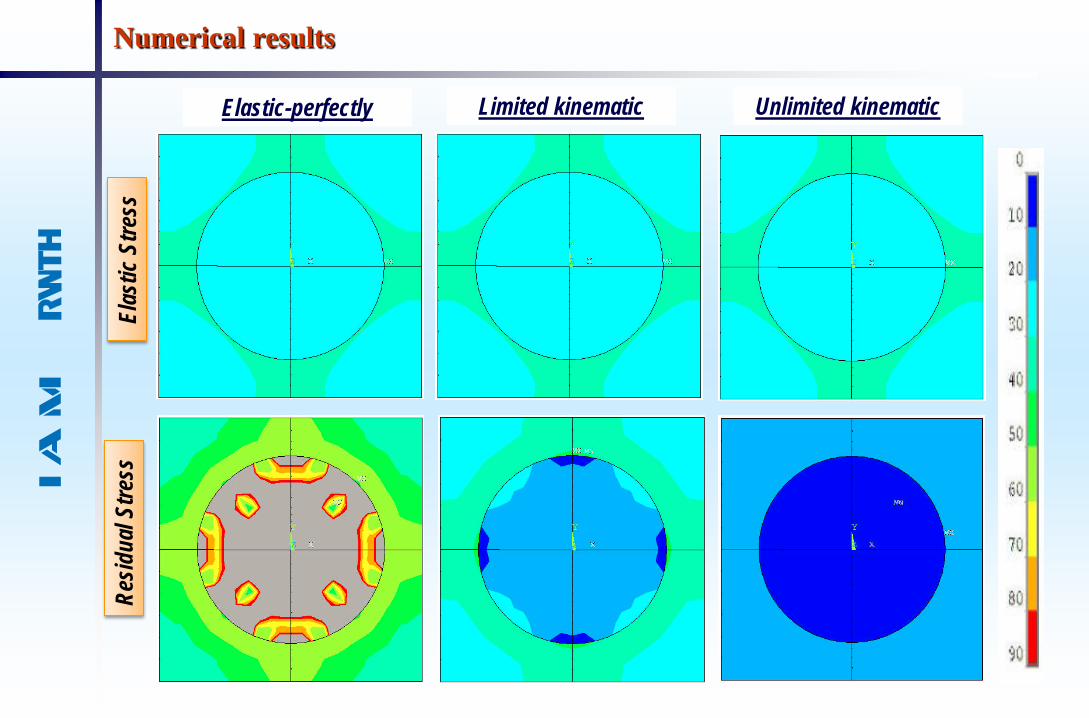
Numerical results

Limited kinematic Unlimited kinematic El

astic

Stre

ss

Elastic-perfectly Re

sidua

l Stre

ss

Numerical results

Limited kinematic Unlimited kinematic Ba

ck S

tress

Elastic-perfectly

Tota

l Stre

ss

CONCLUSIONS

Summary

Perspectives

• Application of a 3D nonconforming element to the limit and shakedown analysis of composites.

• Prediction of transverse elastic material properties of unidirectional continuous fiber reinforced metal matrix composites based on homogenization theory.

• Definition of yield loci for periodic composites and the prediction of plastic material properties by using yield surface fitting.

• Consideration of the hardening enlarged the shakedown domain. Different material model, different mechanism.

• Apply direct methods to other composites types and more complex problems.

• The general quantitative yield criterion fitting according to limit domain is still not solved yet.

• The presented results for the fiber-reinforced composite are only numerical, and a future effort has to be made in order to compare with experimental results quantitatively.

Thanks for

your attention!