Progress in Physics, 4/2007
122
ISSUE 2007 PROGRESS IN PHYSICS VOLUME 4 ISSN 1555-5534
description
Publications on advanced studies in theoretical and experimental physics, including related themes from mathematics.
Transcript of Progress in Physics, 4/2007
ISSUE 2007
PROGRESS
IN PHYSICS
VOLUME 4
ISSN 1555-5534
The Journal on Advanced Studies in Theoretical and Experimental Physics, including Related Themes from Mathematics
PROGRESS IN PHYSICSA quarterly issue scientific journal, registered with the Library of Congress (DC, USA). This journal is peer reviewed and included in the ab-stracting and indexing coverage of: Mathematical Reviews and MathSciNet (AMS, USA), DOAJ of Lund University (Sweden), Zentralblatt MATH(Germany), Referativnyi Zhurnal VINITI (Russia), etc.
To order printed issues of this journal, con-tact the Editors.
Electronic version of this journal can bedownloaded free of charge from the web-resources:http://www.ptep-online.comhttp://www.geocities.com/ptep online
Chief Editor
Dmitri [email protected]
Associate Editors
Florentin [email protected] [email protected] J. [email protected]
Postal address for correspondence:
Chair of the Departmentof Mathematics and Science,University of New Mexico,200 College Road,Gallup, NM 87301, USA
Copyright c© Progress in Physics, 2007
All rights reserved. Any part of Progressin Physics howsoever used in other publica-tions must include an appropriate citation ofthis journal.
Authors of articles published in Progress inPhysics retain their rights to use their ownarticles in any other publications and in anyway they see fit.
This journal is powered by LATEX
A variety of books can be downloaded freefrom the Digital Library of Science:http://www.gallup.unm.edu/�smarandache
ISSN: 1555-5534 (print)ISSN: 1555-5615 (online)
Standard Address Number: 297-5092Printed in the United States of America
OCTOBER 2007 VOLUME 4
CONTENTS
N. Stavroulakis On the Gravitational Field of a Pulsating Source . . . . . . . . . . . . . . . . . . . . . . . 3
R. T. Cahill Dynamical 3-Space: Supernovae and the Hubble Expansion — the OlderUniverse without Dark Energy . . . . . . . . . . . . . . . . . . . . . . . . . . . . . . . . . . . . . . . . . . . . . . . . . 9
R. T. Cahill Dynamical 3-Space: Alternative Explanation of the “Dark Matter Ring” . . . . 13
W. A. Zein, A. H. Phillips and O. A. Omar Quantum Spin Transport in MesoscopicInterferometer . . . . . . . . . . . . . . . . . . . . . . . . . . . . . . . . . . . . . . . . . . . . . . . . . . . . . . . . . . . . . . . 18
R. Carroll Some Remarks on Ricci Flow and the Quantum Potential . . . . . . . . . . . . . . . . . . . 22
P.-M. Robitaille The Little Heat Engine: Heat Transfer in Solids, Liquids and Gases . . . . 25
I. Suhendro A Four-Dimensional Continuum Theory of Space-Time and the ClassicalPhysical Fields . . . . . . . . . . . . . . . . . . . . . . . . . . . . . . . . . . . . . . . . . . . . . . . . . . . . . . . . . . . . . . 34
I. Suhendro A New Semi-Symmetric Unified Field Theory of the Classical Fields ofGravity and Electromagnetism . . . . . . . . . . . . . . . . . . . . . . . . . . . . . . . . . . . . . . . . . . . . . . . . 47
R. T. Cahill Optical-Fiber Gravitational Wave Detector: Dynamical 3-Space TurbulenceDetected . . . . . . . . . . . . . . . . . . . . . . . . . . . . . . . . . . . . . . . . . . . . . . . . . . . . . . . . . . . . . . . . . . . . 63
S. J. Crothers On the “Size” of Einstein’s Spherically Symmetric Universe . . . . . . . . . . . . . 69
P.-M. Robitaille On the Nature of the Microwave Background at the Lagrange 2 Point.Part I . . . . . . . . . . . . . . . . . . . . . . . . . . . . . . . . . . . . . . . . . . . . . . . . . . . . . . . . . . . . . . . . . . . . . . . 74
L. Borissova and D. Rabounski On the Nature of the Microwave Background at the La-grange 2 Point. Part II . . . . . . . . . . . . . . . . . . . . . . . . . . . . . . . . . . . . . . . . . . . . . . . . . . . . . . . . 84
I. Suhendro A New Conformal Theory of Semi-Classical Quantum General Relativity . . 96
B. Lehnert Joint Wave-Particle Properties of the Individual Photon . . . . . . . . . . . . . . . . . . . 104
V. Christianto and F. Smarandache A New Derivation of Biquaternion SchrodingerEquation and Plausible Implications . . . . . . . . . . . . . . . . . . . . . . . . . . . . . . . . . . . . . . . . . . 109
V. Christianto and F. Smarandache Thirty Unsolved Problems in the Physics of Elem-entary Particles . . . . . . . . . . . . . . . . . . . . . . . . . . . . . . . . . . . . . . . . . . . . . . . . . . . . . . . . . . . . . 112
LETTERS
J. Dunning-Davies Charles Kenneth Thornhill (1917–2007) . . . . . . . . . . . . . . . . . . . . . . . . . 115
P.-M. Robitaille Max Karl Ernst Ludwig Planck (1858–1947) . . . . . . . . . . . . . . . . . . . . . . . 117
Information for Authors and Subscribers
Progress in Physics has been created for publications on advanced studies intheoretical and experimental physics, including related themes from mathe-matics and astronomy. All submitted papers should be professional, in goodEnglish, containing a brief review of a problem and obtained results.
All submissions should be designed in LATEX format using Progress inPhysics template. This template can be downloaded from Progress in Physicshome page http://www.ptep-online.com. Abstract and the necessary informa-tion about author(s) should be included into the papers. To submit a paper,mail the file(s) to the Editor-in-Chief.
All submitted papers should be as brief as possible. We usually acceptbrief papers, no larger than 8–10 typeset journal pages. Short articles arepreferable. Large papers can be considered in exceptional cases to the sec-tion Special Reports intended for such publications in the journal. Lettersrelated to the publications in the journal or to the events among the sciencecommunity can be applied to the section Letters to Progress in Physics.
All that has been accepted for the online issue of Progress in Physics isprinted in the paper version of the journal. To order printed issues, contactthe Editors.
This journal is non-commercial, academic edition. It is printed from pri-vate donations. (Look for the current author fee in the online version of thejournal.)
October, 2007 PROGRESS IN PHYSICS Volume 4
On the Gravitational Field of a Pulsating Source
Nikias StavroulakisSolomou 35, 15233 Chalandri, Greece
E-mail: [email protected]
Because of the pseudo-theorem of Birkhoff, the important problem related to the dy-namical gravitational field of a non-stationary spherical mass is ignored by the rel-ativists. A clear formulation of this problem appears in the paper [5], which dealsalso with the establishment of the appropriate form of the spacetime metric. In thepresent paper we establish the corresponding equations of gravitation and bring outtheir solutions.
1 Introduction
As is shown in the paper [5], the propagation of gravitationfrom a spherical pulsating source is governed by a function�(t; �), termed propagation function, satisfying the followingconditions
@�(t; �)@t
> 0;@�(t; �)@�
6 0; �(t; �(t)) = t;
where �(t) denotes the time-dependent radius of the spherebounding the matter. The propagation function is not unique-ly defined. Any function fulfilling the above conditions char-acterizes the propagation of gravitation according to the fol-lowing rule: If the gravitational disturbance reaches thesphere kxk = � at the instant t, then � = �(t; �) is the instantof its radial emission from the entirety of the sphere boundingthe matter. Among the infinity of possible choices of �(t; �),we distinguish principally the one identified with the time co-ordinate, namely the propagation function giving rise to thecanonical �(4)-invariant metric
ds2 =�f(�; �)d� + `(�; �)
xdx�
�2�
���g(�; �)�
�2dx2+
��`(�; �)
�2��g(�; �)�
�2�(xdx)2
�2
� (1.1)
(here � denotes the time coordinate instead of the notation uused in the paper [5]).
Any other �(4)-invariant metric results from (1.1) if wereplace � by a conveniently chosen propagation function�(t; �). Consequently the general form of a �(4)-invariantmetric outside the matter can be written as
ds2 =��f��(t; �); �
�@�(t; �)@t
�dt+
+�f��(t; �); �
�@�(t; �)@�
+ `��(t; �); �
��xdx�
�2
�
���
g��(t; �); �
��
�2dx2 +
��`(�(t; �); �)
�2���g��(t; �); �
��
�2� (xdx)2
�2
�:
(1.2)
The equations of gravitation related to (1.2) are very com-plicated, but we do not need to write them explicitly, becausethe propagation function occurs in them as an arbitrary func-tion. So their solution results from that of the equations re-lated to (1.1) if we replace � by a general propagation func-tion �(t; �). It follows that the investigation of the �(4)-invariant gravitational field must by based on the canonicalmetric (1.1). The metric (1.2) indicates the dependence ofthe gravitational field upon the general propagation function�(t; �), but it is of no interest in dealing with specific prob-lems of gravitation for the following reason. Each allowablepropagation function is connected with a certain conceptionof time, so that the infinity of allowable propagation functionsintroduces an infinity of definitions of time with respect to thegeneral �(4)-invariant metric. This is why the notion of timeinvolved in (1.2) is not clear.
On the other hand, the notion of time related to the canon-ical metric, although unusual, is uniquely defined and concep-tually easily understandable.
This being said, from now on we will confine ourselves tothe explicit form of the canonical metric, namely
ds2 =�f(�; �)
�2d� 2 + 2f(�; �) `(�; �)(xdx)�
d� �
��g(�; �)�
�2dx2 +
�g(�; �)�
�2 (xdx)2
�2
(1.3)
which brings out its components:
g00 =�f(�; �)
�2; g0i = f(�; �) `(�; �)xi�;
gii = ��g(�; �)�
�2+�g(�; �)�
�2 x2i�2 ;
gij =�g(�; �)�
�2 xixj�2 ; (i; j = 1; 2; 3; i , j) :
Note that, since the canonical metric, on account of itsown definition, is conceived outside the matter, we have notto bother ourselves about questions of differentiability on thesubspace R � f(0; 0; 0)g of R � R3. It will be always un-derstood that the spacetime metric is defined for (�; �) 2 U ,� = kxk, U being the closed set f(�; �) 2 R2j� � �(� )g.
N. Stavroulakis. On the Gravitational Field of a Pulsating Source 3
Volume 4 PROGRESS IN PHYSICS October, 2007
2 Summary of auxiliary results
We recall that the Christoffel symbols of second kind relatedto a given �(4)-invariant spacetime metric [3] are the com-ponents of a �(4)-invariant tensor field and depend on tenfunctions B� = B�(t; �), (� = 0; 1; : : : ; 9), according to thefollowing formulae
�000 = B0; �0
0i = �0i0 = B1xi ; �i00 = B2xi ;
�0ii = B3 +B4x2
i ; �0ij = �0
ji = B4xixj ;
�ii0 = �i0i = B5 +B6x2i ; �ij0 = �i0j = B6xixj ;
�iii = B7x3i + (B8 + 2B9)xi ;
�ijj = B7xix2j +B8xi ; �jij = �jji = B7xix2
j +B9xi ;
�ijk = B7xixjxk ; (i; j; k = 1; 2; 3; i , j , k , i) :
We recall also that the corresponding Ricci tensor is asymmetric �(4)-invariant tensor defined by four functionsQ00, Q01, Q11, Q22, the computation of which is carriedout by means of the functions B� occurring in the Christoffelsymbols:
Q00 =@@t
(3B5 + �2B6)� �@B2
@��
�B2(3 + 4�2B9 � �2B1 + �2B8 + �2B7)�� 3B0B5 + 3B2
5 + �2B6(�B0 + 2B5 + �2B6) ;
Q01 =@@t
(�2B7 +B8 + 4B9)� 1�@B5
@�� �@B6
@�+
+B2(B3 + �2B4)� 2B6(2 + �2B9)��B1(3B5 + �2B6) ;
Q11 = �@B3
@t� �@B8
@�� (B0 +B5 + �2B6)B3 +
+ (1� �2B8)(B1 + �2B7 +B8 + 2B9)� 3B8 ;
Q22 = �@B4
@t+
1�@@�
(B1 +B8 + 2B9) +B21 +B2
8 �� 2B2
9 � 2B1B9 + 2B3B6 + (�B0 �B5 + �2B6)B4 +
+��3 + �2(�B1 +B8 � 2B9)
�B7 :
3 The Ricci tensor related to the canonical metric (1.3)
In order to find out the functions B�, (� = 0; 1; : : : ; 9), re-sulting from the metric (1.3), we have simply to write downthe explicit expressions of the Christoffel symbols �0
00, �001,
�100, �0
11, �101, �1
12, �122, thus obtaining
B0 =1f@f@�
+1`@`@�� 1`@f@�
; B1 = 0 ;
B2 = � f�`2
@`@�
+f�`2
@f@�
;
B3 =g
�2f`@g@�; B4 = � g
�4f`@g@�;
B5 =1g@g@�
; B6 =1�2`
@f@�� 1�2g
@g@�
;
B7 = � g�5f`
@g@�
+1�3f
@f@�
+1�4 +
g�5`2
@g@�
+
+1�3`
@`@�� 2�3g
@g@�;
B8 =g
�3f`@g@�
+1�2 � g
�3`2@g@�;
B9 = � 1�2 +
1�g@g@�:
The conditions B1 = 0, B3 + �2B4 = 0 imply severalsimplifications. Moreover an easy computation gives
Q11 + �2Q22 = 2�@B9
@��
� 2(1 + �2B9)(B8 +B9 + �2B7) + 4B9:
Replacing now everywhere the functions B�,(� = 0; 1; : : : ; 9), by their expressions, we obtain the fourfunctions defining the Ricci tensor.
Proposition 3.1 The functions Q00, Q01, Q11, Q22 relatedto (1.3) are defined by the following formulae.
Q00 =1`@2f@�@�
� f`2@2f@�2 +
f`2
@2`@�@�
+2g@2g@� 2 �
� f`3@`@�
@`@�
+f`3@f@�
@`@�
+2f`2g
@`@�
@g@��
� 2f`2g
@f@�
@g@�� 2fg
@f@�
@g@�� 2`g@`@�
@g@�
+
+2`g@f@�
@g@�� 1f`@f@�
@f@�
;
(3.1)
�Q01 =@@�
�1f`@(f`)@�
�� @@�
�1`@f@�
�+
+2g@2g@�@�
� 2`g@f@�
@g@�;
(3.2)
�2Q11 = �1� 2gf`
@2g@�@�
+g`2@2g@�2 � 2
f`@g@�
@g@��
� g`3@`@�
@g@�
+1`2
�@g@�
�2+
gf`2
@f@�
@g@�;
(3.3)
4 N. Stavroulakis. On the Gravitational Field of a Pulsating Source
October, 2007 PROGRESS IN PHYSICS Volume 4
Q11 + �2Q22 =2g
�@2g@�2 � @g
@�1f`@(f`)@�
�: (3.4)
Note that from (3.1) and (3.2) we deduce the followinguseful relation
`Q00 � f�Q01 =2`g@2g@� 2 +
2f`g@`@�
@g@��
� 2`fg
@f@�
@g@�� 2g@`@�
@g@�
+2g@f@�
@g@�� 2f
g@2g@�@�
:(3.5)
4 Reducing the system of the equations of gravitation
In order to clarify the fundamental problems with a minimumof computations, we will assume that the spherical sourceis not charged and neglect the cosmological constant. Thecharge of the source and the cosmological constant do notadd difficulties in the discussion of the main problems, so thatthey may be considered afterwards.
Of course, the equations of gravitation outside the pulsat-ing source are obtained by writing simply that the Ricci tensorvanishes, namely
Q00 = 0 ; Q01 = 0 ; Q11 = 0 ; Q11 + �2Q22 = 0 :
The first equation Q00 = 0 is to be replaced by the equa-tion
`Q00 � f�Q01 = 0
which, on account of (3.5), is easier to deal with.This being said, in order to investigate the equations of
gravitation, we assume that the dynamical states of the gravi-tational field alternate with the stationary ones without diffu-sion of gravitational waves.
We begin with the equation Q11 + �2Q22 = 0, which, onaccount of (3.4), can be written as
@@�
�1f`@g@�
�= 0
so that@g@�
= �f`
where � is a function depending uniquely on the time � .Let us consider a succession of three intervals of time,
[�1; �2] ]�2; �3[ [�3; �4];
such that the gravitational field is stationary during[�1; �2] and [�3; �4] and dynamical during ]�2; �3[.
When � describes [�1; �2] and [�3; �4], the functions f , `,g depend uniquely on �, so that � reduces then necessarilyto a constant, which, according to the known theory of thestationary vacuum solutions, equals 1
c , c being the classicalconstant (which, in the present situation, does not representthe velocity of propagation of light in vacuum). It follows
that, if � depends effectively on � during ]�2; �3[, then it ap-pears as a boundary condition at finite distance, like the ra-dius and the curvature radius of the sphere bounding the mat-ter. However, we cannot conceive a physical situation relatedto such a boundary condition. So we are led to assume that� is a universal constant, namely 1
c , keeping this value evenduring the dynamical states of the gravitational field. How-ever, before accepting finally the universal constancy of �, itis convenient to investigate the equations of gravitation underthe assumption that � depends effectively on time during theinterval ]�2; �3[.
We first prove that � = �(� ) does not vanish in ]�2; �3[.We argue by contradiction, assuming that �(�0) = 0 for somevalue �02 ]�2; �3[. Then @g
@� and @2g@�2 = � @(f`)
@� vanish for
� = �0, whereas @2g@�@�=(f`)�0+� @(f`)
@� reduces to (f`)�0(�0)for � = �0. Consequently the equation �2Q11 = 0 reducesto the condition 1 + 2g�0(�0) = 0 whence �0(�0)< 0 (sinceg > 0). It follows that �(� ) is strictly decreasing on a certaininterval [�0� "; �0 + "]� ]�2; �3[, " > 0, so that �(� ) < 0 forevery � 2 ]�0; �0 + "]. Let �00 be the least upper bound of theset of values � 2 ]�0 + "; �3[ for which �(� ) = 0 (This valueexists because �(� ) = 1
c > 0 on [�3; �4]). Then �(�00) = 0and �(� ) > �00 for � > �00. But, according to what has justbeen proved, the condition �(�00) = 0 implies that �(� ) < 0on a certain interval ]�00; �00 + �], � > 0, giving a contra-diction. It follows that the function �(� ) is strictly positiveon ]�2; �3[, hence also on any interval of non-stationarity, andsince �(� ) = 1
c on the intervals of stationarity, it is strictlypositive everywhere. Consequently we are allowed to intro-duce the inverse function � = �(� ) = 1
�(�) and write
f` = �@g@�
(4.1)
andf =
�`@g@�: (4.2)
Inserting this expression of f into the equation �2Q11 = 0and then multiplying throughout by @g
@� , we obtain an equationwhich can be written as
@@�
�� 2g�@g@�
+g`2
�@g@�
�2� g�
= 0
whence
�2g�@g@�
+g`2
�@g@�
�2� g = �2� = function of �;
and@g@�
=�2
�� 1 +
2�g
+1`2
�@g@�
�2�: (4.3)
It follows that
@2g@�@�
= ��� �g2@g@�� 1`3@`@�
�@g@�
�2+
1`2@g@�
@2g@�2
�(4.4)
N. Stavroulakis. On the Gravitational Field of a Pulsating Source 5
Volume 4 PROGRESS IN PHYSICS October, 2007
and
@3g@�@�2 = �
�2�g3
�@g@�
�2� �g2@2g@�2 +
+3`4
�@`@�
�2�@g@�
�2� 1`3@2`@�2
�@g@�
�2�
� 4`3@`@�
@g@�
@2g@�2 +
1`2
�@2g@�2
�2+
1`2@g@�
@3g@�3
�:
(4.5)
On the other hand, since f` = �@g@� , the expression (3.2)is transformed as follows
�Q01 =1�@g@�
�2
�@g@�
@3g@�@�2 � @2g
@�2@2g@�@�
�+
+��� 3`4
�@`@�
�2 @g@�
+1`3@2`@�2
@g@�
+
+3`3@`@�
@2g@�2 � 1
`2@3g@�3 � 2�
g3@g@�
�and replacing in it @2g
@�@� and @3g@�@�2 by their expressions (4.4)
and (4.5), we find �Q01 = 0. Consequently the equation ofgravitation �Q01 = 0 is verified. It remains to examine theequation `Q00� f�Q01 = 0. We need some preliminarycomputations. First we consider the expression of @
2g@�2 result-
ing from the derivation of (4.3) with respect to � , and thenreplacing in it @g
@� and @2g@�@� by their expressions (4.3) and
(4.4), we obtain
2@2g@� 2 = �d�
d�+ 2
d�d�
�g
+1`2d�d�
�@g@�
�2+
+2�gd�d�� 2�2�2
g3 +�2�g2 � 2�
`3@`@�
�@g@�
�2�
� 3�2�`2g2
�@g@�
�2� 2�2
`5@`@�
�@g@�
�3+
2�2
`4
�@g@�
�2 @2g@�2 :
(4.6)
Next, because of (4.2), we have
@f@�
= � �`2@`@�
@g@�
+�`@2g@�2 (4.7)
and@f@�
=1`d�d�
@g@�� �`2@`@�
@g@�
+�`@2g@�@�
:
Lastly taking into account (4.4), we obtain
@f@�
=1`d�d�
@g@�� �`2@`@�
@g@�� �2�`g2
@g@��
� �2
`4@`@�
�@g@�
�2+�2
`3@g@�
@2g@�2 :
(4.8)
Now inserting (4.2), (4.3), (4.4), (4.6), (4.7), (4.8) into
(3.5), we obtain, after cancelations, the very simple expres-sion
`Q00 � f�Q01 =2�`g2
d�d�
:
Consequently the last equation of gravitation, namely`Q00� f�Q01 = 0, implies that d�
d� = 0, namely that � re-duces to a constant.
Finally the system of the equations of gravitation is re-duced to a system of two equations, namely (4.1) and (4.3),where � is a constant valid whatever is the state of the field,and � is a strictly positive function of time reducing to theconstant c during the stationary states of the field. As alreadyremarked, if � depends effectively on � during the dynamicalstates, then it plays the part of a boundary condition the ori-gin of which is indefinable. The following reasoning, whichis allowed according to the principles of General Relativity,corroborates the idea that � must be taken everywhere equalto c.
Since �(� )> 0 everywhere, we can introduce the newtime coordinate
u =1c
Z �
�0�(v)dv
which amounts to a change of coordinate in the sphere bound-ing the matter. The function
(� ) =1c
Z �
�0�(v)dv
being strictly increasing, its inverse � ='(u) is well definedand '0= 1
0 = c� . Instead of `(�; �) and g(�; �) we have now
the functions L(u; �) = `('(u); �) andG(u; �) = g('(u); �),Moreover, since fd� = f'0du, f(�; �) is replaced by the
function F (u; �) ='0(u)f('(u); �) = c�f('(u); �).
It follows that
FL = '0f` =c��@g@�
= c@G@�
(4.9)
and
@G@u
=@g@�
d�du
=�2
�� 1 +
2�g
+1`2
�@g@�
�2� c�
=
=c2
�� 1 +
2�G
+1L2
�@G@�
�2�:
(4.10)
Writing again f(�; �), `(�; �), g(�; �) respectively insteadof F (u; �), L(u; �), G(u; �), we see that the equations (4.9)and (4.10) are rewritten as
f` = c@g@�
(4.11)
@g@�
=c2
�� 1 +
2�g
+1`2
�@g@�
�2�: (4.12)
So (4.1) and (4.3) preserve their form, but the function �is now replaced by the constant c. Finally we are allowed todispense with the function � and deal subsequently with theequations (4.11) and (4.12).
6 N. Stavroulakis. On the Gravitational Field of a Pulsating Source
October, 2007 PROGRESS IN PHYSICS Volume 4
5 Stationary and non-stationary solutions
If the field is stationary during a certain interval of time, thenthe derivative @g
@� vanishes on this interval. The converseis also true. In order to clarify the situation, consider thesuccession of three intervals of time ]�1; �2[, [�2; �3], ]�3; �4[such that ]�1; �2[ and ]�3; �4[ be maximal intervals of non-stationarity, and @g
@� = 0 on [�2; �3]. Then we have on [�2; �3]the equation
�1 +2�g
+1`2
�@g@�
�2= 0
from which it follows that ` does not depend either on � . Onaccount of (4.11), this property is also valid for f . Conse-quently the vanishing of @g
@� on [�2; �3] implies the establish-ment of a stationary state.
During the stationary state we are allowed to introducethe radial geodesic distance
� =Z �
0`(v)dv
and investigate subsequently the stationary equations in ac-cordance with the exposition appearing in the paper [4]. Since
� = �(�)
is a strictly increasing function of �, the inverse function�= (�) is well defined and allows to consider as functionof � every function of �. In particular the curvature radiusG(�) = g ( (�)) appears as a function of the geodesic dis-tance � and gives rise to a complete study of the stationaryfield. From this study it follows that the constant � equalskmc2 and that the solution G(�) possesses the greatest lower
bound 2�. Moreover G(�) is defined by the equationZ G
2�
duq1� 2�
u
= � � �0 (5.1)
where �0 is a new constant unknown in the classical theory ofgravitation. This constant is defined by means of the radius �1and the curvature radius �1 = G(�1) of the sphere boundingthe matter:
�0 = �1 � pG(�1)(G(�1)� 2�)�
� 2� ln
sG(�1)
2�+
sG(�1)
2�� 1
!:
So the values �1 and �1 =G(�1) constitute the boundaryconditions at finite distance. Regarding F =F (�) = f( (�)),it is defined by means of G:
F = cG0 = cr
1� 2�G; (G > 2�) :
The so obtained solution does not extend beyond the in-terval [�2; �3] and even its validity for � = �2 and � = �3 is
questionable. The notion of radial geodesic distance does notmake sense in the intervals of non-stationarity such as ]�1; �2[and ]�3; �4[. Then the integralZ �
0`(�; v)dv
depends on the time � and does not define an invariant length.As a way out of the difficulty we confine ourselves to theconsideration of the radical coordinate related to the manifolditself, namely �=kxk.
Regarding the curvature radius �(� ), it is needed in orderto conceive the solution of the equations of gravitation. Thefunction g(�; �) must be so defined that g (�; �(� )) = �(� ).The functions �(� ) and �(� ) are the boundary conditions atfinite distance for the non-stationary field. They are not di-rectly connected with the boundary conditions of the station-ary field defined by means of the radial geodesic distance.
6 On the non-stationary solutions
According to very strong arguments summarized in the paper[2], the relation g > 2� is always valid outside the matterwhatever is the state of the field. This is why the first attemptto obtain dynamical solutions was based on an equation anal-ogous to (5.1), namelyZ g
2�
duq1� 2�
u
= (�; �)
where (�; �) is a new function satisfying certain con-ditions. This idea underlies the results presented briefly inthe paper [1]. However the usefulness of introduction of anew function is questionable. It is more natural to deal di-rectly with the functions f , `, g involved in the metric. Inany case we have to do with two equations, namely (4.11)and (4.12), so that we cannot expect to define completely thethree unknown functions. Note also that, even in the con-sidered stationary solution, the equation (5.1) does not de-fine completely the function G on account of the new un-known constant �0. In the general case there is no way todefine the function g(�; �) by means of parameters and sim-pler functions. The only available equation, namely (4.12), apartial differential equation including the unknown function`(�; �), is, in fact, intractable. As a way out of the difficulties,we propose to consider the function g(�; �) as a new entityrequired by the non-Euclidean structure involved in the dy-namical gravitational field. In the present state of our knowl-edge, we confine ourselves to put forward the main featuresof g(�; �) in the closed set
U = f(�; �) 2 R2j� > �(� )g:Since the vanishing of f or ` would imply the degeneracyof the spacetime metric, these two functions are necessarilystrictly positive on U . Then from the equation (4.11) it fol-
N. Stavroulakis. On the Gravitational Field of a Pulsating Source 7
Volume 4 PROGRESS IN PHYSICS October, 2007
lows that@g (�; �)@�
> 0 (6.1)
on the closed set U . On the other hand, since (4.12) can berewritten as
2c@g@�
+ 1� 2�g
=1`2
�@g@�
�2we have also
2c@g@�
+ 1� 2�g> 0 (6.2)
on the closed set U . Now, on account of (6.1) and (6.2), theequations (4.11) and (4.12) define uniquely the functions fand ` by means of g:
f = c
s2c@g@�
+ 1� 2�g
(6.3)
` =@g=@�q
2c@g@� + 1� 2�
g
: (6.4)
It is now obvious that the curvature radius g (�; �) playsthe main part in the conception of the gravitational field. Al-though it has nothing to do with coordinates, the relativistshave reduced it to a so-called radial coordinate from the be-ginnings of General Relativity. This glaring mistake has givenrise to intolerable misunderstandings and distorted complete-ly the theory of the gravitational field.
Let ]�1; �2[ be a maximal bounded open interval of non-stationarity. Then @g
@� = 0 for � = �1 and � = �2, but @g@� , 0on an open dense subset of ]�1; �2[. So @g
@� appears as a gravi-tational wave travelling to infinity, and it is natural to assumethat @g
@� tends uniformly to zero on [�1; �2] as �!+1. Ofcourse the behaviour of @g
@� depends on the boundary condi-tions which do not appear in the obtained general solution.They are to be introduced in accordance with the envisagedproblem. In any case the gravitational disturbance plays thefundamental part in the conception of the dynamical gravita-tion, but the state of the field does not follow always a simplerule.
In particular, if the gravitational disturbance vanishes dur-ing a certain interval of time [�1; �2], the function g(�; �) doesnot depend necessarily only on � during [�1; �2]. In otherwords, the gravitational field does not follow necessarily theHuyghens principle contrary to the solutions of the classicalwave equation in R3.
We deal briefly with the case of a Huyghens type field,namely a �(4)-invariant gravitational field such that the van-ishing of the gravitational disturbance on a time interval im-plies the establishment of a universal stationary state. Thenthe time is involved in the curvature radius by means of theboundary conditions �(� ), �(� ), so that g(�; �) is in fact afunction of (� (� ); � (� ); �) : g (�(� ); � (� ); �). The corres-
ponding expressions for f and ` result from (6.3) and (6.4):
f = c
s2c
�@g@�
�0(� ) +@g@�
� 0(� )�
+ 1� 2�g
` =@g@�r
2c
�@g@� �
0(� ) + @g@� �
0(� )�
+ 1� 2�g
where g denotes g(�(� ); �(� ); �).If �0(� ) = � 0(� ) = 0 during an interval of time, the bound-
ary conditions �(� ), �(� ) reduce to positive constants �0, �0on this interval, so that the curvature radius defining the sta-tionary states depends on the constants �0; �0 : g(�0; �0; �). Itis easy to write down the conditions satisfied by g(�0; �0; �),considered as function of three variables.
Submitted on June 12, 2007Accepted on June 13, 2007
References
1. Stavroulakis N. Exact solution for the field of a pulsatingsource. Abstracts of Contributed Papers for the DiscussionGroups, 9th International Conference on General Relativityand Gravitation, July 14–19, 1980, Jena, Volume 1, 74–75.
2. Stavroulakis N. Particules et particules test en relativitegenerale. Annales Fond. Louis de Broglie, 1991, v. 16, No. 2,129–175.
3. Stavroulakis N. Verite scientifique et trous noirs (troisieme par-tie) Equations de gravitation relatives a une metrique �(4)-invariante. Annales Fond. Louis de Broglie, 2001, v. 26, No. 4,605–631.
4. Stavroulakis N. Non-Euclidean geometry and gravitation.Progress in Physics, 2006, v. 2, 68–75.
5. Stavroulakis N. On the propagation of gravitation from a pul-sating source. Progress in Physics, 2007, v. 2, 75–82.
8 N. Stavroulakis. On the Gravitational Field of a Pulsating Source
October, 2007 PROGRESS IN PHYSICS Volume 4
Dynamical 3-Space: Supernovae and the Hubble Expansion — the OlderUniverse without Dark Energy
Reginald T. Cahill
School of Chemistry, Physics and Earth Sciences, Flinders University, Adelaide 5001, AustraliaE-mail: [email protected]
We apply the new dynamics of 3-space to cosmology by deriving a Hubble expansionsolution. This dynamics involves two constants; G and � — the fine structure constant.This solution gives an excellent parameter-free fit to the recent supernova and gamma-ray burst redshift data without the need for “dark energy” or “dark matter”. The dataand theory together imply an older age for the universe of some 14.7Gyrs. The 3-spacedynamics has explained the bore hole anomaly, spiral galaxy flat rotation speeds, themasses of black holes in spherical galaxies, gravitational light bending and lensing, allwithout invoking “dark matter” or “dark energy”. These developments imply that a newunderstanding of the universe is now available.
1 Introduction
There are theoretical claims based on observations of Type Iasupernova (SNe Ia) redshifts [1, 2] that the universe expan-sion is accelerating. The cause of this acceleration has beenattributed to an undetected “dark energy”. Here the dynami-cal theory of 3-space is applied to Hubble expansion dynam-ics, with the result that the supernova and gamma-ray burstredshift data is well fitted without an acceleration effect andwithout the need to introduce any notion of “dark energy”.So, like “dark matter”, “dark energy” is an unnecessary andspurious notion. These developments imply that a new under-standing of the universe is now available.
1.1 Dynamical 3-Space
At a deeper level an information-theoretic approach to mod-elling reality, Process Physics [3, 4], leads to an emergentstructured “space” which is 3-dimensional and dynamic, butwhere the 3-dimensionality is only approximate, in that if weignore non-trivial topological aspects of the space, then it maybe embedded in a 3-dimensional geometrical manifold. Herethe space is a real existent discrete fractal network of relation-ships or connectivities, but the embedding space is purely amathematical way of characterising the 3-dimensionality ofthe network. Embedding the network in the embedding spaceis very arbitrary; we could equally well rotate the embeddingor use an embedding that has the network translated or trans-lating. These general requirements then dictate the minimaldynamics for the actual network, at a phenomenological level.To see this we assume at a coarse grained level that the dy-namical patterns within the network may be described by avelocity field v(r; t), where r is the location of a small regionin the network according to some arbitrary embedding. The3-space velocity field has been observed in at least 8 exper-iments [3, 4]. For simplicity we assume here that the globaltopology of the network is not significant for the local dynam-
ics, and so we embed in anE3, although a generalisation to anembedding in S3 is straightforward and might be relevant tocosmology. The minimal dynamics is then obtained by writ-ing down the lowest-order zero-rank tensors, of dimension1=t2, that are invariant under translation and rotation, giving
r��@v@t
+ (v�r)v�
+�8�(trD)2�tr(D2)
�=�4�G�; (1)
Dij =12
�@vi@xj
+@vj@xi
�; (2)
where �(r; t) is the effective matter density. The embeddingspace coordinates provide a coordinate system or frame ofreference that is convenient to describing the velocity field,but which is not real. In Process Physics quantum matter aretopological defects in the network, but here it is sufficient togive a simple description in terms of an effective density. Gis Newton’s gravitational constant, and describes the rate ofnon-conservative flow of space into matter, and data from thebore hole g anomaly and the mass spectrum of black holesreveals that � is the fine structure constant �1/137, to withinexperimental error [5, 6, 7].
Now the acceleration a of the dynamical patterns in the3-space is given by the Euler or convective expression
a(r; t) = lim�t!0
v�r + v(r; t)�t; t+ �t
�� v(r; t)�t
=
=@v@t
+ (v � r)v :(3)
As shown in [8] the acceleration g of quantum matter isidentical to the acceleration of the 3-space itself, apart fromvorticity and relativistic effects, and so the gravitational ac-celeration of matter is also given by (3). Eqn. (1) has blackhole solutions for which the effective masses agree with ob-servational data for spherical star systems [5, 6, 7]. The-ses black holes also explain the flat rotation curves in spiralgalaxies [9].
R. T. Cahill. Dynamical 3-Space: Supernovae and the Hubble Expansion — the Older Universe without Dark Energy 9
Volume 4 PROGRESS IN PHYSICS October, 2007
2 Supernova and gamma-ray burst data
The supernovae and gamma-ray bursts provide standard can-dles that enable observation of the expansion of the universe.The supernova data set used herein and shown in Figs. 2 and3 is available at [10]. Quoting from [10] we note that Davis etal. [11] combined several data sets by taking the ESSENCEdata set from Table 9 of Wood–Vassey et al. (2007) [13],using only the supernova that passed the light-curve-fit qual-ity criteria. They took the HST data from Table 6 of Riesset al. (2007) [12], using only the supernovae classified asgold. To put these data sets on the same Hubble diagramDavis et al. used 36 local supernovae that are in common be-tween these two data sets. When discarding supernovae withz < 0.0233 (due to larger uncertainties in the peculiar veloci-ties) they found an offset of 0.037�0.021 magnitude betweenthe data sets, which they then corrected for by subtracting thisconstant from the HST data set. The dispersion in this offsetwas also accounted for in the uncertainties. The HST dataset had an additional 0.08 magnitude added to the distancemodulus errors to allow for the intrinsic dispersion of the su-pernova luminosities. The value used by Wood–Vassey et al.(2007) [13] was instead 0.10 mag. Davis et al. adjusted forthis difference by putting the Gold supernovae on the samescale as the ESSENCE supernovae. Finally, they also addedthe dispersion of 0.021 magnitude introduced by the simpleoffset described above to the errors of the 30 supernovae in theHST data set. The final supernova data base for the distancemodulus �obs(z) is shown in Figs. 2 and 3. The gamma-rayburst (GRB) data is from Schaefer [14].
3 Expanding 3-space — the Hubble solution
Suppose that we have a radially symmetric density �(r; t) andthat we look for a radially symmetric time-dependent flowv(r; t) = v(r; t)r from (1). Then v(r; t) satisfies the equation,with v0= @v(r;t)
@r ,
@@t
�2vr
+ v0�
+ vv00 + 2vv0r
+ (v0)2 +
+�4
�v2
r2 +2vv0r
�= �4�G�(r; t) :
(4)
Consider first the zero energy case �= 0. Then we havea Hubble solution v(r; t) =H(t)r, a centreless flow, deter-mined by
_H +�
1 +�4
�H2 = 0 (5)
with _H = dHdt . We also introduce in the usual manner the scale
factor R(t) according to H(t) = 1RdRdt . We then obtain the
solution
H(t) =1
(1 + �4 )t
= H0t0t
; R(t) = R0
�tt0
�4=(4+�)
(6)
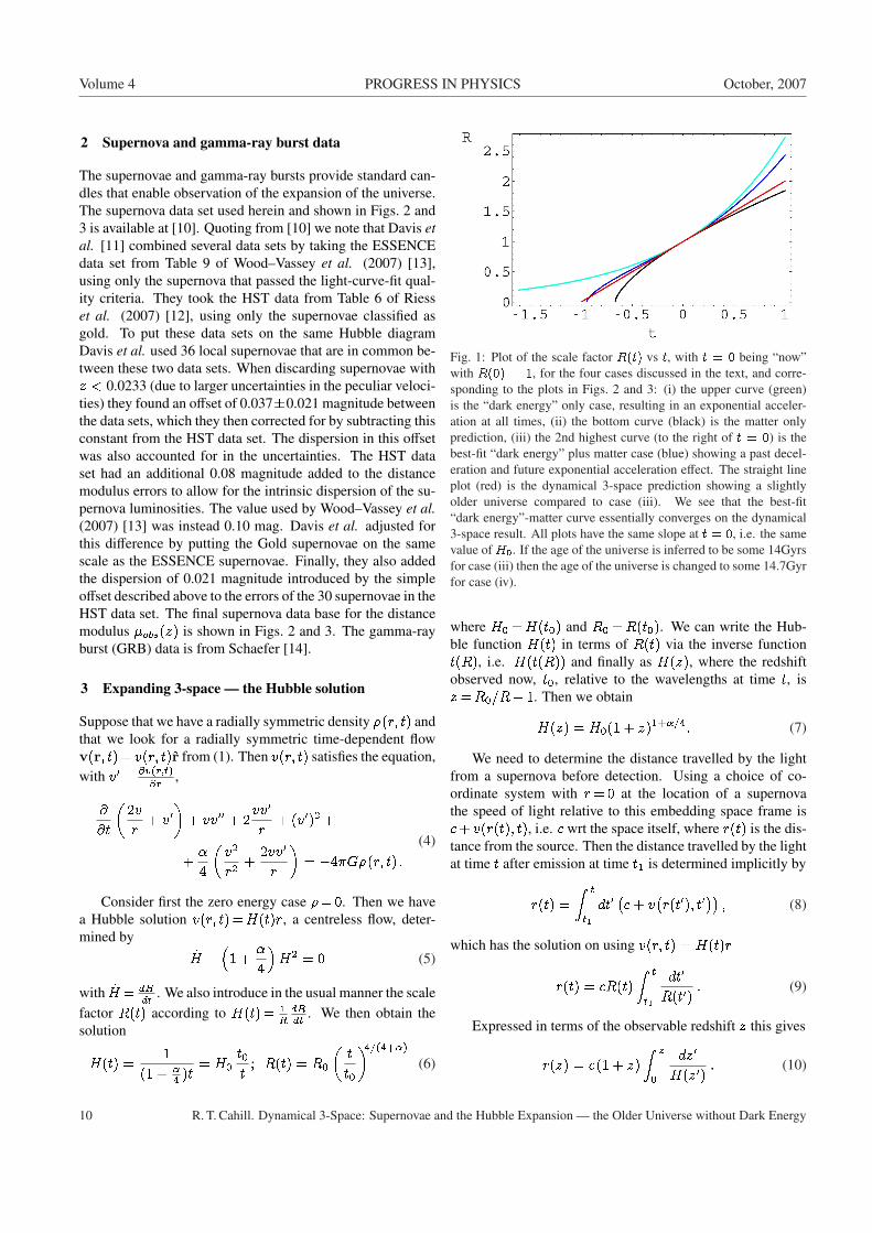
Fig. 1: Plot of the scale factor R(t) vs t, with t = 0 being “now”with R(0) = 1, for the four cases discussed in the text, and corre-sponding to the plots in Figs. 2 and 3: (i) the upper curve (green)is the “dark energy” only case, resulting in an exponential acceler-ation at all times, (ii) the bottom curve (black) is the matter onlyprediction, (iii) the 2nd highest curve (to the right of t = 0) is thebest-fit “dark energy” plus matter case (blue) showing a past decel-eration and future exponential acceleration effect. The straight lineplot (red) is the dynamical 3-space prediction showing a slightlyolder universe compared to case (iii). We see that the best-fit“dark energy”-matter curve essentially converges on the dynamical3-space result. All plots have the same slope at t = 0, i.e. the samevalue ofH0. If the age of the universe is inferred to be some 14Gyrsfor case (iii) then the age of the universe is changed to some 14.7Gyrfor case (iv).
where H0 =H(t0) and R0 =R(t0). We can write the Hub-ble function H(t) in terms of R(t) via the inverse functiont(R), i.e. H(t(R)) and finally as H(z), where the redshiftobserved now, t0, relative to the wavelengths at time t, isz=R0=R� 1. Then we obtain
H(z) = H0(1 + z)1+�=4: (7)
We need to determine the distance travelled by the lightfrom a supernova before detection. Using a choice of co-ordinate system with r= 0 at the location of a supernovathe speed of light relative to this embedding space frame isc+ v(r(t); t), i.e. c wrt the space itself, where r(t) is the dis-tance from the source. Then the distance travelled by the lightat time t after emission at time t1 is determined implicitly by
r(t) =Z t
t1dt0�c+ v
�r(t0); t0
��; (8)
which has the solution on using v(r; t) = H(t)r
r(t) = cR(t)Z t
t1
dt0R(t0) : (9)
Expressed in terms of the observable redshift z this gives
r(z) = c(1 + z)Z z
0
dz0H(z0) : (10)
10 R. T. Cahill. Dynamical 3-Space: Supernovae and the Hubble Expansion — the Older Universe without Dark Energy
October, 2007 PROGRESS IN PHYSICS Volume 4
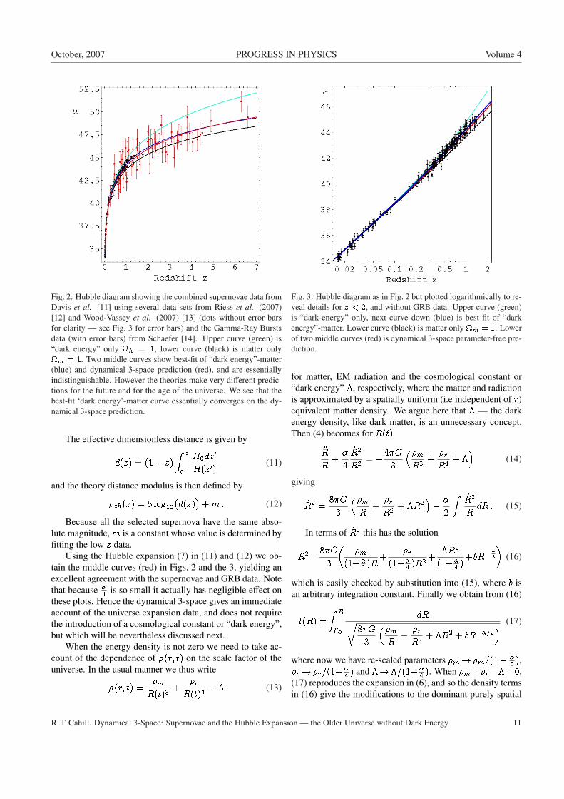
Fig. 2: Hubble diagram showing the combined supernovae data fromDavis et al. [11] using several data sets from Riess et al. (2007)[12] and Wood-Vassey et al. (2007) [13] (dots without error barsfor clarity — see Fig. 3 for error bars) and the Gamma-Ray Burstsdata (with error bars) from Schaefer [14]. Upper curve (green) is“dark energy” only � = 1, lower curve (black) is matter onlym = 1. Two middle curves show best-fit of “dark energy”-matter(blue) and dynamical 3-space prediction (red), and are essentiallyindistinguishable. However the theories make very different predic-tions for the future and for the age of the universe. We see that thebest-fit ‘dark energy’-matter curve essentially converges on the dy-namical 3-space prediction.
The effective dimensionless distance is given by
d(z) = (1 + z)Z z
0
H0dz0H(z0) (11)
and the theory distance modulus is then defined by
�th(z) = 5 log10�d(z)
�+m: (12)
Because all the selected supernova have the same abso-lute magnitude,m is a constant whose value is determined byfitting the low z data.
Using the Hubble expansion (7) in (11) and (12) we ob-tain the middle curves (red) in Figs. 2 and the 3, yielding anexcellent agreement with the supernovae and GRB data. Notethat because �
4 is so small it actually has negligible effect onthese plots. Hence the dynamical 3-space gives an immediateaccount of the universe expansion data, and does not requirethe introduction of a cosmological constant or “dark energy”,but which will be nevertheless discussed next.
When the energy density is not zero we need to take ac-count of the dependence of �(r; t) on the scale factor of theuniverse. In the usual manner we thus write
�(r; t) =�mR(t)3 +
�rR(t)4 + � (13)
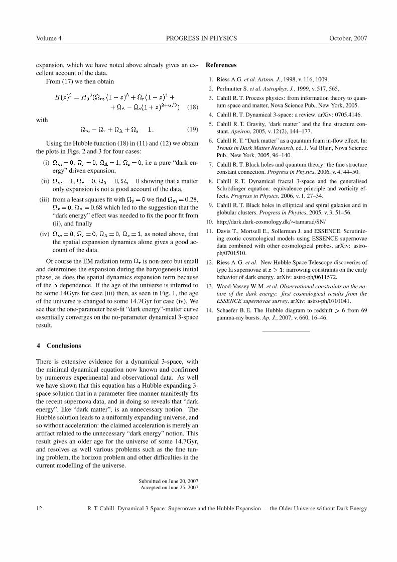
Fig. 3: Hubble diagram as in Fig. 2 but plotted logarithmically to re-veal details for z < 2, and without GRB data. Upper curve (green)is “dark-energy” only, next curve down (blue) is best fit of “darkenergy”-matter. Lower curve (black) is matter only m = 1. Lowerof two middle curves (red) is dynamical 3-space parameter-free pre-diction.
for matter, EM radiation and the cosmological constant or“dark energy” �, respectively, where the matter and radiationis approximated by a spatially uniform (i.e independent of r)equivalent matter density. We argue here that � — the darkenergy density, like dark matter, is an unnecessary concept.Then (4) becomes for R(t)
�RR
+�4
_R2
R2 = �4�G3
��mR3 +
�rR4 + �
�(14)
giving
_R2 =8�G
3
��mR
+�rR2 + �R2
�� �2
Z _R2
RdR : (15)
In terms of _R2 this has the solution
_R2 =8�G
3
��m
(1��2 )R+
�r(1��4 )R2 +
�R2
(1+�4 )
+bR��2�
(16)
which is easily checked by substitution into (15), where b isan arbitrary integration constant. Finally we obtain from (16)
t(R) =Z R
R0
dRr8�G
3
��mR
+�rR2 + �R2 + bR��=2
� (17)
where now we have re-scaled parameters �m! �m=(1� �2 ),
�r! �r=(1� �4 ) and �!�=(1+ �
4 ). When �m= �r=�= 0,(17) reproduces the expansion in (6), and so the density termsin (16) give the modifications to the dominant purely spatial
R. T. Cahill. Dynamical 3-Space: Supernovae and the Hubble Expansion — the Older Universe without Dark Energy 11
Volume 4 PROGRESS IN PHYSICS October, 2007
expansion, which we have noted above already gives an ex-cellent account of the data.
From (17) we then obtain
H(z)2 = H02(m (1 + z)3 + r(1 + z)4 +
+ � + s(1 + z)2+�=2) (18)
withm + r + � + s = 1 : (19)
Using the Hubble function (18) in (11) and (12) we obtainthe plots in Figs. 2 and 3 for four cases:
(i) m = 0, r = 0, � = 1, s = 0, i.e a pure “dark en-ergy” driven expansion,
(ii) m = 1, r = 0, � = 0, s = 0 showing that a matteronly expansion is not a good account of the data,
(iii) from a least squares fit with s = 0 we find m = 0.28,r = 0, � = 0.68 which led to the suggestion that the“dark energy” effect was needed to fix the poor fit from(ii), and finally
(iv) m = 0, r = 0, � = 0, s = 1, as noted above, thatthe spatial expansion dynamics alone gives a good ac-count of the data.
Of course the EM radiation term r is non-zero but smalland determines the expansion during the baryogenesis initialphase, as does the spatial dynamics expansion term becauseof the � dependence. If the age of the universe is inferred tobe some 14Gyrs for case (iii) then, as seen in Fig. 1, the ageof the universe is changed to some 14.7Gyr for case (iv). Wesee that the one-parameter best-fit “dark energy”-matter curveessentially converges on the no-parameter dynamical 3-spaceresult.
4 Conclusions
There is extensive evidence for a dynamical 3-space, withthe minimal dynamical equation now known and confirmedby numerous experimental and observational data. As wellwe have shown that this equation has a Hubble expanding 3-space solution that in a parameter-free manner manifestly fitsthe recent supernova data, and in doing so reveals that “darkenergy”, like “dark matter”, is an unnecessary notion. TheHubble solution leads to a uniformly expanding universe, andso without acceleration: the claimed acceleration is merely anartifact related to the unnecessary “dark energy” notion. Thisresult gives an older age for the universe of some 14.7Gyr,and resolves as well various problems such as the fine tun-ing problem, the horizon problem and other difficulties in thecurrent modelling of the universe.
Submitted on June 20, 2007Accepted on June 25, 2007
References
1. Riess A.G. et al. Astron. J., 1998, v. 116, 1009.
2. Perlmutter S. et al. Astrophys. J., 1999, v. 517, 565,.
3. Cahill R. T. Process physics: from information theory to quan-tum space and matter, Nova Science Pub., New York, 2005.
4. Cahill R. T. Dynamical 3-space: a review. arXiv: 0705.4146.
5. Cahill R. T. Gravity, ‘dark matter’ and the fine structure con-stant. Apeiron, 2005, v. 12(2), 144–177.
6. Cahill R. T. “Dark matter” as a quantum foam in-flow effect. In:Trends in Dark Matter Research, ed. J. Val Blain, Nova SciencePub., New York, 2005, 96–140.
7. Cahill R. T. Black holes and quantum theory: the fine structureconstant connection. Progress in Physics, 2006, v. 4, 44–50.
8. Cahill R. T. Dynamical fractal 3-space and the generalisedSchrodinger equation: equivalence principle and vorticity ef-fects. Progress in Physics, 2006, v. 1, 27–34.
9. Cahill R. T. Black holes in elliptical and spiral galaxies and inglobular clusters. Progress in Physics, 2005, v. 3, 51–56.
10. http://dark.dark-cosmology.dk/�tamarad/SN/
11. Davis T., Mortsell E., Sollerman J. and ESSENCE. Scrutiniz-ing exotic cosmological models using ESSENCE supernovaedata combined with other cosmological probes. arXiv: astro-ph/0701510.
12. Riess A. G. et al. New Hubble Space Telescope discoveries oftype Ia supernovae at z > 1: narrowing constraints on the earlybehavior of dark energy. arXiv: astro-ph/0611572.
13. Wood-Vassey W. M. et al. Observational constraints on the na-ture of the dark energy: first cosmological results from theESSENCE supernovae survey. arXiv: astro-ph/0701041.
14. Schaefer B. E. The Hubble diagram to redshift > 6 from 69gamma-ray bursts. Ap. J., 2007, v. 660, 16–46.
12 R. T. Cahill. Dynamical 3-Space: Supernovae and the Hubble Expansion — the Older Universe without Dark Energy
October, 2007 PROGRESS IN PHYSICS Volume 4
Dynamical 3-Space: Alternative Explanation of the “Dark Matter Ring”
Reginald T. Cahill
School of Chemistry, Physics and Earth Sciences, Flinders University, Adelaide 5001, AustraliaE-mail: [email protected]
NASA has claimed the discovery of a “Ring of Dark Matter” in the galaxy cluster CL0024+17, see Jee M.J. et al. arXiv:0705.2171, based upon gravitational lensing data.Here we show that the lensing can be given an alternative explanation that does notinvolve “dark matter”. This explanation comes from the new dynamics of 3-space. Thisdynamics involves two constant G and � — the fine structure constant. This dynamicshas explained the bore hole anomaly, spiral galaxy flat rotation speeds, the masses ofblack holes in spherical galaxies, gravitational light bending and lensing, all withoutinvoking “dark matter”, and also the supernova redshift data without the need for “darkenergy”.
1 Introduction
Jee et al. [1] claim that the analysis of gravitational lens-ing data from the HST observations of the galaxy cluster CL0024+17 demonstrates the existence of a “dark matter ring”.While the lensing is clearly evident, as an observable phe-nomenon, it does not follow that this must be caused by someundetected form of matter, namely the putative “dark matter”.Here we show that the lensing can be given an alternative ex-planation that does not involve “dark matter”. This explana-tion comes from the new dynamics of 3-space [2, 3, 4, 5, 6].This dynamics involves two constant G and � — the finestructure constant. This dynamics has explained the borehole anomaly, spiral galaxy flat rotation speeds, the massesof black holes in spherical galaxies, gravitational light bend-ing and lensing, all without invoking “dark matter”. The 3-space dynamics also has a Hubble expanding 3-space solutionthat explains the supernova redshift data without the need for“dark energy” [8]. The issue is that the Newtonian theory ofgravity [9], which was based upon observations of planetarymotion in the solar system, missed a key dynamical effect thatis not manifest in this system. The consequences of this fail-ure has been the invoking of the fix-ups of “dark matter” and“dark energy”. What is missing is the 3-space self-interactioneffect. Experimental and observational data has shown thatthe coupling constant for this self-interaction is the fine struc-ture constant, � � 1/137, to within measurement errors. Itis shown here that this 3-space self-interaction effect gives adirect explanation for the reported ring-like gravitational lens-ing effect.
2 3-space dynamics
As discussed elsewhere [2, 8] a deeper information — the-oretic Process Physics has an emergent structured 3-space,where the 3-dimensionality is partly modelled at a phenome-nological level by embedding the time- dependent structure in
an E3 or S3 embedding space. This embedding space is notreal — it serves to coordinatise the structured 3-space, that is,to provide an abstract frame of reference. Assuming the sim-plest dynamical description for zero-vorticity spatial velocityfield v(r; t), based upon covariant scalars we obtain at lowestorder [2]
r��@v@t
+(v�r)v�
+�8�(trD)2�tr(D2)
�=�4�G�; (1)
r� v = 0 ; Dij =12
�@vi@xj
+@vj@xi
�; (2)
where �(r; t) is the matter and EM energy density expressedas an effective matter density. In Process Physics quantummatter are topological defects in the structured 3-spaces, buthere it is sufficient to give a simple description in terms of aneffective density.
We see that there are two constants G and �. G turnsout to be Newton’s gravitational constant, and describes therate of non-conservative flow of 3-space into matter, and �is revealed by experiment to be the fine structure constant.Now the acceleration a of the dynamical patterns of 3-spaceis given by the Euler convective expression
a(r; t) = lim�t!0
v�r + v(r; t)�t; t+ �t
�� v(r; t)�t
=
=@v@t
+ (v � r)v(3)
and this appears in the first term in (1). As shown in [3] theacceleration of quantum matter g is identical to this accel-eration, apart from vorticity and relativistic effects, and sothe gravitational acceleration of matter is also given by (3).Eqn. (1) is highly non-linear, and indeed non-local. It ex-hibits a range of different phenomena, and as has been shownthe � term is responsible for all those effects attributed to theundetected and unnecessary “dark matter”. For example, out-side of a spherically symmetric distribution of matter, of total
R. T. Cahill. Dynamical 3-Space: Alternative Explanation of the “Dark Matter Ring” 13
Volume 4 PROGRESS IN PHYSICS October, 2007
mass M , we find that one solution of (1) is the velocity in-flow field
v(r) = �r
r2GM(1 + �
2 + : : :)r
(4)
and then the the acceleration of (quantum) matter, from (3),induced by this in-flow is
g(r) = �rGM(1 + �
2 + : : :)r2 (5)
which is Newton’s Inverse Square Law of 1687 [9], but withan effective mass M(1 + �
2 + : : :) that is different from theactual mass M .
In general because (1) is a scalar equation it is only ap-plicable for vorticity-free flows r � v = 0, for then we canwrite v =ru, and then (1) can always be solved to determinethe time evolution of u(r; t) given an initial form at sometime t0. The �-dependent term in (1) and the matter acceler-ation effect, now also given by (3), permits (1) to be writtenin the form
r � g = �4�G�� 4�G�DM ; (6)
�DM (r; t) � �32�G
�(trD)2 � tr(D2)
�; (7)
which is an effective “matter” density that would be requiredto mimic the �-dependent spatial self-interaction dynamics.Then (6) is the differential form for Newton’s law of gravitybut with an additional non-matter effective matter density. Sowe label this as �DM even though no matter is involved [4,5]. This effect has been shown to explain the so-called “darkmatter” effect in spiral galaxies, bore hole g anomalies, andthe systematics of galactic black hole masses.
The spatial dynamics is non-local. Historically this wasfirst noticed by Newton who called it action-at-a-distance. Tosee this we can write (1) as an integro-differential equation
@v@t
= �r�
v2
2
�+
+ GZd3r0 �DM (r0; t) + �(r0; t)
jr� r0j3 (r� r0) :(8)
This shows a high degree of non-locality and non-linearity, and in particular that the behaviour of both �DMand � manifest at a distance irrespective of the dynamics ofthe intervening space. This non-local behaviour is analogousto that in quantum systems and may offer a resolution to thehorizon problem.
2.1 Spiral galaxy rotation anomaly
Eqn (1) gives also a direct explanation for the spiral galaxyrotation anomaly. For a non-spherical system numerical solu-tions of (1) are required, but sufficiently far from the centre,where we have � = 0, we find an exact non-perturbative two-
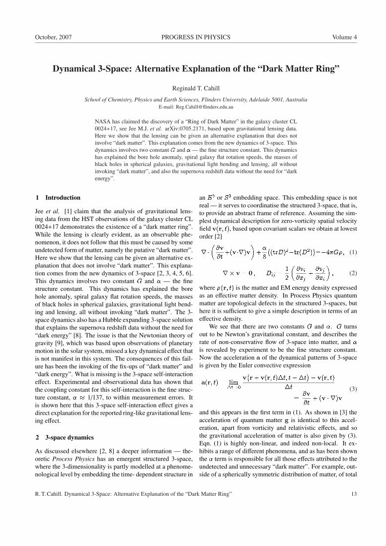
Fig. 1: Data shows the non-Keplerian rotation-speed curve vO forthe spiral galaxy NGC 3198 in km/s plotted against radius in kpc/h.Lower curve is the rotation curve from the Newtonian theory for anexponential disk, which decreases asymptotically like 1=
pr. The
upper curve shows the asymptotic form from (11), with the decreasedetermined by the small value of �. This asymptotic form is causedby the primordial black holes at the centres of spiral galaxies, andwhich play a critical role in their formation. The spiral structure iscaused by the rapid in-fall towards these primordial black holes.
parameter class of analytic solutions
v(r) = � rK
1r
+1Rs
�Rsr
��2!1=2
(9)
where K and Rs are arbitrary constants in the � = 0 region,but whose values are determined by matching to the solu-tion in the matter region. Here Rs characterises the lengthscale of the non-perturbative part of this expression, and Kdepends on �, G and details of the matter distribution. From(5) and (9) we obtain a replacement for the Newtonian “in-verse square law”
g(r) = � rK2
2
1r2 +
�2rRs
�Rsr
��2!: (10)
The 1st term, 1=r2, is the Newtonian part. The 2nd termis caused by a “black hole” phenomenon that (1) exhibits.This manifests in different ways, from minimal supermassiveblack holes, as seen in spherical star systems, from globularclusters to spherical galaxies for which the black hole mass ispredicted to be MBH = �M=2, as confirmed by the observa-tional datas [2, 4, 5, 6, 7], to primordial supermassive blackholes as seen in spiral galaxies as described by (9); here thematter spiral is caused by matter in-falling towards the pri-mordial black hole.
The spatial-inflow phenomenon in (9) is completely dif-ferent from the putative “black holes” of General Relativity— the new “black holes” have an essentially 1=r force law,up to O(�) corrections, rather than the usual Newtonain and
14 R. T. Cahill. Dynamical 3-Space: Alternative Explanation of the “Dark Matter Ring”
October, 2007 PROGRESS IN PHYSICS Volume 4
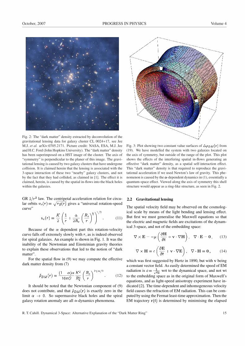
Fig. 2: The “dark matter” density extracted by deconvolution of thegravitational lensing data for galaxy cluster CL 0024+17, see JeeM.J. et al. arXiv:0705.2171. Picture credit: NASA, ESA, M.J. Jeeand H.C. Ford (John Hopkins University). The “dark matter” densityhas been superimposed on a HST image of the cluster. The axis of“symmetry” is perpendicular to the planer of this image. The gravi-tational lensing is caused by two galaxy clusters that have undergonecollision. It is claimed herein that the lensing is associated with the3-space interaction of these two “nearby” galaxy clusters, and notby the fact that they had collided, as claimed in [1]. The effect it isclaimed, herein, is caused by the spatial in-flows into the black holeswithin the galaxies.
GR 1=r2 law. The centripetal acceleration relation for circu-lar orbits v�(r) =
prg(r) gives a “universal rotation-speed
curve”
v�(r) =K2
1r
+�
2Rs
�Rsr
��2!1=2
: (11)
Because of the � dependent part this rotation-velocitycurve falls off extremely slowly with r, as is indeed observedfor spiral galaxies. An example is shown in Fig. 1. It was theinability of the Newtonian and Einsteinian gravity theoriesto explain these observations that led to the notion of “darkmatter”.
For the spatial flow in (9) we may compute the effectivedark matter density from (7)
~�DM (r) =(1� �)�
16�GK2
R3s
�Rsr
�2+�=2
: (12)
It should be noted that the Newtonian component of (9)does not contribute, and that ~�DM (r) is exactly zero in thelimit � ! 0. So supermassive black holes and the spiralgalaxy rotation anomaly are all �-dynamics phenomena.
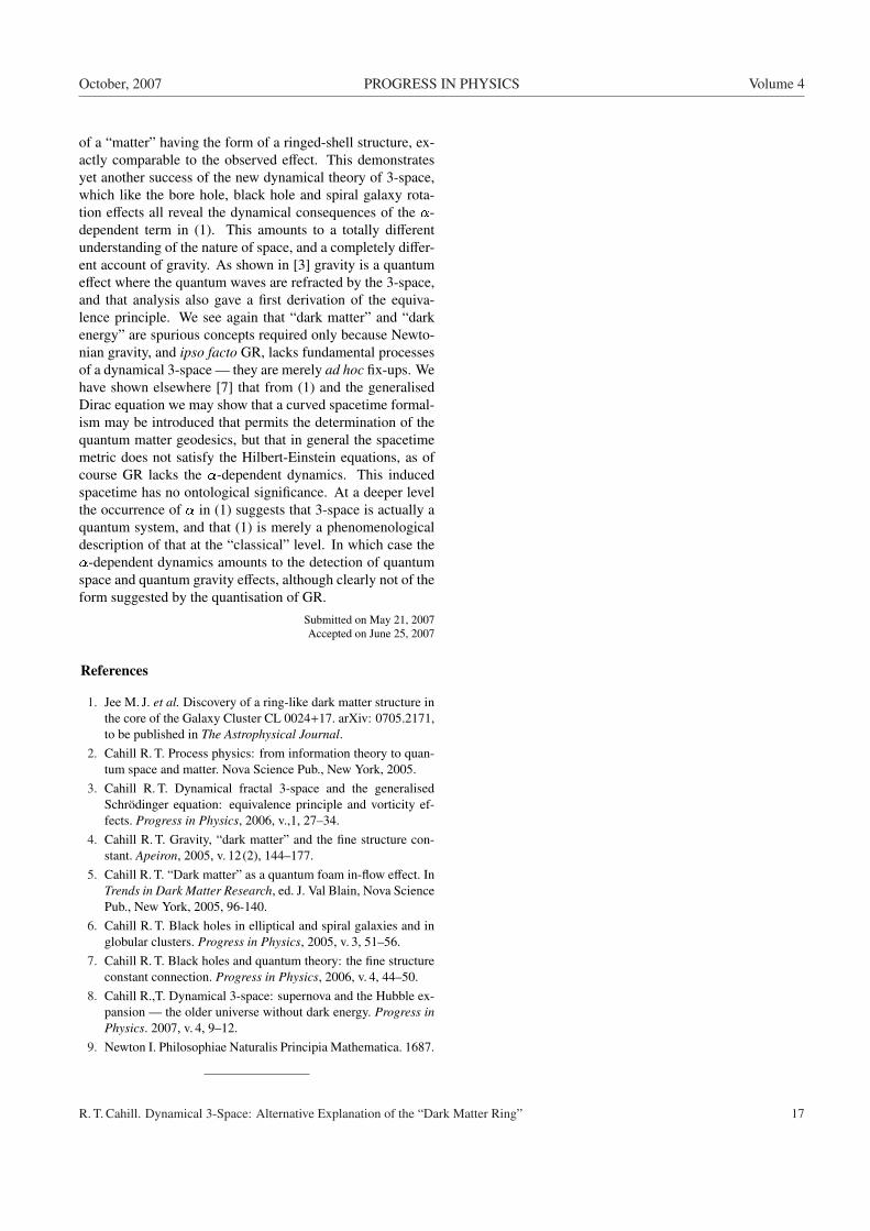
Fig. 3: Plot showing two constant value surfaces of ��DM (r) from(19). We have modelled the system with two galaxies located onthe axis of symmetry, but outside of the range of the plot. This plotshows the effects of the interfering spatial in-flows generating aneffective “dark matter” density, as a spatial self-interaction effect.This “dark matter” density is that required to reproduce the gravi-tational acceleration if we used Newton’s law of gravity. This phe-nomenon is caused by the�-dependent dynamics in (1), essentially aquantum-space effect. Viewed along the axis of symmetry this shellstructure would appear as a ring-like structure, as seen in Fig. 2.
2.2 Gravitational lensing
The spatial velocity field may be observed on the cosmolog-ical scale by means of the light bending and lensing effect.But first we must generalise the Maxwell equations so thatthe electric and magnetic fields are excitations of the dynam-ical 3-space, and not of the embedding space:
r�E = ���@H@t
+ v � rH�; r �E = 0 ; (13)
r�H = ��@E@t
+ v � rE�; r �H = 0 ; (14)
which was first suggested by Hertz in 1890, but with v beinga constant vector field. As easily determined the speed of EMradiation is c= 1p�� wrt to the dynamical space, and not wtto the embedding space as in the original form of Maxwell’sequations, and as light-speed anisotropy experiment have in-dicated [2]. The time-dependent and inhomogeneous velocityfield causes the refraction of EM radiation. This can be com-puted by using the Fermat least-time approximation. Then theEM trajectory r(t) is determined by minimising the elapsed
R. T. Cahill. Dynamical 3-Space: Alternative Explanation of the “Dark Matter Ring” 15

Volume 4 PROGRESS IN PHYSICS October, 2007
Fig. 4: Plot of ��DM (r) from (19) in a radial direction from a mid-point on the axis joining the two galaxies.
Fig. 5: Plot of ��DM (r) from (19) in the plane containing the twogalaxies. The two galaxies are located at +10 and -10, i.e above andbelow the vertical in this contour plot. This plot shows the effects ofthe interfering in-flows.
travel time:
� =Z sf
si
ds��drds
��jc vR(s) + v
�r(s); t(s)
�j (15)
vR =�drdt� v(r; t)
�(16)
by varying both r(s) and t(s), finally giving r(t). Here s isa path parameter, and vR is a 3-space tangent vector for thepath. As an example, the in-flow in (4), which is applicableto light bending by the sun, gives the angle of deflection
� = 2v2
c2=
4GM(1 + �2 + : : :)
c2d+ : : : (17)
where v is the in-flow speed at distance d and d is the impactparameter. This agrees with the GR result except for the �
correction. Hence the observed deflection of 8.4�10�6 radi-ans is actually a measure of the in-flow speed at the sun’s sur-face, and that gives v= 615 km/s. These generalised Maxwellequations also predict gravitational lensing produced by thelarge in-flows from (9) associated with the new “black holes”in galaxies. So again this effect permits the direct observationof the these black hole effects with their non inverse-square-law accelerations.
3 Galaxy Cluster lensing
It is straightforward to analyse the gravitational lensing pre-dicted by a galaxy cluster, with the data from CL 0024+17of particular interest. However rather than compute the ac-tual lensing images, we shall compute the “dark matter” ef-fective density from (7), and compare that with the putative“dark matter” density extracted from the actual lensing datain [1]. To that end we need to solve (1) for two reasonablyclose galaxies, located at positions R and �R. Here we lookfor a perturbative modification of the 3-space in-flows whenthe two galaxies are nearby. We take the velocity field in 1stapproximation to be the superposition
v(r) � v(r�R) + v(r + R) ; (18)
where the RHS v’s are from (9).Substituting this in (1) will then generate an improved
solution, keeping in mind that (1) is non-linear, and so thissuperposition cannot be exact. Indeed it is the non-linearityeffect which it is claimed herein is responsible for the ring-like structure reported in [1]. Substituting (18) in (7) we maycompute the change in the effective “dark matter” densitycaused by the two galaxies interfering with the in-flow intoeach separately, i.e.
��DM (r) = �DM (r)� ~�DM (r�R)� ~�DM (r + R) (19)
~�DM (r�R) are the the effective “dark matter” densities forone isolated galaxy in (12). Several graphical representationsof ��DM (r) are given in Figs. 3, 4 and 5. We seen thatviewed along the line of the two galaxies the change in theeffective “dark matter” density has the form of a ring, in par-ticular one should compare the predicted effective “dark mat-ter” density in Fig. 3 with that found by deconvoluting thegravitaitaional lensing data shown in shown Fig. 2.
4 Conclusions
We have shown that the dynamical 3-space theory gives a di-rect account of the observed gravitational lensing caused bytwo galaxy clusters, which had previously collided, but thatthe ring-like structure is not related to that collision, contraryto the claims in [1]. The distinctive lensing effect is causedby interference between the two spatial in-flows, resulting inEM refraction which appears to be caused by the presence
16 R. T. Cahill. Dynamical 3-Space: Alternative Explanation of the “Dark Matter Ring”
October, 2007 PROGRESS IN PHYSICS Volume 4
of a “matter” having the form of a ringed-shell structure, ex-actly comparable to the observed effect. This demonstratesyet another success of the new dynamical theory of 3-space,which like the bore hole, black hole and spiral galaxy rota-tion effects all reveal the dynamical consequences of the �-dependent term in (1). This amounts to a totally differentunderstanding of the nature of space, and a completely differ-ent account of gravity. As shown in [3] gravity is a quantumeffect where the quantum waves are refracted by the 3-space,and that analysis also gave a first derivation of the equiva-lence principle. We see again that “dark matter” and “darkenergy” are spurious concepts required only because Newto-nian gravity, and ipso facto GR, lacks fundamental processesof a dynamical 3-space — they are merely ad hoc fix-ups. Wehave shown elsewhere [7] that from (1) and the generalisedDirac equation we may show that a curved spacetime formal-ism may be introduced that permits the determination of thequantum matter geodesics, but that in general the spacetimemetric does not satisfy the Hilbert-Einstein equations, as ofcourse GR lacks the �-dependent dynamics. This inducedspacetime has no ontological significance. At a deeper levelthe occurrence of � in (1) suggests that 3-space is actually aquantum system, and that (1) is merely a phenomenologicaldescription of that at the “classical” level. In which case the�-dependent dynamics amounts to the detection of quantumspace and quantum gravity effects, although clearly not of theform suggested by the quantisation of GR.
Submitted on May 21, 2007Accepted on June 25, 2007
References
1. Jee M. J. et al. Discovery of a ring-like dark matter structure inthe core of the Galaxy Cluster CL 0024+17. arXiv: 0705.2171,to be published in The Astrophysical Journal.
2. Cahill R. T. Process physics: from information theory to quan-tum space and matter. Nova Science Pub., New York, 2005.
3. Cahill R. T. Dynamical fractal 3-space and the generalisedSchrodinger equation: equivalence principle and vorticity ef-fects. Progress in Physics, 2006, v.,1, 27–34.
4. Cahill R. T. Gravity, “dark matter” and the fine structure con-stant. Apeiron, 2005, v. 12(2), 144–177.
5. Cahill R. T. “Dark matter” as a quantum foam in-flow effect. InTrends in Dark Matter Research, ed. J. Val Blain, Nova SciencePub., New York, 2005, 96-140.
6. Cahill R. T. Black holes in elliptical and spiral galaxies and inglobular clusters. Progress in Physics, 2005, v. 3, 51–56.
7. Cahill R. T. Black holes and quantum theory: the fine structureconstant connection. Progress in Physics, 2006, v. 4, 44–50.
8. Cahill R.,T. Dynamical 3-space: supernova and the Hubble ex-pansion — the older universe without dark energy. Progress inPhysics. 2007, v. 4, 9–12.
9. Newton I. Philosophiae Naturalis Principia Mathematica. 1687.
R. T. Cahill. Dynamical 3-Space: Alternative Explanation of the “Dark Matter Ring” 17
Volume 4 PROGRESS IN PHYSICS October, 2007
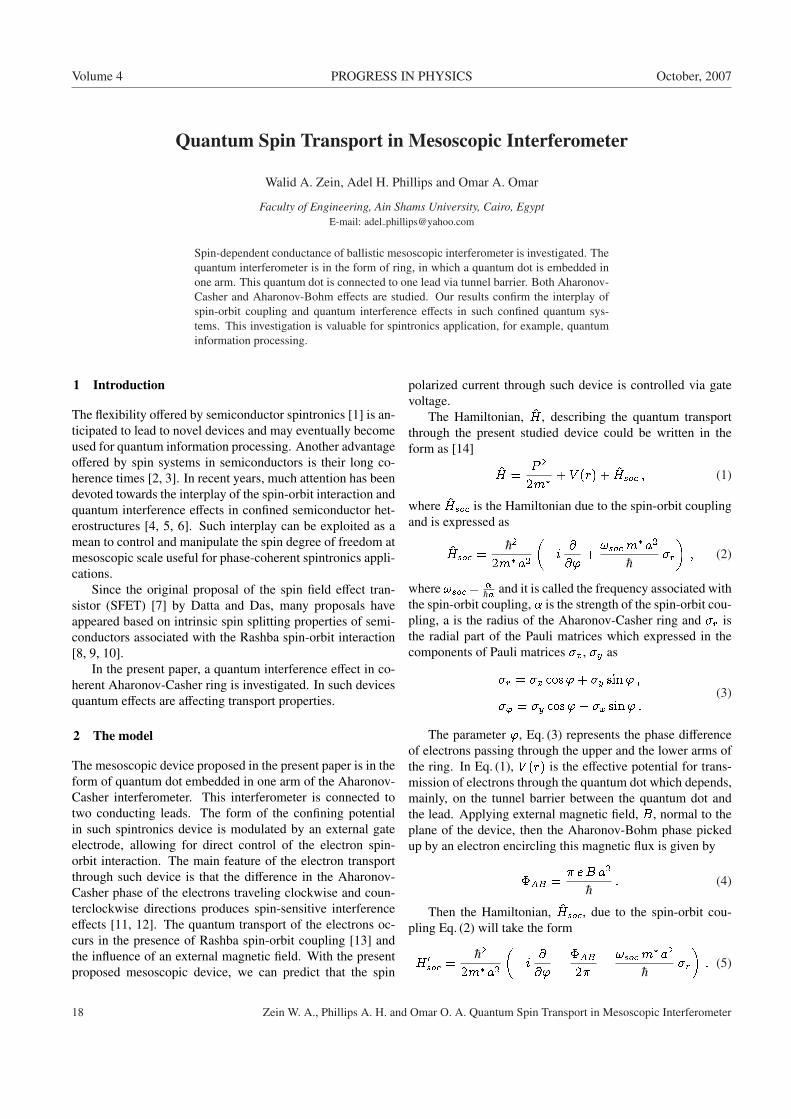
Quantum Spin Transport in Mesoscopic Interferometer
Walid A. Zein, Adel H. Phillips and Omar A. Omar
Faculty of Engineering, Ain Shams University, Cairo, EgyptE-mail: adel [email protected]
Spin-dependent conductance of ballistic mesoscopic interferometer is investigated. Thequantum interferometer is in the form of ring, in which a quantum dot is embedded inone arm. This quantum dot is connected to one lead via tunnel barrier. Both Aharonov-Casher and Aharonov-Bohm effects are studied. Our results confirm the interplay ofspin-orbit coupling and quantum interference effects in such confined quantum sys-tems. This investigation is valuable for spintronics application, for example, quantuminformation processing.
1 Introduction
The flexibility offered by semiconductor spintronics [1] is an-ticipated to lead to novel devices and may eventually becomeused for quantum information processing. Another advantageoffered by spin systems in semiconductors is their long co-herence times [2, 3]. In recent years, much attention has beendevoted towards the interplay of the spin-orbit interaction andquantum interference effects in confined semiconductor het-erostructures [4, 5, 6]. Such interplay can be exploited as amean to control and manipulate the spin degree of freedom atmesoscopic scale useful for phase-coherent spintronics appli-cations.
Since the original proposal of the spin field effect tran-sistor (SFET) [7] by Datta and Das, many proposals haveappeared based on intrinsic spin splitting properties of semi-conductors associated with the Rashba spin-orbit interaction[8, 9, 10].
In the present paper, a quantum interference effect in co-herent Aharonov-Casher ring is investigated. In such devicesquantum effects are affecting transport properties.
2 The model
The mesoscopic device proposed in the present paper is in theform of quantum dot embedded in one arm of the Aharonov-Casher interferometer. This interferometer is connected totwo conducting leads. The form of the confining potentialin such spintronics device is modulated by an external gateelectrode, allowing for direct control of the electron spin-orbit interaction. The main feature of the electron transportthrough such device is that the difference in the Aharonov-Casher phase of the electrons traveling clockwise and coun-terclockwise directions produces spin-sensitive interferenceeffects [11, 12]. The quantum transport of the electrons oc-curs in the presence of Rashba spin-orbit coupling [13] andthe influence of an external magnetic field. With the presentproposed mesoscopic device, we can predict that the spin
polarized current through such device is controlled via gatevoltage.
The Hamiltonian, H, describing the quantum transportthrough the present studied device could be written in theform as [14]
H =P 2
2m� + V (r) + Hsoc ; (1)
where Hsoc is the Hamiltonian due to the spin-orbit couplingand is expressed as
Hsoc =~2
2m�a2
��i @
@'+!socm�a2
~�r�; (2)
where !soc = �~a and it is called the frequency associated with
the spin-orbit coupling, � is the strength of the spin-orbit cou-pling, a is the radius of the Aharonov-Casher ring and �r isthe radial part of the Pauli matrices which expressed in thecomponents of Pauli matrices �x, �y as
�r = �x cos'+ �y sin' ;
�' = �y cos'� �x sin' :(3)
The parameter ', Eq. (3) represents the phase differenceof electrons passing through the upper and the lower arms ofthe ring. In Eq. (1), V (r) is the effective potential for trans-mission of electrons through the quantum dot which depends,mainly, on the tunnel barrier between the quantum dot andthe lead. Applying external magnetic field, B, normal to theplane of the device, then the Aharonov-Bohm phase pickedup by an electron encircling this magnetic flux is given by
�AB =� eB a2
~: (4)
Then the Hamiltonian, Hsoc, due to the spin-orbit cou-pling Eq. (2) will take the form
H 0soc =~2
2m�a2
��i @
@'� �AB
2�� !socm�a2
~�r�: (5)
18 Zein W. A., Phillips A. H. and Omar O. A. Quantum Spin Transport in Mesoscopic Interferometer

October, 2007 PROGRESS IN PHYSICS Volume 4
Now in order to study the transport properties of the pre-sent quantum system, we have to solve Schrodinger equationand finding the eigenfunctions for this system as follows
H = E : (6)
The solution of Eq. (6) consists of four eigenfunctions[14], where L(x) is the eigenfunction for transmissionthrough the left lead, R(x)-for the right lead, up(�)-forthe upper arm of the ring and low(�)-for the lower arm ofthe ring. Their forms will be as
L(x) =X�
�Aeikx +B e�ikx
���(�) ;
x 2 [�1; 0] ;(7a)
R(x) =X�
hC eikx
0+ De�ikx0
i��(0) ;
x 2 [0;1] ;
(7b)
up(') =X�;�
F� ein0��' ��(') ;
' 2 [0; �] ;
(7c)
low(') =X�;�
G� ein��' ��(') ;
' 2 [�; 2�] :
(7d)
The mutually orthogonal spinors �n(') are expressed in
terms of the eigenvectors�
10
�,�
01
�of the Pauli matrix �z as
�(1)n (') =
cos �2
ei' sin �2
!; (7)
�(2)n (') =
sin �
2
�ei' cos �2
!; (8)
where the angle � [15] is given by
� = 2 tan�1 � p2 + !2soc
!soc(9)
in which is given by
=~
2m�a2 : (10)
The parameters n0�� and n�� are expressed respectively as
n0�� = �k0a� '+�AB2�
+��AC2�
; (11)
n�� = �ka� '+�AB2�
+��AC2�
; (12)
where �=�1 corresponding to the spin up and spin downof transmitted electrons, �AB is given by Eq. (4). The term�AC represents the Aharonov-Casher phase and is given by
�(�)AC = ��
�1 +
(�1)�(!2soc + 2)1=2
�: (13)
The wave numbers k0, k are given respectively by
k0 =r
2m�E~2 ; (14)
k =
s2m�~2
�Vd + e Vg +
N2e2
2C+ EF � E
�; (15)
where Vd is the barrier height, Vg is the gate voltage, N is thenumber of electrons entering the quantum dot, C is the totalcapacitance of the quantum dot, m� is the effective mass ofelectrons with energy, E, and charge, e, and EF is the Fermienergy.
The conductance, G, for the present investigated devicewill be calculated using landauer formula [16] as
G =2e2 sin'
h
X�=1;2
ZdE��@fFD
@E
�j��(E)j2 ; (16)
where fFD is the Fermi-Dirac distribution is function andj��(E)j2 is tunneling probability. This tunneling probabilitycould be obtained by applying the Griffith boundary condi-tions [15, 17, 18], which states that the eigenfunctions(Eqs. 7a, 7b, 7c, 7d) are continuous and that the current den-sity is conserved at each intersection. Then the expression for��(E) is given by
��(E) =
=8i cos �AB+�(�)
AC2 sin(�ka)
4 cos(2�k0a)+4 cos��AB+�(�)
AC
�+4i sin(2�k0a)
: (17)
3 Results and discussion
In order to investigate the quantum spin transport character-istics through the present device, we solve Eqs. (17, 18) nu-merically. We use the heterostructures as InGaAs/InAlAs.
We calculate the conductance, G, at different both mag-netic field and the !soc which depends on the Rashba spin-orbit coupling strength. The main features of our obtainedresults are:
1. Figs. 1 and Fig. 2 show the dependence of the conduc-tance on the magnetic field, B, for small and large val-ues of B at different !soc.
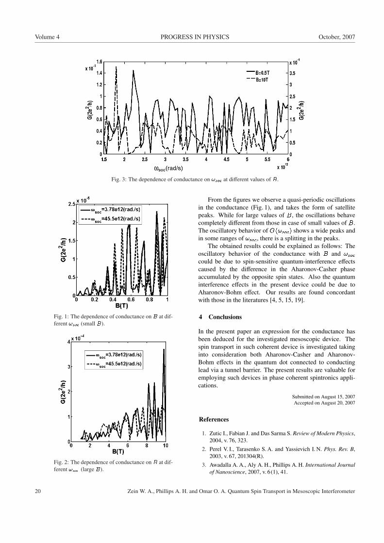
2. Fig. 3 shows the dependence of the conductance on theparameter !soc at different values of B.
Zein W. A., Phillips A. H. and Omar O. A. Quantum Spin Transport in Mesoscopic Interferometer 19
Volume 4 PROGRESS IN PHYSICS October, 2007
Fig. 3: The dependence of conductance on !soc at different values of B.
Fig. 1: The dependence of conductance on B at dif-ferent !soc (small B).
Fig. 2: The dependence of conductance on B at dif-ferent !soc (large B).
From the figures we observe a quasi-periodic oscillationsin the conductance (Fig. 1), and takes the form of satellitepeaks. While for large values of B, the oscillations behavecompletely different from those in case of small values of B.The oscillatory behavior of G(!soc) shows a wide peaks andin some ranges of !soc, there is a splitting in the peaks.
The obtained results could be explained as follows: Theoscillatory behavior of the conductance with B and !soccould be due to spin-sensitive quantum-interference effectscaused by the difference in the Aharonov-Casher phaseaccumulated by the opposite spin states. Also the quantuminterference effects in the present device could be due toAharonov-Bohm effect. Our results are found concordantwith those in the literatures [4, 5, 15, 19].
4 Conclusions
In the present paper an expression for the conductance hasbeen deduced for the investigated mesoscopic device. Thespin transport in such coherent device is investigated takinginto consideration both Aharonov-Casher and Aharonov-Bohm effects in the quantum dot connected to conductinglead via a tunnel barrier. The present results are valuable foremploying such devices in phase coherent spintronics appli-cations.
Submitted on August 15, 2007Accepted on August 20, 2007
References
1. Zutic I., Fabian J. and Das Sarma S. Review of Modern Physics,2004, v. 76, 323.
2. Perel V. I., Tarasenko S. A. and Yassievich I. N. Phys. Rev. B,2003, v. 67, 201304(R).
3. Awadalla A. A., Aly A. H., Phillips A. H. International Journalof Nanoscience, 2007, v. 6(1), 41.
20 Zein W. A., Phillips A. H. and Omar O. A. Quantum Spin Transport in Mesoscopic Interferometer
October, 2007 PROGRESS IN PHYSICS Volume 4
4. Nitta J., Meijer F. E., and Takayanagi H. Appl. Phys. Lett., 1999,v. 75, 695.
5. Molnar B., Vasilopoulos P., and Peeters F. M. Appl. Phys. Lett.,2004, v. 85, 612.
6. Rashba E. I. Phys. Rev. B, 2000, v. 62, R16267.
7. Datta S. and Das B. Appl. Phys. Lett., 1990, v. 56, 665.
8. Meijer P. E., Morpurgo A. F. and Klapwijk T. M. Phys. Rev. B,2002, v. 66, 033107.
9. Grundler D. Phys. Rev. Lett., 2000, v. 84, 6074.
10. Kiselev A. A. and Kim K. W. J. Appl. Phys., 2003, v. 94, 4001.
11. Aharonov Y. and Casher A. Phys. Rev. Lett., 1984, v. 53, 319.
12. Yau J. B., De Pootere E. P., and Shayegan M. Phys. Rev. Lett.,2003, v. 88, 146801.
13. Rashba E. I. Sov. Phys. Solid State, 1960, v. 2, 1109.
14. Hentschel M., Schomerus H., Frustaglia D. and Richter K.Phys. Rev. B, 2004, v. 69, 155326.
15. Molnar B., Peeters F. M. and Vasilopoulos P. Phys. Rev. B,2004, v. 69, 155335.
16. Datta S. Electronic transport in mesoscopis systems. Cam-bridge Unversity Press, Cambridge, 1997.
17. Griffith S. Trans. Faraday Soc., 1953, v. 49, 345.
18. Xia J. B. Phys. Rev. B, 1992, v. 45, 3593.
19. Citro R., Romeo F. and Marinaro M. Phys. Rev. B, 2006, v. 74,115329.
Zein W. A., Phillips A. H. and Omar O. A. Quantum Spin Transport in Mesoscopic Interferometer 21

Volume 4 PROGRESS IN PHYSICS October, 2007
Some Remarks on Ricci Flow and the Quantum Potential
Robert Carroll
University of Illinois, Urbana, IL 61801, USAE-mail: [email protected]
We indicate some formulas connecting Ricci flow and Perelman entropy to Fisher in-formation, differential entropy, and the quantum potential. There is a known relationinvolving the Schroedinger equation in a Weyl space where the Weyl-Ricci curvature isproportional to the quantum potential. The quantum potential in turn is related to Fisherinformation which is given via the Perelman entropy functional arising from a differ-ential entropy under Ricci flow. These relations are written out and seem to suggestconnections between quantum mechanics and Ricci flow.
1 Formulas involving Ricci flow
Certain aspects of Perelman’s work on the Poincare conjec-ture have applications in physics and we want to suggest afew formulas in this direction; a fuller exposition will appearin a book in preparation [8]. We go first to [13, 24–28, 33, 39]and simply write down a few formulas from [28, 39] here withminimal explanation. Thus one has Perelman’s functional( _R is the Riemannian Ricci curvature)
F =ZM
( _R+ jrf j2) exp(�f)dV (1.1)
and a so-called Nash entropy (1A) N(u) =RM u log(u)dV
where u = exp (�f). One considers Ricci flows with�g� @tg=h and for (1B) ��u=�@tu��u+ _Ru= 0(or equivalently @tf + �f � jrf j2 + _R= 0) it follows thatRM exp(�f)dV =1 is preserved and @tN=F. Note the Ricci
flow equation is @t g=�2Ric. Extremizing F via �F�� @tF= 0 involves Ric+Hess(f) = 0 or Rij +rirjf = 0and one knows also that
@tN =ZM
(jrf j2 + _R) exp(�f)dV = F ;
@tF = 2ZMjRic+Hess(f)j2 exp(�f)dV:
(1.2)
2 The Schrodinger equation and WDW
Now referring to [3–5, 7–12, 15, 16, 18–23, 29–32, 35–38, 40]for details we note first the important observation in [39] thatF is in fact a Fisher information functional. Fisher informa-tion has come up repeatedly in studies of the Schrodingerequation (SE) and the Wheeler-deWitt equation (WDW) andis connected to a differential entropy correspondingto theNash entropy above (cf. [4, 7, 18, 19]). The basic ideasinvolve (using 1-D for simplicity) a quantum potential Q suchthat
RM P Qdx �F arising from a wave function =
=R exp(iS=~) where Q=�(~2=2m)(�R=R) and P � j j2
is a probability density. In a WDW context for example onecan develop a framework
Q = cP�1=2 @(GP 1=2);ZQP = c
ZP 1=2@(GP 1=2)Dhdx !
! � cZ@P 1=2G@P 1=2Dhdx
9>>>>>>=>>>>>>;(2.1)
where G is an expression involving the deWitt metricGijk`(h). In a more simple minded context consider a SE in1-D i~@t =�(~2=2m)@2
x +V where =R exp(iS=~)leads to the equations
St +1
2mS2x +Q+ V = 0;
@tR2 +1m
(R2Sx)x = 0 : Q = � ~2
2mRxxR
:
9>>=>>; (2.2)
In terms of the exact uncertainty principle of Hall andReginatto (see [21, 23, 34] and cf. also [4, 6, 7, 31, 32])the quantum Hamiltonian has a Fisher information termcRdx(rP � rP=2mP ) added to the classical Hamiltonian
(where P =R2� j j2) and a simple calculation givesZPQd3x � � ~2
8m
Z �2�P � 1
PjrP j2
�d3x =
=~2
8m
Z1PjrP j2 d3x :
(2.3)
In the situation of (2.1) the analogues to Section 1 involve(@ � @x)
P � e�f ; P 0 � Px � �f 0e�f ;
Q� ef=2@(G@e�f=2); PQ� e�f=2@(G@e�f=2);ZPQ! �
Z@e�f=2G@e�f=2 � �
Z@P 1=2G@P 1=2:
9>>>>>>=>>>>>>;(2.4)
22 R. Carroll. Some Remarks on Ricci Flow and the Quantum Potential

October, 2007 PROGRESS IN PHYSICS Volume 4
In the context of the SE in Weyl space developed in [1, 2,4, 7, 10, 11, 12, 35, 36, 40] one has a situation j j2�R2��P � � = �=pg with a Weyl vector ~� =�r log(�) and aquantum potential
Q � � ~2
16m
�_R+
8p�
1pg @i�p
g gik@kp���
=
= � ~2
16m
�_R+
8p�
�p�� (2.5)
(recall divgrad(U) = �U= (1=pg)@m(pggmn@nU). Herethe Weyl-Ricci curvature is (2A) R = _R+Rw where
Rw = 2 j~�j2 � 4r � ~� = 8�p�p�
(2.6)
and Q = �(~2=16m)R. Note that
�r � ~� � �� log(�) � ����
+jr�j2�2 (2.7)
and for exp(�f) = � = uZ�r � ~� dV =
Z ����+
jr�j2�
�dV (2.8)
with the first term in the last integral vanishing and the secondproviding Fisher information again. Comparing with Sec-tion 1 we have analogues (2B) G� (R+ j~�j2) with ~�==�r log(�)�rf to go with (2.4). Clearly � is basically aprobability concept with
R� dV = 1 and Quantum Mechan-
ics (QM) (or rather perhaps Bohmian mechanics) seems toenter the picture through the second equation in (2.2), namely(2C) @t � + (1=m) div(�rS) = 0 with p = mv =rS,which must be reconciled with (1B) (i.e. (1=m) div(urS) == �u� _Ru). In any event the termG= _R+ j~�j2 can be writ-ten as (2D) _R+Rw + (j~�j2�Rw) =�Q+ (4r � ~�� j~�j2)which leads to (2E) F�� RM QP dV +�
R j~�j2PdV put-ting Q directly into the picture and suggesting some sort ofquantum mechanical connection.
REMARK 2.1. We mention also that Q appears in a fascinat-ing geometrical role in the relativistic Bohmian format fol-lowing [3, 15, 37, 38] (cf. also [4, 7] for survey material).Thus e.g. one can define a quantum mass field via
M2 = m2 exp(Q) � m2(1 +Q);
Q � �~2
c2m2�(p�)p� � �
6Rw
(2.9)
where � refers to an appropriate mass density andM is in factthe Dirac field � in a Weyl-Dirac formulation of Bohmianquantum gravity. Further one can change the 4-D Lorentzianmetric via a conformal factor 2 =M2=m2 in the form ~g�� == 2g�� and this suggests possible interest in Ricci flows etc.
in conformal Lorentzian spaces (cf. here also [14]). We referto [3, 15] for another fascinating form of the quantum poten-tial as a mass generating term and intrinsic self energy. �
NOTE. Publication information for items below listed byarchive numbers can often be found on the net listing. �
Submitted on June 27, 2007Accepted on June 29, 2007
References
1. Audretsch J. Phys. Rev. D, 1983, v. 27, 2872–2884.
2. Audretsch J., Gahler F. and Straumann N., Comm. Math. Phys.,1984, v. 95, 41–51.
3. Bertoldi G., Faraggi A. and Matone M. Class. Quant. Grav.,2000, v. 17, 3965; arXiv: hep-th/9909201.
4. Carroll R. Fluctuations, information, gravity, and the quantumpotential. Springer, 2006.
5. Carroll R. arXiv: physics/0511076 and 0602036.
6. Carroll R. arXiv: gr-qc/0512146.
7. Carroll R. arXiv: math-ph/0701077.
8. Carroll R. On the quantum potential. (Book in preparation.)
9. Carroll R. Teor. Mat. Fizika, (to appear).
10. Carroll R. Found. Phys., 2005, v. 35, 131–154.
11. Castro C. Found. Phys., 1992, v. 22, 569–615; Found. Phys.Lett., 1991, v. 4, 81.
12. Castro C. and Mahecha J. Prog. Phys., 2006, v. 1, 38–45.
13. Chow B. and Knopf D. The Ricci flow: An introduction. Amer.Math. Soc., 2004.
14. Crowell L. Quantum fluctuations of spacetime. World Scien-tific, 2005.
15. Faraggi A. and Matone M. Inter. Jour. Mod. Phys. A, 2000,v. 15, 1869–2017; arXiv: hep-th/9809127.
16. Frieden B. Physics from Fisher information. Cambridge Univ.Press, 1998.
17. Fujii Y. and Maeda K. The scalar tensor theory of gravitation.Cambridge Univ. Press, 2003.
18. Garbaczewski P. arXiv: cond-mat/0211362 and 0301044.
19. Garbaczdwski P. arXiv: quant-ph/0408192; Jour. Stat. Phys.,2006, v. 123, 315–355.
20. Garbaczewski P. arXiv: cond-mat/0604538; quant-ph/0612151.
21. Hall M. arXiv: gr-qc/0408098.
22. Hall M., Kumar K. and Reginatto M. arXiv: quant-ph/0103041.
23. Hall M., Kumar K. and Reginatto M. Jour. Phys. A, 2003, v. 36,9779–9794; arXiv: hep-th/0206235 and 0307259.
24. Jost J. Riemannian geometry and geometric analysis. Springer,2002.
25. Kholodenko A. arXiv: gr-qc/0010064; hep-th/0701084.
26. Kholodenko A. and Ballard E. arXiv: gr-qc/0410029.
27. Kholodenko A. and Freed K. Jour. Chem. Phys., 1984, v. 80,900–924.
R. Carroll. Some Remarks on Ricci Flow and the Quantum Potential 23

Volume 4 PROGRESS IN PHYSICS October, 2007
28. Muller R. Differential Harnack inequalities and the Ricci flow.Eur. Math. Soc. Pub. House, 2006.
29. Nikolic H. Euro. Phys. Jour. C, 2005, v. 421, 365–374; arXiv:hep-th/0407228; gr-qc/9909035 and 0111029; hep-th/0202204and 0601027.
30. Nikolic H. arXiv: gr-qc/0312063; hep-th/0501046; quant-ph/0603207 and 0512065.
31. Parwani R. arXiv: quant-ph/0408185 and 0412192; hep-th/0401190.
32. Parwani R. arXiv: quant-ph/0506005 and 0508125.
33. Perelman G. arXiv: math.DG/0211159, 0303109, and0307245.
34. Reginatto M. arXiv: quant-ph/9909065.
35. Santamato E. Phys. Rev. D, 1984, v. 29, 216–222.
36. Santamato E. Phys. Rev. D, 1985, v. 32, 2615–26221; Jour.Math. Phys., 1984, v. 25, 2477–2480.
37. Shojai F. and Shojai A. arXiv: gr-qc/0306099.
38. Shojai F. and Shojai A. arXiv: gr-qc/0404102.
39. Topping P. Lectures on the Ricci flow. Cambridge Univ. Press,2006.
40. Wheeler J. Phys. Rev. D, 1990, v. 41, 431–441; 1991, v. 44,1769–1773.
24 R. Carroll. Some Remarks on Ricci Flow and the Quantum Potential
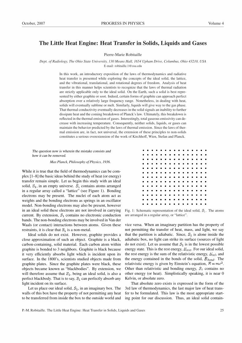
October, 2007 PROGRESS IN PHYSICS Volume 4
The Little Heat Engine: Heat Transfer in Solids, Liquids and Gases
Pierre-Marie Robitaille
Dept. of Radiology, The Ohio State University, 130 Means Hall, 1654 Upham Drive, Columbus, Ohio 43210, USAE-mail: [email protected]
In this work, an introductory exposition of the laws of thermodynamics and radiativeheat transfer is presented while exploring the concepts of the ideal solid, the lattice,and the vibrational, translational, and rotational degrees of freedom. Analysis of heattransfer in this manner helps scientists to recognize that the laws of thermal radiationare strictly applicable only to the ideal solid. On the Earth, such a solid is best repre-sented by either graphite or soot. Indeed, certain forms of graphite can approach perfectabsorption over a relatively large frequency range. Nonetheless, in dealing with heat,solids will eventually sublime or melt. Similarly, liquids will give way to the gas phase.That thermal conductivity eventually decreases in the solid signals an inability to furtherdissipate heat and the coming breakdown of Planck’s law. Ultimately, this breakdown isreflected in the thermal emission of gases. Interestingly, total gaseous emissivity can de-crease with increasing temperature. Consequently, neither solids, liquids, or gases canmaintain the behavior predicted by the laws of thermal emission. Since the laws of ther-mal emission are, in fact, not universal, the extension of these principles to non-solidsconstitutes a serious overextension of the work of Kirchhoff, Wien, Stefan and Planck.
The question now is wherein the mistake consists andhow it can be removed.
Max Planck, Philosophy of Physics, 1936.
While it is true that the field of thermodynamics can be com-plex [1–8] the basic ideas behind the study of heat (or energy)transfer remain simple. Let us begin this study with an idealsolid, S1, in an empty universe. S1 contains atoms arrangedin a regular array called a “lattice” (see Figure 1). Bondingelectrons may be present. The nuclei of each atom act asweights and the bonding electrons as springs in an oscillatormodel. Non-bonding electrons may also be present, howeverin an ideal solid these electrons are not involved in carryingcurrent. By extension, S1 contains no electronic conductionbands. The non-bonding electrons may be involved in Van derWaals (or contact) interactions between atoms. Given theserestraints, it is clear that S1 is a non-metal.
Ideal solids do not exist. However, graphite provides aclose approximation of such an object. Graphite is a black,carbon-containing, solid material. Each carbon atom withingraphite is bonded to 3 neighbors. Graphite is black becauseit very efficiently absorbs light which is incident upon itssurface. In the 1800’s, scientists studied objects made fromgraphite plates. Since the graphite plates were black, theseobjects became known as “blackbodies”. By extension, wewill therefore assume that S1, being an ideal solid, is also aperfect blackbody. That is to say, S1 can perfectly absorb anylight incident on its surface.
Let us place our ideal solid, S1, in an imaginary box. Thewalls of this box have the property of not permitting any heatto be transferred from inside the box to the outside world and
Fig. 1: Schematic representation of the ideal solid, S1. The atomsare arranged in a regular array, or “lattice”.
vice versa. When an imaginary partition has the property ofnot permitting the transfer of heat, mass, and light, we saythat the partition is adiabatic. Since, S1 is alone inside theadiabatic box, no light can strike its surface (sources of lightdo not exist). Let us assume that S1 is in the lowest possibleenergy state. This is the rest energy, Erest. For our ideal solid,the rest energy is the sum of the relativistic energy, Erel, andthe energy contained in the bonds of the solid, Ebond. Therelativistic energy is given by Einstein’s equation, E=mc2.Other than relativistic and bonding energy, S1 contains noother energy (or heat). Simplistically speaking, it is near 0Kelvin, or absolute zero.
That absolute zero exists is expressed in the form of the3rd law of thermodynamics, the last major law of heat trans-fer to be formulated. This law is the most appropriate start-ing point for our discussion. Thus, an ideal solid contain-
P.-M. Robitaille. The Little Heat Engine: Heat Transfer in Solids, Liquids and Gases 25
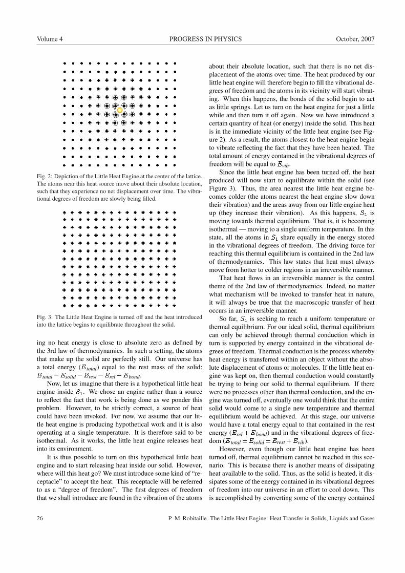
Volume 4 PROGRESS IN PHYSICS October, 2007
Fig. 2: Depiction of the Little Heat Engine at the center of the lattice.The atoms near this heat source move about their absolute location,such that they experience no net displacement over time. The vibra-tional degrees of freedom are slowly being filled.
Fig. 3: The Little Heat Engine is turned off and the heat introducedinto the lattice begins to equilibrate throughout the solid.
ing no heat energy is close to absolute zero as defined bythe 3rd law of thermodynamics. In such a setting, the atomsthat make up the solid are perfectly still. Our universe hasa total energy (E total) equal to the rest mass of the solid:E total =Esolid =Erest =Erel +Ebond.
Now, let us imagine that there is a hypothetical little heatengine inside S1. We chose an engine rather than a sourceto reflect the fact that work is being done as we ponder thisproblem. However, to be strictly correct, a source of heatcould have been invoked. For now, we assume that our lit-tle heat engine is producing hypothetical work and it is alsooperating at a single temperature. It is therefore said to beisothermal. As it works, the little heat engine releases heatinto its environment.
It is thus possible to turn on this hypothetical little heatengine and to start releasing heat inside our solid. However,where will this heat go? We must introduce some kind of “re-ceptacle” to accept the heat. This receptacle will be referredto as a “degree of freedom”. The first degrees of freedomthat we shall introduce are found in the vibration of the atoms
about their absolute location, such that there is no net dis-placement of the atoms over time. The heat produced by ourlittle heat engine will therefore begin to fill the vibrational de-grees of freedom and the atoms in its vicinity will start vibrat-ing. When this happens, the bonds of the solid begin to actas little springs. Let us turn on the heat engine for just a littlewhile and then turn it off again. Now we have introduced acertain quantity of heat (or energy) inside the solid. This heatis in the immediate vicinity of the little heat engine (see Fig-ure 2). As a result, the atoms closest to the heat engine beginto vibrate reflecting the fact that they have been heated. Thetotal amount of energy contained in the vibrational degrees offreedom will be equal to Evib.
Since the little heat engine has been turned off, the heatproduced will now start to equilibrate within the solid (seeFigure 3). Thus, the area nearest the little heat engine be-comes colder (the atoms nearest the heat engine slow downtheir vibration) and the areas away from our little engine heatup (they increase their vibration). As this happens, S1 ismoving towards thermal equilibrium. That is, it is becomingisothermal — moving to a single uniform temperature. In thisstate, all the atoms in S1 share equally in the energy storedin the vibrational degrees of freedom. The driving force forreaching this thermal equilibrium is contained in the 2nd lawof thermodynamics. This law states that heat must alwaysmove from hotter to colder regions in an irreversible manner.
That heat flows in an irreversible manner is the centraltheme of the 2nd law of thermodynamics. Indeed, no matterwhat mechanism will be invoked to transfer heat in nature,it will always be true that the macroscopic transfer of heatoccurs in an irreversible manner.
So far, S1 is seeking to reach a uniform temperature orthermal equilibrium. For our ideal solid, thermal equilibriumcan only be achieved through thermal conduction which inturn is supported by energy contained in the vibrational de-grees of freedom. Thermal conduction is the process wherebyheat energy is transferred within an object without the abso-lute displacement of atoms or molecules. If the little heat en-gine was kept on, then thermal conduction would constantlybe trying to bring our solid to thermal equilibrium. If therewere no processes other than thermal conduction, and the en-gine was turned off, eventually one would think that the entiresolid would come to a single new temperature and thermalequilibrium would be achieved. At this stage, our universewould have a total energy equal to that contained in the restenergy (Erel +Ebond) and in the vibrational degrees of free-dom (E total =Esolid =Erest +Evib).
However, even though our little heat engine has beenturned off, thermal equilibrium cannot be reached in this sce-nario. This is because there is another means of dissipatingheat available to the solid. Thus, as the solid is heated, it dis-sipates some of the energy contained in its vibrational degreesof freedom into our universe in an effort to cool down. Thisis accomplished by converting some of the energy contained
26 P.-M. Robitaille. The Little Heat Engine: Heat Transfer in Solids, Liquids and Gases
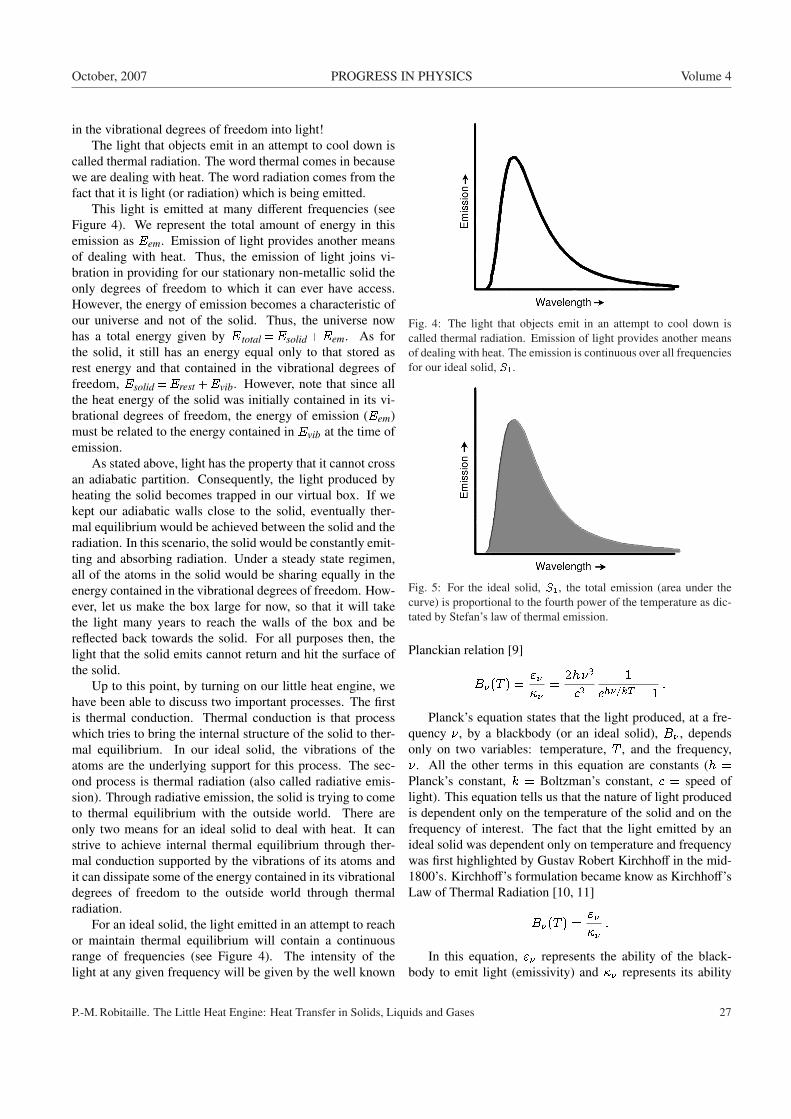
October, 2007 PROGRESS IN PHYSICS Volume 4
in the vibrational degrees of freedom into light!The light that objects emit in an attempt to cool down is
called thermal radiation. The word thermal comes in becausewe are dealing with heat. The word radiation comes from thefact that it is light (or radiation) which is being emitted.
This light is emitted at many different frequencies (seeFigure 4). We represent the total amount of energy in thisemission as Eem. Emission of light provides another meansof dealing with heat. Thus, the emission of light joins vi-bration in providing for our stationary non-metallic solid theonly degrees of freedom to which it can ever have access.However, the energy of emission becomes a characteristic ofour universe and not of the solid. Thus, the universe nowhas a total energy given by E total =Esolid +Eem. As forthe solid, it still has an energy equal only to that stored asrest energy and that contained in the vibrational degrees offreedom, Esolid =Erest +Evib. However, note that since allthe heat energy of the solid was initially contained in its vi-brational degrees of freedom, the energy of emission (Eem)must be related to the energy contained in Evib at the time ofemission.
As stated above, light has the property that it cannot crossan adiabatic partition. Consequently, the light produced byheating the solid becomes trapped in our virtual box. If wekept our adiabatic walls close to the solid, eventually ther-mal equilibrium would be achieved between the solid and theradiation. In this scenario, the solid would be constantly emit-ting and absorbing radiation. Under a steady state regimen,all of the atoms in the solid would be sharing equally in theenergy contained in the vibrational degrees of freedom. How-ever, let us make the box large for now, so that it will takethe light many years to reach the walls of the box and bereflected back towards the solid. For all purposes then, thelight that the solid emits cannot return and hit the surface ofthe solid.
Up to this point, by turning on our little heat engine, wehave been able to discuss two important processes. The firstis thermal conduction. Thermal conduction is that processwhich tries to bring the internal structure of the solid to ther-mal equilibrium. In our ideal solid, the vibrations of theatoms are the underlying support for this process. The sec-ond process is thermal radiation (also called radiative emis-sion). Through radiative emission, the solid is trying to cometo thermal equilibrium with the outside world. There areonly two means for an ideal solid to deal with heat. It canstrive to achieve internal thermal equilibrium through ther-mal conduction supported by the vibrations of its atoms andit can dissipate some of the energy contained in its vibrationaldegrees of freedom to the outside world through thermalradiation.
For an ideal solid, the light emitted in an attempt to reachor maintain thermal equilibrium will contain a continuousrange of frequencies (see Figure 4). The intensity of thelight at any given frequency will be given by the well known
Fig. 4: The light that objects emit in an attempt to cool down iscalled thermal radiation. Emission of light provides another meansof dealing with heat. The emission is continuous over all frequenciesfor our ideal solid, S1.
Fig. 5: For the ideal solid, S1, the total emission (area under thecurve) is proportional to the fourth power of the temperature as dic-tated by Stefan’s law of thermal emission.
Planckian relation [9]
B�(T ) ="���
=2h�3
c21
eh�=kT � 1:
Planck’s equation states that the light produced, at a fre-quency �, by a blackbody (or an ideal solid), B� , dependsonly on two variables: temperature, T , and the frequency,�. All the other terms in this equation are constants (h =Planck’s constant, k = Boltzman’s constant, c = speed oflight). This equation tells us that the nature of light producedis dependent only on the temperature of the solid and on thefrequency of interest. The fact that the light emitted by anideal solid was dependent only on temperature and frequencywas first highlighted by Gustav Robert Kirchhoff in the mid-1800’s. Kirchhoff’s formulation became know as Kirchhoff’sLaw of Thermal Radiation [10, 11]
B�(T ) ="���
:
In this equation, "� represents the ability of the black-body to emit light (emissivity) and �� represents its ability
P.-M. Robitaille. The Little Heat Engine: Heat Transfer in Solids, Liquids and Gases 27
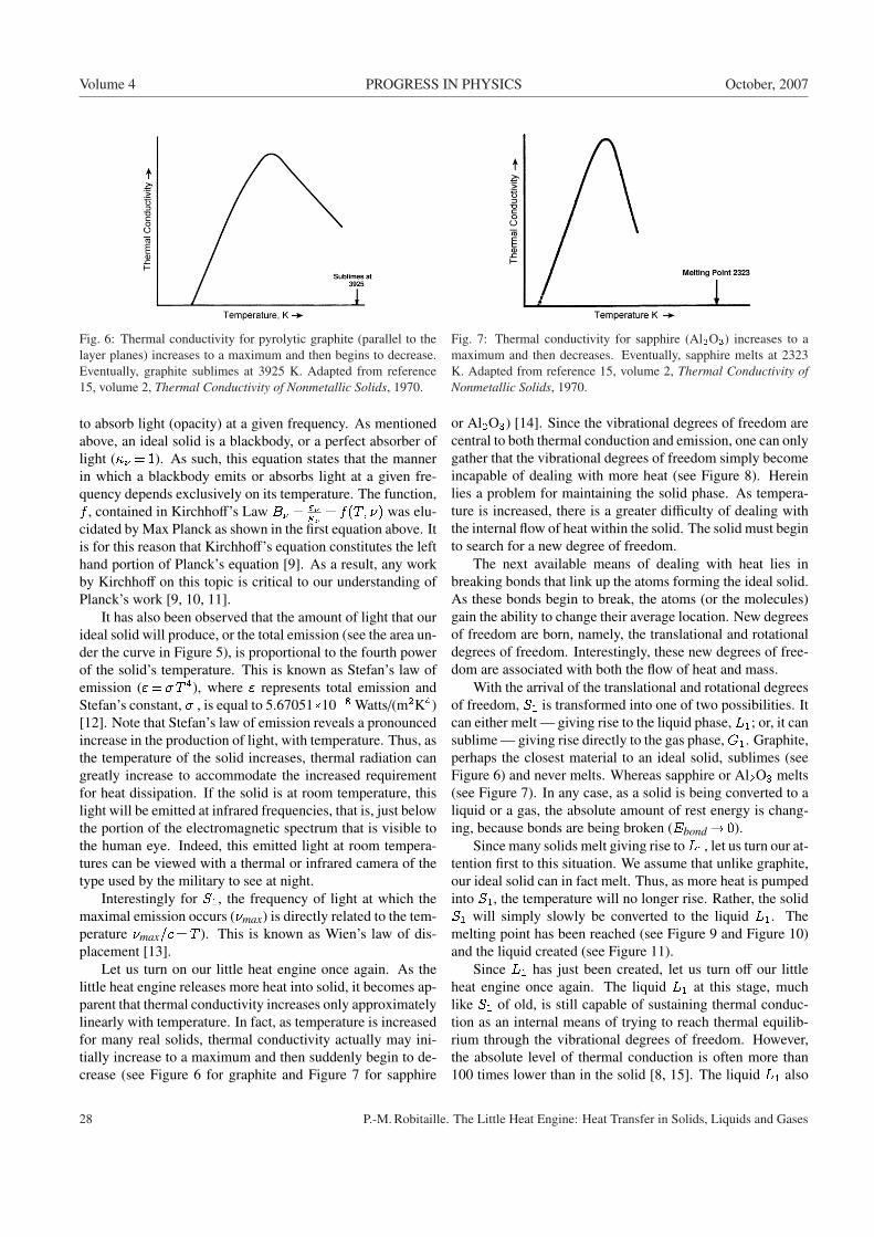
Volume 4 PROGRESS IN PHYSICS October, 2007
Fig. 6: Thermal conductivity for pyrolytic graphite (parallel to thelayer planes) increases to a maximum and then begins to decrease.Eventually, graphite sublimes at 3925 K. Adapted from reference15, volume 2, Thermal Conductivity of Nonmetallic Solids, 1970.
to absorb light (opacity) at a given frequency. As mentionedabove, an ideal solid is a blackbody, or a perfect absorber oflight (�� = 1). As such, this equation states that the mannerin which a blackbody emits or absorbs light at a given fre-quency depends exclusively on its temperature. The function,f , contained in Kirchhoff’s Law B� = "�
�� = f(T; �) was elu-cidated by Max Planck as shown in the first equation above. Itis for this reason that Kirchhoff’s equation constitutes the lefthand portion of Planck’s equation [9]. As a result, any workby Kirchhoff on this topic is critical to our understanding ofPlanck’s work [9, 10, 11].
It has also been observed that the amount of light that ourideal solid will produce, or the total emission (see the area un-der the curve in Figure 5), is proportional to the fourth powerof the solid’s temperature. This is known as Stefan’s law ofemission ("=�T 4), where " represents total emission andStefan’s constant, � , is equal to 5.67051�10�8 Watts/(m2K4)[12]. Note that Stefan’s law of emission reveals a pronouncedincrease in the production of light, with temperature. Thus, asthe temperature of the solid increases, thermal radiation cangreatly increase to accommodate the increased requirementfor heat dissipation. If the solid is at room temperature, thislight will be emitted at infrared frequencies, that is, just belowthe portion of the electromagnetic spectrum that is visible tothe human eye. Indeed, this emitted light at room tempera-tures can be viewed with a thermal or infrared camera of thetype used by the military to see at night.
Interestingly for S1, the frequency of light at which themaximal emission occurs (�max) is directly related to the tem-perature �max=c=T ). This is known as Wien’s law of dis-placement [13].
Let us turn on our little heat engine once again. As thelittle heat engine releases more heat into solid, it becomes ap-parent that thermal conductivity increases only approximatelylinearly with temperature. In fact, as temperature is increasedfor many real solids, thermal conductivity actually may ini-tially increase to a maximum and then suddenly begin to de-crease (see Figure 6 for graphite and Figure 7 for sapphire
Fig. 7: Thermal conductivity for sapphire (Al2O3) increases to amaximum and then decreases. Eventually, sapphire melts at 2323K. Adapted from reference 15, volume 2, Thermal Conductivity ofNonmetallic Solids, 1970.
or Al2O3) [14]. Since the vibrational degrees of freedom arecentral to both thermal conduction and emission, one can onlygather that the vibrational degrees of freedom simply becomeincapable of dealing with more heat (see Figure 8). Hereinlies a problem for maintaining the solid phase. As tempera-ture is increased, there is a greater difficulty of dealing withthe internal flow of heat within the solid. The solid must beginto search for a new degree of freedom.
The next available means of dealing with heat lies inbreaking bonds that link up the atoms forming the ideal solid.As these bonds begin to break, the atoms (or the molecules)gain the ability to change their average location. New degreesof freedom are born, namely, the translational and rotationaldegrees of freedom. Interestingly, these new degrees of free-dom are associated with both the flow of heat and mass.
With the arrival of the translational and rotational degreesof freedom, S1 is transformed into one of two possibilities. Itcan either melt — giving rise to the liquid phase, L1; or, it cansublime — giving rise directly to the gas phase,G1. Graphite,perhaps the closest material to an ideal solid, sublimes (seeFigure 6) and never melts. Whereas sapphire or Al2O3 melts(see Figure 7). In any case, as a solid is being converted to aliquid or a gas, the absolute amount of rest energy is chang-ing, because bonds are being broken (Ebond! 0).
Since many solids melt giving rise toL1, let us turn our at-tention first to this situation. We assume that unlike graphite,our ideal solid can in fact melt. Thus, as more heat is pumpedinto S1, the temperature will no longer rise. Rather, the solidS1 will simply slowly be converted to the liquid L1. Themelting point has been reached (see Figure 9 and Figure 10)and the liquid created (see Figure 11).
Since L1 has just been created, let us turn off our littleheat engine once again. The liquid L1 at this stage, muchlike S1 of old, is still capable of sustaining thermal conduc-tion as an internal means of trying to reach thermal equilib-rium through the vibrational degrees of freedom. However,the absolute level of thermal conduction is often more than100 times lower than in the solid [8, 15]. The liquid L1 also
28 P.-M. Robitaille. The Little Heat Engine: Heat Transfer in Solids, Liquids and Gases
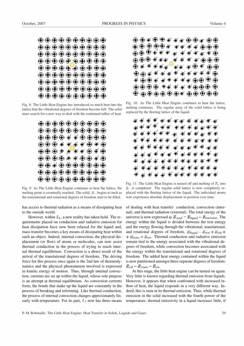
October, 2007 PROGRESS IN PHYSICS Volume 4
Fig. 8: The Little Heat Engine has introduced so much heat into thelattice that the vibrational degrees of freedom become full. The solidmust search for a new way to deal with the continued influx of heat.
Fig. 9: As The Little Heat Engine continues to heat the lattice, themelting point is eventually reached. The solid, S1, begins to melt asthe translational and rotational degrees of freedom start to be filled.
has access to thermal radiation as a means of dissipating heatto the outside world.
However, within L1, a new reality has taken hold. The re-quirements placed on conduction and radiative emission forheat dissipation have now been relaxed for the liquid and,mass transfer becomes a key means of dissipating heat withinsuch an object. Indeed, internal convection, the physical dis-placement (or flow) of atoms or molecules, can now assistthermal conduction in the process of trying to reach inter-nal thermal equilibrium. Convection is a direct result of thearrival of the translational degrees of freedom. The drivingforce for this process once again is the 2nd law of thermody-namics and the physical phenomenon involved is expressedin kinetic energy of motion. Thus, through internal convec-tion, currents are set up within the liquid, whose sole purposeis an attempt at thermal equilibrium. As convection currentsform, the bonds that make up the liquid are constantly in theprocess of breaking and reforming. Like thermal conduction,the process of internal convection changes approximately lin-early with temperature. For its part, L1 now has three means
Fig. 10: As The Little Heat Engine continues to heat the lattice,melting continues. The regular array of the solid lattice is beingreplaced by the fleeting lattice of the liquid.
Fig. 11: The Little Heat Engine is turned off and melting of S1 intoL1 is completed. The regular solid lattice is now completely re-placed with the fleeting lattice of the liquid. The individual atomsnow experience absolute displacement in position over time.
of dealing with heat transfer: conduction, convection (inter-nal), and thermal radiation (external). The total energy of theuniverse is now expressed asE total =Eliquid +Eemission. Theenergy within the liquid is divided between the rest energyand the energy flowing through the vibrational, translational,and rotational degrees of freedom, Eliquid =Erest +Evib ++Etrans +Erot. Thermal conduction and radiative emissionremain tied to the energy associated with the vibrational de-grees of freedom, while convection becomes associated withthe energy within the translational and rotational degrees offreedom. The added heat energy contained within the liquidis now partitioned amongst three separate degrees of freedom:Evib +E trans +Erot.
At this stage, the little heat engine can be turned on again.Very little is known regarding thermal emission from liquids.However, it appears that when confronted with increased in-flow of heat, the liquid responds in a very different way. In-deed, this is seen in its thermal emission. Thus, while thermalemission in the solid increased with the fourth power of thetemperature, thermal emissivity in a liquid increases little, if
P.-M. Robitaille. The Little Heat Engine: Heat Transfer in Solids, Liquids and Gases 29
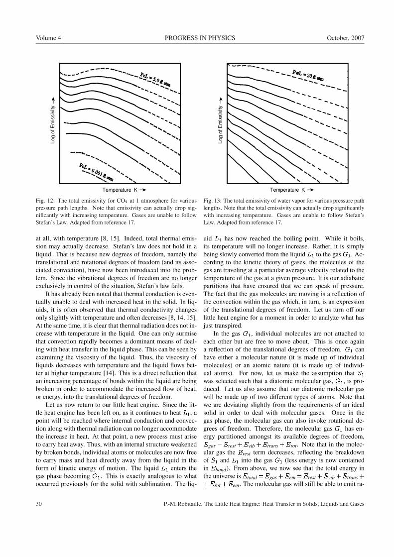
Volume 4 PROGRESS IN PHYSICS October, 2007
Fig. 12: The total emissivity for CO2 at 1 atmosphere for variouspressure path lengths. Note that emissivity can actually drop sig-nificantly with increasing temperature. Gases are unable to followStefan’s Law. Adapted from reference 17.
at all, with temperature [8, 15]. Indeed, total thermal emis-sion may actually decrease. Stefan’s law does not hold in aliquid. That is because new degrees of freedom, namely thetranslational and rotational degrees of freedom (and its asso-ciated convection), have now been introduced into the prob-lem. Since the vibrational degrees of freedom are no longerexclusively in control of the situation, Stefan’s law fails.
It has already been noted that thermal conduction is even-tually unable to deal with increased heat in the solid. In liq-uids, it is often observed that thermal conductivity changesonly slightly with temperature and often decreases [8, 14, 15].At the same time, it is clear that thermal radiation does not in-crease with temperature in the liquid. One can only surmisethat convection rapidly becomes a dominant means of deal-ing with heat transfer in the liquid phase. This can be seen byexamining the viscosity of the liquid. Thus, the viscosity ofliquids decreases with temperature and the liquid flows bet-ter at higher temperature [14]. This is a direct reflection thatan increasing percentage of bonds within the liquid are beingbroken in order to accommodate the increased flow of heat,or energy, into the translational degrees of freedom.
Let us now return to our little heat engine. Since the lit-tle heat engine has been left on, as it continues to heat L1, apoint will be reached where internal conduction and convec-tion along with thermal radiation can no longer accommodatethe increase in heat. At that point, a new process must ariseto carry heat away. Thus, with an internal structure weakenedby broken bonds, individual atoms or molecules are now freeto carry mass and heat directly away from the liquid in theform of kinetic energy of motion. The liquid L1 enters thegas phase becoming G1. This is exactly analogous to whatoccurred previously for the solid with sublimation. The liq-
Fig. 13: The total emissivity of water vapor for various pressure pathlengths. Note that the total emissivity can actually drop significantlywith increasing temperature. Gases are unable to follow Stefan’sLaw. Adapted from reference 17.
uid L1 has now reached the boiling point. While it boils,its temperature will no longer increase. Rather, it is simplybeing slowly converted from the liquid L1 to the gas G1. Ac-cording to the kinetic theory of gases, the molecules of thegas are traveling at a particular average velocity related to thetemperature of the gas at a given pressure. It is our adiabaticpartitions that have ensured that we can speak of pressure.The fact that the gas molecules are moving is a reflection ofthe convection within the gas which, in turn, is an expressionof the translational degrees of freedom. Let us turn off ourlittle heat engine for a moment in order to analyze what hasjust transpired.
In the gas G1, individual molecules are not attached toeach other but are free to move about. This is once againa reflection of the translational degrees of freedom. G1 canhave either a molecular nature (it is made up of individualmolecules) or an atomic nature (it is made up of individ-ual atoms). For now, let us make the assumption that S1was selected such that a diatomic molecular gas, G1, is pro-duced. Let us also assume that our diatomic molecular gaswill be made up of two different types of atoms. Note thatwe are deviating slightly from the requirements of an idealsolid in order to deal with molecular gases. Once in thegas phase, the molecular gas can also invoke rotational de-grees of freedom. Therefore, the molecular gas G1 has en-ergy partitioned amongst its available degrees of freedom,Egas =Erest +Evib +Etrans +Erot. Note that in the molec-ular gas the Erest term decreases, reflecting the breakdownof S1 and L1 into the gas G1 (less energy is now containedin Ebond). From above, we now see that the total energy inthe universe is Etotal =Egas +Eem =Erest +Evib +Etrans ++Erot +Eem. The molecular gas will still be able to emit ra-
30 P.-M. Robitaille. The Little Heat Engine: Heat Transfer in Solids, Liquids and Gases
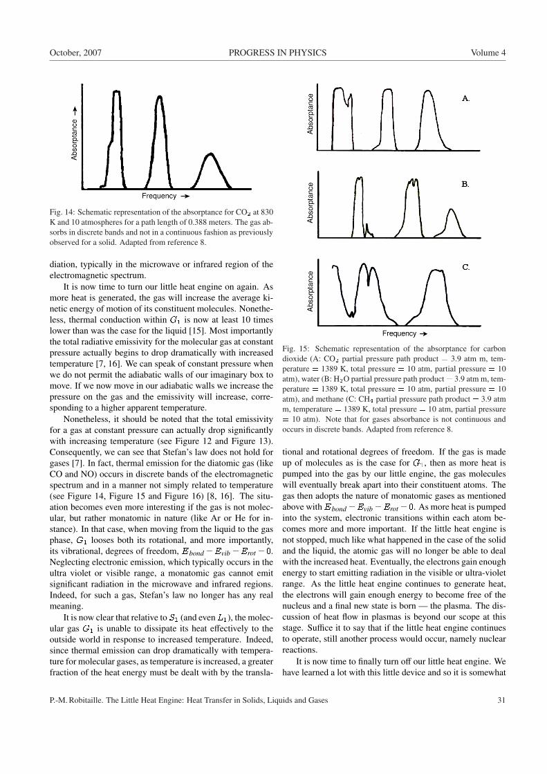
October, 2007 PROGRESS IN PHYSICS Volume 4
Fig. 14: Schematic representation of the absorptance for CO2 at 830K and 10 atmospheres for a path length of 0.388 meters. The gas ab-sorbs in discrete bands and not in a continuous fashion as previouslyobserved for a solid. Adapted from reference 8.
diation, typically in the microwave or infrared region of theelectromagnetic spectrum.
It is now time to turn our little heat engine on again. Asmore heat is generated, the gas will increase the average ki-netic energy of motion of its constituent molecules. Nonethe-less, thermal conduction within G1 is now at least 10 timeslower than was the case for the liquid [15]. Most importantlythe total radiative emissivity for the molecular gas at constantpressure actually begins to drop dramatically with increasedtemperature [7, 16]. We can speak of constant pressure whenwe do not permit the adiabatic walls of our imaginary box tomove. If we now move in our adiabatic walls we increase thepressure on the gas and the emissivity will increase, corre-sponding to a higher apparent temperature.
Nonetheless, it should be noted that the total emissivityfor a gas at constant pressure can actually drop significantlywith increasing temperature (see Figure 12 and Figure 13).Consequently, we can see that Stefan’s law does not hold forgases [7]. In fact, thermal emission for the diatomic gas (likeCO and NO) occurs in discrete bands of the electromagneticspectrum and in a manner not simply related to temperature(see Figure 14, Figure 15 and Figure 16) [8, 16]. The situ-ation becomes even more interesting if the gas is not molec-ular, but rather monatomic in nature (like Ar or He for in-stance). In that case, when moving from the liquid to the gasphase, G1 looses both its rotational, and more importantly,its vibrational, degrees of freedom, Ebond =Evib =Erot = 0.Neglecting electronic emission, which typically occurs in theultra violet or visible range, a monatomic gas cannot emitsignificant radiation in the microwave and infrared regions.Indeed, for such a gas, Stefan’s law no longer has any realmeaning.
It is now clear that relative to S1 (and evenL1), the molec-ular gas G1 is unable to dissipate its heat effectively to theoutside world in response to increased temperature. Indeed,since thermal emission can drop dramatically with tempera-ture for molecular gases, as temperature is increased, a greaterfraction of the heat energy must be dealt with by the transla-
Fig. 15: Schematic representation of the absorptance for carbondioxide (A: CO2 partial pressure path product = 3.9 atm m, tem-perature = 1389 K, total pressure = 10 atm, partial pressure = 10atm), water (B: H2O partial pressure path product = 3.9 atm m, tem-perature = 1389 K, total pressure = 10 atm, partial pressure = 10atm), and methane (C: CH4 partial pressure path product = 3.9 atmm, temperature = 1389 K, total pressure = 10 atm, partial pressure= 10 atm). Note that for gases absorbance is not continuous andoccurs in discrete bands. Adapted from reference 8.
tional and rotational degrees of freedom. If the gas is madeup of molecules as is the case for G1, then as more heat ispumped into the gas by our little engine, the gas moleculeswill eventually break apart into their constituent atoms. Thegas then adopts the nature of monatomic gases as mentionedabove withEbond =Evib =Erot = 0. As more heat is pumpedinto the system, electronic transitions within each atom be-comes more and more important. If the little heat engine isnot stopped, much like what happened in the case of the solidand the liquid, the atomic gas will no longer be able to dealwith the increased heat. Eventually, the electrons gain enoughenergy to start emitting radiation in the visible or ultra-violetrange. As the little heat engine continues to generate heat,the electrons will gain enough energy to become free of thenucleus and a final new state is born — the plasma. The dis-cussion of heat flow in plasmas is beyond our scope at thisstage. Suffice it to say that if the little heat engine continuesto operate, still another process would occur, namely nuclearreactions.
It is now time to finally turn off our little heat engine. Wehave learned a lot with this little device and so it is somewhat
P.-M. Robitaille. The Little Heat Engine: Heat Transfer in Solids, Liquids and Gases 31
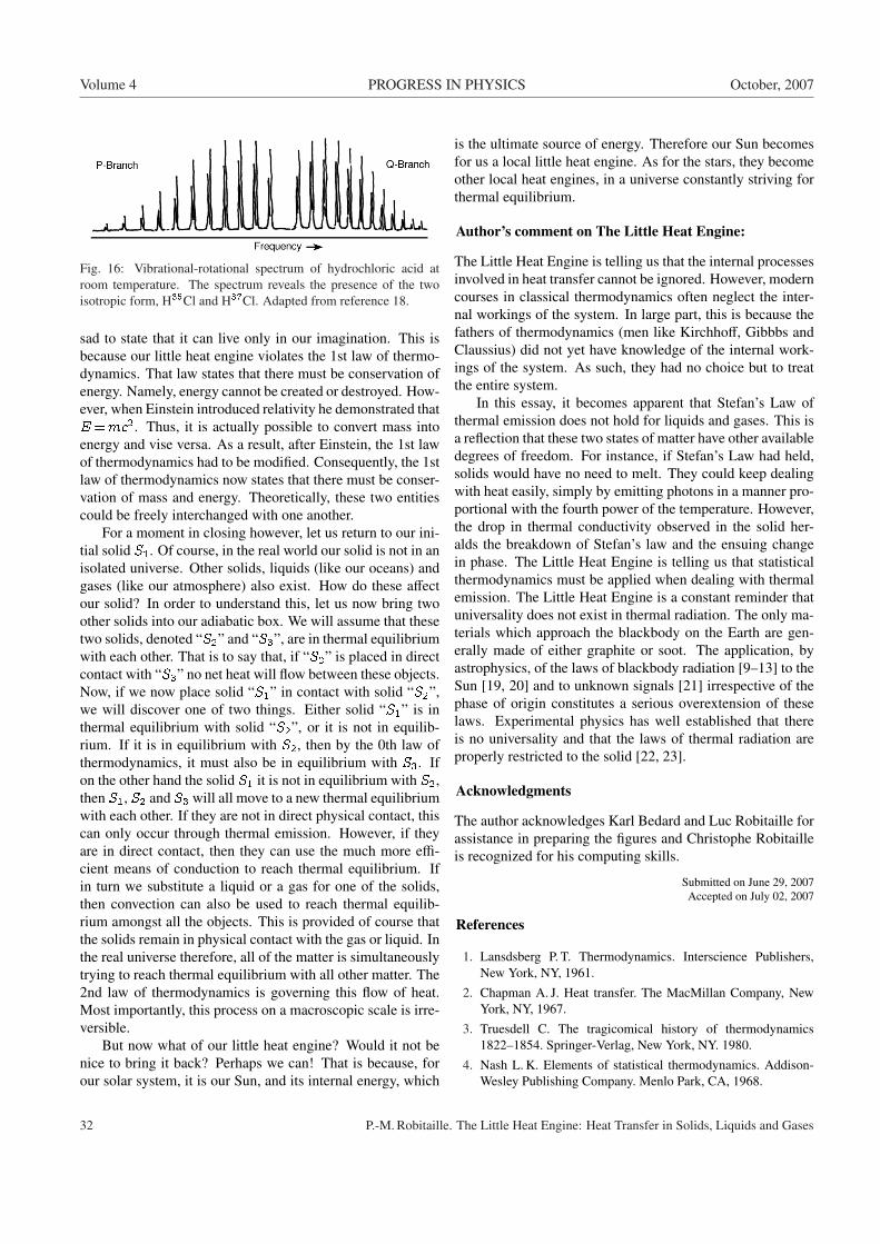
Volume 4 PROGRESS IN PHYSICS October, 2007
Fig. 16: Vibrational-rotational spectrum of hydrochloric acid atroom temperature. The spectrum reveals the presence of the twoisotropic form, H35Cl and H37Cl. Adapted from reference 18.
sad to state that it can live only in our imagination. This isbecause our little heat engine violates the 1st law of thermo-dynamics. That law states that there must be conservation ofenergy. Namely, energy cannot be created or destroyed. How-ever, when Einstein introduced relativity he demonstrated thatE=mc2. Thus, it is actually possible to convert mass intoenergy and vise versa. As a result, after Einstein, the 1st lawof thermodynamics had to be modified. Consequently, the 1stlaw of thermodynamics now states that there must be conser-vation of mass and energy. Theoretically, these two entitiescould be freely interchanged with one another.
For a moment in closing however, let us return to our ini-tial solid S1. Of course, in the real world our solid is not in anisolated universe. Other solids, liquids (like our oceans) andgases (like our atmosphere) also exist. How do these affectour solid? In order to understand this, let us now bring twoother solids into our adiabatic box. We will assume that thesetwo solids, denoted “S2” and “S3”, are in thermal equilibriumwith each other. That is to say that, if “S2” is placed in directcontact with “S3” no net heat will flow between these objects.Now, if we now place solid “S1” in contact with solid “S2”,we will discover one of two things. Either solid “S1” is inthermal equilibrium with solid “S2”, or it is not in equilib-rium. If it is in equilibrium with S2, then by the 0th law ofthermodynamics, it must also be in equilibrium with S3. Ifon the other hand the solid S1 it is not in equilibrium with S2,then S1, S2 and S3 will all move to a new thermal equilibriumwith each other. If they are not in direct physical contact, thiscan only occur through thermal emission. However, if theyare in direct contact, then they can use the much more effi-cient means of conduction to reach thermal equilibrium. Ifin turn we substitute a liquid or a gas for one of the solids,then convection can also be used to reach thermal equilib-rium amongst all the objects. This is provided of course thatthe solids remain in physical contact with the gas or liquid. Inthe real universe therefore, all of the matter is simultaneouslytrying to reach thermal equilibrium with all other matter. The2nd law of thermodynamics is governing this flow of heat.Most importantly, this process on a macroscopic scale is irre-versible.
But now what of our little heat engine? Would it not benice to bring it back? Perhaps we can! That is because, forour solar system, it is our Sun, and its internal energy, which
is the ultimate source of energy. Therefore our Sun becomesfor us a local little heat engine. As for the stars, they becomeother local heat engines, in a universe constantly striving forthermal equilibrium.
Author’s comment on The Little Heat Engine:
The Little Heat Engine is telling us that the internal processesinvolved in heat transfer cannot be ignored. However, moderncourses in classical thermodynamics often neglect the inter-nal workings of the system. In large part, this is because thefathers of thermodynamics (men like Kirchhoff, Gibbbs andClaussius) did not yet have knowledge of the internal work-ings of the system. As such, they had no choice but to treatthe entire system.
In this essay, it becomes apparent that Stefan’s Law ofthermal emission does not hold for liquids and gases. This isa reflection that these two states of matter have other availabledegrees of freedom. For instance, if Stefan’s Law had held,solids would have no need to melt. They could keep dealingwith heat easily, simply by emitting photons in a manner pro-portional with the fourth power of the temperature. However,the drop in thermal conductivity observed in the solid her-alds the breakdown of Stefan’s law and the ensuing changein phase. The Little Heat Engine is telling us that statisticalthermodynamics must be applied when dealing with thermalemission. The Little Heat Engine is a constant reminder thatuniversality does not exist in thermal radiation. The only ma-terials which approach the blackbody on the Earth are gen-erally made of either graphite or soot. The application, byastrophysics, of the laws of blackbody radiation [9–13] to theSun [19, 20] and to unknown signals [21] irrespective of thephase of origin constitutes a serious overextension of theselaws. Experimental physics has well established that thereis no universality and that the laws of thermal radiation areproperly restricted to the solid [22, 23].
Acknowledgments
The author acknowledges Karl Bedard and Luc Robitaille forassistance in preparing the figures and Christophe Robitailleis recognized for his computing skills.
Submitted on June 29, 2007Accepted on July 02, 2007
References
1. Lansdsberg P. T. Thermodynamics. Interscience Publishers,New York, NY, 1961.
2. Chapman A. J. Heat transfer. The MacMillan Company, NewYork, NY, 1967.
3. Truesdell C. The tragicomical history of thermodynamics1822–1854. Springer-Verlag, New York, NY. 1980.
4. Nash L. K. Elements of statistical thermodynamics. Addison-Wesley Publishing Company. Menlo Park, CA, 1968.
32 P.-M. Robitaille. The Little Heat Engine: Heat Transfer in Solids, Liquids and Gases

October, 2007 PROGRESS IN PHYSICS Volume 4
5. Buchdahl H. A. Twenty lectures on thermodynamics. PergamonPress, Oxford, UK, 1975.
6. Wilson A. H. Thermodynamics and statistical mechanics. Cam-bridge University Press, Cambridge, UK, 1961.
7. Knudsen J. G., Bell K. J., Holt A. D., Hottel H. C., SarofimA. F., Standiford F. C., Stuhlbarg D. and Uhl V. W. Heat trans-mission. In: Perry’s Chemical Engineer’s Handbook SixthEdition (R. H. Perry, D. W. Green and J. O. Maloney, Eds.)McGraw-Hill Book Company, New York, p. 10.1–10.68, 1984.
8. Siegel R. and Howell J. R. Thermal radiation heat transfer(3rd Edition). Hemisphere Publishing Corporation, Washing-ton, DC, 1992.
9. Planck M. Ueber das Gesetz der Energieverteilung in Normal-spectrum. Annalen der Physik, 1901, v. 4, 553–563.
10. Kirchhoff G. Ueber den Zusammenhang von Emission und Ab-sorption von Licht und Warme. Monatsberichte der Akademieder Wissenschaften zu Berlin, sessions of Dec. 1859, 783–787.
11. Kirchhoff G. Ueber das Verhaltnis zwischen dem Emissionsver-mogen und dem Absorptionsvermogen der Korper fur Warmeund Licht. Annalen der Physik, 1860, v. 109, 275–301.
12. Stefan J. Ueber die Beziehung zwischen der Warmestrahlungund der Temperatur. Wein. Akad. Sitzber., 1879, v. 79, 391–428.
13. Wien W. Uber die Energieverteilung im Emissionspektrumeines schwarzen Korpers. Annalen der Physik, 1896, v. 58,662–669.
14. Touloukian Y. S. and Ho C. Y. Thermophysical Properties ofMatter (vols. 1–8). Plenum, New York, 1970.
15. Vargaftik N. B., Filippov L. D., Tarzimanov A. A. and TotskiiE. E. Handbook of thermal conductivities of liquids and gases.CRC Press, Boca Raton, FL, 1994.
16. Penner S. S. Quantitative molecular spectroscopy and gas emis-sivities. Addison-Wesley Publishing Company Inc., Reading,MA, 1959.
17. DeWitt D. P. and Nutter G. D. Theory and practice of radiationthermometry. John Wiley and Sons Inc., New York, NY, 1988.
18. Gasser R. P. H. and Richards W. G. An introduction to statisticalthermodynamics. World Scientific, London, UK, 1995.
19. Langley S. P. Experimental determination of wave-lengths inthe invisible spectrum. Mem. Natl. Acad. Sci., 1883, v. 2, 147–162.
20. Langley S. P. On hitherto unrecognized wave-lengths. Phil.Mag., 1886, v. 22, 149–173.
21. Penzias A. A. and Wilson R. W. A measurement of excess an-tenna temperature at 4080 Mc/s. Astrophysical J., 1965, v. 1,419–421.
22. Robitaille P.-M. L. On the validity of Kirchhoff’s law of thermalemission. IEEE Trans. Plasma Sci., 2003, v. 31(6), 1263.
23. Robitaille P.-M. L. An analysis of universality in blackbody ra-diation. Progr. Phys., 2006, v. 2, 22–23.
P.-M. Robitaille. The Little Heat Engine: Heat Transfer in Solids, Liquids and Gases 33
Volume 4 PROGRESS IN PHYSICS October, 2007
SPECIAL REPORT
A Four-Dimensional Continuum Theory of Space-Time andthe Classical Physical Fields
Indranu Suhendro
Department of Physics, Karlstad University, Karlstad 651 88, SwedenE-mail: spherical [email protected]
In this work, we attempt to describe the classical physical fields of gravity, electromag-netism, and the so-called intrinsic spin (chirality) in terms of a set of fully geometrizedconstitutive equations. In our formalism, we treat the four-dimensional space-time con-tinuum as a deformable medium and the classical fields as intrinsic stress and spin fieldsgenerated by infinitesimal displacements and rotations in the space-time continuum it-self. In itself, the unifying continuum approach employed herein may suggest a possibleunified field theory of the known classical physical fields.
1 Introduction
Many attempts have been made to incorporate the so-calledstandard (Hookean) linear elasticity theory into general rela-tivity in the hope to describe the dynamics of material bodiesin a fully covariant four-dimensional manner. As we know,many of these attempts have concentrated solely on the treat-ment of material bodies as linearly elastic continua and notquite generally on the treatment of space-time itself as a lin-early elastic, deformable continuum. In the former case, tak-ing into account the gravitational field as the only intrinsicfield in the space-time continuum, it is therefore true thatthe linearity attributed to the material bodies means that thegeneral consideration is limited to weakly gravitating objectsonly. This is because the curvature tensor is in general quad-ratic in the the so-called connection which can be said torepresent the displacement field in the space-time manifold.However, in most cases, it is enough to consider an infinitesi-mal displacement field only such that the linear theory worksperfectly well. However, for the sake of generality, we neednot assume only the linear behavior of the properly-stressedspace-time continuum (and material bodies) such that the pos-sible limiting consequences of the linear theory can be readilyovercome whenever it becomes necessary. Therefore, in thepresent work, we shall both consider both the linear and non-linear formulations in terms of the response of the space-timegeometry to infinitesimal deformations and rotations with in-trinsic generators.
A few past attempts at the full description of the elas-tic behavior of the space-time geometry in the presence ofphysical fields in the language of general relativity have beenquite significant. However, as standard general relativity de-scribes only the field of gravity in a purely geometric fash-ion, these past attempts have generally never gone beyondthe simple reformulation of the classical laws of elasticity inthe presence of gravity which means that these classical lawsof elasticity have merely been referred to the general four-
dimensional curvilinear coordinates of Riemannian geome-try, nothing more. As such, any possible interaction betweenthe physical fields (e.g., the interaction between gravity andelectromagnetism) has not been investigated in detail.
In the present work, we develop a fully geometrized con-tinuum theory of space-time and the classical physical fieldsin which the actions of these physical fields contribute di-rectly to the dynamics of the space-time geometry itself. Inthis model, we therefore assume that a physical field is di-rectly associated with each and every point in the region ofspace-time occupied by the field (or, a material body in thecase of gravity). This allows us to describe the dynamics ofthe space-time geometry solely in terms of the translationaland rotational behavior of points within the occupied region.Consequently, the geometric quantities (objects) of the space-time continuum (e.g., curvature) are directly describable interms of purely kinematic variables such as displacement,spin, velocity, acceleration, and the particle symmetries them-selves.
As we have said above, at present, for the sake of sim-plicity, we shall assume the inherently elastic behavior of thespace-time continuum. This, I believe, is adequate especiallyin most cosmological cases. Such an assumption is nothingbut intuitive, especially when considering the fact that wedo not fully know the reality of the constituents of the fab-ric of the Universe yet. As such, the possible limitations ofthe present theory, if any, can be neglected considerably untilwe fully understand how the fabric of the space-time contin-uum is actually formed and how the properties of individualelementary particles might contribute to this formation.
2 The fundamental geometric properties of a curvedmanifold
Let us present the fundamental geometric objects of an n-dimensional curved manifold. Let !a = @Xi
@xa Ei = @aXiEi(the Einstein summation convention is assumed throughout
34 I. Suhendro. A Four-Dimensional Continuum Theory of Space-Time and the Classical Physical Fields
October, 2007 PROGRESS IN PHYSICS Volume 4
this work) be the covariant (frame) basis spanning the n-dimensional base manifold C1 with local coordinates xa ==xa
�Xk�. The contravariant (coframe) basis �b is then given
via the orthogonal projection�b; !a
�= �ba, where �ba are the
components of the Kronecker delta (whose value is unity ifthe indices coincide or null otherwise). The set of linearly in-dependent local directional derivatives Ei = @
@Xi = @i givesthe coordinate basis of the locally flat tangent space Tx(M)at a point x 2 C1. Here M denotes the topological space ofthe so-called n-tuples h (x) =h
�x1; : : : ; xn
�such that rel-
ative to a given chart (U; h (x)) on a neighborhood U of alocal coordinate point, our C1-differentiable manifold itselfis a topological space. The dual basis to Ei spanning the lo-cally flat cotangent space T�x(M) will then be given by thedifferential elements dXk via the relation
dXk; @i
�= �ki .
In fact and in general, the one-forms dXk indeed act as alinear map Tx(M)! IR when applied to an arbitrary vectorfield F 2 Tx(M) of the explicit form F =F i @
@Xi = fa @@xa .
Then it is easy to see that F i =F Xi and fa =F xa, fromwhich we obtain the usual transformation laws for the con-travariant components of a vector field, i.e., F i = @aXifaand f i = @ixaF i, relating the localized components of F tothe general ones and vice versa. In addition, we also see thatdXk; F
�=FXk =F k.
The components of the symmetric metric tensor g== gab �a �b of the base manifold C1 are readily given by
gab = h!a; !bisatisfying
gac gbc = �ba
where gab =�a; �b
�. It is to be understood that the covari-
ant and contravariant components of the metric tensor willbe used to raise and the (component) indices of vectors andtensors.
The components of the metric tensor
g (xN ) = �ik dXi dXk
describing the locally flat tangent space Tx(M) of rigidframes at a point xN =xN (xa) are given by
�ik = hEi; Eki = diag (�1;�1; : : : ;�1) :
In four dimensions, the above may be taken to be the com-ponents of the Minkowski metric tensor, i.e., �ik=hEi; Eki== diag (1;�1;�1;�1).
Then we have the expression
gab = �ik @aXi@bXk:
The line-element of C1 is then given by
ds2 = g = gab�@ixa@kxb
�dXi dXk
where �a = @ixadXi.
Given the existence of a local coordinate transformationvia xi = xi (x�) in C1, the components of an arbitrary ten-sor field T 2 C1 of rank (p; q) transform according to
T ab:::gcd:::h = T��:::���:::� @�xa @� xb : : : @�xg @c �x� @d �x� : : : @h �x�:
Let �i1i2:::ipj1j2:::jp be the components of the generalized Kro-necker delta. They are given by
�i1i2:::ipj1j2:::jp =2j1j2:::jp2i1:::ip= det
0BBB@�i1j1 �i2j1 : : : �ipj1�i1j2 �i2j2 : : : �ipj2: : : : : : : : : : : :�i1jp �i2jp : : : �ipjp
1CCCAwhere 2j1j2:::jp =
pdet (g) �j1j2:::jp and 2i1i2:::ip = �i1i2:::ipp
det(g)are the covariant and contravariant components of the com-pletely anti-symmetric Levi-Civita permutation tensor, re-spectively, with the ordinary permutation symbols beinggiven as usual by �j1j2:::jq and �i1i2:::ip . Again, if ! is anarbitrary tensor, then the object represented by
�!j1j2:::jp =1p!�i1i2:::ipj1j2:::jp !i1i2:::ip
is completely anti-symmetric.Introducing a generally asymmetric connection � via the
covariant derivative
@b!a = �cab!ci.e.,
�cab = h�c; @b!ai = �c(ab) + �c[ab]
where the round index brackets indicate symmetrization andthe square ones indicate anti-symmetrization, we have, bymeans of the local coordinate transformation given by xa ==xa (�x�) in C1
@b e�a = �cab e�c � ����� e
�a e
�b
where the tetrads of the moving frames are given by e�a == @a�x� and ea� = @�xa. They satisfy ea�e�b = �ab and e�aea� == ��� . In addition, it can also be verified that
@� ea� = ����� ea� � �abc eb� ec� ;
@b ea� = ea� ����� e�b � �acb ec� :
We know that � is a non-tensorial object, since its com-ponents transform as
�cab = ec�@be�a + ec� ����� e
�a e
�b :
However, it can be described as a kind of displacementfield since it is what makes possible a comparison of vectorsfrom point to point in C1. In fact the relation @b!a = �cab!c
I. Suhendro. A Four-Dimensional Continuum Theory of Space-Time and the Classical Physical Fields 35
Volume 4 PROGRESS IN PHYSICS October, 2007
defines the so-called metricity condition, i.e., the change (dur-ing a displacement) in the basis can be measured by the basisitself. This immediately translates into
rc gab = 0
where we have just applied the notion of a covariant derivativeto an arbitrary tensor field T :
rmT ab:::gcd:::h = @mTab:::gcd:::h + �apmT
pb:::gcd:::h + �bpmT
ap:::gcd:::h + : : :
: : :+ �gpmT ab:::pcd:::h � �pcmT ab:::gpd:::h � �pdmTab:::gcp:::h � : : :
: : :� �phmTab:::gcd:::p
such that (@mT )ab:::gcd:::h = rm T ab:::gcd:::h .The condition rcgab = 0 can be solved to give
�cab =12gcd (@b gda � @d gab + @a gbd) +
+ �c[ab] � gcd�gae�e[db] + gbe�e[da]
�from which it is customary to define
�cab =
12gcd (@b gda � @d gab + @a gbd)
as the Christoffel symbols (symmetric in their two lower in-dices) and
Kcab = �c[ab] � gcd
�gae�e[db] + gbe�e[da]
�as the components of the so-called cotwist tensor (anti-symmetric in the first two mixed indices).
Note that the components of the twist tensor are given by
�a[bc] =12ea��@c e�b � @b e�c + e�b ����c � e�c ����b
�where we have set ����c = �����e�c , such that for an arbitraryscalar field � we have
(rarb �rbra) � = 2�c[ab]rc� :
The components of the curvature tensorR of C1 are thengiven via the relation
(rqrp �rprq)T ab:::scd:::r = T ab:::swd:::rRwcpq + T ab:::scw:::rR
wdpq +
+ : : :+ T ab:::scd:::wRwrpq � Twb:::scd:::r R
awpq � T aw:::scd:::r R
bwpq �
� : : :� T ab:::wcd:::r Rswpq � 2�w[pq]rw T ab:::scd:::r
where
Rdabc = @b�dac � @c�dab + �eac�deb � �eab�
dec
= Bdabc (�) + rbKdac � rcKd
ab +KeacK
deb �Ke
abKdec ;
where r denotes covariant differentiation with respect to theChristoffel symbols alone, and where
Bdabc (�) = @b�dac � @c�d
ab + �eac�
deb ��e
ab�dec
are the components of the Riemann-Christoffel curvature ten-sor of C1.
From the components of the curvature tensor, namely,Rdabc, we have (using the metric tensor to raise and lowerindices)
Rab � Rcacb = Bab (�) + rcKcab �Kc
adKdcb�
� 2rb�c[ac] + 2Kcab�
d[cd]
R � Raa = B (�)� 4gab ra�c[bc]�� 2gac�b[ab]�
d[cd] �KabcKacb
where Bab (�) � Bcacb (�) are the components of the sym-metric Ricci tensor and B (�) � Baa (�) is the Ricci scalar.Note that Kabc � gadKd
bc and Kacb � gcdgbeKade.
Now since
�bba = �bba = �b
ab = @a�
lnp
det (g)�
�bab = @a�
lnp
det (g)�
+ 2�b[ab]
we see that for a continuous metric determinant, the so-calledhomothetic curvature vanishes:
Hab � Rccab = @a�ccb � @b�cca = 0 :
Introducing the traceless Weyl tensorW , we have the fol-lowing decomposition theorem:
Rdabc =W dabc+
1n�2
��dbRac+gacR
db��dcRab�gabRdc�+
+1
(n� 1) (n� 2)��dc gab � �db gac�R
which is valid for n > 2. For n = 2, we have
Rdabc = KG��db gac � �dc gab�
whereKG =
12R
is the Gaussian curvature of the surface. Note that (in thiscase) the Weyl tensor vanishes.
Any n-dimensional manifold (for which n > 1) with con-stant sectional curvature R and vanishing twist is called anEinstein space. It is described by the following simple rela-tions:
Rdabc =1
n(n� 1)��db gac � �dc gab�R ;
Rab =1ngabR :
36 I. Suhendro. A Four-Dimensional Continuum Theory of Space-Time and the Classical Physical Fields
October, 2007 PROGRESS IN PHYSICS Volume 4
In the above, we note especially that
Rdabc = Bdabc (�) ;
Rab = Bab (�) ;
R = B (�) :
Furthermore, after some lengthy algebra, we obtain, ingeneral, the following generalized Bianchi identities:
Rabcd +Racdb +Radbc = �2�@d�a[bc] + @b�a[cd] +
+ @c�a[db] + �aeb�e[cd] + �aec�
e[db] + �aed�
e[bc]�;
reRabcd +rcRabde +rdRabec =
= 2��f[cd]R
abfe + �f[de]R
abfc + �f[ec]R
abfd�;
ra�Rab � 1
2gabR
�= 2gab�c[da]R
dc + �a[cd]R
cdba
for any metric-compatible manifold endowed with both cur-vature and twist.
In the last of the above set of equations, we have intro-duced the generalized Einstein tensor, i.e.,
Gab � Rab � 12gabR
In particular, we also have the following specialized iden-tities, i.e., the regular Bianchi identities:
Babcd +Bacdb +Badbc = 0 ;
reBabcd + rcBabde + rdBabec = 0 ;
ra�Bab � 1
2gabB
�= 0 :
In general, these hold in the case of a symmetric, metric-compatible connection. Non-metric differential geometry isbeyond the scope of our present consideration.
We now define the so-called Lie derivative which can beused to define a diffeomorphism invariant in C1. for a vec-tor field U and a tensor field T , both arbitrary, the invariantderivative represented (in component notation) by
LUTab:::gcd:::h = @mT
ab:::gcd:::h U
m + T ab:::gmd:::h @cUm +
+ T ab:::gcm:::h @dUm + : : :+ T ab:::gcd:::m @hU
m�� Tmb:::gcd:::h @mUa � T am:::gcd::::h @mU
b � : : :� T ab:::mcd:::h @mUg
defines the Lie derivative of T with respect to U . With thehelp of the twist tensor and the relation
@bUa = rbUa � �acbUc = rbUa � ��abc � 2�a[bc]
�Uc
we can write
LUTab:::gcd:::h = rmT ab:::gcd:::h U
m + T ab:::gmd:::hrcUm +
+ T ab:::gcm:::hrdUm + : : :+ T ab:::gcd:::mrhUm � Tmb:::gcd:::h rmUa�� T am:::gcd::::h rmU b � : : :� T ab:::mcd:::h rmUg +
+ 2�a[mp]Tmb:::gcd:::h Up + 2�b[mp]T
am:::gcd:::h Up +
: : : + 2�g[mp]Tab:::mcd:::h Up � 2�m[cp]T
ab:::gmd:::hU
p +
+ 2�m[dp]Tab:::gcm:::hU
p � : : :� 2�m[hp]Tab:::gcd:::mU
p:
Hence, noting that the components of the twist tensor,namely, �i[kl], indeed transform as components of a tensor
field, it is seen that the LUTij:::skl:::r do transform as components
of a tensor field. Apparently, the beautiful property of theLie derivative (applied to an arbitrary tensor field) is that it isconnection-independent even in a curved manifold.
We will need the identities derived in this Section later on.
3 The generalized four-dimensional linear constitutivefield equations
We shall now present a four-dimensional linear continuumtheory of the classical physical fields capable of describingmicrospin phenomena in addition to the gravitational andelectromagnetic fields. By microspin phenomena, we meanthose phenomena generated by rotation of points in the four-dimensional space-time manifold (continuum) S4 with localcoordinates x� in the manner described by the so-calledCosserat continuum theory.
We start with the following constitutive equation in fourdimensions:
T�� = C����D�� =
1�
�R�� � 1
2g��R
�where now the Greek indices run from 0 to 3. In the aboveequation, T�� are the contravariant components of the gener-ally asymmetric energy-momentum tensor, C���� are themixed components of the generalized four-dimensional elas-ticity tensor, D�� are the contravariant components of thefour-dimensional displacement gradient tensor, R�� are thecontravariant components of the generalized (asymmetric)four-dimensional Ricci curvature tensor, �=�8� is the Ein-stein coupling constant (in geometrized units), and R=R�� isthe generalized Ricci four-dimensional curvature scalar.
Furthermore, we can decompose our four-dimensionalelasticity tensor into its holonomic and anholonomic parts asfollows:
C���� = A���� +B����where
A���� = A(��)(��) = A����
B���� = B[��][��] = B����
I. Suhendro. A Four-Dimensional Continuum Theory of Space-Time and the Classical Physical Fields 37
Volume 4 PROGRESS IN PHYSICS October, 2007
such thatC���� = C ��
�� :
Therefore, we can express the fully covariant componentsof the generalized four-dimensional elasticity tensor in termsof the covariant components of the symmetric metric tensorg�� (satisfying, as before, g��g�� = ��� ) as
C���� = �g��g�� + �g��g�� + g��g�� =
= �g��g��+� (g��g��+g��g��) + ! (g��g���g��g��)where �, �, , �, and ! are constitutive invariants that are notnecessarily constant. It is therefore seen that
A���� = �g��g�� + � (g��g�� + g��g��)
B���� = ! (g��g�� � g��g��)An infinitesimal displacement (diffeomorphism) in the
space-time manifold S4 from an initial point P to a neigh-boring point Q is given as usual by
x� (Q) = x�(P ) + ��
where �� are the components of the four-dimensional infinite-simal displacement field vector. The generally asymmetricfour-dimensional displacement gradient tensor is then givenby
D�� = r� �� :The decomposition D�� = D(��) + D[��] and the sup-
plementary infinitesimal point-rotation condition ��[��]�� = 0
allow us to define the symmetric four-dimensional displace-ment (“dilation”) tensor by
��� = D(��) =12
(r��� +r���) =12L� g��
from which the “dilation” scalar is given by
� = ��� = D�� =
12g�� L� g�� = r� ��
as well as the anti-symmetric four-dimensional intrinsic spin(vorticity) tensor by
!�� = D[��] =12
(r� �� �r� ��) :
Let us now decompose the four-dimensional infinitesimaldisplacement field vector as follows:
�� = @�F + �:
Here the continuous scalar function F represents the in-tegrable part of the four-dimensional macroscopic displace-ment field vector while the remaining parts are given by � via
� = �� + �� + 2 �e'�
where �� are the components of the non-integrable four-
dimensional macroscopic displacement field vector, �� arethe components of the four-dimensional microscopic (micro-polar) intrinsic spin vector, e is a constant proportional to theelectric charge, and '� are the components of the electromag-netic four-potential vector. We assume that in general ��, ��,and '� are linearly independent of each other.
The intrinsic four-dimensional macroscopic spin (“angu-lar momentum”) tensor is then given by
�� =12
(r� �� �r� ��) :
Likewise, the intrinsic four-dimensional microscopic (mi-cropolar) spin tensor is given by
S�� =12
(r� �� �r� ��) :
Note that this tensor vanishes when the points are not al-lowed to rotate such as in conventional (standard) cases.
Meanwhile, the electromagnetic field tensor is given by
F�� = r� '� �r� '� :In this case, we especially note that, by means of the con-
dition ��[��]�� = 0, the above expression reduces to the usual
Maxwellian relation
F�� = @�'� � @�'� :We can now write the intrinsic spin tensor as
!�� = �� + S�� + �eF�� :
Hence the full electromagnetic content of the theory be-comes visible. We also see that our space-time continuum canbe considered as a dynamically polarizable medium possess-ing chirality. As such, the gravitational and electromagneticfields, i.e., the familiar classical fields, are intrinsic geometricobjects in the theory.
Furthermore, from the cotwist tensor, let us define a geo-metric spin vector via
A� � K��� = 2��[��]:
Now, in a somewhat restrictive case, in connection withthe spin fields represented by ��; ��; and '�, the selection
A� = c1�� + c2�� + 2 �ec3'� = 2 �i.e.,
2 =c1�� + c2�� + 2 �ec3'��� + �� + 2 �e'�
will directly attribute the cotwist tensor to the intrinsic spinfields of the theory. However, we would in general expect theintrinsic spin fields to remain in the case of a semi-symmetricconnection, for which A� = 0 and so we cannot carry thisproposition any further.
38 I. Suhendro. A Four-Dimensional Continuum Theory of Space-Time and the Classical Physical Fields
October, 2007 PROGRESS IN PHYSICS Volume 4
At this point, we see that the holonomic part of the gen-eralized four-dimensional elasticity tensor given by A���� isresponsible for (centrally symmetric) gravitational phenom-ena while the anholonomic part given by B���� owes its ex-istence to the (con)twist tensor which is responsible for theexistence of the intrinsic spin fields in our consideration.
Furthermore, we see that the components of the energy-momentum tensor can now be expressed as
T�� = �g��� + �D�� + D�� :
In other words,
T(��) = �g��� + (� + ) ��� ;
T[��] = (� � )!�� :
Alternatively,
T(��) =12�g��g��L� g�� +
12
(� + )L� g�� ;
T[��] = (� � ) (�� + S�� + �eF��) :
We may note that, in a sense analogous to that of the or-dinary mechanics of continuous media, the generally asym-metric character of the energy-momentum tensor means thata material object in motion is generally subject to distributedbody couples.
We also have
T = T�� = (4�+ � + ) � = � 1�R :
Let us briefly relate our description to the standard mate-rial description given by general relativity. For this purpose,let us assume that the intrinsic spin fields other than the elec-tromagnetic field are negligible. If we denote the materialdensity and the pressure by � and p, respectively, then it canbe directly verified that
� =�� 4p
4�+ � + is a solution to the ordinary expression
T(��) = �u�u� � pg�� �� 1
4�
�F��F �� � 1
4g��F��F��
�where u� are the covariant components of the unit veloc-ity vector. This is true whether the electromagnetic field ispresent or not since the (symmetric) energy-momentum ten-sor of the electromagnetic field given by
J�� = � 14�
�F��F �� � 1
4g��F��F��
�is traceless.
At this point, however, we may note that the covariant
divergence
r� T�� = g��r� (��) + �r�D�� +
+ r�D�� +D��r� � +D��r� need not vanish in general since
r� T�� =1�r��R�� � 1
2g��R
�=
=1�
�2g�� ��[��]R
�� + ��[��]R
����
�:
In an isotropic, homogeneous Universe, for which theconstitutive invariants �; �; ; �; and ! are constant, theabove expression reduces to
r� T�� = �g��r� � + �r�D�� + r�D��:
If we require the above divergence to vanish, however, wesee that the motion described by this condition is still moregeneral than the pure geodesic motion for point-particles.
Still in the case of an isotropic, homogeneous Universe,possibly on large cosmological scales, then our expressionfor the energy-momentum tensor relates the generalized Riccicurvature scalar directly to the “dilation” scalar. In general,we have
R = �� (4�+ � + ) � = ���� = �12��g��L� g�� :
Now, for the generalized Ricci curvature tensor, we obtainthe following asymmetric constitutive field equation:
R�� = ��T�� � 1
2g�� T
�= � (�g�� + �D�� + )
where� = �1
2(2�+ � + ) � :
In other words,
R(��) = ���g�� + (� + ) ���
�;
R[��] = � (� � )!�� :
Inserting the value of �, we can alternatively write
R(��) = �8���g�� +
12
(� + )L�g���
R[��] = �8� (� � ) (�� + S�� + �eF��) :
Hence, the correspondence between the generalized Riccicurvature tensor and the physical fields in our theory becomescomplete. The present theory shows that in a curved space-time with a particular spherical symmetry and in a flat Min-kowski space-time (both space-times are solutions to theequation ��� = 0, i.e., L� g�� = 0) it is in general still pos-sible for the spin fields to exist. One possible geometry that
I. Suhendro. A Four-Dimensional Continuum Theory of Space-Time and the Classical Physical Fields 39
Volume 4 PROGRESS IN PHYSICS October, 2007
complies with such a space-time symmetry is the geome-try of distant parallelism with vanishing space-time curvature(but non-vanishing Riemann-Christoffel curvature) and non-vanishing twist.
Now let us recall that in four dimensions, with the help ofthe Weyl tensor W , we have the decomposition
R���� = W���� +
+12
(g��R�� + g��R�� � g��R�� � g��R��) +
+16
(g��g�� � g��g��)R :
We obtain, upon setting ��= 12 ��, ��= 1
2 ��, � = 12 � ,
and ��= 16 ��
R���� = W���� + 2�� (g�� g�� � g�� g��) +
+ �� (g��D�� + g��D�� � g��D�� � g��D��) +
+ � (g��D�� + g��D�� � g��D�� � g��D��) +
+ �� (g�� g�� � g�� g��) � :
Therefore, in terms of the anholonomic part of the gener-alized elasticity tensor, we have
R���� = W���� + 2��!B���� +
+ �� (g��D�� + g��D�� � g��D�� � g��D��) +
+ � (g��D�� + g��D�� � g��D�� � g��D��) +
+ �� (g�� g�� � g�� g��) � :
In the special case of a pure gravitational field, the twistof the space-time continuum vanishes. In this situation ourintrinsic spin fields vanish and consequently, we are leftsimply with
R���� = W���� +
+12� �� + �
�(g��D�� + g��D�� � g��D�� � g��D��) +
+ �� (g�� g�� � g�� g��) � :
In standard general relativity, this gives the explicit formof the Riemann-Christoffel curvature tensor in terms of theLie derivative L� g�� = 2��� . For a space-time satisfying thesymmetry L� g�� = 0, we simply have R���� =W���� , i.e.,the space-time is devoid of material sources or “empty”. Thiscondition is relatively weaker than the case of a space-timewith constant sectional curvature, R= const. for which theWeyl tensor vanishes.
4 The generalized four-dimensional non-linear constitu-tive field equations
In reference to the preceding section, let us now present, ina somewhat concise manner, a non-linear extension of the
formulation presented in the preceding section. The result-ing non-linear constitutive field equations will therefore notbe limited to weak fields only. In general, it can be shownthat the full curvature tensor contains terms quadratic in thedisplacement gradient tensor and this gives us the reason toexpress the energy-momentum tensor which is quadratic inthe displacement gradient tensor.
We start with the non-linear constitutive field equation
T�� = C����D��+K��
����D��D��=
1�
�R���1
2g��R
�where
K������ = a1 g�� g�� g�� + a2 g�� g�� g�� +
+ a3g�� g�� g�� + a4 g�� g�� g�� + a5 g�� g�� g�� +
+ a6 g�� g�� g�� + a7 g�� g�� g�� + a8 g�� g�� g�� +
+ a9 g�� g�� g�� + a10 g�� g�� g�� + a11 g�� g�� g�� +
+ a12 g�� g�� g�� + a13 g�� g�� g�� + a14 g�� g�� g�� +
+ a15 g�� g�� g��
where the fifteen constitutive invariants a1, a2, . . . , a15 arenot necessarily constant.
We shall set
K������ = K������ = K������ = K������ :
LettingK������ = P������ +Q������ ;
P������ = P(��)(��)(��) ;
Q������ = Q[��][��][��] ;we have
P������ = P������ = P������ = P������ ;
Q������ = Q������ = Q������ = Q������ :
Introducing the eleven constitutive invariants b1, b2, . . . ,b11, we can write
K������ = b1g��g��g�� + b2g�� (g��g�� + g�� + g��) +
+ b3g�� (g��g�� � g��g��) + b4g�� (g��g�� + g��g��) +
+ b5g�� (g��g�� � g��g��) + b6g�� (g��g�� + g��g��) +
+ b7g�� (g��g�� � g��g��) + b8g�� (g��g�� + g��g��) +
+ b9g�� (g��g�� � g��g��) + b10g�� (g��g�� + g��g��) +
+ b11g�� (g��g�� � g��g��) :
The energy-momentum tensor is therefore given by
T�� =���+b1 �2 +2b2 ������+2b3!��!��
�g�� +
+ �D�� + D�� + 2 (b4 + b6) ���� +
+ 2 (b5 + b7) �!�� + 2b8D����� + 2b9D
��!�� +
+ 2b10D����� + 2b11D�
� !�� :
40 I. Suhendro. A Four-Dimensional Continuum Theory of Space-Time and the Classical Physical Fields
October, 2007 PROGRESS IN PHYSICS Volume 4
In other words,
T(��) =��� + b1�2 + 2b2������ + 2b3!��!��
�g�� +
+ (� + ) ���2 (b4 + b6) ���� + (b8 + b10)�� �D�
����+D�����
�+ (b9 +b11)
�D�
�!��+D��!��
�;
T[��] = (� � )!�� + 2 (b4 + b6) �!�� + (b8 + b10)�� �D�
�����D�����
�+ (b9 +b11)
�D�
�!���D��!��
�:
We also have
T = �1 � + �2 �2 + �3 ������ + �4!�� !��
where we have set
�1 = 4�+ � + ;
�2 = 4b1 + 2 (b4 + b6) ;
�3 = 8b2 + 2 (b8 + b10) ;
�4 = 8b3 + 2 (b9 � b11) ;
for the sake of simplicity.For the generalized Ricci curvature tensor, we obtain
R�� = �n�c1� + c2�2 + c3������ + c4!��!��
�g�� +
+ c5D�� + c6D�� + c7���� + c8�!�� + c9D����� +
+ c10D��!�� + c11D�
���� + c12D��!��
owhere
c1 = �12
(2�+ � + ) ; c7 = 2 (b4 + b6) ;
c2 = � (b1 + b4 + b6) ; c8 = 2 (b5 + b7) ;
c3 = � (2b2 + b8 + b10) ; c9 = 2b8 ;
c4 = � (2b3 + b9 � b11) ; c10 = 2b9 ;
c5 = � ; c11 = 2b10 ;
c6 = ; c12 = 2b11 ;i.e.,
R(��) = �n�c1� + c2 �2 + c3 ������ +
+ c4!��!���g�� + (c5 + c6) ��� + c7���� +
+12
(c9 + c11)�D�
���� +D�����
�+
+12
(c10 + c12)�D�
�!�� +D�� !��
�o;
R[��] = �n
(c5 � c6)!�� + c8 �!�� +
+12
(c9 + c11)�D�
� ��� �D�� ���
�+
+12
(c10+c11)�D�
� !�� �D�� !��
�o:
The generalized Ricci curvature scalar is then
R = ��h1 � + h2 �2 + h3 ������ + h4!�� !��
�where
h1 = 4c1 + c5 + c6 ;
h2 = 4c2 + c5 ;
h3 = 4c3 + c9 + c11 ;
h4 = 4c4 + c10 + c12 :
Finally, we obtain, for the curvature tensor, the followingexpression:
R���� = W���� +
+�f1 � + f2 �2 + f3 ������ + f4!��!��
��� (g��g�� � g��g��) +
� �� + f5���g����� + g������
� g����� � g������+� �� + f6�
��g��!�� + g��!���
� g��!�� � g��!���+ � �g��D�� + g��D���
� g��D�� � g��D���+ f7�D�
���� g�� +
+D����� g�� �D�
���� g�� �D����� g��
�+
+ f8�D�
� !�� g�� +D��!�� g�� �D�
� !�� g�� ��D�
�!�� g���
+ f9�D�
���� g�� +D����� g�� �
�D����� g�� �D�
����g���
+ f10�D�
�!�� g�� +
+D��!�� g�� �D�
�!�� g�� �D��!�� g��
�where
f1 = c1 = ��+ �� ; f6 = c8 ;
f2 =�
1� 23��c2 +
16� c7 ; f7 = c9 ;
f3 =�
1� 23��c3 +
16� (c9 + c11) ; f8 = c10 ;
f4 =�
1� 23��c4 +
16� (c10 � c12) ; f9 = c11 ;
f5 = c7 ; f10 = c12 :
At this point, the apparent main difficulty lies in the factthat there are too many constitutive invariants that need to beexactly determined. As such, the linear theory is compara-tively preferable since it only contains three constitutive in-variants. However, by presenting the most general structureof the non-linear continuum theory in this section, we haveacquired a quite general picture of the most general behaviorof the space-time continuum in the presence of the classicalfields.
I. Suhendro. A Four-Dimensional Continuum Theory of Space-Time and the Classical Physical Fields 41
Volume 4 PROGRESS IN PHYSICS October, 2007
5 The equations of motion
Let us now investigate the local translational-rotational mo-tion of points in the space-time continuum S4. Consider aninfinitesimal displacement in the manner described in the pre-ceding section. Keeping the initial position fixed, the unit ve-locity vector is given by
u� =d��
ds=dx�
ds;
1 = g��u�u� ;
such that, at any proper time given by the world-line s, theparametric representation
d�� = u� (x�; s) ds
describes space-time curves whose tangents are everywheredirected along the direction of a particle’s motion. As usual,the world-line can be parametrized by a scalar & via s == a& + b, where a and b are constants of motion.
The local equations of motion along arbitrary curves inthe space-time continuum S4 can be described by the quadru-plet of unit space-time vectors (u; v; w; z) orthogonal to eachother where the first three unit vectors, or the triplet (u; v; w),may be defined as (a set of) local tangent vectors in the (three-dimensional) hypersurface � (t) such that the unit vector z isnormal to it. More explicitly, the hypersurface � (t) is givenas the time section t=x0 = const of S4. This way, the equa-tions of motion will be derived by generalizing the ordinaryFrenet equations of orientable points along an arbitrary curvein three-dimensional Euclidean space, i.e., by recasting themin a four-dimensional manner. Of course, we will also includeeffects of microspin generated by the twist of space-time.
With respect to the anholonomic space-time basis !� == !�
�x�(Xk)
�= ei� @
@Xi , we can write
u = u�!� ;
v = v� !� ;
w = w� !� ;
z = z� !� ;
we obtain, in general, the following set of equations of motionof points, i.e., point-like particles, along an arbitrary curve `in the space-time continuum S4:
Du�
Ds= � v� ;
Dv�
Ds= � w� � �u� ;
Dw�
Ds= � v� + 'z� ;
Dz�
Ds= 'w� ;
where the operator DDs =u�r� represents the absolute co-
variant derivative. In the above equations we have introducedthe following invariants:
� =�g��
Du�
DsDu�
Ds
�1=2;
� = 2���� u�v�Dv�
Dsz�;
' =�g��
Dz�
DsDz�
Ds
�1=2:
In particular, we note that, the twist scalar � measures thetwist of the curve ` in S4 due to microspin.
At this point, we see that our equations of motion describea “minimal” geodesic motion (with intrinsic spin) when �=0.In other words, if
Du�
Ds= 0 ;
Dv�
Ds= � w�;
Dw�
Ds= � v� + 'z�;
Dz�
Ds= 'w�:
However, in general, any material motion in S4 will notfollow the condition � = 0. This is true especially for themotion of a physical object with structure. In general, anyphysical object can be regarded as a collection of points (withdifferent orientations) obeying our general equations of mo-tion. It is therefore clear that � , 0 for a moving finite phys-ical object (with structure) whose material points cannot behomogeneously oriented.
Furthermore, it can be shown that the gradient of the unitvelocity vector can be decomposed according to
r� u� = ��� + ��� +16h�� �� + u�a�
where
h�� = g�� � u�u� ;
��� =14h��h
�� (r� u� +r� u�) =
=14h��h
��
�r� u� + r� u��� 1
2h��h
��K
�(��)u� ;
��� =14h��h
�� (r� u� �r� u�) =
=14h��h
��
�r� u� � r� u��� 12h��h
��K
�[��]u� ;
�� = r� u�;
a� =Du�Ds
:
42 I. Suhendro. A Four-Dimensional Continuum Theory of Space-Time and the Classical Physical Fields
October, 2007 PROGRESS IN PHYSICS Volume 4
Note that
h�� u� = ��� u� = ��� u� = 0 ;
K�(��) = �g�� �g����[��] + g����[��]
�;
K�[��] = ��[��] :
Meanwhile, with the help of the identities
u�r�r� u� = r� �u�r� u��� (r� u�)�r�u�� =
= r� a� � (r� u�)�r�u�� ;
u� (r� r� �r�r�)u� = R����u�u� � 2��[��]u
�r�u� ;we obtain
D��Ds
= r�a��(r�u�)(r�u�)�R��u�u�+2��[��]u�r�u�
for the “rate of shear” of a moving material object with re-spect to the world-line.
6 The variational principle for the theory
Let us now derive the field equations of the present theoryby means of the variational principle. Considering thermody-namic effects, in general, our theory can best be described bythe following Lagrangian density:
�L = �L1 + �L2 + �L3where
�L1 =1�p
det (g)���R�� (r� �� �D��)� 1
2���D�
��R�;
�L2 =p
det (g)�
12C����D��D
�� +
+13K��
����D��D��D�� ��D�
��T�;
�L3 =p
det (g) u� (r� ��) (f�� � �u�) ;
where � is a thermal coefficient, �T is (the change in) thetemperature, and f is a generally varying scalar entity. Notethat here we have only explicitly assumed that � = r� ��.
Alternatively, we can express �L as follows:
�L1 =1�p
det (g)�R�� � 1
2g��R
�(r� �� �D��) :
Hence we have
�L =p
det (g)�T�� (r� �� �D��) +
+12C����D��D
�� +13K��
����D��D��D�� �
��D���T + u� (r� ��) (f�� � �u�)
�:
We then arrive at the following invariant integral:
I =ZS4
�T��
�r(� ��) � ����
+ T���r(� ��) � !���+
+12A���������� +
12B����!�� !
�� +
+13P��������������� +
13Q������!�� !
��!�� ���D�
��T + u� (r� ��) (f �� � �u�)�d�
where d� =p
det (g) dx0dx1dx2dx3 is the proper four-dimensional differential volume.
Writing �L=p
det (g)L and employing the variationalprinciple, we then have
�I =ZS4
�@L@T��
�T�� +@L@���
���� +@L@!��
�!�� +
+@L
@ (r� ��)� (r� ��)
�d� = 0 :
NowZS4
@L@ (r� ��)
� (r� ��) d� =ZS4
r��
@L@ (r� ��)
����d��
�ZS4
r��
@L@ (r� ��)
����d� = �
ZS4
r��
@L@ (r� ��)
���� d�
since the first term on the right-hand-side of the first line isan absolute differential that can be transformed away on theboundary of integration by means of the divergence theorem.Hence we have
�I =ZS4
�@L@T��
�T�� +@L@���
���� +@L@!��
�!�� �
�r��
@L@ (r� ��)
�����d� = 0
where each term in the integrand is independent of the others.We may also note that the variations �T�� , ���� , �!�� , and��� are arbitrary.
From @L@T�� = 0, we obtain
��� = r(� ��) ;
!�� = r[� ��] ;
i.e., the covariant components of the “dilation” and intrinsicspin tensors, respectively.
From @L@��� = 0, we obtain
T (��) =1�
�R(��) � 1
2g��R
�=
= A������� + P������������ ��g���T
I. Suhendro. A Four-Dimensional Continuum Theory of Space-Time and the Classical Physical Fields 43
Volume 4 PROGRESS IN PHYSICS October, 2007
i.e., the symmetric contravariant components of the energy-momentum tensor.
In other words,
T�� =1�
�R�� � 1
2g��R
�=
= C����D�� +K��
����D��D�� ��g���T :
Finally, we now show in detail that the fourth variationyields an important equation of motion. We first see that
@L@ (r� ��)
= T�� + u��f�
� � �u�� :Hence
r��
@L@ (r� ��)
�= r� T�� +r� (f u�) �� +
+ f u�r� �� �r� (�u�)u� � �u�r� u� :Let us define the “extended” shear scalar and the mass
current density vector, respectively, via
l = r� (fu�) ;
J� = �u�:
We can now readily identify the acceleration vector andthe body force per unit mass, respectively, by
a� = u� r� a� =Du�
Ds;
b� =1��l �� + f (1�r� J�)u�
�:
In the conservative case, the condition r� J� = 0 gives
D�Ds
= ��r� u�:In the weak-field limit for which u� =
�1; uA
�(where
A= 1; 2; 3) we obtain the ordinary continuity equation,
@�@t
+rA ��uA� = 0 :
Finally, we haveZS4
(r� T�� + � b� � � a�) ���d� = 0
i.e., the equation of motion
r� T�� = � (a� � b�)
or
r��R�� � 1
2g��R
�= �� (a� � b�) :
If we restrict our attention to point-like particles, the bodyforce vanishes since it cannot act on a structureless (zero-dimensional) object. And since the motion is geodesic, i.e.,a� = 0, we have the conservation law
r� T�� = 0 :
In this case, this conservation law is true regardless ofwhether the energy-momentum tensor is symmetric or not.
Let us now discuss the so-called couple stress, i.e., thecouple per unit area which is also known as the distributedmoment. We denote the couple stress tensor by the second-rank tensor field M . In analogy to the linear constitutive re-lations relating the energy-momentum tensor to the displace-ment gradient tensor, we write
M�� = J����L�� +H��
����L��L��
whereJ���� = E���� + F���� ;
H������ = U������ + V������ :
These are assumed to possess the same symmetry proper-ties as C���� and K������ , respectively, i.e., E���� have thesame symmetry properties as A���� , F���� have the samesymmetry properties as B���� , U������ have the same sym-metry properties as P������ , and V������ have the samesymmetry properties as Q������ .
Likewise, the asymmetric tensor given by
L�� = L(��) + L[��]
is comparable to the displacement gradient tensor.Introducing a new infinitesimal spin potential via ��, let
the covariant dual form of the intrinsic spin tensor begiven by
�!�� =122���� !�� =
12
(r� �� �r� ��) :
Let us now introduce a completely anti-symmetric third-rank spin tensor via
S��� = �12
(� � ) 2���� �� :As a direct consequence, we see that
r� S��� = (� � )!��
In other words,
r� S��� = T [��] �N�� =1�
�R[��] � ���
�where
N�� = 2 (b4 + b6) �!�� + (b8 + b10)�� �D����� �D�����
�+ (b9 + b9)
�D��!�� �D��!��
�;
��� = c8�!�� +12
(c9 + c11)�D����� �D�����
�+
+12
(c10 + c11)�D��!�� �D��!��
�:
44 I. Suhendro. A Four-Dimensional Continuum Theory of Space-Time and the Classical Physical Fields
October, 2007 PROGRESS IN PHYSICS Volume 4
We can now form the second Lagrangian density of ourtheory as
�H =p
det (g)�M�� (r� �� � L��) +
12J����L��L
�� +
+13H��
����L��L��L��� 2���� (r� ��)S���u� +
+u� (r� ��) (h�� � I�s�)�
where h is a scalar function, I is the moment of inertia, ands� are the components of the angular velocity vector.
Letting L(��) =X�� and L[��] =Z�� , the correspondingaction integral is
J =ZS4
�M�� �r(� ��)�X���+M�� �r[� ��]�Z���+
+12E����X��X
�� +12F����Z��Z
�� +
+13U������X��X
��X�� +13V ������Z��Z
��Z�� �� 2���� (r� ��)S���u�+u� (r���) (h���I�s�)
�d� :
As before, writing �H =p
det (g)H and performing thevariation �J = 0, we have
�J =ZS4
�@H@M�� �M
�� +@H@X�� �X
�� +
+@H@Z��
�Z�� �r��
@H@ (r� ��)
�����d� = 0
with arbitrary variations �M��, �X��, �Z��, and ��� .From @H
@M�� = 0, we obtain
X�� = r(� ��) ;
Z�� = r[� ��] :
From @H@X�� = 0, we obtain
M (��) = E����X�� + U������X
��X�� :
From @H@Z��
= 0, we obtain
M [��] = F����Z�� + V ������Z
��Z�� :
We therefore have the constitutive relation
M�� = J����L�� +H��
����L��L�� :
Let us investigate the last variation
�ZS4
r��
@H@ (r���)
���� d� = 0
in necessary detail.Firstly,
@H@ (r� ��)
= M��� 2���� S���u� + u� (h�� � I�s�) :
Then we see that
r��
@H@ (r� ��)
�= r�M�� �
� 2���� T [��]u�� 2���� S���r� u� +r� (hu�)�� +
+hu�r� �� � Ir� (�u�) s� � I�u�r� s� :We now define the angular acceleration by
�� = u� r� s� =Ds�
Dsand the angular body force per unit mass by
�� =1�
��l �� + h
D��
Ds� I (r� J�) s�
�where �l = r� (hu�).
We haveZS4
�r�M��� 2����
�T [��]u� + S���r�u�
�+
+ ��� � I������� d� = 0 :
Hence we obtain the equation of motion
r�M�� = 2���� �
���
T [��] �N���u� + S���r�u�
�+ � (I�� � ��)
i.e.,
r�M�� = 2���� �
��
1�
�R[��] � ���
�u� + S���r�u�
�+ � (I�� � ��) :
7 Final remarks
We have seen that the classical fields of physics can be uni-fied in a simple manner by treating space-time itself as afour-dimensional finite (but unbounded) elastic medium ca-pable of undergoing extensions (dilations) and internal point-rotations in the presence of material-energy fields. In thepresent framework, the classical physical fields indeed appearon an equal footing as they are of purely geometric character.In addition, we must note that this apparent simplicity stillleaves the constitutive invariants undetermined. At the mo-ment, we leave this aspect of the theory to more specialized
I. Suhendro. A Four-Dimensional Continuum Theory of Space-Time and the Classical Physical Fields 45
Volume 4 PROGRESS IN PHYSICS October, 2007
attempts. However, it can be said, in general, that we ex-pect the constitutive invariants of the theory to be functions ofthe known physical properties of matter such as material den-sity, energy density, compressibility, material symmetry, etc.This way, we have successfully built a significant theoreticalframework that holds in all classical physical situations.
We would also like to remark that once the constitutiveinvariants are determined and incorporated into the possibleequations of state, the fully non-linear formulation of the pre-sent theory should be very satisfactory for describing the dy-namics of astrophysical objects especially various fluidswhich exhibit the characteristics of non-degenerate relativis-tic and non-Newtonian fluids.
We have seen that the general dynamical behavior of amaterial body as determined by the equations of motion givenin Section 5, is intrinsically related to the underlying geome-try of the space-time continuum which in turn is largely deter-mined by the constitutive relations given in Sections 3 and 4.In Section 6, we have also constructed a framework in whichthe motion of a point-like particle is always subject to the con-servation law of matter and energy regardless of the particle’sintrinsic spin.
We also note that a material body in our continuumrepresentation of space-time can be regarded as the three-dimensional boundary of a so-called world-tube such that out-side the world-tube the region is said to be free or empty. Thisthree-dimensional boundary can be represented by a time-likehypersurface. Such hypersurfaces can be seen as disturbancesin the space-time continuum. Furthermore, such disturbancesare equivalent to three-dimensional representations of mate-rial waves (not necessarily gravitational waves). In this con-text, one may formulate the dynamic discontinuity conditionsas purely geometric and kinematic compatibility conditionsover the hypersurfaces.
In common with standard general relativity, a region ofthe space-time continuum is said to be statical if it can becovered by a space-time coordinate system relative to whichthe components of the metric tensor are independent of time.It may be that such a region can be covered by one or moresuch coordinate systems. As such, material waves are propa-gated into a fixed (three-dimensional) curved space along tra-jectories normal to the family of hypersurfaces given by thesuccessive positions of a material body in the fixed space. Invarious cases, such trajectories can be represented as curvesof zero length in the space-time continuum.
The microscopic substructure of the space-time contin-uum provides us room for additional degrees of freedom. Inother words, there exist intrinsic length scales associated withthese additional degrees of freedom. Correspondingly, onemay define the so-called microrotational inertial field. In fact,the internal rotation of the points in the space-time contin-uum is seen as representing the intrinsic spin of elementaryparticles. On microscopic scales, the structure of the space-time continuum can indeed appear to be granular. Due to
possible effects arising from this consideration, it is often notsufficient to model the space-time continuum itself as contin-uous, isotropic, and homogeneous. Furthermore, the ratherpredominant presence of twisting paths may give rise to par-ticles exhibiting micropolar structure.
In geometrizing microspin phenomena, we emphasizethat the initial microspin variables are not to be freely chosento be included in the so-called elasticity scalar functional ofthe space-time continuum which is equivalent to a Lagrangiandensity. Rather, one must first identify them with the internalgeometric properties of the space-time continuum. In otherwords, one must primarily unfold their underlying geometricexistence in the space-time continuum itself. This is preciselywhat we have done in this work.
Finally, we note that geometric discontinuities can alsobe incorporated into the present theory. Such discontinuitiescan be seen as topological defects in the space-time contin-uum. Holographic four-dimensional continua with cellular,fibrous, or foamy structure may indeed represent admissiblesemi-classical models of the Universe which can be realizedin the framework of the present theory. In such a case, themetric must therefore be quantized. It remains to be seen howthis might correspond to any conventional quantum descrip-tion of the space-time continuum.
Acknowledgements
I would like to sincerely thank D. Rabounski and S. J. Cro-thers for their kind assistance and the numerous discussionsdevoted to making this work appear in a somewhat more read-able form.
Submitted on June 22, 2007Accepted on July 04, 2007
References
1. Landau L. D. and Lifshitz E. M. Theory of elasticity. Pergamon,1975.
2. Forest S. Mechanics of Cosserat media — an introduction.Ecole des Mines de Paris, Paris, 2005.
3. Sakharov A. D. Dokl. Akad. Nauk USSR, 1967, v. 177, 70.
4. Sokolov S. N. Gen. Rel. Grav., 1995, v. 27, 1167.
46 I. Suhendro. A Four-Dimensional Continuum Theory of Space-Time and the Classical Physical Fields
October, 2007 PROGRESS IN PHYSICS Volume 4
SPECIAL REPORT
A New Semi-Symmetric Unified Field Theory of the Classical Fieldsof Gravity and Electromagnetism
Indranu Suhendro
Department of Physics, Karlstad University, Karlstad 651 88, SwedenE-mail: spherical [email protected]
We attempt to present a classical theoretical framework in which the gravitational andelectromagnetic fields are unified as intrinsic geometric objects in the space-time mani-fold. For this purpose, we first present the preliminary geometric considerations dealingwith the metric differential geometry of Cartan connections. The unified field theory isthen developed as an extension of the general theory of relativity based on a semi-symmetric Cartan connection which is meant to be as close as possible structurally tothe symmetric connection of the Einstein-Riemann space-time.
1 Introduction
It is now well-known that there are various paths available,provided by geometry alone, to a unified description of phys-ical phenomena. The different possibilities for the interpre-tation of the underlying nature and fabric of the Universe ina purely geometric fashion imply that there is a deep under-lying structural reason for singular harmony that lies in thedepths of Nature’s unity. It appears that the Universe is aself-descriptive continuum which connects what seem to bepurely intrinsic mathematical objects to physical observables.It is the belief that analytical geometry alone is able to pro-vide the profoundest description of the complexity and har-mony of our structured Universe that has led generations ofmathematicians and physicists to undertake the task of ge-ometrizing the apparently systematic laws of Nature. Indeedthis is, as Einstein once described, the effect of the sense ofuniversal causation on the inquisitive mind.
The above-mentioned wealth of the inherent mathemati-cal possibility for the geometrization of physics has resultedin the myriad forms of unified field theory which have beenproposed from time to time, roughly since 1918 when H.Weyl’s applied his so-called purely infinitesimal geometrywhich was a relaxation of the geometry of Riemann spaces tothe task of geometrizing the electromagnetic field in the hopeto unify it with the already geometrized gravitational field ofgeneral relativity [6]. However, often for want of simplicity,this fact which basically gives us a vision of a solid, reifiedreality may also lead us to think that the Universe of phenom-ena must be ultimately describable in the somewhat simplestand yet perhaps most elegant mathematical (i.e., geometric)formalism. Furthermore, when one is exposed to the differentforms of unified field theory, especially for the first time, Ibelieve it is better for one to see a less complicated version,otherwise one might get overloaded mentally and it followsthat there is a chance that such a thing will just prevent onefrom absorbing the essence of our desired simplicity which
is intuitively expected to be present in any objective task ofunification.
Given the freedom of choice, we do not attempt, in thiswork, to speak about which version of unified field theory outof many is true, rather we shall present what I believe shouldqualify among the logically simplest geometric descriptionsof the classical fields of gravity and electromagnetism. In-deed, for the reason that we may not still be fully aware ofthe many hidden aspects of the Universe on the microscopic(quantum) scales, at present we shall restrict our attentionto the unification and geometrization of the classical fieldsalone.
As we know, there are many types of differential geome-try, from affine geometry to non-affine geometry, from met-ric (i.e., metric-compatible) geometry to non-metric geom-etry. However, the different systems of differential geome-try that have been developed over hundreds of years can bemost elegantly cast in the language of Cartan geometry. Thegeometric system I will use throughout this physical part ofour work is a metric-compatible geometry endowed with asemi-symmetric Cartan connection. It therefore is a variant ofthe so-called Riemann-Cartan geometry presented in Sections1.1-1.6. As we know, the standard form of general relativityadopts the symmetric, twist-free, metric-compatible Christof-fel connection. We are also aware that the various extensionsof standard general relativity [7] tend to employ more gen-eral connections that are often asymmetric (e.g., the Sciama-Kibble theory [8, 9]) and even non-metric in general (e.g.,the Weyl theory [6]). However, in the present work, we shallinsist on logical simplicity and on having meaningful physi-cal consequences. Once again, we are in no way interestedin pointing out which geometric system is most relevant tophysics, rather we are simply concerned with describing indetail what appears to be among the most consistent and ac-curate views of the physical world. We only wish to constructa unified field theory on the common foundation of beauty,simplicity, and observational accuracy without having to deal
I. Suhendro. A New Semi-Symmetric Unified Field Theory of the Classical Fields of Gravity and Electromagnetism 47
Volume 4 PROGRESS IN PHYSICS October, 2007
with unnecessarily complex physical implications that mightdull our perspective on the workings of Nature. I myself havealways been fond of employing the most general type of con-nection for the purpose of unification. However, after years ofporing over the almost universally held and (supposedly) ob-jectively existing physical evidence, I have come to the con-clusion that there is more reason to impose a simpler geomet-ric formulation than a more general type of geometry such asnon-metric geometry. In this work, it is my hope to dovetailthe classical fields of gravity and electromagnetism with theconventional Riemann-Cartan geometry in general and with anewly constructed semi-symmetric Cartan connection in par-ticular. Our resulting field equations are then just the distilla-tion of this motive, which will eventually give us a penetratingand unified perspective on the nature of the classical fields ofgravity and electromagnetism as intrinsic geometric fields, aswell as on the possible interaction between the translationaland rotational symmetries of the space-time manifold.
I believe that the semi-symmetric nature of the presenttheory (which keeps us as close as possible to the profound,observable physical implications of standard general relativ-ity) is of great generality such that it can be applied to a largeclass of problems, especially problems related to the moregeneral laws of motion for objects with structure.
2 A comprehensive evaluation of the differential geome-try of Cartan connections with metric structure
The splendid, profound, and highly intuitive interpretation ofdifferential geometry by E. Cartan, which was first applied toRiemann spaces, has resulted in a highly systematic descrip-tion of a vast range of geometric and topological propertiesof differentiable manifolds. Although it possesses a some-what abstract analytical foundation, to my knowledge thereis no instance where Riemann-Cartan geometry, cast in thelanguage of differential forms (i.e., exterior calculus), gives adescription that is in conflict with the classical tensor analysisas formalized, e.g., by T. Levi-Civita. Given all its successes,one might expect that any physical theory, which relies onthe concept of a field, can be elegantly built on its rigorousfoundation. Therefore, as long as the reality of metric struc-ture (i.e., metric compatibility) is assumed, it appears thata substantial modified geometry is not needed to supersedeRiemann-Cartan geometry.
A common overriding theme in both mathematics andtheoretical physics is that of unification. And as long asphysics can be thought of as geometry, the geometric objectswithin Riemann-Cartan geometry (such as curvature for grav-ity and twist for intrinsic spin) certainly help us visualize andconceptualize the essence of unity in physics. Because of itsintrinsic unity and its breadth of numerous successful appli-cations, it might be possible for nearly all the laws govern-ing physical phenomena to be combined and written downin compact form via the structural equations. By the intrin-
sic unity of Riemann-Cartan geometry, I simply refer to itstight interlock between algebra, analysis, group representa-tion theory, and geometry. At least in mathematics alone, thisis just as close as one can get to a “final” unified descriptionof things. I believe that the unifying power of this beautifulpiece of mathematics extends further still.
I’m afraid the title I have given to this first part of ourwork (which deals with the essential mathematics) has asomewhat narrow meaning, unlike the way it sounds. In writ-ing this article, my primary goal has been to present Riemann-Cartan geometry in a somewhat simpler, more concise, andtherefore more efficient form than others dealing with thesame subject have done before [1, 4]. I have therefore had todrop whatever mathematical elements or representations thatmight seem somewhat highly counterintuitive at first. Afterall, not everyone, unless perhaps he or she is a mathemati-cian, is familiar with abstract concepts from algebra, analy-sis, and topology, just to name a few. Nor is he or she ex-pected to understand these things. But one thing remains es-sential, namely, one’s ability to catch at least a glimpse ofthe beauty of the presented subject via deep, often simple,real understanding of its basics. As a non-mathematician (orsimply a “dabbler” in pure mathematics), I do think that puremathematics as a whole has grown extraordinarily “strange”,if not complex (the weight of any complexity is really rela-tive of course), with a myriad of seemingly separate branches,each of which might only be understood at a certain level ofdepth by the pure mathematicians specializing in that partic-ular branch themselves. As such, a comparable complexitymay also have occurred in the case of theoretical physics itselfas it necessarily feeds on the latest formalism of the relevantmathematics each time. Whatever may be the case, the realcatch is in the essential understanding of the basics. I believesimplicity alone will reveal it without necessarily having todiminish one’s perspectives at the same time.
2.1 A brief elementary introduction to the Cartan(-Hausdorff) manifold C1
Let !a = @Xi
@xa Ei = @aXiEi (summation convention employ-ed throughout this article) be the covariant (frame) basis span-ning the n-dimensional base manifold C1 with local coordi-nates xa =xa
�Xk�. The contravariant (coframe) basis �b is
then given via the orthogonal projection�b; !a
�= �ba, where
�ba are the components of the Kronecker delta (whose value isunity if the indices coincide or null otherwise). Now the set oflinearly independent local directional derivatives Ei = @
@Xi == @i gives the coordinate basis of the locally flat tangentspace Tx(M) at a point x2C1. HereM denotes the topolog-ical space of the so-called n-tuples h (x) =h
�x1; : : : ; xn
�such that relative to a given chart
�U; h (x)
�on a neighbor-
hood U of a local coordinate point, our C1-differentiablemanifold itself is a topological space. The dual basis to Eispanning the locally flat cotangent space T�x(M) will then
48 I. Suhendro. A New Semi-Symmetric Unified Field Theory of the Classical Fields of Gravity and Electromagnetism
October, 2007 PROGRESS IN PHYSICS Volume 4
be given by the differential elements dXk via the relationdXk; @i
�= �ki . In fact and in general, the one-forms dXk
indeed act as a linear map Tx(M) ! IR when applied toan arbitrary vector field F 2Tx(M) of the explicit form F ==F i @
@Xi = fa @@xa . Then it is easy to see that F i =FXi and
fa =Fxa, from which we obtain the usual transformationlaws for the contravariant components of a vector field, i.e.,F i = @aXifa and f i = @ixaF i, relating the localized com-ponents of F to the general ones and vice versa. In addition,we also see that
dXk; F
�=FXk =F k.
The components of the metric tensor g= gab�a �b ofthe base manifold C1 are readily given by
gab = h!a; !bi :The components of the metric tensor g (xN ) = �ikdXi
dXk describing the locally flat tangent space Tx(M) of rigidframes at a point xN =xN (xa) are given by
�ik = hEi; Eki = diag (�1;�1; : : : ;�1) :
In four dimensions, the above may be taken to be the com-ponents of the Minkowski metric tensor, i.e., �ik =hEi; Eki== diag (1;�1;�1;�1).
Then we have the expression
gab = �ik @aXi@bXk
satisfyinggac gbc = �ba
where gab =�a; �b
�.
The manifold C1 is a metric space whose line-element inthis formalism of a differentiable manifold is directly givenby the metric tensor itself, i.e.,
ds2 = g = gab�@ixa@kxb
�dXi dXk;
where the coframe basis is given by the one-forms �a == @ixadXi.
2.2 Exterior calculus in n dimensions
As we know, an arbitrary tensor field T 2C1 of rank (p; q)is the object
T = T i1i2:::iqj1j2:::jp!i1 !i2 : : : !iq �j1 �j2 : : : �jp :Given the existence of a local coordinate transformation
via xi =xi (�x�) in C1, the components of T 2C1 transformaccording to
T ij:::skl:::r = T��:::���:::� @�xi@�xj : : : @�xs@k�x�@l�x� : : : @r�x�:
Taking a local coordinate basis �i = dxi, a Pfaffian p-form! is the completely anti-symmetric tensor field
! = !i1i2:::ipdxi1 ^ dxi2 ^ : : : ^ dxip ;
where
dxi1^dxi2^: : :^dxip � 1p!�i1i2:::ipj1j2:::jpdx
j1dxj2: : :dxjp :
In the above, the �i1i2:::ipj1j2:::jp are the components of the gen-eralized Kronecker delta. They are given by
�i1i2:::ipj1j2:::jp =2j1j2:::jp2i1:::ip= det
0BBB@�i1j1 �i2j1 : : : �ipj1�i1j2 �i2j2 : : : �ipj2: : : : : : : : : : : :�i1jp �i2jp : : : �ipjp
1CCCAwhere 2j1j2:::jp =
pdet (g) �j1j2:::jp and 2i1i2:::ip = �i1i2:::ipp
det(g)are the covariant and contravariant components of the com-pletely anti-symmetric Levi-Civita permutation tensor, res-pectively, with the ordinary permutation symbols being givenas usual by �j1j2:::jq and �i1i2:::ip .
We can now write
! =1p!�i1i2:::ipj1j2:::jp!i1i2:::ipdx
j1 ^ dxj2 ^ : : : ^ dxjp :such that for a null p-form != 0 its components satisfy therelation �i1i2:::ipj1j2:::jp!i1i2:::ip = 0.
By meticulously moving the dxi from one position to an-other, we see that
dxi1 ^ dxi2 ^ : : : ^ dxip�1 ^ dxip ^ dxj1 ^ dxj2 ^ : : :: : : ^ dxjq = (�1)pdxi1 ^ dxi2 ^ : : : ^ dxip�1 ^ dxj1^^ dxj2 ^ : : : ^ dxjq ^ dxip
and
dxi1 ^ dxi2 ^ : : : ^ dxip ^ dxj1 ^ dxj2 ^ : : : ^ dxjq == (�1)pqdxj1 ^ dxj2 ^ : : : ^ dxjq ^ dxi1 ^ dxi2 ^ : : :: : : ^ dxip :Let ! and � be a p-form and a q-form, respectively. Then,
in general, we have the following relations:
! ^ � = (�1)pq� ^ ! = !i1i2:::ip�j1j2:::jqdxi1^ dxi2^ : : :
: : : ^ dxp^ dxj1^ dxj2^ : : : ^ dxjqd (! + �) = d! + d�
d (! ^ �) = d! ^ � + (�1)p ! ^ d�Note that the mapping d : != d! is a (p+ 1)-form. Ex-
plicitly, we have
d! =(�1)p
(p+ 1)!�i1i2:::ipj1j2:::jp
@!i1i2:::ip@xip+1
dxj1 ^ dxj2 ^ : : :: : : ^ dxjp ^ dxip+1 :
I. Suhendro. A New Semi-Symmetric Unified Field Theory of the Classical Fields of Gravity and Electromagnetism 49
Volume 4 PROGRESS IN PHYSICS October, 2007
For instance, given a (continuous) function f , the one-form df = @ifdxi satisfies d2f � ddf = @k@ifdxk ^ dxi = 0.Likewise, for the one-form A=Aidxi, we have dA== @kAidxk ^ dxi and therefore d2A= @l@kAidxl ^ dxk ^^ dxi = 0, i.e., �iklrst@l@kAi = 0 or @l@kAi + @k@iAl ++ @i@lAk = 0. Obviously, the last result holds for arbitraryp-forms �ij:::s
kl:::r, i.e.,
d2�ij:::skl:::r = 0 :
Let us now consider a simple two-dimensional case. Fromthe transformation law dxi = @�xid�x�, we have, upon em-ploying a positive definite Jacobian, i.e., @ (xi; xj)
@ (�x�; �x�)> 0, the
following:
dxi ^ dxj = @�xi@�xjd�x�^ d�x� =12@�xi; xj
�@ (�x�; �x�)
d�x�^ d�x� :
It is easy to see that
dx1 ^ dx2 =@�x1; x2�
@ (�x1; �x2)d�x1 ^ d�x2:
which gives the correct transformation law of a surface ele-ment.
We can now elaborate on the so-called Stokes theorem.Given an arbitrary function f , the integration in a domain Din the manifold C1 is such that"
D
f�xi�dx1 ^ dx2 =
"
D
f�xi (�x�)
� @ �x1; x2�@ (�x1; �x2)
d�x1d�x2:
Generalizing to n dimensions, for any i = i (xk) wehave
d 1 ^ d 2 ^ : : : ^ d n =
=@� 1; 2; : : : ; n
�@ (x1; x2; : : : ; �xn)
dx1 ^ dx2 ^ : : : ^ dxn:Therefore (in a particular domain)
": : :Zfd 1 ^ d 2 ^ : : : ^ d n =
": : :
: : :Zf�xi� @ � 1; 2; : : : ; n
�@ (x1; x2; : : : ; xn)
dx1 ^ dx2 ^ : : : ^ dxn:Obviously, the value of this integral is independent of
the choice of the coordinate system. Under the coordinatetransformation given by xi =xi (�x�), the Jacobian can be ex-pressed as
@� 1; 2; : : : ; n
�@ (x1; x2; : : : ; xn)
=
=@� 1; 2; : : : ; n
�@ (�x1; �x2; : : : ; �xn)
@��x1; �x2; : : : ; �xn
�@ (x1; x2; : : : ; xn)
:
If we consider a (n�m)-dimensional subspace (hyper-surface) S2C1 whose local coordinates uA parametrize the
coordinates xi, we have"
: : :Zfd 1 ^ d 2 ^ : : : ^ d n =
="
: : :Zf�xi�uA���
� @� 1 �xi �uA�� ; 2 �xi �uA�� ; : : : ; n �xi �uA���
@ (u1; u2; : : : ; un�m)�
� du1du2 : : : dun�m:
2.3 Geometric properties of a curved manifold
Let us recall a few concepts from conventional tensor analysisfor a while. Introducing a generally asymmetric connection� via the covariant derivative
@b!a = �cab!ci.e.,
�cab = h�c; @b!ai= �c(ab) + �c[ab]
where the round index brackets indicate symmetrization andthe square ones indicate anti-symmetrization, we have, bymeans of the local coordinate transformation given by xa ==xa (�x�) in C1
@be�a = �cab e�c � �����e
�ae�b ;
where the tetrads of the moving frames are given by e�a=@a�x�and ea� = @�xa. They satisfy ea�e�b = �ab and e�aea� = ��� . Inaddition, it can also be verified that
@� ea� = ����� ea� � �abc eb� ec� @b ea� = ea� ����� e�b � �acb ec� :
From conventional tensor analysis, we know that � is anon-tensorial object, since its components transform as
�cab = ec�@b e�a + ec� ����� e
�a e
�b :
However, it can be described as a kind of displacementfield since it is what makes possible a comparison of vectorsfrom point to point in C1. In fact the relation @b!a = �cab!cdefines the so-called metricity condition, i.e., the change (dur-ing a displacement) in the basis can be measured by the basisitself. This immediately translates into
rc gab = 0 ;
where we have just applied the notion of a covariant derivativeto an arbitrary tensor field T :
rkT ij:::slm::::r = @kTij:::slm:::r + �ipkT
pj:::slm:::r + �jpkT
ip:::slm:::r + : : :
+ �spkTij:::plm:::r � �plkT
ij:::spm:::r � �pmkT
ij:::slp:::r � : : :� �prkT
ij:::slm:::p
such that (@kT )ij:::slm:::r =rkT ij:::slm:::r.
50 I. Suhendro. A New Semi-Symmetric Unified Field Theory of the Classical Fields of Gravity and Electromagnetism

October, 2007 PROGRESS IN PHYSICS Volume 4
The condition rc gab = 0 can be solved to give
�cab =12gcd (@bgda � @dgab + @agbd) + �c[ab]�
� gcd �gae�e[db] + gbe�e[da]
�from which it is customary to define
�cab =
12gcd (@bgda � @dgab + @agbd)
as the Christoffel symbols (symmetric in their two lower in-dices) and
Kcab = �c[ab] � gcd
�gae�e[db] + gbe�e[da]
�as the components of the so-called contwist tensor (anti-symmetric in the first two mixed indices).
Note that the components of the twist tensor are given by
�a[bc] =12ea��@c e�b � @b e�c + e�b ����c � e�c ����b
�where we have set ����c = ����� e�c , such that for an arbitraryscalar field � we have
(rarb �rbra) � = 2�c[ab]rc� :The components of the curvature tensorR of C1 are then
given via the relation
(rqrp �rprq)T ab:::scd:::r = T ab:::swd:::rRwcpq + T ab:::scw:::rR
wdpq +
: : :+ T ab:::scd:::wRwrpq � Twb:::scd:::r R
awpq � T aw:::scd:::r R
bwpq � : : :
�T ab:::wcd:::r Rswpq � 2�w[pq]rwT ab:::scd:::r
where
Rdabc = @b�dac � @c�dab + �eac�deb � �eab�
dec =
= Bdabc (�) +rbKdac�rcKd
ab+KeacKd
eb�KeabKd
ec
where r denotes covariant differentiation with respect to theChristoffel symbols alone, and where
Bdabc (�) = @b�dac � @c�d
ab + �eac�
deb ��e
ab�dec
are the components of the Riemann-Christoffel curvature ten-sor of C1.
From the components of the curvature tensor, namely,Rdabc, we have (using the metric tensor to raise and lowerindices)
Rab � Rcacb = Bab (�) + rcKcab �Kc
adKdcb�
� 2rb�c[ac] + 2Kcab�
d[cd]
R � Raa = B (�)� 4gabra�c[bc]�� 2gac�b[ab]�
d[cd] �KabcKacb
where Bab (�) �Bcacb (�) are the components of the sym-metric Ricci tensor and B (�) �Baa (�) is the Ricci scalar.Note that Kabc� gadKd
bc and Kacb� gcdgbeKade.
Now since
�bba = �bba = �b
ab = @a�
lnp
det (g)�
�bab = @a�
lnp
det (g)�
+ 2�b[ab]
we see that for a continuous metric determinant, the so-calledhomothetic curvature vanishes:
Hab � Rccab = @a�ccb � @b�cca = 0
Introducing the traceless Weyl tensor C, we have the fol-lowing decomposition theorem:
Rdabc =Cdabc+1
n�2��dbRac+gacR
db��dcRab�gabRdc�+
+1
(n�1) (n�2)��dc gab � �db gac�R
which is valid for n> 2. For n= 2, we have
Rdabc = KG��db gac � �dc gab�
whereKG =
12R
is the Gaussian curvature of the surface. Note that (in thiscase) the Weyl tensor vanishes.
Any n-dimensional manifold (for which n> 1) with con-stant sectional curvature R and vanishing twist is called anEinstein space. It is described by the following simple rela-tions:
Rdabc =1
n(n� 1)��db gac � �dc gab�R
Rab =1ngabR :
In the above, we note especially that
Rdabc = Bdabc (�) ;
Rab = Bab (�) ;
R = B (�) :
Furthermore, after some elaborate (if not tedious) alge-bra, we obtain, in general, the following generalized Bianchiidentities:
Rabcd +Racdb +Radbc = �2�@d�a[bc] +
+ @b�a[cd] + @c�a[db] + �aeb�e[cd] + �aec�
e[db] + �aed�
e[bc]�
reRabcd +rcRabde +rdRabec =
= 2�
�f[cd]Rabfe + �f[de]R
abfc + �f[ec]R
abfd
�ra�Rab � 1
2gabR
�= 2gab�c[da]R
dc + �a[cd]R
cdba
I. Suhendro. A New Semi-Symmetric Unified Field Theory of the Classical Fields of Gravity and Electromagnetism 51
Volume 4 PROGRESS IN PHYSICS October, 2007
for any metric-compatible manifold endowed with both cur-vature and twist.
In the last of the above set of equations, we have intro-duced the generalized Einstein tensor, i.e.,
Gab � Rab � 12gabR :
In particular, we also have the following specialized iden-tities, i.e., the regular Bianchi identities:
Babcd +Bacdb +Badbc = 0 ;
reBabcd + rcBabde + rdBabec = 0
ra�Bab � 1
2gabB
�= 0 :
In general, these hold in the case of a symmetric, metric-compatible connection. Non-metric differential geometry isbeyond the scope of our present consideration. We will needthe identities presented in this section in the development ofour semi-symmetric, metric-compatible unified field theory.
2.4 The structural equations
The results of the preceding section can be expressed in thelanguage of exterior calculus in a somewhat more compactform.
In general, we can construct arbitrary p-forms !ab:::ecd:::fthrough arbitrary (p� 1) forms �ab:::ecd:::f , i.e.,
!ab:::ecd:::f = d�ab:::ecd:::f =@�ab:::ecd:::f
@xh^ dxh:
The covariant exterior derivative is then given by
D!ab:::ecd:::f = rh!ab:::ecd:::f ^ dxhi.e.,
D!ab:::ecd::::f = d!ab:::ecd:::f + (�1)p�!hb:::ecd:::f ^ �ah +
+ !ah:::ecd:::f ^ �bh + : : :+ !ab:::hcd:::f ^ �eh � !ab:::ehd:::f ^ �hc �� !ab:::ech:::f ^ �hd � : : :� !ab:::ecd:::h ^ �hf
�where we have defined the connection one-forms by
�ab � �abc �c
with respect to the coframe basis �a.Now we write the twist two-forms �a as
�a = D�a = d�a + �ab ^ �b:This gives the first structural equation. With respect to
another local coordinate system (with coordinates �x�) in C1spanned by the basis �� = e�a�a, we see that
�a = �ea����[��]"� ^ "�:
We shall again proceed to define the curvature tensor. Fora triad of arbitrary vectors u, v, w, we may define the follow-ing relations with respect to the frame basis !a:
rurvw � ucrc �vbrbwa�!ar[u;v]w � rbwa �ucrcvb � vcrcub�
where ru and rv denote covariant differentiation in the di-rection of u and of v, respectively.
Then we have
(rurv �rvru)w = �Rabcdwbucvd!a :Note that�Rabcd = @c�abd � @d�abc + �ebd�
aec � �ebc�
aed +
+ 2�e[cd]�abe = Rabcd + 2�e[cd]�
abe
are the components of the extended curvature tensor �R.Define the curvature two-forms by
�Rab � 12�Rabcd �c ^ �d:
The second structural equation is then
�Rab = d�ab + �ac ^ �cb :
The third structural equation is given by
d2�ab = d�Rab � �Rac ^ �cb + �ac ^ �Rcb = D�Rabwhich is equivalent to the generalized Bianchi identities givenin the preceding section.
In fact the second and third structural equations above canbe directly verified using the properties of exterior differenti-ation given in Section 1.2.
Now, as we have seen, the covariant exterior derivativeof arbitrary one-forms �a is given by D�a = d�a + �ab ^ �b.Then
DD�a = d (D�a) + �ab ^D�b =
= d�d�a + �ab ^ �b�+ �ac ^ �d�c + �cd ^ �d� =
= d�ab ^ �b � �ab ^ �bc ^ �c =
= (d�ab + �ac ^ �cb) ^ �bwhere we have used the fact that the D�a are two-forms.Therefore, from the second structural equation, we have
DD�a = �Rab ^ �b:Finally, taking �a = �a, we give the fourth structural
equation asDD�a = D�a = �Rab ^ �b
or,d�a = �Rab ^ �b � �ab ^ � b:
Remarkably, this is equivalent to the first generalizedBianchi identity given in the preceding section.
52 I. Suhendro. A New Semi-Symmetric Unified Field Theory of the Classical Fields of Gravity and Electromagnetism
October, 2007 PROGRESS IN PHYSICS Volume 4
2.5 The geometry of distant parallelism
Let us now consider a special situation in which our n-dimensional manifold C1 is embedded isometrically in a flatn-dimensional (pseudo-)Euclidean space En (with coordina-tes v �m) spanned by the constant basis e �m whose dual is de-noted by s�n. This embedding allows us to globally cover themanifold C1 in the sense that its geometric structure can beparametrized by the Euclidean basis e �m satisfying
� �m�n = he �m; e�ni = diag (�1;�1; : : : ;�1) :
It is important to note that this situation is different fromthe one presented in Section 1.1, in which case we may referthe structural equations of C1 to the locally flat tangent spaceTx(M). The results of the latter situation (i.e., the localizedstructural equations) should not always be regarded as glob-ally valid since the tangent space Tx(M), though ubiquitousin the sense that it can be defined everywhere (at any point) inC1, cannot cover the whole structure of the curved manifoldC1 without changing orientation from point to point.
One can construct geometries with special connectionsthat will give rise to what we call geometries with paral-lelism. Among others, the geometry of distant parallelismis a famous case. Indeed, A. Einstein adopted this geometryin one of his attempts to geometrize physics, and especiallyto unify gravity and electromagnetism [5]. In its applicationto physical situations, the resulting field equations of a uni-fied field theory based on distant parallelism, for instance, arequite remarkable in that the so-called energy-momentum ten-sor appears to be geometrized via the twist tensor. We willtherefore dedicate this section to a brief presentation of thegeometry of distant parallelism in the language of Riemann-Cartan geometry.
In this geometry, it is possible to orient vectors such thattheir directions remain invariant after being displaced from apoint to some distant point in the manifold. This situation ismade possible by the vanishing of the curvature tensor, whichis given by the integrability condition
Rdabc = ed�m (@b@c � @c@b) e �ma = 0
where the connection is now given by
�cab = ec�m@be�ma
where e �ma = @a� �m and ea�m = @ �mxa.
However, while the curvature tensor vanishes, one stillhas the twist tensor given by
�a[bc] =12ea�m�@c e �m
b � @b e �mc�
with the e �ma acting as the components of a spin “potential”.
Thus the twist can now be considered as the primary geomet-ric object in the manifold C1p endowed with distant paral-lelism.
Also, in general, the Riemann-Christoffel curvature ten-sor is non-vanishing as
Bdabc = rcKdab � rbKd
ac +KeabK
dec �Ke
acKdeb :
Let us now consider some facts. Taking the covariantderivative of the tetrad e �m
a with respect to the Christoffel sym-bols alone, we have
rb e �ma = @b e �m
a � e �md �d
ab = e �mc K
cab
i.e.,Kcab = ec�mrb e �m
a = �e �ma rb ec�m :
In the above sense, the components of the contwist tensorgive the so-called Ricci rotation coefficients. Then from
rcrb e �ma = e �m
d
�rcKdab +Ke
abKdec
�it is elementary to show that�rcrb � rbrc� e �m
a = e �md B
dabc :
Likewise, we have
~rb e �ma = @b e �m
a � e �md Kd
ab = e �mc �c
ab
�cab = ec�m ~rb e �m
a = �e �ma
~rb ec�mwhere now ~r denotes covariant differentiation with respectto the Ricci rotation coefficients alone. Then from
~rc ~rbe �ma = e �m
d
�~rc�d
ab + �eab�
dec
�we get�
~rc ~rb � ~rb ~rc�e �ma = �e �m
d�Bdabc � 2�d
ae�e[bc]�
��eabK
dec + �e
acKdeb �Ke
ab�dec +Ke
ac�deb�:
In this situation, one sees, with respect to the coframe ba-sis �a = ea�ms �m, that
d�a = ��ab ^ �b � T ai.e.,
T a = �a[bc]�b ^ �c:
Thus the twist two-forms of this geometry are now givenby T a (instead of �a of the preceding section). We then real-ize that
D�a = 0 :Next, we see that
d2�a = dT a = �d�ab ^ �b + �ab ^ d�b =
= � (d�ab + �ac ^ �cb) ^ �b =
= ��Rab ^ �b:
I. Suhendro. A New Semi-Symmetric Unified Field Theory of the Classical Fields of Gravity and Electromagnetism 53

Volume 4 PROGRESS IN PHYSICS October, 2007
But, as always, d2�a = 0, and therefore we have
�Rab ^ �b = 0
Note that in this case, �Rab , 0 (in general) as
�Rabcd = 2�e[cd]�abe
will not vanish in general. We therefore see immediately that
�Rabcd + �Racdb + �Radbc = 0
giving the integrability condition
�e[cd]�abe + �e[db]�
ace + �e[bc]�
ade = 0 :
Meanwhile, the condition
dT a = 0
gives the integrability condition
@d�a[bc] + @b�a[cd] + @c�a[db] = 0 :
Contracting, we find
@c�c[ab] = 0 :
It is a curious fact that the last two relations somehowremind us of the algebraic structure of the components of theelectromagnetic field tensor in physics.
Finally, from the contraction of the components Bdabc ofthe Riemann-Christoffel curvature tensor (the Ricci tensor),one defines the regular Einstein tensor by
Gab � Bab � 12gabB � kEab
where k is a physical coupling constant and Eab are the com-ponents of the so-called energy-momentum tensor. We there-fore see that
Eab =1k
�KcadK
dcb � rcKc
ab + 2rb�c[ac] � 2Kcab�
d[cd]
��� 1
2kgab�
4gcdrc�e[de] + 2gce�d[cd]�f[ef ] +KcdeKced
�:
In addition, the following two conditions are satisfied:
E[ab] = 0 ;
raEab = 0 :
We have now seen that, in this approach we have appliedhere, the energy-momentum tensor (matter field) is fully ge-ometrized. This way, gravity arises from twistal (spin) inter-action (possibly, on the microscopic scales) and becomes anemergent phenomenon rather than a fundamental one. Thisseems rather speculative. However, it may have profoundconsequences.
2.6 Spin frames
A spin frame is described by the anti-symmetric tensorproduct
ik =12��i �k � �k �i� = �i ^ �k � 1
2��i; �k
�:
In general, then, for arbitrary vector field fields A and B,we can form the commutator
[A;B] = AB �B A :Introducing another vector field C, we have the so-called
Jacobi identity
[A; [B;C]] + [B; [C;A]] + [C; [A;B]] = 0 :
With respect to the local coordinate basis elementsEi = @i of the tangent space Tx(M), we see that, astonish-ingly enough, the anti-symmetric product [A;B] is what de-fines the Lie (exterior) derivative of B with respect to A:
LAB � [A;B] =�Ai@iBk �Bi@iAk� @
@Xk :
(Note that LAA= [A;A] = 0.) The terms in the round brack-ets are just the components of our Lie derivative which canbe used to define a diffeomorphism invariant (i.e., by takingAi = �i where � represents the displacement field in a neigh-borhood of coordinate points).
Furthermore, for a vector fieldU and a tensor field T , botharbitrary, we have (in component notation) the following:
LUTij:::skl:::r = @mT
ij:::skl:::rU
m + T ij:::sml:::r@kUm +
+ T ij:::skm:::r@lUm + : : :+ T ij:::skl:::m@rU
m � Tmj:::skl:::r @mUi�
� T im:::skl:::r @mUj � : : :� T ij:::mkl:::r @mU
s
It is not immediately apparent whether these transform ascomponents of a tensor field or not. However, with the helpof the twist tensor and the relation
@kU i = rkU i � �imkUm = rkU i �
��ikm � 2�i[km]
�Um
we can write
LUTij:::skl:::r = rmT ij:::skl:::rU
m + T ij:::sml:::rrkUm +
+ T ij:::skm:::rrlUm + : : :+ T ij:::skl:::mrrUm � Tmj:::skl:::r rmU i�� T im:::skl::::r rmU j � : : :� T ij:::mkl:::r rmUs +
+ 2�i[mp]Tmj:::skl:::r U
p + 2�j[mp]Tim:::skl:::r U
p + : : :
+ 2�s[mp]Tij:::mkl:::r U
p � 2�m[kp]Tij::sml:::rU
p�� 2�m[lp]T
ij:::skm:::rU
p � : : :� 2�m[rp]Tij:::skl:::mU
p:
Hence, noting that the components of the twist tensor,namely, �i[kl], indeed transform as components of a tensor
54 I. Suhendro. A New Semi-Symmetric Unified Field Theory of the Classical Fields of Gravity and Electromagnetism
October, 2007 PROGRESS IN PHYSICS Volume 4
field, it is seen that the LUTij:::skl:::r do transform as components
of a tensor field. Apparently, the beautiful property of theLie derivative (applied to an arbitrary tensor field) is that it isconnection-independent even in a curved manifold.
If we now apply the commutator to the frame basis of thebase manifold C1 itself, we see that (for simplicity, we againrefer to the coordinate basis of the tangent space Tx(M))
[!a; !b] =�@aXi @i@bXk � @bXi @i@aXk� @
@Xk :
Again, writing the tetrads simply as eia=@aXi; eai =@ixa,we have
[!a; !b] =�@aekb � @beka� @
@Xk
i.e.,[!a; !b] = �2�c[ab]!c :
Therefore, in the present formalism, the components ofthe twist tensor are by themselves proportional to the so-called structure constants c
ab of our rotation group:
cab = �2�c[ab] = �eci �@a eib � @b eia� :
As before, here the tetrad represents a spin potential.Also note that
dab
edc + d
bceda + d
caedb = 0 :
We therefore observe that, as a consequence of the presentformalism of differential geometry, spin fields (objects of an-holonomicity) in the manifold C1 are generated directly bythe twist tensor.
3 The new semi-symmetric unified field theory of theclassical fields of gravity and electromagnetism
In this part, we develop our semi-symmetric unified field the-ory on the foundations of Riemann-Cartan geometry present-ed in Sections 1.1–1.6. We shall concentrate on physicalevents in the four-dimensional space-time manifold S4 withthe usual Lorentzian signature. As we will see, the choiceof a semi-symmetric Cartan twist will lead to a set of phys-ically meaningful field equations from which we will obtainnot only the generally covariant Lorentz equation of motionof a charged particle, but also its generalizations.
We are mainly concerned with the dynamical equationsgoverning a cluster of individual particles and their multiplefield interactions and also the possibility of defining geomet-rically and phenomenologically conserved currents in the the-ory. We will therefore not assume dimensional (i.e., struc-tural) homogeneity with regard to the particles. Classically,a point-like (i.e., structureless) particle which characterizesa particular physical field is only a mere idealization whichis not subject, e.g., to any possible dilation when interactingwith other particles or fields. Still within the classical context,we relax this condition by assigning a structural configuration
to each individual particle. Therefore, the characteristic prop-erties of the individual particles allow us to describe a parti-cle as a field in a physically meaningful sense. In this sense,the particle-field duality is abolished on the phenomenolog-ical level as well. In particular, this condition automaticallytakes into account both the rotational and reflectional symme-tries of individual particles which have been developed sep-arately. As such, without having to necessarily resort to par-ticle isotropy, the symmetry group in our theory is a generalone, i.e., it includes all rotations about all possible axes andreflections in any plane in the space-time manifold S4.
The presence of the semi-symmetric twist causes any lo-cal (hyper)surface in the space-time manifold S4 to be non-orientable in general. As a result, the trajectories of individ-ual particles generally depend on the twisted path they tracein S4. It is important to note that this twist is the genera-tor of the so-called microspin, e.g., in the simplest case, aspinning particle is simply a point-rotation in the sense of theso-called Cosserat continuum theory [10]. As usual, the semi-symmetric twist tensor enters the curvature tensor as an inte-gral part via the general (semi-symmetric) connection. Thisway, all classical physical fields, not just the gravitationalfield, are intrinsic to the space-time geometry.
3.1 A semi-symmetric connection based on a semi-simple (transitive) rotation group
Let us now work in four space-time dimensions (since thisnumber of dimensions is most relevant to physics). For asemi-simple (transitive) rotation group, we can show that
[!a; !b] = � 2abcd 'c �dwhere 2abcd=
pdet (g) �abcd are the components of the com-
pletely anti-symmetric four-dimensional Levi-Civita permu-tation tensor and ' is a vector field normal to a three-dimensional space (hypersurface)
P(t) defined as the time
section ct=x0 = const. (where c denotes the speed of light invacuum) of S4 with local coordinates zA. It satisfies 'a'a == = � 1 and is given by
'a =16 2abcd2ABC �bA�cB�dC
where�aA � @Axa; �Aa � @azA;�bA�
Aa = �ba � 'a'b;
�aA�Ba = �BA :
More specifically,
2ABC 'd =2abcd �aA�bB�cCfrom which we find
2abcd =2ABC �Aa �Bb �Cc 'd + �abcd
I. Suhendro. A New Semi-Symmetric Unified Field Theory of the Classical Fields of Gravity and Electromagnetism 55
Volume 4 PROGRESS IN PHYSICS October, 2007
where
�abcd = (2ebcd 'a + 2aecd 'b + 2abed 'c)'e:Noting that �abcd'd = 0, we can define a completely anti-
symmetric, three-index, four-dimensional “permutation” ten-sor by
�abc �2abcd 'd = 2ABC �Aa �Bb �Cc :Obviously, the hypersurface
P(t) can be thought of as
representing the position of a material body at any time t. Assuch, it acts as a boundary of the so-called world-tube of afamily of world-lines covering an arbitrary four-dimensionalregion in S4.
Meanwhile, in the most general four-dimensional case,the twist tensor can be decomposed according to
�c[ab] =13
��cb �d[ad] � �ca�d[bd]
�+
+162cabd2dpqr gqsgrt�p[st] + gcdQdab ;
Qabc +Qbca +Qcab = 0 ;
Qaab = Qaba = 0 :
In our special case, the twist tensor becomes completelyanti-symmetric (in its three indices) as
�c[ab] = �12 gce 2abed 'd
from which we can write
'a = �132abcd �b[cd]
where, as usual, �b[cd] = gbe�e[cd]. Therefore, at this point,the full connection is given by (with the Christoffel symbolswritten explicitly)
�cab =12gcd (@bgda � @d gab + @agbd)� 1
2 2cabd 'd:
We shall call this special connection “semi-symmetric”.This gives the following simple conditions:
�c(ab) = �cab =
12gcd (@bgda � @dgab + @agbd) ;
Kcab = �c[ab] = �1
2 2cabd 'd;
�b[ab] = 0 ;
�bab = �bba = @a�
lnp
det (g)�:
Furthermore, we can extract a projective metric tensor $from the twist (via the structure constants) as follows:
$ab = gab � 'a'b = 2�c[ad]�d[cb]:
In three dimensions, the above relation gives the so-calledCartan metric.
Finally, we are especially interested in how the existenceof twist affects a coordinate frame spanned by the basis !aand its dual �b in a geometry endowed with distant paral-lelism. Taking the four-dimensional curl of the coframe basis�b, we see that
[r; �a] = 2d�a = 2T a
= � 2 �m�n�p�q (@ �mea�n)'�pe�q
where r= �brb = s �m @ �m and 2abcd = 1pdet(g)
�abcd. From
the metricity condition of the tetrad (with respect to the basisof En), namely,rbe �m
a = 0, we have
@b e �ma = �cab e
�mc ;
@�ne �ma = ��n�p eb�p@b e
�ma = e �m
c �cab e�nb:
It is also worthwhile to note that from an equivalent met-ricity condition, namely,raeb�m = 0, one finds
@�n ea�m = ��abc eb�m e
c�n :
Thus we find
[r; �a] = � 2bcde �a[bc]'d !e :
In other words,
T a = d�a = �12 2bcde �a[bc]'d !e :
For the frame basis, we have
[r; !a] = � 2bcde �a[bc]'d !e :
At this point it becomes clear that the presence of twistin S4 rotates the frame and coframe bases themselves. Thebasics presented here constitute the reality of the so-calledspinning frames.
3.2 Construction of the semi-symmetric field equations
In the preceding section, we have introduced the semi-symmetric connection
�cab =12gcd (@b gda � @d gab + @a gbd)� 1
2 2cabd 'd
based on the semi-simple rotation group
[!a; !b] = � 2abcd 'c �d:Now we are in a position to construct a classical uni-
fied field theory of gravity and electromagnetism based onthis connection. We shall then call the resulting field equa-tions semi-symmetric, hence the name semi-symmetric uni-fied field theory. (Often the terms “symmetric” and “asym-metric” refer to the metric rather than the connection.)
56 I. Suhendro. A New Semi-Symmetric Unified Field Theory of the Classical Fields of Gravity and Electromagnetism
October, 2007 PROGRESS IN PHYSICS Volume 4
Using the results we have given in Section 1.3, we seethat the curvature tensor built from our semi-symmetric con-nection is given by
Rdabc = Bdabc � 12 �2dace rb'e� 2dabe rc'e�+
+32 �geb �defacg � gec �defabg
�'f 'g:
As before, the generalized Ricci tensor is then given bythe contraction Rab =Rcacb, i.e.,
Rab = Bab � 12
(gab � 'a'b)� 12 2cdab rc'd :
Then we see that its symmetric and anti-symmetric partsare given by
R(ab) = Bab � 12
(gab � 'a'b)R[ab] = �1
2 2cdab Fcd
whereFab =
12
(@a'b � @b'a)are the components of the intrinsic spin tensor of the first kindin our unified field theory. Note that we have used the fact thatra'b�rb'a = @a'b� @b'a.
Note that if'a = �a0
then the twist tensor becomes covariantly constant throughoutthe space-time manifold, i.e.,
rd �c[ab] = rd �c[ab] = 0 :
This special case may indeed be anticipated as in the pre-sent theory, the two fundamental geometric objects are themetric and twist tensors.
Otherwise, in general let us define a vector-valued gravo-electromagnetic potential A via
'a = �Aa
where
� =�
AaAa
�1=2:
Letting 2 =�2 , we then have
Rab = Bab � 12
(gab� 2 AaAb)� 12 2cdab �� �F +Hcd
�where
�Fab =12
(@aAb � @bAa) ;Hab = �1
2(Aa@b�� Ab@a�) :
We may call �Fab the components of the intrinsic spin ten-sor of the second kind. The components of the anti-symmetricfield equation then take the form
R[ab] = �12 2cdab �� �Fcd +Hcd
�:
Using the fact that
@aFbc + @bFca + @cFab = 0
we obtainraR[ab] = 0 :
The dual of the anti-symmetric part of the generalizedRicci tensor is then given by
~R[ab] =122abcd R[cd] = �1
2(@a'b � @b'a)
i.e.,~R[ab] = � �� �Fab +Hab
�:
We therefore see that
@a ~R[bc] + @b ~R[ca] + @c ~R[ab] = 0 :
At this point, the components of the intrinsic spin tensortake the following form:
�Fab = � 12�
�2abcd R[cd] + 2Hab�:
The generalized Einstein field equation is then given by
Gab = Rab � 12gabR = kTab
where k is a coupling constant, R=Raa =B� 32 (in our ge-
ometrized units) is the generalized Ricci scalar, and Tab arethe components of the energy-momentum tensor of the cou-pled matter and spin fields. Taking the covariant divergenceof the generalized Einstein tensor with the help of the rela-tions
raRab = raRab � �b[ac]R[ac] ;
raR = @aR = @aB ;
Fab'b = �12'b rb 'a ;
we obtainraGab = raGab � F ba'a:
On the other hand, using the integrability condition
2abcd rbrc'd =2abcd @b@c'd = 0
we have
raRab = raBab � 12 ra �'a'b� :
I. Suhendro. A New Semi-Symmetric Unified Field Theory of the Classical Fields of Gravity and Electromagnetism 57
Volume 4 PROGRESS IN PHYSICS October, 2007
Therefore
raGab = ra Gab +12 �'b ra 'a + 'a ra 'b
�� F ba'awhere, as before, Gab =Bab� 1
2 gabB. But as ra Gab = 0,we are left with
raGab =12 �'b ra 'a + 'a ra 'b
�� F ba'a:We may notice that in general the above divergence does
not vanish.We shall now seek a possible formal correspondence be-
tween our present theory and both general relativistic gravit-omagnetism and Maxwellian electrodynamics. We shall firstassume that particles do not necessarily have point-like struc-ture. Now let the rest (inertial) mass of a particle and thespeed of light in vacuum (again) be denoted by m and c, re-spectively. Also, let � represent the scalar gravoelectromag-netic potential and let ga and Ba denote the components ofthe gravitational spin potential and the electromagnetic four-potential, respectively. We now make the following ansatz:
� = const = � �g2mc2
;
Aa = @a�+ vg0a = @a�+ ga +Ba ;
where v is a constant and
�g = (1 +m)n+ 2 (1 + s�) e
is the generalized gravoelectromagnetic charge. Here n is thestructure constant (i.e., a volumetric number) which is differ-ent from zero for structured particles, s� is the spin constant,and e is the electric charge (or, more generally, the electro-magnetic charge).
Now let the gravitational vorticity tensor be given by
!ab =12
(@a gb � @b ga)which vanishes in spherically symmetric (i.e., centrally sym-metric) situations. Next, the electromagnetic field tensor isgiven as usual by
fab = @bBa � @aBb :The components of the intrinsic spin tensor can now be
written as�Fab = !ab � 1
2fab :
As a further consequence, we have Hab = 0 and therefore
�Fab = � 12�2abcd R[cd] =
mc2
�g2cdab R[cd] :
The electromagnetic field tensor in our unified field the-ory is therefore given by
fab = �2�mc2
�g2cdab R[cd] � !ab
�:
Here we see that when the gravitational spin is present,the electromagnetic field does interact with the gravitationalfield. Otherwise, in the presence of a centrally symmetricgravitational field we have
fab = �2mc2
�g2cdab R[cd]
and there is no physical interaction between gravity and elec-tromagnetism.
3.3 Equations of motion
Now let us take the unit vector field ' to represent the unitvelocity vector field, i.e.,
'a = ua =dxa
dswhere ds is the (infinitesimal) world-line satisfying
1 = gabdxa
dsdxb
ds:
This selection defines a general material object in ourunified field theory as a hypersurface
P(t) whose world-
velocity u is normal to it. Indeed, we will soon see someprofound physical consequences.
Invoking this condition, we immediately obtain the fol-lowing equation of motion:
raGab =12 �ubra ua +
Dub
Ds
�� F ba 'a
where we have used the following relations:
�c(ab) = �cab
�c[ab] = �12 2cabd ud
Dua
Ds= ubrb ua =
dua
ds+ �a(bc)u
buc =
=dua
ds+ �a
bcubuc = ub ra ua :
What happens now if we insist on guaranteeing the con-servation of matter and spin? Letting
raGab = 0
and inserting the value of �, we obtain the equation of motion
Dua
Ds= � �g
mc2�F abu
b � uarb ubi.e., the generalized Lorentz equation of motion
Dua
Ds=
�g2mc2
(fab � 2!ab)ub � uarbub:
From the above equation of motion we may derive specialequations of motion such as those in the following cases:
58 I. Suhendro. A New Semi-Symmetric Unified Field Theory of the Classical Fields of Gravity and Electromagnetism
October, 2007 PROGRESS IN PHYSICS Volume 4
1. For an electrically charged, non-spinning, incompress-ible, structureless (point-like) particle moving in a stat-ic, centrally symmetric gravitational field, we havem, 0, e, 0, s� = 0, n= 0,raua = 0, fab , 0, !ab = 0.Therefore its equation of motion is given by
Dua
Ds=
emc2
fabub
which is just the standard, relativistically covariant Lo-rentz equation of motion.
2. For an electrically charged, spinning, incompressible,structureless particle moving in a non-static, spinninggravitational field, we have m, 0, e, 0, s� , 0, n= 0,raua = 0, fab , 0, !ab , 0. Therefore its equation ofmotion is given by
Dua
Ds=
(1 + s�)mc2
e (fab � 2!ab)ub:
3. For a neutral, non-spinning, incompressible, structure-less particle moving in a static, centrally symmetricgravitational field, we havem, 0, e= 0, s� = 0, n= 0,raua = 0, fab = 0, !ab = 0. Therefore its equation ofmotion is given by the usual geodesic equation of mo-tion Dua
Ds= 0 :
In general, this result does not hold for arbitrary incom-pressible bodies with structure.
4. For a neutral, static, non-spinning, compressible bodymoving in a static, non-spinning, centrally symmetricgravitational field, we havem, 0, e= 0, s� = 0, n, 0,raua , 0, fab = 0, !ab = 0. Therefore its equation ofmotion is given by
Dua
Ds= �uarb ub
which holds for non-Newtonian fluids in classical hy-drodynamics.
5. For an electrically charged, non-spinning, compress-ible body moving in a static, non-spinning, centrallysymmetric gravitational field, we have m, 0, e, 0,s� = 0, n, 0, raua , 0, fab , 0, !ab = 0. Thereforeits equation of motion is given by
Dua
Ds=n (1 +m)mc2
efabub � uarbub
which holds for a variety of classical Maxwellian flu-ids.
6. For a neutral, spinning, compressible body moving in anon-static, spinning gravitational field, the parametric(structural) condition is given by m, 0, e= 0, s�;, 0,n, 0, raua , 0, fab = 0, !ab , 0. Therefore its equa-tion of motion is given by
Dua
Ds= �n (1 +m)
mc2!abu
b � uarbub:
Note that the exact equation of motion for massless, neu-tral particles cannot be directly extracted from the generalform of our equation of motion.
We now proceed to give the most general form of theequation of motion in our unified field theory. Using the gen-eral identity (see Section 1.3)
raGab = 2gab�c[da]Rdc + �a[cd]R
cdba
we see that
raGab = �2bcda R[cd] +
122cdea Rcdeb
�ua:
After some algebra, we can show that the above relationcan also be written in the form
Dua
Ds= � 2abcd R[bc]ud:
Note that the above general equation of motion is truewhether the covariant divergence of the generalized Einsteintensor vanishes or not. Otherwise, let �a =rbGba representthe components of the non-conservative vector of the coupledmatter and spin fields. Our equation of motion can then bewritten alternatively as
Dua
Ds=
122bcde Rbcdaue � �a:
Let us once again consider the conservative case, in which�a = 0. We now have the relation
122bcde Rbcdaue = � 2�g
mc2�F abu
b � uarbubi.e.,
12
�2cdhb Rcdha +
4�gmc2
�F ab
�ub = �uarbub:
For a structureless spinning particle, we are left with�2cdhb Rcdha +
4 (1 + s�)mc2
e �F ab
�ub = 0
for which the general solution may read
�Fab = emc2
4 (1 + s�)�2acde R cde
b � 2bcde R cdea�
+ Sab
where Sab , 0 are the components of a generally asymmetrictensor satisfying
Sabub = � e mc2
4 (1 + s�)2acde R cde
b ub:
In the case of a centrally symmetric gravitational field,this condition should again allow us to determine the electro-magnetic field tensor from the curvature tensor alone.
Now, with the help of the decomposition
Rdabc = Cdabc +12��dbRac+gacR
db��dcRab�gabRdc�+
+16��dc gab � �db gac�R
I. Suhendro. A New Semi-Symmetric Unified Field Theory of the Classical Fields of Gravity and Electromagnetism 59
Volume 4 PROGRESS IN PHYSICS October, 2007
we obtain the relation
2bcde Rbcda =2bcde�Cbcda +
12
�gacR[bd] � gabR[cd]
��:
However, it can be shown that the last two terms in theabove relation cancel each other, since
2bcde gacR[bd] =2bcde gabR[cd] = � gac (@euc � @cue)therefore we are left with the simple relation
2bcde Rbcda =2bcde Cbcda:If the space-time under consideration is conformally flat
(i.e., Cdabc = 0), we obtain the following integrability condi-tion for the curvature tensor:
2bcde Rbcda = 0 :
It is easy to show that this is generally true if the compo-nents of the curvature tensor are of the form
Rabcd =112
(gac gbd � gad gbc)B + Pabcd
wherePabcd = " (gac gbd � gad gbc) �Frs �F rs
with � being a constant of proportionality. In this case, thegeneralized Ricci tensor is completely symmetric, i.e.,
R(ab) =14gab�B + 12 " �Frs �F rs
��R[ab] = 0 :
We also have
R = B + 12 " �Fab �F ab
such that the variation �S= 0 of the action integral
S =& p
det(g)R d4x =
=& p
det(g)�B + 12 " �Fab �F ab
�d4x
where dV =p
det(g)dx0dx1dx2dx3 =p
det(g)d4x definesthe elementary four-dimensional volume, gives us a set ofgeneralized Einstein-Maxwell equations. Note that in thisspecial situation, the expression for the curvature scalar istrue irrespective of whether the Ricci scalar B is constantor not. Furthermore, this gives a generalized Einstein spaceendowed with a generally non-vanishing spin density. Elec-tromagnetism, in this case, appears to be inseparable fromthe gravitational vorticity and therefore becomes an emer-gent phenomenon. Also, the motion then becomes purelygeodesic:
dua
ds+ �a
bcubuc = 0 ;
�Fabub = 0 :
3.4 The conserved gravoelectromagnetic currents ofthe theory
Interestingly, we can obtain more than one type of conservedgravoelectromagnetic current from the intrinsic spin tensor ofthe present theory.
We have seen in Section 2.2 that the intrinsic spin tensorin the present theory is given by
�Fab =mc2
�g2cdab R[cd] :
We may note that bja � brb �F ba = 0
which is a covariant “source-free condition” in its own right.Now, we shall be particularly interested in obtaining the
conservation law for the gravoelectromagnetic current in themost general sense.
Define the absolute (i.e., global) gravoelectromagneticcurrent via the total covariant derivative as follows:
ja � rb �F ba =mc2
�g2abcd rdRbc :
Now, with the help of the relation
rc �Fab+ra �Fbc+rb �Fca=�2��d[ab] �Fcd+�d[bc] �Fad+�d[ca]
�Fbd�
we see that
ja = �6mc2
�ggce�abcdR[be]ud:
Simplifying, we have
ja =6mc2
�gR[ab]ub :
At this moment, we have nothing definitive to say aboutgravoelectromagnetic charge confinement. We cannot there-fore speak of a globally admissible gravoelectromagnetic cur-rent density yet. However, we can show that our current isindeed conserved. As a start, it is straightforward to see thatwe have the relative conservation law
raja = 0 :
Again, this is not the most desired conservation law as weare looking for the most generally covariant one.
Now, with the help of the relations
2abcd rcFab = � 2abcd ��e[ac]Feb + �e[bc]Fae�
�a[bc] = �12 2abcd ud
we obtainraR[ab] = �2F abua :
60 I. Suhendro. A New Semi-Symmetric Unified Field Theory of the Classical Fields of Gravity and Electromagnetism
October, 2007 PROGRESS IN PHYSICS Volume 4
ThereforeubraR[ab] = 0 :
Using this result together with the fact that
R[ab]raub = �12 2abcd FabFcd = 0
we see that
raja =6mc2
�g
�ubraR[ab] +R[ab]raub
�= 0
i.e., our gravoelectromagnetic current is conserved in a fullycovariant manner.
Let us now consider a region in our space-time mani-fold in which the gravoelectromagnetic current vanishes. Wehave, from the boundary condition ja = 0, the governingequation
R[ab]ub = 0
which is equivalent to the following integrability condition:
2abcd ua (@cud � @duc) = 0 :
In three dimensions, if in general curlu, 0, this gives thefamiliar integrability condition
u � curlu = 0
where the dot represents three-dimensional scalar product.We are now in a position to define the phenomenologi-
cal gravoelectromagnetic current density which shall finallyallow us to define gravoelectromagnetic charge confinement.However, in order to avoid having extraneous sources, we donot in general expect such confinement to hold globally. Fromour present perspective, what we need is a relative (i.e., local)charge confinement which can be expressed solely in geomet-ric terms.
Therefore we first define the spin tensor density (ofweight +2) as
�fab � det (g) �F ab =mc2
�gp
det (g) "abcdR[cd] :
The phenomenological (i.e., relative) gravoelectromag-netic current density is given here by
�ja = @b �fab =mc2
�g
�@bp
det (g)�"abcdR[cd]
i.e.,�ja =
mc2
2�g"abcdgrs (@b grs)R[cd] :
Meanwhile, using the identity
@a gbc = �gbrgcs@a grswe see that
(@a grs) (@b grs) = (@a grs) (@b grs) :
Using this result and imposing continuity on the metric
tensor, we finally see that
@a �ja =mc2
2�g"abcd�
��
12grsgpq (@agrs) (@bgpq)� (@agrs) (@bgrs)
�R[cd] = 0
which is the desired local conservation law. In addition, it iseasy to show that
ra �ja = 0 :
Unlike the geometric current represented by ja, the phe-nomenological current density given by �ja corresponds di-rectly to the hydrodynamical analogue of a gravoelectromag-netic current density if we set
�ja = det (g) �ua
which defines charge confinement in our gravoelectrodynam-ics. Combining this relation with the previously given equiv-alent expression for ja, we obtain
� =mc2
2�g2abcd ua grs (@b grs) R[cd]
i.e.,� =
mc2
�g2abcd ua�hhbR[cd]
for the gravoelectromagnetic charge density. Note that this isa pseudo-scalar.
At this point, it becomes clear that the gravoelectromag-netic charge density is generated by the properties of the curv-ed space-time itself, i.e., the non-unimodular character of thespace-time geometry, for which
pdet(g) = 1 and �hhb , 0,
and the twist (intrinsic spin) of space-time which in generalcauses material points (whose characteristics are given by �g)to rotate on their own axes such that in a finite region in thespace-time manifold, an “individual” energy density emerges.Therefore, in general, a material body is simply a collectionof individual material points confined to interact gravoelec-trodynamically with each other in a finite region in our curvedspace-time. More particularly, this can happen in the absenceof either the electromagnetic field or the gravitational vor-ticity, but not in the absence of both fields. To put it moresimply, it requires both local curvature and twist to generatea material body out of an energy field.
4 Final remarks
At this point, we may note that we have not considered theconditions for the balance of spin (intrinsic angular momen-tum) in detail. This may be done, in a straightforward man-ner, by simply expressing the anti-symmetric part of the gen-eralized Ricci tensor in terms of the so-called spin densitytensor as well as the couple stress tensor. This can then beused to develop a system of equations governing the balanceof energy-momentum in our theory. Therefore, we also need
I. Suhendro. A New Semi-Symmetric Unified Field Theory of the Classical Fields of Gravity and Electromagnetism 61
Volume 4 PROGRESS IN PHYSICS October, 2007
to obtain a formal representation for the energy-momentumtensor in terms of the four-momentum vector. This way, weobtain a set of constitutive equations which characterize thetheory.
This work has simply been founded on the feeling that itcould be physically correct as a unified description of physi-cal phenomena due to its manifest simplicity. Perhaps thereremains nothing more beyond the simple appreciation of thatpossibility. It is valid for a large class of particles and (space-time) continua in which the coordinate points themselves areallowed to rotate and translate. Since the particles are directlyrelated to the coordinate points, they are but intrinsic objectsin the space-time manifold, just as the fields are.
It remains, therefore, to consider a few physically mean-ingful circumstances in greater detail for the purpose of find-ing particular solutions to the semi-symmetric field equationsof our theory.
Acknowledgements
I am indebted to my dear friends S. J. Crothers and D. Ra-bounski and also Prof. B. Suhendro, Prof. S. Hwang, and Prof.S. Antoci for the enlightening discussions in a large num-ber of seemingly separate theoretical and experimental dis-ciplines. I would also like to sincerely express my gratitudefor their continuous moral support.
Submitted on July 02, 2007Accepted on July 16, 2007
References
1. Cartan E. Les systemes differentials exterieurs et leurs applica-tions geometriques. Actualites scientifiques, v. 994, Paris, 1945.
2. Rund H. The differential geometry of Finsler spaces. Springer,Berlin-Copenhagen-Heidelberg, 1959.
3. Cartan E. Formes differentielles. Hermann, Paris, 1967.
4. Greub W., Halperin S. and Vanstone R. Connections, curvatureand cohomology. Vol. I. Academic Press, New York, 1972.
5. Einstein A. Zur enheitlichen Feldtheorie. Prussian Academy,Berlin, 1929.
6. Weyl H. Gravitation and electricity. Sitz. Berichte d. Preuss.Akad d. Wissenschaften, 1918.
7. Hehl F. W., von der Heyde P., Kerlick G. D. and NesterJ. M. General relativity with spin and twist: foundations andprospects. Rev. Mod. Phys., 1976, v. 48, 393–416.
8. Kibble T. W. B. Lorentz invariance and the gravitational field.J. Math. Phys., 1961, v. 2, 212–221.
9. Sciama D. W. On the analogy between charge and spin in gen-eral relativity. In: Recent Developments in General Relativity,Pergamon Press, Oxford, 1962, 415–439.
10. Forest S. Mechanics of Cosserat media — an introduction.Ecole des Mines de Paris, Paris, 2005.
62 I. Suhendro. A New Semi-Symmetric Unified Field Theory of the Classical Fields of Gravity and Electromagnetism
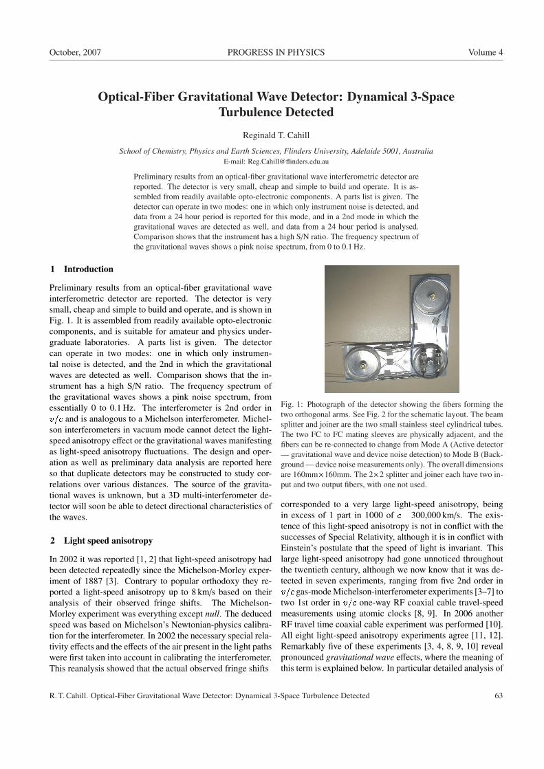
October, 2007 PROGRESS IN PHYSICS Volume 4
Optical-Fiber Gravitational Wave Detector: Dynamical 3-SpaceTurbulence Detected
Reginald T. Cahill
School of Chemistry, Physics and Earth Sciences, Flinders University, Adelaide 5001, AustraliaE-mail: [email protected]
Preliminary results from an optical-fiber gravitational wave interferometric detector arereported. The detector is very small, cheap and simple to build and operate. It is as-sembled from readily available opto-electronic components. A parts list is given. Thedetector can operate in two modes: one in which only instrument noise is detected, anddata from a 24 hour period is reported for this mode, and in a 2nd mode in which thegravitational waves are detected as well, and data from a 24 hour period is analysed.Comparison shows that the instrument has a high S/N ratio. The frequency spectrum ofthe gravitational waves shows a pink noise spectrum, from 0 to 0.1 Hz.
1 Introduction
Preliminary results from an optical-fiber gravitational waveinterferometric detector are reported. The detector is verysmall, cheap and simple to build and operate, and is shown inFig. 1. It is assembled from readily available opto-electroniccomponents, and is suitable for amateur and physics under-graduate laboratories. A parts list is given. The detectorcan operate in two modes: one in which only instrumen-tal noise is detected, and the 2nd in which the gravitationalwaves are detected as well. Comparison shows that the in-strument has a high S/N ratio. The frequency spectrum ofthe gravitational waves shows a pink noise spectrum, fromessentially 0 to 0.1 Hz. The interferometer is 2nd order inv=c and is analogous to a Michelson interferometer. Michel-son interferometers in vacuum mode cannot detect the light-speed anisotropy effect or the gravitational waves manifestingas light-speed anisotropy fluctuations. The design and oper-ation as well as preliminary data analysis are reported hereso that duplicate detectors may be constructed to study cor-relations over various distances. The source of the gravita-tional waves is unknown, but a 3D multi-interferometer de-tector will soon be able to detect directional characteristics ofthe waves.
2 Light speed anisotropy
In 2002 it was reported [1, 2] that light-speed anisotropy hadbeen detected repeatedly since the Michelson-Morley exper-iment of 1887 [3]. Contrary to popular orthodoxy they re-ported a light-speed anisotropy up to 8 km/s based on theiranalysis of their observed fringe shifts. The Michelson-Morley experiment was everything except null. The deducedspeed was based on Michelson’s Newtonian-physics calibra-tion for the interferometer. In 2002 the necessary special rela-tivity effects and the effects of the air present in the light pathswere first taken into account in calibrating the interferometer.This reanalysis showed that the actual observed fringe shifts
Fig. 1: Photograph of the detector showing the fibers forming thetwo orthogonal arms. See Fig. 2 for the schematic layout. The beamsplitter and joiner are the two small stainless steel cylindrical tubes.The two FC to FC mating sleeves are physically adjacent, and thefibers can be re-connected to change from Mode A (Active detector— gravitational wave and device noise detection) to Mode B (Back-ground — device noise measurements only). The overall dimensionsare 160mm�160mm. The 2�2 splitter and joiner each have two in-put and two output fibers, with one not used.
corresponded to a very large light-speed anisotropy, beingin excess of 1 part in 1000 of c= 300,000 km/s. The exis-tence of this light-speed anisotropy is not in conflict with thesuccesses of Special Relativity, although it is in conflict withEinstein’s postulate that the speed of light is invariant. Thislarge light-speed anisotropy had gone unnoticed throughoutthe twentieth century, although we now know that it was de-tected in seven experiments, ranging from five 2nd order inv=c gas-mode Michelson-interferometer experiments [3–7] totwo 1st order in v=c one-way RF coaxial cable travel-speedmeasurements using atomic clocks [8, 9]. In 2006 anotherRF travel time coaxial cable experiment was performed [10].All eight light-speed anisotropy experiments agree [11, 12].Remarkably five of these experiments [3, 4, 8, 9, 10] revealpronounced gravitational wave effects, where the meaning ofthis term is explained below. In particular detailed analysis of
R. T. Cahill. Optical-Fiber Gravitational Wave Detector: Dynamical 3-Space Turbulence Detected 63
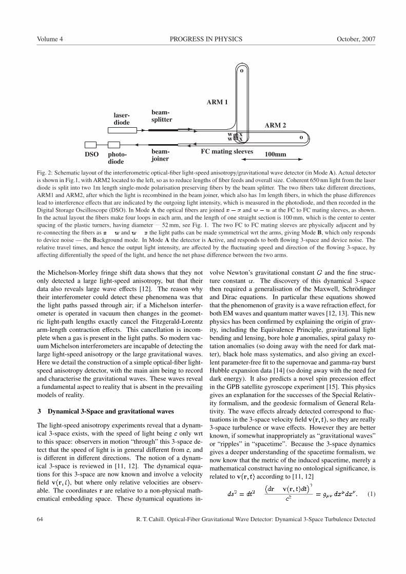
Volume 4 PROGRESS IN PHYSICS October, 2007
laser-diode
beam-splitter
-
photo-diode
DSO beam-joiner
¾
¸
¶³
°±
²©
°
-- ³ª±
² ³´¾¾
FC mating sleeves
ARM 1
ARM 2
-¾ 100mm
o
o
xx
ww
Fig. 2: Schematic layout of the interferometric optical-fiber light-speed anisotropy/gravitational wave detector (in Mode A). Actual detectoris shown in Fig.1, with ARM2 located to the left, so as to reduce lengths of fiber feeds and overall size. Coherent 650 nm light from the laserdiode is split into two 1m length single-mode polarisation preserving fibers by the beam splitter. The two fibers take different directions,ARM1 and ARM2, after which the light is recombined in the beam joiner, which also has 1m length fibers, in which the phase differenceslead to interference effects that are indicated by the outgoing light intensity, which is measured in the photodiode, and then recorded in theDigital Storage Oscilloscope (DSO). In Mode A the optical fibers are joined x � x and w � w at the FC to FC mating sleeves, as shown.In the actual layout the fibers make four loops in each arm, and the length of one straight section is 100 mm, which is the center to centerspacing of the plastic turners, having diameter = 52 mm, see Fig. 1. The two FC to FC mating sleeves are physically adjacent and byre-connecting the fibers as x � w and w � x the light paths can be made symmetrical wrt the arms, giving Mode B, which only respondsto device noise — the Background mode. In Mode A the detector is Active, and responds to both flowing 3-space and device noise. Therelative travel times, and hence the output light intensity, are affected by the fluctuating speed and direction of the flowing 3-space, byaffecting differentially the speed of the light, and hence the net phase difference between the two arms.
the Michelson-Morley fringe shift data shows that they notonly detected a large light-speed anisotropy, but that theirdata also reveals large wave effects [12]. The reason whytheir interferometer could detect these phenomena was thatthe light paths passed through air; if a Michelson interfer-ometer is operated in vacuum then changes in the geomet-ric light-path lengths exactly cancel the Fitzgerald-Lorentzarm-length contraction effects. This cancellation is incom-plete when a gas is present in the light paths. So modern vac-uum Michelson interferometers are incapable of detecting thelarge light-speed anisotropy or the large gravitational waves.Here we detail the construction of a simple optical-fiber light-speed anisotropy detector, with the main aim being to recordand characterise the gravitational waves. These waves reveala fundamental aspect to reality that is absent in the prevailingmodels of reality.
3 Dynamical 3-Space and gravitational waves
The light-speed anisotropy experiments reveal that a dynam-ical 3-space exists, with the speed of light being c only wrtto this space: observers in motion “through” this 3-space de-tect that the speed of light is in general different from c, andis different in different directions. The notion of a dynam-ical 3-space is reviewed in [11, 12]. The dynamical equa-tions for this 3-space are now known and involve a velocityfield v(r; t), but where only relative velocities are observ-able. The coordinates r are relative to a non-physical math-ematical embedding space. These dynamical equations in-
volve Newton’s gravitational constant G and the fine struc-ture constant �. The discovery of this dynamical 3-spacethen required a generalisation of the Maxwell, Schrodingerand Dirac equations. In particular these equations showedthat the phenomenon of gravity is a wave refraction effect, forboth EM waves and quantum matter waves [12, 13]. This newphysics has been confirmed by explaining the origin of grav-ity, including the Equivalence Principle, gravitational lightbending and lensing, bore hole g anomalies, spiral galaxy ro-tation anomalies (so doing away with the need for dark mat-ter), black hole mass systematics, and also giving an excel-lent parameter-free fit to the supernovae and gamma-ray burstHubble expansion data [14] (so doing away with the need fordark energy). It also predicts a novel spin precession effectin the GPB satellite gyroscope experiment [15]. This physicsgives an explanation for the successes of the Special Relativ-ity formalism, and the geodesic formalism of General Rela-tivity. The wave effects already detected correspond to fluc-tuations in the 3-space velocity field v(r; t), so they are really3-space turbulence or wave effects. However they are betterknown, if somewhat inappropriately as “gravitational waves”or “ripples” in “spacetime”. Because the 3-space dynamicsgives a deeper understanding of the spacetime formalism, wenow know that the metric of the induced spacetime, merely amathematical construct having no ontological significance, isrelated to v(r; t) according to [11, 12]
ds2 = dt2 ��dr� v(r; t)dt
�2c2
= g�� dx�dx� : (1)
64 R. T. Cahill. Optical-Fiber Gravitational Wave Detector: Dynamical 3-Space Turbulence Detected
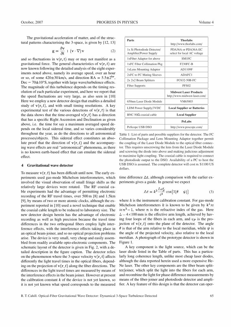
October, 2007 PROGRESS IN PHYSICS Volume 4
The gravitational acceleration of matter, and of the struc-tural patterns characterising the 3-space, is given by [12, 13]
g =@v@t
+ (v � r)v (2)
and so fluctuations in v(r; t) may or may not manifest as agravitational force. The general characteristics of v(r; t) arenow known following the detailed analysis of the eight exper-iments noted above, namely its average speed, over an houror so, of some 420�30 km/s, and direction RA = 5.5�2hr,Dec = 70�10�S, together with large wave/turbulence effects.The magnitude of this turbulence depends on the timing res-olution of each particular experiment, and here we report thatthe speed fluctuations are very large, as also seen in [10]Here we employ a new detector design that enables a detailedstudy of v(r; t), and with small timing resolutions. A keyexperimental test of the various detections of v(r; t) is thatthe data shows that the time-averaged v(r; t) has a directionthat has a specific Right Ascension and Declination as givenabove, i.e. the time for say a maximum averaged speed de-pends on the local sidereal time, and so varies considerablythroughout the year, as do the directions to all astronomicalprocesses/objects. This sidereal effect constitutes an abso-lute proof that the direction of v(r; t) and the accompany-ing wave effects are real “astronomical” phenomena, as thereis no known earth-based effect that can emulate the siderealeffect.
4 Gravitational wave detector
To measure v(r; t) has been difficult until now. The early ex-periments used gas-mode Michelson interferometers, whichinvolved the visual observation of small fringe shifts as therelatively large devices were rotated. The RF coaxial ca-ble experiments had the advantage of permitting electronicrecording of the RF travel times, over 500 m [8] and 1.5km[9], by means of two or more atomic clocks, although the ex-periment reported in [10] used a novel technique that enablethe coaxial cable length to be reduced to laboratory size. Thenew detector design herein has the advantage of electronicrecording as well as high precision because the travel timedifferences in the two orthogonal fibers employ light inter-ference effects, with the interference effects taking place inan optical beam-joiner, and so no optical projection problemsarise. The device is very small, very cheap and easily assem-bled from readily available opto-electronic components. Theschematic layout of the detector is given in Fig. 2, with a de-tailed description in the figure caption. The detector relieson the phenomenon where the 3-space velocity v(r; t) affectsdifferently the light travel times in the optical fibers, depend-ing on the projection of v(r; t) along the fiber directions. Thedifferences in the light travel times are measured by means ofthe interference effects in the beam joiner. However at presentthe calibration constant k of the device is not yet known, soit is not yet known what speed corresponds to the measured
Parts Thorlabshttp://www.thorlabs.com/
1x Si Photodiode Detector/ PDA36A or PDA36A-ECAmplifier/Power Supply select for local AC voltage
1xFiber Adaptor for above SM1FC
1xFC Fiber Collimation Pkg F230FC-B
1xLens Mounting Adaptor AD1109F
2xFC to FC Mating Sleeves ADAFC1
2x 2x2 Beam Splitters FC632-50B-FC
Fiber Supports PFS02
Midwest Laser Productshttp://www.midwest-laser.com/
650nm Laser Diode Module VM65003
LDM Power Supply/3VDC Local Supplier or Batteries
BNC 50 coaxial cable Local Supplier
PoLabs
PoScope USB DSO http://www.poscope.com/
Table 1: List of parts and possible suppliers for the detector. The FCCollimation Package and Lens Mounting Adaptor together permitthe coupling of the Laser Diode Module to the optical fiber connec-tor. This requires unscrewing the lens from the Laser Diode Moduleand screwing the diode into above and making judicious adjustmentto maximise light coupling. The coaxial cable is required to connectthe photodiode output to the DSO. Availability of a PC to host theUSB DSO is assumed. The complete detector will cost � $1100 USdollars.
time difference �t, although comparison with the earlier ex-periments gives a guide. In general we expect
�t = k2Lv2P
c3cos�2(� � )
�(3)
where k is the instrument calibration constant. For gas-modeMichelson interferometers k is known to be given by k2��n2� 1, where n is the refractive index of the gas. HereL= 4�100 mm is the effective arm length, achieved by hav-ing four loops of the fibers in each arm, and vP is the pro-jection of v(r; t) onto the plane of the detector. The angle� is that of the arm relative to the local meridian, while isthe angle of the projected velocity, also relative to the localmeridian. A photograph of the prototype detector is shown inFigure 1.
A key component is the light source, which can be thelaser diode listed in the Table of parts. This has a particu-larly long coherence length, unlike most cheap laser diodes,although the data reported herein used a more expensive He-Ne laser. The other key components are the fiber beam split-ter/joiner, which split the light into the fibers for each arm,and recombine the light for phase difference measurements bymeans of the fiber-joiner and photodiode detector and ampli-fier. A key feature of this design is that the detector can oper-
R. T. Cahill. Optical-Fiber Gravitational Wave Detector: Dynamical 3-Space Turbulence Detected 65
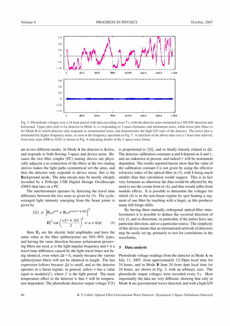
Volume 4 PROGRESS IN PHYSICS October, 2007
Fig. 3: Photodiode voltages over a 24 hour period with data recording every 5 s, with the detector arms orientated in a NS-EW direction andhorizontal. Upper plot (red) is for detector in Mode A, i.e responding to 3-space dynamics and instrument noise, while lower plot (blue) isfor Mode B in which detector only responds to instrumental noise, and demonstrates the high S/N ratio of the detector. The lower plot isdominated by higher frequency noise, as seen in the frequency spectrum in Fig. 5. A selection of the above data over a 1 hour time interval,from time steps 4900 to 5620, is shown in Fig. 4 indicating details of the 3-space wave forms.
ate in two different modes. In Mode A the detector is Active,and responds to both flowing 3-space and device noise. Be-cause the two fiber coupler (FC) mating sleeves are physi-cally adjacent a re-connection of the fibers at the two matingsleeves makes the light paths symmetrical wrt the arms, andthen the detector only responds to device noise; this is theBackground mode. The data stream may be mostly cheaplyrecorded by a PoScope USB Digital Storage Oscilloscope(DSO) that runs on a PC.
The interferometer operates by detecting the travel timedifference between the two arms as given by (3). The cycle-averaged light intensity emerging from the beam joiner isgiven by
I(t) /���E1 ei!t + E2 ei!(t+�+�t)
���2= jEj2 cos
�!(� + �t)
2
�2� a+ b�t : (4)
Here Ei are the electric field amplitudes and have thesame value as the fiber splitter/joiner are 50%-50% types,and having the same direction because polarisation preserv-ing fibers are used, ! is the light angular frequency and � is atravel time difference caused by the light travel times not be-ing identical, even when �t= 0, mainly because the varioussplitter/joiner fibers will not be identical in length. The lastexpression follows because �t is small, and so the detectoroperates in a linear regime, in general, unless � has a valueequal to modulo(T ), where T is the light period. The maintemperature effect in the detector is that � will be tempera-ture dependent. The photodiode detector output voltage V (t)
is proportional to I(t), and so finally linearly related to �t.The detector calibration constants a and b depend on k and � ,and are unknown at present, and indeed � will be instrumentdependent. The results reported herein show that the value ofthe calibration constant b is not given by using the effectiverefractive index of the optical fiber in (3), with b being muchsmaller than that calculation would suggest. This is in factvery fortunate as otherwise the data would be affected by theneed to use the cosine form in (4), and thus would suffer frommodulo effects. It is possible to determine the voltages forwhich (4) is in the non-linear regime by spot heating a seg-ment of one fiber by touching with a finger, as this producesmany full fringe shifts.
By having three mutually orthogonal optical-fiber inter-ferometers it is possible to deduce the vectorial direction ofv(r; t), and so determine, in particular, if the pulses have anyparticular direction, and so a particular source. The simplicityof this device means that an international network of detectorsmay be easily set up, primarily to test for correlations in thewaveforms.
5 Data analysis
Photodiode voltage readings from the detector in Mode A onJuly 11, 2007, from approximately 12:30pm local time for24 hours, and in Mode B June 24 from 4pm local time for24 hours, are shown in Fig. 3, with an arbitrary zero. Thephotodiode output voltages were recorded every 5 s. Mostimportantly the data are very different, showing that only inMode A are gravitational waves detected, and with a high S/N
66 R. T. Cahill. Optical-Fiber Gravitational Wave Detector: Dynamical 3-Space Turbulence Detected
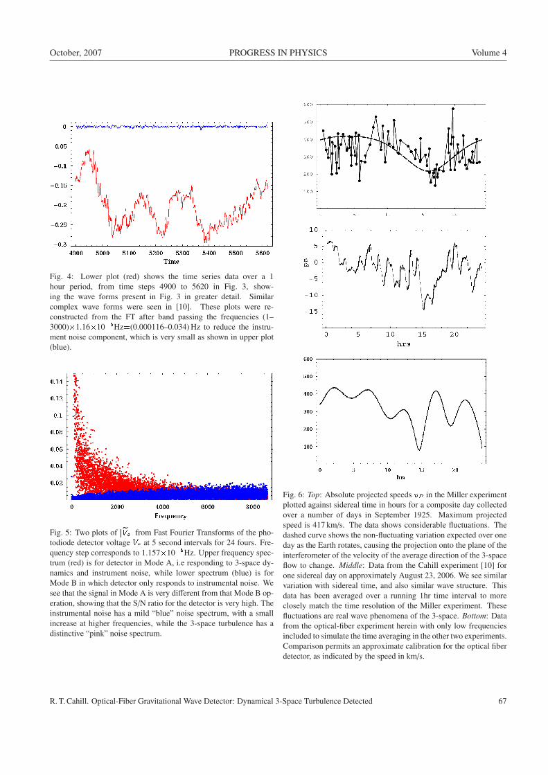
October, 2007 PROGRESS IN PHYSICS Volume 4
Fig. 4: Lower plot (red) shows the time series data over a 1hour period, from time steps 4900 to 5620 in Fig. 3, show-ing the wave forms present in Fig. 3 in greater detail. Similarcomplex wave forms were seen in [10]. These plots were re-constructed from the FT after band passing the frequencies (1–3000)�1.16�10�5Hz=(0.000116–0.034) Hz to reduce the instru-ment noise component, which is very small as shown in upper plot(blue).
Fig. 5: Two plots of jeVsj from Fast Fourier Transforms of the pho-todiode detector voltage Vr at 5 second intervals for 24 fours. Fre-quency step corresponds to 1.157�10�5Hz. Upper frequency spec-trum (red) is for detector in Mode A, i.e responding to 3-space dy-namics and instrument noise, while lower spectrum (blue) is forMode B in which detector only responds to instrumental noise. Wesee that the signal in Mode A is very different from that Mode B op-eration, showing that the S/N ratio for the detector is very high. Theinstrumental noise has a mild “blue” noise spectrum, with a smallincrease at higher frequencies, while the 3-space turbulence has adistinctive “pink” noise spectrum.
Fig. 6: Top: Absolute projected speeds vP in the Miller experimentplotted against sidereal time in hours for a composite day collectedover a number of days in September 1925. Maximum projectedspeed is 417 km/s. The data shows considerable fluctuations. Thedashed curve shows the non-fluctuating variation expected over oneday as the Earth rotates, causing the projection onto the plane of theinterferometer of the velocity of the average direction of the 3-spaceflow to change. Middle: Data from the Cahill experiment [10] forone sidereal day on approximately August 23, 2006. We see similarvariation with sidereal time, and also similar wave structure. Thisdata has been averaged over a running 1hr time interval to moreclosely match the time resolution of the Miller experiment. Thesefluctuations are real wave phenomena of the 3-space. Bottom: Datafrom the optical-fiber experiment herein with only low frequenciesincluded to simulate the time averaging in the other two experiments.Comparison permits an approximate calibration for the optical fiberdetector, as indicated by the speed in km/s.
R. T. Cahill. Optical-Fiber Gravitational Wave Detector: Dynamical 3-Space Turbulence Detected 67

Volume 4 PROGRESS IN PHYSICS October, 2007
ratio. A 1 hour time segment of that data is shown in Fig. 4.In that plot the higher frequencies have been filtered out fromboth data time series, showing the exceptional S/N ratio thatcan be achieved.
In Fig. 5 the Fourier Transfoms of the two data time seriesare shown, again revealing the very different characteristicsof the data from the two operating modes. The instrumentalnoise has a mild “blue” noise spectrum, with a small increaseat higher frequencies, while the 3-space turbulence has a dis-tinctive “pink” noise spectrum, and ranging essentially from0 to 0.1 Hz. The FT is defined by
eVs =1pn
nXr=1
Vre2�i(r�1)(s�1)=n (5)
where n= 17280 corresponds to a 5 s timing interval over 24hours.
By removing all but the FT amplitudes 1–10, and theninverse Fourier Transforming we obtain the slow changes oc-curring over 24 hours. The resulting data has been presentedin terms of possible values for the projected speed vP in (3),and is shown in Fig. 6 and plotted against sidereal time, afteradjusting the unknown calibration constants to give a formresembling the Miller and coaxial cable experimental resultsso as to give some indication of the calibration of the detec-tor. The experiment was run in an unoccupied office in whichtemperatures varied by some 10�C over the 24 hour periods.In future temperature control will be introduced.
6 Conclusions
As reviewed in [11, 12] gravitational waves, that is, fluc-tuations or turbulence in the dynamical 3-space, have beendetected since the 1887 Michelson-Morley experiment, al-though this all went unrealised until recently. As the timingresolution improved over the century, from initially one hourto seconds now, the characteristics of the turbulence of thedynamical 3-space have become more apparent, and that atsmaller timing resolutions the turbulence is seen to be verylarge. As shown herein this wave/pulse phenomenon is veryeasy to detect, and opens up a whole new window on the uni-verse. The detector reported here took measurements every5 s, but can be run at millisecond acquisition rates. A 3Dversion of the detector with three orthogonal optical-fiber in-terferometers will soon become operational. This will permitthe determination of the directional characteristics of the 3-space pulses.
That the average 3-space flow will affect the gyroscopeprecessions in the GP-B satellite experiment through vortic-ity effects was reported in [15]. The fluctuations are also pre-dicted to be detectable in that experiment as noted in [16].However the much larger fluctuations detected in [10] andherein imply that these effects will be much large than re-ported in [16] where the time averaged waves from the De-
Witte experiment [9] were used; essentially the gyro preces-sions will appear to have a large stochasticity.
Special thanks to Peter Morris, Thomas Goodey, Tim East-man, Finn Stokes and Dmitri Rabounski.
Submitted on July 09, 2007Accepted on July 16, 2007
References
1. Cahill R.T. and Kitto K. Michelson-Morley experiments revis-ited. Apeiron, 2003, v. 10(2),104–117.
2. Cahill R.T. The Michelson and Morley 1887 experiment andthe discovery of absolute motion. Progress in Physics, 2005,v. 3, 25–29.
3. Michelson A. A. and Morley E. W. Philos. Mag., 1887, S. 5, 24,No. 151, 449–463.
4. Miller D. C. Rev. Mod. Phys., 1933, v. 5, 203–242.
5. Illingworth K. K. Phys. Rev., 1927, v. 3, 692–696.
6. Joos G. Ann. d. Physik, 1930, v. 7, 385.
7. Jaseja T. S. et al. Phys. Rev. A, 1964, v. 133, 1221.
8. Torr D. G. and Kolen P. In: Precision Measurements and Fun-damental Constants, Taylor, B. N. and Phillips, W. D. eds.,Natl. Bur. Stand. (U.S.), Spec. Publ., 1984, v. 617, 675.
9. Cahill R. T. The Roland DeWitte 1991 experiment. Progress inPhysics, 2006, v. 3, 60–65.
10. Cahill R. T. A new light-speed anisotropy experiment: absolutemotion and gravitational waves detected. Progress in Physics,2006, v. 4, 73–92.
11. Cahill R. T. Process physics: from information theory to quan-tum space and matter. Nova Science Pub., New York, 2005.
12. Cahill R. T. Dynamical 3-space: a review. arXiv: 0705.4146.
13. Cahill R. T. Dynamical fractal 3-space and the generalisedSchrodinger equation: equivalence principle and vorticity ef-fects. Progress in Physics, 2006, v. 1, 27–34.
14. Cahill R. T. Dynamical 3-space: supernovae and the Hubbleexpansion — the older Universe without Dark Energy. Progressin Physics, 2007, v. 4, 9–12.
15. Cahill R. T. Novel Gravity Probe B frame-dragging effect.Progress in Physics, 2005, v. 3, 30–33.
16. Cahill R. T. Novel Gravity Probe B gravitational wave detec-tion. arXiv: physics/0407133.
68 R. T. Cahill. Optical-Fiber Gravitational Wave Detector: Dynamical 3-Space Turbulence Detected
October, 2007 PROGRESS IN PHYSICS Volume 4
On the “Size” of Einstein’s Spherically Symmetric Universe
Stephen J. CrothersQueensland, Australia
E-mail: [email protected]
It is alleged by the Standard Cosmological Model that Einstein’s Universe is finite butunbounded. Although this is a longstanding and widespread allegation, it is nonethelessincorrect. It is also alleged by this Model that the Universe is expanding and that itbegan with a Big Bang. These are also longstanding and widespread claims that aredemonstrably false. The FRW models for an expanding, finite, unbounded Universe areinconsistent with General Relativity and are therefore invalid.
1 Historical basis
Non-static homogeneous models were first investigated theo-retically by Friedmann in 1922. The concept of the Big Bangbegan with Lemaıtre, in 1927, who subsequently asserted thatthe Universe, according to General Relativity, came into ex-istence from a “primaeval atom”.
Following Friedmann, the work of Robertson andWalker resulted in the FRW line-element,
ds2 = dt2 �R2(t)�
dr2
1� kr2 + r2 �d�2 + sin2� d'2�� ;from which is obtained the so-called “Friedmann equation”,
_R2 + k =8�G
3�R2;
where � is the macroscopic proper density of the Universe andk a constant. Applying the continuity condition T�� ;� = 0,to the stress tensor T�� of a perfect fluid
T�� = (�+ p)u�u� � pg�� ;where p is the pressure and u� the covariant world velocityof the fluid particles, the equation of continuity becomes
R _�+ 3 _R(�+ p) = 0 :
With the ad hoc assumption thatR(0) = 0, the Friedmannequation is routinely written as
_R2 + k =A2
R;
where A is a constant. The so-called “Friedmann models”are:
(1) k = 0 — the flat model,(2) k = 1 — the closed model,(3) k = �1 — the open model,
wherein t = 0 is claimed to mark the beginning of the Uni-verse and R(0) = 0 the cosmological singularity.
Big Bang and expansion now dominate thinking in con-temporary cosmology. However, it is nonetheless easily prov-
ed that such cosmological models, insofar as they relate tothe FRW line-element, with or without embellishments suchas “inflation”, are in fact inconsistent with the mathematicalstructure of the line-elements from which they are alleged,and are therefore false.
2 Spherically symmetric metric manifolds
A 3-D spherically symmetric metric manifold has, in thespherical-polar coordinates, the following form ([1, 2]),
ds2 = B(Rc)dR2c +R2
c(d�2 + sin2� d'2) ; (1)
where B(Rc) and Rc = Rc(r) are a priori unknown analyticfunctions of the variable r of the simple line element
ds2 = dr2 + r2(d�2 + sin2� d'2) ; (2)
0 6 r 61 :
Line elements (1) and (2) have precisely the same fun-damental geometric form and so the geometric relations be-tween the components of the metric tensor are exactly thesame in each line element. The quantity Rc appearing in (1)is not the geodesic radial distance associated with the mani-fold it describes. It is in fact the radius of curvature, in thatit determines the Gaussian curvature G = 1=R2
c (see [1, 2]).The geodesic radial distance distance, Rp, from an arbitrarypoint in the manifold described by (1) is an intrinsic geomet-ric property of the line element, and is given by
Rp =Z p
B(Rc) dRc + C =Z p
B(Rc)dRcdr
dr + C ;
where C is a constant of integration to be determined ([2]).Therefore, (1) can be written as
ds2 = dR2p +R2
c(d�2 + sin2� d'2) ;
wheredRp =
pB(Rc) dRc ;
and0 6 Rp <1 ;
S. J. Crothers. On the “Size” of Einstein’s Universe 69
Volume 4 PROGRESS IN PHYSICS October, 2007
with the possibility of the line element being singular (unde-fined) at Rp = 0, since B(Rc) and Rc = Rc(r) are a pri-ori unknown analytic functions of the variable r. In the caseof (2),
Rc(r) � r; dRp � dr; B(Rc(r)) � 1 ;
from which it follows that Rc � Rp � r in the case of (2).Thus Rc � Rp is not general, and only occurs in the specialcase of (2), which describes an Efcleethean� space.
The volume V of (1), and therefore of (2), is
V =Z Rp
0R2c dRp
Z �
0sin � d�
Z 2�
0d' =
= 4�Z Rc(r)
Rc(0)R2c(r)
pB(Rc(r)) dRc(r) =
= 4�Z r
0R2c(r)
pB(Rc(r))
dRc(r)dr
dr ;
although, in the general case (1), owing to the a priori un-known functions B(Rc(r)) and Rc(r), the line element (1)may be undefined at Rp(Rc(0)) = Rp(r = 0) = 0, which isthe location of the centre of spherical symmetry of the man-ifold of (1) at an arbitrary point in the manifold. Also, sinceRc(r) is a priori unknown, the value of Rc(0) is unknownand so it cannot be assumed that Rc(0) = 0. In the specialcase of (2), both B(Rc(r)) and Rc(r) are known.
Similarly, the surface area S of (1), and hence of (2), isgiven by the general expression,
S = R2c(r)
Z �
0sin � d�
Z 2�
0d' = 4�R2
c(r) :
This might not ever be zero, since, once again, Rc(r) is an apriori unknown function and so Rc(0) might not be zero. Itall depends an the explicit form for Rc(r), if it can be deter-mined in a given situation, and on associated boundary con-ditions. References [1, 2] herein describe the mathematics inmore detail.
3 The “radius” of Einstein’s universe
Since a geometry is entirely determined by the form of itsline element [3], everything must be determined from it. Onecannot, as is usually done, merely foist assumptions upon it.The intrinsic geometry of the line element and the consequentgeometrical relations between the components of the metrictensor determine all.
Consider the usual non-static cosmological line element
ds2 = dt2 � eg(t)�1+k
4 �r2�2 �d�r2+�r2(d�2+ sin2� d'2)
�; (3)
wherein it is usually simply assumed that 0 6 �r <1 [3–6].�For the geometry due to Efcleethees, usually and abominably rendered
as Euclid.
However, the range on �r must be determined, not assumed. Itis easily proved that the foregoing usual assumption is patent-ly false.
Once again note that in (3) the quantity �r is not a radialgeodesic distance. In fact, it is not even a radius of curvatureon (3). It is merely a parameter for the radius of curvatureand the proper radius, both of which are well-defined by theform of the line element (describing a spherically symmetricmetric manifold). The radius of curvature, Rc, for (3), is
Rc = e12 g(t)
�r1 + k
4 �r2: (4)
The proper radius for (3) is given by
Rp = e12 g(t)
Zd�r
1 + k4 �r2
=
=2e 1
2 g(t)pk
arctan
pk
2�r + n�
!; n = 0; 1; 2; : : :
(5)
Since Rp > 0 by definition, Rp = 0 is satisfied when �r== 0 =n. So �r= 0 is the lower bound on �r. The upper boundon �r must now be ascertained from the line element andboundary conditions.
It is noted that the spatial component of (4) has a maxi-mum of 1p
kfor any time t, when �r= 2p
k. Thus, as �r ! 1,
the spatial component ofRc runs from 0 (at �r= 0) to the max-imum 1p
k(at �r= 2p
k), then back to zero, since
lim�r!1
�r1 + k
4 �r2= 0: (6)
Transform (3) by setting
R = R(�r) =�r
1 + k4 �r2
; (7)
which carries (3) into
ds2 = dt2�eg(t)�
dR2
1� kR2 +R2(d�2 + sin2� d'2)�: (8)
The quantity R appearing in (8) is not a radialgeodesic distance. It is only a factor in a radius of curva-ture in that it determines the Gaussian curvatureG = 1
eg(t)R2 .The radius of curvature of (8) is
Rc = e12 g(t)R; (9)
and the proper radius of Einstein’s universe is, by (8),
Rp = e12 g(t)
ZdRp
1� kR2=
=e 1
2 g(t)pk
�arcsin
pkR+ 2m�
�; m = 0; 1; 2; : : :
(10)
Now according to (7), the minimum value of R isR (�r= 0) = 0. Also, according to (7), the maximum value
70 S. J. Crothers. On the “Size” of Einstein’s Universe

October, 2007 PROGRESS IN PHYSICS Volume 4
of R is R(�r= 2pk) = 1p
k. R= 1p
kmakes (8) singular, al-
though (3) is not singular at �r= 2pk
. Since by (7), �r !1)R(�r)! 0, then if 06 �r <1 on (3) it follows that the properradius of Einstein’s universe is, according to (8),
Rp = e12 g(t)
Z 0
0
dRp1� kR2
� 0 : (11)
Therefore, 06 �r <1 on (3) is false. Furthermore, sincethe proper radius of Einstein’s universe cannot be zero andcannot depend upon a set of coordinates (it must be an in-variant), expressions (5) and (10) must agree. Similarly, theradius of curvature of Einstein’s universe must be an invariant(independent of a set of coordinates), so expressions (4) and(9) must also agree, in which case 06R< 1p
kand 06�r< 2p
k.
Then by (5), the proper radius of Einstein’s universe is
Rp = lim�! 2p
k
e12 g(t)
Z �
0
d�r1 + k
4 �r2=
=2e 1
2 g(t)pk
h��4
+ n���m�i ; n;m = 0; 1; 2; : : :
n > m:
Setting p = n�m gives for the proper radius of Einstein’suniverse,
Rp =2e 1
2 g(t)pk
��4
+ p��; p = 0; 1; 2; : : : (12)
Now by (10), the proper radius of Einstein’s universe is
Rp = lim�! 1p
k
e12 g(t)
Z �
0
dRp1� kR2
=
=e 1
2 g(t)pk
h��2
+ 2n���m�i ; n;m = 0; 1; 2; : : :
2n > m:
Setting q = 2n�m gives the proper radius of Einstein’suniverse as,
Rp =e 1
2 g(t)pk
��2
+ q��; q = 0; 1; 2; : : : (13)
Expressions (12) and (13) must be equal for all valuesof p and q. This can only occur if g(t) is infinite for allvalues of t. Thus, the proper radius of Einstein’s universeis infinite.
By (4), (7) and (9), the invariant radius of curvature ofEinstein’s universe is,
Rc
�2pk
�=e 1
2 g(t)pk; (14)
which is infinite by virtue of g(t) =1 8 t.
4 The “volume” of Einstein’s universe
The volume of Einstein’s universe is, according to (3),
V = e32 g(t)
Z 2pk
0
�r2d�r�1 + k
4 �r2�3 Z �
0sin �d�
Z 2�
0d' =
=4�e 3
2 g(t)
k 32
��4
+ p��; p = 0; 1; 2; : : :
(15)
The volume of Einstein’s universe is, according to (8),
V = e32 g(t)
Z 1pk
0
R2dRp1� kR2
Z �
0sin �d�
Z 2�
0d' =
= e32 g(t)
2�k 3
2
h�2
+ (2n�m)�i; n;m = 0; 1; 2; : : :
2n > m;
and setting q = 2n�m this becomes,
V =2�e 3
2 g(t)
k 32
��2
+ q��; q = 0; 1; 2; : : : (16)
Since the volume of Einstein’s universe must be an invari-ant, expressions (15) and (16) must be equal for all values ofp and q. Equality can only occur if g(t) is infinite for all val-ues of the time t. Thus the volume of Einstein’s universe isinfinite.
In the usual treatment (8) is transformed by setting
R =1pk
sin�; (17)
to get
ds2 = dt2 � eg(t)
k�d�2 + sin2�(d�2 + sin2� d'2)
�; (18)
where it is usually asserted, without any proof (see e.g. [3, 4,5, 6]), that
0 6 � 6 � (or 0 6 � 6 2�); (19)
and whereby (18) is not singular. However, according to (7),(11), (12), and (13), � can only take the values
2n� 6 � <�2
+ 2n�; n = 0; 1; 2; : : :
so that the radius of curvature of Einstein’s universe is,by (18),
Rc =e 1
2 g(t) sin�pk
which must be evaluated for � = �2 + 2n�, n = 0; 1; 2; : : :,
giving
Rc =e 1
2 g(t)pk
as the radius of curvature of Einstein’s universe, in concor-dance with (4), (7), and (9). The proper radius of Einstein’s
S. J. Crothers. On the “Size” of Einstein’s Universe 71
Volume 4 PROGRESS IN PHYSICS October, 2007
universe is given by
Rp =e 1
2 g(t)pk
Z �2 +2n�
2n�d� =
e 12 g(t)pk�2; (20)
and since the proper radius of Einstein’s universe is an invari-ant, (20) must equal (12) and (13). Expression (20) is consis-tent with (12) and (13) only if g(t) is infinite for all values ofthe time t, and so Einstein’s universe is infinite.
According to (18), the volume of Einstein’s universe is,
V =e 3
2 g(t)
k 32
Z �2 +2n�
2n�sin2� d�
Z �
0sin �d�
Z 2�
0d' =
=�2e 3
2 g(t)
k 32
�2:
(21)
Since this volume must be an invariant, expression (21)must give the same value as expressions (15) and (16). Thiscan only occur for (21) if g(t) is infinite for all values of thetime t, and so Einstein’s universe has an infinite volume.
5 The “area” of Einstein’s universe
Using (3), the invariant surface area of Einstein’s universe is
S = R2c
Z �
0sin �d�
Z 2�
0d' = 4�R2
c
which must be evaluated for Rc(�r = 2pk), according to (4),
and so
S =4�eg(t)
k:
By (8) the invariant surface area is
S = eg(t)R2Z �
0sin �d�
Z 2�
0d' = 4�R2eg(t);
which must, according to (7), be evaluated forR(�r = 2p
k) = 1p
k, to give
S =4�eg(t)
k:
By (18) the invariant surface area is
S =eg(t)
ksin2�
Z �
0sin �d�
Z 2�
0d' =
4�eg(t)
ksin2� ;
and this, according to (17), must be evaluated for �==��
2 + 2n��, n = 0; 1; 2; : : :, which gives
S =4�eg(t)
k:
Thus the invariant surface area of Einstein’s universe isinfinite for all values of the time t, since g(t) is infinite for allvalues of t.
In similar fashion the invariant great “circumference”,C = 2�Rc, of Einstein’s universe is infinite at any particulartime, given by
C =2�e 1
2 g(t)pk
:
6 Generalisation of the line element
Line elements (3), (8) and (18) can be generalised in the fol-lowing way. In (3), replace �r by j�r � �r0j to get
ds2 = dt2 � eg(t)�1 + k
4 j�r � �r0j2�2 �� �d�r2 + j�r � �r0j2(d�2 + sin2� d'2)
�;
(22)
where �r0 2 < is entirely arbitrary. Line element (22) isdefined on
0 6 j�r � �r0j < 2pk8 �r0 ;
i.e. on�r0 � 2p
k< �r <
2pk
+ �r0 8 �r0 : (23)
This corresponds to 06Rc< 1pk
irrespective of the valueof �r0 , and amplifies the fact that �r is merely a parameter. In-deed, (4) is generalised to
Rc = Rc(�r) =j�r � �r0j
1 + k4 j�r � �r0j2 ;
where (23) applies. Note that �r can approach �r0 from aboveor below. Thus, there is nothing special about �r0 = 0. If�r0 = 0 and �r > 0, then (3) is recovered as a special case, stillsubject of course to the range 0 6 �r < 2p
k.
Expression (7) is generalised thus,
jR�R0j = j�r � �r0j1 + k
4 j�r � �r0j2 ;where R0 is an entirely arbitrary real number, and so (8) be-comes
ds2 = dt2 � eg(t)���
dR2
1� kjR�R0j2 + jR�R0j2(d�2 + sin2� d'2)�;
(24)
whereR0 � 1p
k< R <
1pk
+R0 8 R0 : (25)
Note that R can approach R0 from above or below. Thereis nothing special about R0 = 0. If R0 = 0 and R > 0,then (8) is recovered as a special case, subject of course tothe range 0 6 R < 1p
k.
Similarly, (18) is generalised, according to (24), by set-ting
jR�R0j = 1pk
sin j�� �0j ;
72 S. J. Crothers. On the “Size” of Einstein’s Universe
October, 2007 PROGRESS IN PHYSICS Volume 4
where �0 is an entirely arbitrary real number, and
2n� 6 j�� �0j < �2
+ 2n�; n = 0; 1; 2; : : :
8 �0 2 <:Note that � can approach �0 from above or below. There isnothing special about �0 = 0. If �0 = 0 and � > 0, then (18)is recovered as a special case, subject of course to the range2n� 6 � < �
2 + 2n�, n = 0; 1; 2; : : :The corresponding expressions for the great circumfer-
ence, the surface area, and the volume are easily obtained inlike fashion.
7 Conclusions
Einstein’s universe has an infinite proper radius, an infiniteradius of curvature, an infinite surface area and an infinitevolume at any time. Thus, in relation to the Friedmann-Robertson-Walker line-element and its variations consideredherein, the concept of the Big Bang cosmology is invalid.
Submitted on July 16, 2007Accepted on July 20, 2007
References
1. Levi-Civita T. The absolute differential calculus. Dover Publi-cations Inc., New York, 1977.
2. Crothers S. J., Gravitation on a spherically symmetric metricmanifold. Progress in Physics, 2005, v. 2, 68–74.
3. Tolman R. C. Relativity, thermodynamics and cosmology.Dover Publications Inc., New York, 1987.
4. Landau L., Lifshitz E. The classical theory of fields. Addison-Wesley Publishing Company, Inc., Reading, Massachusettes,1951.
5. d’Inverno R. Introducing Einstein’s relativity. Clarendon Press,Oxford, 1992.
6. Misner C. W., Thorne K. S., and Wheeler J. A. Gravitation.W. H. Freeman and Company, New York, 1973.
S. J. Crothers. On the “Size” of Einstein’s Universe 73
Volume 4 PROGRESS IN PHYSICS October, 2007
On the Nature of the Microwave Background at the Lagrange 2 Point. Part I
Pierre-Marie Robitaille
Dept. of Radiology, The Ohio State University, 130 Means Hall, 1654 Upham Drive, Columbus, Ohio 43210, USAE-mail: [email protected]
In this work, the nature of the microwave background is discussed. It is advanced thatthe 2.725 K monopole signal, first detected by Penzias and Wilson, originates from theEarth and therefore cannot be detected at the Lagrange 2 point (L2). Results obtained bythe COBE, Relikt-1, and WMAP satellites are briefly reviewed. Attention is also placedon the upcoming PLANCK mission, with particular emphasis on the low frequency in-strument (LFI). Since the LFI on PLANCK can operate both in absolute mode and indifference mode, this instrument should be able to unequivocally resolve any questionrelative to the origin of the 2.725 K monopole signal. The monopole will be discoveredto originate from the Earth and not from the Cosmos. This will have implications rela-tive to the overall performance of the PLANCK satellite, in particular, and for the futureof astrophysics, in general.
1 Introduction
In 1965, a thermal signal of unknown origin, which appearedto completely engulf the Earth, irrespective of angle of obser-vation, was first reported to exist at microwave frequencies[1]. Immediately considered of great importance, the strangefinding was rapidly attributed to the universe by Dicke et al.[2] in a communication which preceded the disclosure of theactual measurements by A. A. Penzias and R. W. Wilson [1].The observation became known as the “Cosmic MicrowaveBackground (CMB)” nearly from the instant of discovery [1,2]. For years, it had been predicted that such a signal must ex-ist, if the universe evolved from a Big Bang scenario. With theadvent of the Penzias and Wilson measurement [1], the longsought signature of creation seemed discovered, and cosmol-ogy entered the realm of modern science.
Since that time, the “CMB” has become a cornerstoneof astrophysics [3–6]. The background and its characteris-tic 2.725 K monopole temperature [7, 8], the “relic of the BigBang”, is believed to span the entire known universe. Whilethe “CMB” was initially considered weak, it is now clear thatthe signal was in fact quite powerful, at least when viewedfrom Earth orbit (8). Indeed, few experimental signals of nat-ural origin have surpassed the microwave background in ab-solute signal to noise [8]. For cosmology, the “CMB” is themost important “astrophysical” finding. Experimental confir-mations of its existence and characterization have consumedvast amounts of both financial and human capital. As a result,a more detailed understanding of the microwave backgroundhas emerged.
In addition to its characteristic monopole temperature at2.725 K [8], the background has associated with it a strong(3.5 mK) dipole which is ascribed to the motion of the Earthand the Sun through the local group [9]. This powerful dipole
has been observed not only on Earth, and in Earth orbit [9],but also by instruments located well beyond the Earth, likethe Soviet Relikt-1 [10] and the NASA WMAP [11] satel-lites. Consequently, there can be little question that the dipoleis real, and truly associated with motion through the localgroup.
Beyond the dipole, cosmology has also placed significantemphasis on the multipoles visible at microwave frequencies[12]. Accordingly, the universe has now been characterizedby anisotropy maps, the most famous of which have been re-ported by the COBE [7] and WMAP [11] satellites. Thesemaps reflect very slight differences in microwave power ofthe universe as a function of observational direction.
The recent array of scientific evidence, in support of a mi-crowave background of cosmological origin, appears tremen-dous, and cosmology seems to have evolved into a precisionscience [13–19]. Should the 2.725 K microwave backgroundtruly belong to the universe, there can be little question thatcosmology has joined the company of the established exper-imental disciplines. Yet, these claims remain directly linkedto the validity of the assignment for the “Cosmic MicrowaveBackground”. Indeed, if the “CMB” is reassigned to a differ-ent source, astrophysics will undergo significant transforma-tions.
2 The origin of the microwave background
Recently, the origin of the “CMB” has been brought intoquestion, and the monopole of the microwave background hasbeen formally reassigned to the Earth [20–29]. Such claimsdepend on several factors, as follows:
1. The assignment of a 2.725 K temperature to the Pen-zias and Wilson signal constitutes a violation of Kirch-hoff’s Law of Thermal Emission [30, 31]. The proper
74 P.-M. Robitaille. On the Nature of the Microwave Background at the Lagrange 2 Point. Part I
October, 2007 PROGRESS IN PHYSICS Volume 4
assignment of thermal temperatures requires, accord-ing to Kirchhoff [31], equilibrium with an enclosure[30]. This is a condition which cannot be met by theuniverse. Therefore, the absolute magnitude of the tem-perature should be considered erroneous;
2. The cosmological community, in general, and theCOBE [33] and WMAP [34] teams, in particular, haveadvanced that the Earth can be treated as a �300 Kblackbody. In fact, since the Earth is 75% water cov-ered, this assumption is not justified, based on theknown behavior of sea emissions in the microwave re-gion [26, 35]. The oceans exhibit thermal emission pro-files, which depend on the Nadir angle, and are there-fore not blackbody emitters at �300 K. Indeed, theoceans can produce signals very close to 0 K [26, 35]. Itremains of concern that the signature of the microwavebackground is completely devoid of earthly interfer-ence. Not a single artifact has been reported over theentire frequency range [8] which could be attributed toan earthly signal of oceanic origin. At the same time,it is well established that water is a powerful absorberof microwave radiation. Consequently, it is reasonableto expect that the oceans cannot be microwave silentrelative to this problem;
3. Powerful signals imply proximal sources. When mea-sured from the Earth the monopole of the microwavebackground has a tremendous signal to noise [8]. To re-quire that such extensive power fill the entire universeargues in favor of a nearly infinite power source welloutside anything known to human science. Conversely,if the signal arises from the Earth, it would be expectedto be strong when viewed from Earth [8]. The power-ful nature of the microwave background in Earth orbit[8], and the lack of oceanic contaminating signal couldvery easily be solved, if the Penzias and Wilson signal[1] was generated by the Earth itself [20–29];
4. In the experimental setting, thermal photons, once re-leased, report the temperature of the source which pro-duced them in a manner which is independent of timeelapsed and of subsequent source cooling. Once pho-tons are emitted, they cannot shift their frequencies toaccount for changes at the source. Yet, the Big Bangscenario requires a constant and systematic shifting ofphoton frequencies towards lower temperatures in amanner wherein the cooling of the source is constantlymonitored and reported. This is without experimentalevidence in the laboratory. Experimental photons, onceproduced, can no longer monitor the cooling of thesource. Arguments relative to photon shifting, basedon an expanding universe, are theoretical and are notsupported by laboratory measurements. In consideringstellar red shifts, for instance, it is commonly held thatthe sources themselves are moving away from the ob-
server. Thus, the photons are being shifted as they arebeing produced. In sharp contrast, a microwave back-ground of cosmic origin requires continuous shifting ofphoton frequencies long after emission;
5. The monopole of the microwave background is char-acterized by a thermal profile [8]. It is a well recog-nized observation of physics, that a Lyman process isrequired to produce a group of Lyman lines. Like-wise, a nuclear magnetic resonance process is requiredto obtain an NMR line. Similarly, a thermal processmust occur to produce a thermal line. On Earth, ther-mal emission spectra are generated exclusively in thepresence of matter in the condensed state [30]. The ex-istence of a Planckian line in the microwave requiresa process analogous to that which results in a thermalspectrum from a piece of graphite on Earth [30]. Phys-ics has not provided a known mechanism for the cre-ation of a photon by graphite [30]. As a result, Planck’sequation, unlike all others in physics, remains detachedfrom physical reality [30]. In this regard, it is main-tained [30] that a thermal profile can only be obtainedas the result of the vibration of atomic nuclei withinthe confines of a lattice field (or fleeting lattice fieldin the case of a liquid). Condensed matter, either inthe solid or liquid state, is required. This conditioncannot be met within the framework of Big Bang cos-mology. Universality in blackbody radiation does nothold [30, 31];
6. Measurements performed by the COBE satellite reveala systematic error relative to the measured value of themicrowave background monopole temperature, derivedeither from the monopole or the dipole [26, 27]. Thesemeasurements can be interpreted as implying that stillanother field exists through which the Earth is moving[26, 27];
7. Currently, the “Cosmic Microwave Background” isthought to be continuously immersing the Earth in mi-crowave photons from every conceivable direction inspace. Under this steady state scenario, there can be nomeans for signal attenuation at high frequencies, as hasbeen observed on Earth [28]. This strongly argues thatthe “CMB” cannot be of cosmic origin [28];
8. The “CMB” anisotropy maps reported by the WMAPsatellite display instabilities which are unacceptable,given the need for reproducibility on a cosmologicaltimescale. The results fail to meet accepted standardsfor image quality, based on a variety of criteria [23–25]. These findings demonstrate that the stability ob-served in the monopole at 2.725 K is not translated atthe level of the anisotropy maps, as would be expectedfor a signal of cosmologic origin. This implies thatthe monopole arises from a stable source, while theanisotropies arise from separate unstable sources.
P.-M. Robitaille. On the Nature of the Microwave Background at the Lagrange 2 Point. Part I 75
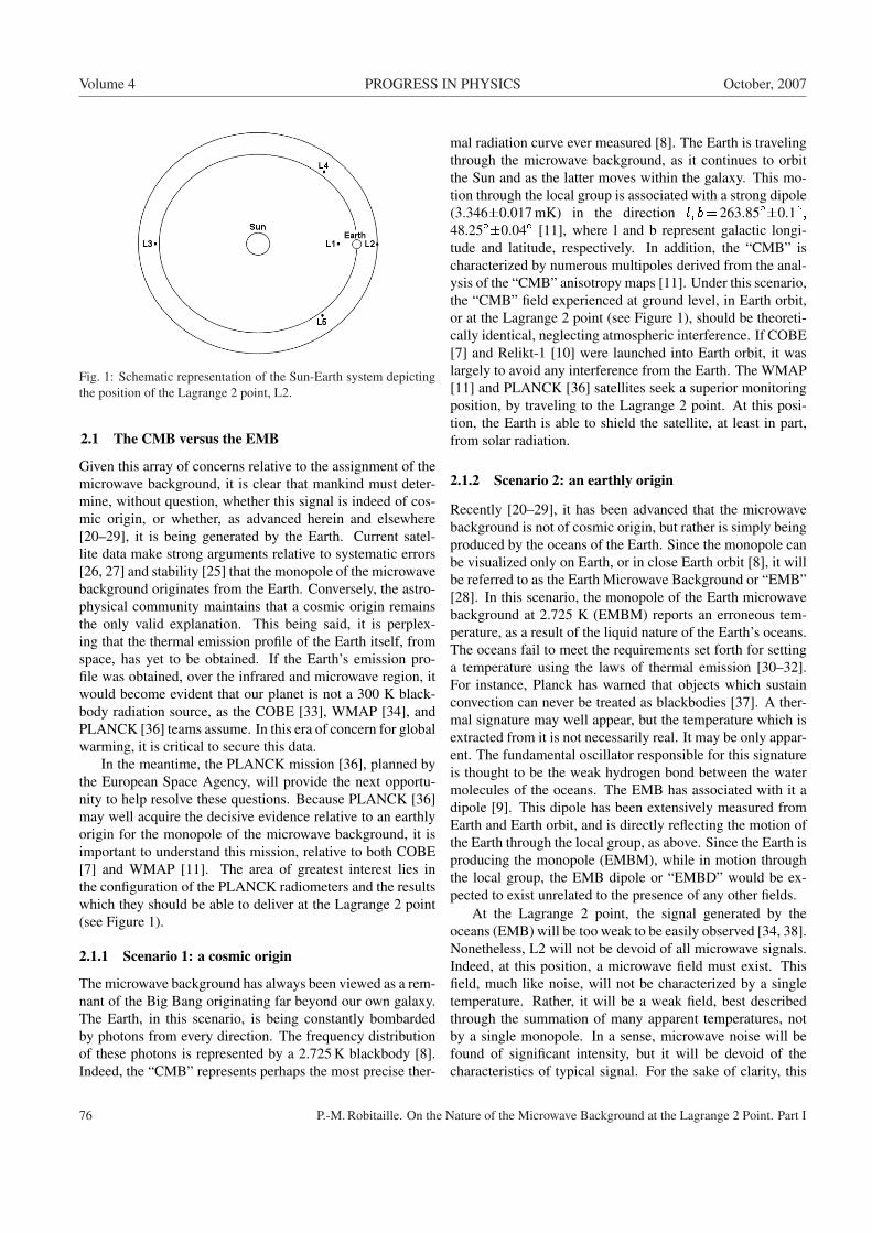
Volume 4 PROGRESS IN PHYSICS October, 2007
Fig. 1: Schematic representation of the Sun-Earth system depictingthe position of the Lagrange 2 point, L2.
2.1 The CMB versus the EMB
Given this array of concerns relative to the assignment of themicrowave background, it is clear that mankind must deter-mine, without question, whether this signal is indeed of cos-mic origin, or whether, as advanced herein and elsewhere[20–29], it is being generated by the Earth. Current satel-lite data make strong arguments relative to systematic errors[26, 27] and stability [25] that the monopole of the microwavebackground originates from the Earth. Conversely, the astro-physical community maintains that a cosmic origin remainsthe only valid explanation. This being said, it is perplex-ing that the thermal emission profile of the Earth itself, fromspace, has yet to be obtained. If the Earth’s emission pro-file was obtained, over the infrared and microwave region, itwould become evident that our planet is not a 300 K black-body radiation source, as the COBE [33], WMAP [34], andPLANCK [36] teams assume. In this era of concern for globalwarming, it is critical to secure this data.
In the meantime, the PLANCK mission [36], planned bythe European Space Agency, will provide the next opportu-nity to help resolve these questions. Because PLANCK [36]may well acquire the decisive evidence relative to an earthlyorigin for the monopole of the microwave background, it isimportant to understand this mission, relative to both COBE[7] and WMAP [11]. The area of greatest interest lies inthe configuration of the PLANCK radiometers and the resultswhich they should be able to deliver at the Lagrange 2 point(see Figure 1).
2.1.1 Scenario 1: a cosmic origin
The microwave background has always been viewed as a rem-nant of the Big Bang originating far beyond our own galaxy.The Earth, in this scenario, is being constantly bombardedby photons from every direction. The frequency distributionof these photons is represented by a 2.725 K blackbody [8].Indeed, the “CMB” represents perhaps the most precise ther-
mal radiation curve ever measured [8]. The Earth is travelingthrough the microwave background, as it continues to orbitthe Sun and as the latter moves within the galaxy. This mo-tion through the local group is associated with a strong dipole(3.346�0.017 mK) in the direction l; b= 263.85��0.1�;48.25��0.04� [11], where l and b represent galactic longi-tude and latitude, respectively. In addition, the “CMB” ischaracterized by numerous multipoles derived from the anal-ysis of the “CMB” anisotropy maps [11]. Under this scenario,the “CMB” field experienced at ground level, in Earth orbit,or at the Lagrange 2 point (see Figure 1), should be theoreti-cally identical, neglecting atmospheric interference. If COBE[7] and Relikt-1 [10] were launched into Earth orbit, it waslargely to avoid any interference from the Earth. The WMAP[11] and PLANCK [36] satellites seek a superior monitoringposition, by traveling to the Lagrange 2 point. At this posi-tion, the Earth is able to shield the satellite, at least in part,from solar radiation.
2.1.2 Scenario 2: an earthly origin
Recently [20–29], it has been advanced that the microwavebackground is not of cosmic origin, but rather is simply beingproduced by the oceans of the Earth. Since the monopole canbe visualized only on Earth, or in close Earth orbit [8], it willbe referred to as the Earth Microwave Background or “EMB”[28]. In this scenario, the monopole of the Earth microwavebackground at 2.725 K (EMBM) reports an erroneous tem-perature, as a result of the liquid nature of the Earth’s oceans.The oceans fail to meet the requirements set forth for settinga temperature using the laws of thermal emission [30–32].For instance, Planck has warned that objects which sustainconvection can never be treated as blackbodies [37]. A ther-mal signature may well appear, but the temperature which isextracted from it is not necessarily real. It may be only appar-ent. The fundamental oscillator responsible for this signatureis thought to be the weak hydrogen bond between the watermolecules of the oceans. The EMB has associated with it adipole [9]. This dipole has been extensively measured fromEarth and Earth orbit, and is directly reflecting the motion ofthe Earth through the local group, as above. Since the Earth isproducing the monopole (EMBM), while in motion throughthe local group, the EMB dipole or “EMBD” would be ex-pected to exist unrelated to the presence of any other fields.
At the Lagrange 2 point, the signal generated by theoceans (EMB) will be too weak to be easily observed [34, 38].Nonetheless, L2 will not be devoid of all microwave signals.Indeed, at this position, a microwave field must exist. Thisfield, much like noise, will not be characterized by a singletemperature. Rather, it will be a weak field, best describedthrough the summation of many apparent temperatures, notby a single monopole. In a sense, microwave noise will befound of significant intensity, but it will be devoid of thecharacteristics of typical signal. For the sake of clarity, this
76 P.-M. Robitaille. On the Nature of the Microwave Background at the Lagrange 2 Point. Part I
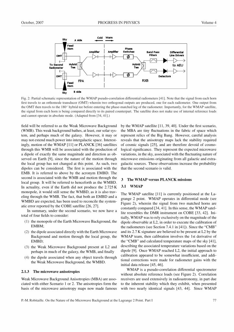
October, 2007 PROGRESS IN PHYSICS Volume 4
Fig. 2: Partial schematic representation of the WMAP pseudo-correlation differential radiometers [41]. Note that the signal from each hornfirst travels to an orthomode transducer (OMT) wherein two orthogonal outputs are produced, one for each radiometer. One output fromthe OMT then travels to the 180� hybrid tee before entering the phase-matched leg of the radiometer. Importantly, for the WMAP satellite,the signal from each horn is being compared directly to its paired counterpart. The satellite does not make use of internal reference loadsand cannot operate in absolute mode. (Adapted from [34, 41].)
field will be referred to as the Weak Microwave Background(WMB). This weak background bathes, at least, our solar sys-tem, and perhaps much of the galaxy. However, it may ormay not extend much power into intergalactic space. Interest-ingly, motion of the WMAP [11] or PLANCK [36] satellitesthrough this WMB will be associated with the production ofa dipole of exactly the same magnitude and direction as ob-served on Earth [9], since the nature of the motion throughthe local group has not changed at this point. As such, twodipoles can be considered. The first is associated with theEMB. It is referred to above by the acronym EMBD. Thesecond is associated with the WMB and motion through thelocal group. It will be referred to henceforth as the WMBD.In actuality, even if the Earth did not produce the 2.725 Kmonopole, it would still sense the WMBD, as it is also trav-eling through the WMB. The fact, that both an EMBD and aWMBD are expected, has been used to reconcile the system-atic error reported by the COBE satellite [26, 27].
In summary, under the second scenario, we now have atotal of four fields to consider:
(1) the monopole of the Earth Microwave Background, theEMBM;
(2) the dipole associated directly with the Earth MicrowaveBackground and motion through the local group, theEMBD;
(3) the Weak Microwave Background present at L2 andperhaps in much of the galaxy, the WMB, and finally
(4) the dipole associated when any object travels throughthe Weak Microwave Background, the WMBD.
2.1.3 The microwave anisotropies
Weak Microwave Background Anisotropies (MBA) are asso-ciated with either Scenario 1 or 2. The anisotropies form thebasis of the microwave anisotropy maps now made famous
by the WMAP satellite [11, 39, 40]. Under the first scenario,the MBA are tiny fluctuations in the fabric of space whichrepresent relics of the Big Bang. However, careful analysisreveals that the anisotropy maps lack the stability requiredof cosmic signals [25], and are therefore devoid of cosmo-logical significance. They represent the expected microwavevariations, in the sky, associated with the fluctuating nature ofmicrowave emissions originating from all galactic and extra-galactic sources. These observations increase the probabilitythat the second scenario is valid.
3 The WMAP versus PLANCK missions
3.1 WMAP
The WMAP satellite [11] is currently positioned at the La-grange 2 point. WMAP operates in differential mode (seeFigure 2), wherein the signal from two matched horns areconstantly compared [34, 41]. In this sense, the WMAP satel-lite resembles the DMR instrument on COBE [33, 42]. Ini-tially, WMAP was to rely exclusively on the magnitude of thedipole observable at L2, in order to execute the calibration ofthe radiometers (see Section 7.4.1 in [41]). Since the “CMB”and its 2.7 K signature are believed to be present at L2 by theWMAP team, then calibration involves the 1st derivative ofthe “CMB” and calculated temperature maps of the sky [41],describing the associated temperature variations based on thedipole [9]. Once WMAP reached L2, the initial approach tocalibration appeared to be somewhat insufficient, and addi-tional corrections were made for radiometer gains with theinitial data release [45, 46].
WMAP is a pseudo-correlation differential spectrometerwithout absolute reference loads (see Figure 2). Correlationreceivers are used extensively in radioastronomy, in part dueto the inherent stability which they exhibit, when presentedwith two nearly identical signals [43, 44]. Since WMAP
P.-M. Robitaille. On the Nature of the Microwave Background at the Lagrange 2 Point. Part I 77
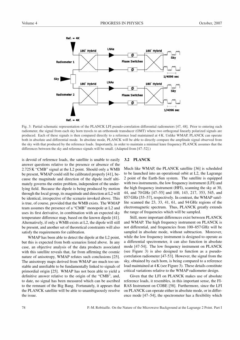
Volume 4 PROGRESS IN PHYSICS October, 2007
Fig. 3: Partial schematic representation of the PLANCK LFI pseudo-correlation differential radiometers [47, 48]. Prior to entering eachradiometer, the signal from each sky horn travels to an orthomode transducer (OMT) where two orthogonal linearly polarized signals areproduced. Each of these signals is then compared directly to a reference load maintained at 4 K. Unlike WMAP, PLANCK can operateboth in absolute and differential mode. In absolute mode, PLANCK will be able to directly compare the amplitude signal observed fromthe sky with that produced by the reference loads. Importantly, in order to maintain a minimal knee frequency PLANCK assumes that thedifferences between the sky and reference signals will be small. (Adapted from [47–52].)
is devoid of reference loads, the satellite is unable to easilyanswer questions relative to the presence or absence of the2.725 K “CMB” signal at the L2 point. Should only a WMBbe present, WMAP could still be calibrated properly [41], be-cause the magnitude and direction of the dipole itself ulti-mately governs the entire problem, independent of the under-lying field. Because the dipole is being produced by motionthrough the local group, its magnitude and direction at L2 willbe identical, irrespective of the scenario invoked above. Thisis true, of course, provided that the WMB exists. The WMAPteam assumes the presence of a “CMB” monopole at L2 anduses its first derivative, in combination with an expected skytemperature difference map, based on the known dipole [41].Alternatively, if only a WMB exists at L2, the dipole will stillbe present, and another set of theoretical constraints will alsosatisfy the requirements for calibration.
WMAP has been able to detect the dipole at the L2 point,but this is expected from both scenarios listed above. In anycase, an objective analysis of the data products associatedwith this satellite reveals that, far from affirming the cosmicnature of anisotropy, WMAP refutes such conclusions [25].The anisotropy maps derived from WMAP are much too un-stable and unreliable to be fundamentally linked to signals ofprimordial origin [25]. WMAP has not been able to yield adefinitive answer relative to the origin of the “CMB”, and,to date, no signal has been measured which can be ascribedto the remnant of the Big Bang. Fortunately, it appears thatthe PLANCK satellite will be able to unambiguously resolvethe issue.
3.2 PLANCK
Much like WMAP, the PLANCK satellite [36] is scheduledto be launched into an operational orbit at L2, the Lagrange2 point of the Earth-Sun system. The satellite is equippedwith two instruments, the low frequency instrument (LFI) andthe high frequency instrument (HFI), scanning the sky at 30,44, and 70 GHz [47–55] and 100, 143, 217, 353, 545, and857 GHz [55–57], respectively. In contrast, the WMAP satel-lite scanned the 23, 33, 41, 61, and 94 GHz regions of theelectromagnetic spectrum. Thus, PLANCK greatly extendsthe range of frequencies which will be sampled.
Still, more important differences exist between PLANCKand WMAP. The high frequency instrument on PLANCK isnot differential, and frequencies from 100–857 GHz will besampled in absolute mode, without subtraction. Moreover,while the low frequency instrument is designed to operate asa differential spectrometer, it can also function in absolutemode [47-54]. The low frequency instrument on PLANCK(see Figure 3) is also designed to function as a pseudo-correlation radiometer [47-53]. However, the signal from thesky, obtained by each horn, is being compared to a referenceload maintained at 4 K (see Figure 3). These details constitutecritical variations relative to the WMAP radiometer design.
Given that the LFI on PLANCK makes use of absolutereference loads, it resembles, in this important sense, the FI-RAS Instrument on COBE [58]. Furthermore, since the LFIon PLANCK can operate either in absolute mode, or in differ-ence mode [47–54], the spectrometer has a flexibility which
78 P.-M. Robitaille. On the Nature of the Microwave Background at the Lagrange 2 Point. Part I
October, 2007 PROGRESS IN PHYSICS Volume 4
appears to combine the best features possible for such an in-strument. In absolute mode, the LFI on PLANCK will beable to quantify completely the signal originating from thesky relative to that produced by its 4 K references. Nonethe-less, the LFI was designed to operate primarily in differentialmode. This has implications for the quality of its data prod-ucts based on whether or not the 2.725 K monopole signal ispresent at L2.
3.2.1 The PLANCK LFI
The PLANCK LFI is designed as a pseudo-correlation [52]receiver (see Figure 3). For this receiver, gain instabilitiesin the High Electron Mobility Transistor (HEMT) amplifier,within the receiver front end, result in 1=f noise. The 1=fnoise, if not properly accounted for, can produce significantstripes in the final maps [47, 48]. These stripes are also de-pendent on scanning strategy. The behavior of the 1=f noisehas been carefully analyzed for the PLANCK LFI [47, 48].Since the LFI is designed to operate primarily in differen-tial mode, it is important to minimize the difference betweenthe reference load temperature, Tref , and the sky tempera-ture, Tsky .
Currently, the PLANCK team is making the assumptionthat Tsky = 2.725 K, as previously reported by the COBEgroup [7]. As such, they have chosen to use Tref = 4 K. Anyoffset between Tsky and Tref “can be balanced before differ-encing either by a variable back-end gain stage with a feed-back scheme to maintain the output power as close as pos-sible to zero, or by multiplying in software one of the twosignals by a so-called gain modulation factor” [47].
If the differences between the sky temperature and the ref-erence temperatures are large, then the idea of using back-endgain stage feedback, to balance the two channels, should in-troduce substantial noise directly into the system. The situa-tion using software and a gain modulation factor would alsointroduce unexpected complications.
The gain modulation factor, r, is given by the following:r = (Tsky +Tn)=(Tref +Tn) where Tn corresponds to theradiometer noise temperature. The noise temperature of theradiometer, Tn, is a fundamental property of any receiver andis determined by the overall design and quality of the instru-ment. Tn is critical in establishing the sensitivity of the spec-trometer. For instance, the radiometer sensitivity, �Trms,over a given integration time, is directly dependent on bothTsky and Tn, as follows: �Trms = 2(Tsky +Tn)=
p�, where
� is the bandwidth of the radiometer (typically taken as 20%).Note that if Tn is large, then it will be easy to achieve gainmodulation factors near 1. However, the radiometer sensi-tivity would be severely compromised. Low Tn values arecentral to the performance of any receiver. Under this con-straint, the gain modulation factor will be strongly affectedby any differences between the Tsky and Tref .
PLANCK has the ability to calculate the gain modulation
factor, r, directly from radiometer data acquired with the spec-trometer operating in absolute mode [47]. Alternatively, r canbe calculated from software, using up to three approaches in-cluding, for instance, minimizing the final differenced dataknee frequency, fk. The knee frequency is the frequency atwhich the value of 1=f noise and white noise contributionsare equal.
In general, it is also true that for the PLANCK LFI “thewhite noise sensitivity and the knee-frequency depend on theactual temperature in the sky” [47]. Because excessive 1=fnoise can degrade the final images and data products [47,48], it is important to minimize its contribution. This canbe achieved “if the post detection knee frequency fk (i.e. thefrequency at which the 1=f noise contribution and the idealwhite noise contribution are equal) is significantly lower thanthe spacecraft rotation frequency (fspin� 0.017 Hz)” [48].If the fk is greater than, or approximately equal to fspin, adegradation in the final sensitivity of the satellite will occur[47]. As this inherently depends on the real sky temperature,there are some concerns relative to the performance of thePLANCK LFI instruments.
When the knee frequencies are too high, stripes will occurin the images generated by the satellite. It is true that algo-rithms do exist to help remove these artifacts, provided thatthey are not too strong [47]. Nonetheless, when the sky tem-perature and the reference temperatures are not balanced, theknee frequency will rise substantially. This could diminishthe quality of the data products from this satellite.
The importance of maintaining a low knee frequency forthe PLANCK LFI instruments cannot be overstated. “If theknee frequency is sufficiently low (i.e. fk 6 0.1 Hz), with theapplication of such algorithms it is possible to maintain boththe increase in rms noise within few % of the white noise, andthe power increase at low multipole values (i.e. l6 200) ata very low level (two orders of magnitude less than the CMBpower). If, on the other hand, the knee frequency is high (i.e.� 0.1 Hz) then even after destriping the degradation of thefinal sensitivity is of several tens of % and the excess powerat low multipole values is significant (up to the same orderof the CMB power for fk� 10 Hz . . . ) Therefore, carefulattention to instrument design, analysis, and testing is essen-tial to achieve a low 1=f noise knee frequency” [48]. ThePLANCK team has emphasized this further, as follows: “It isthen of great importance to decrease as much as possible theimpact of 1=f noise before destriping and fk = 0.01 Hz is animportant goal for instrument studies and prototypes.”
The manner in which the knee frequency is affected byboth the gain modulation factor, r, and the absolute sky tem-perature [48], has been described algebraically:
fk (Tn) = ��A (1� r)Tn2 (Tsky + Tn)
�2
: (1)
In this equation, � corresponds to the bandwidth of thereceiver, typically taken at 20%, Tn is the radiometer noise
P.-M. Robitaille. On the Nature of the Microwave Background at the Lagrange 2 Point. Part I 79

Volume 4 PROGRESS IN PHYSICS October, 2007
temperature, and A is a normalization factor for noise fluc-tuations [48]. Note that if the sky temperature, Tsky , is onlysome fraction of a Kelvin degree, this equation is moving to-wards:
fk (Tn) = ��A (1� r)
2
�2
: (2)
Under test conditions, the PLANCK team estimated gainmodulation factors ranging from 0.936 to 0.971 for the 30, 44,and 70 GHz radiometers [47]. In flight, Tn values of 7.5, 12,and 21.5 K are expected for the 30, 44, and 70 GHz radiome-ters [50]. This results in r values ranging from�0.89–0.95, ifTsky is taken as 2.725 K and Tref = 4 K. Anticipated fk val-ues would therefore range from �0.0032 Hz to �0.0043 Hz,well below the 16 mHz requirement. This situation will notoccur under Scenario 2, wherein Tsky at L2 is not 2.725 K,but rather only some fraction of a Kelvin degree.
As Tsky will have a much lower value than foreseen, thegain modulation factor, r, will be moving away from unity.It is also clear from Eqs. 1 and 2 that the knee frequency forthe LFI radiometers would rise to values substantially abovethose currently sought by the PLANCK team.
In the extreme case, it is simple to consider the conse-quence of Tsky! 0. In this instance, gain modulation factorswould drop precipitously from �0.89 to �0.65 at 30 GHz,and from �0.95 to �0.84 at 70 GHz. This would translateinto substantially elevated fk values of �50 mHz. Even anapparent Tsky value of 300 mK would result in r and fk val-ues in this range. Other than the direct measurement of thesky temperature by the PLANCK LFI in absolute mode, thedrop in r values and the tremendous rise in fk will constituteanother indication that the 2.725 K signal does not exist at theL2 point.
Consequently, it is difficult to envision that the PLANCKteam will be able to attain the desired image quality if Tskyis not at 2.725 K. The spectrometer is not designed to achievemaximal sensitivity in absolute mode, while in differencemode, both its r values and its fk will be compromised. De-striping algorithms will have to be invoked in a much morecentral manner than anticipated.
Note that the situation with PLANCK is substantially dif-ferent from WMAP. With WMAP (see Figure 2), the radio-meters do not make use of an absolute reference load, butrather, the two sky horns are constantly and directly beingdifferenced. Thus, the knee frequency for WMAP would beas predicted prior to launch. The WMAP horns are nearlyperfectly balanced by the sky itself. Therefore, their perfor-mance would not be affected by the real nature of the signalat L2. This is not the case for the PLANCK satellite.
4 Conclusion
The WMAP satellite was designed as a differential spectrom-eter without absolute calibration. As a result, it is unable
to ascertain the absolute magnitude of the microwave sig-nals at the L2 point. The satellite has produced anisotropymaps [39, 40]. Yet, these maps lack the stability required ofcosmological signals. Indeed, WMAP appears devoid of anyfindings relative to cosmology, as previously stated [25]. Theonly signal of note, and one which was not anticipated [21],is that associated with the dipole [9, 26, 27]. The dipole isimportant, since it can be used to quantify the motion of ob-jects through the local group. Under the second scenario, thisdipole signal implies that there is a Weak Microwave Back-ground (WMB) at the L2 point.
In sharp contrast with WMAP, PLANCK has the advan-tage of being able to operate in absolute mode. In this con-figuration, it can directly determine whether or not there isa 2.725 K monopole signal at L2. If the signal is present,as expected by the PLANCK team, and as predicted in thefirst scenario, then the satellite should be able to acquire sim-ply phenomenal maps of the sky. However, this will not oc-cur. In the absence of a monopole, the PLANCK radiome-ters will be compromised when operating in difference mode,as their knee frequencies rise. This shall result in the pres-ence of more pronounced image artifacts in the data prod-ucts, which may not be easily removed through processing,potentially impacting the harvest from PLANCK. Nonethe-less, PLANCK should be able to fully characterize the WMBpredicted under the second scenario.
At the same time, since the 2.725 K monopole signaturedoes not exist at the L2 point, PLANCK is poised to alterthe course of human science. The satellite will help estab-lish that there is no universality [30, 31]. The need to linkPlanck’s equation to the physical world will become evident[30, 31]. It will be realized that the Penzias and Wilson signaldid come from the Earth, and that liquids can indeed producethermal spectra reporting incorrect temperatures. It is likelythat a renewed interest will take place in condensed matterphysics, particularly related to a more profound understand-ing of thermal emission, in general, and to the study of ther-mal processes in liquids, in particular. The consequences forastrophysics will be far reaching, impacting our understand-ing of stellar structure [59, 60], stellar evolution and cosmol-ogy. PLANCK, now, must simply lead the way.
Acknowledgements
The author thanks Dmitri Rabounski for valuable discussions.Luc Robitaille is recognized for figure preparation.
Dedication
This work is dedicated to my brother, Patrice, for his love andencouragement.
Submitted on August 06, 2007Accepted on August 15, 2007
Published online on September 08, 2007Revised on September 29, 2007
80 P.-M. Robitaille. On the Nature of the Microwave Background at the Lagrange 2 Point. Part I
October, 2007 PROGRESS IN PHYSICS Volume 4
References
1. Penzias A.A. and Wilson R.W. A measurement of excess an-tenna temperature at 4080 Mc/s. Astrophys. J., 1965, v. 1, 419–421.
2. Dicke R.H., Peebles P.J.E., Roll P.G., and Wilkinson D.T. Cos-mic black-body radiation. Astrophys. J., 1965, v. 1, 414–419.
3. Partridge R.B. 3K: The Cosmic Microwave Background Radi-ation. Cambridge University Press, Cambridge, 1995.
4. Lineweaver C.H., Bartlett J.G., Blanchard A., Signore M. andSilk J. The Cosmic Microwave Background. Kluwer AcademicPublishers. Boston, 1997.
5. de Bernardis P., Ade P.A.R., Bock J.J., Bond J.R., BorrillJ.,Boscaleri A., Coble K., Crill B.P., De Gasperis G., FareseP.C., Ferreira P.G., Ganga K., Giacometti M., Hivon E., HristovV.V., Iacoangeli A., Jaffe A.H., Lange A.E., Martinis L., Masi1S., Mason P.V., Mauskopf P.D., Melchiorri A., Miglio L., Mon-troy T., Netterfield C.B., Pascale E., Piacentini F., Pogosyan D.,Prunet S., Rao S., Romeo G., Ruhl J.E., Scaramuzzi F., Sforna1D., and Vittorio N. A flat universe from high-resolution mapsof the Cosmic Microwave Background. Nature, 2000, v. 404,955–959.
6. Spergel D.N., Verde L., Peiris H.V., Komatsu E., Nolta M.R.,Bennett C.L., Halpern M., Hinshaw G., Jarosik N., Kogut A.,Limon M., Meyer S.S., Page L., Tucker G.S., Weiland J.L.,Wollack E., and Wright E.L. First year Wilkinson MicrowaveAnisotropy Probe (WMAP) observations: Determination ofcosmological parameters. Astrophys. J. Suppl., 2003, v. 148,175–194.
7. COBE website, http://lambda.gsfc.nasa.gov/product/cobe/
8. Fixen D.J., Cheng E.S., Gales J.M., Mather J.C., Shaffer R.A.,and Wright E.L. The Cosmic Microwave Background spectrumfrom the full COBE FIRAS data set. Astrophys. J., 1996, v. 473,576–587.
9. Lineweaver C.H. The CMB Dipole: The most recent measure-ment and some history. In Microwave Background Anistropies.Proceedings of the XVIth Moriond Astrophysics Meeting, LesArcs, Savoie, France, March 16th-23rd, 1996, F. R. Bouchet,R. Gispert, B. Guilderdoni, and J.T.T. Van, eds., Gif-sur-Yvette:Editions Frontieres, 1997; (see also arXiv:astro-ph/9609034).
10. Klypin A.A., Strukov I.A., and Skulachev D.P. The Relikt mis-sions: results and prospects for detection of the microwavebackground anisotropy. Mon. Not. R. Astr. Soc., 1992, v. 258,71–81.
11. WMAP website, http://map.gsfc.nasa.gov/
12. Spergel D.N., Bean R., Dore O., Nolta M.R., Bennett C.L.,Dunkley J., Hinshaw G., Jarosik N., Komatsu E., Page L., PeirisH.V., Verde L., Halpern M., Hill R.S., Kogut A., Limon M.,Meyer S.S., Odegard N., Tucker G.S., Weiland J.L., WollackE., and Wright E.L. Wilkinson Microwave Anisotropy Probe(WMAP) three year results: implications for cosmology. Astro-physical J. Suppl. Series, 2007, v. 170, 377–408.
13. Burles S., Nollett K.M., and Turner M.S. Big Bang nucleosyn-thesis predictions for precision cosmology. Astrophys. J., 2001,v. 552, L1–L5.
14. Guth A.H. Inflation and the new era of high precision cosmol-ogy. MIT Physics Annual, 2002, 28–39.
15. Smoot G.F. Our age of precision cosmology. Proceedings of the2002 International Symposium on Cosmology and Particle As-trophysics (CosPA 02), X.G. He and K.W. Ng, Editors, WorldScientific Publications, 2003, London, U.K., 314–326.
16. Seife C. Breakthrough of the year: illuminating the dark uni-verse. Science, 2003, v. 302, 2038–2039.
17. NASA, new satellite data on Universe’s first trillionth sec-ond. WMAP Press Release. http://map.gsfc.nasa.gov/m or/PressRelease 03 06.html.
18. Goodman B. Big days for the Big Bang. Princeton AlumniWeekly, May, 2003.
19. Panek R. Out There. New York Times Magazine, March 11,2007, 55–59.
20. Robitaille P.-M.L. Nuclear magnetic resonance and the age ofthe Universe. American Physical Society Centennial Meeting,Atlanta, Georgia, BC19.14, March 19–26, 1999.
21. Robitaille P-M.L. The MAP satellite: a powerful lesson in ther-mal physics. Spring Meeting of the American Physical SocietyNorthwest Section, F4.004, May 26, 2001.
22. Robitaille P.-M.L. The collapse of the Big Bang and the gaseoussun. New York Times, March 17th, 2002 (accessed online fromhttp://thermalphysics.org/pdf/times.pdf).
23. Robitaille P-M.L. WMAP: a radiological analysis. SpringMeeting of the American Physical Society Ohio Section,S1.00003, March 31 — April 1, 2006.
24. Robitaille P-M.L. WMAP: a radiological analysis II. SpringMeeting of the American Physical Society Northwest Section,G1.0005, May 19–20, 2006.
25. Robitaille P.-M.L. WMAP: a radiological analysis. Progr. inPhys., 2007, v. 1, 3–18.
26. Robitaille P.-M.L. On the origins of the CMB: insight from theCOBE, WMAP, and Relikt-1 Satellites. Progr. in Phys., 2007,v. 1, 19–23.
27. Rabounski D. The relativistic effect of the deviation betweenthe CMB temperatures obtained by the COBE satellite. Progr.in Phys., 2007, v. 1, 24–26.
28. Robitaille P.-M.L. On the Earth Microwave Background: ab-sorption and scattering by the atmosphere. Progr. in Phys.,2007, v. 3, 3–4.
29. Robitaille P.-M.L., Rabounski D. COBE and the absolute as-signment of the CMB to the Earth. American Physical SocietyMarch Meeting, L20.00007, March 5–9, 2007.
30. Robitaille P.-M.L. On the validity of Kirchhoff’s law of thermalemission. IEEE Trans. Plasma Science, 2003, v. 31(6), 1263–1267.
31. Robitaille P.-M.L. An analysis of universality in blackbody ra-diation. Progr. Phys., 2006, v. 2, 22–23.
32. Kirchhoff G. Ueber das Verhaltnis zwischen dem Emissionsver-mogen und dem asbsorptionsvermogen der Korper fur Waemeund Litcht. Annalen der Physik, 1860, v. 109, 275–301.
33. Bennett C., Kogut A., Hinshaw G., Banday A., Wright E.,Gorski K., Wilkinson D., Weiss R., Smoot G., Meyer S., Mather
P.-M. Robitaille. On the Nature of the Microwave Background at the Lagrange 2 Point. Part I 81
Volume 4 PROGRESS IN PHYSICS October, 2007
J., Lubin P., Loewenstein K., Lineweaver C., Keegstra P., KaitaE., Jackson P., and Cheng E. Cosmic temperature fluctuationsfrom two years of COBE differential microwave radiometersobservations. Astrophys. J., 1994, v. 436, 4230–442.
34. Page L., Jackson C., Barnes C., Bennett C., Halpern M., Hin-shaw G., Jarosik N., Kogut A., Limon M., Meyer S.S., SpergelD.N., Tucker G.S., Wilkinson D.T., Wollack E., and WrightE.L. The optical design and characterization of the microwaveanisotropy probe. Astrophys. J., 2003, v. 585, 566–586.
35. Ulaby F.T., Moore R.K., Funk A.K. Microwave remote sensingactive and passive — Volume 2: Radar remote sensing and sur-face scattering and emission theory. London, Addison-WesleyPublishing Company, 1982, p. 880–884.
36. PLANCK website, see in http://www.rssd.esa.int
37. Planck M. The Theory of Heat Radiation. Philadelphia, PA., P.Blackinson’s Son, 1914.
38. Borissova L., Rabounski D. On the nature of the MicrowaveBackground at the Lagrange 2 point. Part II. Prog. in Phys.,2007, v. 4., 84–95.
39. Bennett C.L., Halpern M., Hinshaw G., Jarosik N., Kogut A.,Limon M., Meyer S.S., Page L., Spergel D.N., Tucker G.S.,Wollack E., Wright E.L., Barnes C., Greason M.R., Hill R.S.,Komatsu E., Nolta M.R., Odegard N., Peirs H.V., Verde L.,Weiland J.L. First year Wilkinson Microwave Anisotropy Probe(WMAP) observations: preliminary maps and basic results. As-trophys. J. Suppl. Series, 2003, v. 148, 1–27.
40. Hinshaw G., Nolta M.R., Bennett C.L., Bean R., Dore O., Grea-son M.R., Halpern M., Hill R.S., Jarosik N., Kogut A., KomatsuE., Limon M., Odegard N., Meyer S.S., Page L., Peiris H.V.,Spergel D.N., Tucker G.S., Verde L., Weiland J.L., WollackE., Wright E.L. Three-year Wilkinson Microwave AnisotropyProbe (WMAP) observations: temperature analysis. Astrophys.J. Suppl. Series, 2007, v. 170, 288–334.
41. Jarosik N., Bennett C.L., Halpern M., Hinshaw G., Kogut A.,Limon M., Meyer S.S., Page L., Pospieszalski M., SpergelD.N., Tucker G.S., Wilkinson D.T., Wollack E., Wright E.L.,and Zhang Z. Design, implementation and testing of the MAPradiometers. Astrophys. J. Suppl., 2003, v. 145, 413–436.
42. Kogut A., Banday A.J., Bennett C.L., Gorski K.M., HinshawG., Jackson P.D., Keegstra P., Lineweaver C., Smoot G.F.,Tenorio L., and Wright E.L. Calibration and systematic erroranalysis for the COBE DMR 4 year sky maps. Astrophys. J.,1996, v. 470, 653–673.
43. Egan W.F. Practical RF system design. Wiley-Interscience,Hoboken, New Jersey, 2003.
44. Rohlfs K. and Wilson T.L. Tools of radioastronomy. Springer-Verlag, Berlin, 1996.
45. Jarosik N., Barnes C., Bennett C.L., Halpern M., HinshawG., Kogut A., Limon M., Meyer S.S., Page L., Spergel D.N.,Tucker G.S., Weiland J.L., Wollack E., Wright E.L. First-yearWilkinson Microwave Anisotropy Probe (WMAP) observa-tions: on-orbit radiometer characterization. Astrophys. J. Suppl.Series, 2003, v. 148, 29–36.
46. Jarosik N., Barnes C., Greason M.R., Hill R.S., Nolta M.R.,Odegard N., Weiland J.L., Bean R., Bennett C.L., Dore O.,
Halpern M., Hinshaw G., Kogut A., Komatsu E., Limon M.,Meyer S.S., Page L., Spergel D.N., Tucker G.S., WollackE., Wright E.L. Three-year Wilkinson Microwave AnisotropyProbe (WMAP) observations: beam profiles, data processing,radiometer characterization and systematic error limits. Astro-phys. J. Suppl. Series, 2007, v. 170, 263–287.
47. Maino D., Burigana C., Maltoni M., Wandelt D.B., GorskiK.M., Malaspina M., Bersanelli M., Mandolesi N., BandayA.J., Hivon E.. The Planck-LFI instrument: analysis of the 1=fnoise and implications for the scanning strategy. Astrophys. J.Suppl. Series, 1999, v. 140, 383–391.
48. Sieffert M., Mennella A., Burigana C., Mandolesi N. BersanelliM., Meinhold P., and Lubin P. 1=f noise and other systematiceffects in the PLANCK-LFI radiometers. Astron. Astrophys.,2002, v. 391, 1185–1197.
49. Mennella A., Bersanelli M., Butler R.C., Maino D., MandolesiN., Morgante G., Valenziano L., Villa F., Gaier T., SeiffertM., Levin S., Lawrence C., Meinhold P., Lubin P., Tuovi-nen J., Varis J., Karttaavi T., Hughes N., Jukkala P., SjomanP., Kangaslahti P., Roddis N., Kettle D., Winder F., Black-hurst E., Davis R., Wilkinson A., Castelli C., Aja B., ArtalE., de la Fuente L., Mediavilla A., Pascual J.P., Gallegos J.,Martinez-Gonzalez E., de Paco P., and Pradell L. Advancedpseudo-correlation radiometers for the PLANCK-LFI instru-ment. arXiv: astro-ph/0307116.
50. Mennella A., Bersanelli M., Cappellini B., Maino D., Plata-nia P., Garavaglia S., Butler R.C., Mandolesi N., Pasian F.,D’Arcangelo O., Simonetto A., and Sozzi C. The low fre-quency instrument in the ESA PLANCK mission. arXiv: astro-ph/0310058.
51. Bersanelli M., Aja B., Artal E., Balasini M., Baldan G.,Battaglia P., Bernardino T., Bhandari P., Blackhurst E., Bos-chini L., Bowman R., Burigana C., Butler R.C., Cappellini B.,Cavaliere F., Colombo F., Cuttaia F., Davis R., Dupac X., Edge-ley J., D’Arcangelo O., De La Fuente L., De Rosa A., Fer-rari F., Figini L., Fogliani S., Franceschet C., Franceschi E.,Jukkala P., Gaier T., Galtress A., Garavaglia S., Guzzi P., Her-reros J.M., Hoyland R., Huges N., Kettle D., Kilpela V.H., Laa-ninen M., Lapolla P.M., Lawrence C.R., Lawson D., LeonardiF., Leutenegger P., Levin S., Lilje P.B., Lubin P.M., Maino D.,Malaspina M., Mandolesi M., Mari G., Maris M., Martinez-Gonzalez E., Mediavilla A., Meinhold P., Mennella A., Mic-colis M., Morgante G., NashA., Nesti R., Pagan L., Paine C.,Pascual J.P., Pasian F., Pecora M., Pezzati S., Pospieszalski M.,Platania P., Prina M., Rebolo R., Roddis N., Sabatini N., San-dri M., Salmon M.J., Seiffert M., Silvestri R., Simonetto A.,Smoot G.F., Sozzi C., Stringhetti L., Terenzi L., Tomasi M.,Tuovinen J., Valenziano L., Varis J., Villa F.,Wade L., Wilkin-son A., Winder F., and Zacchei A. PLANCK-LFI: Instrumentdesign and ground calibration strategy. Proc. Eur. MicrowaveAssoc., 2005, v. 1, 189–195.
52. Mennella A., Bersanelli M., Seiffert M., Kettle D., Roddis N.,Wilkinson A., and Meinhold P. Offset balancing in pseudo-correlation radiometers for CMB measurements. Astro. Astro-phys., 2003, v. 410, 1089–1100.
53. Terenzi L., Villa F., Mennella A., Bersanelli M., Butler R.C.,Cuttaia F., D’Arcangelo O., Franceschi E., Galeotta S., Maino
82 P.-M. Robitaille. On the Nature of the Microwave Background at the Lagrange 2 Point. Part I
October, 2007 PROGRESS IN PHYSICS Volume 4
D., Malaspina M., Mandolesi N., Morgante G., Sandri M.,Stringhetti L., Tomasi M., Valenziano L., Burigana C., FinelliF., Galaverni M., Gruppuso A., Paci F., Popa L., Procopio P.,and Zuccarelli J. The PLANCK LFI RCA flight model test cam-paign. New Astronomy Rev., 2007, v. 51, 305–309.
54. Valenziano L., Sandri M., Morgante G., Burigana C., BersanelliM., Butler R.C., Cuttaia F., Finelli F., Franceschi E., GalaverniM., Gruppuso A., Malaspina M., Mandolesi N., Mennella A.,Paci F., Popa L., Procopio P., Stringhetti L., Terenzi L., TomasiM., Villa F., and Zuccarelli J. The low frequency instrumenton-board the Planck satellite: Characteristics and performance.New Astronomy Rev., 2007, v. 51, 287–297.
55. Lamarre J.M, Puget J.L., Bouchet F., Ade P.A.R., Benoit A.,Bernard J.P., Bock J., De Bernardis P., Charra J., Couchot F.,Delabrouille J., Efstathiou G., Giard M., Guyot G., Lange A.,Maffei B., Murphy A, Pajot F., Piat M., Ristorcelli I., Santos D.,Sudiwala R., Sygnet J.F., Torre J.P., Yurchenko V., and Yvon D.The PLANCK High Frequency Instrument, a third generationCMB experiment, and a full sky submillimeter survey. New As-tronomy Rev., 2003, v. 47, 1017–1024.
56. Piat M., Torre J.P., Breelle E., Coulais A., Woodcraft A.,Holmes W., and Sudiwala R. Modeling of PLANCK-high fre-quency instrument bolometers using non-linear effects in thethermometers. Nuclear Instr. Meth. Phys. Res. A, 2006, v. 559,588–590.
57. Brossard J., Yurchenko V., Gleeson E, Longval Y., Maffei B.,Murphy A., Ristorcelli I., and Lamarre J.M. PLANCK-HFI:Performances of an optical concept for the Cosmic MicrowaveBackground anisotropies measurement. Proc. 5th Intern. Conf.on Space Optics (ICSO 2004), 30 March — 2 April 2004,Toulouse, France (ESA SP-554, June 2004).
58. Fixsen D.J., Cheng E.S., Cottingham D.A., Eplee R.E.,Hewagama T., Isaacman R.B., Jensen K.A., Mather J.C., MassaD.L., Meyer S.S., Noerdlinger P.D., Read S.M., Rosen L.P.,Shafer R.A., Trenholme A.R., Weiss R., Bennett C.L., BoggessN.W., Wilkinson D.T., and Wright E.L. Calibration of theCOBE Firas Instrument. Astrophys. J., 1994, v. 420, 457–473.
59. Robitaille P.M. The solar photosphere: evidence for condensedmatter. Prog. in Phys., 2006, v. 2, 17–21.
60. Robitaille P.-M. A high temperature liquid plasma model of theSun. Prog. in Phys., 2007, v. 1, 70–81.
P.-M. Robitaille. On the Nature of the Microwave Background at the Lagrange 2 Point. Part I 83

Volume 4 PROGRESS IN PHYSICS October, 2007
On the Nature of the Microwave Background at the Lagrange 2 Point. Part II
Larissa Borissova and Dmitri RabounskiE-mail: [email protected]; [email protected]
In this work the mathematical methods of General Relativity are used to answer thefollowing questions: if a microwave background originates from the Earth, what wouldbe its density and associated dipole measured at the altitude of a U2 aeroplane (25 km),the COBE satellite (900 km), and the 2nd Lagrange point (1.5 million km, the posi-tion of the WMAP and PLANCK satellites)? The first problem is solved via Einstein’sequations for the electromagnetic field of the Earth. The second problem is solved usingthe geodesic equations for light-like particles (photons) which are mediators for electro-magnetic radiation. We have determined that a microwave background that originates atthe Earth (the Earth microwave background) decreases with altitude so that the densityof the energy of such a background at the altitude of the COBE orbit (900 km) is 0.68times less than that at the altitude of a U2 aeroplane. The density of the energy of thebackground at the L2 point is only �10�7 of the value detected by a U2 aeroplane or atthe COBE orbit. The dipole anisotropy of the Earth microwave background, due to therapid motion of the Earth relative to the source of another field which isn’t connectedto the Earth but is located in depths of the cosmos, doesn’t depend on altitute from thesurface of the Earth. Such a dipole will be the same irrespective of the position at whichmeasurements are taken.
1 Problem statement: the space of the Earth and theEarth microwave background
Here we solve two theoretical problems related to the mea-surement of the microwave background:
(1) What is the density of the Earth microwave backgroundwhich one will observe at the COBE orbit and at the L2point?
(2) What is the anisotropy of the Earth microwave back-ground, due to a drift of the whole space of the Earth,which one will observe in the COBE orbit and at theL2 point?
In a sense, the anisotropy we are treating is the sum of thedipole and all other multipoles.
According to General Relativity, the result of an observa-tion depends on the velocity of the observer relative to the ob-ject he observes, and also on the properties of the local space(such as the space rotation, gravitation, deformation, curva-ture, etc.) where the observation is made. Therefore, we arelooking for a theoretical solution of the aforementioned prob-lems using the mathematical methods, which are specific toGeneral Relativity.
We solve the first problem using Einstein’s equations, ma-nifest in the energy and momentum of a field of distributedmatter (an electromagnetic field, for instance), depending onthe distance from the field’s source, and also on the propertiesof the space e.g. the space rotation, gravitation, etc.
We solve the second problem using the geodesic equa-tions for light-like particles (photons, which are mediators formicrowave radiation, and for any electromagnetic radiation ingeneral). The geodesic equations give a possibility of finding
a preferred direction (anisotropy) in such a field due to thepresence of a linear drift of the whole reference space of theobserver relative to the source of another field, which isn’tconnected to the observer’s space, but moves with respect toit [1, 2]. In the present case, such a linear drift is due to themotion of the observer, in common with the microwave back-ground’s source, the Earth, relative to the source of anotherfield such as the common field of a group of galaxies or thatof the Universe as a whole (a weak microwave background).Then we compare our theoretical result from General Relativ-ity to the experimental data for the microwave background,obtained in space near the Earth by the COBE satellite, lo-cated in a 900 km orbit, and also by the WMAP satellite, lo-cated at the L2 point, as far as 1.5 million km from the Earth.
In order to obtain a theoretical result expressed in quan-tities measurable in practice, we use the mathematical appa-ratus of chronometric invariants — the projections of four-dimensional quantities on the time line and spatial section ofa real observer, which are the physical observable quatities inGeneral Relativity [3, 4].
First, we introduce a space where all the mesurements aretaken. Both locations, of the COBE satellite and the L2 point,are connected, by gravitation, to the gravitational field of theEarth, so both observers are connected to the space of theEarth, whose properties (e.g. rotation, gravitation, deforma-tion, etc.) affect the observations. We therefore consider dif-ferent locations of an observer in the space of the Earth.
We construct the metric for the Earth’s space, which is thesuperposition of the metric of a non-holonomic (self-rotating)space and a gravitating space.
The space of the Earth rotates with a frequency of onerevolution per day. By the theory of non-holonomic spaces
84 L. Borissova and D. Rabounski. On the Nature of the Microwave Background at the Lagrange 2 Point. Part II
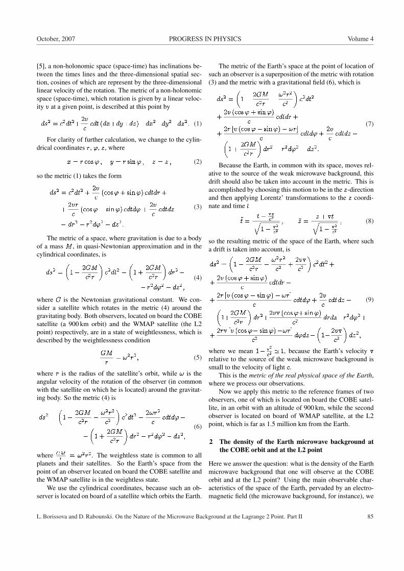
October, 2007 PROGRESS IN PHYSICS Volume 4
[5], a non-holonomic space (space-time) has inclinations be-tween the times lines and the three-dimensional spatial sec-tion, cosines of which are represent by the three-dimensionallinear velocity of the rotation. The metric of a non-holonomicspace (space-time), which rotation is given by a linear veloc-ity v at a given point, is described at this point by
ds2 = c2dt2+2vccdt (dx+dy+dz)�dx2�dy2�dz2: (1)
For clarity of further calculation, we change to the cylin-drical coordinates r, ', z, where
x = r cos' ; y = r sin' ; z = z ; (2)
so the metric (1) takes the form
ds2 = c2dt2 +2vc
(cos'+ sin') cdtdr+
+2vrc
(cos'� sin') cdtd'+2vccdtdz�
� dr2 � r2d'2 � dz2:
(3)
The metric of a space, where gravitation is due to a bodyof a mass M , in quasi-Newtonian approximation and in thecylindrical coordinates, is
ds2 =�
1� 2GMc2r
�c2dt2 �
�1 +
2GMc2r
�dr2�
� r2d'2 � dz2;(4)
where G is the Newtonian gravitational constant. We con-sider a satellite which rotates in the metric (4) around thegravitating body. Both observers, located on board the COBEsatellite (a 900 km orbit) and the WMAP satellite (the L2point) respectively, are in a state of weightlessness, which isdescribed by the weightlessness condition
GMr
= !2r2; (5)
where r is the radius of the satellite’s orbit, while ! is theangular velocity of the rotation of the observer (in commonwith the satellite on which he is located) around the gravitat-ing body. So the metric (4) is
ds2 =�
1� 2GMc2r
� !2r2
c2
�c2dt2 � 2!r2
ccdtd'�
��
1 +2GMc2r
�dr2 � r2d'2 � dz2;
(6)
where GMr = !2r2. The weightless state is common to all
planets and their satellites. So the Earth’s space from thepoint of an observer located on board the COBE satellite andthe WMAP satellite is in the weightless state.
We use the cylindrical coordinates, because such an ob-server is located on board of a satellite which orbits the Earth.
The metric of the Earth’s space at the point of location ofsuch an observer is a superposition of the metric with rotation(3) and the metric with a gravitational field (6), which is
ds2 =�
1� 2GMc2r
� !2r2
c2
�c2dt2 +
+2v (cos'+ sin')
ccdtdr+
+2r [v (cos'� sin')� !r]
ccdtd'+
2vccdtdz�
��
1 +2GMc2r
�dr2 � r2d'2 � dz2:
(7)
Because the Earth, in common with its space, moves rel-ative to the source of the weak microwave background, thisdrift should also be taken into account in the metric. This isaccomplished by choosing this motion to be in the z-directionand then applying Lorentz’ transformations to the z coordi-nate and time t
~t =t+ vz
c2q1� v2
c2
; ~z =z + vtq1� v2
c2
; (8)
so the resulting metric of the space of the Earth, where sucha drift is taken into account, is
ds2 =�
1� 2GMc2r
� !2r2
c2+
2vvc2
�c2dt2 +
+2v (cos'+ sin')
ccdtdr+
+2r [v (cos'� sin')� !r]
ccdtd'+
2vccdtdz�
��
1+2GMc2r
�dr2+
2vv (cos'+ sin')c2
drdz�r2d'2 +
+2rv [v (cos'� sin')�!r]
c2d'dz�
�1� 2vv
c2
�dz2;
(9)
where we mean 1� v2
c2 ' 1, because the Earth’s velocity vrelative to the source of the weak microwave background issmall to the velocity of light c.
This is the metric of the real physical space of the Earth,where we process our observations.
Now we apply this metric to the reference frames of twoobservers, one of which is located on board the COBE satel-lite, in an orbit with an altitude of 900 km, while the secondobserver is located on board of WMAP satellite, at the L2point, which is far as 1.5 million km from the Earth.
2 The density of the Earth microwave background atthe COBE orbit and at the L2 point
Here we answer the question: what is the density of the Earthmicrowave background that one will observe at the COBEorbit and at the L2 point? Using the main observable char-acteristics of the space of the Earth, pervaded by an electro-magnetic field (the microwave background, for instance), we
L. Borissova and D. Rabounski. On the Nature of the Microwave Background at the Lagrange 2 Point. Part II 85

Volume 4 PROGRESS IN PHYSICS October, 2007
derive Einstein’s equations for the space. Einstein’s equationsdescribe the energy and momentum of distributed matter, inthis case the microwave background. So we will know pre-cisely, through Einstein’s equations, the density of the energyof the Earth microwave background which will be observedat the COBE orbit and at the L2 point.
2.1 The Earth space. Its physical properties manifest inobservations of the Earth microwave background
In this particular problem we are interested in the distribu-tion of the Earth microwave background with altitude, givingthe difference in the measurement of the background at theCOBE orbit and at the L2 point. We therefore neglect termslike vv
c2 , which take into account the drift of the whole spaceof the Earth. The quantity 2GM
c2r has its maximum numericalvalue �10�9 at the Earth’s surface, and the value substatiallydecreases with altitude. We therefore neglect the last termsin g11 =� �1+ 2GM
c2r
�, but we do not neglect the last terms in
g00 =1� 2GMc2r � !2r2
c2 , because they will be multiplied by c2later. In such a case the Earth space metric takes the simpli-fied form
ds2 =�
1� 2GMc2r
� !2r2
c2
�c2dt2 +
+2v (cos'+ sin')
ccdtdr+
+2r [v (cos'� sin')� !r]
ccdtd'+
2vccdtdz�
� dr2 � r2d'2 � dz2:
(10)
We will use this metric to determine the density of the en-ergy of the Earth microwave background at the COBE orbitand at the L2 point. We are loooking for the main observ-able characteristics of the space. By the theory of physicalobservable quantities in General Relativity [3, 4], the observ-able properties of a space are determined within the fixedthree-dimensional spatial section of an observer. Those arethe quatities invariant within the spatial section (the so-calledchronometric invariants): the gravitational potential w, thelinear velocity of the space rotation vi, the gravitational iner-tial force Fi, the angular velocity of the space rotation Aik,the three-dimensional metric tensor hik, the space deforma-tionDik, the three-dimensional Christoffel symbols �i
kn, andthe three-dimensional curvature Ciklj . These characteristicscan be calculated through the components of the fundamen-tal metric tensor g�� , which can be easily obtained from aformula for the space metric (see [3, 4] for the details).
The substantially non-zero components of the character-istics of the space of the Earth, calculated though the compo-nents g�� of the metric (10), are
w =GMr
+!2r2
2; (11)
v1 = �v (cos'+ sin')
v2 = �r [v (cos'� sin')� !r]v3 = �v
9>=>; (12)
F1 = (cos'+ sin') vt + !2r � GMr2
F2 = r (cos'� sin') vt ; F3 = vt
9=; (13)
A12 = !r +12�(cos'+ sin') v'�
� r (cos'� sin') vr�
A23 = �v'2; A13 = �vr
2
9>>>>=>>>>; (14)
h11 = h33 = 1 ; h22 = r2; h11 = h33 = 1
h22 =1r2 ; h = r2;
@ lnph
@r=
1r
�122 = �r ; �2
12 =1r
9>>>>=>>>>; (15)
while all components of the tensor of the space deformationDik and the space curvature Ciklj are zero, in the frameworkof our assumptions. Here we assume the plane in cylindri-cal coordinates wherein the space of the Earth rotates: weassume that v doesn’t depend from the z-coordinate. This as-sumption is due to the fact that the Earth, in common withits space, moves relative to a weak (cosmic) microwave back-ground in the direction of its anisotropy. The quantities vr,v', and vt denote the partial derivatives of v by the respectivecoordinates and time.
2.2 Einstein’s equations in the Earth space. The densityof the energy of distributed matter
Einstein’s general covariant equations
R�� � 12g��R = ��T�� + �g�� ; (16)
in a reference frame of the fixed spatial section of an ob-server, are represented by their projections onto the observer’stime line and spatial section [3, 4]. We omit the �-term, thespace deformation Dik, and the space curvature, Ciklj , be-cause they are zero in the framework of our problem. Insuch a case the projected Einstein equations, according toZelmanov [3, 4], are
@F i
@xi+@ lnph
@xiF i � AikAik = ��
2��c2 + U
�@Aik
@xk+@ lnph
@xkAik = ��J i
2AijA�jk� +
12
�@Fi@xk
+@Fk@xi� 2�m
ikFm�
=
=�2��c2hik + 2Uik � Uhik�
9>>>>>>>>>>>>=>>>>>>>>>>>>;(17)
86 L. Borissova and D. Rabounski. On the Nature of the Microwave Background at the Lagrange 2 Point. Part II
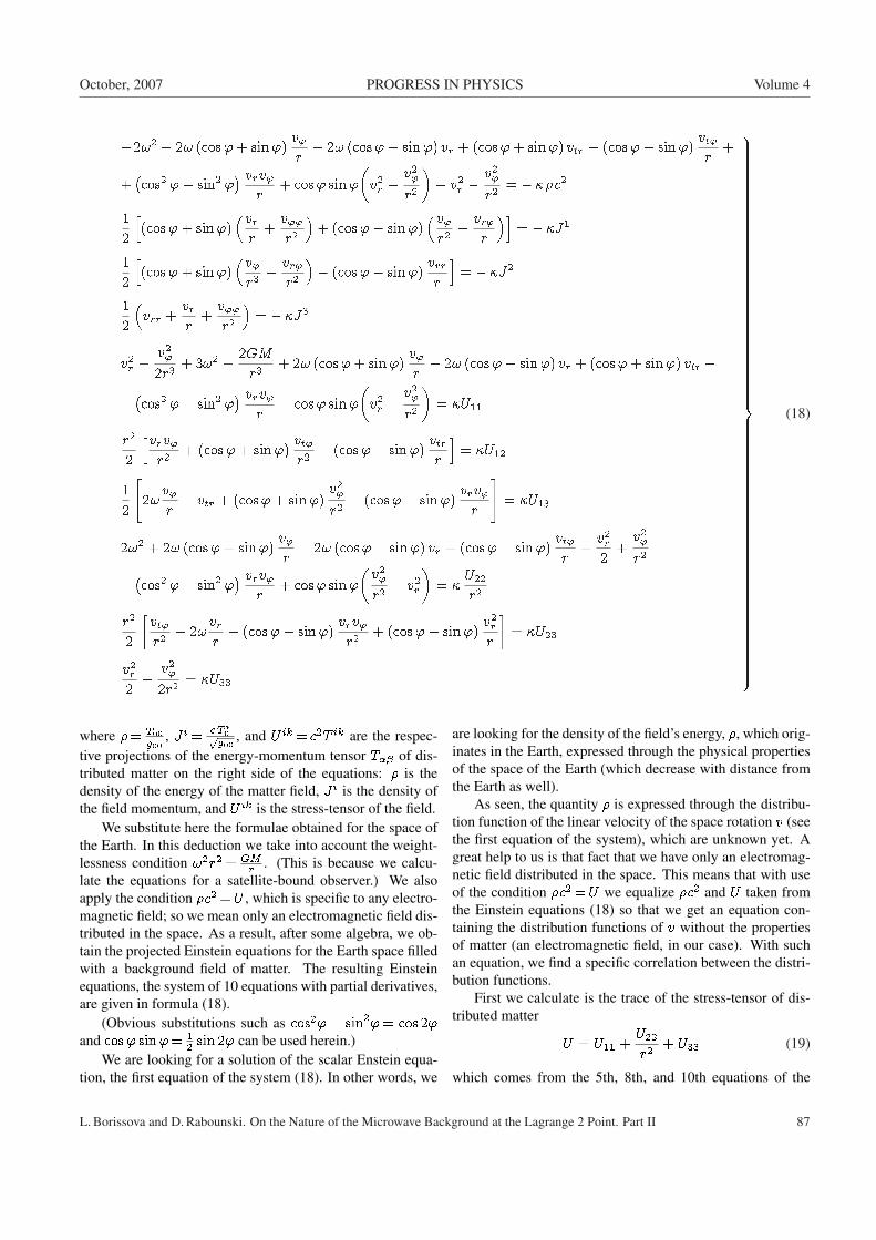
October, 2007 PROGRESS IN PHYSICS Volume 4
�2!2 � 2! (cos'+ sin')v'r
+ 2! (cos'� sin') vr + (cos'+ sin') vtr + (cos'� sin')vt'r
+
+�cos2 '� sin2 '
� vrv'r
+ cos' sin'�v2r � v2
'
r2
�� v2
r � v2'
r2 = ���c212
h(cos'+ sin')
�vrr
+v''r2
�+ (cos'� sin')
�v'r2 � vr'
r
�i= ��J1
12
h(cos'+ sin')
�v'r3 � vr'
r2
�� (cos'� sin')vrrr
i= ��J2
12
�vrr +
vrr
+v''r2
�= ��J3
v2r +
v2'
2r3 + 3!2 +2GMr3 + 2! (cos'+ sin')
v'r� 2! (cos'� sin') vr + (cos'+ sin') vtr �
� �cos2 '� sin2 '� vrv'
r� cos' sin'
�v2r � v2
'
r2
�= �U11
r2
2
hvrv'r2 + (cos'+ sin')
vt'r2 + (cos'� sin')
vtrr
i= �U12
12
"2!v'r
+ vtr + (cos'+ sin')v2'
r2 � (cos'� sin')vrv'r
#= �U13
2!2 + 2! (cos'+ sin')v'r� 2! (cos'� sin') vr + (cos'� sin')
vt'r
+v2r2
+v2'
r2 �� �cos2 '� sin2 '
� vrv'r
+ cos' sin'�v2
'
r2 � v2r
�= �
U22
r2
r2
2
�vt'r2 � 2!
vrr� (cos'+ sin')
vrv'r2 + (cos'� sin')
v2rr
�= �U23
v2r2
+v2'
2r2 = �U33
9>>>>>>>>>>>>>>>>>>>>>>>>>>>>>>>>>>>>>>>>>>>>>>>>>>>>>>>>>=>>>>>>>>>>>>>>>>>>>>>>>>>>>>>>>>>>>>>>>>>>>>>>>>>>>>>>>>>;
(18)
where �= T00g00
, J i = c T i0pg00, and U ik = c2T ik are the respec-
tive projections of the energy-momentum tensor T�� of dis-tributed matter on the right side of the equations: � is thedensity of the energy of the matter field, J i is the density ofthe field momentum, and U ik is the stress-tensor of the field.
We substitute here the formulae obtained for the space ofthe Earth. In this deduction we take into account the weight-lessness condition !2r2 = GM
r . (This is because we calcu-late the equations for a satellite-bound observer.) We alsoapply the condition �c2 =U , which is specific to any electro-magnetic field; so we mean only an electromagnetic field dis-tributed in the space. As a result, after some algebra, we ob-tain the projected Einstein equations for the Earth space filledwith a background field of matter. The resulting Einsteinequations, the system of 10 equations with partial derivatives,are given in formula (18).
(Obvious substitutions such as cos2'� sin2'= cos 2'and cos' sin'= 1
2 sin 2' can be used herein.)We are looking for a solution of the scalar Enstein equa-
tion, the first equation of the system (18). In other words, we
are looking for the density of the field’s energy, �, which orig-inates in the Earth, expressed through the physical propertiesof the space of the Earth (which decrease with distance fromthe Earth as well).
As seen, the quantity � is expressed through the distribu-tion function of the linear velocity of the space rotation v (seethe first equation of the system), which are unknown yet. Agreat help to us is that fact that we have only an electromag-netic field distributed in the space. This means that with useof the condition �c2 =U we equalize �c2 and U taken fromthe Einstein equations (18) so that we get an equation con-taining the distribution functions of v without the propertiesof matter (an electromagnetic field, in our case). With suchan equation, we find a specific correlation between the distri-bution functions.
First we calculate is the trace of the stress-tensor of dis-tributed matter
U = U11 +U22
r2 + U33 (19)
which comes from the 5th, 8th, and 10th equations of the
L. Borissova and D. Rabounski. On the Nature of the Microwave Background at the Lagrange 2 Point. Part II 87
Volume 4 PROGRESS IN PHYSICS October, 2007
(cos'� sin')�vtr'
r� vt'r2
�+ ! (cos'+ sin')
�vr'r� v'r2
�� ! (cos'� sin') vrr + 2vrvrr +v'vr'r2 +
� v2'
r3 + (cos'+ sin') vtrr � 12
cos 2'�v'vrr
r+vrvr'r� vrv'
r2
�+
12
sin 2'�v'vr'r2 � v2
'
r3 � vrvrr�
= 0
(cos'+ sin')�vtr'r2 � vt'
r3
�+ (cos'� sin')
�vt''r3 +
vtrr2
�+ ! (cos'+ sin')
�vrr2 +
v''r3
�+
+! (cos'� sin')�v'r3 � vr'
r2
�+v'v''r4 +
vrvr'r2 +
12
cos 2'�v2
'
r4 � v2rr2 � vrv''
r3 � v'vr'r3
�+
+12
sin 2'�
2vrv'r3 +
v'v''r4 � vrvr'
r2
�= 0
9>>>>>>>>>>>>>>>>>>=>>>>>>>>>>>>>>>>>>;
(24)
Einstein equations (18). We obtain
�U = 4!2 + 4! (cos'+ sin')v'r�
� 4! (cos'� sin') vr + 2v2r +
2v2'
r2 +
+ sin 2'�v2
'
r2 � v2r
�� cos 2'
vrv'r
+
+ (cos'+ sin') vtr + (cos'� sin')vt'r:
(20)
Equalizing it to ��c2 of the first equation of the Einsteinequations (18), we obtain
2!2 + 2! (cos'+ sin')v'r� 2! (cos'� sin') vr +
+ v2r +
v2'
r2 +12
sin 2'�v2
'
r2 � v2r
�� cos 2'
vrv'r
+
+2 (cos'+ sin') vtr + 2 (cos'� sin')vt'r
= 0 :
(21)
Thus we have all physically observable components ofT�� expressed in only the physical observable properties ofthe space. Substituting the components into the conservationlaw for the common field of distributed matter in the space,we look for the formulae of the distribution functions of thespace rotation velocity v.
The conservation law r� T�� = 0, expressed in terms ofthe physical observed quantities�, is [3, 4]
�@�@t
+D�+1c2DijU ij +
+��ri � 1
c2Fi�J i � 1
c2FiJ i = 0
�@Jk@t
+ 2�Dki + A�ki�
�J i +
+��ri � 1
c2Fi�U ik � �F k = 0
9>>>>>>>>>>=>>>>>>>>>>;(22)
�The asterisk denotes the chronometrically invariant differential opera-tors, e.g.
�@@t
= 1pg00
@@t
and�@@xi
= @@xi
+ 1c2vi�@@t
; see [3, 4].
which, under the specific conditions of our problem, become
@J i
@xi+@ lnph
@xiJ i = 0
@Jk
@t+ 2A�ki� J i +
@U ik
@xi+ �k
imUim +
+@ lnph
@xiU ik � �F k = 0
9>>>>>>>=>>>>>>>;(23)
The first, a scalar equation of conservation, meansriJ i= 0, i.e. the flow of the common field of distributedmatter is conserved in the space of the Earth. The second, avector equation of conservation, after substituting the compo-nents of J i and U ik from the Einstein equations (18), and alsoAik (14) and �i
kn (15), give the system (24) of two non-lineardifferential equations with partial derivatives with respect tov (while the third equation vanishes becoming the identity“zero equals zero”).
The exact solution of the system, i.e. a function whichwhen substituted into the equations makes them identities, is
v = T (t) rei'; (25)
where i is the imaginary unit, while T is a function of time(its dimension is sec�1).
Substituting the derivatives
vr = T ei' ; v' = ir T ei' ; vt = _T rei'
vt' = i _T rei'; vtr = T ei'
9=; (26)
into (21), we obtain, after transformations,
Tt (i+ 1) + !T (i� 1)� iT 2
2+ !2 = 0 ; (27)
where _Tt = @T@t . We obtain, for the real part of the equation
_T � !T + !2 = 0 ; (28)
which is a linear differential equation of the first order
_T + f(t)T = g(t) ; (29)
88 L. Borissova and D. Rabounski. On the Nature of the Microwave Background at the Lagrange 2 Point. Part II
October, 2007 PROGRESS IN PHYSICS Volume 4
whose exact solution is
T = e�F�T0 +
Z t
t0=0g(t)eF dt
�; (30)
F (t) =Zf(t)dt : (31)
Substituting f =�!, g=�!2 and integrating the result-ing expression within the limits from t to t0 = 0, we obtainthe solution for the real part of the function T (t):
T (t) = e!t (T0 � !) + ! ; (32)
where T0 is the initial value of T .The imaginary part of the (27) satisfies the differential
equation
Tt + !T � 12T 2 = 0 ; (33)
which is Bernoulli’s equation
Tt + f T 2 + gT = 0 ; (34)
where f =� 12 and g=! are constant coefficients. Such a
Bernoulli equation has the solution
1T
= E(t)Z
fdtE(t)
; E(t) = eRgdt : (35)
Integrating this expression, we obtain
T (t) =2!
1 + Ce!t; (36)
which is the imaginary part of T . Here C is a constant ofintegration. Assuming the initial value t0 = 0, we obtain
C =2!T0� 1 ; (37)
where T0 is the initial value of T . Because, by definitionv=T rei' (25), T has a dimension of sec�1, we consider T0to be the initial frequency of the vibrations of the distributedmatter (background).
So we obtain the final formula for the imaginary part ofthe solution for T :
T (t) =2!T0
T0 + (2! � T0) e!t: (38)
We therefore write the full solution for T as a complexfunction, which is
T (t) = e!t (T0 � !) + ! + i2!T0
(2! � T0) e!t + T0: (39)
We see that the imaginary part of T is zero if T0 = 0.Hence the imaginary part of T originates in the presence ofthe initial non-zero value of T .
Assuming T0 = 0, we obtain: the full solution for T hasonly the real solution
T = !�1� e!t� (40)
when T0 = 0. Substituting this solution into the expression for�c2, i.e. the first equation of the system (18), and taking intoaccount the geometrization condition 21 we have obtained forelectromagnetic field, we obtain the real component of thedensity of the energy, which is
�c2 =3!�
(! � T ) =3!2
��1� �1� e!t�� : (41)
This is the final formula for the observable density ofthe energy W = �c2 of distributed matter in the space of theEarth, where the matter is represented by an electromagneticfield which originates in the Earth, with an additional compo-nent due to the complete rotation of the Earth’s space.
2.3 Calculation of the density of the Earth microwavebackground at the COBE orbit and at the L2 point
We simplify formula (41) according to the assumptions of ourproblem. The quantity !=
pGM�=R3, the frequency of the
rotation of the Earth space for an observer existing in theweightless state, takes its maximum numerical value at theequator of the Earth’s surface, where != 1.24�10�3 sec�1.Obviously, the numerical value of ! decreases with altitudeabove the surface of the Earth. Since ! is a small value, weexpand e!t into the series
e!t � 1 + !t+12!2t2 + : : : (42)
where we omit the higher order terms from consideration. Asa result, we obtain, for the density of the energy of distributedmatter (41) in the space of the Earth (we mean an electromag-netic field originating in the Earth as above),
�c2 =3!2
�; (43)
where !=pGM�=R3. (In derivation of this formula we
neglected the orders of ! higher than !2.) It should be notedthat the quantity ! is derived from the weightless conditionin the space, depending on the mass of the Earth M�, and thedistance R from the centre of the Earth.
Because microwave radiation is related to an electromag-netic field, our theoretical result (43) is applicable to a mi-crowave background originating from the Earth.
Now, with formula (43), we calculate the ratio betweenthe density of the energy of the Earth microwave backgroundat the L2 point (R L2 = 1.5 million km) and at the COBE orbit(R COBE = 6,370 + 900 = 7,270 km)
� L2
�COBE
=R3
COBE
R3L2
' 1.1�10�7: (44)
L. Borissova and D. Rabounski. On the Nature of the Microwave Background at the Lagrange 2 Point. Part II 89

Volume 4 PROGRESS IN PHYSICS October, 2007
At the altitude of a U2 aeroplane (25 km altitude, whichalmost coincides with the location at the Earth’s surface(within the framework of the precision of our calculation),we have RU2 = 6,370 + 25 = 6,395 km. So, we obtain the ra-tio between the density of the Earth microwave background atthe L2 point, at the COBE orbit, and that at the U2 altitude is
� L2
�U2
=R3
U2
R3L2
' 7.8�10�8;�COBE
�U2
=R3
U2
R3COBE
' 0.68: (45)
We see, concerning a microwave background field whichoriginates in the Earth (the Earth microwave background),that a measurement of the background by an absolute instru-ment will give almost the same result at the position of a U2aeroplane and the COBE satellite. However, at the L2 point(as far as 1.5 million km from the Earth, the point of locationof the WMAP satellite and the planned PLANCK satellite),PLANCK, with its ability to function as an absolute instru-ment, should sense only �10�7 of the field registered eitherby the U2 aeroplane or by the COBE satellite.
3 The anisotropy of the Earth microwave backgroundin the COBE orbit and at the L2 point
It is also important to understand what is the anisotropy ofthe Earth microwave background due to a drift of the wholespace of the Earth which would one observe at the COBEorbit and at the L2 point. We solve this problem by usingthe equations of motion of free light-like particles (photons),which are mediators transferring electromagnetic radiation,including those in the microwave region. When treating thephotons which originate in the Earth’s field (the Earth mi-crowave background, for instance), the equations of motionshould manifest an anisotropy in the directions of motion ofthe photon due to the presence of a linear drift in the Earth’sspace as a whole, relative to the source of another field suchas the common field of a compact group of galaxies or thatof the Universe as a whole [1, 2] (a weak microwave back-ground).
The equations of motion of free particles are the geodesicequations.
A light-like free particle, e.g. a free photon, moves alongisotropic geodesic trajectories whose four-dimensional equa-tions are [3, 4]
dK�
d�+ ����K
� dx�
d�= 0 ; (46)
whereK� = cdx�d� is the four-dimensional wave vector of the
photon (the vector satisfies the condition K�K� = 0), while is the proper cyclic frequency of the photon. The three-dimensional observable interval equals the interval of observ-able time d�= cd� along isotropic trajectories, so ds2 == c2d� 2� d�2 = 0. In terms of the physical observable quan-tities, the isotropic geodesic equations are represented by
their projections on the time line and spatial section of anobserver [1, 2]
dd�� c2Fi ci +
c2Dik cick = 0 ;
dd��ci�
+ 2�Dik + A�ik�
�ck�
�F i + �iknc
kcn = 0 ;
9>>>>=>>>>; (47)
where ci = dxid� is the three-dimensional vector of the observ-
able velocity of light (the square of ci satisfies ckck = c2 inthe fixed spatial section of the observer). The first of the equa-tions (the scalar equation) represents the law of energy for theparticle, while the vectorial equation is the three-dimensionalequation of its motion.
We apply the isotropic geodesic equations to the spacemetric (9), which includes a linear drift of the reference spacein the z-direction with a velocity v. Because the dipole-fit velocity of the Earth, extracted from the experimentallyobtained anisotropy of the microwave background, is onlyv = 365�18 km/sec, we neglect the relativistic square in themetric (9) so that it is
ds2 =�
1� 2GMc2r
� !2r2
c2+
2vvc2
�c2dt2 +
+2v (cos'+ sin')
ccdtdr+
+2r [v (cos'� sin')� !r]
ccdtd'+
2vccdtdz�
��
1+2GMc2r
�dr2+
2vv (cos'+ sin')c2
drdz�r2d'2 +
+2rv [v (cos'� sin')�!r]
c2d'dz�
�1� 2vv
c2
�dz2;
(48)
We use the metric with the approximation specific to anobserver located on board the COBE satellite or the WMAPsatellite: the observer exists in the weightless state, so !2r2 == GM
r ; the linear velocity v of the Earth’s space rotationdoesn’t depend on the z-coordinate, the direction of the driftof the whole space. We neglect the terms v2
c2 and also higherorder terms, but retain the term vv
c2 which takes into accountthe drift of the whole space of the Earth: the value of vis determined in the weightless state of the observer; it is'7.9 km/sec close to the surface of the Earth, and hence wehave, near the surface, v
2
c2 � 7�10�10 and vvc2 � 3�10�8. Both
values decrease with distance (altitude) from the Earth’s sur-face, but the term vv
c2 remains two orders higher than v2
c2 . Wealso neglect GMc2r which is �10�9 at the Earth’s surface.
Due to the fact that the terms vvc2 are small corrections in
the metric (48), it is easy to show that the exact solution ofthe conservation equations v=T (t)rei', obtained earlier inthe framework of such a metric without a drift of the whole
90 L. Borissova and D. Rabounski. On the Nature of the Microwave Background at the Lagrange 2 Point. Part II
October, 2007 PROGRESS IN PHYSICS Volume 4
space (10), satisfies the present metric (48) where the drift istaken into account.
Using the solution for T (t) (40), and expanding e!t intoseries e!t� 1 +!t+ : : :, we obtain
T = �!2t ; (49)then
v = �!2trei': (50)
We assume ' to be small. We calculate the observablecharacteristics of the Earth space where the drift of the wholespace is taken into account, i.e. the space of the metric (48).Using the components of the fundamental metric tensor g��taken from the metric (48), we obtain
v1 = !2trei' (cos'+ sin')
v2 = !r2 �!tei' (cos'� sin') + 1�
v3 = !2rtei'
9>>=>>; (51)
F1 = �!2rei' (cos'+ sin') + !2vtei'
F2 = �!2r2ei' (cos'� sin')� i!2rvtei'
F3 = �!2rei'
9>>=>>; (52)
A12 = !r�1 +
!t2
(1� i)�
A23 =i!2trei'
2; A13 =
!2tei'
2
9>>=>>; (53)
h11 = 1 ; h13 =!2vtr (cos'+ sin') ei'
c2
h22 = r2; h23 =!r2v
�!tei' (cos'� sin') +1
�c2
h33 = 1� 2!2vtrei'
c2
h = r2�
1 +2!2vtrei'
c2
�h11 = 1 ; h13 = �!2vtr (cos'+ sin') ei'
c2
h22 =1r2 ; h
23 = �!v�!tei' (cos'� sin') +1
�c2
h33 = 1 +2!2vtrei'
c2
9>>>>>>>>>>>>>>>>>>>>>>>>>=>>>>>>>>>>>>>>>>>>>>>>>>>;
(54)
Because the components h13 and h23 of the tensor hik de-pend on the time coordinate t, we obtain two non-zero com-ponents of the tensor of the space deformation Dik
D13 =!2rv (cos'+ sin') ei'
2c2
D23 =!2r2v (cos'� sin') ei'
2c2
D33 =!2rvei'
c2
9>>>>>>>=>>>>>>>;(55)
the scalar D = hikDik is
D =!2rvei'
c2: (56)
We now calculate the chronometric Christoffel symbolsof the second kind
�122 = �r ; �1
23 =!2rvt (i� 1)
2c2� !rv
c2
�133 =
!2vtei'
c2
�212 =
1r; �2
13 =!2vt (1� i)
2c2r+!vc2r
�233 =
i!2vtei'
c2r
�311 =
!2vt (cos'+ sin') ei'
c2
�312 =
!2rvt (i+ 1) e2i'
2c2; �3
13 = �!2vtei'
c2
�322 =
i!2r2vt (cos'� sin') ei'
c2
�323 =
i!2rvtei'
c2
9>>>>>>>>>>>>>>>>>>>>>>>>>>>>>=>>>>>>>>>>>>>>>>>>>>>>>>>>>>>;
(57)
We use the above characteristics of the Earth’s space towrite the isotropic geodesic equations (47) in componentform. We neglect the terms proportional to 1
c2 in the equa-tions. Besides, in the framework of our asumptions, the dif-ferential with respect to proper time � , i.e.
dd�
=�@@t
+ vi�@@xi
; (58)
can be removed with the regular partial derivative dd� = @
@t .(The starred derivatives become the regular derivatives, andalso the observable velocity of light ci doesn’t depend on thez coordinate in our case where the whole space has a drift inthe z direction.)
The vectorial isotropic geodesic equations, written incomponent notation, are
dc1
d�+2�D1k+A
�1k��ck�F 1+�1
22c2c2 +
+ 2�123c
2c3 + �133c
3c3 = 0
dc2
d�+2�D2k+A
�2k��ck�F 2+2�2
12c1c2 +
+ 2�213c
1c3 + �233c
3c3 = 0
dc3
d�+2�D3k+A
�3k��ck�F 3+�3
11c1c1+2�3
12c1c2 +
+ 2�313c
1c3 + �322c
2c2 + 2�323c
2c3 = 0
9>>>>>>>>>>>>>>=>>>>>>>>>>>>>>;(59)
and after substituting the observable characteristics of thespace, take the form (60–62), where dot denotes differenti-ation with respect to time.
L. Borissova and D. Rabounski. On the Nature of the Microwave Background at the Lagrange 2 Point. Part II 91
Volume 4 PROGRESS IN PHYSICS October, 2007
�r � 2!r�1 +
!t (1� i)2
�_'� !2ei'
�t� vr (cos'+ sin')
c2
�_z + !2�r (cos'+ sin')� vt
�ei'�
� r _'2 +2!rvc2
�!t(i� 1)
2� 1�
_' _z +!2vtei'
c2_z2 = 0 ;
(60)
�'+2!r
�1 +
!t (1� i)2
�_r � !2ei'
r
�it� vr (cos'� sin')
c2
�_z +
!2
r�r (cos'� sin') + ivt
�ei' +
+2r
_r _'� 2!vc2r
�!t(i� 1)
2� 1�
_r _z � i!2vtc2
_z2 = 0 ;(61)
�z + !2ei'�t+
vr (cos'+ sin')c2
�_r + !2rei'
�it+
vr (cos'� sin')c2
�_'+
2!2rvei'
c2_z+
+!2rei' +!2vtei' (cos'+ sin')
c2_r2 +
!2rvt (i+ 1) e2i'
c2_r _'+
2!2vtei'
c2_r _z+
+i!2r2vt (cos'� sin') ei'
c2_'2 +
2i!2rvtei'
c2_' _z = 0;
(62)
_r2 +2!2rvt (cos'+ sin') ei'
c2_r _z + r2 _'2 +
2!r2v�!tei' (cos'� sin') + 1
�c2
_' _z+
+�
1� 2!2rvtei'
c2
�_z2 = c2:
(63)
The space-time interval ds along isotropic geogesics sat-isfies the condition ds2 = 0. This condition, in the terms ofphysical observed quantities, implies constancy of the squareof the three-dimensional observable velocity of light cici ==hik cick = c2 along the trajectory. This condition, for themetric (48), takes the form (63).
A system of the differential equations (60–63) describesthe motion of light-like particles completely, in the givenspace-time of the metric (48).
Earlier in this study we considered only the real partv=T (t)rei' of the solution of the conservation equationsin an electromagnetic field. Because we study the motionof photons in such an electromagnetic field (in the sampleof a microwave background) we only use the real solutionin the system of the equations (60–63). After the functionv=T (t)rei' is substituted into (60–63), we have, after trans-formations, the formulae (64–67) (see Page 93).
We assume that a light-like signal (photon) of the Earthmicrowave radiation moves along the radial direction r. Be-cause the space of the Earth at the location of a satellite (thespace of the weightless state) rotates with an angular veloc-ity ! which depends upon r, we have _'= 0. Two satelliteswhich measure the Earth microwave background are locatedat the altitudes r1 = 900 km and r2 = 1.5 million km respec-tively. Calculation of !2 = GM�
r3 , where M�= 6�1027g isthe mass of the Earth, gives the values: !1 = 10�3 sec�1 and!2 = 3.5�10�6 sec�1. Because both values are small, we usecos'' 1 +!t and sin''!t. Substituting these into thesystem of equations (64–67), and neglecting the terms of or-
der higher than !2 (and also the other higher order terms), weobtain, finally,
�r�!2�t� rv
c2�
_z+!2 (r�vt) +!2vtc2
_z2 = 0 ; (68)
�'+ 2!�
1 +2!t2
�_rr
+!2vc2
_z + 4!2 + 2!_rr
+
+2!v
�1 + !t
2
�c2r
_r _z = 0 ;(69)
�z + !2�t+
rvc2�
_r +2!2vrc2
_z + !2r+
+!2vtc2
_r2 +2!2vtc2
_r _z = 0 ;(70)
_r2 +2!2rvtc2
_r _z +2!2r2vc2
_z+
+�
1� 2!2rvtc2
�_z2 = c2:
(71)
We do choose the coordinate axes so that the z-axis isdirected along the motion of the Earth, in common with itsown electromagnetic field, relative to the source of anotherfeld such as the common feld of a compact group of galaxiesor that of the Universe as a whole (a weak microwave back-ground). We also assume, for simplicity, that the orbit of thesatellite, on board of which an observer is located, lies in theplane orthogonal to the z-direction. In such a case, we have_z0 = 0. We obtain, assuming _z0 = 0,
_r20 = c2; (72)
92 L. Borissova and D. Rabounski. On the Nature of the Microwave Background at the Lagrange 2 Point. Part II
October, 2007 PROGRESS IN PHYSICS Volume 4
�r � !2�t cos'� rv (1 + cos 2'+ sin 2')
c2
�_z � 2!r
�1 +
!t2
�_'+ 2!2r (1 + cos 2'+ sin 2') +
+!2vt cos'� r _'2 � 2!rv�!t
2 + 1�
c2_' _z +
!2vt cos'c2
_z2 = 0 ;(64)
�'+ 2!�
1 +!t2
�_rr
+!2
r
�t sin'+
vr (1 + cos 2'� sin 2')c2
�_z + 2!2 (1 + cos 2'� sin 2') �
� !2
rvt sin'+
2 _r _'r
+2!v
�!t2 + 1
�c2r
_r _z = 0 ;(65)
�z + !2�t cos'+
rv (1 + cos 2'+ sin 2')c2
�_r � 2!2r
�2t sin'� rv (1 + cos 2'� sin 2')
c2
�_'+
+2!2rv cos'
c2_z + !2r cos'+
!2vt (1 + cos 2'+ sin 2')2c2
_r2 +!2vt (cos 2'� sin 2')
c2_r _'+
+2!2vt cos'
c2_r _z +
2!2r2vt (1� cos 2'� sin 2')c2
_'2 � 2!2rvt sin'c2
_' _z = 0 ;
(66)
_r2 +2!2rvt (1 + cos 2'+ sin 2')
c2_r _z + r2 _'2 +
2!r2v�!t
2 (1 + cos 2'� sin 2') +1�
c2_' _z+
+�
1� 2!2rvt cos'c2
�_z2 = c2:
(67)
hence we assume _r' c. So we have r' ct. Substituting theseinto the equation of motion of a photon in the z-direction(70), and taking the weightless condition into account, weobtain the equation of motion in the z direction for a photonassociated with the Earth’s electromagnetic field, the Earthmicrowave background in particular. The equation is
�z +2GM�c2t2
�1 +
vc
�= 0 : (73)
Integrating the equation with the conditions _z0 = 0 andr' ct taken into account, we obtain
_z =2GM�cr
�1 +
vc
�= _z0 + �z0; (74)
where the first term shows that such a photon, initiallylaunched in the r-direction in the rotating space (gravitationalfield) of the Earth, is carried into the z-direction by the rota-tion of the space of the Earth. The second term shows car-riage into the z-direction due to the motion of the Earth inthis direction relative to another source such as a local groupof galaxies or the whole Universe.
Denoting the first term in this formula as _z0= 2GM�cr and
the second term as � _z0= 2GM�vc2r , we obtain the relative car-
riage of the three-dimensional vector of the light velocityfrom the initial r-direction to the z-direction, due to the mo-tion of the Earth, as
� _z0_z0 =
vc: (75)
Such a relative carriage of a photon radiated from theEarth’s surface, applied to the field of photons of the Earth
microwave background radiated in the radial directions, re-veals the anisotropy associated with the dipole component ofthe background.
Such a relative carriage of a photon, associated with theEarth’s electromagnetic field, into the z-direction, doesn’t de-pend on the path travelled by such a photon in the radial di-rection r from the Earth. This means that the anisotropy as-sociated with the dipole component of the Earth microwavebackground shouldn’t be dependent on altitude: it should bethe same be it measured on board a U2 aeroplane (25 km), atthe orbit of the COBE satellite (900 km), and at the L2 point(the WMAP satellite and PLANCK satellite, 1.5 million kmfrom the Earth).
4 Comparing the theoretical results to experimentaldata. Conclusions
We have obtained, from General Relativity, two fundamentalresults:
• A microwave background which originates in the Earth(the EMB) decreases with altitude, such that the den-sity of the energy of this background at the height ofthe COBE satellite (900 km) is just 0.68 times less thatthat at the height of a U2 aeroplane (25 km). The en-ergy of the background at the L2 point (which is up to1.5 million km from the Earth) is only �10�7 that ex-perienced at the location either of a U2 aeroplane or ofthe COBE satellite;
• The anisotropy of the Earth microwave background,
L. Borissova and D. Rabounski. On the Nature of the Microwave Background at the Lagrange 2 Point. Part II 93
Volume 4 PROGRESS IN PHYSICS October, 2007
due to the fast motion of the Earth relative to the sourceof another field, which isn’t connected to the Earth butlocated in depths of the cosmos, does not depend onthe position relative to the Earth’s surface. The dipoleanisotropy is therefore independent of altitude; the an-isotropy will be the same be it measured at the alti-tude of a U2 aeroplane (25 km), the COBE satellite(900 km), or the WMAP satellite located at the L2 point(1.5 million km).
These purely theoretical conclusions, from General Rela-tivity, cause us to consider an Earth origin of the microwavebackground, the monopole 2.7 K component of which wasdiscovered in 1965 by Penzias and Wilson, in a ground-basedobservation [6], while the dipole 3.35 mK component wasfirst observed in 1969 by Conklin, also via a ground-based ob-servation [7], then studied by Henry [8], Corey [9], and alsoSmoot, Gorenstein, and Muller, who organized a stratosphereobservation on board a U2 aeroplane [11]. (See the history ofthe observations in detail in Lineweaver’s paper [10].)
There are many problems in the observation of the mi-crowave background. The monopole component, at low fre-quencies, is easy to observe at the Earth’s surface [6]. Thedipole component is best observed at the altitude of a U2aeroplane [11], at the altitude of 900 km (the COBE satellite)and also at 1.5 million km (the WMAP satellite located at theL2 point) where its anisotropy is clearly indicated [12–17].Conversely, the monopole observed on Earth and in COBEorbit, has yet to be recorded at the L2 point: the WMAP satel-lite has only differential instruments on board, which are ableto indicate only the anisotropy of the background, not its ab-solute value.
On the other hand, as shown by Robitaille [18–22], sucha phenomenology of the observations has a clear explanationas an Earth microwave background which originates not in acosmic source, but the oceans of the Earth, which produce mi-crowave signals, in particular, with an apparent temperatureof 2.7 K. Besides, as pointed out in [21, 23], the observedanisotropy of the microwave background can be explained asa relativistic effect of the motion of the observer, in commonwith the source of the background (the Earth), relative to thesource of a noise microwave field, which has no specific tem-perature, and a source of which is located in depths of thecosmos (i.e. the distance from the many sources).
According to our theory, which supports the phenomenol-ogy of the Earth microwave background, proposed by Ro-bitaille [18–22], we have four new specific terms, namely:
1. The EMB (the Earth Microwave Background);2. The EMBM (the monopole associated with the Earth
Microwave Background);3. The EMBD (the dipole associated with the Earth Mi-
crowave Background);4. The EMBA (the anisotropy of the Earth Microwave
Background, associated with the dipole).
The PLANCK satellite (which has an absolute instrumenton board), will soon be launched to the L2 point, on 31stJuly 2008, and should find an experimental verification ofour theory.
Acknowledgement
We are very grateful to Pierre-Marie Robitaille for consulta-tions and valuable comments. We also are thankful to DelyanZhelyazov for a few typing mistakes found in the formulaewhen this issue was sent to print.
Submitted on August 29, 2007 / Accepted on September 06, 2007First published online on September 08, 2007
Online version corrected on February 11, 2008
References
1. Borissova L. Preferred spatial directions in the Universe:a General Relativity approach. Progress in Physics, 2006, v. 4,51–58.
2. Borissova L. Preferred spatial directions in the Universe. Part II.Matter distributed along orbital trajectories, and energy pro-duced from it. Progress in Physics, 2006, v. 4, 59–64.
3. Zelmanov A. L. Chronometric invariants and co-moving coor-dinates in the general relativity theory. Doklady Acad. NaukUSSR, 1956, v.107(6), 815–818.
4. Zelmanov A. L. Chronometric invariants. American ResearchPress, Rehoboth (NM), 2006.
5. Schouten J. A. und Struik D. J. Einfuhrung in die neuren Meth-oden der Differentialgeometrie. Noordhoff, Groningen, 1938.
6. Penzias A. A. and Wilson R. W. A measurement of excess an-tenna temperature at 4080 Mc/s. Astrophys. J., 1965, v. 1, 419–421.
7. Conklin E. K. Velocity of the Earth with respect to the CosmicBackground Radiation. Nature, 1969, v. 222, 971.
8. Henry P. S. Isotropy of the 3 K Background. Nature, 1971,v. 231, 516–518.
9. Corey B. E. and Wilkinson D. T. A measurement of the CosmicMicrowave Background Anisotropy at 19 GHz. Bulletin of theAmerican Astronomical Society, 1976, v. 8, 351.
10. Lineweaver C.H. The CMB Dipole: The most recent measure-ment and some history. In Microwave Background Anistropies.Proceedings of the XVIth Moriond Astrophysics Meeting, LesArcs, Savoie, France, March 16th-23rd, 1996, F. R. Bouchet,R. Gispert, B. Guilderdoni, and J.T.T. Van, eds., Gif-sur-Yvette:Editions Frontieres, 1997; (see also arXiv: astro-ph/9609034).
11. Smoot G. F., Gorenstein M. V. and Muller R. A. Detection ofanisotropy in the Cosmic Blackbody Radiation. Phys. Rev.Lett., 1977, v. 39, 898–901.
12. Boggess N.W., et al. The COBE mission: its design and per-fomance two years after launch. Astrophys. J., 1992, v. 397,420–429.
13. Fixsen D.J., et al. The Cosmic Microwave Background spec-trum from the full COBE FIRAS data set. Astrophys. J., 1996,v. 473, 576–587.
94 L. Borissova and D. Rabounski. On the Nature of the Microwave Background at the Lagrange 2 Point. Part II
October, 2007 PROGRESS IN PHYSICS Volume 4
14. Smoot G.F., et al. Preliminary results from the COBE diffe-rential microwave interferometers: large angular scale isotropyof the Cosmic Microwave Background. Astrophys. J., 1991,v. 371, L1–L5.
15. Page L., et al. The optical design and characterization of theMicrowave Anisotropy Probe. Astrophys. J., 2003, v. 585, 566–586.
16. Bennett C.L., et al. The Microwave Anisotropy Probe mission.Astrophys. J., 2003, v. 583(1), 1–23.
17. Bennett C.L., et al. First-year Wilkinson Microwave AnisotropyProbe (WMAP) observations: preliminary maps and basic re-sults. Astrophys. J. Suppl. Ser., 2003, v. 148(1), 1–27.
18. Robitaille P.-M. WMAP: a radiological analysis. Progress inPhysics, 2007, v. 1, 3–18.
19. Robitaille P.-M. On the origins of the CMB: insight from theCOBE, WMAP and Relikt-1 satellites. Progress in Physics,2007, v. 1, 19–23.
20. Robitaille P.-M. On the Earth Microwave Background: absorp-tion and scattering by the atmosphere. Progress in Physics,2007, v. 3, 3–4.
21. Robitaille P.-M. and Rabounski D. COBE and the absolute as-signment of the CMB to the Earth. 2007 APS March Meet-ing, Denver, Colorado, Monday–Friday, March 5–9, 2007,http://meetings.aps.org/link/BAPS.2007.MAR.L20.7
22. Robitaille P.-M. On the nature of the microwave background atthe Lagrange 2 Point. Part I. Progress in Physics, 2007, v. 4,74–83.
23. Rabounski D. The relativistic effect of the deviation be-tween the CMB temperatures obtained by the COBE satellite.Progress in Physics, 2007, v. 1, 19–21.
L. Borissova and D. Rabounski. On the Nature of the Microwave Background at the Lagrange 2 Point. Part II 95
Volume 4 PROGRESS IN PHYSICS October, 2007
A New Conformal Theory of Semi-Classical Quantum General Relativity
Indranu Suhendro
Department of Physics, Karlstad University, Karlstad 651 88, SwedenE-mail: spherical [email protected]
We consider a new four-dimensional formulation of semi-classical quantum general rel-ativity in which the classical space-time manifold, whose intrinsic geometric propertiesgive rise to the effects of gravitation, is allowed to evolve microscopically by means ofa conformal function which is assumed to depend on some quantum mechanical wavefunction. As a result, the theory presented here produces a unified field theory of grav-itation and (microscopic) electromagnetism in a somewhat simple, effective manner.In the process, it is seen that electromagnetism is actually an emergent quantum fieldoriginating in some kind of stochastic smooth extension (evolution) of the gravitationalfield in the general theory of relativity.
1 Introduction
We shall show that the introduction of an external parameter,the Planck displacement vector field, that deforms (“maps”)the standard general relativistic space-time S1 into an evolvedspace-time S2 yields a theory of general relativity whosespace-time structure obeys the semi-classical quantum me-chanical law of evolution. In addition, an “already quan-tized” electromagnetic field arises from our schematic evolu-tion process and automatically appears as an intrinsic geomet-ric object in the space-time S2. In the process of evolution, itis seen that from the point of view of the classical space-timeS1 alone, an external deformation takes place, since, by defi-nition, the Planck constant does not belong to its structure. Inother words, relative to S1, the Planck constant is an externalparameter. However from the global point of view of the uni-versal (enveloping) evolution space M4, the Planck constantis intrinsic to itself and therefore defines the dynamical evo-lution of S1 into S2. In this sense, a point in M4 is not strictlysingle-valued. Rather, a point in M4 has a “dimension” de-pending on the Planck length. Therefore, it belongs to boththe space-time S1 and the space-time S2.
2 Construction of a four-dimensional metric-compatibleevolution manifold M4
We first consider the notion of a four-dimensional, universalenveloping manifoldM4 with coordinates x� endowed with amicroscopic deformation structure represented by an exteriorvector field � (x� ) which maps the enveloped space-timemanifold S1 2M4 at a certain initial point P0 onto a new en-veloped space-time manifold S2 2M4 at a certain point P1through the diffeomorphism
x� (P1) = x� (P0) + l ��;
where l=q
G ~c3 � 10�33 cm is the Planck length expressed
in terms of the Newtonian gravitational constantG, the Dirac-
Planck constant ~, and the speed of light in vacuum c, in sucha way that
�� = l ��
lim~!0
�� = 0 :
From its diffeomorphic structure, we therefore see thatM4 is a kind of strain space. In general, the space-time S2evolves from the space-time S1 through the non-linear map-ping
P (�) : S1 ! S2 :
Note that the exterior vector field � can be expressed as�=��h� = ���g� (the Einstein summation convention is em-ployed throughout this work) where h� and g� are the sets ofbasis vectors of the space-times S1 and S2, respectively (like-wise for �). We remark that S1 and S2 are both endowed withmetricity through their immersion in M4, which we shall nowcall the evolution manifold. Then, the two sets of basis vec-tors are related by
g� =���� + lr� ���h�
or, alternatively, by
g� = h� + l� �r� ���
�g�
where ��� are the components of the Kronecker delta.At this point, we have defined the two covariant deriva-
tives with respect to the connections ! of S1 and � of S2 asfollows:
r�A��:::��::: = @�A��:::��::: + !���A
��:::��::: + !���!��:::��::: + : : :
�!���A��:::��::: � !���A��:::��::: � : : :and
�r�B��:::��::: = @�B��:::��::: + ����B
��:::��::: + ����B����::: + : : :
�����B��:::��::: � ����B
��:::��::: � : : :
for arbitrary tensor fields A and B, respectively. Here@� = @=@ x�, as usual. The two covariant derivatives aboveare equal only in the limit ~! 0.
96 I. Suhendro. A New Conformal Theory of Semi-Classical Quantum General Relativity
October, 2007 PROGRESS IN PHYSICS Volume 4
Furthermore, we assume that the connections ! and � aregenerally asymmetric, and can be decomposed into their sym-metric and anti-symmetric parts, respectively, as
!��� =�h�; @vh�
�= !�(��) + !�[��]
and���� =
�g�; @vg�
�= ��(��) + ��[��]:
Here, by (a; b) we shall mean the inner product betweenthe arbitrary vector fields a and b.
Furthermore, by direct calculation we obtain the relation
@�g� =�!��� + l
�r����!��� + l @��r�����h� :
Hence, setting
F��� = !��� + l�(r���)!��� + @�
�r����� =
= !���+ l�(r���)!���+@�@���+��@�!���+ (@���)!���
�we may simply write
@�g� = F���h� :
Meanwhile, we also have the following inverse relation:
h� =���� � l �r� ���
�g� :
Hence we obtain
@�g� =�!��� + l (r���)!��� + l @�@��� +
+ l ��@�!��� + l (@���)!��� � l !��� �r� ����� l (r���)!��� �r� ��� � l (@v@���) �r� ����� l �� �@�!���� �r� ��� �l (@���)!��� �r� ���
�g� :
Using the relation @�g� = ����g� (similarly, @�h� ==!���h�), we obtain the relation between the two connec-tions � and ! as follows:
���� = !��� + l�(r���)!��� + @�@��� +
+ ��@�!��� (@���)!����!��� �r� ���� (r���)!��� �r� ����� (@�@���) �r� ������ �@�!���� �r� ��� � (@���)!��� �r� ���
�which is a general non-linear relation in the components ofthe exterior displacement field �. We may now write
���� = F��� +G���
where, recalling the previous definition of F ��� , it can be re-written as
F ��� = !��� + l��@�!��� + !���!���
��� +
+ @�@��� + (@���)!��� + (@���)!����
and where
G��� = �l �!��� + l�(r���) !���
+ @�@��� + �� @�!��� + (@� ��) !����� �r� ��� :
At this point, the intrinsic curvature tensors of the space-times S1 and S2 are respectively given by
K���� = 2
�h�; @[�@�]h�
�=
= @�!��� � @� !��� + !��� !��� � !��� !���and
R���� = 2�g�; @[�@�]g�
�=
= @����� � @����� + ���� ���� � �������� :
We may also define the following quantities built from theconnections !��� and ���� :
D���� = @�!��� + @�!��� + !��� !
��� + !���!
���
and
E���� = @����� + @����� + ���� ���� + ��������
from which we may define two additional “curvatures”X andP by
X���� = (h�; @�@�h�) =
12�K�
��� +D�����
=
= @�!��� + !���!���and
P ���� = (g�; @�@� g�) =12�R���� + E����
�=
= @����� + ���� ����
such that K���� = 2X�
�[��] and R���� = 2P ��[��].Now, we see that
F �(��) = !�(��) + l�
12D�
��� �� + @�@���
�+
+ l�(@���) !��� + (@���) !���
�and
F�[��] = !�[��] +12lK�
��� �� :
In addition, we also have
G�(��) = l�!�(��) + l
�12D�
��� �� + @�@���
���r� ��� +
+ l�l�
(@���) !��� + (@���) !����� �r� ���
and
G�[��] = l�!�[��] � 1
2lK�
��� ���
�r� ���:
Now, the metric tensor g of the space-time S1 and themetric tensor h of the space-time S2 are respectively given by
h�� = (h�; h�)
andg�� = (g�; g�)
I. Suhendro. A New Conformal Theory of Semi-Classical Quantum General Relativity 97

Volume 4 PROGRESS IN PHYSICS October, 2007
where the following relations hold:
h��h�� = ���g��g�� = ���
In general, the two conditions h�� g�� , ��� andg�� h��,��� must be fulfilled unless l=0 (in the limit ~!0).Furthermore, we have the metricity conditions
r� h�� = 0 ;and �r� g�� = 0 :
However, note that in general, �r� h�� , 0 andr�g�� , 0.Hence, it is straightforward to see that in general, the met-
ric tensor g is related to the metric tensor h by
g�� = h�� + 2 lr(���) + l2r���r���which in the linear approximation reads
g�� = h�� + 2 lr(���) :
The formal structure of our underlying geometric frame-work clearly implies that the same structure holds in n di-mensions as well.
3 The conformal theory
We are now in the position to extract a physical theory ofquantum gravity from the geometric framework in the pre-ceding section by considering the following linear conformalmapping:
g� = e'h�
where the continuously differentiable scalar function ' (x�)is the generator of the quantum displacement field in the evo-lution space M4 and therefore connects the two space-timesS1 and S2.
Now, for reasons that will be apparent soon, we shall de-fine the generator ' in terms of the canonical quantum me-chanical wave function (x�) as
' = ln (1 +M )12
whereM = �1
2l�im0c~
�2:
Here m0 is the rest mass of the electron. Note that thesign � signifies the signature of the space-time used.
Now, we also have the following relations:
g� = e�'h�;h� = e�'g�;h� = e'g�;
(g�; g�) = (h�; h�) = ��� ;
(g�; h�) = e2'��� ;
(h�; g�) = e�2'��� ;
as well as the conformal transformation
g�� = e2'h�� :Hence
g�� = e�2' h�� :
We immediately see that
g�� h�� = e2' ��� ;
h�� g�� = e�2' ��� :
At this point, we see that the world-line of the space-timeS2, s=
Rph�� dx�dx� , is connected to that of the space-
time S1, �=Rp
g�� dx�dx� , through
ds = e2'd� :
Furthermore, from the relation
g� =���� + lr��� �h� = e'h�
we obtain the important relation
lr��� = (e' � 1)h�� ;which means that
��� = lr��� = ��� ;
i.e., the quantum displacement gradient tensor field � is sym-metric. Hence we may simply call � the quantum strain ten-sor field. We also see that the components of the quantumdisplacement field, �� = l ��, can now be described by thewave function as
�� = l @� i.e.,
= 0 +1l
Z��dx�
for an arbitrary initial value 0 (which, most conveniently,can be chosen to be 0).
Furthermore, we note that the integrability condition��� = ��� means that the space-time S1 must now possessa symmetric, linear connection, i.e.,
!��� = !��� =12h�� (@�h�� � @�h�� + @�h��) ;
which are just the Christoffel symbols f ��� g in the space-timeS1. Hence ! is now none other than the symmetric Levi-Civita (Riemannian) connection. Using the metricity condi-tion @�g�� = ���� + ����, i.e.,
@� g�� = Mh�� @� + (1 +M ) (!��� + !���) ;
we obtain the mixed form
!��� =12
(1 +M )�1 (@�g�� � @�g�� + @�g��)�� 1
2M (1 +M )�1 (h��@� � h��@� + h��@� )
98 I. Suhendro. A New Conformal Theory of Semi-Classical Quantum General Relativity
October, 2007 PROGRESS IN PHYSICS Volume 4
i.e.,
!��� =12
(1 +M )�1 h�� (@�g�� � @� g�� + @� g��)�� 1
2M (1 +M )�1 ����@� + ��� @� � h��h��@� � :
It may be noted that we have used the customary conven-tion in which ���� = g�� ���� and !��� =h��!
��� .
Now we shall see why we have made the particular choice'= ln (1 +M )
12 . In order to explicitly show that it now
possess a stochastic part, let us rewrite the components of themetric tensor of the space-time S2 as
g�� = (1 +M )h�� :
Combining this relation with the linearized relationg�� =h��+ 2 lr(� ��) and contracting the resulting relation,we obtain
lD2 = 2�e2' � 1
�= 2M ;
where we have defined the differential operator D2 == h��r�r� such that
D2 = h���@�@� � !��� @� � :
ExpressingM explicitly, we obtainD2 = � �m0 c~
�2 ,i.e., �
D2 � �m0c~
�2� = 0
which is precisely the Klein-Gordon equation in the presenceof gravitation.
We may note that, had we combined the relation g�� == (1 +M )h�� with the fully non-linear relation
g�� = h�� + 2 lr(���) + l2r���r��� ;we would have obtained the following non-linear Klein-Gordon equation:�D2 � �m0 c
~
�2� = l2h��h�� (r�r� ) (r�r� ) :
Now, from the general relation between the connections �and ! given in Section 2, we obtain the following importantrelation:
��[��] = �12l���� � l �r� ���
�K�
�����;
which not only connects the torsion of the space-time S2 withthe curvature of the space-time S1, but also describes the tor-sion as an intrinsic (geometric) quantum phenomenon. Notethat
K���� = @�
����
�� @�
����
�+
+����
�����
������
�����
�are now the components of the Riemann-Christoffel curvaturetensor describing the curvature of space-time in the standard
general relativity theory.Furthermore, using the relation between the two sets of
basis vectors g� and h�, it is easy to see that the connection� is semi-symmetric as
���� = !��� + ��� @�'
or, written somewhat more explicitly,
���� =12h�� (@�h�� � @�h�� + @�h��) +
+12��� @�
�ln (1 +M )
�:
We immediately obtain
��(��) = !��� +12����@�'+ ��� @�'
�and
��[��] =12����@�'� ��� @�'� :
Additionally, using the relation
!��� = !��� = @��
lnp
det (h)�
=
= @��
ln�e�'
pdet (g)
��= @�
�lnp
det (g)�� @�'
we may now define two semi-vectors by the following con-tractions:
�� = ���� = @��
lnp
det (h)�
+ 4 @�'
�� = ���� = @��
lnp
det (h)�
+ @�'
or, written somewhat more explicitly,
�� = @��
lnp
det (h) + ln (1 +M )2�
�� = @��
lnp
det (h) + lnp
1 +M �:
We now define the torsion vector by
�� = ��[��] =32@�' :
In other words,
�� =34
M(1 +M )
@� :
Furthermore, it is easy to show that the curvature tensorsof our two space-times S1 and S2 are now identical:
R���� = K����
which is another way of saying that the conformal transfor-mation g� = e' h� leaves the curvature tensor of the space-time S1 invariant. As an immediate consequence, we obtainthe ordinary expression
R���� =12
(@�@�h��+@�@�h���@�@�h���@�@�h��) +
+h���!���!
��� � !��� !���� :
I. Suhendro. A New Conformal Theory of Semi-Classical Quantum General Relativity 99
Volume 4 PROGRESS IN PHYSICS October, 2007
Hence the following cyclic symmetry in Riemannian ge-ometry:
R���� +R���� +R���� = 0
is preserved in the presence of torsion. In addition, besidesthe obvious symmetry R���� =�R����, we also have thesymmetry
R���� = �R����which is due to the metricity condition of the space-times S1and S2. This implies the vanishing of the so-called Homoth-etic curvature as
H�� = R���� = 0 :
The Weyl tensor is given in the usual manner by
C���� = R���� � 12
(h��R�� + h��R����h��R�� � h��R��)� 1
6(h��h�� � h��h��)R ;
where R�� =R���� are the components of the symmetricRicci tensor and R=R�� is the Ricci scalar.
Now, by means of the conformal relation g�� = e2' h��we obtain the expression
R���� = e�2'�@�@�g�� + @�@�g�� � @�@�g��@�@�g�� +
+ g���
�������� � ���������
+ (@�g�� � @�g��) @�'+
+ (@�g�� � @�g��) @�'+ (@� g�� � @�g��) @�'+
+ (@�g�� � @�g��) @�'+ g��@�@�'+ g��@�@�'+
� g��@�@�'� g��@�@�'+ 2 (g��@�'@�'+
+ g��@�'@�'� g��@�'@�'� g��@�'@�'�+
+ g����
����@�'�����@�'�����
�����@�'�����@�'
������:
Note that despite the fact that the curvature tensor of thespace-time S2 is identical to that of the space-time S1 andthat both curvature tensors share common algebraic symme-tries, the Bianchi identity in S2 is not the same as the ordinaryBianchi identity in the torsion-free space-time S1. Instead, wehave the following generalized Bianchi identity:
�r�R���� + �r�R���� + �r�R���� =
= 2�
��[��]R���� + ��[��]R���� + ��[��]R�����:
Contracting the above relation, we obtain
�r��R�� � 1
2g��R
�= 2 g����[��]R
�� + ��[��]R
���� :
Combining the two generalized Bianchi identities abovewith the relation ��[��] = 1
2
���� @�'� ��� @�' �, as well as re-
calling the definition of the torsion vector, and taking intoaccount the symmetry of the Ricci tensor, we obtain
�r�R���� + �r�R���� + �r�R���� =
= 2 (R����@�'+R����@�'+R����@� ')
and
�r��R�� � 1
2g��R
�= � 2
�R�� � 1
2g��R
�@�'
which, upon recalling the definition of the torsion vector, maybe expressed as
�r��R�� � 1
2g��R
�= � 4
3
�R�� � 1
2g��R
��� :
Apart from the above generalized identities, we may alsogive the ordinary Bianchi identities as
r�R���� +r�R���� +r�R���� = 0
andr��R�� � 1
2h��R
�= 0 :
4 The electromagnetic sector of the conformal theory.The fundamental equations of motion
Based on the results obtained in the preceding section, let usnow take the generator ' as describing the (quantum) electro-magnetic field. Then, consequently, the space-time S1 is un-derstood as being devoid of electromagnetic interaction. Aswe will see, in our present theory, it is the quantum evolutionof the gravitational field that gives rise to electromagnetism.In this sense, the electromagnetic field is but an emergentquantum phenomenon in the evolution space M4.
Whereas the space-time S1 is purely gravitational, theevolved space-time S2 does contain an electromagnetic field.In our present theory, for reasonsthat will be clear soon, weshall define the electromagnetic field F 2S2 2M4 in terms ofthe torsion of the space-time S2 by
F�� = 2m0c2
�e��[��]u� ;
where �e is the (elementary) charge of the electron and
u� = g��dx�
ds= e2'h��
dx�
dsare the covariant components of the tangent velocity vectorfield satisfying umu u� = 1.
We have seen that the space-time S2 possesses a manifestquantum structure through its evolution from the purely grav-itational space-time S1. This means that �e may be defined interms of the fundamental Planck charge e as follows:
�e = Ne = Np
4�"0~c ;
where N is a positive constant and "0 is the permitivity offree space. Further investigation shows that N =
p� where
��1� 137 is the conventional fine structure constant.Let us now proceed to show that the geodesic equation of
motion in the space-time S2 gives the (generalized) Lorentzequation of motion for the electron. The result of parallel-
100 I. Suhendro. A New Conformal Theory of Semi-Classical Quantum General Relativity
October, 2007 PROGRESS IN PHYSICS Volume 4
transferring the velocity vector field u along the world-line(in the direction of motion of the electron) yields
�Du�
ds=� �r�u��u� = 0 ;
i.e., du�
ds+ ����u
�u� = 0 ;
where, in general,
���� =12g�� (@�g�� � @�g�� + @�g��) + ��[��]�
� g�� �g����[��] + g�� ��[��]
�:
Recalling our expression for the components of the tor-sion tensor in the preceding section, we obtain
���� =12g�� (@�g�� � @�g�� + @�g��) +
+ g��g��@�'� ��� @�'which is completely equivalent to the previously obtained re-lation
���� = !��� + ��� @�' :Note that
���� =
12g�� (@�g�� � @�g�� + @�g��)
are the Christoffel symbols in the space-time S2. These arenot to be confused with the Christoffel symbols in the space-time S1 given by !��� .
Furthermore, we havedu�
ds+ ��
�� u�u� = 2g����[��]u�u
�:
Now, since we have set F�� = 2m0 c2�e ��[��]u�, we obtain
the equation of motion
m0c2�du�
ds+ ��
��u�u�
�= �eF�� u
� ;
which is none other than the Lorentz equation of motion forthe electron in the presence of gravitation. Hence, it turns outthat the electromagnetic field, which is non-existent in thespace-time S1, is an intrinsic geometric object in the space-time S2. In other words, the space-time structure of S2 inher-ently contains both gravitation and electromagnetism.
Now, we see that
F�� =m0c2
�e(u�@�'� u�@�') :
In other words,
�eF�� u� = m0c2
�u�d'ds� g��@�'
�:
Consequently, we can rewrite the electron’s equation ofmotion as
du�
ds+ ��
��u�u� = u�
d'ds� g�� @�' :
We may therefore define an asymmetric fundamental ten-sor of the gravoelectromagnetic manifold S2 by
~g�� = g��d'ds� �em0c2
F��
satisfying~g��u� = @�' :
It follows immediately that����d'ds� �em0c2
F��
�u� = g�� @�'
which, when expressed in terms of the wave function , givesthe Schrodinger-like equation
u�d ds
=1M
�@�'+
�em0c2
F��u�� :
We may now proceed to show that the electromagneticcurrent density given by the covariant expression
j� = � c4�
�r�F��is conserved in the present theory.
Let us first call the following expression for the covariantcomponents of the electromagnetic field tensor in terms of thecovariant components of the canonical electromagnetic four-potential A:
F�� = �r�A� � �r�A�such that �e �r�A� =m0c2u�@�', i.e.,
m0c2@�' = �e u� �r�A�which directly gives the equation of motion
m0c2d'ds
= �e u�u� �r�A� :Hence, we obtain the following equation of state:
m0c2d ds
= 2 �e(1 +M )
Mu�u� �r�A� :
Another alternative expression for the electromagneticfield tensor is given by
F�� = @�A� � @�A�2��[��]A� =
= @�A� � @�A� + A� @�'� A�@�' :In the particular case in which the field-lines of the elec-
tromagnetic four-potential propagate in the direction of theelectron’s motion, we have
F�� = ��e�
1� �2
c2
� (@�u� � @�u�)
where � is a proportionality constant and �=� �eq
�m0
.Then, we may define a vortical velocity field, i.e., a spin field,through the vorticity tensor which is given by
!�� =12
(@�u� � @�u�)
I. Suhendro. A New Conformal Theory of Semi-Classical Quantum General Relativity 101
Volume 4 PROGRESS IN PHYSICS October, 2007
and henceF�� = 2�
�e�1� �2
c2
� !�� ;which describes an electrically charged spinning region in thespace-time continuum S2.
Furthermore, we have the following generalized identityfor the electromagnetic field tensor:
�r�F�� + �r�F�� + �r�F�� =
= 2�
��[��]F�� + ��[��]F�� + ��[��]F���
which, in the present theory, takes the particular form
�r�F�� + �r�F�� + �r�F�� =
= 2 (F��@�'+ F��@�'+ F��@�') :
Contracting, we have
�r� j� = � c4�
�r��
��[��]F���:
We therefore expect that the expression in the bracketsindeed vanishes. For this purpose, we may set
j� = � c4�
��[��] F��
and hence, again, using the relation
��[��] =12����@�'� ��� @�'� ;
we immediately see that
�r�j� � c4�
�@�' �r�F�� + F��
�@�@�'� ��[��]@�'
��=
= � j� @�'� c4�
��[��]F�� @�'
i.e.,�r� j� = 0 :
At this point, we may note the following: the fact thatour theory employs torsion, from which the electromagneticfield is extracted, and at the same time guarantees electromag-netic charge conservation (in the form of the above continuityequation) in a natural manner is a remarkable property.
Now, let us call the relation
��[��] = �12l���� � l �r� ���
�R���� �
�
obtained in Section 3 of this work (in which R���� =K����).
This can simply be written as
��[��] = �12le�'R���� ��
i.e.,
��[��] = �12le�'R���� g��@� :
Hence, we obtain the elegant result
F�� = � l m0c2
�ee�'R���� u� g��@�
i.e.,
F�� = � l�e
m0c2p1 +M
R���� u� g��@�
or, in terms of the components of the (dimensionless) micro-scopic displacement field �,
F�� = � l m0c2
�ee�'R���� u� g����
which further reveals how the electromagnetic field originatesin the gravitational field in the space-time S2 as a quantumfield. Hence, at last, we see a complete picture of the elec-tromagnetic field as an emergent phenomenon. This com-pletes the long-cherished hypothesis that the electromagneticfield itself is caused by a massive charged particle, i.e., whenm0 = 0 neither gravity nor electromagnetism can exist. Fi-nally, with this result at hand, we obtain the following equa-tion of motion for the electron in the gravitational field:
du�
ds+ ��
��u�u� = � le�'R���� u� ��u�
i.e.,
du�
ds+ ��
��u�u� = � lp
1 +M R���� u�u
� @� :
In addition, we note that the torsion tensor is now seen tobe given by
�� = �12le�'R�� ��
or, alternatively,
�� = �12le�'R�� g��@� :
In other words,
�� = �12
lp1 +M
R�� g��@� :
Hence, the second generalized Bianchi identity finallytakes the somewhat more transparent form
�r��R�� � 1
2g��R
�=
= �23le�'
�R��R�� � 1
2RR��
�g�� @�
i.e.,
�r��R�� � 1
2g��R
�=
= �23
lp1 +M
�R��R�� � 1
2RR��
�g�� @� :
102 I. Suhendro. A New Conformal Theory of Semi-Classical Quantum General Relativity
October, 2007 PROGRESS IN PHYSICS Volume 4
5 Final remarks
The present theory, in its current form, is still in an elementarystate of development. However, as we have seen, the emer-gence of the electromagnetic field from the quantum evolu-tion of the gravitational field is a remarkable achievementwhich deserves special attention. On another occasion, weshall expect to expound the structure of the generalized Ein-stein’s equation in the present theory with a generally non-conservative energy-momentum tensor given by
T�� = � c4
8�G
�R�� � 1
2g��R
�which, like in the case of self-creation cosmology, seems toallow us to attribute the creation and annihilation of matterdirectly to the scalar generator of the quantum evolution pro-cess, and hence the wave function alone, as
�r�T�� = �23
lp1 +M
T��R�� g�� @� , 0 :
6 Acknowledgements
The author is dearly indebted to Dmitri Rabounski and Ste-phen J. Crothers for their continuous support and sincere as-sistance.
Submitted on August 23, 2007Accepted on September 24, 2007
References
1. Thiemann T. Introduction to Modern Canonical Quantum Gen-eral Relativity. arXiv: gr-qc/0110034.
2. Barber G. A. The principles of self-creation cosmology and itscomparison with General Relativity. arXiv: gr-qc/0212111.
3. Brans C. H. Consistency of field equations in “self-creation”cosmologies. Gen. Rel. Grav., 1987, v. 19, 949–952.
I. Suhendro. A New Conformal Theory of Semi-Classical Quantum General Relativity 103

Volume 4 PROGRESS IN PHYSICS October, 2007
Joint Wave-Particle Properties of the Individual Photon
Bo Lehnert
Alfven Laboratory, Royal Institute of Technology, S-10044 Stockholm, SwedenE-mail: [email protected]
Two-slit experiments performed earlier by Tsuchiya et al. and recently by Afshar etal. demonstrate the joint wave-particle properties of the single indiviual photon, andagree with Einstein’s argument against Complementarity. These results cannot be ex-plained by conventional theory in which Maxwell’s equations serve as a guiding line andbasis. On the other hand a revised quantum electrodynamic theory based on a nonzeroelectric field divergence in the vacuum yields results which appear to be consistent withthe experiments. A model of the individual photon is thus deduced from the theory, inthe form of a wave packet behaving as a single entity and having simultaneous waveand particle properties.
1 Introduction
Ever since the earlier epoch of natural science, the wave-particle duality of light has appeared as something of anenigma. In Bohr’s principle of Complementarity, this dualityhas been a cornerstone in the interpretation of quantum me-chanics. Thereby the wavelike and particlelike properties areconceived to be complementary, in the sense that they are mu-tually exclusive, and no experiment can reveal both at once.This formulation of quantum mechanics has been successfulin many applications and is widely accepted by physicists, butit is full of apparent paradoxes which made Einstein deeplyuncomfortable [1].
During the latest decades additional investigations on thenature of light have been made, among which the two-slit ex-periments by Tsuchiya et al. [2] and Afshar et al. [3] deserveparticular attention. These investigations verify that there is ajoint wave-particle duality of the individual photon, thus be-ing in agreement with Einstein’s argument against Comple-mentarity.
In this paper part of the results by Tsuchiya et al. andAfshar et al. are reviewed and compared with a revised quan-tum electrodynamic theory by the author. The latter theoryis based on a vacuum state that is not merely an empty spacebut includes the electromagnetic fluctuations of the zero pointenergy and a corresponding nonzero electric charge densityassociated with a nonzero electric field divergence. A shortdescription of the theory is presented, whereas its detaileddeductions are given elsewhere [4–7].
2 The two-slit experiments
A photon-counting imaging system has earlier been elabo-rated by Tsuchiya et al. [2] and incorporates the ability todetect individual photons, spatial resolution, and the capabil-ity of real-time imaging and subsequent image analysis. Twoparallel slits of size 50�m � 4 mm at a spacing of 250�m
were arranged to pass light through an interference filter ata wavelength of 253.7 nm. The full size of the obtained im-age on the monitor screen of the experiment was 11.4 mmat the input plane. Since the purpose of the investigationwas to demonstrate the interference property of a single pho-ton itself, the spacing of individual photons was made muchlonger than their coherence time, so that interference betweenindividual photons could be prevented. For this reason, neu-tral density filters were used to realize a very low lightlevel, where the counting rates were of the order of 100per second.
As the measurements started, bright very small dots ap-peared at random positions on the monitor screen. After 10seconds had elapsed, a photon-counting image was seen onthe screen, containing 103 events, but its overall shape wasnot yet clearly defined. After 10 minutes, however, the totalaccumulated counts were 6�104, and an interference patternformed by the dots was clearly detected. The diameter ofeach dot was of the order of 6�10�3 of the screen size, andthe fringe distance about 5�10�2 of it. The effect of closingone of the double slits was finally observed. Then the inter-ference pattern did not appear, but a diffraction pattern wasobserved.
As concluded by Tsuchiya et al., these results cannot beexplained by mutually exclusive wave and particle descrip-tions of the photon, but give a clear indication of the wave-particle duality of the single individual photon [2].
These important results appear not to have attracted thewide interest which they ought to deserve. However, as longas 22 years later, Afshar et al. [3] conducted a two-slit ex-periment based on a different methodology but with a similaroutcome and conclusions. In this investigation there was asimultaneous determination of the wave and particle aspectsof light in a “welcher-weg” experiment, beyond the limita-tions set by Bohr’s principle of Complementarity. The ex-periment included a pair of pinholes with diameters of 40 nmand center-to-center separation of 250�m, with light from a
104 Bo Lehnert. Joint Wave-Particle Properties of the Individual Photon
October, 2007 PROGRESS IN PHYSICS Volume 4
diode laser of the wavelength 638 nm. These parameter val-ues were thus not too far from those of the experiments byTsuchiya et al. In addition, six thin wires of 127�m diameterwere placed at a distance of 0.55 m from the pinholes, and atthe minima of the observed interference pattern. When thispattern was present, the disturbance to the incoming beam bythe wire grid was minimal. On the other hand, when the inter-ference pattern was absent, the wire grid obstructed the beam.Also here the investigation was conducted in the low photonflux regime, to preclude loss of which-way information dueto the intrinsic indistinguishability of coherent multi-photonsystems. When the flux was 3�104 photons per second, theaverage separation between successive photons was estimatedto about 10 km. The experiments were performed in fourways, i.e. with both pinholes open in absence of the wire grid,with both pinholes open in presence of the wire grid, and witheither pinhole open in presence of the same grid.
From the measured data the which-way information andthe visibility of an interference pattern could then be deter-mined within the same experimental setup. The which-wayinformation thus indicates through which pinhole the parti-clelike photon has passed. At the same time the interferenceindicates that the same wavelike photon must have sampledboth pinholes so that an interference pattern could be formed.These derived properties of the individual photon refer backto the same space-time event, i.e. to the moment when thesingle photon passed the plane of the pinholes.
Consequently, also these experimental results force us toagree vith Einstein’s argument against Complementarity [3].
3 Shortcomings of conventional theory
In conventional quantum electrodynamics (QED), Maxwell’sequations have served as a guiding line and basis when thereis a vacuum state with a vanishing electric charge density anda zero electric field divergence [8]. According to Schiff [8]and Heitler [9] the Poynting vector then defines the momen-tum of the pure radiation field, expressed by sets of quan-tized plane waves. As pointed out by Feynman [10], thereare nevertheless unsolved problems which lead to difficultieswith Maxwell’s equations that are not removed by and notdirectly associated with quantum mechanics. Consequently,QED will also become subject to the shortcomings of the con-ventional field theory.
To be more specific in connection with a theoretical modelof the individual photon, we start here with the following gen-eral physical requirements to be fulfilled:
• The model should have the form of a wave or a wavepacket of preserved and limited geometrical shape,propagating with undamped motion in a defined direc-tion of three-space. This leads to an analysis in a cylin-drical frame (r; '; z) with z in the direction of propa-gation;
• The obtained general solutions for the field quantitiesshould extend all over space, and no artificial bound-aries would have to be introduced in the vacuum;
• The integrated total field energy should remain finite;• The solutions should result in an angular momentum
(spin) of the photon as a propagating boson particle.
Maxwell’s equations in the vacuum state yield solutionsfor any field quantity Q having the normal mode form
Q = Q(r) exp�i (�!t+ �m'+ kz)
�(1)
in cylindrical geometry where ! is the frequency and k and �mare the wave numbers with respect to the z and ' directions.We further introduce
K20 =
�!c
�2 � k2: (2)
When K20 > 0 the phase velocity becomes larger and the
group velocity smaller than the velocity c of light. The gen-eral solution then has field components in terms of Besselfunctions Z �m(K0 r) of the first and second kind, where ther-dependence of every component is of the form Z �m=r orZ �m+1 [11]. Application to a photon model then leads to thefollowing results:
• Already the purely axisymmetric case �m= 0 results ina Poynting vector which yields zero spin;
• The spin also vanishes when K0 = 0 and the phase andgroup velocities both are equal to c;
• There is no clearly defined spatial limitation of the so-lutions;
• With no material boundaries such as walls, the total in-tegrated field energy becomes divergent.
Consequently, conventional theory based on Maxwell’sequations in the vacuum state does not lead to a physicallyrelevant model for the individual photon.
4 Photon physics in revised quantum electrodynamics
An extended electromagnetic theory applied to the vacuumstate and aiming beyond Maxwell’s equations serves asa guiding line and basis of the present theoretical approach[4–7]. In four-dimensional representation the theory has thefollowing form�
1c2@2
@t2�r2
�A� = �0J� ; � = 1; 2; 3; 4 ; (3)
where A� are the electromagnetic potentials. As deducedfrom the requirement of Lorentz invariance, the four-currentdensity of the right-hand member of equation (3) becomes
J� = (j; ic��) = "0(div E) (C; ic) ; C 2 = c2 (4)
with c as the velocity of light, E denoting the electric fieldstrength, and SI units being adopted. Further B= curl A is
Bo Lehnert. Joint Wave-Particle Properties of the Individual Photon 105
Volume 4 PROGRESS IN PHYSICS October, 2007
the magnetic field strength derived from the three-space mag-netic vector potential A. In equation (4) the velocity vector Chas the modulus c. Maxwell’s equations in the vacuum are re-covered when div E = 0, whereas div E, 0 leads to a space-charge current density (4) in the vacuum. The correspondingthree-space part j = "0(div E)C appears in addition to thedisplacement current.
The revised basic field equations of dynamic states in athree-dimensional representation are now given by the waveequation�
@2
@t2� c2r2
�E +
�c2r+ C
@@t
�(div E) = 0 (5)
for the electric field, and the equation
curl E = � @B@t
(6)
of electromagnetic induction. The characteristic features ofthe field equations (3)–(6) are as follows:
• The theory is based on the pure radiation field in thevacuum state, including contributions from a nonzeroelectric charge density;
• The associated nonzero electric field divergence intro-duces an additional degree of freedom, leading to newsolutions and new physical phenomena. This also be-comes important in situations where this divergence ap-pears to be small;
• The theory is both Lorentz and gauge invariant;
• The velocity of light is no longer a scalar c but a vectorC with the modulus c.
To become complete, the theory has to be quantized. Inabsence as well as in presence of source terms, such as theright-hand member of equation (3), the quantized field equa-tions are generally equivalent to the original field equationsin which all field quantities are replaced by their expectationvalues, as shown by Heitler [9]. As a first step and a simplifi-cation, the general solutions of the field equations will there-fore first be determined, and relevant quantum conditions willafterwards be imposed on these solutions. This is justified bythe expectation values due to Heitler. The present theory maytherefore not be too far from the truth, in the sense that it rep-resents the most probable states in a first approximation to arigorous quantum-theoretical deduction.
4.1 Application to a model of the individual photon
The theory of equations (3)–(6) is now applied to the model ofan individual photon in the axisymmetric case where@=@'= 0 in a cylindrical frame (r; '; z) with z along the di-rection of propagation. Screw-shaped modes where @=@', 0end in several respects up with similar results, but becomemore involved and have been described elsewhere [6, 7].
The velocity vector of equation (4) is in this axisymmetriccase given by
C = c (0; cos�; sin�) (7)
where � is a constant angle, and cos� and sin� could inprinciple have either sign but are here limited to positive val-ues for the sake of simplicity. The form (7) can be shownto imply that the electromagnetic energy has one part whichpropagates in the z-direction, and another part which circu-lates in the '-direction around the axis of symmetry and be-comes associated with the spin [6, 7]. Normal modes of theform (1) with �m= 0 then result in general solutions for thecomponents of E and B, being given in terms of differentialexpressions of a generating function
F = G0R(�) exp�i(�!t+ kz)
�: (8)
(HereG0 is an amplitude factor, �= r=r0, and r0 represents acharacteristic radius of the geometrical configuration in ques-tion.) The corresponding dispersion relation becomes
! = kv ; v = c (sin�) (9)
thus resulting in axial phase and group velocities, both be-ing equal to v < c . Not to get into conflict with the experi-ments by Michelson and Morley, the condition 0< cos�� 1has to be imposed on the parameter cos�. As an example,cos�6 10�4 would make the velocity v differ from c by lessthan the eight decimal in the value of c. As a consequenceof the dispersion relation (9) with v < c and of the detaileddeductions, the total integrated field energy mc2 further be-comes equivalent to a total mass m and a rest mass
m0 = mp
1� (v=c)2 = m (cos�): (10)
This rest mass is associated with the angular momentumwhich only becomes nonzero for a nonzero electric field di-vergence. When div E, cos�, and m0 vanish, we are thusback to the conventional case of Section 3 with its spinlessand physically irrelevant basis for a photon model. Even ifthe electric field divergence at a first glance appears to be asmall quantity, it thus has a profound effect on the physics ofan individual photon model.
From the obtained general solutions it has further beenshown that the total integrated charge and magnetic momentvanish, whereas the total integrated mass m and angular mo-mentum s remain nonzero.
From the solutions of the normal wave modes, a wavepacket has to be formed. In accordance with experimental ex-perience, such a packet should have a narrow line width. Itsspectrum of wave numbers k should then be piled up around amain wave number k0 and a corresponding wavelength�0 = 2�=k0. The effective axial length 2z0 of the packet isthen much larger than �0.
To close the system, two relevant quantum conditionshave further to be imposed. The first concerns the total in-tegrated field energy, in the sense that mc2 =h�0 according
106 Bo Lehnert. Joint Wave-Particle Properties of the Individual Photon
October, 2007 PROGRESS IN PHYSICS Volume 4
to Einstein and Planck, where the frequency �0 � c=�0, forcos�� 1. The second condition is imposed on the total in-tegrated angular momentum which should become equal tos=h=2� for the photon to behave as a boson particle.
From combination with the wave packet solutions, the im-posed quantum conditions result in expressions for an effec-tive transverse diameter 2 r of the wave packet. In respect tothe radial part R of the generating function (8), there are twoalternatives which are both given by
2 r ="�0
� (cos�)(11)
and become specified as follows:• When "= 1 expression (11) stands for a part R(�)
which is convergent at the origin �= 0. This resultsin an effective photon diameter being only moderatelysmall, but still becoming large as compared to atomicdimensions;
• When "� 1 there are solutions for a part R(�) whichis divergent at �= 0. Then finite field quantities canstill be obtained within a whole range of small ", inthe limit of a shrinking characteristic radius r0 = c0 "where c0 is a positive constant having the dimension oflength. This alternative results in an an effective pho-ton diameter which can become very small, such as torealize a state of “needle radiation” first proposed byEinstein. Then the diameter (11) can become compara-ble to atomic dimensions.
It is thus seen that the requirements on a photon model canbe fulfilled by the present revised theory. Its wave packet so-lutions have joint wave-particle properties. In some respectsthis appears to be similar to the earlier wave-particle dualityoutlined by de Broglie, where there is a “pilot wave” prop-agating along the axis, on which wave a “particle-like” partis “surfing”. However, such a subdivision is not necessary inthe present case where the wave packet behaves as one singleentity, having wave and particle properties at the same time.
Attention is finally called to a comparison between thedefinition of the momentum of the pure radiation field interms of the Poynting vector on one hand, and that given bythe expression p =�i~r in the deduction of the Schrodingerequation for a particle with mass on the other [5]. For nor-mal modes the axial component of p becomes pz = ~k asexpected. However, in the transverse direction of a photonmodel being spatially limited and having a finite effective di-ameter (11), there would arise a nonzero transverse momen-tum pr as well, but this appears to be physically unacceptablefor a photon model.
4.2 The present photon model and its relation to two-slitexperiments
The limits of the effective photon diameter (11) can be es-timated by assuming an upper limit of 2 r when "= 1 and
cos�= 10�4, and a lower limit of 2 r when "= cos�. Thenthe effective diameter would be in the range of the values�0=� 6 2r 6 104�0=�, but the lower limit could even be lowerwhen "< cos� for strongly pronounced needle radiation.From this first order estimate, and from the features of thetheory, the following points should be noticed:
• The diameter of the dot-shaped marks on the monitorscreen of the experiment by Tsuchiya et al. is of theorder of 6�10�3 of the screen size, i.e. about 10�4 m.With the wave length �0 = 253.7 nm, the effective pho-ton diameter would then be in the range of the values7�10�4 > 2 r > 7�10�8 m. This range covers the ob-served size of the dots;
• The width of the parallel slits in the experiments byTsuchiya et al. is 5�10�5 m and their separation dis-tance is 25�10�5 m. The corresponding pinhole diam-eters and their center-to-center separation in the exper-iments by Afshar et al. are 4�10�5 m and 25�10�5 m,respectively, and the wavelength is �0 = 638 nm. In thelatter experiments the effective diameter is estimated tobe in the range 2�10�7 6 2 r 6 2�10�3 m. In both ex-periments the estimated ranges of 2 r are thus seen tocover the slit widths and separation distances;
• A large variation of a small cos� has only a limited ef-fect on the phase and group velocities of equation (9).Also a considerable variation of a small " does not in-fluence the general deductions of the theory [4, 6, 7]even if it ends up with a substantial change of the di-ameter (11). This leads to the somewhat speculativequestion whether the state of the compound parameter"=cos� could adopt different values during the propa-gation of the wave packet. This could then be relatedto “photon oscillations” as proposed for a model witha nonzero rest mass, in analogy with neutrino oscilla-tions [4, 7];
• As compared to the slit widths and the separation dis-tances, the obtained ranges of 2 r become consistentwith the statement by Afshar et al. that the same wave-like photon can sample both pinholes to form an inter-ference pattern;
• Interference between cylindrical waves should takeplace in a similar way as between plane waves. In par-ticular, this becomes obvious at the minima of the in-terference pattern where full cancellation takes place;
• Due to the requirement of a narrow line width, the wavepacket length 2z0 by far exceeds the wave length �0and the effective diameter 2 r. Therefore the packetforms a very long and narrow wave train;
• Causality raises the question how the photon can“know” to form the interference pattern on the monitorscreen already when it passes the slits. An answer maybe provided by the front part of the elongated packet
Bo Lehnert. Joint Wave-Particle Properties of the Individual Photon 107
Volume 4 PROGRESS IN PHYSICS October, 2007
which may serve as a “precursor”, thereby also rep-resenting the quantum mechanical wave nature of thepacket. Alternatively, there may exist a counterpart tothe precursor phenomenon earlier discussed by Stratton[11] for conventional electromagnetic waves.
5 Conclusions
The two-slit experiments by Tsuchiya et al. and by Afshar etal. demonstrate the joint wave-particle properties of the in-dividual photon, and agree with Einstein’s argument againstComplementarity. These experiments cannot be explained byconventional theory. The present revised theory appears onthe other hand to become consistent with the experiments.
Submitted on September 17, 2007Accepted on September 24, 2007
References
1. Merali Z. Free will — you only think you have it. New Scientist,6 May 2006, p. 8–9.
2. Tsuchiya T., Inuzuka E., Kurono T., Hosoda M. Photon-counting imaging and its applications. Advances in Electronicsand Electron Physics, 1985, v. 64A, 21–31.
3. Afshar S. S., Flores E., McDonald K. F., Knoesel E. Paradoxin wave-particle duality. Foundations of Physics, 2007, v. 37,295–305.
4. Lehnert B. Photon physics of revised electromagnetics.Progress in Physics, 2006, v. 2, 78–85.
5. Lehnert B. Momentum of the pure radiation field. Progress inPhysics, 2007, v. 1, 27–30.
6. Lehnert B. Revised quantum electrodynamics with fundamen-tal applications. In: Proceedings of 2007 ICTP Summer Col-lege on Plasma Physics (Edited by P. K. Shukla, L. Stenflo, andB. Eliasson), World Scientific Publishers, Singapore, 2008.
7. Lehnert B. A revised electromagnetic theory with funda-mental applications. Swedish Physics Archive (Edited byD. Rabounski), The National Library of Sweden, Stockholm,2007; and Bogoljubov Institute for Theoretical Physics (Editedby A. Zagorodny), Kiev, 2007.
8. Schiff L. I. Quantum Mechanics. McGraw-Hill BookComp. Inc., New York, 1949, Chs. XIV, IV, and II.
9. Heitler W. The quantum theory of radiation. Third edition.Clarendon Press, Oxford, 1954, Ch. II and Appendix.
10. Feynman R. P. Lectures on physics: mainly eletromagnetismand matter. Addison-Wesley, Reading, Massachusetts, 1964.
11. Stratton J. A. Electromagnetic theory. McGraw-Hill BookComp. Inc., New York and London, 1941, Ch. VI, Sec. 5.18.
108 Bo Lehnert. Joint Wave-Particle Properties of the Individual Photon
October, 2007 PROGRESS IN PHYSICS Volume 4
A New Derivation of Biquaternion Schrodinger Equationand Plausible Implications
Vic Christianto� and Florentin Smarandachey�Sciprint.org — a Free Scientific Electronic Preprint Server, http://www.sciprint.org
E-mail: [email protected] of Mathematics, University of New Mexico, Gallup, NM 87301, USA
E-mail: [email protected]
In the preceding article we argue that biquaternionic extension of Klein-Gordon equa-tion has solution containing imaginary part, which differs appreciably from known so-lution of KGE. In the present article we discuss some possible interpretation of thisimaginary part of the solution of biquaternionic KGE (BQKGE); thereafter we offer anew derivation of biquaternion Schrodinger equation using this method. Further obser-vation is of course recommended in order to refute or verify this proposition.
1 Introduction
There were some attempts in literature to generalise Schro-dinger equation using quaternion and biquaternion numbers.Because quaternion number use in Quantum Mechanics hasoften been described [1, 2, 3, 4], we only mention in this paperthe use of biquaternion number. Sapogin [5] was the first tointroduce biquaternion to extend Schrodinger equation, whileKravchenko [4] use biquaternion number to describe neat linkbetween Schrodinger equation and Riccati equation.
In the present article we discuss a new derivation of bi-quaternion Schrodinger equation using a method used in thepreceding paper. Because the previous method has been usedfor Klein-Gordon equation [1], now it seems natural to ex-tend it to Schrodinger equation. This biquaternion effect maybe useful in particular to explore new effects in the context oflow-energy reaction (LENR) [6]. Nonetheless, further obser-vation is of course recommended in order to refute or verifythis proposition.
2 Some interpretations of preceding result of biquater-nionic KGE
In our preceding paper [1], we argue that it is possible towrite biquaternionic extension of Klein-Gordon equation asfollows��
@2
@t2�r2
�+i�@2
@t2�r2
��'(x; t)=�m2'(x; t): (1)
Or this equation can be rewritten as�}�}+m2�'(x; t) = 0 (2)
provided we use this definition
}=rq+irq =��i @
@t+e1
@@x
+e2@@y
+e3@@z
�+
+ i��i @
@T+ e1
@@X
+ e2@@Y
+ e3@@Z
� (3)
where e1, e2, e3 are quaternion imaginary units obeying(with ordinary quaternion symbols: e1 = i, e2 = j, e3 = k)
i2 = j2 = k2 = �1 ; ij = �ji = k ;
jk = �kj = i ; ki = �ik = j ;(4)
and quaternion Nabla operator is defined as [7]
rq = �i @@t
+ e1@@x
+ e2@@y
+ e3@@z
: (5)
Note that equation (3) and (5) included partial time-differentiation.
It is worth nothing here that equation (2) yields solutioncontaining imaginary part, which differs appreciably fromknown solution of KGE:
y(x; t) =�
14� i
4
�m2t2 + constant: (6)
Some possible alternative interpretations of this imagina-ry part of the solution of biquaternionic KGE (BQKGE) are:
(a) The imaginary part implies that there is exponentialterm of the wave solution, which is quite similar tothe Ginzburg-Landau extension of London phenomen-ology [8]
(r) = j (r)j ei'(r) ; (7)
because (6) can be rewritten (approximately) as:
y(x; t) =ei
4m2t2; (8)
(b) The aforementioned exponential term of the solution(8) can be interpreted as signature of vortices solution.Interestingly Navier-Stokes equation which impliesvorticity equation can also be rewritten in terms ofYukawa equation [3];
(c) The imaginary part implies that there is spiral wave,which suggests spiralling motion of meson or other par-ticles. Interestingly it has been argued that one can ex-plain electron phenomena by assuming spiralling elec-
V. Christianto and F. Smarandache. A New Derivation of Biquaternion Schrodinger Equation and Plausible Implications 109
Volume 4 PROGRESS IN PHYSICS October, 2007
trons [9]. Alternatively this spiralling wave may al-ready be known in the form of Bierkeland flow. Formeson observation, this could be interpreted as anotherform of meson, which may be called “supersymmetric-meson” [1];
(d) The imaginary part of solution of BQKGE also impliesthat it consists of standard solution of KGE [1], andits alteration because of imaginary differential operator.That would mean the resulting wave is composed oftwo complementary waves;
(e) Considering some recent proposals suggesting thatneutrino can have imaginary mass [10], the aforemen-tioned imaginary part of solution of BQKGE can alsoimply that the (supersymmetric-) meson may be com-posed of neutrino(s). This new proposition may requirenew thinking both on the nature of neutrino and alsosupersymmetric-meson [11].
While some of these propositions remain to be seen, inderiving the preceding BQKGE we follow Dirac’s phrase that“One can generalize his physics by generalizing his mathe-matics”. More specifically, we focus on using a “theorem”from this principle, i.e.: “One can generalize his mathemat-ics by generalizing his (differential) operator”.
3 Extended biquaternion Schrodinger equation
One can expect to use the same method described above togeneralize the standard Schrodinger equation [12]�
� ~2
2m�u+ V (x)
�u = Eu ; (9)
or, in simplified form, [12, p.11]:
(�� + wk)fk = 0 ; k = 0; 1; 2; 3: (10)
In order to generalize equation (9) to biquaternion version(BQSE), we use first quaternion Nabla operator (5), and bynoticing that � � rr, we get
� ~2
2m
�rq �rq +
@2
@t2
�u+
�V (x)� E�u = 0 : (11)
Note that we shall introduce the second term in order to‘neutralize’ the partial time-differentiation ofrq �rq operator.
To get biquaternion form of equation (11) we can use ourdefinition in equation (3) rather than (5), so we get
� ~2
2m
�}�}+
@2
@t2� i @2
@T 2
�u+
�V (x)�E�u = 0 : (12)
This is an alternative version of biquaternionic Schrodin-ger equation, compared to Sapogin’s [5] or Kravchenko’s [4]method. We also note here that the route to quaternionizeSchrodinger equation here is rather different from what is de-scribed by Horwitz [13, p. 6]
~H = e1E ; (13)
or~H q = q
�q�1 e1 q
�E ; (14)
where the quaternion number q, can be expressed as follows(see [13, p. 6] and [4])
q = q0 +3Xi=1
qi ei : (15)
Nonetheless, further observation is of course recommend-ed in order to refute or verify this proposition (12).
4 Numerical solution of biquaternion Schrodingerequation
It can be shown that numerical solution (using Maxima [14])of biquaternionic extension of Schrodinger equation yieldsdifferent result compared to the standard Schrodinger equa-tion, as follows. For clarity, all solutions were computed in1-D only.
For standard Schrodinger equation [12], one can rewriteequation (9) as follows:
(a) For V (x) > E:
� ~2
2m�u+ a � u = 0 ; (16)
(b) For V (x) < E:
� ~2
2m�u� a � u = 0 : (17)
Numerical solution of equation (16) and (17) is given (byassuming ~=1 and m= 1=2 for convenience)
(%i44) -’diff (y, x, 2) + a*y;(%o44) a � y � d2
d2xy
(a) For V (x) > E:
(%i46) ode2 (%o44, y, x);(%o46) y = k1 � exp(
pa � x) + k2 � exp(�pax)
(b) For V (x) < E:
(%i45) ode2 (%o44, y, x);(%o45) y = k1 � sinh(
pa � x) + k2 � cosh(
pa � x)
In the meantime, numerical solution of equation (12), isgiven (by assuming ~=1 and m= 1=2 for convenience)
(a) For V (x) > E:
(%i38) (%i+1)*’diff (y, x, 2) + a*y;
(%o38) (i+ 1) d2
d2xy + a � y
(%i39) ode2 (%o38, y, x);(%o39) y = k1 � sin(
p ai+1 � x) + k2 � cos(
p ai+1 � x)
(b) For V (x) < E:
(%i40) (%i+1)*’diff (y, x, 2) - a*y;
(%o40) (i+ 1) d2
d2xy � a � y
(%i41) ode2 (%o40, y, x);(%o41)y = k1 � sin(
p� ai+1 � x) + k2 � cos(
p� ai+1 � x)
110 V. Christianto and F. Smarandache. A New Derivation of Biquaternion Schrodinger Equation and Plausible Implications
October, 2007 PROGRESS IN PHYSICS Volume 4
Therefore, we conclude that numerical solution of bi-quaternionic extension of Schrodinger equation yields differ-ent result compared to the solution of standard Schrodingerequation. Nonetheless, we recommend further observation inorder to refute or verify this proposition/numerical solutionof biquaternion extension of spatial-differential operator ofSchrodinger equation.
As side remark, it is interesting to note here that if weintroduce imaginary number in equation (16) and equation(17), the numerical solutions will be quite different comparedto solution of equation (16) and (17), as follows
� i~2
2m�u+ au = 0 ; (18)
where V (x) > E, or
� i~2
2m�u� au = 0 ; (19)
where V (x) < E.Numerical solution of equation (18) and (19) is given (by
assuming ~=1 and m= 1=2 for convenience)
(a) For V (x) > E:
(%i47) -%i*’diff (y, x, 2) + a*y;(%o47) a � y � i d2
d2xy
(%i48) ode2 (%o47, y, x);(%o48) y = k1 � sin(
pia � x) + k2 � cos(
pia � x)
(b) For V (x) < E:
(%i50) -%i*’diff (y, x, 2) - a*y;(%o50) �a � y � i d2
d2xy
(%i51) ode2 (%o50, y, x);(%o51) y = k1 � sin(�pia � x) + k2 � cos(�pia � x)
It shall be clear therefore that using different sign for dif-ferential operator yields quite different results.
Acknowledgement
Special thanks to Prof. Diego Rapoport who mentionedSprossig’s interesting paper [3]. VC would like to dedicatethis article for RFF.
Submitted on September 24, 2007Accepted on September 26, 2007
References
1. Yefremov A., Smarandache F. and Christianto V. Yang-Millsfield from quaternion space geometry, and its Klein-Gordonrepresentation. Progress in Physics, 2007, v. 3.
2. Yefremov A. Quaternions: algebra, geometry and physical the-ories. Hypercomplex numbers in Geometry and Physics, 2004,v. 1(1), p.105. [2a] Yefremov A. Quaternions and biquater-nions: algebra, geometry, and physical theories. arXiv: math-ph/0501055.
3. Sprossig W. Quaternionic operator methods in fluid dy-namics. Proceedings of the ICCA7 held in Toulouse, 2005,edited by Pierre Angles (Oct 26, 2006 version); see alsohttp://www.mathe.tu-freiberg.de/math/inst/amm1/Mitarbeiter/Sproessig/ws talks.pdf
4. Kravchenko V. G., et al. Quaternionic factorization of Schro-dinger operator. arXiv: math-ph/0305046, p. 9.
5. Sapogin V. Unitary quantum theory. ICCF Proceedings, listedin Infinite Energy magazine, http://www.infinite-energy.com
6. Storm E. http://www.lenr-canr.org
7. Christianto V. A new wave quantum relativistic equation fromquaternionic representation of Maxwell-Dirac equation as analternative to Barut-Dirac equation. Electronic Journal of The-oretical Physics, 2006, v. 3, no. 12 (http://www.ejtp.com).
8. Schrieffer J. R. and Tinkham M. Superconductivity. Rev. Mod-ern Phys., 1999, v. 71, no. 2, S313.
9. Drew H. R. A periodic structural model for the electron can cal-culate its intrinsic properties to an accuracy of second or thirdorder. Apeiron, 2002, v. 9, no. 4.
10. Jeong E. J. Neutrinos must be tachyons. arXiv: hep-ph/
9704311.
11. Sivasubramanian S., et al. arXiv: hep-th/0309260.
12. Straumann N. Schrodingers Entdeckung der Wellenmechanik.arXiv: quant-ph/0110097, p. 4
13. Horwitz L. Hypercomplex quantum mechanics. arXiv: quant-ph/9602001, p. 6.
14. Maxima. http://maxima.sourceforge.net. Using Lisp GNUCommon Lisp (GCL).
V. Christianto and F. Smarandache. A New Derivation of Biquaternion Schrodinger Equation and Plausible Implications 111
Volume 4 PROGRESS IN PHYSICS October, 2007
Thirty Unsolved Problems in the Physics of Elementary Particles
Vic Christianto� and Florentin Smarandachey�Sciprint.org — a Free Scientific Electronic Preprint Server, http://www.sciprint.org
E-mail: [email protected] of Mathematics, University of New Mexico, Gallup, NM 87301, USA
E-mail: [email protected]
Unlike what some physicists and graduate students used to think, that physics sciencehas come to the point that the only improvement needed is merely like adding morenumbers in decimal place for the masses of elementary particles or gravitational con-stant, there is a number of unsolved problems in this field that may require that thewhole theory shall be reassessed. In the present article we discuss thirty of those un-solved problems and their likely implications. In the first section we will discuss somewell-known problems in cosmology and particle physics, and then other unsolved prob-lems will be discussed in next section.
1 Unsolved problems related to cosmology
In the present article we discuss some unsolved problemsin the physics of elementary particles, and their likely im-plications. In the first section we will discuss some well-known problems in cosmology and particle physics, and thenother unsolved problems will be discussed in next section.Some of these problems were inspired by and expanded fromGinzburg’s paper [1]. The problems are:
1. The problem of the three origins. According to Mar-celo Gleiser (Darthmouth College) there are three un-solved questions which are likely to play significantrole in 21st-century science: the origin of the universe,the origin of life, and the origin of mind;
2. The problem of symmetry and antimatter observation.This could be one of the biggest puzzle in cosmology:If it’s true according to theoretical physics (Dirac equa-tion etc.) that there should be equal amounts of matterand antimatter in the universe, then why our observa-tion only display vast amounts of matter and very littleantimatter?
3. The problem of dark matter in cosmology model. Dowe need to introduce dark matter to describe galaxyrotation curves? Or do we need a revised method inour cosmology model? Is it possible to develop a newtheory of galaxy rotation which agrees with observa-tions but without invoking dark matter? For exampleof such a new theory without dark matter, see Moffatand Brownstein [2, 3];
4. Cosmological constant problem. This problem repre-sents one of the major unresolved issues in contempo-rary physics. It is presumed that a presently unknownsymmetry operates in such a way to enable a vanish-ingly small constant while remaining consistent withall accepted field theoretic principles [4];
5. Antimatter hydrogen observation. Is it possible to findisolated antimatter hydrogen (antihydrogen) in astro-physics (stellar or galaxies) observation? Is there anti-hydrogen star in our galaxy?
Now we are going to discuss other seemingly interestingproblems in the physics of elementary particles, in particu-lar those questions which may be related to the New Energyscience.
2 Unsolved problems in the physics of elementary par-ticles
We discuss first unsolved problems in the Standard Modelof elementary particles. Despite the fact that Standard Modelapparently comply with most experimental data up to this day,the majority of particle physicists feel that SM is not a com-plete framework. E. Goldfain has listed some of the mostcited reasons for this belief [5], as follows:
6. The neutrino mass problem. Some recent discovery in-dicates that neutrino oscillates which implies that neu-trino has mass, while QM theories since Pauli predictthat neutrino should have no mass [6]. Furthermore itis not yet clear that neutrino (oscillation) phenomenacorrespond to Dirac or Majorana neutrino [7];
7. SM does not include the contribution of gravity andgravitational corrections to both quantum field theoryand renormalization group (RG) equations;
8. SM does not fix the large number of parameters that en-ter the theory (in particular the spectra of masses, gaugecouplings, and fermion mixing angles). Some physi-cists have also expressed their objections that in theQCD scheme the number of quarks have increased tomore than 30 particles, therefore they assert that QCD-quark model cease to be a useful model for elementaryparticles;
112 V. Christianto and F. Smarandache. Thirty Unsolved Problems in the Physics of Elementary Particles
October, 2007 PROGRESS IN PHYSICS Volume 4
9. SM has a gauge hierarchy problem, which requires finetuning. Another known fine-tuning problem in SM is“strong CP problem” [8, p. 18];
10. SM postulates that the origin of electroweak symmetrybreaking is the Higgs mechanism. Unfortunately Higgsparticle has never been found; therefore recently somephysicists feel they ought to introduce more speculativetheories in order to save their Higgs mechanism [9];
11. SM does not clarify the origin of its gauge groupSU(3)�SU(2)�U(1) and why quarks and lepton occuras representations of this group;
12. SM does not explain why (only) the electroweak inter-actions are chiral (parity-violating) [8, p. 16];
13. Charge quantization problem. SM does not explain an-other fundamental fact in nature, i.e. why all particleshave charges which are multiples of e=3 [8, p. 16].
Other than the known problems with SM as describedabove, there are other quite fundamental problems related tothe physics of elementary particles and mathematical physicsin general, for instance [10]:
14. Is there dynamical explanation of quark confinementproblem? This problem corresponds to the fact thatquarks cannot be isolated. See also homepage by ClayInstitute on this problem;
15. What is the dynamical mechanism behind Koide’s mix-ing matrix of the lepton mass formula [11]?
16. Does neutrino mass correspond to the Koide mixingmatrix [12]?
17. Does Dirac’s new electron theory in 1951 reconcile thequantum mechanical view with the classical electrody-namics view of the electron [13]?
18. Is it possible to explain anomalous ultraviolet hydrogenspectrum?
19. Is there quaternion-type symmetry to describe neutrinomasses?
20. Is it possible to describe neutrino oscillation dynam-ics with Bogoliubov-deGennes theory, in lieu of usingstandard Schrodinger-type wave equation [6]?
21. Solar neutrino problem — i.e. the seeming deficit ofobserved solar neutrinos [14]. The Sun through fusion,send us neutrinos, and the Earth through fission, an-tineutrinos. But observation in SuperKamiokande etc.discovers that the observed solar neutrinos are not asexpected. In SuperKamiokande Lab, it is found that thenumber of electron neutrinos which is observed is 0.46that which is expected [15]. One proposed explanationfor the lack of electron neutrinos is that they may haveoscillated into muon neutrinos;
22. Neutrino geology problem. Is it possible to observeterrestrial neutrino? The flux of terrestrial neutrino is
a direct reflection of the rate of radioactive decays inthe Earth and so of the associated energy production,which is presumably the main source of Earth’sheat [14];
23. Is it possible to explain the origin of electroweak sym-metry breaking without the Higgs mechanism or Higgsparticles? For an example of such alternative theory toderive boson masses of electroweak interaction withoutintroducing Higgs particles, see E. Goldfain [16];
24. Is it possible to write quaternionic formulation [17] ofquantum Hall effect? If yes, then how?
25. Orthopositronium problem [18]. What is the dynamicsbehind orthopositronium observation?
26. Is it possible to conceive New Energy generationmethod from orthopositronium-based reaction? If yes,then how?
27. Muonium problem. Muonium is atom consisting ofmuon and electron, discovered by a team led by Ver-non Hughes in 1960 [19]. What is the dynamics behindmuonium observation?
28. Is it possible to conceive New Energy generationmethod from muonium-based reaction? If yes, thenhow?
29. Antihydrogen problem [20]. Is it possible to conceiveNew Energy generation method from antihydrogen-based reaction? If yes, then how?
30. Unmatter problem [21]. Would unmatter be more use-ful to conceiving New Energy than antimatter? If yes,then how?
It is our hope that perhaps some of these questions maybe found interesting to motivate further study of elementaryparticles.
Acknowledgment
VC would like to dedicate this article for RFF.
Submitted on September 24, 2007Accepted on September 26, 2007
References
1. Ginzburg V. L. What problems of physics and astrophysicsseem now to be especially important and interesting (thirtyyears later, already on the verge of XXI century)? Physics-Uspekhi, 1999, v. 42(2), 353–373.
2. Moffat J. W. Scalar-Tensor-Vector gravity theory. To be pub-lished in J. Cosmol. Astropart. Phys., 2006; preprint arXiv: gr-qc/0506021.
3. Moffat J. W. Spectrum of cosmic microwave fluctuations andthe formation of galaxies in a modified gravity theory. arXiv:astro-ph/0602607.
V. Christianto and F. Smarandache. Thirty Unsolved Problems in the Physics of Elementary Particles 113

Volume 4 PROGRESS IN PHYSICS October, 2007
4. Goldfain E. Dynamics of neutrino oscillations and the cosmo-logical constant problem. To appear at Far East J. DynamicalSystems, 2007.
5. Goldfain E. Fractional dynamics in the Standard Model for par-ticle physics. To appear at Comm. Nonlin. Science and Numer.Simul., 2007; see preprint in http://www.sciencedirect.com.
6. Giunti C. Theory of neutrino oscillations. arXiv: hep-ph/
0401244.
7. Singh D., et al. Can gravity distinguish between Dirac and Ma-jorana neutrinos? arXiv: gr-qc/0605133.
8. Langacker P. Structure of the Standard Model. arXiv: hep-ph/0304186, p.16.
9. Djouadi A., et al. Higgs particles. arXiv: hep-ph/9605437.
10. Smarandache F., Christianto V., Fu Yuhua, Khrapko R., andHutchison J. In: Unfolding Labyrinth: Open Problems in Phys-ics, Mathematics, Astrophysics and Other Areas of Science,Phoenix (AZ), Hexis, 2006, p. 8–9; arxiv: math/0609238.
11. Koide Y. arXiv: hep-ph/0506247; hep-ph/0303256.
12. Krolikowski W. Towards a realistics neutrino mass formula.arXiv: hep-ph/0609187.
13. deHaas P. J. A renewed theory of electrodynamics in the frame-work of Dirac ether. London PIRT Conference 2004.
14. Stodolsky L. Neutrino and dark matter detection at low temper-ature. Physics-Today, August 1991, p. 3.
15. Jaffe R. L. Two state systems in QM: applications to neutrinooscillations and neutral kaons. MIT Quantum Theory Notes,Supplementary Notes for MIT’s Quantum Theory Sequence,(August 2006), p. 26–28.
16. Goldfain E. Derivation of gauge boson masses from the dy-namics of Levy flows. Nonlin. Phenomena in Complex Systems,2005, v. 8, no. 4.
17. Balatsky A. V. Quaternion generalization of Laughlin stateand the three dimensional fractional QHE. arXiv: cond-mat/9205006.
18. Kotov B. A., Levin B. M. and Sokolov V. I. et al. On the possi-bility of nuclear synthesis during orthopositronium formation.Progress in Physics, 2007, v. 3.
19. Jungmann K. Past, present and future of muonium. arXiv: nucl-ex/040401.
20. Voronin A. and Carbonell J. Antihydrogen-hydrogen annihila-tion at sub-kelvin temperatures. arXiv: physics/0209044.
21. Smarandache F. Matter, antimatter, and unmatter. Infinite En-ergy, 2005, v. 11, issue 62, 50–51.
114 V. Christianto and F. Smarandache. Thirty Unsolved Problems in the Physics of Elementary Particles
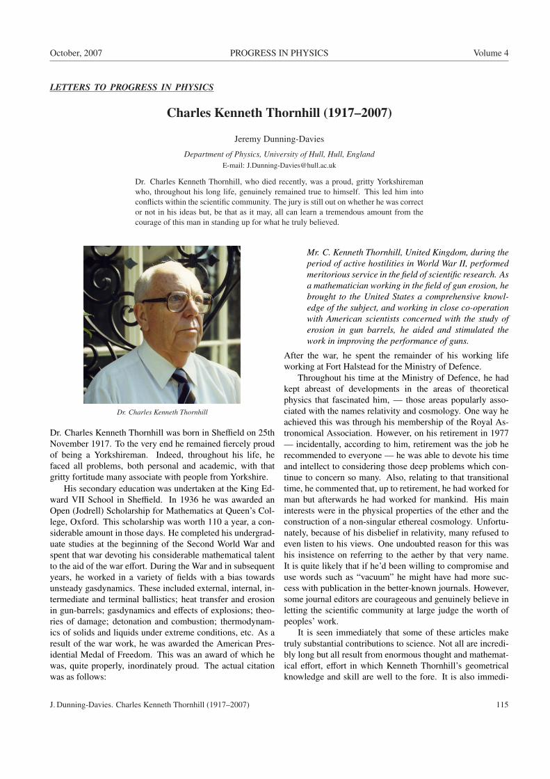
October, 2007 PROGRESS IN PHYSICS Volume 4
LETTERS TO PROGRESS IN PHYSICS
Charles Kenneth Thornhill (1917–2007)
Jeremy Dunning-Davies
Department of Physics, University of Hull, Hull, EnglandE-mail: [email protected]
Dr. Charles Kenneth Thornhill, who died recently, was a proud, gritty Yorkshiremanwho, throughout his long life, genuinely remained true to himself. This led him intoconflicts within the scientific community. The jury is still out on whether he was corrector not in his ideas but, be that as it may, all can learn a tremendous amount from thecourage of this man in standing up for what he truly believed.
Dr. Charles Kenneth Thornhill
Dr. Charles Kenneth Thornhill was born in Sheffield on 25thNovember 1917. To the very end he remained fiercely proudof being a Yorkshireman. Indeed, throughout his life, hefaced all problems, both personal and academic, with thatgritty fortitude many associate with people from Yorkshire.
His secondary education was undertaken at the King Ed-ward VII School in Sheffield. In 1936 he was awarded anOpen (Jodrell) Scholarship for Mathematics at Queen’s Col-lege, Oxford. This scholarship was worth 110 a year, a con-siderable amount in those days. He completed his undergrad-uate studies at the beginning of the Second World War andspent that war devoting his considerable mathematical talentto the aid of the war effort. During the War and in subsequentyears, he worked in a variety of fields with a bias towardsunsteady gasdynamics. These included external, internal, in-termediate and terminal ballistics; heat transfer and erosionin gun-barrels; gasdynamics and effects of explosions; theo-ries of damage; detonation and combustion; thermodynam-ics of solids and liquids under extreme conditions, etc. As aresult of the war work, he was awarded the American Pres-idential Medal of Freedom. This was an award of which hewas, quite properly, inordinately proud. The actual citationwas as follows:
Mr. C. Kenneth Thornhill, United Kingdom, during theperiod of active hostilities in World War II, performedmeritorious service in the field of scientific research. Asa mathematician working in the field of gun erosion, hebrought to the United States a comprehensive knowl-edge of the subject, and working in close co-operationwith American scientists concerned with the study oferosion in gun barrels, he aided and stimulated thework in improving the performance of guns.
After the war, he spent the remainder of his working lifeworking at Fort Halstead for the Ministry of Defence.
Throughout his time at the Ministry of Defence, he hadkept abreast of developments in the areas of theoreticalphysics that fascinated him, — those areas popularly asso-ciated with the names relativity and cosmology. One way heachieved this was through his membership of the Royal As-tronomical Association. However, on his retirement in 1977— incidentally, according to him, retirement was the job herecommended to everyone — he was able to devote his timeand intellect to considering those deep problems which con-tinue to concern so many. Also, relating to that transitionaltime, he commented that, up to retirement, he had worked forman but afterwards he had worked for mankind. His maininterests were in the physical properties of the ether and theconstruction of a non-singular ethereal cosmology. Unfortu-nately, because of his disbelief in relativity, many refused toeven listen to his views. One undoubted reason for this washis insistence on referring to the aether by that very name.It is quite likely that if he’d been willing to compromise anduse words such as “vacuum” he might have had more suc-cess with publication in the better-known journals. However,some journal editors are courageous and genuinely believe inletting the scientific community at large judge the worth ofpeoples’ work.
It is seen immediately that some of these articles maketruly substantial contributions to science. Not all are incredi-bly long but all result from enormous thought and mathemat-ical effort, effort in which Kenneth Thornhill’s geometricalknowledge and skill are well to the fore. It is also immedi-
J. Dunning-Davies. Charles Kenneth Thornhill (1917–2007) 115
Volume 4 PROGRESS IN PHYSICS October, 2007
ately clear that here was a man who was prepared to thinkfor himself and not allow himself to be absolutely bound bywhat appeared in books, whether the books in question beacademic tomes or mere popular offerings.
In his life, Kenneth Thornhill was ostracised by many inthe scientific establishment as some sort of “enfant terrible”.In truth, many of these people really feared his intellect. Thatis not to say that all his thoughts were correct. The jury shouldstill be out on many of his ideas but, to do that, the mem-bers of the jury must have read his offerings and done so withopen scientific minds. Kenneth Thornhill left us all a trulyenormous legacy and that is that he showed us all that it isvitally important to be true to yourself. He never panderedto the establishment rather he stuck with what he genuinelybelieved.
Kenneth Thornhill died peacefully on 30th June 2007 andis survived by four children, eight grandchildren and twogreat grandchildren. To the end he was enormously proud ofall fourteen and to them must be extended our heartfelt sym-pathy. To the scientific community at large must be extendedthe hope that its members will learn the true meaning of scien-tific integrity from this gritty Yorkshireman. As one who wasprivileged to know him, albeit mainly through lengthy, en-joyable telephone conversations, I feel his scientific integrityalone will result in the words:
“Well done, thou good and faithful servant.”
Submitted on August 07, 2007Accepted on August 23, 2007
116 J. Dunning-Davies. Charles Kenneth Thornhill (1917–2007)
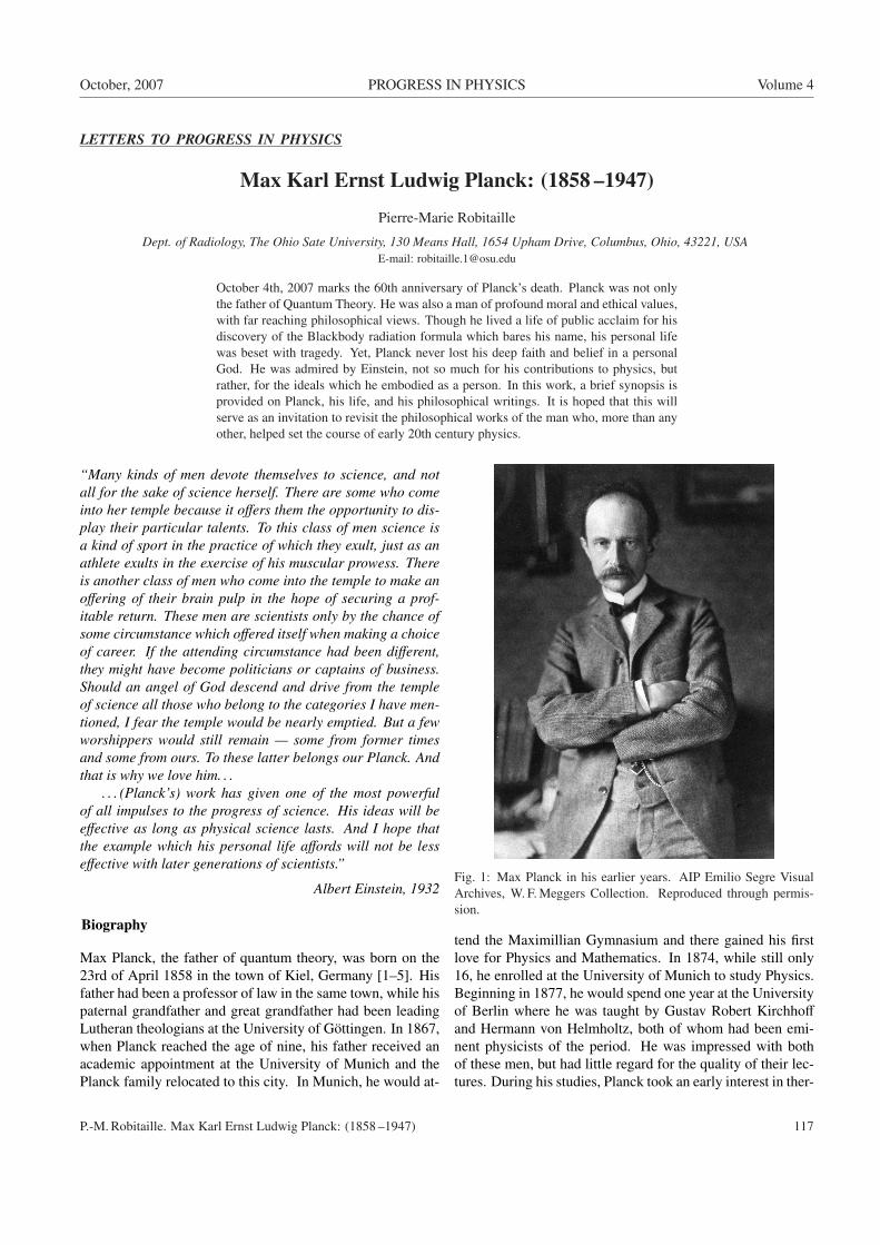
October, 2007 PROGRESS IN PHYSICS Volume 4
LETTERS TO PROGRESS IN PHYSICS
Max Karl Ernst Ludwig Planck: (1858 –1947)
Pierre-Marie Robitaille
Dept. of Radiology, The Ohio Sate University, 130 Means Hall, 1654 Upham Drive, Columbus, Ohio, 43221, USAE-mail: [email protected]
October 4th, 2007 marks the 60th anniversary of Planck’s death. Planck was not onlythe father of Quantum Theory. He was also a man of profound moral and ethical values,with far reaching philosophical views. Though he lived a life of public acclaim for hisdiscovery of the Blackbody radiation formula which bares his name, his personal lifewas beset with tragedy. Yet, Planck never lost his deep faith and belief in a personalGod. He was admired by Einstein, not so much for his contributions to physics, butrather, for the ideals which he embodied as a person. In this work, a brief synopsis isprovided on Planck, his life, and his philosophical writings. It is hoped that this willserve as an invitation to revisit the philosophical works of the man who, more than anyother, helped set the course of early 20th century physics.
“Many kinds of men devote themselves to science, and notall for the sake of science herself. There are some who comeinto her temple because it offers them the opportunity to dis-play their particular talents. To this class of men science isa kind of sport in the practice of which they exult, just as anathlete exults in the exercise of his muscular prowess. Thereis another class of men who come into the temple to make anoffering of their brain pulp in the hope of securing a prof-itable return. These men are scientists only by the chance ofsome circumstance which offered itself when making a choiceof career. If the attending circumstance had been different,they might have become politicians or captains of business.Should an angel of God descend and drive from the templeof science all those who belong to the categories I have men-tioned, I fear the temple would be nearly emptied. But a fewworshippers would still remain — some from former timesand some from ours. To these latter belongs our Planck. Andthat is why we love him. . .
. . . (Planck’s) work has given one of the most powerfulof all impulses to the progress of science. His ideas will beeffective as long as physical science lasts. And I hope thatthe example which his personal life affords will not be lesseffective with later generations of scientists.”
Albert Einstein, 1932
Biography
Max Planck, the father of quantum theory, was born on the23rd of April 1858 in the town of Kiel, Germany [1–5]. Hisfather had been a professor of law in the same town, while hispaternal grandfather and great grandfather had been leadingLutheran theologians at the University of Gottingen. In 1867,when Planck reached the age of nine, his father received anacademic appointment at the University of Munich and thePlanck family relocated to this city. In Munich, he would at-
Fig. 1: Max Planck in his earlier years. AIP Emilio Segre VisualArchives, W. F. Meggers Collection. Reproduced through permis-sion.
tend the Maximillian Gymnasium and there gained his firstlove for Physics and Mathematics. In 1874, while still only16, he enrolled at the University of Munich to study Physics.Beginning in 1877, he would spend one year at the Universityof Berlin where he was taught by Gustav Robert Kirchhoff
and Hermann von Helmholtz, both of whom had been emi-nent physicists of the period. He was impressed with bothof these men, but had little regard for the quality of their lec-tures. During his studies, Planck took an early interest in ther-
P.-M. Robitaille. Max Karl Ernst Ludwig Planck: (1858 –1947) 117
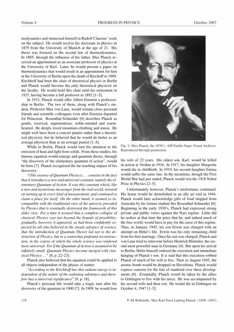
Volume 4 PROGRESS IN PHYSICS October, 2007
modynamics and immersed himself in Rudolf Clausius’ workon the subject. He would receive his doctorate in physics in1879 from the University of Munich at the age of 21. Histhesis was focused on the second law of thermodynamics.In 1885, through the influence of his father, Max Planck re-ceived an appointment as an associate professor of physics atthe University of Kiel. Later, he would present a paper onthermodynamics that would result in an appointment for himat the University of Berlin upon the death of Kirchoff in 1889.Kirchhoff had been the chair of theoretical physics in Berlinand Planck would become the only theoretical physicist onthe faculty. He would hold this chair until his retirement in1927, having become a full professor in 1892 [1–5].
In 1913, Planck would offer Albert Einstein a professor-ship in Berlin. The two of them, along with Planck’s stu-dent, Professor Max von Laue, would remain close personalfriends and scientific colleagues even after Einstein departedfor Princeton. Rosenthal-Schneider [6] describes Planck asgentle, reserved, unpretentious, noble-minded and warm-hearted. He deeply loved mountain-climbing and music. Hemight well have been a concert pianist rather than a theoret-ical physicist, but he believed that he would do better as anaverage physicist than as an average pianist [1, 6].
While in Berlin, Planck would turn his attention to theemission of heat and light from solids. From these studies, hisfamous equation would emerge and quantum theory, through“the discovery of the elementary quantum of action”, wouldbe born [7]. Planck recognized the far reaching impact of hisdiscovery:
“(The essence of Quantum Physics) . . . consists in the factthat it introduces a new and universal constant, namely the el-ementary Quantum of Action. It was this constant which, likea new and mysterious messenger from the real world, insistedon turning up in every kind of measurement, and continued toclaim a place for itself. On the other hand, it seemed so in-compatible with the traditional view of the universe providedby Physics that it eventually destroyed the framework of thisolder view. For a time it seemed that a complete collapse ofclassical Physics was not beyond the bounds of possibility;gradually, however, it appeared, as had been confidently ex-pected by all who believed in the steady advance of science,that the introduction of Quantum Theory led not to the de-struction of Physics, but to a somewhat profound reconstruc-tion, in the course of which the whole science was renderedmore universal. For if the Quantum of Action is assumed to beinfinitely small, Quantum Physics become merged with clas-sical Physics. . . ” [8, p. 22–23].
Planck also believed that his equation could be applied toall objects independent of the phases of matter:
“According to the Kirchhoff law this radiant energy is in-dependent of the nature of the radiating substance and there-fore has a universal significance” [9, p. 18].
Planck’s personal life would take a tragic turn after hisdiscovery of the quantum in 1900 [7]. In 1909, he would lose
Fig. 2: Max Planck, the 1930’s. AIP Emilio Segre Visual Archives.Reproduced through permission.
his wife of 22 years. His oldest son, Karl, would be killedin action at Verdun in 1916. In 1917, his daughter Margeritewould die in childbirth. In 1919, his second daughter Emmawould suffer the same fate. In the meantime, though the FirstWorld War had just ended, Planck would win the 1918 NobelPrize in Physics [2–5].
Unfortunately however, Planck’s misfortunes continued.His home would be demolished in an ally air raid in 1944.Planck would later acknowledge gifts of food shipped fromAustralia by his former student Iles Rosenthal-Schneider [6].Beginning in the early 1930’s, Planck had expressed strongprivate and public views against the Nazi regime. Little didhe realize at that time the price that he, and indeed much ofthe free world, would have to pay for the curse of this regime.Thus, in January 1945, his son Erwin was charged with anattempt on Hitler’s life. Erwin was his only remaining childfrom his first marriage. Once his son was charged, Planck andvon Laue tried to intervene before Heinrich Himmler, the sec-ond most powerful man in Germany [4]. But upon his arrivalto Berlin, Hitler himself ordered the execution and immediatehanging of Planck’s son. It is said that this execution robbedPlanck of much of his will to live. Then in August 1945, theatomic bomb would be dropped on Hiroshima. Planck wouldexpress concern for the fate of mankind over these develop-ments [6]. Eventually, Planck would be taken by the alliesto Gottingen to live with his niece. He was accompanied byhis second wife and their son. He would die in Gottingen onOctober 4, 1947 [1–5].
118 P.-M. Robitaille. Max Karl Ernst Ludwig Planck: (1858 –1947)
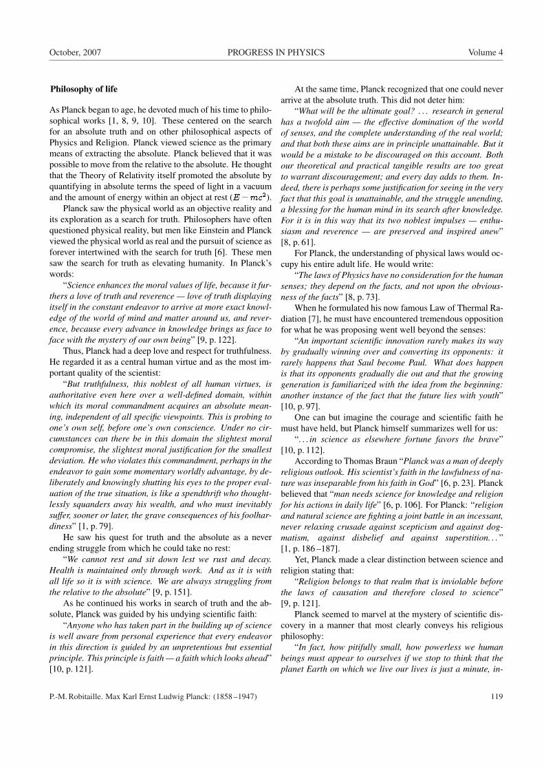
October, 2007 PROGRESS IN PHYSICS Volume 4
Philosophy of life
As Planck began to age, he devoted much of his time to philo-sophical works [1, 8, 9, 10]. These centered on the searchfor an absolute truth and on other philosophical aspects ofPhysics and Religion. Planck viewed science as the primarymeans of extracting the absolute. Planck believed that it waspossible to move from the relative to the absolute. He thoughtthat the Theory of Relativity itself promoted the absolute byquantifying in absolute terms the speed of light in a vacuumand the amount of energy within an object at rest (E=mc2).
Planck saw the physical world as an objective reality andits exploration as a search for truth. Philosophers have oftenquestioned physical reality, but men like Einstein and Planckviewed the physical world as real and the pursuit of science asforever intertwined with the search for truth [6]. These mensaw the search for truth as elevating humanity. In Planck’swords:
“Science enhances the moral values of life, because it fur-thers a love of truth and reverence — love of truth displayingitself in the constant endeavor to arrive at more exact knowl-edge of the world of mind and matter around us, and rever-ence, because every advance in knowledge brings us face toface with the mystery of our own being” [9, p. 122].
Thus, Planck had a deep love and respect for truthfulness.He regarded it as a central human virtue and as the most im-portant quality of the scientist:
“But truthfulness, this noblest of all human virtues, isauthoritative even here over a well-defined domain, withinwhich its moral commandment acquires an absolute mean-ing, independent of all specific viewpoints. This is probing toone’s own self, before one’s own conscience. Under no cir-cumstances can there be in this domain the slightest moralcompromise, the slightest moral justification for the smallestdeviation. He who violates this commandment, perhaps in theendeavor to gain some momentary worldly advantage, by de-liberately and knowingly shutting his eyes to the proper eval-uation of the true situation, is like a spendthrift who thought-lessly squanders away his wealth, and who must inevitablysuffer, sooner or later, the grave consequences of his foolhar-diness” [1, p. 79].
He saw his quest for truth and the absolute as a neverending struggle from which he could take no rest:
“We cannot rest and sit down lest we rust and decay.Health is maintained only through work. And as it is withall life so it is with science. We are always struggling fromthe relative to the absolute” [9, p. 151].
As he continued his works in search of truth and the ab-solute, Planck was guided by his undying scientific faith:
“Anyone who has taken part in the building up of scienceis well aware from personal experience that every endeavorin this direction is guided by an unpretentious but essentialprinciple. This principle is faith — a faith which looks ahead”[10, p. 121].
At the same time, Planck recognized that one could neverarrive at the absolute truth. This did not deter him:
“What will be the ultimate goal? . . . research in generalhas a twofold aim — the effective domination of the worldof senses, and the complete understanding of the real world;and that both these aims are in principle unattainable. But itwould be a mistake to be discouraged on this account. Bothour theoretical and practical tangible results are too greatto warrant discouragement; and every day adds to them. In-deed, there is perhaps some justification for seeing in the veryfact that this goal is unattainable, and the struggle unending,a blessing for the human mind in its search after knowledge.For it is in this way that its two noblest impulses — enthu-siasm and reverence — are preserved and inspired anew”[8, p. 61].
For Planck, the understanding of physical laws would oc-cupy his entire adult life. He would write:
“The laws of Physics have no consideration for the humansenses; they depend on the facts, and not upon the obvious-ness of the facts” [8, p. 73].
When he formulated his now famous Law of Thermal Ra-diation [7], he must have encountered tremendous oppositionfor what he was proposing went well beyond the senses:
“An important scientific innovation rarely makes its wayby gradually winning over and converting its opponents: itrarely happens that Saul become Paul. What does happenis that its opponents gradually die out and that the growinggeneration is familiarized with the idea from the beginning:another instance of the fact that the future lies with youth”[10, p. 97].
One can but imagine the courage and scientific faith hemust have held, but Planck himself summarizes well for us:
“. . . in science as elsewhere fortune favors the brave”[10, p. 112].
According to Thomas Braun “Planck was a man of deeplyreligious outlook. His scientist’s faith in the lawfulness of na-ture was inseparable from his faith in God” [6, p. 23]. Planckbelieved that “man needs science for knowledge and religionfor his actions in daily life” [6, p. 106]. For Planck: “religionand natural science are fighting a joint battle in an incessant,never relaxing crusade against scepticism and against dog-matism, against disbelief and against superstition. . . ”[1, p. 186 –187].
Yet, Planck made a clear distinction between science andreligion stating that:
“Religion belongs to that realm that is inviolable beforethe laws of causation and therefore closed to science”[9, p. 121].
Planck seemed to marvel at the mystery of scientific dis-covery in a manner that most clearly conveys his religiousphilosophy:
“In fact, how pitifully small, how powerless we humanbeings must appear to ourselves if we stop to think that theplanet Earth on which we live our lives is just a minute, in-
P.-M. Robitaille. Max Karl Ernst Ludwig Planck: (1858 –1947) 119
Volume 4 PROGRESS IN PHYSICS October, 2007
finitesimal mote of dust; on the other hand how peculiar itmust seem that we, tiny creatures on a tiny planet, are nev-ertheless capable of knowing though not the essence at leastthe existence and the dimensions of the basic building blocksof the entire great Cosmos!” [1, p. 174].
Perhaps there is no more suitable way of closing a workon Max Planck than to recall the memorial address deliveredby Professor Max von Laue at the Albani Church in Gottin-gen on October 7, 1947 [1, p. 7–10]. Max von Laue was acolleague of Max Planck at the University of Berlin. In 1914,he had received the Nobel Prize in Physics for his study of thediffraction of X-rays by crystals.
My Fellow Mourners:We stand at the bier of a man who lived to be almost four-
score-and-ten. Ninety years are a long life, and these par-ticular ninety years were extraordinarily rich in experiences.Max Planck would remember, even in his old age, the sightof the Prussian and Austrian troops marching into his na-tive town of Kiel. The birth and meteoric ascent of the Ger-man Empire occurred during his lifetime, and so did its totaleclipse and ghastly disaster. These events had a most pro-found effect on Planck in his person, too. His eldest son, Karl,died in action at Verdun in 1916. In the Second World War, hishouse went up in flames during an air raid. His library, col-lected throughout a whole long lifetime, disappeared, no oneknows where, and the most terrible blow of all fell when hissecond son, Erwin, lost his life in the rule of terror in January,1945. While on a lecture tour, Max Planck, himself, was aneye-witness of the destruction of Kassel, and was buried in anair raid shelter for several hours. In the middle of May, 1945,the Americans sent a car to his estate of Rogatz on the Elbe,then a theatre of war, to take him to Gottingen. Now we aretaking him to his final resting-place.
In the field of science, too, Planck’s lifetime was an epochof deep-reaching changes. The physical science of our daysshows an aspect totally different from that of 1875, whenPlanck began to devote himself to it — and Max Planck isentitled to the lion’s share in the credit for these changes.And what a wonderous story his life was! Just think — boyof seventeen, just graduated from high school, he decided totake up a science which even its most authoritative repre-sentative who he could consult, described as one of mightymeager prospects. As a student, he chose a certain branchof science, for which even its neighbor sciences had but lit-tle regard — and even within this particular branch a highlyspecialized field, in which literally nobody at all had any in-terest whatever. His first scientific papers were not read byHelmholtz, Kirchhoff and Clausius, the very men who wouldhave found it easiest to appreciate them. Yet, he continued onhis way, obeying an inner call, until he came face to face witha problem which many others had tried and failed to solve, aproblem for which the very path taken by him turned out tohave been the best preparation. Thus, he was able to recog-nize and formulate, from measurements of radiations, the law
which today bears and immortalizes his name for all times.He announced it before the Berlin Physical Society on Octo-ber 19, 1900. To be sure, the theoretical substantiation of itmade it necessary for him to reconsider his views and to fallback on methods of the atom theory, which he had been wontto regard with certain doubts, And beyond that, he had to ven-ture a hypothesis, the audacity of which was not clear at first,to its full extent, to anybody, not even him. But on December14, 1900, again before the German Physical Society, he wasable to present the theoretic deduction of the law of radiation.This was the birthday of quantum theory. This achievementwill perpetuate his name forever.
Max von Laue, 1947
First Published Online on June 23, 2001on http://www.thermalphysics.org
Revised March 14, 2002Submitted on September 11, 2007Accepted on September 17, 2007
Published online on October 04, 2007
References
1. Planck M. Scientific autobiography. Philosophical Library,New York, 1949.
2. Max Planck in: The Nobel Foundation — Online, http://www.nobel.se/physics/laureates/1918/index.html
3. Cannon B.D. Max Planck 1918. In: “The Nobel Prize Winners:Physics” (Frank N. Magill, Ed.), Salem Press, Pasadena, Cali-fornia, 1989.
4. Max Planck in: Encyclopedia Britanica, see Encyclope-dia Britanica Online, http://www.britannica.com/eb/article–9108525/Max–Planck
5. Max Planck in: Index of Biographies, School of Mathematicsand Statistics, University of St. Andrews, Scottland, U.K.http://www.groups.dcs.st-and.ac.uk/�history/Mathematicians/Planck.html
6. Rosenthal-Schneider I. Reality and scientific thruth: discus-sions with Einstein, von Laue and Planck. Wayne State Uni-versity Press, Detroit, 1980.
7. Planck M. Ueber das Gesetz der Energieverteilung in Normal-spectrum. Ann. Phys., 1901, v. 4, 553–563.
8. Planck M. The Universe in the light of modern physics. W.W.Norton & Company, Inc., New York, 1931.
9. Planck M. The new science. Meridian Books, Inc., New York,1959.
10. Planck M. Philosophy of physics. W.W. Norton & CompanyInc., New York, 1936.
120 P.-M. Robitaille. Max Karl Ernst Ludwig Planck: (1858 –1947)
Progress in Physics is a quarterly issue scientific journal, registered withthe Library of Congress (DC).
This is a journal for scientific publications on advanced studies in theor-etical and experimental physics, including related themes from mathem-atics.
Electronic version of this journal:http://www.ptep-online.com
Editor in Chief
Dmitri Rabounski [email protected]
Associate Editors
Florentin SmarandacheLarissa BorissovaStephen J. Crothers
Progress in Physics is peer reviewed and included in the abstractingand indexing coverage of: Mathematical Reviews and MathSciNet ofAMS (USA), DOAJ of Lund University (Sweden), Zentralblatt MATH(Germany), Referativnyi Zhurnal VINITI (Russia), etc.
Department of Mathematics and Science, University of New Mexico,200 College Road, Gallup, NM 87301, USA
Printed in the United States of America
Issue 2007, Volume 4US $ 20.00