
Project Lambda: Functional Programming Constructs & Simpler Concurrency In Java SE 8

Programming Languages and Lambda Calculi(Utah CS7520 Version)
Matthias Felleisen Matthew Flatt
Draft: March 8, 2006
Copyright c©1989, 2003 Felleisen, Flatt

2

Contents
I Models of Languages 7
Chapter 1: Computing with Text 91.1 Defining Sets . . . . . . . . . . . . . . . . . . . . . . . . . . . . . . . . . . . . . . 91.2 Relations . . . . . . . . . . . . . . . . . . . . . . . . . . . . . . . . . . . . . . . . 101.3 Relations as Evaluation . . . . . . . . . . . . . . . . . . . . . . . . . . . . . . . . 111.4 Directed Evaluation . . . . . . . . . . . . . . . . . . . . . . . . . . . . . . . . . . 111.5 Evaluation in Context . . . . . . . . . . . . . . . . . . . . . . . . . . . . . . . . . 121.6 Evaluation Function . . . . . . . . . . . . . . . . . . . . . . . . . . . . . . . . . . 131.7 Notation Summary . . . . . . . . . . . . . . . . . . . . . . . . . . . . . . . . . . . 13
Chapter 2: Structural Induction 152.1 Detecting the Need for Structural Induction . . . . . . . . . . . . . . . . . . . . . 152.2 Definitions with Ellipses . . . . . . . . . . . . . . . . . . . . . . . . . . . . . . . . 172.3 Induction on Proof Trees . . . . . . . . . . . . . . . . . . . . . . . . . . . . . . . . 172.4 Multiple Structures . . . . . . . . . . . . . . . . . . . . . . . . . . . . . . . . . . . 182.5 More Definitions and More Proofs . . . . . . . . . . . . . . . . . . . . . . . . . . 19
Chapter 3: Consistency of Evaluation 21
Chapter 4: The λ-Calculus 254.1 Functions in the λ-Calculus . . . . . . . . . . . . . . . . . . . . . . . . . . . . . . 254.2 λ-Calculus Grammar and Reductions . . . . . . . . . . . . . . . . . . . . . . . . . 264.3 Encoding Booleans . . . . . . . . . . . . . . . . . . . . . . . . . . . . . . . . . . . 284.4 Encoding Pairs . . . . . . . . . . . . . . . . . . . . . . . . . . . . . . . . . . . . . 294.5 Encoding Numbers . . . . . . . . . . . . . . . . . . . . . . . . . . . . . . . . . . . 304.6 Recursion . . . . . . . . . . . . . . . . . . . . . . . . . . . . . . . . . . . . . . . . 31
4.6.1 Recursion via Self-Application . . . . . . . . . . . . . . . . . . . . . . . . 324.6.2 Lifting Out Self-Application . . . . . . . . . . . . . . . . . . . . . . . . . . 334.6.3 Fixed Points and the Y Combinator . . . . . . . . . . . . . . . . . . . . . 34
4.7 Facts About the λ-Calculus . . . . . . . . . . . . . . . . . . . . . . . . . . . . . . 354.8 History . . . . . . . . . . . . . . . . . . . . . . . . . . . . . . . . . . . . . . . . . 37
II Models of Realistic Languages 39
Chapter 5: ISWIM 415.1 ISWIM Expressions . . . . . . . . . . . . . . . . . . . . . . . . . . . . . . . . . . 415.2 ISWIM Reductions . . . . . . . . . . . . . . . . . . . . . . . . . . . . . . . . . . . 425.3 The Yv Combinator . . . . . . . . . . . . . . . . . . . . . . . . . . . . . . . . . . 435.4 Evaluation . . . . . . . . . . . . . . . . . . . . . . . . . . . . . . . . . . . . . . . . 455.5 Consistency . . . . . . . . . . . . . . . . . . . . . . . . . . . . . . . . . . . . . . . 45
3

4
5.6 Observational Equivalence . . . . . . . . . . . . . . . . . . . . . . . . . . . . . . . 495.7 History . . . . . . . . . . . . . . . . . . . . . . . . . . . . . . . . . . . . . . . . . 51
Chapter 6: Standard Reduction 536.1 Standard Reductions . . . . . . . . . . . . . . . . . . . . . . . . . . . . . . . . . . 536.2 Proving the Standard Reduction Theorem . . . . . . . . . . . . . . . . . . . . . . 566.3 Observational Equivalence . . . . . . . . . . . . . . . . . . . . . . . . . . . . . . . 636.4 Uniform Evaluation . . . . . . . . . . . . . . . . . . . . . . . . . . . . . . . . . . 66
Chapter 7: Machines 697.1 CC Machine . . . . . . . . . . . . . . . . . . . . . . . . . . . . . . . . . . . . . . . 697.2 SCC Machine . . . . . . . . . . . . . . . . . . . . . . . . . . . . . . . . . . . . . . 727.3 CK Machine . . . . . . . . . . . . . . . . . . . . . . . . . . . . . . . . . . . . . . . 757.4 CEK Machine . . . . . . . . . . . . . . . . . . . . . . . . . . . . . . . . . . . . . . 777.5 Machine Summary . . . . . . . . . . . . . . . . . . . . . . . . . . . . . . . . . . . 81
Chapter 8: SECD, Tail Calls, and Safe for Space 838.1 SECD machine . . . . . . . . . . . . . . . . . . . . . . . . . . . . . . . . . . . . . 838.2 Context Space . . . . . . . . . . . . . . . . . . . . . . . . . . . . . . . . . . . . . 848.3 Environment Space . . . . . . . . . . . . . . . . . . . . . . . . . . . . . . . . . . . 868.4 History . . . . . . . . . . . . . . . . . . . . . . . . . . . . . . . . . . . . . . . . . 87
Chapter 9: Continuations 899.1 Saving Contexts . . . . . . . . . . . . . . . . . . . . . . . . . . . . . . . . . . . . 899.2 Revised Texual Machine . . . . . . . . . . . . . . . . . . . . . . . . . . . . . . . . 909.3 Revised CEK Machine . . . . . . . . . . . . . . . . . . . . . . . . . . . . . . . . . 91
Chapter 10: Errors and Exceptions 9310.1 Errors . . . . . . . . . . . . . . . . . . . . . . . . . . . . . . . . . . . . . . . . . . 93
10.1.1 Calculating with Error ISWIM . . . . . . . . . . . . . . . . . . . . . . . . 9310.1.2 Consistency for Error ISWIM . . . . . . . . . . . . . . . . . . . . . . . . . 9510.1.3 Standard Reduction for Error ISWIM . . . . . . . . . . . . . . . . . . . . 9810.1.4 Relating ISWIM and Error ISWIM . . . . . . . . . . . . . . . . . . . . . . 99
10.2 Exceptions and Handlers . . . . . . . . . . . . . . . . . . . . . . . . . . . . . . . . 10210.2.1 Calculating with Handler ISWIM . . . . . . . . . . . . . . . . . . . . . . . 10310.2.2 Consistency for Handler ISWIM . . . . . . . . . . . . . . . . . . . . . . . 10410.2.3 Standard Reduction for Handler ISWIM . . . . . . . . . . . . . . . . . . . 10510.2.4 Observational Equivalence of Handler ISWIM . . . . . . . . . . . . . . . . 106
10.3 Machines for Exceptions . . . . . . . . . . . . . . . . . . . . . . . . . . . . . . . . 10710.3.1 The Handler-Extended CC Machine . . . . . . . . . . . . . . . . . . . . . 10710.3.2 The CCH Machine . . . . . . . . . . . . . . . . . . . . . . . . . . . . . . . 108
Chapter 11: Imperative Assignment 11111.1 Evaluation with State . . . . . . . . . . . . . . . . . . . . . . . . . . . . . . . . . 11111.2 Garbage Collection . . . . . . . . . . . . . . . . . . . . . . . . . . . . . . . . . . . 11411.3 CEKS Machine . . . . . . . . . . . . . . . . . . . . . . . . . . . . . . . . . . . . . 11611.4 Implementing Garbage Collection . . . . . . . . . . . . . . . . . . . . . . . . . . . 11711.5 History . . . . . . . . . . . . . . . . . . . . . . . . . . . . . . . . . . . . . . . . . 118

5
III Models of Typed Languages 119
Chapter 12: Types 12112.1 Numbers and Booleans . . . . . . . . . . . . . . . . . . . . . . . . . . . . . . . . . 12212.2 Soundness . . . . . . . . . . . . . . . . . . . . . . . . . . . . . . . . . . . . . . . . 124
Chapter 13: Simply Typed ISWIM 12713.1 Function Types . . . . . . . . . . . . . . . . . . . . . . . . . . . . . . . . . . . . . 12713.2 Type Rules for Simply Typed ISWIM . . . . . . . . . . . . . . . . . . . . . . . . 12813.3 Soundness . . . . . . . . . . . . . . . . . . . . . . . . . . . . . . . . . . . . . . . . 13013.4 Normalization . . . . . . . . . . . . . . . . . . . . . . . . . . . . . . . . . . . . . . 131
Chapter 14: Variations on Simply Typed ISWIM 13514.1 Conditionals . . . . . . . . . . . . . . . . . . . . . . . . . . . . . . . . . . . . . . . 13514.2 Pairs . . . . . . . . . . . . . . . . . . . . . . . . . . . . . . . . . . . . . . . . . . . 13614.3 Variants . . . . . . . . . . . . . . . . . . . . . . . . . . . . . . . . . . . . . . . . . 13714.4 Recursion . . . . . . . . . . . . . . . . . . . . . . . . . . . . . . . . . . . . . . . . 138
Chapter 15: Polymorphism 14115.1 Polymorphic ISWIM . . . . . . . . . . . . . . . . . . . . . . . . . . . . . . . . . . 141
Chapter 16: Type Inference 14516.1 Type-Inferred ISWIM . . . . . . . . . . . . . . . . . . . . . . . . . . . . . . . . . 145
16.1.1 Constraint Generation . . . . . . . . . . . . . . . . . . . . . . . . . . . . . 14616.1.2 Unification . . . . . . . . . . . . . . . . . . . . . . . . . . . . . . . . . . . 147
16.2 Inferring Polymorphism . . . . . . . . . . . . . . . . . . . . . . . . . . . . . . . . 149
Chapter 17: Recursive Types 15117.1 Fixed-points of Type Abstractions . . . . . . . . . . . . . . . . . . . . . . . . . . 15117.2 Equality Between Recursive Types . . . . . . . . . . . . . . . . . . . . . . . . . . 15217.3 Isomorphisms Between Recursive Types . . . . . . . . . . . . . . . . . . . . . . . 15317.4 Using Iso-Recursive Types . . . . . . . . . . . . . . . . . . . . . . . . . . . . . . . 154
Chapter 18: Data Abstraction and Existential Types 15718.1 Data Abstraction in Clients . . . . . . . . . . . . . . . . . . . . . . . . . . . . . . 15718.2 Libraries that Enforce Abstraction . . . . . . . . . . . . . . . . . . . . . . . . . . 15818.3 Existential ISWIM . . . . . . . . . . . . . . . . . . . . . . . . . . . . . . . . . . . 15918.4 Modules and Existential Types . . . . . . . . . . . . . . . . . . . . . . . . . . . . 161
Chapter 19: Subtyping 16319.1 Records and Subtypes . . . . . . . . . . . . . . . . . . . . . . . . . . . . . . . . . 16319.2 Subtypes and Functions . . . . . . . . . . . . . . . . . . . . . . . . . . . . . . . . 16519.3 Subtypes and Fields . . . . . . . . . . . . . . . . . . . . . . . . . . . . . . . . . . 16619.4 From Records to Objects . . . . . . . . . . . . . . . . . . . . . . . . . . . . . . . 166
Chapter 20: Objects and Classes 16920.1 MiniJava Syntax . . . . . . . . . . . . . . . . . . . . . . . . . . . . . . . . . . . . 16920.2 MiniJava Evaluation . . . . . . . . . . . . . . . . . . . . . . . . . . . . . . . . . . 17220.3 MiniJava Type Checking . . . . . . . . . . . . . . . . . . . . . . . . . . . . . . . . 17320.4 MiniJava Soundness . . . . . . . . . . . . . . . . . . . . . . . . . . . . . . . . . . 17520.5 MiniJava Summary . . . . . . . . . . . . . . . . . . . . . . . . . . . . . . . . . . . 181

6

Part I
Models of Languages
7


9
Chapter 1: Computing with Text
In this book, we study how a programming language can be defined in a way that is easilyunderstood by people, and also amenable to formal analysis—where the formal analysis shouldbe easily understood by people, too.
One way of defining a language is to write prose paragraphs that explain the kinds ofexpressions that are allowed in the language and how they are evaluated. This technique hasan advantage that a reader can quickly absorb general ideas about the language, but detailsabout the language are typically difficult to extract from prose. Worse, prose does not lenditself to formal analysis.
Another way of defining a language is to implement an interpreter for it in some meta-language. Assuming that a reader is familiar with the meta-language, this technique has theadvantage of clearly and completely specifying the details of the language. Assuming that themeta-language has a formal specification, then the interpreter has a formal meaning in thatlanguage, and it can be analyzed.
The meta-language used to define another language need not execute efficiently, since itsprimary purpose is to explain the other language to humans. The meta-language’s primitivedata constructs need not be defined in terms of bits and bytes. Indeed, for the meta-languagewe can directly use logic and set theory over a universe of program text. In the same waythat computation on physical machines can be described, ultimately, in terms of shuffling bitsamong memory locations, computation in the abstract can be described in terms of relationson text.
1.1 Defining Sets
When we write a BNF grammar, such as
B = t| f| (B •B)
then we actually define a set B of textual strings. The above definition can be expanded to thefollowing constraints on B:
t ∈ Bf ∈ B
a ∈ B and b ∈ B ⇒ (a • b) ∈ B
Technically, the set B that we mean is the smallest set that obeys the above constraints.Notation: we’ll sometimes use “B” to mean “the set B”, but sometimes “B” will mean “an
arbitrary element of B”. The meaning is always clear from the context. Sometimes, we use asubscript or a prime on the name of the set to indicate an arbitrary element of the set, such as“B1” or “B′”. Thus, the above constraints might be written as
t ∈ B [a]
f ∈ B [b]
(B1 •B2) ∈ B [c]
Whether expressed in BNF shorthand or expanded as a set of constraints, set B is definedrecursively. Enumerating all of the elements of B in finite space is clearly impossible in thiscase:
B = t, f, (t • t), (t • f), . . .

10 Chapter 1: Computing with Text
Given a particular bit of text that belongs to B, however, we can demonstrate that it is in B byshowing how the constraints that define B require the text to be in B. For example, (t• (f•t))is in B:
1. t ∈ B by [a]
2. f ∈ B by [b]
3. t ∈ B by [a]
4. (f • t) ∈ B by 2, 3, and [c]
5. (t • (f • t)) ∈ B by 1, 4, and [c]
We’ll typically write such arguments in proof-tree form:
t ∈ B [a]
f ∈ B [b] t ∈ B [a]
(f • t) ∈ B [c]
(t • (f • t)) ∈ B [c]
Also, we’ll tend to omit the names of deployed rules from the tree, since they’re usually obvious:
t ∈ Bf ∈ B t ∈ B
(f • t) ∈ B(t • (f • t)) ∈ B
Exercise 1.1. Which of the following are in B? For each member of B, provide a proof treeshowing that it must be in B.
1. t
2. •
3. ((f • t) • (f • f))
4. ((f) • (t))
1.2 Relations
A relation is a set whose elements consist of ordered pairs.1 For example, we can define the≡ relation to match each element of B with itself:
a ∈ B ⇒ 〈a, a〉 ∈≡
For binary relations such as ≡, instead of 〈a, a〉 ∈≡, we usually write a ≡ a:
a ∈ B ⇒ a ≡ a
or even simplyB1 ≡ B1
as long as it is understood as a definition of ≡. As it turns out, the relation ≡ is reflexive,symmetric, and transitive:
a relation R is reflexive iff aR a (for any a)a relation R is symmetric iff aR b⇒ bR aa relation R is transitive iff aR b and bR c⇒ aR c
1An ordered pair 〈x, y〉 can be represented as a set of sets x, x, y.

1.3 Relations as Evaluation 11
If a relation is reflexive, symmetric, and transitive, then it is an equivalence.The following defines a relation r that is neither reflexive, symmetric, nor transitive:
(f •B1) r B1 [a]
(t •B1) r t [b]
Using r , we could define a new relation r by adding the constraint that r is reflexive:
(f •B1) r B1 [a]
(t •B1) r t [b]
B1 r B1 [c]
The relation r is the reflexive closure of the r relation. We could define yet another relationby adding symmetric and transitive constraints:
(f •B1) ≈r B1 [a]
(t •B1) ≈r t [b]
B1 ≈r B1 [c]
B1 ≈r B2 ⇒ B2 ≈r B1 [d]
B1 ≈r B2 and B2 ≈r B3 ⇒ B1 ≈r B3 [e]
The≈r relation is the symmetric–transitive closure ofr, and it is the reflexive–symmetric–transitive closure or equivalence closure of r .
1.3 Relations as Evaluation
The running example of B and r should give you an idea of how a programming language canbe defined through text and relations on text—or, more specifically, through a set (B) and arelation on the set ( r ).
In fact, you might begin to suspect that B is a grammar for boolean expressions with • as“or”, and ≈r equates pairs of expressions that have the same boolean value.
Indeed, using the constraints above, we can show that (f•t) ≈r (t•t), just as false∨ true =true ∨ true:
(f • t) ≈r t [a]
(t • t) ≈r t [b]
t ≈r (t • t) [d]
(f • t) ≈r (t • t) [e]
However, it does not follow directly that • is exactly like a boolean “or”. Instead, we wouldhave to prove general claims about •, such as the fact that (B1 • t) ≈r t for any expression B1.(It turns out that we would not be able to prove the claim, as we’ll soon see.)
In other words, there is generally a gap between an interpreter-defined language (even if theinterpreter is defined with mathematics) and properties of the language that we might like toguarantee. For various purposes, the properties of a language are as important as the valuesit computes. For example, if • really acted like “or”, then a compiler might safely optimize(B1 • t) as t. Similarly, if syntactic rules for a language gurantee that a number can never beadded to any value other than another number, then the implementation of the language neednot check the arguments of an addition expression to ensure that they are numbers.
Before we can start to address such gaps, however, we must eliminate a meta-gap betweenthe way that we define languages and the way that normal evaluation proceeds.
1.4 Directed Evaluation
The “evaluation” rule ≈r is not especially evaluation-like. It allows us to prove that certainexpressions are equivalent, but it doesn’t tell us exactly how to get from an arbitrary B toeither t or f.

12 Chapter 1: Computing with Text
The simpler relation r was actually more useful in this sense. Both cases in the definitionof r map an expression to a smaller expression. Also, for any expression B, either B is t or f,or r relates B to at most one other expression. As a result, we can think of r as a single-stepreduction, corresponding to the way that an interpreter might take a single evaluation step inworking towards a final value.
We can define ;;r as the reflexive–transitive closure of r , and we end up with a multi-step reduction relation. The multi-step relation ;;r will map each expression to many otherexpressions. As it turns out, though, ;;r maps each expression to at most one of t or f.
It’s sufficient to define ;;r as “the reflexive–transitive closure of r ”. An alternateformulation would be to expand out the constraints, as in the previous section. Athird way would be to partially expand the constraints, but use r in the definitionof ;;r :
B1 ;;r B1
B1 rB2 ⇒ B1 ;;r B2
B1 ;;r B2 and B2 ;;r B3 ⇒ B1 ;;r B3
The relations r and ;;r are intentionally asymmetric, corresponding to the fact that evaluationshould proceed in a specific direction towards a value. For example, given the expression(f • (f • (t • f))), we can show a reduction to t:
(f • (f • (t • f))) r (f • (t • f))r (t • f)r t
Each blank line in the left column is implicitly filled by the expression in the right column fromthe previous line. Each line is then a step in an argument that (f • (f • (t • f)));;r t.
Exercise 1.2. Show that (f • (f • (f • f)));;r f by showing its reduction with the r one-steprelation.
1.5 Evaluation in Context
How does the expression ((f • t) • f) reduce? According to r or ;;r , it does not reduce at all!Intuitively, ((f•t)•f) should reduce to (t•f), by simplifying the first subexpression according
to (f • t) r f. But there is no constraint in the definition of r that matches ((f • t) • f) as thesource expression. We can only reduce expressions of the form (f • B) and (t • B). In otherwords, the expression on the right-hand side of the outermost • is arbitrary, but the expressionon the left-hand side must be f or t.
We can extend the r relation with →r to support the reduction of subexpressions:
B1 rB2 ⇒ B1 →r B2 [a]
B1 →r B′1 ⇒ (B1 •B2)→r (B′
1 •B2) [b]
B2 →r B′2 ⇒ (B1 •B2)→r (B1 •B′
2) [c]
The →r relation is the compatible closure of the r relation. Like r , →r is a single-stepreduction relation, but →r allows the reduction of any subexpression within the whole expres-sion. The subexpression reduced with r is called the redex, and the text surrounding a redexis its context.
In particular, the →r relation includes ((f • t) • f) →r (t • f). We can demonstrate thisinclusion with the following proof tree:
(f • t) r t(f • t)→r t [a]
((f • t) • f)→r (t • f) [b]

1.6 Evaluation Function 13
Continuing with →r, we can reduce ((f • t) • f) to t:
((f • t) • f) →r (t • f)→r t
Finally, if we define →→r to be the reflexive–transitive closure of →r, then we get ((f • t) •f)→→r t. Thus, →→r is the natural reduction relation generated by r .
In general, the mere reflexive closure r, equivalence closure ≈r, or reflexive-transitiveclosure ;;r of a relation r will be uninteresting. Instead, we’ll most often be interested inthe compatible closure →r and its reflexive–transitive closure →→r , because they correspondto typical notions of evaluation. In addition, the equivalence closure =r of →r is interestingbecause it relates expressions that produce the same result.
Exercise 1.3. Explain why (f • ((t • f) • f)) 6;;r t.
Exercise 1.4. Show that (f • ((t • f) • f))→→r t by demonstrating a reduction with →r.
1.6 Evaluation Function
The →→r brings us close to a useful notion of evaluation, but we are not there yet. While((f • t) • f)→→r t, it’s also the case that ((f • t) • f)→→r (t • f) and ((f • t) • f)→→r ((f • t) • f).
For evaluation, we’re interested in whether B evaluates to f or to t; any other mapping by→→r or =r is irrelevant. To capture this notion of evaluation, we define the evalr relation asfollows:
evalr(B) =
f if B =r ft if B =r t
Here, we’re using yet another notation to define a relation. This particular notation is suggestiveof a function, i.e., a relation that maps each element to at most one element. We use thefunction notation because evalr must be a function if it’s going to make sense as an evaluator.
Exercise 1.5. Among the relations r , r, ≈r, ;;r , →r, →→r , =r, and evalr, which arefunctions? For each non-function relation, find an expression and two expressions that it relatesto.
1.7 Notation Summary
name definition intuitionthe base relation on members a single “reduction” stepof an expression grammar with no context
→ the compatible closure of with a single step within a contextrespect to the expression grammar
→→ the reflexive–transitive closure multiple evaluation stepsof → (zero or more)
= the symmetric–transitive closure equates expressions thatof →→ produce the same result
eval = restricted to a range complete evaluationof results

14 Chapter 1: Computing with Text

15
Chapter 2: Structural Induction
The relation r defined in the previous lecture is a function, but how could we prove it? Here’sa semi-formal argument: The relation r is defined by a pair of constraints. The first constraintapplies to a • expression that starts with f, and the result is determined uniquely by the right-hand part of the expression. The second constraint applies to a • expression that starts witht, and the result is determined uniquely as t. Since an expression can start with either f or t,then only one constraint will apply, and the result is unique.
The above argument is fairly convincing because it relies on a directly observable propertyof the expression: whether it is a • expression that starts with f or t. Other claims aboutrelations over B may not be so simple to prove. For example, it is not immediately obviousthat evalr is a function. The fundamental reason is that B is recursively defined; there is noway to enumerate all of the interesting cases directly. To prove more general claims, we mustuse induction.
Mathematical induction arguments are based on the natural numbers. A claim is provedfor 0, then for n + 1 assuming the claim for n, and then the claim follows for all n. For mostof the proofs we will consider, no natural number n is readily provided for elements of the set(such as B), but one could be derived for an expression based on the number of steps in anargument that the expression belongs to the set (as in §1.1).
Instead of finding appropriate numbers for set elements to enable mathematical induction,however, we will use structural induction, which operates directly on the grammar definingset elements. The underlying principle is the same.
2.1 Detecting the Need for Structural Induction
Structural induction applies when proving a claim about a recursively-defined set. The setis well-founded, of course, only if there are atomic elements in the definition; those elementsconstitute the base cases for induction proofs. The self-referential elements of the definitionconstitute the induction cases.
For example, suppose we have the following definition:
P = α| (β⊗P )| (PP )
Example members of P include α, (β ⊗ α), (α α), and ((β ⊗ (β ⊗ α)) (β ⊗ α)). Here is aclaim about elements of P :
Theorem 2.1: For any P , P contains an equal number of βs and ⊗s.
The truth of this claim is obvious. But since Theorem 2.1 makes a claim about all possibleinstances of P , and since the set of P s is recursively defined, formally it must be proved bystructural induction.
Guideline: To prove a claim about all elements of a recursively defined set, usestructural induction.
The key property of a correctly constructed induction proof is that it is guaranteed to cover anentire set, such as the set of P s. Here is an example, a proof of the above claim:
Proof for Theorem 2.1: By induction on the structure of P .
• Base cases:

16 Chapter 2: Structural Induction
– Case αα contains 0 βs and 0 ⊗s, so the claim holds.
• Inductive cases:
– Case (β⊗P )By induction, since P is a substructure of (β⊗P ), P contains an equalnumber—say, n—of βs and ⊗s. Therefore, (β⊗P ) contains n + 1 βs and⊗s, and the claim holds.
– Case (P1P2)By induction, P1 contains an equal number—say, n1—of βs and ⊗s. Sim-ilarly, P2 contains n2 βs and ⊗s. Therefore, (P1P2) contains n1 + n2 βsand ⊗s, and the claim holds.
The above proof has a relatively standard shape. The introduction, “by induction on thestructure of P” encapsulates a boilerplate argument, which runs as follows:
The claim must hold for any P . So assume that an arbitrary P is provided. If Phas the shape of a base case (i.e., no substructures that are P s) then we show howwe can deduce the claim immediately. Otherwise, we rely on induction and assumethe claim for substructures within P , and then deduce the claim. The claim thenholds for all P by the principle of structural induction.
The proof for Theorem 2.1 contains a single base case because the definition of P containsa single case that is not self-referential. The proof contains two inductive cases because thedefinition of P contains two self-referential cases.
Guideline: For a structural induction proof, use the standard format. The sectionfor base cases should contain one case for each base case in the set’s definition. Thesection for induction cases should contain one case for each remaining case in theset’s definition.
The standard shape for a structural induction proof serves as a guide for both the proof writerand the proof reader. The proof writer develops arguments for individual cases one by one.The proof reader can then quickly check that the proof has the right shape, and concentrateon each case to check its correctness separately.
Occasionally, within the section for base cases or induction cases in a proof, the case splituses some criteria other than the structure used for induction. This is acceptable as long asthe case split merely collapses deeply nested cases, as compared to a standard-format proof. Anon-standard case split must cover all of the base or inductive cases in an obvious way.
All proofs over the structure of P , including Theorem 2.1, have the same outline:
Proof for Theorem : By induction on the structure of P .
• Base cases:
– Case α· · ·
• Inductive cases:
– Case (β⊗P )· · · By induction, [claim about P ] . . .
– Case (P1P2)· · · By induction, [claim about P1] and, by induction, [claim about P2] · · ·
Only the details hidden by “· · ·” depend on the claim being proved. The following claim is alsoabout all P s, so it will have the same outline as above.

2.2 Definitions with Ellipses 17
Theorem 2.2: For any P , P contains at least one α.
Exercise 2.1. Prove Theorem 2.2.
2.2 Definitions with Ellipses
Beware of definitions that contain ellipses (or asterisks), because they contain hidden recursions.For example,
W = α| (βWW . . . W )
allows an arbitrary number of W s in the second case. It might be more precisely defined as
W = α| (βY )
Y = W| Y W
Expanded this way, we can see that proofs over instances of W technically require mutualinduction proofs over Y . In practice, however, the induction proof for Y is usually so obviousthat we skip it, and instead work directly on the original definition.
Theorem 2.3: Every W contains α.
Proof for Theorem 2.3: By induction on the structure of W .
• Base case:
– Case αThe claim obviously holds.
• Inductive case:
– Case (βW0W1 . . .Wn)Each Wi contains α, and W contains at least one Wi, so the claim holds.
The following theorem can also be proved reasonably without resorting to mutual induction.
Theorem 2.4: For any W , each β in W is preceded by an open parenthesis.
Exercise 2.2. Prove Theorem 2.4.
2.3 Induction on Proof Trees
The following defines the set 4P , read “P is pointy”:
4α [always]4(P1P2) if 4P1 and 4P2
As usual, the set of 4P s is defined as the smallest set that satisfies the above rules. The firstrule defines a base case, while the second one is self-referential.
Another common notation for defining a set like 4P is derived from the notion of prooftrees:
4α4P1 4P2
4(P1P2)

18 Chapter 2: Structural Induction
When 4P appears above a line in a definition, we understand it to mean that there mustbe a pointy proof tree in its place with 4P at the bottom. This convention is used in theself-referential second rule.
Both notations simultaneously define two sets: the set of pointy indications 4P , and the setof pointy proof trees. Nevertheless, both sets are simply patterns of symbols, defined recursively.Examples of pointy proof trees include the following:
4α4α
4α 4α4(α α)
4(α (α α))
We can now write claims about 4P and its pointy proof trees:
Theorem 2.5: If 4P , then the pointy proof tree for 4P contains an odd numberof 4s.
The proof for this claim works just like the proof of a claim on P , by structural induction:
Proof for Theorem 2.5: By induction on the structure of the pointy proof of4P .
• Base cases:
– Case 4αThe complete tree contains 4α, a line, and a check mark, which is one 4total, so the claim holds.
• Inductive cases:
– Case 4(P1P2)The complete tree contains4(P1P2), plus trees for4P1 and4P2. By in-duction, since the tree for 4P1 is a substructure of the tree for 4(P1P2),the 4P1 tree contains an odd number of 4s. Similarly, the 4P2 tree con-tains an odd number of 4s. Two odd numbers sum to an even number, sothe trees for 4P1 and 4P2 combined contain an even number of 4s. Butthe complete tree for 4(P1P2) adds one more, giving an odd number of4s total, and the claim holds.
2.4 Multiple Structures
Many useful claims about recursively-defined sets involve a connection between two differentsets. For example, consider the following claim:
Theorem 2.6: For all 4P , P contains no βs.
Should this claim be proved by structural induction on P , or on 4P? We can find the answerby looking closely at what the theorem lets us assume. The theorem starts “for all 4P”, whichmeans the proof must consider all possible cases of 4P . The proof should therefore proceedby induction on the structure of 4P . Then, in each case of 4P , the goal is to show somethingabout a specific P , already determined by the choice of 4P .
Guideline: A leading “for all” in a claim indicates a candidate for structuralinduction. An item in the claim that appears on the right-hand side of an implicationis not a candidate.
In contrast to Theorem 2.6, Theorem 2.5 was stated “if 4P , then . . . ”. This “if . . . then”pattern is actually serving as a form of “for all”. When in doubt, try to restate the theorem interms of “for all”.

2.5 More Definitions and More Proofs 19
Proof for Theorem 2.6: By induction on the structure of the proof of 4P .
• Base cases:
– Case 4αIn this case, P is α, and the claim holds.
• Inductive cases:
– Case 4(P1P2)By induction, P1 and P2 each contain no βs, so (P1P2) contains no βs.
Here is a related, but different claim:
Theorem 2.7: For all P , either 1) P contains a β, or 2) 4P .
Exercise 2.3. Prove Theorem 2.7. The theorem must be proved over a different structure thanTheorem 2.6.
2.5 More Definitions and More Proofs
We can define more sets and make claims about their relationships. The proofs of those claimswill follow in the same way as the ones we have seen above, differing only in the structure usedfor induction, and the local reasoning in each case.
Here is a new set:
((β ⊗ α) α) (β ⊗ α)(α (β ⊗ α)) α(α α) α(P1P2) (P ′
1P2) if P1P ′1
(P1P2) (P1P ′2) if P2P ′
2
Like our original definition for 4P , PP is defined by the least set satisfying the above rules.Examples for this set include ((β⊗α)α)(β⊗α) and (((β⊗α)α)β(αα))((β⊗α)β(αα)).The atomic elements of the definition in this case are the first three rules, and the self-referenceoccurs in the last two rules.
Theorem 2.8: For all PP ′, P contains more s than P ′.
Proof for Theorem 2.8: By induction on the structure of PP ′.
• Base cases:
– Case ((β ⊗ α) α) (β ⊗ α)In this case, P is ((β⊗α)α), which has one , and P ′ is (β⊗α), whichhas zero s, so the claim holds.
– Case (α (β ⊗ α)) αIn this case, P is (α (β ⊗ α)), which has one , and P ′ is α, which haszero s, so the claim holds.
– Case (α α) αIn this case, P is (α α), which has one , and P ′ is α, which has zeros, so the claim holds.
• Inductive cases:

20 Chapter 2: Structural Induction
– Case (P1P2) (P ′1P2)
In this case, P is (P1P2), which means it has as many s as P1 and P2
combined. P ′ is (P ′1P2), which means it has as many s as P ′
1 and P2
combined. By induction, P1 has more s than P ′1, so P has more s than
P ′, and the claim holds.– Case (P1P2) (P1P ′
2)Analogous to the previous case.
Here is one last definition:
V = α| (β⊗V )
Theorem 2.9: Every V is in P .
Theorem 2.10: If 4P and P is not a V , then PP ′ for some P ′
Theorem 2.11: If 4P and PP ′, then 4P ′.
Exercise 2.4. Prove Theorem 2.9.
Exercise 2.5. Prove Theorem 2.10.
Exercise 2.6. Prove Theorem 2.11. The proof can proceed in two different ways, since theimplicit “for all” applies to both 4P and PP ′.

21
Chapter 3: Consistency of Evaluation
Now that we have structural induction, we’re ready to return to the issue of evalr’s consistencyas an evaluator. In other words, we’d like to prove that evalr is a function. More formally,given a notion of results R:
R = t| f
we’d like to prove the following theorem:
Theorem 3.1: If evalr(B0) = R1 and evalr(B0) = R2, then R1 = R2.
To prove the theorem, we can assume evalr(B0) = R1 and evalr(B0) = R2 for some B0, R1,and R2, and we’d like to conclude that R1 = R2. By the definition of evalr, our assumptionimplies that B0 =r R1 and B0 =r R2 (using =r, not =). Hence, by the definition of =r asan equivalence relation, R1 =r R2. To reach the conclusion that R1 = R2, we must study thenature of calculations, which is the general shape of proofs M =r N when M,N ∈ B.
Since =r is an extension of the one-step reduction →r, a calculation to prove M =r N isgenerally a series of one-step reductions based on r in both directions:
M r@
@R rL1
@@R rL2
rL3
HHHHj r
L4
. . .
rL5
r
N
where each Ln ∈ B. Possibly, these steps can be rearranged such that all reduction steps gofrom M to some L and from N to the same L. In other words, if M =r N perhaps there is anexpression L such that M→→r L and N→→r L.
If we can prove that such an L always exists, the proof of consistency is finished. Recallthat we have
R1 =r R2
By the (as yet unproved) claim, there must be an expression L such that
R1→→r L and R2→→r L
But elements of R, which are just t and f, are clearly not reducible to anything except them-selves. So L = R1 and L = R2, which means that R1 = R2.
By the preceding argument we have reduced the proof of evalr’s consistency to a claimabout the shape of arguments that prove M =r N . This crucial insight about the connectionbetween a consistency proof for a formal equational system and the rearrangement of a seriesof reduction steps is due to Church and Rosser, who used this idea to analyze the consistencyof a language called the λ-calculus (which we’ll study soon). In general, an equality relationon terms generated from some basic notion of reduction is Church-Rosser if it satisfies therearrangement property.
Theorem 3.2 [Church-Rosser for =r]: If M =r N , then there exists an expres-sion L such that M→→r L and N→→r L.
Since we’re given a particular M =r N , and since the definition of =r is recursive, we can provethe theorem by induction of the structure of the derivation of M =r N .

22 Chapter 3: Consistency of Evaluation
Proof for Theorem 3.2: By induction on the structure of the proof of M =r N .
• Base case:
– Case M→→r NLet L = N , and the claim holds.
• Inductive cases:
– Case M =r N because N =r MBy induction, an L exists for N =r M , and that is the L we want.
– Case M =r N because M =r L0 and L0 =r NBy induction, there exists an L1 such that M→→r L1 and L0→→r L1. Alsoby induction, there exists an L2 such that N→→r L2 and L0→→r L2. Inpictures we have:
M r@
@@
@R r
=r
L1
rL0
r
=r
L2
@@
@@R
r
N
Now suppose that, whenever an L0 reduces to both L1 and L2, thereexists an L3 such that L1→→r L3 and L2→→r L3. Then the claim we wantto prove holds, because M→→r L3 and N→→r L3.
Again, we have finished the proof modulo the proof of yet another claim about the reductionsystem. The new property is called diamond property because a picture of the theoremdemands that reductions can be arranged in the shape of a diamond:
M r@
@@
@R r
r
@@
@@R
L
L′
r N
Theorem 3.3 [Diamond Property for →→r ]: If L→→r M and L→→r N , thenthere exists an expression L′ such that M→→r L′ and N→→r L′.
To prove this theorem, it will be helpful to first prove a diamond-like property for →r:
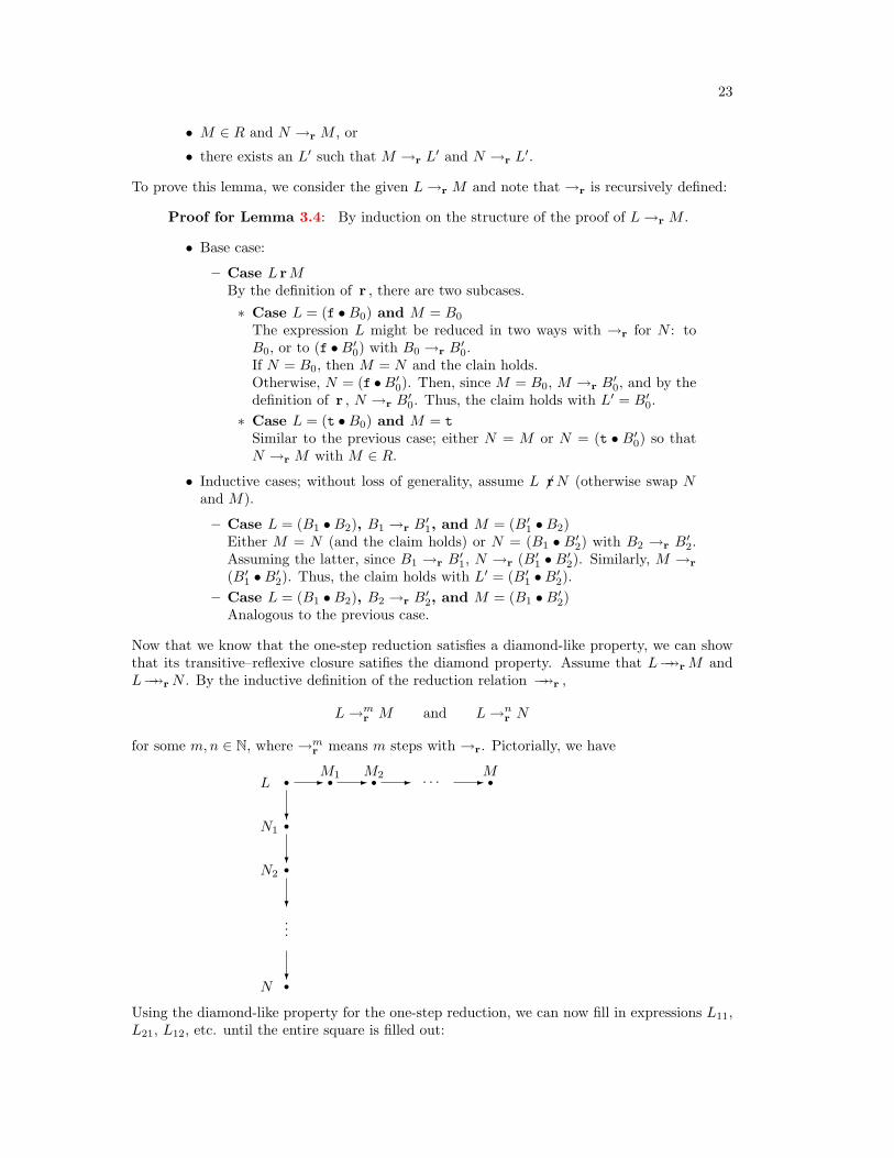
Lemma 3.4 [Diamond-like Property for →r]: If L →r M and L →r N , theneither
• M = N ,
• N ∈ R and M →r N ,
23
• M ∈ R and N →r M , or
• there exists an L′ such that M →r L′ and N →r L′.
To prove this lemma, we consider the given L→r M and note that →r is recursively defined:
Proof for Lemma 3.4: By induction on the structure of the proof of L→r M .
• Base case:
– Case L rMBy the definition of r , there are two subcases.∗ Case L = (f •B0) and M = B0
The expression L might be reduced in two ways with →r for N : toB0, or to (f •B′
0) with B0 →r B′0.
If N = B0, then M = N and the clain holds.Otherwise, N = (f •B′
0). Then, since M = B0, M →r B′0, and by the
definition of r , N →r B′0. Thus, the claim holds with L′ = B′
0.∗ Case L = (t •B0) and M = t
Similar to the previous case; either N = M or N = (t • B′0) so that
N →r M with M ∈ R.
• Inductive cases; without loss of generality, assume L 6 rN (otherwise swap Nand M).
– Case L = (B1 •B2), B1 →r B′1, and M = (B′
1 •B2)Either M = N (and the claim holds) or N = (B1 • B′
2) with B2 →r B′2.
Assuming the latter, since B1 →r B′1, N →r (B′
1 • B′2). Similarly, M →r
(B′1 •B′
2). Thus, the claim holds with L′ = (B′1 •B′
2).– Case L = (B1 •B2), B2 →r B′
2, and M = (B1 •B′2)
Analogous to the previous case.
Now that we know that the one-step reduction satisfies a diamond-like property, we can showthat its transitive–reflexive closure satifies the diamond property. Assume that L→→r M andL→→r N . By the inductive definition of the reduction relation →→r ,
L→mr M and L→n
r N
for some m,n ∈ N, where →mr means m steps with →r. Pictorially, we have
L rN1
rN2
r
M1r M2r?
?
?
- - -
...
?N r
. . . -Mr
Using the diamond-like property for the one-step reduction, we can now fill in expressions L11,L21, L12, etc. until the entire square is filled out:

24 Chapter 3: Consistency of Evaluation
L rN1
rN2
rrL11
-? rL12-
?. . .
. . .rL21
-?
...
...
M1r M2r?
?
?
- - -
...
?N r
. . . -Mr
Formally, this idea can also be cast as an induction.The preceding arguments also show that M =r R if and only if M→→r R. Consequently,
we could have defined the evaluation via reduction without loss of generality. Put differently,symmetric reasoning steps do not help in the evaluation of B expressions. In in the next chapter,however, we will introduce a programming language for which such apparent backward stepscan truly shorten the calculation of the result of a program.
After determining that a program has a unique value, the question arises whether a programalways has a value.
Theorem 3.5: For any B0, evalr(B0) = R0 for some R0.
It follows that an algorithm exists for deciding the equality of B expressions: evaluate bothexpressions and compare the results. Realistic programming languages include arbitrary non-terminating expressions and thus preclude a programmer from deciding the equivalence ofexpressions in this way.
Exercise 3.1. Prove Theorem 3.3 (formally, instead of using a diagram).
Exercise 3.2. Prove Theorem 3.5.

25
Chapter 4: The λ-Calculus
The B language is too restrictive to be useful for any real programming task. Since it has noabstraction capability—i.e., no ability to define functions—it is not remotely as powerful as arealistic programming language.
In this chapter, we study a language called the λ-calculus, which was invented by Church.Although the syntax and reduction relations for the λ-calculus are minimal, it is closely relatedto useful languages like Scheme and ML. In those languages, functions not only manipulatebooleans, integers, and pairs, but also other functions. In other words, functions are values.For example, the map function consumes a function and a list of elements, and applies thefunction to each element of the list. Similarly, a derivative function might take a function(over real numbers) and return a new function that implements its derivative.
In the λ-calculus, the only kind of value is a function, but we will see how other kinds ofvalues (including booleans, integers, and pairs) can be defined in terms of functions.
4.1 Functions in the λ-Calculus
The syntax of the λ-calculus provides a simple, regular method for writing down functions forapplication, and also as the inputs and outputs of other functions. The specification of suchfunctions in the λ-calculus concentrates on the rule for going from an argument to a result,and ignores the issues of naming the function and its domain and range. For example, while amathematician specifies the identity function on some set A as
∀x ∈ A, f(x) = x
or
f :
A −→ Ax 7→ x
in the λ-calculus syntax, we write(λx.x)
An informal reading of the expression (λx.x) says: “if the argument is called x, then the outputof the function is x,” In other words, the function outputs the datum that it inputs.
To write down the application of a function f to an argument a, the λ-calculus uses ordinarymathematical syntax, modulo the placement of parentheses:
(f a)
For example, the expression representing the application of the identity function to a is:
((λx.x) a)
Another possible argument for the identity function is itself:
((λx.x) (λx.x))
Here is an expression representing a function that takes an argument, ignores it, and returnsthe identity function:
(λy.(λx.x))
Here is an expression representing a function that takes an argument and returns a function; thereturned function ignores its own argument, and returns the argument of the original function:
(λy.(λx.y))

26 Chapter 4: The λ-Calculus
The λ-calculus supports only single-argument functions, but this last example shows how afunction can effectively take two arguments, x and y, by consuming the first argument, thenreturning another function to get the second argument. This technique is called currying.
In conventional mathematical notation, f(a) can be “simplified” by taking the expression forthe definition of f , and substituting a everywhere for f ’s formal argument. For example, givenf(x) = x, f(a) can be simplified to a. Simplification of λ-calculus terms is similar: ((λx.x) a)can be simplified to a, which is the result of taking the body (the part after the dot) of (λx.x),and replacing the formal argument x (the part before the dot) with the actual argument a.Here are several examples:
((λx.x) a) → a by replacing x with a in x((λx.x) (λy.y)) → (λy.y) by replacing x with (λy.y) in x((λy.(λx.y)) a) → (λx.a) by replacing y with a in (λx.y)
4.2 λ-Calculus Grammar and Reductions
The general grammar for expressions in the λ-calculus is defined by M (with aliases N and L):
M,N,L = X| (λX.M)| (M M)
X = a variable: x, y, . . .
The following are example members of M :
x (x y) ((x y) (z w))
(λx.x) (λy.(λz.y))
(f(λy.(y y))) ((λy.(y y)) (λy.(y y)))
The first example, x, has no particular intuitive meaning, since x is left undefined. Similarly,(x y) means “x applied to y”, but we cannot say more, since x and y are undefined. Incontrast, the example (λx.x) corresponds to the identity function. The difference between thelast example and the first two is that x appears free in the first two expressions, but it onlyappears bound in the last one.
The relation FV, maps an expression to a set of free variables in the expression. Intuitively,x is a free variable in an expression if it appears outside of any (λx. ). More formally, we definethe relation FV as follows:
FV( X ) = XFV( (λX.M) ) = FV(M) \ XFV( (M1 M2) ) = FV(M1) ∪ FV(M2)
Examples for FV:
FV( x ) = xFV( (x (y x)) ) = x, yFV( (λx.(x y)) ) = yFV( (z (λz.z)) ) = z
Before defining a reduction relation on λ-calculus expressions, we need one more auxilliaryrelation to deal with variable subsitition. The relation [ ← ] maps a source expression, avariable, and an argument expression to a target expression. The target expression is the same

4.2 λ-Calculus Grammar and Reductions 27
as the source expression, except that free instances of the variable are replaced by the argumentexpression:
X1[X1 ←M ] = MX2[X1 ←M ] = X2
where X1 6= X2
(λX1.M1)[X1 ←M2] = (λX1.M1)(λX1.M1)[X2 ←M2] = (λX3.M1[X1 ← X3][X2 ←M2])
where X1 6= X2, X3 6∈ FV(M2)and X3 6∈ FV(M1)\X1
(M1 M2)[X ←M3] = (M1[X ←M3] M2[X ←M3])
Examples for [ ← ]:
x[x← (λy.y)] = (λy.y)z[x← (λy.y)] = z(λx.x)[x← (λy.y)] = (λx.x)(λy.(x y))[x← (λy.y)] = (λz.((λy.y) z)) or (λy.((λy.y) y))(λy.(x y))[x← (λx.y)] = (λz.((λx.y) z))
Finally, to define the general reduction relation n for the λ-calculus, we first define three simplereduction relations, α, β, and η:
(λX1.M) α (λX2.M [X1 ← X2]) where X2 6∈ FV(M)((λX.M1) M2) β M1[X ←M2](λX.(M X)) η M where X 6∈ FV(M)
• The α relation renames a formal argument. It encodes the fact that functions like (λx.x)and (λy.y) are the same function, simply expressed with different names for the argument.
• The β relation is the main reduction relation, encoding function application.
• The η relation encodes the fact that, if a function f takes its argument and immediatelyapplies the argument to g, then using f is equivalent to using g.
The general reduction relation n is the union of α, β, and η:
n = α ∪ β ∪ η
As usual, we define →n as the compatible closure of n, →→n as the reflexive–transitive closureof →n, and =n as the symmetric closure of →→n . We also define →α
n, →βn, and →η
n as thecompatible closures of α, β, and η, respectively. (The compatible closure of α would normallybe written →α, but we use →α
n to emphasize that →n=→αn ∪ →β
n ∪ →ηn.)
Here is one of many possible reductions for ((λx.((λz.z) x)) (λx.x)), where the underlinedportion of the expression is the redex (the part that is reduced by n) in each step:
((λx.((λz.z) x)) (λx.x)) →αn ((λx.((λz.z) x)) (λy.y))→η
n ((λz.z) (λy.y))→β
n (λy.y)
Here is another reduction of the same expression:
((λx.((λz.z) x)) (λx.x)) →βn ((λx.x) (λx.x))
→βn (λx.x)

28 Chapter 4: The λ-Calculus
The parentheses in an expression are often redundant, and they can make large expressionsdifficult to read. Thus, we adopt a couple of conventions for dropping parentheses, plus one fordropping λs:
• Application associates to the left: M1 M2 M3 means ((M1 M2) M3)
• Application is stronger than abstraction: λX.M1M2 means (λX.(M1 M2))
• Consecutive lambdas can be collapsed: λXY Z.M means (λX.(λY.(λZ.M)))
With these conventions, ((λx.((λz.z) x)) (λx.x)) can be abbreviated (λx.(λz.z) x) λx.x, andthe first reduction above can be abbreviated as follows:
(λx.(λz.z) x) λx.x →αn (λx.(λz.z) x) λy.y
→ηn (λz.z) λy.y
→βn λy.y
Exercise 4.1. Reduce the following expressions with →n until no more →βn reductions are
possible. Show all steps.
• (λx.x)
• (λx.(λy.y x)) (λy.y) (λx.x x)
• (λx.(λy.y x)) ((λx.x x) (λx.x x))
Exercise 4.2. Prove the following equivalences by showing reductions.
• (λx.x) =n (λy.y)
• (λx.(λy.(λz.z z) y) x)(λx.x x) =n (λa.a ((λg.g) a)) (λb.b b)
• λy.(λx.λy.x) (y y) =n λa.λb.(a a)
• (λf.λg.λx.f x (g x))(λx.λy.x)(λx.λy.x) =n λx.x
4.3 Encoding Booleans
For the B languages, we arbitrarily chose the symbols f and t to correspond with “false” and“true”, respectively. In the λ-calculus, we make a different choice—which, though arbitrary inprinciple, turns out to be convenient:
true.= λx.λy.x
false.= λx.λy.y
if.= λv.λt.λf.v t f
The .= notation indicates that we are defining a shorthand, or “macro”, for an expression. Themacros for true, false, and if will be useful if they behave in a useful way. For example, wewould expect that
if true M N =n M
for any M and N . We can show that this equation holds by expanding the macros:

4.4 Encoding Pairs 29
if true M N = (λv.λt.λf.v t f) (λx.λy.x) M N→β
n (λt.λf.(λx.λy.x) t f) M N→β
n (λf.(λx.λy.x) M f) N→β
n (λx.λy.x) M N→β
n (λy.M) N→β
n M
Similarly, if false M N =n N :
if false M N = (λv.λt.λf.v t f) (λx.λy.y) M N→β
n (λt.λf.(λx.λy.y) t f) M N→β
n (λf.(λx.λy.y) M f) N→β
n (λx.λy.y) M N→β
n (λy.y) N→β
n N
Actually, it turns out that (if true) =n true and (if false) =n false. In other words, our repre-sentation of true acts like a conditional that branches on its first argument, and false acts likea conditional that branches on its second argument; the if macro is simply for readability.
Exercise 4.3. Show that (if true) =n true and (if false) =n false.
Exercise 4.4. Define macros for binary and and or prefix operators that evaluate in the naturalway with true and false (so that and true false =n false, etc.).
4.4 Encoding Pairs
To encode pairs, we need three operations: one that combines two values, one that extractsthe first of the values, and one that extracts the second of the values. In other words, we needfunctions mkpair, fst, and snd that obey the following equations:
fst (mkpair M N) =n Msnd (mkpair M N) =n N
We will also use the notation 〈M, N〉 as shorthand for the pair whose first element is M andwhose second element is N . One way to find definitions for mkpair, etc. is to consider what a〈M, N〉 value might look like.
Since our only values are functions, 〈M, N〉 must be a function. The function has to containinside it the expressions M and N , and it has to have some way of returning one or the otherto a user of the pair, depending on whether the user wants the first or second element. Thissuggests that a user of the pair should call the pair as a function, supplying true to get the firstelement, or false to get the second one:
〈M, N〉 .= λs.if s M N
As mentioned in the previous section, the if function is really not necessary, and the above canbe simplified by dropping the if.
With this encoding, the fst function takes a pair, then applies it as a function to the argumenttrue:
fst.= λp.p true

30 Chapter 4: The λ-Calculus
Similarly, snd applies its pair argument to false. Finally, to define mkpair, we abstract theabbreviation of 〈M, N〉 over arbitrary M and N .
〈M, N〉 .= λs.s M Nmkpair
.= λx.λy.λs.s x yfst
.= λp.p truesnd
.= λp.p false
Exercise 4.5. Show that mkpair, fst, and snd obey the equations at the beginning of thissection.
4.5 Encoding Numbers
There are many ways to encode numbers in the λ-calculus, but the most popular encoding isdue to Church, and the encoded numbers are therefore called Church numerals. The ideais that a natural number n is encoded by a function of two arguments, f and x, where thefunction applies f to x n times. Thus, the function for 0 takes an f and x and returns x (whichcorresponds to applying f zero times). The function 1 applies f one time, and so on.
0 .= λf.λx.x1 .= λf.λx.f x2 .= λf.λx.f (f x)3 .= λf.λx.f (f (f x))
. . .
The function add1 should take the representation of a number n and produce the representationof a number n + 1. In other words, it takes a 2-argument function and returns another 2-argument function; the new function applies its first argument to the second argument n + 1times. To get the first n applications, the new function can use the old one.
add1.= λn.λf.λx.f (n f x)
Like our encoding of true and false, this encoding of numbers turns out to be convenient. Toadd two numbers n and m, all we have to do is apply add1 to n m times—and m happens tobe a function that will take add1 and apply it m times!
add.= λn.λm.m add1 n
The idea of using the number as a function is also useful for defining iszero, a function thattakes a number and returns true if the number is 0, false otherwise. We can implement iszero byusing a function that ignores its argument and always returns false; if this function is applied0 times to true, the result will be true, otherwise the result will be false.
iszero.= λn.n (λx.false) true
To generalize iszero to number equality, we need subtraction. In the same way that additioncan be built on add1, subtraction can be built on sub1. But, although the add1, add, and iszerofunctions are fairly simple in Church’s number encoding, sub1 is more complex. The numberfunction that sub1 receives as its argument applies a function n times, but the function returnedby sub1 should apply the function one less time. Of course, the inverse of an arbitrary functionis not available for reversing one application.
The function implementing sub1 has two parts:

4.6 Recursion 31
• Pair the given argument x with the value true. The true indicates that an application off should be skipped.
• Wrap the given function f to take pairs, and to apply f only if the pair contains false.Always return a pair containing false, so that f will be applied in the future.
The function wrap wraps a given f :
wrap.= λf.λp.〈false, if (fst p) (snd p) (f (snd p))〉
The function sub1 takes an n and returns a new function. The new function takes f and x,wraps the f with wrap, pairs x with true, uses n on (wrap f) and 〈true, x〉, and extracts thesecond part of the result—which is f applied to x n− 1 times.
sub1.= λn.λf.λx.snd (n (wrap f) 〈true, x〉)
A note on encodings: The encoding for 0 is exactly the same as the encoding for false. Thus,no program can distinguish 0 form false, and programmers must be careful that only true andfalse appear in boolean contexts, etc. This is analogous to the way that C uses the same patternof bits to implement 0, false, and the null pointer.
Exercise 4.6. Show that add1 1 =n 2.
Exercise 4.7. Show that iszero 1 =n false.
Exercise 4.8. Show that sub1 1 =n 0.
Exercise 4.9. Define mult using the technique that allowed us to define add. In other words,implement (mult n m) as n additions of m to 0 by exploiting the fact that n itself applies afunction n times. Hint: what kind of value is (add m)?
Exercise 4.10. The λ-calculus provides no mechanism for signalling an error. What happenswhen sub1 is applied to 0? What happens when iszero is applied to true?
4.6 Recursion
An exercise in the previous section asks you to implement mult in the same way that weimplemented add. Such an implementation exploits information about the way that numbersare encoded by functions.
Given the functions iszero, add, and sub1 from the previous section, we can also implementmult without any knowledge of the way that numbers are encoded (which is the way thatprogrammers normally implement functions). We must define a recursive program that checkswhether the first argument is 0, and if not, adds the second argument to a recursive call thatdecrements the first argument.
mult?.= λn.λm.if (iszero n) 0 (add m (mult (sub1 n) m))
The problem with the above definition of the macro mult is that it refers to itself (i.e., it’srecursive), so there is no way to expand mult to a pure λ-calculus expression. Consequently,the abbreviation is illegal.

32 Chapter 4: The λ-Calculus
4.6.1 Recursion via Self-Application
How can the multiplier function get a handle to itself? The definition of the multipler functionis not available as the mult macro is defined, but the definition is available later. In particular,when we call the multiplier function, we necesarily have a handle to the multiplier function.
Thus, instead of referring to itself directly, the multiplier function could have us supply amultiply function t (itself) as well as arguments to multiply. More precisely, using this strategy,the macro we define is no longer a multiplier function, but a multiplier maker instead: it takessome function t then produces a multiplier function that consumes two more arguments tomultiply:
mkmult0.= λt.λn.λm.if (iszero n) 0 (add m (t (sub1 n) m))
This mkmult0 macro is well defined, and (mkmult0 t) produces a multiplication function. . .assuming that t is a multiplication function! Obviously, we still do not have a multiplicationfunction. We tried to parameterize the original mult definition by itself, but in doing so we lostthe mult definition.
Although we can’t supply a multiplication function as t, we could instead supply a multi-plication maker as t. Would that be useful, or do we end up in an infinite regress? As it turnsout, supplying a maker to a maker can work.
Assume that applying a maker to a maker produces a multiplier. Therefore, the initialargument t to a maker will be a maker. In the body of the maker, wherever a multiplier isneeded, we use (t t)—because t will be a maker, and applying a maker to itself produces amultiplier. Here is a maker, mkmult1 that expects a maker as its argument:
mkmult1.= λt.λn.λm.if (iszero n) 0 (add m ((t t) (sub1 n) m))
If mkmulti1 works, then we can get a mult function by applying mkmulti1 to itself:
mult.= (mkmult1 mkmult1)
Let’s try this suspicious function on 0 and m (for some arbitrary m) to make sure that we get0 back. We’ll expand abbreviations only as necessary, and we’ll assume that abbreivations likeiszero and 0 behave in the expected way:
mult 0 m= (mkmult1 mkmult1) 0 m→n (λn.λm.if (iszero n) 0 (add m ((mkmult1 mkmult1) (sub1 n) m))) 0 m→n (λm.if (iszero 0) 0 (add m ((mkmult1 mkmult1) (sub1 0) m))) m→n if (iszero 0) 0 (add m ((mkmult1 mkmult1) (sub1 0) m))→→n if true 0 (add m ((mkmult1 mkmult1) (sub1 0) m))→→n 0
So far, so good. What if we multiply n and m, for some n 6= 0?
mult n m= (mkmult1 mkmult1) n m→n (λn.λm.if (iszero n) 0 (add m ((mkmult1 mkmult1) (sub1 n) m))) n m→n (λm.if (iszero n) 0 (add m ((mkmult1 mkmult1) (sub1 n) m))) m→n if (iszero n) 0 (add m ((mkmult1 mkmult1) (sub1 n) m))→→n if false 0 (add m ((mkmult1 mkmult1) (sub1 n) m))→→n (add m ((mkmult1 mkmult1) (sub1 n) m))

4.6 Recursion 33
Since mult = (mkmult1 mkmult1), the last step above can also be written as (add m (mult (sub1 n) m)).Thus,
mult 0 m →→n 0mult n m →→n (add m (mult (sub1 n) m)) if n 6= 0
This is exactly the relationship we want among mult, add, sub1, and 0.
Exercise 4.11. Define a macro mksum such that (mksum mksum) acts like a “sum” functionby consuming a number n and adding all the numbers from 0 to n.
4.6.2 Lifting Out Self-Application
The technique of the previous section will let us define any recursive function that we want.It’s somewhat clumsy, though, because we have to define a maker function that applies aninitial argument to itself for every recursive call. For convenience, we would like to pull theself-application pattern out into its own abstraction.
More concretely, we want a function, call it mk, that takes any maker like mkmult0 andproduces a made function. For example, (mk mkmult0) should be a multiplier.
mk?.= λt.t (mk t)
The mk definition above is ill-formed, but we can start with this bad definition to get the idea.The mk function is supposed to take a maker, t, and produce a made function. It does soby calling the function-expecting maker with (mk t) — which is supposed to create a madefunction.
We can fix the circular mk definition using the technique of the previous section:
mkmk.= λk.λt.t ((k k) t)
mk.= (mkmk mkmk)
We can check that (mk mkmult0) behaves like mult:
(mk mkmult0) 0 m= ((mkmk mkmk) mkmult0) 0 m= (((λk.λt.t ((k k) t)) mkmk) mkmult0) 0 m→n ((λt.t ((mkmk mkmk) t) mkmult0) 0 m→n (mkmult0 ((mkmk mkmk) mkmult0)) 0 m→n (λn.λm.if (iszero n) 0 (add m (((mkmk mkmk) mkmult0) (sub1 n) m))) 0 m→n (λm.if (iszero 0) 0 (add m (((mkmk mkmk) mkmult0) (sub1 0) m))) m→n if (iszero 0) 0 (add m (((mkmk mkmk) mkmult0) (sub1 0) m))→→n 0
(mk mkmult0) n m= ((mkmk mkmk) mkmult0) n m= (((λk.λt.t ((k k) t)) mkmk) mkmult0) n m→n ((λt.t ((mkmk mkmk) t) mkmult0) n m→n (mkmult0 ((mkmk mkmk) mkmult0)) n m→n (λn.λm.if (iszero n) 0 (add m (((mkmk mkmk) mkmult0) (sub1 n) m))) 0 m→n (λm.if (iszero n) 0 (add m (((mkmk mkmk) mkmult0) (sub1 n) m))) m→n if (iszero n) 0 (add m (((mkmk mkmk) mkmult0) (sub1 n) m))→→n (add m (((mkmk mkmk) mkmult0) (sub1 n) m))= (add m ((mk mkmult0) (sub1 n) m))

34 Chapter 4: The λ-Calculus
4.6.3 Fixed Points and the Y Combinator
The mk function should seem somewhat mysterious at this point. Somehow, it makes mkmult0useful, even though mkmult0 can only make a multiplier when it is given the multiplier that itis supposed to make!
In general, mkmult0 might be given any function, and the resulting “multiplier” that itreturns would behave in many different ways for many different input functions, and the outputfunction would typically be quite different from the input function. But mk somehow managesto pick an input function for mkmult0 so that the output function is the same as the inputfunction. In other words, mk finds the fixed point of mkmult0.
As it turns out, mk can find the fixed point of any function. In other words, if applying mkto M produces N , then applying M to N simply produces N again.
Theorem 4.1: M (mk M) =n (mk M) for any M
Proof for Theorem 4.1: Since =n is the symmetric closure of →→n , we canprove the claim by showing that mk M→→n M (mk M):
mk M = (mkmk mkmk) M= ((λk.λt.t ((k k) t)) mkmk) M→n (λt.t ((mkmk mkmk) t) M→n M ((mkmk mkmk) M)= M (mk M)
A function that behaves like mk is called a fixed-point operator. The mk function is onlyone of many fixed-point operators in the λ-calculus. The more famous one is called Y:1
Y.= λf.(λx.f (x x)) (λx.f (x x))
In general, Y lets us define recursive functions more easily than the manual technique of Sec-tion 4.6.1. For example, we can define sum as
sum.= Y (λs.λn.if (iszero n) 0 (add n (s (sub1 n))))
Since we do not have to repeat a large maker expression, we can skip the intermediate makerabbreviations mksum, and instead apply Y directly to a maker function.
In addition, a programmer who sees the above definition of sum will immediately note the Y,see that s is the argument of Y’s argument, and then read λn . . . as the definition of a recursivefunction named s.
Exercise 4.12. Prove that M (Y M) =n (Y M) for any M .
Exercise 4.13. Define an encoding for Lisp cons cells, consisting of the following macros:
• null, a constant
• cons, a function that takes two arguments and returns a cons cell
• isnull, a function that returns true if its argument is null, false if it is a cons cell
• car, a function that takes a cons cell and returns its first element
• cdr, a function that takes a cons cell and returns its second element
1The term Y combinator actually refers to the whole family of fixed-point operators. More on this later.

4.7 Facts About the λ-Calculus 35
In particular, your encoding must satisfy the following equations:
(isnull null) =n true(isnull (cons M N)) =n false(car (cons M N)) =n M(cdr (cons M N)) =n N
Your encoding need not assign any particular meaning to expressions such as (car null) or(car cons).
Exercise 4.14. Using your encoding from the previous exercise, define length, which takes alist of booleans and returns the number of cons cells in the list. A list of booleans is either null,or (cons b l) where b is true or false and l is a list of booleans.
4.7 Facts About the λ-Calculus
When is an expression fully reduced? Almost any expression can be reduced by →αn, which
merely renames variables, so it shouldn’t count in the definition. Instead, a fully reducedexpression is one that cannot be reduced via →β
n or →ηn.
An expression is a normal form if it cannot be reduced by →βn or →η
n.
M has normal form N if M =n N and N is a normal form.
A normal form acts like the result of a λ-calculus expression. If an expression has a normal form,then it has exactly one normal form (possibly via many different reductions). More precisely,there is one normal form modulo →α
n renamings.
Theorem 4.2 [Normal Forms]: If L =n M , L =n N , and both M and N arenormal forms, then M =α N .
As usual, =α is the equivalence generated by the compatible closure of α. Theorem 4.2 is easyto prove given the Church-Rosser property for the λ-calculus:
Theorem 4.3 [Church-Rosser for =n]: If M =n N , then there exists an L′ suchthat M→→n L′ and N→→n L′.
As for =r, then proof of this theorem hinges on the diamond property for →→n .
Theorem 4.4 [Diamond Property for →→n ]: If L→→r M and L→→r N , thenthere exists an expression L′ such that M→→r L′ and N→→r L′.
The one-step relation →n does not obey the diamond property, or even a slightly contortedone, such as the diamond-like property of →r. The reason is that →β
n can duplicate reducibleexpressions. For example:
(λx.x x) ((λy.y) (λz.z))
HHHHH
Hj
(((λy.y) (λz.z))((λy.y) (λz.z)))
(λx.x x) (λz.z)

36 Chapter 4: The λ-Calculus
There’s no single step that will bring both of the bottom expressions back together. As we’llsee in the next chapter, the way around this problem is to define a notion of parallel reductionson independent subexpression, so that both ((λy.y) (λz.z)) sub-expressions on the left can bereduced at once. For now, though, we will not try to prove Theorem 4.4. Instead, we willdemonstrate the diamond property for a related language in the next chapter.
Unlike expressions in B, where every expression has a result f or t, not every λ-calculusexpression has a normal form. For example, Ω has no normal form:
Ω .= ((λx.x x) (λx.x x))
Even if an expression has a normal form, then there may be an inifite reduction sequence forthe expression that never reaches a normal form. For example:
(λy.λz.z)((λx.x x) (λw.w w))→n λz.z normal form
(λy.λz.z)((λx.x x) (λw.w w))→n (λy.λz.z)((λw.w w) (λw.w w))→n (λy.λz.z)((λw.w w) (λw.w w))→n . . . same expression forever
Thus, Theorem 4.2 guarantees that at most once normal form exists, but we do not yet have away to find it. Intuitively, the problem with the non-terminating reduction above is that we areevaluating the argument of a function that will not be used in the function body. This suggestsa strategy where we apply the leftmost β or η reduction in an expression to reach a normalform:
M →n N if M β NM →n N if M η N(M N)→n (M ′ N) if M →n M ′
and ∀L, (M N) 6β L and (M N) 6η L(M N)→n (M N ′) if N →n N ′
and M is in normal formand ∀L, (M N) 6β L and (M N) 6η L
The→n relation is the normal order reduction relation, and it is guaranteed to find a normalform if one exists.
Theorem 4.5 [Normal Order Reduction]: M has normal form N if and onlyif M→→n N .
Normal-order reduction is also called call-by-name.Although a normal-order reduction always finds a normal form if it exists, practically no
programming language uses this form of reduction. The reason is that normal order, while ispowerful, is often slow. For example, in the previous diagram showing the non-diamondness of→n, the reduction on the left corresponds to normal order, but the reduction on the right willproduce the identity function in fewer steps.
In any case, since we have a notion of unique normal form (modulo α-renaming), a naturalquestion to ask is whether we can define an evaln in the same way as evalr:
evaln(M) ?= N if M =n N and N is a normal form
The above definition is imprecise with respect to α-renaming, but there is a deeper problem.As we have seen, there are functions like mk and Y that behave in the same way, but cannotbe reduced to each other. In the next chapter, we will look at a way to resolve this problem.
Exercise 4.15. Prove that ((λx.x x) (λx.x x)) has no normal form.

4.8 History 37
4.8 History
Church invented the lambda calculus slightly before Turning invented Turing machines.Barendregt [2] provides a comprehensive study of Church’s λ-calculus as a logical system,
and many conventions for the treatment of terms originate with Barendregt. His book providesnumerous techniques applicable to the calculus, though it does not cover λ-calculus as a calculusfor a programming language.

38 Chapter 4: The λ-Calculus

Part II
Models of Realistic Languages
39

41
Chapter 5: ISWIM
Church developed the λ-calculus as a way of studying all of mathematics, as opposed to me-chanical computation specifically. In the 1960’s Landin showed that Church’s calculus was,in fact, not quite an appropriate model of most programming languages. For example, theλ-calculus expression
(λx.1) (sub1 λy.y)
reduces to (the encoding of) 1, even though most languages would instead complain about(sub1 λy.y). The problem is not just in the encoding of sub1 and λy.y, but that a β reductionon the entire expression can ignore the argument (sub1 λy.y) completely.
Whether such call-by-name behavior is desirable or not is open to debate. In any case,many languages do not support call-by-name. Instead, they support call-by-value, where thearguments to a function must be fully evaluated before the function is applied.
In this chapter, we introduce Landin’s ISWIM, which more closely models the core of call-by-value languages such as Scheme and ML. The basic syntax of ISWIM is the same as for theλ-calculus, and the notions of free variables and substition are the same. Unlike the λ-calculus,and more like real programming languages, ISWIM comes with a set of basic constants andprimitive operations. But the more fundamental difference is in ISWIM’s call-by-value reductionrules.
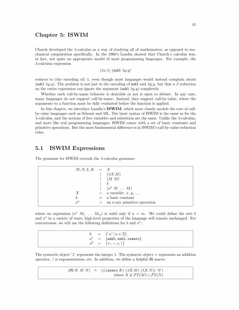
5.1 ISWIM Expressions
The grammar for ISWIM extends the λ-calculus grammar:
M,N,L,K = X| (λX.M)| (M M)| b| (on M . . . M)
X = a variable: x, y, . . .b = a basic constanton = an n-ary primitive operation
where an expression (on M1 . . . Mm) is valid only if n = m. We could define the sets band on in a variety of ways; high-level properties of the language will remain unchanged. Forconcreteness, we will use the following definitions for b and on:
b = dne |n ∈ Zo1 = add1, sub1, iszeroo2 = +,−, ∗, ↑
The syntactic object d1e represents the integer 1. The syntactic object + represents an additionoperator, ↑ is exponentiation, etc. In addition, we define a helpful if0 macro:
(if0 K M N) .= (((iszero K) (λX.M) (λX.N)) d0e)where X 6∈ FV(M) ∪ FV(N)
42 Chapter 5: ISWIM
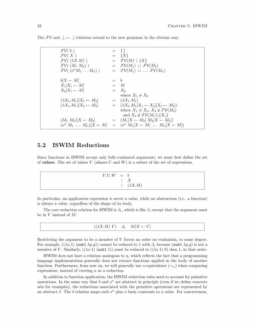
The FV and [ ← ] relations extend to the new grammar in the obvious way:
FV( b ) = FV( X ) = XFV( (λX.M) ) = FV(M) \ XFV( (M1 M2) ) = FV(M1) ∪ FV(M2)FV( (onM1 . . .Mn) ) = FV(M1) ∪ . . . FV(Mn)
b[X ←M ] = bX1[X1 ←M ] = MX2[X1 ←M ] = X2
where X1 6= X2
(λX1.M1)[X1 ←M2] = (λX1.M1)(λX1.M1)[X2 ←M2] = (λX3.M1[X1 ← X3][X2 ←M2])
where X1 6= X2, X3 6∈ FV(M2)and X3 6∈ FV(M1)\X1
(M1 M2)[X ←M3] = (M1[X ←M3] M2[X ←M3])(on M1 . . . Mn)[X ←M ] = (on M1[X ←M ] . . . Mn[X ←M ])
5.2 ISWIM Reductions
Since functions in ISWIM accept only fully-evaluated arguments, we must first define the setof values. The set of values V (aliases U and W ) is a subset of the set of expressions.
V,U,W = b| X| (λX.M)
In particular, an application expression is never a value, while an abstraction (i.e., a function)is always a value, regardless of the shape of its body.
The core reduction relation for ISWIM is βv, which is like β, except that the argument mustbe in V instead of M :
((λX.M) V ) βv M [X ← V ]
Restricting the argument to be a member of V forces an order on evaluation, to some degree.For example, ((λx.1) (sub1 λy.y)) cannot be reduced to 1 with βv because (sub1 λy.y) is not amember of V . Similarly, ((λx.1) (sub1 1)) must be reduced to ((λx.1) 0) then 1, in that order.
ISWIM does not have a relation analogous to η, which reflects the fact that a programminglanguage implementation generally does not extract functions applied in the body of anotherfunction. Furthermore, from now on, we will generally use α-equivalence (=α) when comparingexpressions, instead of viewing α as a reduction.
In addition to function application, the ISWIM reduction rules need to account for primitiveoperations. In the same way that b and on are abstract in principle (even if we define concretesets for examples), the reductions associated with the primitive operations are represented byan abstract δ. The δ relation maps each on plus n basic constants to a value. For concreteness,

5.3 The Yv Combinator 43
we choose the following δ:
(add1 dme) b1 dm + 1e
(sub1 dme) b1 dm− 1e
(iszero d0e) b1 λxy.x(iszero dne) b1 λxy.y n 6= 0
(+ dme dne) b2 dm + ne
(− dme dne) b2 dm− ne
(∗ dme dne) b2 dm · ne
(↑ dme dne) b2 dmne
δ = b1 ∪ b2
By combining β and δ, we arrive at the complete reduction relation v:
v = βv ∪ δ
As usual, →v is the compatible closure of v, →→v is the reflexive–transitive closure of→v, and=v is the symmetric closure of →→v .
Exercise 5.1. Show a reduction of
(λw.(− (w d1e) d5e)) ((λx.x d10e) λyz.(+ z y))
to a value with →v.
5.3 The Yv Combinator
For the pure λ-calculus, we defined a function Y that finds a fixed point of any expression,and can therefore be used to define recursive functions. Although it’s stilll true in ISWIM that(f (Y f)) is the same as (Y f) for any f , this fact does not turn out to be useful:
Y f = (λf.(λx.f (x x)) (λx.f (x x))) f→v (λx.f (x x)) (λx.f (x x))→v f ((λx.f (x x)) (λx.f (x x)))
The problem is that the argument to f in the outermost application above is not a value—andcannot be reduced to a value—so (Y f) never produces the promised fixed-point function.
We can avoid the infinite reduction by changing each application M within Y to (λX.M X),since the application is supposed to return a function anyway. This inverse-η transformationputs a value in place of an infinitely reducing application. The final result is the Yv combinator:
Yv = (λf.(λx.
( (λg. (f (λx. ((g g) x))))(λg. (f (λx. ((g g) x)))) x)))
The Yv combinator works when applied to a function that takes a function and returns anotherone.
Theorem 5.1 [Fixed-Point Theorem for Yv]: If K = λgx.L, then (K (Yv K)) =v
(Yv K).

44 Chapter 5: ISWIM
Proof for Theorem 5.1: The proof is a straightforward calculation where all ofthe basic proof steps are βv steps:
(Yv K)= ((λf.λx.((λg.(f (λx.((g g) x)))) (λg.(f (λx.((g g) x)))) x)) K)→v λx.(((λg.(K (λx.((g g) x)))) (λg.(K (λx.((g g) x))))) x)→v λx.((K (λx.(((λg.(K (λx.((g g) x)))) (λg.(K (λx.((g g) x))))) x))) x)→v λx.(((λgx.L) (λx.(((λg.(K (λx.((g g) x)))) (λg.(K (λx.((g g) x))))) x))) x)→v λx.((λx.L[g ← (λx.(((λg.(K (λx.((g g) x)))) (λg.(K (λx.((g g) x))))) x))]) x)→v λx.L[g ← (λx.((λg.(K (λx.((g g) x)))) (λg.(K (λx.((g g) x)))) x))]v← ((λgx.L) (λx.((λg.(K (λx.((g g) x)))) (λg.(K (λx.((g g) x)))) x)))= (K (λx.((λg.(K (λx.((g g) x)))) (λg.(K (λx.((g g) x)))) x)))
v← (K (Yv K))
The proof of Theorem 5.1 looks overly complicated because arguments to procedures must bevalues for βv to apply. Thus instead of calculating
λx.((K (λx.(((λg.(K (λx.((g g) x)))) (λg.(K (λx.((g g) x))))) x))) x)= λx.((K (Yv K)) x)= λx.((λgx.L) (Yv K)) x)
we need to carry around the value computed by (Yv K). To avoid this complication in thefuture, we show that an argument that is provably equal to a value (but is not necessarily avalue yet) can already be used as if it were a value for the purposes of =v.
Theorem 5.2: If M =v V , then for all (λX.N), ((λX.N) M) =v N [X ←M ].
Proof for Theorem 5.2: The initial portion of the proof is a simple calculation:
((λX.N) M) =v ((λX.N) V ) =v N [X ← V ] =v N [X ←M ]
The last step in this calculation, however, needs a separate proof by induction onN , showing that N [X ←M ] =v N [X ← L] if M =v L:
• Base cases:– Case N = b
b[X ←M ] = b =v b = b[X ← L].– Case N = Y
If Y = X, then X[X ← M ] = M =v L = X[X ← L]. Otherwise,Y [X ←M ] = Y =v Y = Y [X ← L].
• Inductive cases:– Case N = (λY.N ′)
If Y = X, then N [M ← X] = N =v N = N [L ← X]. Otherwise, byinduction, N ′[X ←M ] =v N ′[X ← L]. Then,
(λY.N ′)[X ←M ]= (λY.N ′[X ←M ])=v (λY.N ′[X ← L])= (λY.N ′)[X ← L]
– Case N = (N1 N2)By induction, Ni[X ←M ] =v Ni[X ← L] for i ∈ [1, 2]. Then,
(N1 N2)[X ←M ]= (N1[X ←M ] N2[X ←M ])=v (N1[X ← L] N2[X ← L])= (N1N2)[X ← L]

5.4 Evaluation 45
– Case N = (on N1 . . . Nn)Analogous to the previous case.
5.4 Evaluation
For defining an evaluator, functions as values pose just as much of a problem for ISWIM as forthe λ-calculus. For example, the expression
(λx.x) (λy.(λx.x) d0e)
is clearly equivalent to bothλy.(λx.x) d0e
andλy.d0e
Which one should we pick as the result of an evaluator? While all of these results hopefullyrepresent one and the same function, it is also clear that there are infinitely many ways torepresent a function. We therefore adopt a solution that essentially all practical programmingsystems implement: when a program reduces to a function value, the evalv function merelyreturns a token indicating that the value is a function.
We define A to be the set of results for evaluating ISWIM functions:
A = b ∪ function
The partial function evalv is defined as follows:
evalv(M) =
b if M =v bfunction if M =v λX.N
If evalv(M) does not exist, we say that M diverges. For example, Ω diverges.
Exercise 5.2. Suppose that we try to strengthen the evaluation function as follows:
eval1(M) =
b if M =v bfunction1 if M =v λX.N N 6= λY.N ′ for any Y, N ′
function+ if M =v λX.λY.N
Is eval1 a function? If so, prove it. If not, provide a counter-example.
5.5 Consistency
The definition of ISWIM’s evaluator relies on an equational calculus for ISWIM. Although thecalculus is based on intuitive arguments and is almost as easy to use as a system of arithmetic, itis far from obvious whether the evaluator is a function that always returns a unique answer fora program. But for a programmer who needs a deterministic, reliable programming language,this fact is crucial and needs to be established formally. In short, we need to modify theconsistency theorem of evalr for ISWIM’s evalv. The proof of this theorem turns out to be farmore complex than the one for evalr, though it follows the same outline.
We start with the basic theorem asserting the Church-Rosser property for ISWIM’s calculus.
Theorem 5.3 [Consistency of evalv]: The relation evalv is a partial function.

46 Chapter 5: ISWIM
Proof for Theorem 5.3: Assume that the Church-Rosser Property holds: ifM =v N then there exists an expression L such that M→→v L and N→→v L.
Let evalv(M) = A1 and evalv(M) = A2 for answers A1 and A2. We need to showthat A1 = A2. Based on the definition of ISWIM answers, we distinguish two cases:
• Case A1 ∈ b, A2 ∈ bIt follows from Church-Rosser that two basic constants are provably equal ifand only if they are identical, since neither is reducible.
• Case A1 = function, A2 ∈ bBy the definition of evalv, M =v A2 and M =v λx.N for some N , so A2 =v
λx.N . Again by Church-Rosser and the irreducibility of constants, λx.N→→v A2.But by definition of the reduction relation →→v , λx.N→→v K implies thatK = λx.K ′. Thus it is impossible that λx.N reduces to A2, which means thatthe assumptions of the case are contradictory.
• Case A1 ∈ b, A2 = functionAnalogous to the previous case.
• Case A1 = function, A2 = functionThen A1 = A2.
These are all possible cases, and hence, it is always true that A1 = A2, so evalv isa function.
By the preceding proof, we have reduced the consistency property to the Church-Rosser propertyfor ISWIM.
Theorem 5.4 [Church-Rosser for ISWIM]: If M =v N , then there exists anexpression L such that M→→v L and N→→v L.
Proof for Theorem 5.4: The proof is essentially a replica of the proof for =r
(Theorem 3.2). It assumes a diamond property for the reduction relation →→v .
After disposing of the Consistency and Church-Rosser theorems, we have arrived at the core ofthe problem. Now we need to show the diamond property for ISWIM.
Theorem 5.5 [Diamond Property for →→v ]: If L→→v M and L→→v N , thenthere exists an expression K such that M→→v K and N→→v K.
For →→r , a diamond-like property holds for the single-step relation→r, from which the diamondproperty for the transitive closure easily follows. But, analogous to the example in the previouschapter, it is clear that the diamond property cannot hold for →v. The βv reduction can copyredexes in the argument of a function, which prevents the existence of the common contractumin certain diamonds. For an example, consider the expression
((λx.(x x)) (λy.((λx.x) (λx.x))))
which contains the two overlapping and underlined βv-redexes. By one or the other of one ofthem, we get the expressions
((λx.(x x)) (λy.(λx.x)))
and((λy.((λx.x) (λx.x))) (λy.((λx.x) (λx.x))))
Both expressions contain redexes, but as the following diagram shows, the one-step reductionsstarting from these expressions do not lead to a common expression.

5.5 Consistency 47
((λx.(x x))(λy.((λx.x)(λx.x))))
HHHH
HHj
((λy.((λx.x)(λx.x)))(λy.((λx.x)(λx.x))))
((λx.(x x))(λy.(λx.x)))
?
HHHHHH
HHHHHHj
(λy.((λx.x)(λx.x)))
((λy.(λx.x))(λy.((λx.x)(λx.x))))
((λy.((λx.x)(λx.x))))(λy.(λx.x))
?
((λy.(λx.x))(λy.(λx.x))
Hence, the one-step relation →v does not satisfy the diamond property.Since the problem of the one-step relation based on v is caused by reductions that duplicate
redexes, we consider an extension →v of the one-step reduction →v that contracts severalnon-overlapping redexes in parallel. If this extension satisfies the diamond property, and if itstransitive–reflexive closure is the same as that of →v, then we can prove the diamond propertyfor the →→v reduction.
The parallel extension →v is defined as follows:
M →v N if M =α N(on b1 . . . bn) →v δ(on, b1, . . . bn) if δ(on, b1, . . . bn) is defined((λX.M) N) →v M ′[X ← V ] if M →v M ′ and N →v V(M N) →v (M ′ N ′) if M →v M ′ and N →v N ′
(λX.M) →v (λx.M ′) if M →v M ′
(on M1 . . . Mn) →v (on M ′1 . . . M ′
n) if Mi →v M ′i , i ∈ [1, n]
This relation satisfies the diamond property.
Theorem 5.6 [Diamond Property for →v]: If L →v M and L →v N , thenthere exists an expression K such that M →v K and N →v K.
Proof for Theorem 5.6: By induction on the structure of the proof tree ofL →v M .
• Base cases:
– Case L =α MSet K = N , and the claim holds.
– Case L = (on b1 . . . bn),M = δ(on, b1, . . . bn)Since δ is a function there is no other possible reduction for L; set K =N = M .
• Inductive cases:
– Case L = ((λX.M0) L1), M = M ′0[X ← V ], M0 →v M ′
0, L1 →v VThere are two possiblities for the reduction path L →v N . Either the twoparts of the application merely reduce separately, or the application is alsoreduced via βv:

48 Chapter 5: ISWIM
∗ Case L = ((λX.M0) L1), N = ((λX.M ′′0 ) L′′1), M0 →v M ′′
0 , L1 →v
L′′1In this case, M0, M ′
0, and M ′′0 satisfy the antecedent of the inductive
hypothesis, and so do L1, V , and L′′1 . Hence, there are expressionsK0 and K1 that complete the upper half of these two diamons. If wealso knew that substitution and parallel reduction commute, we couldconclude that K = K0[X ← K1], since ((λX.M ′′
0 ) L′′1) →v K0[X ←K1] and M ′
0[X ← V ] →v K ′[X ← K1].∗ Case L = ((λX.M0) L1), N = M ′′
0 [X ← V ′], M0 →v M ′′0 , L1 →v V ′
As in the first subcase, M0, M ′0, and M ′′
0 and L1, V , and V ′′ determineupper halves of diamonds. By the induction hypothesis, each yields twolower halves of diamonds and related terms K0 and K1. And again, ifsubstitution and parallel reduction commute, setting K = K0[X ← V ]concludes the subcase.
To complete this case, we are obliged to prove the commutation property.We postpone this proof, since other cases also depend on it; see Lemma 5.7.
– Case L = (L1 L2), M = (M1 M2), Li →v Mi
Analogous to the previous case.– Case L = (on L1 . . . Ln), M = (on M1 . . .Mn), Li →v Mi
There are two cases:∗ Case L1 = b1, . . . Ln = bn, N = δ(on, b1, . . . bn)
Then M = L and K = N .∗ Case N = (on N1 . . . Nn), Li →v Ni
An n-fold use of the inductive hypothesis yields the conclusion.– Case L = (λX.L0), M = (λX.M0), L0 →v M0
The only possibility for N is N = (λX.N0) with L0 →v N0. The inductionhypothesis applies to L0,M0, and N0 and yields an expression K0; K =(λX.K0).
To finish the preceding proof, we need to show that substitutions in expressions that are relatedby parallel reduction do not affect the reduction step.
Lemma 5.7: If M →v M ′ and N →v N ′ then M [X ← N ] →v M ′[X ← N ′].
Proof for Lemma 5.7: By induction on the proof tree of M →v M ′:
• Base cases:– Case M =α M ′
In this special case, the claim essentially says that if N →v N ′, thenM [X ← N ] →v M [X ← N ′]. The proof of this specialized claim is aninduction on the structure of M . We leave this proof as an exercise.
– Case M = (on b1 . . . bn), M ′ = δ(on, b1, . . . , bn)M and M ′ are closed, so M [X ← N ] = M and M ′[X ← N ] = M ′, andwe know already that M →v M ′.
• Inductive cases:– Case M = ((λX0.M0) L0), M ′ = M ′
0[X0 ← V ], M0 →v M ′0, L0 →v V
By induction, M0[X ← N ] →v M ′0[X ← N ′] and L0[X ← N ] →v V [X ←
N ′]. Thus:
M [X ← N ] = ((λX0.M0[X ← N ]) L0[X ← N ])→v M ′
0[X ← N ′][X0 ← V [X ← N ′]]= M ′
0[X0 ← V ][X ← N ′] (†)=α M ′[X ← N ′]

5.6 Observational Equivalence 49
Equation (†) is a basic property of the substitution function. We leave thisstep as an exercise.
– Case M = (M1 M2), M ′ = (M ′1 M ′
2), Mi →v M ′i
By induction, Mi[X ← N ] →v M ′i [X ← N ′] for both i = 1 and i = 2.
Thus,M [X ← N ] = (M1[X ← N ] M2[X ← N ])
→v (M ′1[X ← N ] M ′
2[X ← N ])→v (M ′
1[X ← N ′] M ′2[X ← N ′])
= (M ′1 M ′
2)[X ← N ′]= M ′[X ← N ′]
So the claim holds.– Case M = (on M1 . . . Mn), M ′ = (on M ′
1 . . . M ′n), Mi →v M ′
i
Analogous to the previous case.– Case M = (λX.M0), M ′ = (λX.M ′
0) M0 →v M ′0
Analogous to the previous case.
Exercise 5.3. Prove that if N →v N ′, then M [X ← N ] →v M [X ← N ′].
Exercise 5.4. Prove that if X 6∈ FV(L) then
K[X ← L][X ′ ←M [X ← L]] =α K[X ′ ←M ][X ← L]
Exercise 5.5. Prove that the transitive–reflexive closure of the parallel reduction →v is thesame as →→v . This fact, along with Theorem 5.6, supports the proof of Theorem 5.5.
5.6 Observational Equivalence
Besides program evaluation, the transformation of programs plays an important role in thepractice of programming and in the implementation of programming languages. For example, ifM is a procedure, and if we think that N is a procedure that can perform the same computationas M but faster, then we would like to know whether M is really interchangeable with N . Forone special instance of this problem, ISWIM clearly provides a solution: if both expressions arecomplete programs and we know that M =v N , then evalv(M) = evalv(N) and we know thatwe can replace M by N .
In general, however, M and N are sub-expressions of some program, and we may not beable to evaluate them independently. Hence, what we really need is a general relation thatexplains when expressions are “equivalent in functionality”.
To understand the notion of “equivalent in functionality”, we must recall that the userof a program can only observe the output, and is primarily interested in the output. Theprogrammer usually does not know the text of the program or any aspects of the text. In otherwords, such an observer treats programs as black boxes that produce some value in an unknownmanner. It is consequently natural to say that the effect of an expression is the effect it haswhen it is a part of a program. Going even further, the comparison of two open expressionsreduces to the question whether there is a way to tell apart the effects of the expressions.Or, put positively, if two expressions have the same effect, they are interchangeable from thestandpoint of an external observer.
Before we continue, we need a notion of expressions contexts. The following grammar Cdefines a set of near-expressions. They are not quite expressions, because each member of C

50 Chapter 5: ISWIM
contains a hole, written [ ], in the place of one subexpression.
C = [ ]| (λX.C)| (C M)| (M C)| (on M . . . M C M . . . M)
C[M ] means “replace the [ ] in C with M”
For example, (λx.[ ]) and (+ 1 ((λx.d0e) [ ])) are members of C, and
(λx.[ ])[(λy.x)] = (λx.(λy.x))(+ 1 ((λx.d0e) [ ]))[(z d12e)] = (+ 1 ((λx.d0e) (z d12e)))
Unlike substitution, filling a context hole can capture variables.With this definition of context, we can express the notion of observational equivalence. Two
expressions M and N are observationally equivalent, written M 'v N , if and only if theyare indistinguishable in all contexts C.
M 'v N if evalv(C[M ]) = evalv(C[N ]) for all C
The definition implies that if M 'v N , then evalv(C[M ]) and evalv(C[N ]) must be either bothdefined or both undefined for any given C.
Observational equivalence obviously extends program equivalence in terms of evalv; if pro-grams M and N are observationally equivalent, then they are programs in the empty context, soevalv(M) = evalv(N). But this is also the least we should expect from a theory of expressionswith equivalent functionality. As the name already indicates, observational equivalence is anequivalence relation. Finally, if two expressions are observationally equivalent, then embeddingthe expressions in contexts should yield observationally equivalent expressions. After all, theadded pieces are identical and should not affect the possible effects of the expressions on theoutput of a program. In short, observational equivalence is a congruence relation, i.e., itsclosure over contexts is also an equivalence relation.
Theorem 5.8: For any expressions M , N , and L,
1. M 'v M ;
2. if L 'v M and M 'v N , then L 'v N ;
3. if L 'v M , then M 'v L; and
4. if M 'v N , then C[M ] 'v C[N ] for all contexts C.
Proof for Theorem 5.8: Points 1 through 3 are trivial. As for point 4, assumeM 'v N and let C ′ be an arbitrary context. Then, C ′[C] is a context for M andN . By assumption M 'v N and therefore,
evalv(C ′[C[M ]]) = evalv(C ′[C[N ]])
which is what we had to prove.
It turns out that observational equivalence is the largest congruence relation on expressionsthat satistifies our intutitive criteria.
Theorem 5.9: Let R be a congruence relation such that M RN for expression Mand N implies evalv(M) = evalv(N). If M RN , then M 'v N .

5.7 History 51
Proof for Theorem 5.9: We assume M 6'v N and show M 6RN . By assumptionthere exists a separating context C. That is, evalv(C[M ]) 6= evalv(C[N ]). There-fore, C[M ] 6RC[N ]. Since R is supposed to be a congruence relation, we cannothave M ≡ N , which is a contradiction.
The proposition shows that observational equivalence is the most basic, the most fundamentalcongruence relation on expressions. All other relations only approximate the accuracy withwhich observational equivalence identifies expressions. It also follows from the proposition thatISWIM is sound with respect to observational equivalence. Unfortunately, it is also incomplete;the calculus cannot prove all observational equivalence relations.
Theorem 5.10 [Soundness, Incompleteness]: If we can show M =v N , thenM 'v N . But M 'v N does not imply that we can prove M =v N .
Proof for Theorem 5.10: By definition, =v is a congruence relation. Moreover,evalv is defined based on =v such that if M =v N , then evalv(M) = evalv(N).
For the inverse direction, we give a counter-example and sketch the proof thatit is a counter-example. Consider the expressions (Ω (λx.x)) and Ω, where Ω =((λx.(x x))) (λx.(x x))). Both terms diverge and are observationally equivalent.But both reduce to themselves only, and therefore cannot be provably =v.
To complete the proof of the Incompleteness Theorem, we still lack some tools. We will returnto the proof in the next chapter, when we have developed some basic more knowledge aboutISWIM.
Exercise 5.6. Consider the following evaluation function eval0, plus its associated observa-tional equivalence relation '0:
eval0(M) = value if M =v V for some V
M '0 N if eval0(C[M ]) = eval0(C[N ]) for all C
Does M '0 N imply anything about M 'v N? Sketch an argument for your answer.
5.7 History
In a series of papers in the mid-1960’s [5], Landin expounded two important observations aboutprogramming languages. First, he argued that all programming languages share a basic setof facilities for specifying computation but differ in their choice of data and data primitives.The set of common facilities contains names, procedures, applications, exception mechanisms,mutable data structures, and possibly other forms of non-local control. Languages for numericalapplications typically include several forms of numerical constants and large sets of numericalprimitives, while those for string manipulation typically offer efficient string matching andmanipulation primitives.
Second, he urged that programmers and implementors alike should think of a programminglanguage as an advanced, symbolic form of arithmetic and algebra. Since all of us are usedto calculating with numbers, booleans, and even more complex data structures from our daysin kindergarten and high school, it should be easy to calculate with programs, too. Programevaluation, many forms of program editing, program transformations, and optimizations arejust different, more elaborate forms of calculation. Instead of simple arithmetic expressions,such calculations deal with programs and pieces of programs.
Landin defined the programming language ISWIM. The basis of his design was Church’sλ-calculus — a natural starting point, given Landin’s insight on the central role of procedures

52 Chapter 5: ISWIM
as a facility common to all languages. However, to support basic data and related primitives aswell as assignments and control constructs, Landin extended the λ-calculus with appropriateconstructions. He specified the semantics of the extended language with an abstract machinebecause he did not know how to extend the equational theory of the λ-calculus to a theory forthe complete programming language. Indeed, it turned out that the λ-calculus does not evenexplain the semantics of the pure functional sub-language because ISWIM always evaluatesthe arguments to a procedure. Thus, Landin did not accomplish what he had set out to do,namely, to define the idealized core of all programming languages and an equational calculusthat defines its semantics.
Starting with Plotkin’s work on the relationship of abstract machines to equational calculiin the mid-1970’s [7], the gap in Landin’s work has been filled by a number of researchers,including Felleisen, Mason, Talcott, and their collaborators. Plotkin’s work covered the ba-sic functional sub-language of ISWIM, which requires the definition of a call-by-value variantof the λ-calculus. Felleisen and his co-workers extended the equational theory with axiomsthat account for several distinct kinds of imperative language facilities. Mason and Talcottinvestigated the use of equational theories for full ISWIM-like languages as a tool for programverification and transformational programming.
Although ISWIM did not become an actively used language, the philosophy of ISWIM liveson in modern programming languages, most notably, Scheme and ML, and its approach tolanguage analysis and design applies to basically all programming languages. And one goal ofthis book is to illustrate the design, analysis and use of equational theories like the λ-calculusin the context of programming language design and analysis.

53
Chapter 6: Standard Reduction
The definition of the ISWIM evaluator via an equational proof system is elegant and flexible.A programmer can liberally apply the rules of the equational system in any order and at anyplace in the program, pursuing any strategy for such a calculation that seems profitable, thenswitching as soon as a different one appears to yield better results. For example, in casesinvolving the fixed point operator, the right-to-left direction of the βv-axiom is useful, whereasin other cases the opposite direction is preferable. However, this flexibility of the calculus isclearly not a good basis for implementing the evaluator evalv as a computer program. Sincewe know from the Church-Rosser Theorem that a program is equal to a value precisely whenit reduces to a value, we already know that we can rely on reductions in the search for a result.But even the restriction to reductions is not completely satisfactory because there are still toomany redexes to choose from. An implementation would clearly benefit from knowing thatpicking a certain reduction step out of the set of possible steps guaranteed progress; otherwise,it would have to search too many different reduction paths.
The solution is to find a strategy that reduces a program to an answer if an answer is possible.In other words, given a program, it is possible to pick a redex according to a fixed strategysuch that the reduction of the redex brings the evaluation one step closer to the result. Thestrategy is known as Curry-Feys Standardization. The strategy and its correctness theorem,the Curry-Feys Standard Reduction Theorem, are the subject of the first section.
The standard reduction strategy essentially defines a textual machine for ISWIM. Incontrast to a real computer, the states of a textual machine are programs, and the machineinstructions transform programs into programs. Nevertheless, the textual machine provides thefoundation for a first implementation of the evaluator. As we will see in the next chapter, asystematic elimination of its inefficiencies and overlaps leads to machines with more efficientrepresentations of intermediate states, and every step in this development is easy to justify andto formalize.
Another use of the textual machine concerns the analysis of the behavior of programs. Forexample, all program evaluations either end in a value, continue for ever, or reach a stuck statedue to the misapplication of a primitive. Similarly, if a closed sub-expression plays a role duringthe evaluation, it must become the “current” instruction at some point during the evaluation.In the latter sections of this chapter, we prove theorems that formalize such properties.
6.1 Standard Reductions
Even after restricting our attention to reductions alone, it is not possible to build a naiveevaluator, because there are still too many choices to make. Consider the following program:
(((λxy.y) (λx.((λz.z z z) (λz.z z z)))) d7e).
Both underlined sub-expressions are redexes. By reducing the larger one, the evaluation processclearly makes progress. After the reduction the new program is
((λy.y) d7e),
which is one reduction step away from the result, d7e. However, if the evaluator were to choosethe inner redex and were to continue in this way, it would not find the result of the program:
((λxy.y) (λx.((λz.z z z) (λz.z z z))) d7e)→v ((λxy.y) (λx.((λz.z z z) (λz.z z z) (λz.z z z)))) d7e)→v ((λxy.y) (λx.((λz.z z z) (λz.z z z) (λz.z z z) (λz.z z z)))) d7e)→v . . .

54 Chapter 6: Standard Reduction
The problem with the second strategy is obvious: it does not find the result of the programbecause it reduces sub-expressions inside of λ-abstractions, and leaves the outer applicationsof the program intact. This observation also hints at a simple solution. A good evaluationstrategy based on reductions should only pick redexes that are outside of abstractions. Wemake this more precise with a set of two rules:
1. If the expression is an application and all components are values, then, if the expressionis a redex, it is the next redex to be reduced; if not, the program cannot have a value.
2. If the expression is an application but does not only consist of values, then pick one ofthe non-values and search for a potential redex in it.
The second rule is ambiguous because it permits distinct sub-expressions of a program to becandidates for further reduction. Since a deterministic strategy should pick a unique sub-expression as a candidate for further reduction, we arbitrarily choose to search for redexes insuch an application from left to right:
2′. If the program is an application such that at least one of its sub-expressions is not a value,pick the leftmost non-value and search for a redex in there.
By following the above algorithm, we divide a program into an application consisting of valuesand a context. The shape of such a context is determined by our rules: it is either a hole,or it is an application and the sub-context is to the right of all values. Since these contextsplay a special role in our subsequent investigations, we provide a formal definition for the setof evaluation contexts E.
E = [ ]| (V E)| (E M)| (on V . . . V E M . . . M)
To verify that our informal strategy picks a unique sub-expression from a program as a potentialredex, we show that every program is either a value, or it is a unique evaluation context filledwith an application that solely consists of values.
Theorem 6.1 [Unique Evaluation Contexts]: For all M , either M = V , orthere exists a unique evaluation context E such that M = E[(V1 V2)] or M =E[(on V1 . . . Vn)]
Proof for Theorem 6.1: By induction on the structure of M . The base caseshold because they are values. Similarly, the (λX.N) case holds because it is a value.Otherwise, M is an operator application or function application.
Assume that M = (on N1 . . . Nn). If all Ni ∈ V , we are done. Otherwise there is aleftmost argument expression Ni (where 1 ≤ i ≤ n) that is not a value. By induction,Ni can be partitioned into a unique evaluation context E′ and some application L.Then E = (on N1 . . . Ni−1 E′ Ni+1 . . . Nn) is an evaluation context, and M = E[L].The context is unique since i is the minimal index such that N1, . . . Ni−1 ∈ V andE′ was unique by induction.
The case for function applications is analogous.
It follows from Theorem 6.1 that if M = E[L] where L is an application consisting of values,then L is uniquely determined. If L is moreover a βv or a δ redex, it is the redex that, accordingto our intuitive rules 1 and 2′, must be reduced. Reducing it produces a new program, whichcan be decomposed again. In short, to get an answer for a program: if it is a value, there

6.1 Standard Reductions 55
is nothing to do, otherwise decompose the program into an evaluation context and a redex,reduce the redex, and start over. To formalize this idea, we introduce a standard reductionrelation 7−→v.
E[M ] 7−→v E[M ′] if M v M ′
We pronounce M 7−→v N as “M standard-reduces to N .” As usual, 7−→→v is the transitive–reflexive closure of 7−→v.
By Theorem 6.1, the standard reduction relation is a well-defined partial function. Basedon it, our informal evaluation strategy can now easily be cast in terms of standard reductionsteps. That is, a program can be evaluated by standard-reducing it to a value. But we need toverify formally that 7−→→v arrives at the same result as →→v .
Theorem 6.2 [Standard Reduction]: M→→v U if and only if M 7−→→v V forsome value V and V →→v U .
In particular, if U ∈ b then M→→v U if and only if M 7−→→v U .
The separate values V and U are needed in the theorem’s statement because a →→v reductionmight reduce expressions within a λ-abstraction. From the perspective of an evaluator, suchreductions are useless, because they do not change the result function. We defer the proof ofthe theorem until the next section.
The alternative evalsv function maps a program to its value using the standard reductionrelation 7−→→v , if a value exists.
evalsv(M) =
b if M 7−→→v bfunction if M 7−→→v λX.N
It is a simple corollary of Theorem 6.2 that this new evaluator function is the same as theoriginal one.
Theorem 6.3: evalv = evalsv.
Proof for Theorem 6.3: Assume evalv(M) = b. By Church-Rosser and thefact that constants are normal forms with respect to v, M→→v b. By Theorem 6.2,M 7−→→v b and thus, evalsv(M) = b. Conversely, if evalsv(M) = b, then M 7−→→v b.Hence, M =v b and evalv(M) = b.
A similar proof works for the case where evalv(M) = function = evalsv(M).
Exercise 6.1. Show the reduction of
(+ ((λx.(λy.y) x) (− d2ed1e)) d8e)
to a value with 7−→v. For each step, identify the evaluation context.
Exercise 6.2. Suppose that we try to strengthen the evaluation function as follows:
evals1(M) =
b if M 7−→→v bfunction1 if M 7−→→v λX.N N 6= λY.N ′ for any Y,N ′
function+ if M 7−→→v λX.λY.N
Is evals1 a function? If so, prove it. If not, provide a counter-example.

56 Chapter 6: Standard Reduction
6.2 Proving the Standard Reduction Theorem
The proof of Theorem 6.2 (Standard Reduction) requires a complex argument. The difficultpart of the proof is clearly the left-to-right direction; the right-to-left direction is implied bythe fact that 7−→v and 7−→→v are subsets of →v and →→v , respectively.
A naive proof attempt for the left-to-right direction could proceed by induction on thenumber of one-step reductions from M to U . Asssume the reduction sequence is as follows:
M = M0 →v M1 →v . . .→v Mm = U.
For m = 0 the claim vacuously holds, but when m > 0 the claim is impossible to prove bythe simple-minded induction. While the inductive hypothesis says that for M1→→v U thereexists a value V such that M1 7−→→v V , it is obvious that for many pairs M0,M1 it is not thecase that M0 7−→→v M1. For example, the reduction step from M0 to M1 could be inside of aλ-abstraction, and the abstraction may be a part of the final answer.
The (mathematical) solution to this problem is to generalize the inductive hypothesis andthe theorem. Instead of proving that programs reduce to values if and only if they reduce tovalues via the transitive closure of the standard reduction function, we prove that there is acanonical sequence of reduction steps for all reductions.
To state and prove the general theorem, we introduce the notion of a standard reductionsequence, R. A standard reduction sequence generalizes the idea of a sequence of expressionsthat are related via the standard reduction function. In standard reduction sequences anexpression can relate to its successor if a sub-expression in a λ-abstraction standard reduces toanother expression. Similarly, standard reduction sequences also permit incomplete reductions,i.e., sequences that may not reduce a redex inside of holes of evaluation context for the rest ofthe sequence.
• b ⊂ R
• X ⊂ R
• If M1 . . .Mm ∈ R, then(λX.M1) . . . (λX.Mm) ∈ R
• If M1 . . .Mm ∈ R and N1 . . . Nn ∈ R, then(M1 N1) . . . (Mm N1) (Mm N2) . . . (Mm Nn) ∈ R
• If Mi,1 . . .Mi,ni∈ R for 1 ≤ i ≤ m and ni ≥ 1, then
(om M1,1 M2,1 . . . Mm,1) (om M1,2 M2,1 . . . Mm,1) . . .(om M1,n1 M2,1 . . . Mm,1) (om M1,n1 M2,2 . . . Mm,1) . . .(om M1,n1 M2,n2 . . . Mm,nm
) ∈ R
• If M1 . . .Mm ∈ R and M0 7−→v M1, thenM0 M1 . . .Mm ∈ R
Clearly, the standard reduction sequences consisting of a single term are all ISWIM expressions.We can now formulate the claim that is provable using a reasonably simple induction argu-
ment. The general idea for such a theorem is due to Curry and Feys, who proved it for Church’spure λ-calculus. The theorem for ISWIM is due to Plotkin.

6.2 Proving the Standard Reduction Theorem 57
Theorem 6.4: M→→v N if and only if there exists L1 . . . Ln ∈ R such thatM = L1 and N = Ln.
Proof for Theorem 6.4: From right to left, the claim is a consequence of thefact that if K precedes L in a standard reduction sequence, then K reduces to L.This property clearly follows from the definition.
To prove the left-to-right direction, assume M→→v N . By the definition of →→v ,this means that there exist expressions M1, . . .Mm such that
M →v M1 →v . . .Mm →v N
The critical idea is now the following: since the parallel reduction relation extendsthe one-step relation, it is also true that
M →v M1 →v . . .Mm →v N
Moreover, such a sequence of parallel reduction steps can be transformed into astandard reduction sequence, based on the algorithm in the proof of Lemma 6.5,below.
The proof of the main lemma relies on a size function | | for derivations of parallel reductions,that is, the argument that two terms are in the parallel reduction relation. The size of suchderivations is approximately the number of v-redexes that an ordinary reduction between termswould have had to perform.
#(X, M) = the number of free X in M
|M →v M | = 0| (on b1 . . . bn) →v δ(on, b1, . . . bn) | = 1| (λX.M)N →v M ′[X ← V ] | = s1 + #(X, N)× s2 + 1
where s1 = |M →v M ′ |and s2 = |N →v V |
| (M N) →v (M ′ N ′) | = s1 + s2
where s1 = |M →v M ′ |and s2 = |N →v N ′ |
| (om M1 . . .Mm) →v (om M ′1 . . .M ′
m) | = Σmi=1si
where si = |Mi →v M ′i |
| (λX.M) →v (λX.M ′) | = |M →v M ′ |
Now we are ready to prove the main lemma.
Lemma 6.5: If M →v N and N N2 . . . Nn ∈ R, then there is a L1 . . . Lp ∈ Rsuch that M = L1 and Lp = Nn.
Proof for Lemma 6.5: By lexicographic induction on the length n of the givenstandard reduction sequence, the size of the derivation M →v N , and the structureof M . It proceeds by case analysis on the last step in the derivation of M →v N :
• Case M = NThis case is trivial.
• Case M = (om b1 . . . bm), N = δ(om, b1, . . . bm)A δ-step that transforms the outermost application is also a standard reductionstep. By combining this with the standard reduction sequence from N to Nn
yields the required standard reduction sequence from M to Nn.

58 Chapter 6: Standard Reduction
• Case M = ((λX.K) U), N = L[X ← V ], K →v L, U →v VM is also a βv-redex, which as in the previous case, implies that a βv-stepfrom M to K[X ← U ] is a standard reduction step. By the assumptions andTheorem 5.7, the latter expression also parallel reduces to L[X ← V ]. Indeed,we can prove a stronger version of Theorem 5.7, see Theorem 6.8 below, thatshows that the size of this derivation is strictly smaller than the size of thederivation of ((λx.K) U) →v L[X ← V ]. Thus, the induction hypothesisapplies and there must be a standard reduction sequence L2 . . . Lp such thatK[X ← U ] = L2 and Lp = Nn. Since M 7−→v K[X ← U ], the expressionsequence M L2 . . . Lp is the required standard reduction sequence.
• Case M = (M ′ M ′′), N = (N ′ N ′′), M ′ →v N ′, M ′′ →v N ′′
Since the standard reduction sequence N N2 . . . Nn could be formed in twodifferent ways, we must consider two subcases.
– Case N 7−→v N2
This case relies on the following Lemma 6.6, which shows that if M →v Nand N 7−→v N2 then there exists an expression K such that M 7−→v K andK →v N2. Now, K →v N2 and N2 N3 . . . Nn is a standard reductionsequence that is shorter than the original one. Hence, by the inductionhypothesis there exists a standard reduction sequence L2 . . . Lp such thatK = L2 and Lp = Nn. Moreover, M 7−→v K, and hence M L2 . . . Lp isthe desired standard reduction sequence.
– Case otherwiseN ′ . . . N ′
k and N ′′ . . . N ′′j are standard reduction sequences such that
N N2. . . Nn is identical to (N ′ N ′′). . . (N ′k N ′′)(N ′
k N ′′2 ). . . (N ′
k N ′′j ).
By the assumptions and the induction hypothesis, which applies becauseM ′ and M ′′ are proper subterms of M , there exist standard reductionsequences L′1 . . . L′l1 and L′′1 . . . L′′l2 such that M ′ = L′1 and L′l1 = N ′
k
and M ′′ = L′′1 and L′′l2 = N ′′j . Clearly, these two sequences form a single
reduction sequence L1 . . . Lp such that L1 = (L′1 L′′1) = (M ′ M ′′) andLp = (L′l1 L′′l2) = (N ′
k N ′′j ) = Nn, which is precisely what the lemma
demands.
• Case M = (om M1 . . .Mm), N = (om N ′1 . . . N ′
m), Mi →v Ni
Again, the standard reduction sequence starting at N could be the result of twodifferent formation rules. The proofs in both subcases though are completelyanaloguous to the two subcases in the previous case so that there is no needfor further elaboration.
• Case M = (λX.K), N = (λX.L), K →v LBy the definition of standard reduction sequences, all of the expressions Ni areλ-abstractions, say, Ni = λX.N ′
i . Hence, K →v L and L N ′2 . . . N ′
n is astandard reduction sequence. Since K is a proper sub-expression of M , theinduction hypothesis applies and there must be a standard reduction sequenceL′1 . . . L′p such that K = L′1 and L′p = N ′
n. By taking Li = λX.L′i, we get thedesired standard reduction sequence.
These are all possible cases and we have thus finished the proof.
Lemma 6.6: If M →v N and N 7−→v L, then there exists an expression N∗ suchthat M 7−→→v N∗ and N∗ →v L.
Proof for Lemma 6.6: By lexicographic induction on the size of the derivationof M →v N and the structure of M . It proceeds by case analysis on the last stepin the parallel reduction derivation.

6.2 Proving the Standard Reduction Theorem 59
• Case M = NIn this case, the conclusion vacuously holds.
• Case M = (om b1 . . . bm), N = δ(om, b1, . . . bm)Since the result of a δ-step is a value, it is impossible that N standard reducesto some other term.
• Case M = ((λX.K) U), N = L[X ← V ], K →v L, U →v VM is also a βv-redex, and therefore M 7−→v K[X ← U ]. Next, by Lemma 5.7
K[X ← U ] →v L[X ← V ],
and the derivation of this parallel reduction is smaller than the derivation ofM →v N by Lemma 6.8. By induction hypothesis, there must be an expressionN∗ such that K[X ← U ] 7−→v N∗ →v L[X ← V ]. Hence we can prove thedesired conclusion as follows:
M 7−→v K[X ← U ] 7−→v N∗ →v L[X ← V.]
• Case M = (M ′ M ′′), N = (N ′ N ′′), M ′ →v N ′, M ′′ →v N ′′
Here we distinguish three subcases according to the standard reduction stepfrom N to L:
– Case N = ((λX.K ′) N ′′) where N ′′ ∈ VThat is, N is a βv-redex and L is its contractum. By the assumed parallelreductions and Lemma 6.7 below, there exist (λX.K) and N∗∗ such thatM ′ 7−→→v (λX.K) →v (λX.K ′) and M ′′ 7−→→v N∗∗ →v N ′′. Hence,
(M ′ M ′′) 7−→→v ((λX.K) M ′′)7−→→v ((λX.K) N∗∗)7−→v K[X ← N∗∗]→v K ′[X ← N ′′],
which is precisely what the lemma claims.– Case N = (E[K] N ′′)
Then, L = (E[K ′] N ′′) where (K, K ′′) ∈ v and
M ′ →v E[K] 7−→v E[K ′].
By the induction hypothesis, which applies because M ′ is a proper sub-expression of M , this means that there exists an expression N∗
1 such that
M ′ 7−→→v N∗1 →v E[K ′],
which implies that
(M ′ M ′′) 7−→→v (N∗1 M ′′) →v (E[K ′] N ′′).
In other words, N∗ = (N∗1 M ′′).
– Case N = (N ′ E[K]) and N ′ ∈ VIn this case, L = (N ′ E[K ′]) where (K, K ′′) ∈ v and
M ′′ →v E[K] 7−→v E[K ′].
The induction hypothesis again implies the existence of an expression N∗2
such thatM ′′ 7−→→v N∗
2 →v E[K ′].

60 Chapter 6: Standard Reduction
Since M ′ may not be a value, we apply the following lemma to get a valueN∗
1 such thatM ′ 7−→→v N∗
1 →v N ′.
Putting it all together we get,
(M ′ M ′′) 7−→→v (N∗1 M ′′)
7−→→v (N∗1 N∗
2 )7−→v (N∗
1 N∗2 )
→v (N ′ E[K ′]).
And thus, N∗ = (N∗1 N∗
2 ) in this last subcase.
• Case M = (om M1 . . .Mm), N = (om N ′1 . . . N ′
m), Mi →v Ni
The proof is analoguous to the preceding one though instead of a βv step thefirst subcase is a δ-step. That is, all N ′
i are basic constants and N standardreduces to a value. Since Lemma 6.7 shows that a term that parallel reducesto a basic constant also standard reduces to it, the rest of the argument isstraightforward.
• Case M = (λX.K), N = (λX.L), K →v LThis case is again impossible because the standard reduction function is unde-fined on values.
This completes the case analysis and the proof.
Lemma 6.7: Let M be an application.
1. If M →v (λX.N) then there exists an expression (λX.L) such that M 7−→→v (λX.L) →v
(λX.N).
2. If M →v N where N = x or N = b then M 7−→→v N .
Proof for Lemma 6.7: Both implications follow from an induction argument onthe size of the derivation for the parallel reduction in the antecedent.
1. Only a parallel δ or a parallel βv reduction can transform an application into aλ-abstraction. Clearly, δ reductions are also standard reductions and thereforethe result is immediate in that case. Parallel βv redexes are standard redexes.Thus, M = ((λY.M ′) U), which parallel reduces to (λX.N) = N ′[Y ← V ]because M ′ →v N ′ and U →v V by Lemma 5.7. Hence,
((λY.M ′) U) 7−→v M ′[Y ← U ] →v N ′[Y ← V ] = (λX.N)
By Lemma 6.8, we also know that the latter derivation is shorter than theoriginal parallel reduction step and therefore, by inductive hypothesis, thereexists an expression (λX.L) such that
((λY.M ′) U) 7−→v M ′[Y ← U ] 7−→→v (λX.L) 7−→→v (λX.N)
2. Again, the only two parallel reductions that can transfrom a redex in theshape of an application into a constant or variable are δ and the βv (parallel)reductions. Thus the argument proceeds as for the first part.
Lemma 6.8: If M →v N has size sM and U →v V has size sN then (i) M [X ←U ] →v N [X ← V ] and (ii) size s of the derivation of the latter is less than or equalto sM + #(x, N)× sU .

6.2 Proving the Standard Reduction Theorem 61
Remark 1: This lemma is a strengthening of Lemma 5.7. For complete-ness, we repeat the proof of the original lemma and add components aboutthe size of the parallel reduction derivation.
Remark 2: The lemma implies that the size of the derivation of ((λx.M) U) →v
N [X ← V ] is strictly larger than the size of the derivation of M [X ←U ] →v N [X ← V ].
Proof for Lemma 6.8: The proof is an induction on M and proceeds by caseanalysis on the last step in the derivation of M →v N :
• Case M = NIn this special case, the claim says that if U →v V then M [X ← U ] →v
M [X ← V ]. As to the claim about size: the assumption implies that sM = 0,and therefore it must be true that s ≤ #(x, M) × sU . The derivation of thisspecialized claim is an induction on the structure of M :
– Case M = bM [X ← U ] = b →v b = M [X ← V ];size: s = 0;
– Case M = XM [X ← U ] = U →v V = M [X ← V ];size: s = sU = #(x,M)× sU ;
– Case M = Y 6= XM [X ← U ] = y →v y = M [X ← V ];size: s = 0;
– Case M = (λY.K)M [X ← U ] = (λY.K[X ← U)] →v (λY.K[X ← V ) =]M [X ← V ] byinduction hypothesis for K ;size: s = #(x, K)× sU = #(x,M)× sU ;
– Case M = (K L)M [X ← U ] = (K[X ← U ] L[X ← U)] →v (K[X ← V ] L[X ← V ) =]M [X ← V ] by induction hypothesis for K , L;size: s = #(x, K)× sU + #(x, L)× sU = #(x,M)× sU .
• Case M = (om b1 . . . bm), N = δ(om, b1, . . . bm)Here, M and N are closed, so M [X ← U ] = M , N [X ← V ] = N , and theresult follows directly from the assumption.Size: s = 0.• Case M = ((λy.K) W ), N = L[y ←W ′], K →v L, W →v W ′
A simple calculation shows that the claim holds:
M [X ← U ] = ((λy.K[X ← U)] W [X ← U)]→v L[X ← V ][X ←W ′y[]← V ]= L[y ←W ′][X ← V ] (†)= N [X ← V ]
Equation (†) follows from a simple induction on the structure of L.The size of the derivation is calculated as follows. Let us assume the followingconventions about sizes:
sK : K →v Ls′K : K[X ← U ] →v L[X ← V ]sW : W →v W ′
s′W : W [X ← U ] →v W ′[X ← V ]
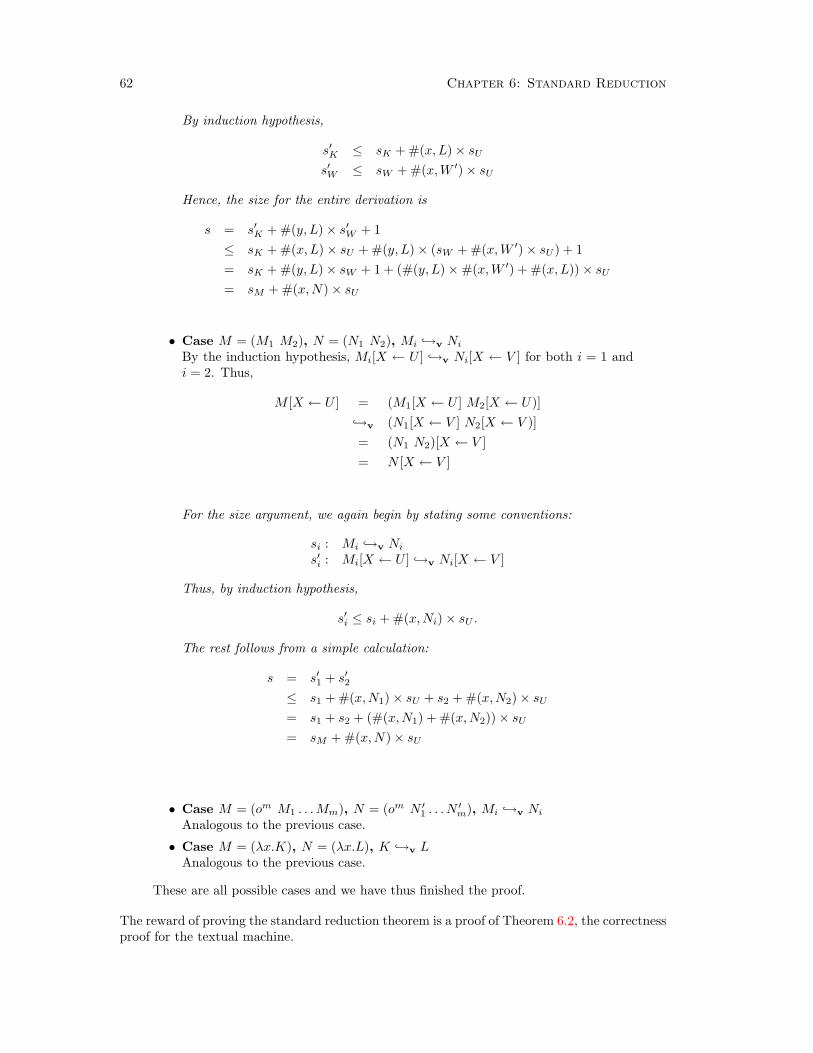
62 Chapter 6: Standard Reduction
By induction hypothesis,
s′K ≤ sK + #(x, L)× sU
s′W ≤ sW + #(x, W ′)× sU
Hence, the size for the entire derivation is
s = s′K + #(y, L)× s′W + 1≤ sK + #(x, L)× sU + #(y, L)× (sW + #(x,W ′)× sU ) + 1= sK + #(y, L)× sW + 1 + (#(y, L)×#(x,W ′) + #(x, L))× sU
= sM + #(x,N)× sU
• Case M = (M1 M2), N = (N1 N2), Mi →v Ni
By the induction hypothesis, Mi[X ← U ] →v Ni[X ← V ] for both i = 1 andi = 2. Thus,
M [X ← U ] = (M1[X ← U ] M2[X ← U)]→v (N1[X ← V ] N2[X ← V )]= (N1 N2)[X ← V ]= N [X ← V ]
For the size argument, we again begin by stating some conventions:
si : Mi →v Ni
s′i : Mi[X ← U ] →v Ni[X ← V ]
Thus, by induction hypothesis,
s′i ≤ si + #(x,Ni)× sU .
The rest follows from a simple calculation:
s = s′1 + s′2
≤ s1 + #(x,N1)× sU + s2 + #(x,N2)× sU
= s1 + s2 + (#(x, N1) + #(x,N2))× sU
= sM + #(x,N)× sU
• Case M = (om M1 . . .Mm), N = (om N ′1 . . . N ′
m), Mi →v Ni
Analogous to the previous case.
• Case M = (λx.K), N = (λx.L), K →v LAnalogous to the previous case.
These are all possible cases and we have thus finished the proof.
The reward of proving the standard reduction theorem is a proof of Theorem 6.2, the correctnessproof for the textual machine.
6.3 Observational Equivalence 63
Theorem 6.2: M→→v U if and only if M 7−→→v V for some value V and V →→v U .
In particular, if U ∈ b then M→→v U if and only if M 7−→→v U .
Proof for Theorem 6.2: To prove the left to right direction, assume that
M→→v U
and that M is not a value. It follows from Theorem 6.5 that there exists a standardreduction sequence L1 . . . Lp such that M = L1 and Lp = U . By induction on thelength of the sequence, there exists an index i such that Li is the first value in thesequence and
M = L1 7−→→v Li.
Set V = Li; trivially, Li→→v U . Moreover, constants can only be the end of a stan-dard reduction sequence of values if the standard reduction sequence is a singleton.Hence, the second part of the theorem concerning basic constants obviously holds.
In summary, we have shown that the specification of the evaluation function based on theequational system is equivalent to an evaluator based on the standard reduction function. Sincethe latter is a truly algorithmic specification, we can now implement the evaluator easily.
6.3 Observational Equivalence
Two expressions are of the same kind if both are values or both are applications (non-values).
Lemma 6.9 [Activity]: If M is a closed expression and evalv(C[M ]) exists, then
(i) either evalv(C[M ′]) exists for all closed expressions M ′ that are of the samekind as M ; or
(ii) for all closed expressions M ′ that are of the same kind as M , there is someevaluation context E such that
(a) if M is an application, then
C[M ′] 7−→→v E[M ′]
(b) if M is a λ-abstraction, then for some U ,
C[M ′] 7−→→v E[(M ′ U)]
(c) if M is a constant, then for some primitive on and basic constants b1, . . . bn,
C[M ′] 7−→→v E[(o b1 . . . M ′ . . . bn)]
Proof for Lemma 6.9: Intuitively, the proof proceeds by induction on the numberof standard reduction steps in the reduction:
C[M ] 7−→→v V
However, because M may be duplicated during βv-reductions, the induction hy-pothesis needs to be strengthened. The stronger claim is subject of the followinglemma.

64 Chapter 6: Standard Reduction
The formulation of an appropriate induction hypothesis for the Activity Lemma requires thenotion of a multi-hole context.
C = [ ]n| M| (λx.C)| (C C)| (on C . . . C)
A multi-hole context with m holes is well-formed if each hole [ ]i has a distinct label i ∈ [1,m].The notation C[M1, . . . Mn] means the expression generated by replacing each [ ]i in C with Mi.
The stronger version of Lemma 6.9 re-states the claim for m expressions and contexts withm holes.
Lemma 6.10: If M1, . . . Mm are closed expressions, C is a context with m holes,and evalv(C[M1, . . . Mm]) exists, then
(i) either evalv(C[M ′1, . . . M
′m]) for all closed expressions M ′
1, . . . M ′m that are of
the same kind as M1, . . . Mm, respectively; or
(ii) for all closed expressions M ′1, . . . M ′
m that are of the same kind as M1, . . . Mm,respectively, there is some evaluation context E such that for some i ∈ [1,m],
(a) if Mi is an application, then
C[M ′1, . . . M
′m] 7−→→v E[M ′
i ]
(b) if Mi is a λ-abstraction, then for some value U ,
C[M ′1, . . . M
′m] 7−→→v E[(M ′
i U)]
(c) if Mi is a constant, then for some primitive on and basic constants b1, . . . bn,
C[M ′1, . . . M
′m] 7−→→v E[(o b1 . . . M ′ . . . bm)]
Proof for Lemma 6.10: The proof is an induction on the number of standardreduction steps for the original program. If C[M1, . . . Mm] is a value, part (i) of theconclusion clearly applies. Consequently, assume that
C[M1, . . . Mm] 7−→v K 7−→→v V
for some expression K and value V . By Theorem 6.1, the program can be partitionedinto an evaluation context E′ and a redex (N L) such that
E′[(N L)] = C[M1, . . . Mm],
or into an evaluation context E′ and a redex (on b′1 . . . b′p) such that
E′[(on b′1 . . . b′p)] = C[M1, . . . Mm]
We deal with the first case; the proof of the second case proceeds in an analogousmanner.
1. Some expression Mi contains, or is equal to, the redex (N L). Since (N L)is an application and E′ an evaluation context, this is only possible if Mi isan application. If this is the case, the first clause of part (ii) of the lemma’sconclusion holds: for any expressions M ′
1, . . . M ′m of the correct kind,
E = C[M ′1, . . . M
′i−1, [ ]i, . . . M
′m]
6.3 Observational Equivalence 65
is an evaluation context. The key to this claim is that the expressions M ′1, . . .
M ′m are of the same kind as the expressions M1, . . . Mm, respectively. If
E′ = E1[(Mj E2)]
where Mj , 1 ≤ j ≤ m, is a value, and E1 and E2 are evaluation contexts, thenif M ′
j were an application, E would not be an evaluation context.
2. None of the expressions M1, . . . Mm contains the redex, but the redex containssome of these expressions. Now we must consider two subcases:
(a) Some λ-abstraction Mi is N . Now the second clause of part (ii) holds: forall closed expressions M ′
1, . . . M ′m,
E = C[M ′1, . . . M
′i−1, [ ]i, . . . M
′m]
and U differs from L only in occurrences of holes of C. Again, as in thepreceding case, E is an evaluation context because the expressions M ′
1, . . .M ′
m are of the right kind. Similarly, if L = Mj , for some j, 1 ≤ j ≤ m,then if M ′
j were not a value, U wouldn’t be a value.(b) The value N is a λ-abstraction, λX.N ′, that may contain some of the
expressions M1, . . . Mm. Now:
C[M1, . . . Mm] = E′[((λX.N ′) L)] 7−→v E′[N ′[L]← x]
As in the first subcase, since the expressions M ′1, . . . M ′
m are of the rightkind,
C[M ′1, . . . M
′m] = E′′[((λX.N ′′) L′)] 7−→v E′′[N ′′[L′]← x]
for some evaluation context E′′, expression N ′′, and value L′ that differaccordingly from E′, N ′, and L respectively. Since the expressions M1,. . . Mm are closed, there is some context C
′of q holes and a sequence of
indices 1 ≤ j1, . . . jq ≤ m such that
E′[N ′[L]← x] = C′[Mj1 , . . . Mjq
]
andE′′[N ′′[L′]← x] = C
′[M ′
j1 , . . . M′jq
]
The intermediate program satisfies the antecedent of our claim, the reduc-tion
C′[Mj1 , . . . ,Mjq
] 7−→→v V
is shorter, and therefore the induction hypothesis applies.
Equipped with the Activity Lemma, we are ready to finish Theorem 5.10 with the followinglemma. It shows the observational equivalence of two expressions that are not provably equal.
Lemma 6.11: Ω 'v (Ω (λx.x))
Proof for Lemma 6.11: Assume for some C that evalv(C[Ω]) exists. By theActivity Lemma, it could be the case that for all closed expressions M there is someevaluation context such that
C[M ] 7−→→v E[M ]

66 Chapter 6: Standard Reduction
But this contradicts the assumption that C[Ω] exists because E[Ω] is a divergingprogram. Hence, evalv(C[M ]) exists for all closed expressions M and in particularfor M = (Ω (λx.x)).
Conversely, assume that evalv(C[(Ω (λx.x))]) exists, then by an argument along thesame lines, evalv(C[Ω]) exists. Clearly, if one of the programs returns an abstraction,then so does the other, and both return the same basic constant. In short,
evalv(C[(Ω (λx.x))]) = evalv(C[Ω])
This proves that Ω 'v (Ω (λx.x)), because C is arbitrary.
6.4 Uniform Evaluation
Another question that can now be tackled is the following: what kind of behavior can weexpect from a machine given an arbitrary program? The evaluator can diverge for two differentreasons. First, every intermediate state of the evaluation may have a successor state. That is,the program is looping. Second, the evaluation may reach an intermediate state for which thestandard reduction function is undefined:
M1 7−→v M2 7−→v . . . 7−→v Mm
such that 7−→v is undefined for Mm and Mm is not an answer. For this to be the case, Mm
must contain an application consisting of values in the hole of an evaluation contexts such thatneither the βv nor the δ reduction applies, i.e.,
Mm = E[(U V )] where U is not a basic constantor
Mm = E[(on V1 . . . Vn)] where some Vi is a λ-abstractionor δ(on, V1, . . . , Vn)is undefined
Adopting a machine-oriented view, programs for which 7−→v is undefined are called stuckstates. Stuck states play an important role in the analysis of machines and other programminglanguage tools. A precise understanding of the stuck states of any given programming languageis therefore crucial. We first give a formal definition of ISWIM stuck states.
An application M is stuck if
1. M = (om b1 . . . bm) and δ(om, b1, . . . bm) is undefined; or
2. M = (om b1 . . . bi−1 (λX.N) bi+1 . . . bm); or
3. M = (b V ).
A program M is stuck if M = E[N ] for some evaluation context E and a stuck applicationN .
A program in pure ISWIM can only evaluate to a value, a stuck program, or diverge.
Lemma 6.12: If M is a closed expression, then either
1. M 7−→→v V for some value V ;
2. M 7−→→v N for some stuck program N ;
3. for all N such that M 7−→→v N , there exists an L such that N 7−→v L.

6.4 Uniform Evaluation 67
Proof for Lemma 6.12: Assume there exists an N such that M 7−→→v N and7−→v is undefined for N . That is,
M1 7−→v M2 7−→v M3 7−→v . . . 7−→v Mm = N
By Unique Evaluation (Lemma 6.1), N is either a value, or there is an evaluationcontext E, possibly a primitive on, and values U , V , V1, . . . Vn such that
N = E[(U V )] or N = E[(on V1 . . . Vn)]
If the applications in the hole are redexes, we have a contradiction to our assumption.Consequently, U is neither a λ-abstraction nor a primitive but is a basic constant.Similarly, some Vi must not be a basic constant or δ(on, V1, . . . Vn) is not defined.Hence, N is a stuck program. In conclusion, programs either diverge, or reduce toa value or to a stuck state.
Chapter 10 defines a language with a uniform treatment of stuck states.

68 Chapter 6: Standard Reduction

69
Chapter 7: Machines
Every evaluation cycle in the standard-reduction textual machine performs three steps:
1. It tests whether the program is a value; if so, the machine stops.
2. If the program is an application, the machine partitions the program into an evaluationcontext, E, and an application, (U V ) or (on V1 . . . Vn).
3. If the application is a βv or δ redex, the machine constructs the contractum M and fillsthe evalutaion context E with the contractum M .
The result of such a step is the program E[M ], which is the next machine state. Now theevaluation cycle starts over.
An obvious inefficiency in this machine is the repeated partitioning of a program into anevaluation context and a redex. Clearly, the evaluation context of the (n + 1)st step is oftenthe same as, or at least, is closely related to the one for the nth step. For example, considerthe evaluation of
(add1 ((λx.((λy.((λz.x) d3e)) d2e)) d1e))
which is a fairly typical example:
(add1 ((λx.((λy.((λz.x) d3e)) d2e)) d1e))
7−→v (add1 ((λy.((λz.d1e) d3e)) d2e))
7−→v (add1 ((λz.d1e) d3e))
7−→v (add1 d1e)
7−→vd2e.
The redexes in each intermediate state are underlined, the evaluation context is the part of theterm that is not underlined. The evaluation context for the first three states is (add1 [ ]). Butthe machine has to recompute the evaluation context at every stage.
Depending on the use of the standard-reduction machine, the efficiency may not be an issue.For example, if the goal of the machine is simply to formally define evalsv, then efficiency is ofno interest. However, if we want to explain an implementation of a language to others, thenwe may want to formalize a more “realistic” definition of the language. In particular, no realimplementation of an ISWIM-like language would find the context from scratch on each step.
7.1 CC Machine
To eliminate repeated context computations, we can separate program states into the “currentsubterm of interest” and the “current evaluation context.” Putting the former into the hole ofthe latter yields the complete program. We will refer to the term of interest as the controlstring M and the evaluation context simply as the context E. These two elements are pairedtogether to form the machine’s state: 〈M,E〉. The machine is called the CC machine.
In addition to the reduction tasks of the textual machine, the CC machine is responsible forfinding the redex. Initially, the entire program is the control string, and the initial evaluationcontext is the empty context. The machine’s search instructions implement rules 1 and 2′ fromthe beginning of the previous chapter. That is, if the control string is not an application thatconsists of values, the leftmost non-value becomes the control string, and the rest becomes apart of the evaluation context.
For example, if the control string is ((K L) N) and the evaluation context is E, then themachine must search for the redex in (K L), and it must remember the shape of the rest of the

70 Chapter 7: Machines
program. Consequently the next state of the machine must have (K L) as the control stringcomponent and must refine the current context E to a context of the shape E[([ ] N)]. In otherwords, the CC machine must have a state transition of the form
〈(M N), E〉 7−→v 〈M,E[([ ] N)]〉 if M 6∈ V
Search rules for other shapes of applications are needed, too.After the control string becomes a redex, the CC machine must simulate the actions of the
textual machine on a redex. Thus it must have the following two instructions:
〈(om b1 . . . bm), E〉 7−→v 〈V,E〉 where V = δ(om, b1, . . . , bm) [ccδ]
〈((λX.M)V ), E〉 7−→v 〈M [X ← V ], E〉 [ccβv]
The result of such a transition can be a state that pairs a value with an evaluation contexts.In the textual machine, this corresponds to a step of the form E[L] 7−→v E[V ]. The textualmachine would actually divide E[V ] into a new redex L′ and a new evaluation context E′
that is distinct from E. But the textual machine clearly does not pick random pieces fromthe evaluation context to form the next redex. If E = E∗[((λX.M) [ ])], then E′ = E∗ andL′ = ((λX.M) V ). That is, the new redex is formed of the innermost application in E, and E′
is the rest of E.Thus, for a faithful simulation of the textual machine, the CC machine needs a set of
instructions that exploit the information surrounding the hole of the context when the controlstring is a value. In the running example, the CC machine would have to make a transitionfrom
〈V,E∗[((λX.M) [ ])]〉
to〈((λX.M) V ), E∗〉
At this point, the control string is an application again, and the search process can start over.Putting it all together, the evaluation process on a CC machine consists of shifting pieces
of the control string into the evaluation context such that the control string becomes a redex.Once the control string has turned into a redex, an ordinary contraction occurs. If the result isa value, the machine must shift pieces of the evaluation context back to the control string.
The 7−→cc reduction relation on CC machine states is defined as follows:
〈(M N), E〉 7−→cc 〈M,E[([ ] N)]〉 [cc1]
if M 6∈ V〈(V1 M), E〉 7−→cc 〈M,E[(V1 [ ])]〉 [cc2]
if M 6∈ V〈(on V1 . . . Vi M N . . .), E〉 7−→cc 〈M,E[(on V1 . . . Vi [ ] N . . .)]〉 [cc3]
if M 6∈ V〈((λX.M) V ), E〉 7−→cc 〈M [X ← V ], E〉 [ccβv]
〈(om b1 . . . bm), E〉 7−→cc 〈V,E〉 [ccδ]
where V = δ(om, b1, . . . bm)〈V,E[(U [ ])]〉 7−→cc 〈(U V ), E〉 [cc4]
〈V,E[([ ] N)]〉 7−→cc 〈(V N), E〉 [cc5]
〈V,E[(on V1 . . . Vi [ ] N . . .)]〉 7−→cc 〈(on V1 . . . Vi V N . . .), E〉 [cc6]
evalcc(M) =
b if 〈M, [ ]〉 7−→→cc 〈b, [ ]〉function if 〈M, [ ]〉 7−→→cc 〈λX.N, [ ]〉
By the derivation of the CC machine, it is almost obvious that it faithfully implements thetextual machine. Since evaluation on both machines is defined as a partial function from

7.1 CC Machine 71
programs to answers, a formal justification for this claim must show that the two functions areidentical.
Theorem 7.1: evalcc = evalsv.
Proof for Theorem 7.1: We need to show that if evalcc(M) = A then evalsv(M) =A and vice versa. By the definition of the two evaluation functions, this requires aproof that
M 7−→→v V if and only if 〈M, [ ]〉 7−→→cc 〈V, [ ]〉.A natural approach to the proof of this claim is an induction of the length of the giventransition sequence. However, since intermediate states have non-empty evaluationcontexts, we will need a slightly stronger induction hypothesis:
E[M ] 7−→→v V if and only if 〈M,E〉 7−→→cc 〈V, [ ]〉.
The hypothesis clearly implies the general theorem. Thus the rest of the proof isa proof of this intermediate claim. The proof for each direction is an induction onthe length of the reduction sequence.
To prove the left-to-right direction of the claim, assume E[M ] 7−→→v V . If the re-duction sequence is empty, the conclusion is immediate, so assume there is at leastone step:
E[M ] 7−→v E′[N ] 7−→→v V
where LvN for some application expression L where E′[L] = E[M ]. By the induc-tive hypothesis, 〈N,E′〉 7−→→cc 〈V, [ ]〉. To conclude the proof, we must show that
〈M,E〉 7−→→cc 〈N,E′〉
If L is inside M (or the same), then E′ must be an extension of E (or the same).Otherwise, M must be a value, because it is inside the redex and also in an evalautionposition. Thus, depending on the shape of M and E, there are four possibilities:
• Case M = E′′[L]Then, E′ = E[E′′]. By Lemma 7.2 below, 〈M,E〉 7−→→cc 〈L,E[E′′]〉 and, hence,by a [ccδ] or [ccβv] transition, 〈L, E[E′′]〉 7−→→cc 〈N,E[E′′]〉.• Case E = E′[((λX.N ′) [ ])],M ∈ V
A first step puts the redex into the control position, which enables a [ccβv]
reduction:
〈M,E′[((λX.N ′) [ ])]〉 7−→cc 〈((λX.N ′) M), E′〉7−→cc 〈N ′[X ←M ], E′〉
Since the assumptions imply that N = N ′[X ←M ], this proves the conclusion.• Case E = E′′[([ ] K)],M ∈ V
Depending on the nature of K, there are two different scenarios:1. If K ∈ V then L = (M K), which implies the conclusion.2. If K 6∈ V then there exists an evaluation context E′′′ such that K = E′′′[L].
Hence, E′ = E′′[(M E′′′[L])] and
〈M,E′′[([ ] K)]〉 7−→cc 〈(M K), E′′〉7−→cc 〈K, E′′[(M [ ])]〉7−→→cc 〈L,E′′[(M E′′′)]〉 by Lemma 7.27−→→cc 〈N,E′′[(M E′′′)]〉
= 〈N,E′〉.

72 Chapter 7: Machines
• Case E = E′[(on b1 . . . [ ] . . . bn)],M ∈ bAppropriate adaptations of the proofs of the second and third case prove theconclusion.
For the right-to-left direction, assume 〈M,E〉 7−→→cc 〈V, [ ]〉. The proof is a again aninduction on the number of transition steps. If there are none, M ∈ V and E = [ ],which implies the claim. Otherwise, there is a first transition step:
〈M,E〉 7−→cc 〈N,E′〉 7−→→cc 〈V, [ ]〉
By inductive hypothesis, E′[N ] 7−→→v V . The rest of the proof depends on whichkind of transition the CC machine made to reach the state 〈N,E′〉. If the first tran-sition was one of [cc1], . . . [cc6], then E[M ] = E′[N ], and the conclusion follows. If itis a [ccβv] or a [ccδ] transition, then E[M ] 7−→v E′[N ], so E[M ] 7−→v E′[N ] 7−→→v V .
Lemma 7.2: If M = E′[L] and Lv L′ for some L′, then
〈M,E〉 7−→→cc 〈L,E[E′]〉
Proof for Theorem 7.2: The proof is an induction on the structure of E′. IfE′ = [ ] then the conclusion is immediate. Otherwise, E′ has one of the followingthree shapes:
E′ = (E′′ N)E′ = (V E′′)E′ = (om V1 . . . Vn E′′ N . . .)
In each case, the machine can move the pieces surrounding E′′ to the context com-ponent, e.g.,
〈(E′′[L] N), E〉 7−→cc 〈E′′[L], E[([ ] N)]〉
Since E′′ is a component of E′, the conclusion follows from the inductive hypothesis.
Exercise 7.1. Show the reduction of
〈 ( ((λf.λx.f x) λy.(+ y y)) d1e) , [ ]〉
to 〈V, [ ]〉 with 7−→cc.
Exercise 7.2. Implement the CC machine in your favorite programming language.
7.2 SCC Machine
The CC machine faithfully immitates the textual machine by performing all of the work on thecontrol string. Consider the following example:
((λx.x) ((λx.x) d5e)),
consisting of an application of two applications, which evaluates as follows:
〈((λx.x) ((λx.x) d5e)), [ ]〉 7−→cc 〈((λx.x) d5e), ((λx.x) [ ])〉7−→cc 〈d5e, ((λx.x) [ ])〉

7.2 SCC Machine 73
At this point, the CC machine is forced to construct an application such that one of theapplication rules can put the second application in the control string register:
. . . 7−→cc 〈((λx.x) d5e), [ ]〉7−→cc 〈d5e, [ ]〉.
The next to last step is only needed because the CC machine only exploits information in thecontrol string position. One way to simplify the CC machine is to combine the rules for valueswith the reduction of redexes such that the last two steps become one step.
A similar simplification is possible when the value returned belongs into the function posi-tion. A simple variation of the first example shows how the machine again moves informationinto the control string even though the next step is clear:
〈(((λx.x) (λx.x)) ((λx.x) d5e)), [ ]〉 7−→cc 〈((λx.x) (λx.x)), ([ ] ((λx.x) d5e))〉7−→cc 〈(λx.x), ([ ] ((λx.x) d5e))〉.
Now the machine constructs an application only to move on to the evaluation of the argumentexpression:
7−→cc 〈((λx.x) ((λx.x) d5e)), [ ]〉7−→cc 〈((λx.x) d5e), ((λx.x) [ ])〉. . .
Instead of constructing the application, the machine could always put the argument into thecontrol register and put the value for the function position into the evaluation context. If theargument is a value, the modified machine can perform a reduction. If not, the current CCmachine would have reached this state, too.
Once we have a machine that combines the recognition of a value with the reduction of aredex, when possible, we can also omit the specialized treatment of applications. The current CCmachine has three distinct transitions for dealing with applications and three more for dealingwith primitive applications. Side-conditions ensure that only one transition applies to any givenapplication. These separate rules are only necessary because the machine performs all the workon the control string and uses the control stack only as a simple memory. Together with theperviously suggested simplifications, we can eliminate the side-conditions, the reduction rules,and the rule [cc2], which only exists to move arguments from evaluation contexts into the controlstring position.
The simplified CC machine has fewer transitions and no side-conditions. Given a statefinding the applicable transition rule is easy. If the control string is an application, shift afixed portion to the evaluation context and concentrate on one sub-expression. If it is a value,check the innermost application of the evaluation context. If the hole is in the last positionof the application, perform a reduction, otherwise swap information between the control stringregister and the evaluation context register.
〈(M N), E〉 7−→scc 〈M,E[([ ] N)]〉 [scc1]
〈(on M N . . .), E〉 7−→scc 〈M,E[(on [ ] N . . .)]〉 [scc2]
〈V,E[((λX.M) [ ])]〉 7−→scc 〈M [X ← V ], E〉 [scc3]
〈V,E[([ ] N)]〉 7−→scc 〈N,E[(V [ ])]〉 [scc4]
〈b, E[(on b1 . . . bi [ ])]〉 7−→scc 〈V,E〉 [scc5]
where δ(on, b1, . . . , bi, b) = V〈V,E[(on V1 . . . Vi [ ] N L . . .)]〉 7−→scc 〈N,E[(on V1 . . . Vi V [ ] L . . .)]〉 [scc6]
evalscc(M) =
b if 〈M, [ ]〉 7−→→scc 〈b, [ ]〉function if 〈M, [ ]〉 7−→→scc 〈λX.N, [ ]〉

74 Chapter 7: Machines
The CC machine and the simplified version define the same evaluation function.
Theorem 7.3: evalscc = evalcc.
Proof for Theorem 7.3: The proof of this theorem is analoguous to the proof ofTheorem 7.1. That is, unfolding the definition of the two evaluation functions leadsto the proof obligation that
〈M, [ ]〉 7−→→cc 〈V, [ ]〉 if and only if 〈M, [ ]〉 7−→→scc 〈V, [ ]〉.
The correct stregthening of this claim to an inductive hypothesis extends it toarbitrary intermediate states:
〈M,E〉 7−→→cc 〈V, [ ]〉 if and only if 〈M,E〉 7−→→scc 〈V, [ ]〉.
The key idea for the proof of the intermediate claim is that for any given program,the CC machine and the SCC machine quickly synchronize at some state providedthe initial state leads to a result. More precisely, given 〈M,E〉 such that E[M ] =E′[L] and L is a v-redex, there exists a state 〈N,E′′〉 such that
〈M,E〉 7−→+cc 〈N,E′′〉 and 〈M,E〉 7−→+
scc 〈N,E′′〉
By definition, M is either a value or an expression that contains a redex. Moreover,if M is a value, the evaluation context must contain an innermost application:E = E′[(o V1 . . . Vm [ ] N1 . . . Nn)], E = E′[(V [ ])], or E = E′[([ ] N)]. Hence, theinitial state 〈M,E〉 falls into one of the following four possibilities:
• Case M = E′[L]The CC machine evaluates the initial state as follows:
〈E′[L], E〉 7−→→cc 〈L,E[E′]〉 7−→cc 〈N,E[E′]〉
The SCC machine eventually reaches the same state, but the intermediatestates depend on the shape of the redex L. If L = ((λX.L′) L′′), then the SCCmachine reaches 〈L′′, E[E′[((λX.L′) [ ])]]〉 as the next to last state; otherwise,the next to last state is 〈b, E[E′[(on b1 . . . bi [ ])]]〉 where L = (on b1 . . . bi b).
• Case M ∈ V,E = E′[((λX.L′) [ ])]In this case, the CC machine creates a redex in the control component andreduces it:
〈M,E′[((λX.L′) [ ])]〉 7−→cc 〈((λX.L′) M), E′〉7−→cc 〈L′[X ←M ], E′〉
The SCC machine avoids the first step and immediately goes into the samestate.
• Case M ∈ V,E = E′[([ ] N)]If N ∈ V , the proof of this case proceeds along the lines of the second case.Otherwise,
〈M,E′[([ ] N)]〉 7−→cc 〈(M N), E′〉, 7−→cc 〈N,E′[(M [ ])]〉
Again, the SCC machine skips the intermediate state.
• Case M ∈ V,E = E′[(op V1 . . . Vm [ ] N1 . . . Nn)]The transition sequences depend on the shape of the sequence N1, . . . Nn.There are three possible cases:

7.3 CK Machine 75
1. If the sequence N1, . . . Nn is empty, M , V1, . . . Vm must be basic constantsand δ(op, V1, . . . Vm, V ) = U for some value U . It follows that
〈M,E′[(op V1 . . . Vn [ ])]〉 7−→cc 〈(op V1 . . . Vn M), E′〉7−→cc 〈U,E′〉
As in the previous case, the SCC machine reaches the final state by skipingthe intermediate state.
2. If N1, . . . Nn is not empty but N1, . . . Nn ∈ V , then
〈M,E′[(op V1 . . . Vm [ ] N1 . . . Nn)]〉7−→cc 〈(op V1 . . . Vm M N1 . . . Nn), E′〉7−→cc 〈U,E′〉.
Now, the SCC machine needs to perform a number of additional steps,which serve to verify that the additional arguments are values:
〈M,E′[(op V1 . . . Vm [ ] N1 . . . Nn)]〉7−→scc 〈N1, E
′[(o V1 . . . Vm M [ ] N2 . . . Nn)]〉7−→→scc . . .7−→→scc 〈Nn, E′[(op V1 . . . Nn−1 [ ])]〉7−→scc 〈U,E′〉.
3. If N1, . . . Nn is not empty and Ni 6∈ V , then both machines reach theintermediate state
〈Ni, E′[(op V1 . . . VnN1 . . . Ni−1 [ ] Ni+1 . . .)]〉
after an appropriate number of steps.
The rest of the proof is a straightforward induction on the number of transitionsteps. Assume 〈M,E〉 7−→→cc 〈V, [ ]〉. If M = V,E = [ ], the conclusion is immediate.Otherwise, E[M ] must contain a redex since the machine reaches a final state. Bythe above, there must be an intermediate state 〈N,E′〉 that both machines reachafter some number of steps. By the inductive hypothesis, both machines also reach〈V, [ ]〉 from this intermediate state. The proof of the opposite direction proceeds inthe same fashion.
Exercise 7.3. Show the reduction of
〈 ( ((λf.λx.f x) λy.(+ y y)) d1e) , [ ]〉
to 〈V, [ ]〉 with 7−→scc.
Exercise 7.4. Implement the SCC machine.
7.3 CK Machine
Each step of an evaluation on the CC or simplified CC machine refers to the innermost appli-cation of the evaluation context—that is, the application that directly contains the hole. Inthe case that the control string is an application, a new innermost application is created in thecontext. In the case that the control string turns into a value, the next step is determined byconsidering the innermost application. In short, the transitions always access the evaluation

76 Chapter 7: Machines
context from the inside and in a last-in, first-out fashion. Transition steps depend on the preciseshape of the first element but not on the rest of the data structure.
The observation suggests that the evaluation context register should be a list of applicationswith a hole, so that the innermost part is easily accessed or added at the front of the list:
κ = κs . . .κs = (V [ ])
| ([ ] N)| (on V . . . V [ ] N . . .)
For readability and for ease of implementation, we tag each case of this construction and invertthe list of values in a primitive application:
κ = mt| 〈fun, V, κ〉| 〈arg, N, κ〉| 〈opd, 〈V, . . . , V, on〉, 〈N, . . .〉, κ〉
This data structure is called a continuation. The 7−→ck relation maps an expression–continuationpair to a new expression–continuation pair.
〈(M N), κ〉 7−→ck 〈M, 〈arg, N, κ〉〉 [ck1]
〈(on M N . . .), κ〉 7−→ck 〈M, 〈opd, 〈on〉, 〈N, . . .〉, κ〉〉 [ck2]
〈V, 〈fun, (λX.M), κ〉〉 7−→ck 〈M [X ← V ], κ〉 [ck3]
〈V, 〈arg, N, κ〉〉 7−→ck 〈N, 〈fun, V, κ〉〉 [ck4]
〈b, 〈opd, 〈bi, . . . b1, on〉, 〈〉, κ〉〉 7−→ck 〈V, κ〉 [ck5]
where δ(on, b1, . . . , bi, b) = V〈V, 〈opd, 〈V ′, . . . on〉, 〈N,L, . . .〉, κ〉〉 7−→ck 〈N, 〈opd, 〈V, V ′, . . . on〉, 〈L, . . .〉, κ〉〉 [ck6]
evalck(M) =
b if 〈M, mt〉 7−→→ck 〈b, mt〉function if 〈M, mt〉 7−→→ck 〈λX.N, mt〉
Given an SCC state, we can find a corresponding CK state and vice versa, based on a bijectionbetween the set of evaluation contexts and the set of continuation codes:
Tck→scc(κ) =
[ ] if κ = mtE′[([ ] N)] if κ = 〈arg, N, κ′〉E′[(V [ ])] if κ = 〈fun, V, κ′〉E′[(on V1 . . . Vi [ ] N . . .)] if κ = 〈opd, 〈Vi, . . . V1, o
n〉, 〈N, . . .〉, κ′〉where E′ = Tck→scc(κ′)
Tscc→ck(E) =
mt if E = [ ]〈arg, N, κ′〉 if E = E′[([ ] N)]〈fun, V, κ′〉 if E = E′[(V [ ])]〈opd, 〈Vi, . . . , V1, o
n〉, 〈N, . . .〉, κ′〉 if E = E′[(on V1 . . . Vi [ ] N . . .)]where κ′ = Tscc→ck(E′)
Based on this bijection between CC and CK states, it is easy to prove the correctness of theevaluation function based on the CK machine.
Theorem 7.4: evalck = evalscc.
Proof for Theorem 7.4: Based on the translations between states, we can checkthat

7.4 CEK Machine 77
1. if 〈M,E〉 7−→scc 〈N,E′〉, then 〈M, Tscc→ck(E)〉 7−→ck 〈N, Tscc→ck(E′)〉;
2. if 〈M,κ〉 7−→ck 〈N,κ′〉, then 〈M, Tck→scc(κ)〉 7−→scc 〈N, Tck→scc(κ′)〉.
By trivial inductions on the length of the transition sequences, it follows that
〈M, [ ]〉 7−→→scc 〈V, [ ]〉 if and only if 〈M, mt〉 7−→→ck 〈V, mt〉,
which implies the theorem.
Exercise 7.5. Show the reduction of
〈 ( ((λf.λx.f x) λy.(+ y y)) d1e) , mt〉
to 〈V, mt〉 with 7−→ck.
Exercise 7.6. Implement the CK machine.
7.4 CEK Machine
For all of the machines so far, the reduction of a βv-redex requires the substitution of a valuein place of all occurrences of an identifier. A naive implementation of this substituion would beexpensive, especially as expressions become large. Furthermore, in the case that substitutionprocedures a non-value expression, the machine will imemdiately re-visit sub-expressions (toevaluate them) that were just visited by substituion.
Unlike the simplication we found for evaluation contexts, we cannot avoid substitutiontraversals and re-traversals by turning the expression inside-out. We can, however, delay thework of substituion until it is actually needed.
To represent delayed substitutions, every expression in the machine is replaced by a pairwhose first component is an open term and whose second component is a function that maps allfree variables to their correponding expressions. The pair is called a closure, and the functioncomponent is an environment.
Of course, environments cannot map variables to expressions, because this would re-introduceexpressions into the machine; it must map variables to closures. Thus, environments E and clo-sures c and v have mututally recursive definitions:
E = a function 〈X, c〉, . . .c = 〈M, E〉 | FV(M) ⊂ dom(E)v = 〈V, E〉 | 〈V, E〉 ∈ c
E [X ← c] = 〈X, c〉 ∪ 〈Y, c′〉 | 〈Y, c′〉 ∈ E and Y 6= X
Based these defininitions, we can reformulate the CK machine into a machine that works oncontrol strings with environments and continuation codes: the CEK machine. Continuationsin this machine contain closures instead of expressions.
κ = mt| 〈fun, v, κ〉| 〈arg, c, κ〉| 〈opd, 〈v, . . . , v, on〉, 〈c, . . .〉, κ〉

78 Chapter 7: Machines
The transitions are similar to CK transitions, except the expressions are replaced with closures,and substitution is replaced by environment update.
〈〈(M N), E〉, κ〉 7−→cek 〈〈M, E〉, 〈arg, 〈N, E〉, κ〉〉 [cek1]
〈〈(on M N . . .), E〉, κ〉 7−→cek 〈〈M, E〉, 〈opd, 〈on〉, 〈〈N, E〉, . . .〉, κ〉〉 [cek2]
〈〈V, E〉, 〈fun, 〈(λX1.M), E ′〉, κ〉〉 7−→cek 〈〈M, E ′[X1 ← 〈V, E〉]〉, κ〉 [cek3]
if V 6∈ X〈〈V, E〉, 〈arg, 〈N, E ′〉, κ〉〉 7−→cek 〈〈N, E ′〉, 〈fun, 〈V, E〉, κ〉〉 [cek4]
if V 6∈ X〈〈b, E〉,〈opd, 〈〈bi, Ei〉, . . . 〈b1, E1〉, on〉, 〈〉, κ〉〉
7−→cek 〈〈V, ∅〉, κ〉 [cek5]
where δ(on, b1, . . . , bi, b) = V〈〈V, E〉,〈opd, 〈v′, . . . on〉, 〈〈N, E ′〉, c, . . .〉, κ〉〉
7−→cek 〈〈N, E ′〉,〈opd, 〈〈V, E〉, v′, . . . on〉, 〈c, . . .〉, κ〉〉
[cek6]
if V 6∈ X〈〈X, E〉, κ〉 7−→cek 〈c, κ〉 [cek7]
where E(X) = c
evalcek(M) =
b if 〈〈M, ∅〉, mt〉 7−→→cek 〈〈b, E〉, mt〉function if 〈〈M, ∅〉, mt〉 7−→→cek 〈〈λX.N, E〉, mt〉
Given a CEK state, we can find a corresponding CK state with an “unload” function thatreplaces every closure in the state by the closed term that it represents:
U(〈M, 〈X1, c1〉, . . . 〈Xn, cn〉〉) = M [X1 ← U(c1)] . . . [Xn ← U(cn)]
Since closures also occur inside of CEK continuation codes, the translation of CEK states intoCK states requires an additional traversal of CEK continuation codes to replace these closures:
Tcek→ck(κ) =
[ ] if κ = mt〈arg,U(c), κ∗〉 if κ = 〈arg, c, κ′〉〈fun,U(c), κ∗〉 if κ = 〈fun, c, κ′〉〈opd, 〈U(c′), . . . on〉, 〈U(c), . . .〉, κ∗〉
if κ = 〈opd, 〈c′, . . . on〉, 〈c, . . .〉, κ′〉where κ∗ = Tcek→ck(κ′)
Unfortunately, it is impossible to define inverses of the U and Tcek→ck functions; given a closedterm, there are many closures that map back to the same term. As a result, the simpleproof method of the preceding adequacy theorems for verifying the equality between the SCCevaluator and the CK evaluator fails here. However, as in the preceding sections, it is still thecase that the CEK machine can simulate any given sequence of CK states if the initial state ofthe two machines are equivalent.
Theorem 7.5: evalcek = evalck.
Proof for Theorem 7.5: Given the translation from CEK states, we can checkthat for any intermediate state 〈c, κ〉 in the sequence of CEK states, there is a state〈c′, κ′〉 such that
〈c, κ〉 7−→→cek 〈c′, κ′〉
and〈U(c), Tcek→ck(κ)〉 7−→ck 〈U(c′, Tcek→ck(κ′))〉
Hence, 〈〈M, ∅〉, mt〉 7−→→cek 〈〈V, E〉, mt〉 implies 〈M, mt〉 7−→ck 〈U(〈V, E〉), mt〉, whichproves the left-to-right direction.
7.4 CEK Machine 79
The right-to-left direction requires a stronger induction hypothesis than the left-to-right direction or the inductions of the preceding adequacy theorems because of thelack of a function from CK states to CEK states. In addition to the intial state ofthe transition sequence of the CK machine, we need to know the initial state of theCEK machine:
For every CK state 〈M1, κ1〉 and CEK state 〈〈M ′1, E〉, κ′1〉 such that M1 =
U(〈M ′1, E〉) and κ1 = Tcek→ck(κ′1), if
〈M1, κ1〉 7−→→ck 〈V, mt〉
then for some closure cl with U(c) = V ,
〈〈M ′1, E〉, κ′1〉 7−→→cek 〈c, mt〉
The theorem follows from specializing the two initial states to 〈M, mt〉 and 〈〈M, ∅〉, mt〉.The proof of the claim is by induction on the length of the transition sequence inthe CK machine. It proceeds by case analysis of the initial state of the CK machine:
• Case M1 = (L N)The CK machine performs a [ck1] instruction:
〈(L N), κ1〉 7−→ck 〈L, 〈arg, N, κ1〉〉
By assumption, 〈M ′1, E〉 = 〈(L′ N ′), E〉 such that L = U(〈L′, E〉) and N =
U(〈N ′, E〉) since U preserves the shape of applications in the translation pro-cess. Hence,
〈〈(L′ N ′), E〉, κ′1〉 7−→ck 〈〈L′, E〉, 〈arg, 〈N ′, E〉, κ′1〉〉.
Clearly, Tcek→ck(〈arg, 〈N ′, E〉, κ′1〉) = 〈arg, N, κ1〉. Thus the inductive hypoth-esis applies and proves the claim for this case.
• Case M1 ∈ V, κ1 = 〈fun, (λX.N), κ2〉Here the CK transition sequence begins as follows:
〈M1, 〈fun, (λX.N), κ2〉〉 7−→ck 〈N [X ←M1], κ2〉
Given the definition of U , there are two kinds of CEK states that can map tothe given CK state:
– Case M ′1 6∈ X
In this case, the CEK step directly corresponds to the CK step:
〈〈M ′1, E〉, 〈fun, 〈(λX.N), E ′〉, κ2〉〉7−→cek 〈〈N, E ′[X ← 〈M ′
1, E〉]〉, κ2〉
– Case M ′1 ∈ X, U(E(M ′
1)) = M1
If the value is a variable, the CEK machine first looks up the value of thevariable in the environment before it performs an appropriate transition:
〈〈M ′1, E〉, 〈fun, 〈(λX.N ′), E ′〉, κ2〉〉7−→cek 〈E(M ′
1), 〈fun, 〈(λX.N), E ′〉, κ2〉〉7−→cek 〈〈N, E ′[X ← E(M ′
1)]〉, κ2〉

80 Chapter 7: Machines
In both cases, the assumptions state U(〈M ′1, E〉) = M1. Hence, to finish the
case, we must show that
U(〈N ′, E ′[X ← c]〉) = N [X ← U(c)]
where cl = 〈M ′1, E〉. From the definition of U , if E = 〈X1, c1〉, . . . , 〈X1, c1〉,
U(〈λX.N ′, E ′〉) = λX.N ′[X1 ← U(c1)] . . . [Xn ← U(cn)] = λX.N,
which impliesN ′[X1 ← U(c1)] . . . [Xn ← U(cn)] = N.
By the Substitution Lemma,
N [X ← U(c)] = N ′[X1 ← U(c1)] . . . [Xn ← U(cn)][X ← U(c)]= U(〈N ′, E [X ← c]〉).
The rest follows again by induction on the length of the CK transition sequence.
The proof of the other cases are analoguous to the last one.
Exercise 7.7. Show the reduction of
〈〈 ( ((λf.λx.f x) λy.(+ y y)) d1e) , ∅〉, mt〉
to 〈〈V, E〉, mt〉 with 7−→cek.
Exercise 7.8. Implement the CEK machine.

7.4 CEK Machine 81
7.5 Machine Summary
CC machine
〈(M N), E〉 7−→cc 〈M,E[([ ] N)]〉 [cc1]
if M 6∈ V〈(V1 M), E〉 7−→cc 〈M,E[(V1 [ ])]〉 [cc2]
if M 6∈ V〈(on V1 . . . Vi M N . . .), E〉 7−→cc 〈M,E[(on V1 . . . Vi [ ] N . . .)]〉 [cc3]
if M 6∈ V〈((λX.M) V ), E〉 7−→cc 〈M [X ← V ], E〉 [ccβv]
〈(om b1 . . . bm), E〉 7−→cc 〈V,E〉 [ccδ]
where V = δ(om, b1, . . . bm)〈V,E[(U [ ])]〉 7−→cc 〈(U V ), E〉 [cc4]
〈V,E[([ ] N)]〉 7−→cc 〈(V N), E〉 [cc5]
〈V,E[(on V1 . . . Vi [ ] N . . .)]〉 7−→cc 〈(on V1 . . . Vi V N . . .), E〉 [cc6]
evalcc(M) =
b if 〈M, [ ]〉 7−→→cc 〈b, [ ]〉function if 〈M, [ ]〉 7−→→cc 〈λX.N, [ ]〉
SCC machine
〈(M N), E〉 7−→scc 〈M,E[([ ] N)]〉 [scc1]
〈(on M N . . .), E〉 7−→scc 〈M,E[(on [ ] N . . .)]〉 [scc2]
〈V,E[((λX.M) [ ])]〉 7−→scc 〈M [X ← V ], E〉 [scc3]
〈V,E[([ ] N)]〉 7−→scc 〈N,E[(V [ ])]〉 [scc4]
〈b, E[(on b1 . . . bi [ ])]〉 7−→scc 〈V,E〉 [scc5]
where δ(on, b1, . . . , bi, b) = V〈V,E[(on V1 . . . Vi [ ] N L . . .)]〉 7−→scc 〈N,E[(on V1 . . . Vi V [ ] L . . .)]〉 [scc6]
evalscc(M) =
b if 〈M, [ ]〉 7−→→scc 〈b, [ ]〉function if 〈M, [ ]〉 7−→→scc 〈λX.N, [ ]〉
CK machine
κ = mt| 〈fun, V, κ〉| 〈arg, N, κ〉| 〈opd, 〈V, . . . , V, on〉, 〈N, . . .〉, κ〉
〈(M N), κ〉 7−→ck 〈M, 〈arg, N, κ〉〉 [ck1]
〈(on M N . . .), κ〉 7−→ck 〈M, 〈opd, 〈on〉, 〈N, . . .〉, κ〉〉 [ck2]
〈V, 〈fun, (λX.M), κ〉〉 7−→ck 〈M [X ← V ], κ〉 [ck3]
〈V, 〈arg, N, κ〉〉 7−→ck 〈N, 〈fun, V, κ〉〉 [ck4]
〈b, 〈opd, 〈bi, . . . b1, on〉, 〈〉, κ〉〉 7−→ck 〈V, κ〉 [ck5]
where δ(on, b1, . . . , bi, b) = V〈V, 〈opd, 〈V ′, . . . on〉, 〈N,L, . . .〉, κ〉〉 7−→ck 〈N, 〈opd, 〈V, V ′, . . . on〉, 〈L, . . .〉, κ〉〉 [ck6]
evalck(M) =
b if 〈M, mt〉 7−→→ck 〈b, mt〉function if 〈M, mt〉 7−→→ck 〈λX.N, mt〉

82 Chapter 7: Machines
CEK Machine
E = a function 〈X, c〉, . . .c = 〈M, E〉 | FV(M) ⊂ dom(E)v = 〈V, E〉 | 〈V, E〉 ∈ c
E [X ← c] = 〈X, c〉 ∪ 〈Y, c′〉 | 〈Y, c′〉 ∈ E and Y 6= X
κ = mt| 〈fun, v, κ〉| 〈arg, c, κ〉| 〈opd, 〈v, . . . , v, on〉, 〈c, . . .〉, κ〉
〈〈(M N), E〉, κ〉 7−→cek 〈〈M, E〉, 〈arg, 〈N, E〉, κ〉〉 [cek1]
〈〈(on M N . . .), E〉, κ〉 7−→cek 〈〈M, E〉, 〈opd, 〈on〉, 〈〈N, E〉, . . .〉, κ〉〉 [cek2]
〈〈V, E〉, 〈fun, 〈(λX1.M), E ′〉, κ〉〉 7−→cek 〈〈M, E ′[X1 ← 〈V, E〉]〉, κ〉 [cek3]
if V 6∈ X〈〈V, E〉, 〈arg, 〈N, E ′〉, κ〉〉 7−→cek 〈〈N, E ′〉, 〈fun, 〈V, E〉, κ〉〉 [cek4]
if V 6∈ X〈〈b, E〉,〈opd, 〈〈bi, Ei〉, . . . 〈b1, E1〉, on〉, 〈〉, κ〉〉
7−→cek 〈〈V, ∅〉, κ〉 [cek5]
where δ(on, b1, . . . , bi, b) = V〈〈V, E〉,〈opd, 〈c′, . . . on〉, 〈〈N, E ′〉, c, . . .〉, κ〉〉
7−→cek 〈〈N, E ′〉,〈opd, 〈〈V, E〉, c′, . . . on〉, 〈c, . . .〉, κ〉〉
[cek6]
if V 6∈ X〈〈X, E〉, κ〉 7−→cek 〈c, κ〉 [cek7]
where E(X) = c
evalcek(M) =
b if 〈〈M, ∅〉, mt〉 7−→→cek 〈〈b, E〉, mt〉function if 〈〈M, ∅〉, mt〉 7−→→cek 〈〈λX.N, E〉, mt〉

83
Chapter 8: SECD, Tail Calls, and Safe for Space
We derived the CEK machine by starting with the equational system =v, then refining it step-by-step to eliminate aspects of the reduction rules that were not easily mapped to small andefficient sequences of processor instructions. With each refinement step, we were able to provethat the new evaluator was equivalent to the old evaluator. Consequently, evalv = evalcek, soour theorems about the original evaluator hold for the CEK machine.
In this chapter, we consider aspects of evaluation beyond the simple result of the evalvfunction. Since we are trying to work towards a realistic implmentation of ISWIM, we mustconsider resource-usage issues as well as efficiency issues. For example, Ω not only loops forever,but it does so in →v without ever growing. In other words, Ω corresponds to a Java for loop,as opposed to a Java method that always calls itselfs. The difference is that the self-callingJava method will eventually exhaust the stack.
To clarify this point, we embark on a slight detour: we consider a different machine formu-lation of ISWIM, called the SECD machine, that evaluates expressions to the same result asevalv, but which has different resource-usage properties. We then consider the implications ofthe CEK machine’s resource usage for a programmer, and the implications of the mechanism.In particular, we discuss the notion of tail calls, and of continuations as values.
8.1 SECD machine
The SECD machine does not work directly on source ISWIM expressions. Instead, to use theSECD machine, we must first compile ISWIM source expressions to a sequence of “bytecodes”that constitute a control string C:
C = ε
| b C
| X C
| ap C
| primon C
| 〈X, C〉 C
[[b]]secd = b[[X]]secd = X[[(M1 M2)]]secd = [[M1]]secd [[M2]]secd ap[[(on M1 . . . Mn)]]secd = [[M1]]secd . . . [[Mn]]secd primon
[[(λX.M)]]secd = 〈X, [[M ]]secd〉
Each evaluation step for the SECD machine applies to a tuple of four elements:
S a stack for values V
E an environment binding variables X to values V
C a control stringD a “dump” representing a saved state: 〈S, E , C, D〉
In the terms of a conventional imperative language (e.g., Java, C), the S part corresponds tothe method- or procedure-local stack, and the D part is the rest of the stack. The sets S, E ,

84 Chapter 8: SECD, Tail Calls, and Safe for Space
D, and V are defined as follows:
S = ε
| V S
E = a function 〈X, V 〉, . . .D = ε
| 〈S, E , C, D〉V = b
| 〈〈X, C〉, E〉
The 7−→secd relation defines a one-step evaluation on SECD states:
〈S, E , b C, D〉 7−→secd 〈b S, E , C, D〉 [secd1]
〈S, E , X C, D〉 7−→secd 〈V S, E , C, D〉 [secd2]
where V = E(X)〈bn . . . b1 S, E , primon C, D〉 7−→secd 〈V S, E , C, D〉〉 [secd3]
where V = δ(on, b1, . . . bn)〈S, E , 〈X, C ′〉 C,D〉 7−→secd 〈〈〈X, C ′〉, E〉 S, E , C, D〉 [secd4]
〈V 〈〈X, C ′〉, E ′〉 S, E , ap C,D〉 7−→secd 〈ε, E ′[X ← V ], C ′, 〈S, E , C, D〉〉 [secd5]
〈V S, E , ∅, 〈S′, E ′, C ′, D〉〉 7−→secd 〈V S′, E ′, C ′, D〉 [secd6]
evalsecd(M) =
b if 〈ε, ∅, [[M ]]secd, ε〉 7−→→secd 〈b, E , ε, ε〉function if 〈ε, ∅, [[M ]]secd, ε〉 7−→→secd 〈〈〈X, C〉, E ′〉, E , ε, ε〉
The SECD and CEK machines produce the same result for any expression that has a result.
Claim 8.1: evalsecd = evalcek.
We will not prove this claim. For our purposes, the more interesting fact is that CEK andSECD machines produce the same result in different ways. In particular, a programmer mightnotice the difference when using a real machine with finite resources.
8.2 Context Space
The difference between SECD and CEK is in how context is accumulated and saved whilesubexpressions are evaluated.
• In the SECD machine, context is created by function calls, where the current stack,environment, and control are packaged into a dump. The stack provides a working areafor assembling application arguments..
This view of context accumulation is natural when approaching computation as in Java,Pascal, or C.
• In the CEK machine, context is created when evaluating an application function or ar-gument, regardless of whether the function or argument is a complex expression. (Theargument stack is subsumed by the continuation.) Function application always shrinksthe context, rather than expanding it.
This view of context accumulation is natural when approaching computation as in theλ-calculus, Scheme, or ML.
8.2 Context Space 85
Due to this difference, the SECD and CEK machines behave differently on recursive programs.As an extreme example, consider the evaluation of Ω:
(λx.x x)(λx.x x)
Both machines loop forever on this expression. However, the nature of the infinite loop isdifferent. The CEK machine’s state will never grow beyond a certain size while evaluating:
〈〈((λx.x x)(λx.x x)), ∅〉,mt〉7−→cek 〈〈(λx.x x), ∅〉, 〈arg, 〈(λx.x x), ∅〉, mt〉〉7−→cek 〈〈(λx.x x), ∅〉, 〈fun, 〈(λx.x x), ∅〉, mt〉〉7−→cek 〈〈(x x), 〈x, c〉〉,mt〉 where c = 〈(λx.x x), ∅〉7−→cek 〈〈x, 〈x, c〉〉, 〈arg, 〈x, 〈x, c〉〉, mt〉〉7−→cek 〈〈(λx.x x), ∅〉, 〈arg, 〈x, 〈x, c〉〉, mt〉〉7−→cek 〈〈x, 〈x, c〉〉, 〈fun, 〈(λx.x x), ∅〉, mt〉〉7−→cek 〈〈(λx.x x), ∅〉, 〈fun, 〈(λx.x x), ∅〉, mt〉〉7−→cek 〈〈(x x), 〈x, c〉〉,mt〉 same as five steps back
. . .
In contrast, the state of the SECD machine will grow in size forever:
〈ε, ∅, [[(λx.x x)(λx.x x)]]secd, ε〉= 〈ε, ∅, 〈x, x x ap〉 〈x, x x ap〉 ap, ε〉7−→secd 〈〈〈x, x x ap〉, ∅〉, ∅, 〈x, x x ap〉 ap, ε〉7−→secd 〈〈〈x, x x ap〉, ∅〉 〈〈x, x x ap〉, ∅〉, ∅, ap, ε〉7−→secd 〈ε, 〈x, V 〉, x x ap, 〈ε, ∅, ε, ε〉〉 where V = 〈〈x, x x ap〉, ∅〉7−→secd 〈V , 〈x, V 〉, x ap, 〈ε, ∅, ε, ε〉〉7−→secd 〈V V , 〈x, V 〉, ap, 〈ε, ∅, ε, ε〉〉7−→secd 〈ε, 〈x, V 〉, x x ap, 〈ε, 〈x, V 〉, ε, 〈ε, ∅, ε, ε〉〉〉 same S, E , and C; larger D
. . .7−→secd 〈ε, 〈x, V 〉, x x ap, 〈ε, 〈x, V 〉, ε, 〈ε, 〈x, V 〉, ε, 〈ε, ∅, ε, ε〉〉〉〉
. . .
In other words, the CEK machine evaluates Ω as a loop, while the SECD machine evaluates Ωas infinite function recursion as in Java or C.
The notion of saving context on argument evaluations, rather than on function calls, corre-sponds to tail calls (or tail recursion) in programming languages. For example, the followingprogram runs forever in Scheme, without running out of stack space:
(define (f x) (f x))(f ’ignored)
More generally, the semantics of Scheme must be understood in terms of a CEK-like model,and not an SECD-like model.
Of course, the relevance of tail calls extends beyond infinite loops. Since real machinesgenerally have a finite amount of memory, the difference between loops and stack-based recursionis important for large (but bounded) recursions as well.
For example, every C programmer knows to implement a function that processes a long listas a loop, instead of with recursion, to avoid overflowing the stack. In languages that supporttail calls, a recursive definition can be just as efficient as a loop. Languages such as Schemeand ML do not even provide a looping construct, since it is unnecessary.
Exercise 8.1. Which of the following expressions loop with a bounded size in the CEK ma-chine?

86 Chapter 8: SECD, Tail Calls, and Safe for Space
• Yv (λf.λx.f x) d0e
• Yv (λf.λx.if0 x (f d10e) (f (− x d1e))) d0e
• Yv (λf.λx.if0 x (f d10e) (− (f x) d1e)) d0e
Exercise 8.2. Which of the following expressions execute in the CEK machine with a boundedsize that is independent of n, for a non-negative n?
• Yv mkodd dne where mkodd.= λf.λx.if0 x false (not (f (− x 1)))
• Yv mkoe false dne where mkoe.= λf.λz.λx.if0 x z (f (not z) (− x 1))
8.3 Environment Space
The CEK machine behaves quantitatively better than the SECD machine, but is it good enough?Remember that the CEK machine is meant as a faithful implementation of 7−→v. We might thenask whether 7−→→cek finds a value for an expression in the same amount of space (asymptotically)as 7−→→v .
The answer, it turns out, is that 7−→→cek might use more space. Consider the followingreduction sequence, where F is shorthand for (λf.(λx.((f f) (λx.x)))):
((F F) d0e)7−→v ((λx.((F F) (λx.x))) d0e)7−→v ((F F) (λ.xx))7−→v ((λx.((F F) (λx.x))) (λ.xx))7−→v ((F F) (λ.xx))7−→v ((λx.((F F) (λx.x))) (λ.xx))7−→v . . .
Clearly, this sequence continues forever, and the overall expression is never larger than thefourth step.
The CEK machine, however, grows indefinitely:
〈〈((F F) d0e), ∅〉,mt〉7−→cek 〈〈(F F), ∅〉, 〈arg, 〈d0e, ∅〉, mt〉〉7−→cek 〈〈F, ∅〉, 〈arg, 〈F, ∅〉, 〈arg, 〈d0e, ∅〉, mt〉〉〉7−→cek 〈〈F, ∅〉, 〈fun, 〈F, ∅〉, 〈arg, 〈d0e, ∅〉, mt〉〉〉7−→cek 〈〈(λx.((f f) (λx.x))), E0〉, 〈arg, 〈d0e, ∅〉, mt〉〉 E0 = 〈f, 〈F, ∅〉〉7−→cek 〈〈d0e, ∅〉, 〈fun, 〈(λx.((f f) (λx.x))), E0〉, mt〉〉7−→cek 〈〈((f f) (λx.x)), E1〉, mt〉 E1 = 〈x, 〈d0e, ∅〉〉 ∪ E07−→cek 〈〈(f f), E1〉, 〈arg, 〈(λx.x), E1〉, mt〉〉7−→cek 〈〈f, E1〉, 〈arg, 〈f, E1〉, 〈arg, 〈(λx.x), E1〉, mt〉〉〉7−→cek 〈〈F, ∅〉, 〈arg, 〈f, E1〉, 〈arg, 〈(λx.x), E1〉, mt〉〉〉7−→cek 〈〈f, E1〉, 〈fun, 〈F, ∅〉, 〈arg, 〈(λx.x), E1〉, mt〉〉〉7−→cek 〈〈F, ∅〉, 〈fun, 〈F, ∅〉, 〈arg, 〈(λx.x), E1〉, mt〉〉〉7−→cek 〈〈(λx.((f f) (λx.x))), E2〉, 〈arg, 〈(λx.x), E1〉, mt〉〉 E2 = 〈f, 〈F, ∅〉〉7−→cek 〈〈(λx.x), E1〉, 〈fun, 〈(λx.((f f) (λx.x))), E2〉, mt〉〉7−→cek 〈〈((f f) (λx.x)), E3〉, mt〉 E3 = 〈x, 〈(λx.x), E1〉〉 ∪ E27−→cek . . .
On first glance, at the step that creates E3, the machine state is the same size as the step thatcreates E1. The definition of E3, however, refers to E1, which means that E3 stands for a largerenvironment than E1. Similarly, E5 will build on E3, and so on, so that the environment keepsgrowing, which means that the overall machine state keeps growing.

8.4 History 87
In the closure 〈(λx.x), E1〉, none of the bindings in E1 are actually needed, because (λx.x)has no free variables. In other words, substitutions were delayed and accumulated as E1, but thesubstitutions would not have affected the expression if they had been performed immediately.
If the substitions were actually needed, then reductions with 7−→v would grow, too. Forexample, replacing F in the example with (λf.(λx.((f f) (λy.x)))) leads to an infinitely growingstate with both 7−→v and 7−→cek. In that case, the x in (λy.x) is free, so an immediate substutionfor x in (λy.x) changes the expression to keep the same information that is collected in E1 (andthen E3, etc.).
In general, to repair the CEK machine and obtain the same space consumption as 7−→v, wecan change closure formation to discard unnecessary subsitions from an environment. Given anexpression M and an environment E , the closure should be 〈M, E ′〉 where E ′ is like E , but withits domain restricted to FV(M). For example, closing (λx.x) with E1 should form 〈(λx.x), ∅〉.
A machine with the same space consumption as 7−→v is called safe for space. Somepractical implementations of Scheme-like languages are not safe for space; however, practicalimplementations do prune the environment when forming a closure that corresponds to a pro-cedure value. Since recursion requires procedure closures, pruning for procedures is enough tomake tail calls effective; programs that run in constant space with 7−→v also run in constantspace in a machine that prunes only procedure-closure environments (but programs that runin O(n) with 7−→v may, for example, run in O(n2) space in the same machine).
8.4 History
The SECD machine is from Landin’s original paper on ISWIM [5]. Plotkin showed that anevaluator based on the SECD machine is equivalent to call-by-value lambda calculus [7].
Chase [3] is usually credited as the first to observe space problems when implementingan ISWIM-like language through a CEK-like interpreter. Appel [1] formalized the notion ofsafe-for-space. Clinger [4] connected the notions of tail recursion and space safety in a moreimplementation-neutral formalization, similar to the connection here between 7−→v and 7−→cek.

88 Chapter 8: SECD, Tail Calls, and Safe for Space

89
Chapter 9: Continuations
The CEK machine explains how a language like ISWIM can be implemented on a realisticmachine:
• Each of three parts of state in the CEK machine (the current expression, environment,and continuation) can be stored in a register.
• Each CEK step can be implemented with a fairly simple sequence of processor instructions.Environment lookup has a fairly obvious implementation.
We have neglected the allocation aspects of the machine (for now), but we’ve seen that themachine state’s size is bounded when it should be (if environments are pruned appropriately).
As we developed the machine, not only do theorems about evaluation with evalv carry over,but the programmer’s understanding of evaluation with 7−→v is fairly intact. This is importantto our goal of decribing languages and evaluation in an understandable way.
There is, however, one “strange” aspect of the machine: the K register. The C and Eregisters correspond closely to constructs in the language. The C register contains an expression,which programmers can form at will, and the E register contains an environment, which aprogrammer can capture using a λ (to form a closure). But the K register does not correspondto anything that the programmer can write or capture within the language.
What if we add a construct to the language for capturing the current continuation? Theonly use for a continuation is in the last slot of the machine, so the only useful operation aprogram might perform on a continution is to use it—replacing the current continuation.
To investigate the use of continuations as values, we extend ISWIM with letcc and ccforms:
M = . . .| (letcc X M)| (cc M M)
The new letcc form grabs the current continuation and binds it to a variable while evalut-ing an expression. The new cc form replaces the current continuation with the value of itsfirst subexpression, and supplies the value of its second subexpression to the newly restoredcontinuation.
9.1 Saving Contexts
Since a continuation is just an inside-out evaluation context, we can rephrase the above de-scriptions in terms of evalaution contexts. From this view, evalaution contexts are now values(and therefore expressions); we’ll wrap context values with b c so that they are not confusedwith active contexts, and so they do not interfere with hole replacement:
M = . . . V = . . .| bEc | bEc
In terms of evaluation contexts, the letcc form grabs the current context. A use of the ccform later will restore the grabbed context, regardless of whatever might be happening at thatlater point. The entire context at the later point is discarded; for example, if the evaluator wasin the process of evaluating some argument to a primitive, then we forget about the primitiveapplication, and everything around it, and return instead to whatever we were doing when thecontext was grabbed.
Here’s a simple example use of letcc and cc:

90 Chapter 9: Continuations
(+ d1e
(letcc x(+ (λy.y)
(cc x d12e))))
In the inner addition expression, the first argument is a function. Evaluating the exampleexpression starts evaluating the addition expression, but before the addition can discover thatthe first argument is not a number, the (cc x d12e) expression “jumps” out of the addition.The result will be d13e.
Let’s walk through it slowly. To evaluate the outside addition, we first evaluate 1 (whichhas the value 1), and then consider the letcc expression. At that point, the evaluation contextis E0 and the redex is M0:
E0 = (+ d1e M0 = (letcc x[ ] ) (+ (λy.y)
(cc x d12e)))
The letcc expression binds the context E0 to the variable x via replacement. Then the letccdisappears, in the same way that application makes λ disappear. Thus, the entire expressionis as follows:
(+ d1e
(+ (λy.y)(cc bEoc d12e))))
Paritioning this expression produces a context E1 and redex M1:
E1 = (+ d1e M1 = (cc bE0c d12e)(+ (λy.y)
[ ] ))
The context E1 turns out not to matter, because the cc expression throws it away and replacesit with E0. The cc expression also provides d12e as the value to go into the hole of the restoredcontext, so the expression to evaluate becomes
(+ d1e
d12e)
The final result is d13e.The example above shows how continuations can be used to define an error-handling mech-
anism. Continuations can also be used for implementing cooperative threads (“coroutines”), orfor saving and restoring speculative computations. Some languages, notably Scheme, provideconstructs like letcc and cc. Furthermore, some Scheme implementations define the exceptionmechanism in terms of continuations.
9.2 Revised Texual Machine
We can define the semantics of letcc and cc by extending our E grammar and 7−→v relation:
E = . . .| (cc E M)| (cc V E)
E[M ] 7−→v E[M ′] if M v M ′
E[(letcc X M)] 7−→v E[M [X ← bEc]]E[(cc bE′c V )] 7−→v E′[V ]

91
With these extensions, we can demonstrate formally the reduction of the example from theprevious section. The redex is underlied in each step:
(+ d1e (letcc x (+ (λy.y) (cc x d12e))))7−→v (+ d1e (+ (λy.y) (cc b(+ d1e [ ])c d12e)))7−→v (+ d1e d12e)7−→v
d13e
9.3 Revised CEK Machine
To update the CEK machine, we need new 7−→cek relations. We also need to extend the κgrammar in the same way the we extended the E grammar, and we need to add continuations(instead of bEc) to the set of values.
κ = . . .| 〈ccval, 〈M, E〉, κ〉| 〈cc, κ, κ〉
V = . . .| κ
〈〈(letcc X M), E〉, κ〉 7−→cek 〈〈M, E [X ← 〈κ, ∅〉]〉, κ〉 [cek8]
〈〈(cc M N), E〉, κ〉 7−→cek 〈〈M, E〉, 〈ccval, 〈N, E〉, κ〉〉 [cek9]
〈〈κ′, E〉, 〈ccval, 〈N, E ′〉, κ〉〉 7−→cek 〈〈N, E ′〉, 〈cc, κ′, κ〉〉 [cek10]
〈〈V, E〉, 〈cc, κ′, κ〉〉 7−→cek 〈〈V, E〉, κ′〉 [cek11]
if V 6∈ X
Exercise 9.1. Show the evalution of
〈〈 (+ d1e (letcc x (+ (λy.y) (cc x d12e)))) , ∅〉, mt〉
to 〈〈V, E〉, mt〉 with the revised 7−→cek.
Exercise 9.2. The above extension of CEK with continuations could be more efficient withsimple changes. In particular, the κ in 〈cc, κ, κ′〉 is never used. Suggest revisions to the κgrammar and the 7−→cek rules to streamline the machine.
Exercise 9.3. Given the following abbreviations:
mkodd.= λf.λx.if0 x false (not (f (− x 1)))
next.= λk.λx.(cc k (mkpair k x))
call.= λf.λy.(f (next (fst y)) (snd y))
Z.= λf.λx.(call f (letcc k (mkpair k x)))
What is the value of (Z mkodd 1)? Justify your answer, but don’t try to write down a completeCEK reduction.
Exercise 9.4. Given the following abbreviation:
callcc.= λf.(letcc k (f (λy.(cc k y))))
What does ((callcc callcc) (callcc callcc)) do? Justify your answer.
Exercise 9.5. Is the evaluation of ((callcc callcc) (callcc callcc)) bounded in the revised CEK

92 Chapter 9: Continuations
machine? Justify your answer.
Exercise 9.6. Is the evaluation of ((λy.((callcc callcc) y)) (callcc callcc)) bounded in the revisedCEK machine? Justify your answer.

93
Chapter 10: Errors and Exceptions
An ISWIM program might diverge for two distinct reasons. First, a program’s standard reduc-tion sequence may have a successor for every intermediate state. This situation correspondsto a genuine infinite loop in the program, which, in general, cannot be detected. Second, aprogram’s standard reduction sequence may end in a stuck state, that is, a program that is nota value and has no successor. One typical example is the application of a division primitive to0; another one is the use of a numeral in function position.
An interpreter that diverges when a program reaches a stuck state leaves the programmerin the dark about the execution of his program. The interpreter should instead signal an errorthat indicates the source of the trouble. One way to specify the revised interpreter for ISWIMis to add the element err to the set of answers and to add a single clause to the definition ofthe evaluator:
eval(M) =
b if M 7−→→v bfunction if M 7−→→v λX.Nerr if M 7−→→v N and N is stuck
By Lemma 6.12, which shows that the three enumerated cases plus divergence are the onlypossible ways for the evaluation of a program to proceed, we know that the extended evaluatoris still a partial function from programs to answers. However, beyond programming errors, it isoften necessary to terminate the execution of a program in a controlled manner. For example, aprogram may encode an input–output process for a certain set of data but may have to acceptdata from some larger set. If the input data for such a program are outside of its proper domain,it should signal this event and terminate in a predictable manner.
In plain ISWIM, a programmer can only express the idea of signaling an error by writingdown an erroneous expression like (add1 λy.y). We would like instead a linguistic tool forprogrammers to express error termination directly. We solve this problem by adding errorconstructs to the syntax of ISWIM. In the extended language a programmer can explicitlywrite down err with the intention that the evaluation of err terminates the execution of theprogram. We treat this extended version of ISWIM in the first section of this chapter.
When a language contains constructs for signaling errors, it is also natural to add constructsthat detect whether an error occurred during the evaluation of a subprogram such that theprogram can take remedial action. These exception-handling constructs are highly desirablein practice and are provided by many programming languages. Besides handling unpreventableerrors, exception-handling can be used to exit from loops once the result has been detected,or to implement some form of backtracking. In the second and later sections, we examine avariety of exception handling mechanisms.
10.1 Errors
Since a program can encounter many different types of error situations, we add an undeterminedset of errors to ISWIM. Each element of this set plays the role of a syntactic construct. Weassume that the set is non-empty but make no other restrictions for now.
M = . . . same as plain ISWIM| errl
l = a label
10.1.1 Calculating with Error ISWIM
Roughly speaking, if a sub-expression signals an error, the error should eliminate any compu-tation that would have beeen executed if the evaluation of the sub-expression had not signalled

94 Chapter 10: Errors and Exceptions
an error. A precise specification of the behavior of errl in terms of calculation rules requiresan analysis of how errl interacts with other syntactic constructions. Take application as anexample. If a function is applied to errl, the appliction must be terminated. We can expressthis requirement with the following informal notions of reduction:
((λx.M) errl) → errl
(on nV . . . errl N . . .) → errl
The rules clarify that errl is not an ordinary value; otherwise applications like ((λx.d5e) errl)would reduce to d5e. The case for errl in function position is similarly straightforward. Whenerrl occurs in function position, there is no function to be applied so the application alsoreduces to errl:
(errl N) → errl
Next we need to consider the situation when errl occurs as the body of a procedure. Sincea procedure like (λx.errl) may never be invoked, the errl should not propagate through theabstraction. The hidden errl should only become visible when the λ-abstraction is applied toa value. In other words, (λx.errl) is an irreducible value.
Given that the evaluation context surrounding a redex represents the rest of the compu-tation, a natural formalization of the behavior of errl says that it erases evaluation contexts.Thus, we introduce the following error reduction:
E[errl] error errl
In addition to occurrences of errl in the original program, stuck expressions should now reduceto some error value. Consider the application of some basic constant b to an arbitrary value V .It should reduce to an error that signals that b cannot be used as a procedure, perhaps using bas the label:
(b V ) → errb
One question is whether the generated error should also depend on the nature of V , i.e., errbV .Suppose an application of b to U for V 6= U reduces to a distinct error, errbU . Then, if it isalso the case that V →v U , the calculus proves
errbV =v (b V ) =v (b U) =v errbU
That is, the two distinct errors are provably equal even though they are not identical and wereassumed to be distinct. Implementations of programming languages avoid this problem bysignaling an error that only depends on the basic constant in the function position, and not onthe argument.
Following the same reasoning, an application of a primitive operation to a value other thana constant must also reduce to an error, independent of the actual arguments. For example,applying the addition primitive to any abstraction yields the error constant
(+ (λxy.x) 0) → err+
and(+ (λxy.y) 0) → err+
independent of the argument.Finally, we must consider the application of primitive operations to a bad set of basic
constants. Since the application is unique and the error message depends on the constant, weassume that the δ function returns an appropriate error message for bad inputs to a primitiveoperation. We restrict the δ reduction (as opposed to the δ function) to produce values, however,and introduce a new δerr reduction for errors.

10.1 Errors 95
The new reductions define Error ISWIM:
(om b1 . . . bm) δ V if δ(om, b1, . . . bm) = V
(om b1 . . . bm) δerr errl if δ(om, b1, . . . bm) = errl
(om V1 . . . (λX.N) . . . Vm) δerr errom
(b V ) δerr errb
e = βv ∪ δ ∪ δerr ∪ error
An application M is faulty if M δerr errl for some errl.
Ae = b ∪ function ∪ err
evale(M) =
b if M =e bfunction if M =e λX.Nerrl if M =e errl
Exercise 10.1. Show two different reductions of
(+ (− 4 erra) errb)
to errl with→e. Indicate the redex (the expression related by e) for each step. Is the resultingl unique?
10.1.2 Consistency for Error ISWIM
We need to check that the addition of errl does not destroy the key properties of the evaluator.First, we would like to know that the evaluator (and thus the programming language) is still afunction. That is, our goal is to establish a consistency theorem for Error ISWIM.
Theorem 10.1 [Consistency with Errors]: The relation evale is a partial func-tion.
The proof of this theorem has the same structure as the proof of Theorem 5.3, the correspondingtheorem for evalv. We first prove a Church-Rosser property, that is, we show that provablyequal results reduce to some common contractum. The theorem follows from Church-Rosserproperty. The proof of the property relies on the fact that the diamond property holds forthe underlying reduction. The diamond property for δ and βv extended to the larger syntaxobviously holds; an adaptation of the proof for ISWIM to Error ISWIM is straightforward. Butthe calculus for Error ISWIM also includes reductions that create and move errl. Fortunately,it is possible to combine the diamond theorems for different reductions on the same language,a method that we will use to establish the diamond property for e.
We first deal with the extension of the ISWIM calculus to the larger syntax. We define was the extension of v to the full set of Error ISWIM expressions.
w = δ ∪ βv

96 Chapter 10: Errors and Exceptions
Lemma 10.2 [Diamond Property for →→w ]: If L→→w M and L→→w N , thenthere exists an expression K such that M→→w K and N→→w K.
The proof is essentially the same as for →→v . Next, we turn to the analysis of the two newnotions of reduction. We define f as the rest of e:
f = error ∪ δerr
Unlike v or w, this notion of reduction never duplicates expressions or creates new opportunitiesto reduce sub-expressions. We might therefore expect that the one-step relation satisfies thediamond property, but, unfortunately, it does not hold. Consider the reduction from E[errl] toerrl. If E[errl] also reduces to E′[errl] for some evaluation context E′, then E′[errl] directlyreduces to errl. Hence it is not the one-step reduction →f but its reflexive closure →0
f thatsatisfies the diamond property.
Lemma 10.3 [Diamond Property for →→f ]: If L→→f M and L→→f N then thereexists an expression K such that M→→f K and N→→f K.
Proof for Lemma 10.3: We first prove the claim for a subset of the relation: IfL →0
f M and L →0f N then there exists an expression K such that M →0
f K andN →0
f K. The lemma clearly follows from this claim. The proof proceeds by caseanalysis of the reduction from L to M :
• Case L is faulty; M = errl
Clearly, if L is faulty and L →0f N then N is faulty. Hence, K = errl is the
desired fourth expression.
• Case L = E[errl];M = errl
It is easy to check that any f -reduction applied to E[errl] yields an expressionof the shape E′[errl] for some evaluation context E′, which implies that thereduction error applies to N .
• Case L = MSet K = N .
• Case L = C[L′], M = C[errl], L′ f errl
If N = C ′[L′] for some context C ′, then K = C ′[errl] because C[L′]→0f C ′[L′]
implies that for all N ′, C[N ′] →0f C ′[N ′]. Otherwise N = C ′[errl] by the
definition of compatibility, in which case K = M = N .
Exercise 10.2. Prove that if L is faulty and L →f N , then N is faulty and reduces to thesame error element.
Exercise 10.3. Prove that If L = E[errl] and L→f M , then there exists an evaluation contextE′ such that M = E′[errl].
After establishing that each of the notions of reduction w and f satisfy the diamond property,we need to show that these results can be combined. Intuitively, the combination of w andf should have the diamond property because the two notions of reduction do not interferewith each other. That is, if two reductions apply to a term, the redexes do not overlap andthe reduction of one redex may destroy but not otherwise affect the other redex. Technicallyspeaking, the two one-step reductions commute.
If we can show that the one-step relations based on w and f commute, the commutationfor their transitive closures clealry follows. However, the one-step relations do not commute.Consider the expression
((λf.(f (f d0e))) (λx.(add1 (λx.x))))

10.1 Errors 97
Reducing the underlined δerr-redex first yields
((λf.(f (f d0e))) (λx.erradd1))→e ((λx.erradd1) ((λx.erradd1) d0e))
but reducing the βv-redex first requires two δerr-reductions to reach the same state:
((λx.(add1 (λx.x))) ((λx.(add1 (λx.x))) d0e))→e ((λx.erradd1) ((λx.(add1 (λx.x))) d0e))→e ((λx.erradd1) ((λx.erradd1) d0e))
Fortunately, it is still possible to extend a commutation result for the one-step relations to thefull reductions when only one direction needs multiple steps. The proof of the following lemmaillustrates the idea.
Lemma 10.4: The reductions →→w and →→f commute.
Proof for Lemma 10.4: The first step of the proof shows that for all L, M ,and N such that L →w M and L →f N , there exists a K such that M→→f K andN →K
w .The proof of the claim is an induction on the derivation of L→w M :
• Case L = ((λx.L′) V ), M = L′[X ← V ]Only two subcases are possible because a value cannot reduce to errl:
– Case N = ((λx.L′′) V ), L′ →f L′′
If we can show that M [X ← V ]→f M ′[X ← V ] if M →f M ′, then we cantake K = L′′[X ← V ].
– Case N = ((λx.L′) V ′), V →f V ′
If we can show that M [X ← V ]→→f M [X ← V ′] if V →f V ′, then we cantake K = L′[X ← V ′].
• Case Lδ MThen, by definition of δ and δerr, it is impossible that L→f N .• Case L = C[L′], M = C[M ′], L′w M ′
If C[L′]→f C[L′′], the claim follows from the inductive hypothesis. Otherwise,C[L′]→f C ′[L′] and K = C ′[M ′] is the correct choice.
The rest follows by a simple induction on the length of the two reduction sequences.
Based on the preceding lemma and the two diamond lemmas, we can now prove that thereduction generated by e satisfies the crucial diamond lemma.
Lemma 10.5 [Diamond Property for →→e ]: If L→→e M and L→→e N , thenthere exists an expression K such that M→→e K and N→→e K.
Proof for Lemma 10.5: For the cases where L = M or L = N , the lemmaobviously holds. Thus assume L 6= M and L 6= N . The proof is an induction onthe product of the reduction steps from L to M and L to N . Pick an M1 6= L andan N1 6= L such that the reduction steps from L to M1 and N1 are either f or wsteps. Four cases are possible:
• Case L→→f M1, L→→w N1
The lemma follows by the commutation property for the two reductions.• Case L→→w M1, L→→f N1
Again, the lemma is a consequence of the commutation property.• Case L→→f M1, L→→f N1
The dimaond property for →→f implies the lemma.• Case L→→w M1, L→→w N1
This case holds due to the dimaond property for →→w .

98 Chapter 10: Errors and Exceptions
10.1.3 Standard Reduction for Error ISWIM
As discussed in previous chapters, a specification of the evaluator based on a calculus does notlend itself immediately to a good implementation. A better specification defines a strategy thatpicks a unique redex from a program and rewrites the program until it turns into an answer.For ISWIM, the correct strategy selects the leftmost-outermost redex, reduces it, and continuesthe evaluation with the resulting program. Technically, recall that the deterministic ISWIMevaluator partitions the program into an evaluation context E and a v-redex M . If N is thecontractum of M , the next state in the evaluation sequence is E[N ]: E[M ] 7−→v E[N ]. Thestrategy works because for every program that is not a value, there is a unique partitioning ofthe program into an evaluation context and a v-redex.
The unique partitioning is not so easily available for Error ISWIM. To see why, note thatwe can demonstrate two possible reductions with →e for (+ d1e (+ d2e erra)):
(+ 1 (+ d2e [ ])) ∈ E(+ 1 (+ d2e erra)) error erra
(+ 1 (+ d2e erra)) e erra [ ] ∈ C(+ d1e (+ d2e erra))→e erra
and(+ d2e [ ]) ∈ E
(+ d2e erra) error erra
(+ d2e erra) e erra (+ d1e [ ]) ∈ C(+ d1e (+ d2e erra))→e (+ d1e erra)
Of course, we do not expect →e to be a function, so the above result is not surprising. But itturns out that both [ ] and (+ d1e [ ]) are in E as well as C, so there are two ways to matchE[M ] and E[N ] with M eN . Consequently, we will not define 7−→e as the closure of e overE. To avoid non-determinism, we define 7−→e to directly propagate errors, and close in generalonly over the other relations, βv, δ, and δerr:
e = βv ∪ δ ∪ δerr
E[M ] 7−→e E[N ] if M eNE[errl] 7−→e errl
We define an evaluator for this reduction, as usual:
evalse(M) =
b if M 7−→→e bfunction if M 7−→→e λX.Nerrl if M 7−→→e errl
To state the unique partitioning theorem that ensures 7−→e and evalse are functions, we mustrestrict the shape of redex expressions Mre to match the way 7−→e is defined.
Mre = (V V )| (om V . . . V )| errl
Lemma 10.6 [Unique Evaluation Contexts for Error ISWIM]: Every closedError ISWIM expression M is either a value, or there exists a unique evaluationcontext E and a standard redex Mre such that M = E[Mre].

10.1 Errors 99
Proof for Lemma 10.6: The proof is similar to that of Lemma 6.1.
The lemma validates that the new specification of the evaluator, evalse, is a partial function.But, we really want to know that the new evaluator function is equal to the old one and canbe used in its place. This is also true, though we will not prove it here.
Theorem 10.7: evalse = evale
Exercise 10.4. Adapt the proof of Theorem 6.5 to prove Theorem 10.7.
Exercise 10.5. If errl contains only one element, err0, a feasible alternative for propagatingerrl through applications is the following notion of reduction:
Ea = [ ]| (M Ea)| (Ea M)| (om M . . . M Ea M . . .M)
E[M ] 7−→e′ E[N ] if M eNEa[errl] 7−→e′ errl
Demonstrate that 7−→e′ is a not function (despite the use of 7−→). Is evalse′ , defined in termsof 7−→e′ , a function? Is evalse′ a function when errl contains at least two elements?
10.1.4 Relating ISWIM and Error ISWIM
The extension of a programming language almost immediately raises the question whetherprograms of the original language are executed correctly. Given a fixed set of constants andprimitive operations, including a fixed δ function, Error ISWIM is an extension of ISWIM thataffects the behavior of diverging programs but not that of terminating ones. More precisely,an execution of a terminating ISWIM program on the Error ISWIM evaluator yields the sameanswer as an execution on the ISWIM evaluator; and the execution of diverging (formerly stuck)programs may terminate with an error.
Theorem 10.8: For any M ,
1. evalv(M) = A implies that evale(M) = A;
2. evale(M) = A and A 6= errl implies that evalv(M) = A;
3. evale(M) = errl implies that evalv(M) diverges; and
4. if evale(M) is undefined, then evalv(M) is undefined.
Proof for Theorem 10.8: For the proof of the first claim assume M =v V . Sincev interpreted on the extended language is a strict subset of e, it is clearly true thatM =e V .
For the proof of the second claim, recall that by Theorem 10.7, evale = evalse.Hence, assume M 7−→→e V . The assumption implies V 6= errl. But then none ofthe standard reduction steps from M to V can be a step based on δerr or error. Weprove this statement by induction on the length of the standard reduction sequencefrom M to V :
• Case M = VThe claim holds.

100 Chapter 10: Errors and Exceptions
• Case M 7−→e M1 7−→→e VWe know that M = E[M ′] for some evaluation context E and an e-redex M ′. IfM ′ δerr errl or M ′ = errl, then M 7−→e errl, contradicting V 6= errl. Hence,M 7−→v M1, and by induction, M1 7−→→v V , so the claim holds.
The last two claims follow from the observation that if for some ISWIM programM such that M 7−→→e N , then M 7−→→v N and N is in ISWIM if the standard tran-sition reduces a βv or a δ redex. Hence, if M 7−→→e errl then M 7−→→v E[N ] 7−→e
E[errl] 7−→e errl for some evaluation context E and a faulty application N . Hence,evalv(M) is undefined. Finally, if M 7−→→e N implies that N 7−→e L, then all tran-sitions are according to δ or βv, and thus evalv(M) is undefined.
A similar question concerning the relationship between the two languages is whether programtransformations that are valid for ISWIM are also valid in the extended setting. Technicallyspeaking, we are asking whether an observational equivalence about two ISWIM expressions isstill an observational equivalence in Error ISWIM. Not surprisingly, the answer is no. Reducingall stuck expressions to err means that all stuck expressions are provably equal, which clearly isnot true for languages like Error ISWIM. We begin with the formal definition of observationalequivalence for Error ISWIM.
M 'e N if evale(C[M ]) = evale(C[N ]) for all C
The following theorem formalizes the discussed relationship between the observational equiva-lence relations of ISWIM and Error ISWIM.
Theorem 10.9: For and M and N ,
1. M 'e N implies M 'v N ; but
2. M 'v N does not imply M 'e N .
Proof for Theorem 10.9: The first part is obvious. Any ISWIM context thatobservationally separates two ISWIM expressions is also an Error ISWIM context.
For the second part, recall that
(λfx.((f x) Ω)) 'v (λfx.Ω)
But in Error ISWIM the two expressions are clearly distinguishable with
C = ([ ] (λx.errl) (λx.x)).
Whereas evale(C[(λfx.((f x) Ω))]) = errl, evale(C[(λfx.Ω)]) does not exist.
The proof of the theorem reveals why Error ISWIM can distinguish more ISWIM expressionsthan ISWIM itself. Some expressions that used to be observationally equivalent to divergenceare now equal to errors. But this also means that the only way such expressions can bedistinguished is via programs that eventually return errors.
Theorem 10.10: If M and N are such that M 'v N and M 6'eN , then there existsa context C over Error ISWIM such that C[M ] and C[N ] are programs and one ofthe following conditions hold:
1. There exist errors errl1 and errl2 with errl1 6= errl2 and
evale(C[M ]) = errl1 and evale(C[N ]) = errl2

10.1 Errors 101
2. There exists an error errl1 and
evale(C[M ]) = errl1 and evale(C[N ]) diverges
3. There exists an error errl2 and
evale(C[M ]) diverges and evale(C[N ]) = errl2
Proof for Theorem 10.10: Let M and N be such that M 'v N and M 6'eN .Assume, without loss of generality, that M and N can be distinguished by observinganswers distinct from errors. For example, there may exist an Error ISWIM contextC such that C[M ] and C[N ] are programs and for some basic constants bM and bN ,
evale(C[M ]) = b1, evale(C[N ]) = b2, and b1 6= b2
Since C is an Error ISWIM context, it may contain several error elements. However,these error elements clearly cannot play any role in the evaluation because once aprogram is an evaluation context filled with some errl, the answer must be errl.Thus, let C ′ be like C except that all occurrences of error elements are replaced byΩ. But then, by the following lemma,
evale(C[M ]) = evale(C ′[M ]) = b1
andevale(C[N ]) = evale(C ′[N ]) = b2,
which means that some ISWIM context can already observe differences between Mand N : M 6'v N . This contradiction to the assumptions of the lemma proves thatthe context C cannot exist.
We have left to prove that if a program has a proper answer, occurrences of error elements inthe program can be ignored. The corresponding lemma is a version of the Activity Lemma(Lemma 6.9) for Error ISWIM.
Lemma 10.11: Let C be an m-hole context over Error ISWIM. If evale(C[errl1 , . . . errlm ]) =a and a 6∈ errl, then evale(C[Ω, . . . Ω]) = a.
Proof for Theorem 10.11: By assumption, C[errl1 , . . . errlm ] 7−→→e V for somevalue V 6
∫errl. We will prove by induction on the length of the reduction sequence
that C[Ω, . . . Ω] reduces to a value. If the original program is a value, the claimclearly holds. Thus, assume that for some program M ,
C[errl1 , . . . errlm ] 7−→e M 7−→→e V
By the definition of standard reduction, there must be some evaluation context Eand standard redex Mre such that
C[errl1 , . . . errlm ] = E[Mre]
The standard redex Mre cannot be an error element and it cannot be a δerr redexbecause both would contradict the assumption. But then Mre reduces to somecontractum N such that for some n-ary context C ′,
M = C ′[errl′1, . . . errl′n ]
where 1′1, . . . l′n is a (possibly repetitive) permutation of l1, . . . lm. This clearly means
thatC[Ω, . . . Ω] 7−→e C ′[Ω, . . . Ω]
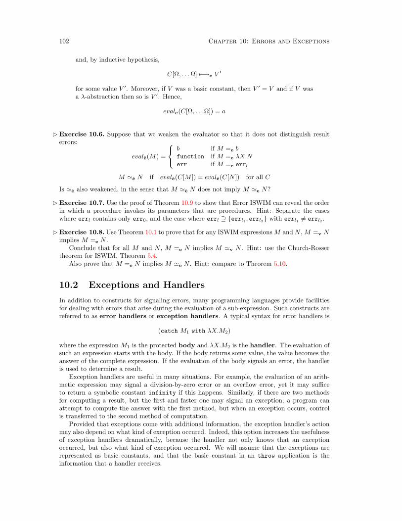
102 Chapter 10: Errors and Exceptions
and, by inductive hypothesis,
C[Ω, . . . Ω] 7−→e V ′
for some value V ′. Moreover, if V was a basic constant, then V ′ = V and if V wasa λ-abstraction then so is V ′. Hence,
evale(C[Ω, . . . Ω]) = a
Exercise 10.6. Suppose that we weaken the evaluator so that it does not distinguish resulterrors:
evale(M) =
b if M =e bfunction if M =e λX.Nerr if M =e errl
M 'e N if evale(C[M ]) = evale(C[N ]) for all C
Is 'e also weakened, in the sense that M 'e N does not imply M 'e N?
Exercise 10.7. Use the proof of Theorem 10.9 to show that Error ISWIM can reveal the orderin which a procedure invokes its parameters that are procedures. Hint: Separate the caseswhere errl contains only err0, and the case where errl ⊇ errl1 , errl2 with errl1 6= errl2 .
Exercise 10.8. Use Theorem 10.1 to prove that for any ISWIM expressions M and N , M =v Nimplies M =e N .
Conclude that for all M and N , M =e N implies M 'v N . Hint: use the Church-Rossertheorem for ISWIM, Theorem 5.4.
Also prove that M =e N implies M 'e N . Hint: compare to Theorem 5.10.
10.2 Exceptions and Handlers
In addition to constructs for signaling errors, many programming languages provide facilitiesfor dealing with errors that arise during the evaluation of a sub-expression. Such constructs arereferred to as error handlers or exception handlers. A typical syntax for error handlers is
(catch M1 with λX.M2)
where the expression M1 is the protected body and λX.M2 is the handler. The evaluation ofsuch an expression starts with the body. If the body returns some value, the value becomes theanswer of the complete expression. If the evaluation of the body signals an error, the handleris used to determine a result.
Exception handlers are useful in many situations. For example, the evaluation of an arith-metic expression may signal a division-by-zero error or an overflow error, yet it may sufficeto return a symbolic constant infinity if this happens. Similarly, if there are two methodsfor computing a result, but the first and faster one may signal an exception; a program canattempt to compute the answer with the first method, but when an exception occurs, controlis transferred to the second method of computation.
Provided that exceptions come with additional information, the exception handler’s actionmay also depend on what kind of exception occured. Indeed, this option increases the usefulnessof exception handlers dramatically, because the handler not only knows that an exceptionoccurred, but also what kind of exception occurred. We will assume that the exceptions arerepresented as basic constants, and that the basic constant in an throw application is theinformation that a handler receives.

10.2 Exceptions and Handlers 103
Handler ISWIM extends plain ISWIM with throw and catch forms:
M = . . . same as plain ISWIM| (throw b)| (catch M with λX.M)
C = . . . same as plain ISWIM| (catch C with λX.M)| (catch M with λX.C)
For an illustration of the versatility of exception handlers, we consider a procedure that multi-plies the elements of a list of numbers. A naive version of the procedure traverses the list andmultiplies the elements one by one:
Π .= Yv(λπ. λl. (if0 (isnull l) d1e
(∗ (car l) (π (cdr l)))))
In Handler ISWIM, the procedure can check for an occurrence of d0e in the list and can exitthe potentially deep recursion immediately, because the result will be d0e. Exiting can beimplemented by raising an exception that is handled by a surrounding handler:
Π0 .= λl.(catch (Π′ l) with λx.x)
whereΠ′ .= Yv(λπ. λl. (if0 (isnull l) d1e
(if0 (car l) (throw d0e)(∗ (car l) (π (cdr l)))))
In this example, signaling an exception indicates that the proper result was found, and thusspeeds up the ordinary computation.
10.2.1 Calculating with Handler ISWIM
The calculus for Handler ISWIM must clearly incorporate the basic axioms for procedures andprimitive operations of the Error ISWIM calculus. Also, errors should still eliminate pendingcomputations except for error handlers. However, the notion of a pending computation haschanged, and it now depends on the behavior of catch expressions. During the evaluation ofthe protected body, the rest of the evaluation temporarily means the rest of the evaluation ofthe body. If this evaluation process returns a value, this value is the result of the entire catchexpression. Othwerwise, if the second evaluation signals an error, the error is not propagated;instead, the handler is applied to the basic constant associated with the error.
The formal characterization of this sketch is straightforward. Returning a value from theevaluation of the body corresponds to a notion of reduction that returns the first sub-expressionof a handler expression when both sub-expressions are values:
(catch U with λX.M)→ U
A notion of reduction that describes the error handling component of the behavior says that ifthe first sub-expression reduces to a throw expression, its basic constant becomes the argumentof the handler:
(catch (throw b) with λX.M)→ ((λX.M) b)
No other reductions dealing with catch expressions are needed. The second notion of reductionalso points out that the hole of an evaluation context, which represents the pending computationof a redex, cannot be inside the body of a catch expression. Otherwise, error propagationthrough evaluation contexts would circumvent error handlers.

104 Chapter 10: Errors and Exceptions
The notions of reduction for error elements have the almost same shape as the ones for ErrorISWIM. The following defines the calculus for Handler ISWIM. To deal with exceptions raisedby primitive operators, we assume a bijection EM mapping members of errl to members of b,and we change δerr accordingly. We also change the evaluation function to include informationabout the basic constant raised for an escaping exception.
(om b1 . . . bm) δerr (throw b) if δ(om, b1, . . . bm) = errl
and where b = EM(errl)(om V1 . . . (λX.N) . . . Vm) δerr (throw b) where b = EM(errom)(b V ) δerr (throw b′) where b′ = EM(errb)
E[(throw b)] throw (throw b)(catch V with λX.M) return V(catch (throw b) with λX.M) catch ((λX.M) b)
h = βv ∪ δ ∪ δerr ∪ throw ∪ return ∪ catch
Ah = b ∪ function ∪ errb
evalh(M) =
b if M =h bfunction if M =h λX.Nerrb if M =h (throw b)
10.2.2 Consistency for Handler ISWIM
Theorem 10.12 [Consistency with Handlers]: The relation evalh is a partialfunction.
Proof for Theorem 10.12: The relations catch and return trivially satisfy thediamond property. It is also straightforward to show that the proof of the dimaondproperty for the notion of reduction e (but using throw instead of error) extendsto the full syntax. If the reduction based on eltn commutes with the one based oncatch and return, we have the diamond property for the full language. To provethe commutativity of catch and return with the old reductions, there are two cases
• Case C[(catch (throw b) with λX.M)]→ C[((λX.M) b)]Then, a reduction step according to one of δ, βv, δerr, or r either modifies thecontext C or the handler V :
– Case C[(catch (throw b) with λX.M)]→ C ′[(catch (throw b) with λX.M)]The common contractum for C ′[(catch throw b with λX.M)] and C[((λX.M) b)]is C ′[((λX.M) b)].
– Case C[(catch (throw b) with λX.M)]→ C[(catch (throw b) with λX.M ′)]In this case, the expressions reduce to C[((λX.M ′) b)].
In both cases, the reductions to the common contractum always require onestep, which shows that the one-step reduction relations and hence their tran-sitive closures commute.

10.2 Exceptions and Handlers 105
• Case C[(catch U with λX.M)]→ C[U ]In this case, a reduction can affect C, U , and V , which requires an analysis ofthree subcases. Otherwise the proof of this case proceeds as the first one.
The consistency of the calculus and the functionhood of evalh directly follow fromthe diamond property according to the familiar proof strategy.
10.2.3 Standard Reduction for Handler ISWIM
The definition of a deterministic evaluation function for Handler ISWIM can no longer rely onthe simple algorithm for ISWIM and Error ISWIM. We need a revised notion of evaluationcontexts, because we need to be able to reduce the body expression in
(catch ((λx.x) d0e) with λx.x)
However, we do not want to extend the definition of E with (catch E with λX.M), becausethat would allow
(catch (throw b) with λx.x)→ (throw b)
by throw.The solution is to define a new kind of evaluation context, Eh. Meanwhile, unlike in ISWIM
or Error ISWIM, E contexts do not represent the entire rest of a computation relative to aredex. Instead, they only represent rest of the computation up to the closest catch expression.An Eh context will represent the rest of the computation, including all the pending catchexpressions.
Eh = [ ]| (Eh M)| (V Eh)| (om V1 . . . Vi−1 Eh Mi+1 . . . Mm)| (catch Eh with λX.M)
As with Error ISWIM, we must define the standard reduction relation so that it avoids ambi-guities due to multiple matching throw reductions. Instead of one special rule, two are needed;one for an uncaught exception, and one within a catch expression:
E[(throw b)] 7−→h (throw b)Eh[(catch E[(throw b)]
with λX.M)]7−→h Eh[(catch (throw b)
with λX.M)]
The complete definition follows.
h = βv ∪ δ ∪ δerr ∪ return ∪ catch
Eh[M ] 7−→h Eh[N ] if M hNE[(throw b)] 7−→h (throw b)Eh[(catch E[(throw b)]
with λX.M)]7−→h Eh[(catch (throw b)
with λX.M)]
evalsh(M) =
b if M 7−→→h bfunction if M 7−→→h λX.Nerrb if M 7−→→h (throw b)

106 Chapter 10: Errors and Exceptions
The correctness proof of this new specification of the evaluator consists of the usual steps,though it is more complex to show the “unique partitioning” lemma. The redex grammar Mrh
for the lemma omits throw expressions.
Mrh = (V V )| (om V . . . V )| (catch V with λX.M)| (catch (throw b) with λX.M)
Lemma 10.13 [Unique Standard Contexts]: For every closed Handler ISWIMexpression M , one of the following is true for a unique Eh, E, and Mrh:
• M is a value.• There exist a standard context Eh and a standard redex Mrh such that M =
Eh[Mrh].• There exists a context E such that M = E[(throw b)].• There exist a standard context Eh and context E such that M = Eh[(catch E[(throw b)] with λX.M)].
Second, we must show that the evaluator based on the standard reduction function is equal tothe evaluator based on the calculus. We state the theorem without proof.
Theorem 10.14: evalsh = evalh
10.2.4 Observational Equivalence of Handler ISWIM
Observational equivalence of Handler ISWIM is defined as usual.
M 'h N if evalh(C[M ]) = evalh(C[N ]) for all C
It is obvious that any ISWIM expressions that can be distinguished in Error ISWIM can alsobe distinguished in Handler ISWIM. Moreover, the result of these distinguishing programs doesnot have to be an error anymore. With error handlers, all error results can be turned into basicconstants.
Theorem 10.15: M 'e N implies M 'h N . Moreover, the analogue of Theo-rem 10.10 does not hold for Handler ISWIM.
Proof for Theorem 10.15: The first part is trivial. For the second part, assumethat C is a distinguishing context in Error ISWIM for M and N . Take
C ′ = (catch C with λx.x)
as the distinguishing context in Handler ISWIM.
Conjecture 10.16: M 'h N implies M 'e N .
Conjecture 10.17: (M,N) |M 'v N and M 6'e N is the same as (M,N) |M 'v
N and M 6'h N .
Note: The first conjecture implies the second.
Exercise 10.9. Suppose that we weaken the evaluator so that it does not distinguish resulterrors:
evalh(M) =
b if M =h bfunction if M =h λX.Nerr if M =h (throw b)

10.3 Machines for Exceptions 107
M 'h N if evalh(C[M ]) = evalh(C[N ]) for all C
Is 'h also weakened, in the sense that M 'h N does not imply M 'h N?
Exercise 10.10. Here is an even weaker evaluator for Handler ISWIM:
eval3(M) =
b if M =h bfunction if M =h λX.Nb if M =h (throw b)
It differs from the original evaluator in that it maps all programs to basic constants or function.In particular, the modified evaluator ignores the difference between errors and basic constants.
Check that the modified evaluator is still a function. Are the two observational equivalencerelations, defined by evalh and eval3, the same?
10.3 Machines for Exceptions
As we saw in previous chapters, a textual abstract machine, like the standard reduction function,is a good tool for understanding and analyzing the mechanical behavior of programs. It is morealgorithmic than a calculus, yet it avoids the use of auxiliary data structures like activationrecords, stacks, etc. For a good implementation, though, is still too abstract, hiding too manyinefficiencies, so we have also looked at more concrete machines, such as the CC machine.Starting from the standard reduction function for Handler ISWIM, we briefly sketch the changesto the CC machine for ISWIM that are necessary to accomodate errors and error handlers.
10.3.1 The Handler-Extended CC Machine
The rules for 7−→h in Section 10.2.3 (page 105) are an extension of the rules for 7−→v. The basicdifference is that 7−→h distinguishes two notions of the rest of a computation; an evaluationcontext represents the rest of the computation up to the closest catch expression, and a standardredex denotes the rest of the entire computation relative to some standard redex.
A naive adaptation of the strategy of the CC machine suggests a separation of the standardcontext from the control string to avoid the repeated partitioning task. Machine states for therevised CC machine will be pairs consisting of closed expressions and standard contexts. Theinstructions shift information from the control string to the context until a standard redex isfound. If the standard redex is a δ- or a βv-redex, the machine proceeds as before. If the redex isa δerr-redex, the machine places an appropriate throw expression in its control register. Finally,if the control string is an err expression, then the machine erases an appropriate portion of thestandard context: up to the closest handler, if it exists, or the entire context otherwise.
The following rules extend a variant of 7−→cc where each E in the original set of rules isreplaced by Eh:
〈M,Eh〉 7−→cc 〈(throw b), Eh〉 [cc7]
if M δerr (throw b)〈(throw b), E〉 7−→cc 〈(throw b), [ ]〉 [cc8]
〈(catch M with λX.N), Eh〉 7−→cc 〈M,Eh[(catch [ ] with λX.N)]〉 [cc9]
〈V,Eh[(catch [ ] with λX.N)]〉 7−→cc 〈V,Eh〉 [cc10]
〈(throw b), Eh[(catch E with λX.N)]〉 7−→cc 〈(throw b), Eh[(catch [ ] with λX.N)]〉 [cc11]
〈(throw b), Eh[(catch [ ] with λX.N)]〉 7−→cc 〈((λX.N) b), Eh〉 [cc12]
evalcc+h(M) =
b if 〈M, [ ]〉 7−→→cc 〈b, [ ]〉function if 〈M, [ ]〉 7−→→cc 〈λX.N, [ ]〉errb if 〈M, [ ]〉 7−→→cc 〈(throw b), [ ]〉

108 Chapter 10: Errors and Exceptions
For a proof of correctness of this machine, it suffices to check that the six new transitionsfaithfully implement the five new standard reduction transitions. This check is a straightforwardexercise.
Theorem 10.18: evalcc+h = evalsh
Exercise 10.11. Prove Theorem 10.18.
Exercise 10.12. Prove that it is possible to eliminate [cc8] by wraping the initial program in ahandler.
10.3.2 The CCH Machine
One major bottleneck of the naive CC machine for Handler ISWIM is obvious. Althoughthe machine maintains the standard context as a separate data structure, the transition im-plementing error must perform a complex analysis of this data structure. More precisely, itmust partition the standard context to determine the “current” evaluation context, that is,the largest possible evaluation context surrounding the hole. This traversal of the standardcontext, however, is a repetition of the traversal that the machine performed in the search ofthe redex. If it kept the current evaluation context around as a separate data structure, theerror instruction could simply replace the current evaluation context with an empty context.
The idea of separating the “current” evaluation context from the rest of the standard contextsuggests that the entire standard context be represented as a stack of evaluation contexts. Eachelement is the evaluation context between two currently active catch expressions. In order tohandle errors correctly, the evaluation contexts should be paired with their respective handlers.When the machine encounters a catch expression, it pushes the current evaluation context andthe new handler on the stack:
〈(catch M with λX.N), E, H〉 → 〈M, [ ], 〈λX.N, E〉 H〉
When the body of a catch expression is eventually reduced to a value, the machine pops thestack
〈V, [ ], 〈λX.N, E〉H〉 → 〈V,E, H〉
that is, it throws away the current handler and reinstalls the surrounding evaluation context.The instruction for handling errors is analoguous. The H register is a stack of handler–contextpairs:
H = ε| 〈λX.M, E〉 H
We call the new machine the CCH machine, where the “H” stands for “handler stack.” Thefirst six CC instructions, the ones for for plain ISWIM expressions, essentially remain the same;they do not use the additional register in any way and do not alter it. (The handler-extendedCC machine uses Eh in place of E for the original CC rules, but the CCH machine continuesto use E in the rules, because the handler part of the context has been moved into the handlerstack, H.)

10.3 Machines for Exceptions 109
〈(MN), E, H〉 7−→cch 〈M,E[([ ] N)],H〉 [cch1]
if M 6∈ V〈(V M), E, H〉 7−→cch 〈M,E[(V [ ])],H〉 [cch2]
if M 6∈ V〈(on V1 . . . Vi M N . . .), E, H〉 7−→cch 〈M,E[(on V1 . . . Vi [ ] N . . .)],H〉 [cch3]
if M 6∈ V〈((λX.M) V ), E, H〉 7−→cch 〈M [X ← V ], E, H〉 [cchβv]
〈(om b1 . . . bm), E, H〉 7−→cch 〈V,E, H〉 [cchδv]
where δ(om, b1, . . . bm) = V〈V,E[(U [ ])],H〉 7−→cch 〈(U V ), E, H〉 [cch4]
〈V,E[([ ] N)],H〉 7−→cch 〈(V N), E, H〉 [cch5]
〈V,E[(on V1 . . . Vi [ ] N . . .)],H〉 7−→cch 〈(on V1 . . . Vi V N . . .), E, H〉 [cch6]
〈M,E,H〉 7−→cch 〈(throw b), E, H〉 [cch7]
if Mδerr(throw b)〈(throw b), E, H〉 7−→cch 〈(throw b), [ ],H〉 [cch8]
〈(catch M with λX.N), E, H〉 7−→cch 〈M, [ ], 〈λX.N, E〉 H〉 [cch9]
〈V, [ ], 〈U, E〉 H]〉 7−→cch 〈V,E, H〉 [cch10]
〈(throw b), E, H〉 7−→cch 〈(throw b), [ ],H〉 [cch11]
〈(throw b), [ ], 〈U, E〉 H〉 7−→cch 〈(U b), E, H〉 [cch12]
evalcch(M) =
b if 〈M, [ ], ε〉 7−→→cch 〈b, [ ], ε〉function if 〈M, [ ], ε〉 7−→→cch 〈λX.N, [ ], ε〉errb if 〈M, [ ], ε〉 7−→→cch 〈(throw b), [ ], ε〉
For a correctness proof of the CCH machine, we must find a relationship between the statesof the extended CC machine and those of the CCH machine. The idea for the conversions isthe above-mentioned representation invariant: the standard context of a CC machine state isrepresented as a stack of handlers and evaluation contexts. Conversely, given such a stack, wecan simply create a single standard context that creates the stack. Based on this idea, it is easyto prove the equivalence between the two machines.
Theorem 10.19: evalcch = evalcc+h
Exercise 10.13. Prove Theorem 10.19.
Exercise 10.14. Implement the extended CC and CCH machines.
Exercise 10.15. Derive extended CK and CEK machines based on the CCH machine.
Exercise 10.16. Design a modified CCH machine that reserves a new register for the currenterror handler. Prove its equivalence with the above CCH machine.

110 Chapter 10: Errors and Exceptions

111
Chapter 11: Imperative Assignment
In an imperative language, implementing a loop typically requires variable assignment. Forexample, the following C implementation of sum assigns to the variables n and i:
int sum(int n) int i = 0;while (n > 0) i = i + n;n = n - 1;
return i;
In a purely functional style, we can implement the same loop using tail recursion and accumu-lator arguments, as in the following Scheme function:
(define (sum n i)(if (zero? n)
i(sum (- n 1) (+ i n))))
In general, however, state is not so easily eliminated. Adding assignments or mutation operatorsprovides a whole new set of interesting programming paradigms, especially when added tolanguages with higher-order procedures and complex data structures. In such a language,programs can create, manipulate, and alter cyclic data structures and recursive nestings ofprocedures. A program can also create a kind of “object”: a bundle consisting of data andprocedures for changing the data in the bundle, where other parts of the program can onlyinspect or change the data through the procedures.
In this chapter, we extend ISWIM to accomodate state directly. The encoding of state forloops, as above, suggests a way of handling state in a machine that manipulates text insteadof memory locations. Just as the state in n and i from the C program above is emulated bypassing arround n and i Scheme variables, we will model state in general as an entity that ispassed around in the evaluator.
The idea of state flows most naturally from a machine point of view, so we approach a modelof state in terms of a machine.
11.1 Evaluation with State
To model state, we extend the syntax of ISWIM expressions with a assignment expression:
M = . . . same as plain ISWIM| (:= X M)
When a language provides assignment statements for identifiers, the nature of identifiers nolonger resembles that of mathematical variables. A mathematical variable represents somefixed value, but assignable identifiers denote a varying association between names and values.We call the association of an identifier with a current value as its state and refer to the executionof assignments as state changes.
Evaluating the expression ((λx.((λy.x) (:= x (+ x d1e)))) d12e) must therefore proceedroughly like the following:

112 Chapter 11: Imperative Assignment
((λx.((λy.x) (:= x (+ x d1e)))) d12e)→ ((λy.x) (:= x (+ x d1e))) with x = d12e
→ ((λy.x) (:= x (+ d12e d1e))) with x = d12e
→ ((λy.x) (:= x d13e)) with x = d12e
→ ((λy.x) void) with x = d13e
→ x with x = d13e, y = void→ d13e
From the above example, we get two clues about how to model state:
• We cannot use simple substitution when applying a function to an argument. For ex-ample, if we replaced every x with d12e, we would end up with an ill-formed expression(:= d12e (+ d12e d1e)), and we wouldn’t know which d12es to replace with d13es later.
• Instead of rewriting an expression to an expression on each evluation step, we rewrote apair on each step: an expression and a mapping from variables to values.
We might try to model := using an expression–environment pair, but our experience with CEKsuggests that we shouldn’t try to think of the variable mapping as exactly an environment; todeal with closures, we made a textual “copy” of the environment in each closure. Such copieswould defeat the central mapping in the above example that made assignment work, because(λx.y) would have its own separate environment for x.
The solution is to think of memory as a new slot in the machine. Function applicationselects an unused slot in memory, and replaces all instances of the variable with the slot address.Meanwhile, variable lookup is replaced by slot lookup, and assignment corresponds to changingthe value of a slot. The collection of slots is called a store.
To refine our above sketch, we rewrite expression-store pairs using a set of slot names σ:
〈 ((λx.((λy.x) (:= x (+ x d1e)))) d12e) , 〉→ 〈 ((λy.σ1) (:= σ1 (+ σ1
d1e))) , 〈σ1,d12e〉 〉
→ 〈 ((λy.σ1) (:= σ1 (+ d12e d1e))) , 〈σ1,d12e〉 〉
→ 〈 ((λy.σ1) (:= σ1d13e)) , 〈σ1,
d12e〉 〉→ 〈 ((λy.σ1) void) , 〈σ1,
d13e〉 〉→ 〈 σ1 , 〈σ1,
d13e〉, 〈σ2, void〉 〉→ 〈 d13e , 〈σ1,
d13e〉, 〈σ2, void〉 〉With this approach, we must extend ISWIM again to allow store addresses as expressions, andalso to support the void value generated by an assignment. We do not expect an evaluatableprogram to contain σ or void initially, but reduction steps create store addresses and void inexpression positions.
M = . . . same as plain ISWIM| (:= X M)| σ| (:= σ M)| void
V = . . . same as plain ISWIM| void
C = . . . same as plain ISWIM| (:= X C)
E = . . . same as plain ISWIM| (:= X E)
σ = a store addressΣ = a function 〈σ, V 〉, . . .
FV( (:= X M) ) = X ∪ FV(M)

11.1 Evaluation with State 113
Note that a store address is not a value, which means that when a variable (replaced by a storeaddress) is used as an argument to a function, we must extract the value from the store beforeapplying the function. That’s the behavior we want for a call-by-value language, as opposed toa call-by-reference language.
To define evaluation, we define the CS machine, which transforms expression-store pairs〈M,Σ〉:
〈E[((λX.M) V )],Σ〉 7−→cs 〈E[M [X ← σ]],Σ[σ ← V ]〉 [csβs]
where σ 6∈ dom(Σ)〈E[σ],Σ〉 7−→cs 〈E[V ],Σ〉 [cs1]
where V = Σ(σ)〈E[(:= σ V )],Σ[σ ← V ′]〉 7−→cs 〈E[void],Σ[σ ← V ]]〉 [cs2]
〈E[(on V1 . . . Vn)],Σ〉 7−→cs 〈E[V ],Σ〉where V = δ(on, V1, . . . Vn) [csδ]
evalcs(M) =
b if 〈M, ∅〉 7−→→cs 〈b, Σ〉function if 〈M, ∅〉 7−→→cs 〈λX.N, Σ〉void if 〈M, ∅〉 7−→→cs 〈void,Σ〉
To make examples easier to read, we introduce two macros:
(let X = M in N) .= ((λX.N) M)
(begin M N) .= (let X = M in N)
where X 6∈ FV (N)
With these abbreviations, we can write the original example as
(let x = d12e in (begin (:= x d13e) x))
Here’s another example:
〈 let i = d0e
in let f = Yvλf.λx.if0 x
i(begin(:= i (+ i x))(f (− x d1e)))
in(f d1e)
, 〉
7−→→cs 〈 let f = Yvλf.λx.if0 x
σ1
(begin(:= σ1 (+ σ1 x))(f (− x d1e)))
in(f d1e)
, σ1 = d0e〉
7−→→cs 〈(σ2d1e) , σ1 = d0e, σ2 = F〉

114 Chapter 11: Imperative Assignment
where F =the value of Yvλf.λx.if0 x
σ1
(begin(:= σ1 (+ σ1 x))(f (− x d1e)))
7−→→cs 〈 if0 σ4
σ1
(begin(:= σ1 (+ σ1 σ4))(σ3 (− σ4
d1e)))
, σ1 = d0e, σ2 = F, σ3 = F, σ4 = d1e〉
7−→→cs 〈 (begin(:= σ1 (+ σ1 σ4))(σ3 (− σ4
d1e)))
, σ1 = d0e, σ2 = F, σ3 = F, σ4 = d1e〉
7−→→cs 〈 (begin(:= σ1 (+ d0e d1e))(σ3 (− σ4
d1e)))
, σ1 = d0e, σ2 = F, σ3 = F, σ4 = d1e〉
7−→→cs 〈 (σ3 (− σ4d1e)) , σ1 = d1e, σ2 = F, σ3 = F, σ4 = d1e〉
7−→→cs 〈 (σ3d0e) , σ1 = d1e, σ2 = F, σ3 = F, σ4 = d1e〉
7−→→cs 〈 if0 σ6
σ1
(begin(:= σ1 (+ σ1 σ6))(σ5 (− σ6
d1e)))
, σ1 = d1e, σ2 = F, σ3 = F, σ4 = d1e,σ5 = F, σ6 = d0e 〉
7−→→cs 〈 σ1, σ1 = d1e, σ2 = F, σ3 = F, σ4 = d1e,σ5 = F, σ6 = d0e 〉
7−→→cs 〈 d1e, σ1 = d1e, σ2 = F, σ3 = F, σ4 = d1e,σ5 = F, σ6 = d0e 〉
11.2 Garbage Collection
In the preceding example, the evaluator must allocate two new slots in the store whenever Fis called: one for the f argument and one for x. (Actually, more slots; the trace above ignoresthe extra arguments introduced by Yv.) But after F makes a recursive call, neither of theslots is ever used again. For example, σ2 is never used in the second half of the evaluation.At some point, we could have easily predicted that σ2 will never be used again; inspecting theexpression and store half-way through the evaluation, we could see that σ2 is not reachablefrom the expression.
In contrast, σ1 is used all the way to the end of the evaluation. At the point where theexpression to evaluate is (σ3 0), σ1 does not appear in the expression. However, σ3 containsthe expression F , and F includes a reference to σ1. Thus, even at the expression (σ3 0), we cansee that σ1 might be used again.
Since we might want to run the example program for an input much larger than 1, anevaluator for our language must somehow forget about useless slots. Otherwise, a program thatwe expect to run in constant space will keep accumulating slots on each function call.
Forgetting unused slots is the essence of garbage collection in languages like Java andScheme. We can formalize the notion of garbage collection within our language by defining the

11.2 Garbage Collection 115
live slots LS of an expression and state as follows:
LS(σ) = σLS(b) = ∅LS(X) = ∅LS(void) = ∅LS( (λX.M) ) = LS(M)LS( (M1 M2) ) = LS(M1) ∪ LS(M2)LS( (on M1 . . . Mn) ) = LS(M1) ∪ . . .LS(Mn)LS( (:= X M) ) = LS(M)
LS(〈M, 〈σ1, V1〉, . . . 〈σn, Vn〉〉) = LS(M) ∪ LS(V1) ∪ . . .LS(Vn)
Any σ that is in dom(Σ) but not in LS(〈M,Σ〉) is a garbage slot. We can add a rule to 7−→cs
that removes a set of garbage slots:
〈M,Σ[σ1 ← V1] . . . [σn ← Vn]〉 7−→cs 〈M,Σ〉 [csgc]
if σ1, . . . σn 6∈ LS(〈M,Σ〉)
Adding this rule to 7−→cs makes it non-deterministic in two ways. First, the rule can apply atthe same time as other rules, which means that the programmer does not know when a garbagecollection will occur. Second, the rule could match with different sets of σs, which means thata programmer does not know which slots are freed when a collection does occur.
More importantly, if we ignore memory constraints, an evaluation of M with as manygarbage collection steps as possible will always produce the same result as an evalution of Mwithout any garbage collection steps. In other words, the garbage collector proves that certainslots will never contribute to evaluation, so that it is safe to remove them from the store.
If we consider memory constraints, then we need to ensure that the garbage collection ruleis used often enough, and that it collects enough garbage. One possibility is to change themachine so that a garbage collection occurs with every reduction, and that the resulting Σ isthe smallest possible one after each step; this strategy is similar to requiring that environmentsare pruned on every closure creation (as in Section 8.3). As it turns out, a unique minimal Σexists for each step, so the resulting machine would be deterministic. However, performing agarbage collection after every evaluation step is not a practical implementation. We return tothe question of a practical implementation in Section 11.4.
Exercise 11.1. Revise the evaluation of
let i = d0e
in let f = Yvλf.λx. if0 x i (begin (:= i (+ i x)) (f (− x d1e)))in (f d1e)
in Section 11.1 by inserting a [csgc] step after each of the shown steps. Each [csgc] should producea minimal store.
Exercise 11.2. Suppose that we add a simpler garbage-collection rule to 7−→cs that alwayscollects a single garbage slot:
〈M,Σ[σ ← V ]〉 7−→cs 〈M,Σ〉if σ 6∈ LS(〈M,Σ〉)
Why is this rule generally not sufficient to ensure proper garbage collection? (Hint: Why didwe ignore reference counting as a possible strategy for memory management?) Provide anexpression with the following properties:

116 Chapter 11: Imperative Assignment
1. It loops forever using 7−→cs rules other than [csgc].
2. It loops in bounded space when the [csgc] rule is used occasionally (i.e., never twice inconsecutive steps).
3. It cannot loop in bounded space using the simpler rule above (even if the rule is appliedmultiple times in consecutive steps).
Hint: no plain ISWIM expression meets all three conditions. We introduce garbage collectionin this chapter because we did not need it before.
11.3 CEKS Machine
The CS machine contains none of our earlier refinements over the basic ISWIM textual machine.For every step, it has to find the redex, sometimes perform substitutions over large expressions,etc. We can get all of our old refinements back by starting with the CEK machine and extendingit with state.
Environments for the CEKS machine map variables to slot addresses. Also, since thenew := expression form contains a subexpression, we must extend the continuation grammarκ. Finally, a store in the CEKS machine maps slot addresses to value closures (instead of plainvalues).
E = a function 〈X, σ〉, . . .κ = . . . same as CEK| 〈set, c, κ〉
Σ = a function 〈σ, v〉, . . .
Most of the reduction rules for CEKS are the same as the CEK rules, except that they propagatea store. Function application and variable look are changed, however. In the follow definition,the rules with an asterisk are new or significantly revised compared to the CEK rules:
〈〈(M N), E〉, κ, Σ〉 7−→ceks 〈〈M, E〉, 〈arg, 〈N, E〉, κ〉,Σ〉 [ceks1]
〈〈(on M N . . .), E〉, κ, Σ〉 7−→ceks 〈〈M, E〉, 〈opd, 〈on〉, 〈〈N, E〉, . . .〉, κ〉,Σ〉 [ceks2]
〈〈V, E〉, 〈fun, 〈(λX.M), E ′〉, κ〉,Σ〉 7−→ceks 〈〈M, E ′[X ← σ]〉, κ, Σ[σ ← 〈V, E〉]〉 [ceks3]∗
if V 6∈ X if σ 6∈ dom(Σ)〈〈V, E〉, 〈arg, 〈N, E ′〉, κ〉,Σ〉 7−→ceks 〈〈N, E ′〉, 〈fun, 〈V, E〉, κ〉,Σ〉 [ceks4]
if V 6∈ X〈〈b, E〉,〈opd, 〈〈bi, E i〉 . . . 〈b1, E1〉, on〉,
〈〉, κ〉,Σ〉
7−→ceks 〈〈V, ∅〉, κ, Σ〉 [ceks5]
where δ(on, b1, . . . , bi, b) = V
〈〈V, E〉,〈opd, 〈c′, . . . on〉,
〈〈N, E ′〉, c, . . .〉, κ〉,Σ〉
7−→ceks 〈〈N, E ′〉,〈opd, 〈〈V, E〉, c′, . . . on〉, 〈c, . . .〉, κ〉,Σ〉
[ceks6]
if V 6∈ X〈〈X, E〉, κ, Σ〉 7−→ceks 〈c, κ, Σ〉 [ceks7]∗
where Σ(E(X)) = c〈〈(:= X M), E〉, κ, Σ〉 7−→ceks 〈〈M, E〉, 〈set, 〈X, E〉, κ〉,Σ〉 [ceks8]∗
〈〈V, E ′〉, 〈set, 〈X, E〉, κ〉,Σ〉 7−→ceks 〈〈void, ∅〉, κ, Σ[σ ← 〈V, E ′〉]〉 [ceks9]∗
if V 6∈ X where E(X) = σ
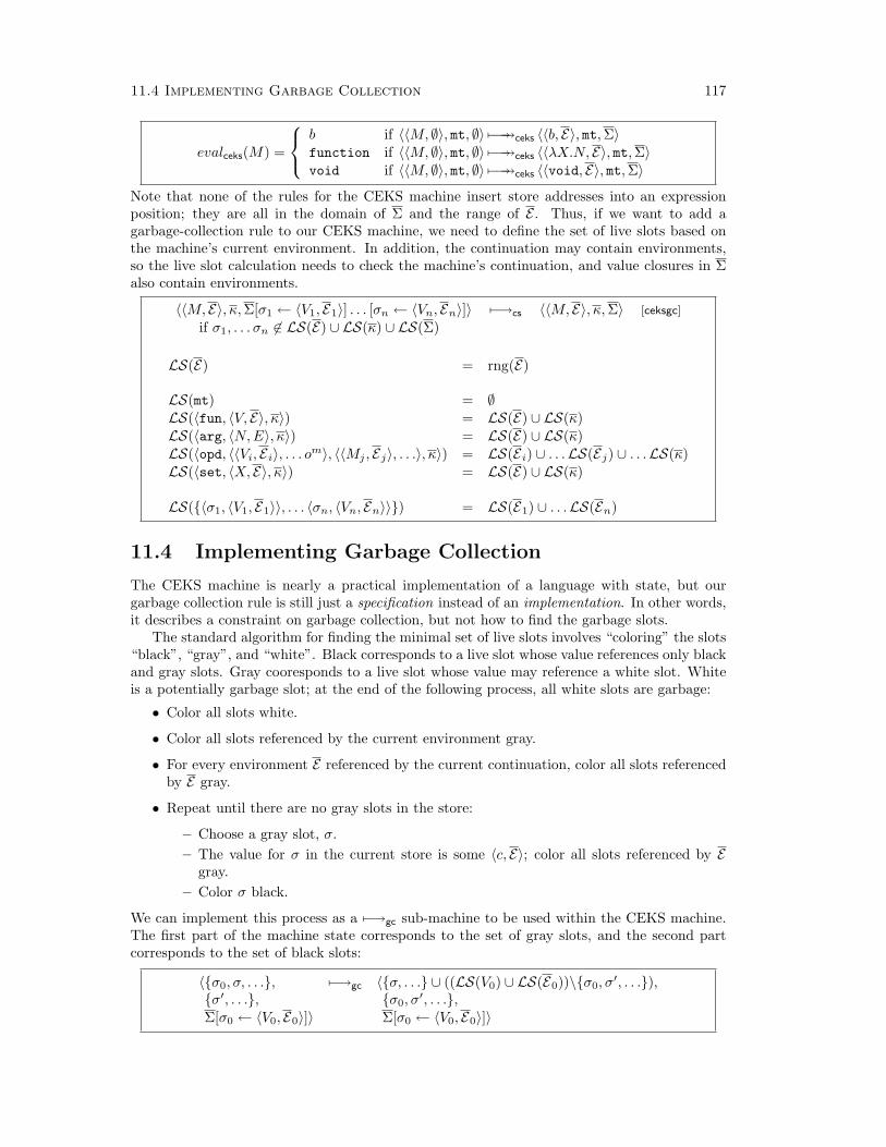
11.4 Implementing Garbage Collection 117
evalceks(M) =
b if 〈〈M, ∅〉, mt, ∅〉 7−→→ceks 〈〈b, E〉, mt,Σ〉function if 〈〈M, ∅〉, mt, ∅〉 7−→→ceks 〈〈λX.N, E〉, mt,Σ〉void if 〈〈M, ∅〉, mt, ∅〉 7−→→ceks 〈〈void, E〉, mt,Σ〉
Note that none of the rules for the CEKS machine insert store addresses into an expressionposition; they are all in the domain of Σ and the range of E . Thus, if we want to add agarbage-collection rule to our CEKS machine, we need to define the set of live slots based onthe machine’s current environment. In addition, the continuation may contain environments,so the live slot calculation needs to check the machine’s continuation, and value closures in Σalso contain environments.
〈〈M, E〉, κ, Σ[σ1 ← 〈V1, E1〉] . . . [σn ← 〈Vn, En〉]〉 7−→cs 〈〈M, E〉, κ, Σ〉 [ceksgc]
if σ1, . . . σn 6∈ LS(E) ∪ LS(κ) ∪ LS(Σ)
LS(E) = rng(E)
LS(mt) = ∅LS(〈fun, 〈V, E〉, κ〉) = LS(E) ∪ LS(κ)LS(〈arg, 〈N,E〉, κ〉) = LS(E) ∪ LS(κ)LS(〈opd, 〈〈Vi, E i〉, . . . om〉, 〈〈Mj , Ej〉, . . .〉, κ〉) = LS(E i) ∪ . . .LS(Ej) ∪ . . .LS(κ)LS(〈set, 〈X, E〉, κ〉) = LS(E) ∪ LS(κ)
LS(〈σ1, 〈V1, E1〉〉, . . . 〈σn, 〈Vn, En〉〉) = LS(E1) ∪ . . .LS(En)
11.4 Implementing Garbage Collection
The CEKS machine is nearly a practical implementation of a language with state, but ourgarbage collection rule is still just a specification instead of an implementation. In other words,it describes a constraint on garbage collection, but not how to find the garbage slots.
The standard algorithm for finding the minimal set of live slots involves “coloring” the slots“black”, “gray”, and “white”. Black corresponds to a live slot whose value references only blackand gray slots. Gray cooresponds to a live slot whose value may reference a white slot. Whiteis a potentially garbage slot; at the end of the following process, all white slots are garbage:
• Color all slots white.
• Color all slots referenced by the current environment gray.
• For every environment E referenced by the current continuation, color all slots referencedby E gray.
• Repeat until there are no gray slots in the store:
– Choose a gray slot, σ.– The value for σ in the current store is some 〈c, E〉; color all slots referenced by E
gray.– Color σ black.
We can implement this process as a 7−→gc sub-machine to be used within the CEKS machine.The first part of the machine state corresponds to the set of gray slots, and the second partcorresponds to the set of black slots:
〈σ0, σ, . . .,σ′, . . .,Σ[σ0 ← 〈V0, E0〉]〉
7−→gc 〈σ, . . . ∪ ((LS(V0) ∪ LS(E0))\σ0, σ′, . . .),
σ0, σ′, . . .,
Σ[σ0 ← 〈V0, E0〉]〉

118 Chapter 11: Imperative Assignment
With the transitive-reflexive closure 7−→→gc , we can redefine the CEKS GC rule as follows:
〈〈M, E〉, κ, Σ〉 7−→cs 〈〈M, E〉, κ, ∅[σ1 ← Σ(σ1)] . . . [σn ← Σ(σn)]〉 [ceksgc]
if 〈LS(M) ∪ LS(E), ∅,Σ〉 7−→→gc 〈∅, σ1, . . . σn,Σ〉
This rule determines a unique and minimal store for a garbage collection step in the CEKmachine. At this point, the only missing part of the specification is a way to ensure that the[ceksgc] rule is used frequently enough.
Exercise 11.3. Implement the CEKS machine. Every other step taken by your CEKS machineshould be a [ceksgc] step that collects as many slots as possible.
11.5 History
The apporach to specifying garbage collection with 7−→gc is due to Morrisett, Felleisen, andHarper [6].

Part III
Models of Typed Languages
119


121
Chapter 12: Types
The text string(+ d1e −)
is not a well-formed ISWIM expression, according to the grammar for M . Consequently, anevaluator for ISWIM need not handle such a text string as its input. The “expression” does notget struck, does not signal an error, and does not loop forever; because it’s not an expressionat all, such claims would be nonsense.
In contrast, the text string(+ d1e (λx.d9e))
is a well-formed ISWIM expression, according to the grammar for M . Nevertheless, it seemsclearly “bad”. It’s immediately obvious that the expression will get stuck if we try to evaluateit, because a function value cannot be provided as an argument to a primitive operation.
In this and the following chapters, we study expression checkers that can detect and reject“bad” expressions before evaluating them. Since we would like to actually implement thechecker, distinguishing good and bad programs should be a mechanical process. Also, we needto explain the checking process to programmers. In particular, we would like take the sort offormal notation that we’ve developed for explaining program executions, and use it to explainprogram checking. In short, we would like to develop a formal view of program checking.
For a formal specification of “good” programs, we might try to refine the grammar M toexclude text strings like (+ d1e (λx.d9e)). Even if such a M can be defined, however, therequired changes would make the grammar especially complex. Extra complexity in M impliescorresponding complexity in proofs and programs over M , so directly modifying the grammar isusually not the best approach. Instead, we will define a separate expression-checking relation.
The new relation will still distinguish good and bad expressions in a purely syntactic andstatic manner, in the same way that a grammar distinguishes text strings that are elements ofa set from those that are not. In other words, although the job of the relation is to distinguishexpressions that evaluate badly from those that evaluate nicely, the checker cannot execute theprogram to make the distintiction. Doing so would defeat the purpose of checking expressionsbefore evaluating them.
Recall that every expression M either
• evaluates to a value;
• gets stuck during evaluation; or
• loops forever.
Since we cannot solve the halting problem, we cannot implement a decision procedure to putan expression into exactly one of these categories; the power of our checking relation will benecessarily limited. The checker can still be useful, though:
• The checker might reject expressions that provably get stuck or loop forever. In that case,when an expression passes the type checker, it might or might not produce a value.
• The checker might accept only expressions that provably produce a value. In that case,when an expression passes the type checker, it will certainly produce a value, but adifferent program that produces a value might be rejected by the checker.
⇒ • The checker might accept only expressions that provably either produce a value or loopforever. In that case, when an expression passes the type checker, it will certainly not getstuck. As in the previous case, a program that produces a value might be rejected by thechecker.

122 Chapter 12: Types
A type relation (or type system) implements the last of the above possibilities. A languagethat consists of an expression grammar, evaluation relation, and type relation is a typedlanguage. Each language that we have studied so far, which comprised only an expressiongrammar and a reduction relation, was an untyped language.
The design of a type system is an open-ended task: since any type system for a realisticlanguage must reject some set of programs that do not get stuck, we can always search foran improved type system that rejects fewer good programs. In this chapter, we begin ourexploration of types with a small language and a simple type checker. In the following chapters,we explore a series of type systems for ISWIM.
12.1 Numbers and Booleans
To start exploring type systems, we begin with a small language of booleans and numbers:
N = t| f| dne
| (+ N N)| (iszero N)| (if N N N)
(+ dne dme) z dn + me
(iszero d0e) z t(iszero dne) z f where n 6= 0(if t N1 N2) z N1
(if f N1 N2) z N2
C = [ ]| (+ C N)| (+ N C)| (iszero C)| (if C N N)| (if N C N)| (if N N C)
E = [ ]| (+ E N)| (+ V E)| (iszero E)| (if E N N)
V = t| f| dne
If we define 7−→z, 7−→→z and evalz in the usual way, then this language has many expressionsthat get stuck. For example:
(+ t d0e)
gets stuck because + doesn’t operate on booleans, and
(if (+ d1e d5e) t d0e)
gets stuck because the test expression for if does not produce a boolean.Since the language for N is not Turing-complete, we could actually define an type checker
based on evaluation. In preparation for more interesting languages, however, we will adopt aless precise strategy that scales to more interesting languages.
The key idea is that programs get stuck because the wrong kind of value flows into a positionwhere the reduction rules inspect the value. The + operator expects numbers, iszero expectsnumbers, and if expects booleans.
We will therefore design a relation that associates expressons with types. Like an expression,a type in the formal sense is a purely syntactic entity. In the same way that we define formalevaluation relations based on an intution of how expressions should be evaluated, we also define

12.1 Numbers and Booleans 123
a formal type relation based on our intutions about the kinds of values that appear duringevaluation.
For our number and boolean language, we first define the set of types T :
T = bool| num
The relation ` : matches expressions with types. Literal boolean expressions have the typebool, and literal numbers have the type num:
` t : bool` f : bool` dne : num
We might also introduce a rule that assigns every addition expression the type num. However,we will use ` : both to describe the kind of value returned by an expression, and to identifyexpressions that cannot get stuck. In other words, we want to design ` : so that if ` N : Tfor some N and T , then N cannot get stuck.
Thus, we want an addition expression to have type num only if its subexpressions also havetype num. The iszero rule is similar, except that it gets the type bool:
` N1 : num ` N2 : num` (+ N1 N2) : num
` N : num` (iszero N) : bool
The only remaining expression form is if. Clearly, the first sub-expression of an if expressionshould have type bool, but the z rule for if makes no requirements on the other expressions.This analysis suggests a rule of the shape:
` N1 : bool` (if N1 N2 N3) :
But what is the type for the entire if expression? If N1 evaluates to t, the result of the ifexpression is the result of N2. If N1 instead evaluates to f, the result of the if expression isthe result of N3. Since we do not want to evaluate N1 to type-check the expression, we areforced to require that N2 and N3 both have the same type, and that type is the one for the ifexpression:
` N1 : bool ` N2 : T ` N3 : T` (if N1 N2 N3) : T
This rule can match with T as bool or as num, but all three instances of T must match thesame type.
At this point, we have a complete set of type rules for N and v. We can see that(if (if t f t) d0e d1e) is categorized as a “good” expression, since ` : assigns it a type:
` t : bool ` f : bool ` t : bool` (if t f t) : bool ` d0e : num ` d1e : num
` (if (if t f t) d0e d1e) : num
In contrast, (if d7e d0e d1e) has no type, since 6` d7e : bool. The following example also has notype:
(if t d1e f)

124 Chapter 12: Types
despite the fact that it reduces via 7−→z to d1e. Our type system is thus conservative in theexpressions it designates as “good”. Whether this conservatism is acceptable depends on aprogrammer’s needs, just like any other aspect of the language.
Lemma 12.1 [Unique Evaluation Context for 7−→z]: If N 6∈ V , then thereexist E and N ′ such that N = E[N ′] and N has one of the following forms:
• (+ V1 V2)
• (iszero V )
• (if V N1 N2)
Lemma 12.2 [Unique Type for N ]: If ` N : T and ` N : T ′, then T = T ′.
Lemma 12.3: If ` C[N ] : T , then ` N : T ′ for some T ′.
Lemma 12.4: If ` C[N ] : T , ` N : T ′, and ` N ′ : T ′, then ` C[N ′] : T .
Exercise 12.1. Prove that ` (if (iszero d3e) (iszero (+ d1e d3e)) t) : bool (i.e., show theproof tree).
Exercise 12.2. Prove Lemma 12.1 (Unique Evaluation Context).
Exercise 12.3. Prove Lemma 12.2 (Unique Type).
Exercise 12.4. Prove Lemma 12.3.
Exercise 12.5. Prove Lemma 12.4.
12.2 Soundness
A typed language is sound if its type system and evaluation rules are consistent, i.e., if the typesystem assigns an expression a type, then the expression does not get stuck when evaluated.
Theorem 12.5 [Soundness of ` : and 7−→→z ]: If ` N : T , then either
• N 7−→→z V , or
• N 7−→→z N ′ implies that N ′ 7−→z N ′′ for some N ′′.
To prove the soundness theorem, we develop a pair of lemmas. The first is a preservation(or subject reduction) lemma that says when 7−→z maps a typed expression to some otherexpression, the expressions have the same type. The second is a progress lemma, which saysthat 7−→z relates every non-V typed expression to some other expression. Together, theselemmas prove the soundness theorem. This technique for proving soundness was developed byWright and Felleisen.
Lemma 12.6 [Preservation for 7−→z]: If N 7−→z N ′ and ` N : T , then ` N ′ : T .
Proof for Lemma 12.6: Since, N 7−→z N ′, there must be some E, N1, andN ′
1 such that N = E[N1] where N1 zN ′1. By Lemma 12.3 there must be some T1
such that ` N1 : T1. Consider all cases for N1 zN ′1, which will prove a sub-claim,
` N ′1 : T1:
• Case (+ dne dme) z dn + me
Since ` dne : num and ` dme : num, ` (+ dne dme) : num so T1 = num. Similarly,` dn + me : num, so the sub-claim holds.

12.2 Soundness 125
• Case (iszero d0e) z tSince ` d0e : num, T1 = bool. Since ` t : bool, the sub-claim holds.• Case (iszero dne) z f
Analogous to the previous case.• Case (if t N2 N3) zN2
By assumption, ` (if t N2 N3) : T1, so whatever T1 is, it must be possible toshow ` N2 : T1. Thus, the sub-claim holds.• Case (if f N2 N3) zN3
Analogous to the previous case.
Finally, by Lemma 12.4, ` E[N ′1] : T , so the original claim holds.
Lemma 12.7 [Progress for 7−→z]: If ` N : T , then either N ∈ V or N 7−→z N ′
for some N ′.
Proof for Lemma 12.7: By induction on the structure of N .
• Base cases:– Case N = t
t ∈ V .– Case N = f
t ∈ V .– Case N = dne
dne ∈ V .• Inductive cases:
– Case N = (+ N1 N2)There are three sub-cases:∗ Case N1 6∈ V
By Lemma 12.1, N1 = E[N0] for some E and N0 6∈ V . By assumption,` (+ N1 N2) : T , which requires ` N0 : T0 for some T0. By induction,N0 7−→z N ′
0; in particular, N0 zN ′0 due to the partitioning of N1 into E
and N0. Let E′ = (+ E N2); then N = E′[N0] and E′[N0] 7−→z E′[N ′0].
∗ Case N2 6∈ VAnalogous to the previous case.
∗ Case N1 = V1, N2 = V2
Since ` (+ N1 N2) : T , ` N1 : num and ` N2 : num. By inspectionof V , we see that the only members of V that have type num arenumbers: dne. Thus, N = (+ dne
1dne
2). By the definition of 7−→z,N 7−→z
dn1 + n2e.
– Case N = (iszero N1)Analogous to the previous case.
– Case N = (if N1 N2 N3)There are two sub-cases:∗ Case N1 6∈ V
This case is analogous to the first sub-case of N = (+ N1 N2).∗ Case N1 = V1
Since ` (if N1 N2 N3) : T , ` N1 : bool. By inspection of V , wesee that the only members of V that have type bool are t and f. IfN1 = t, then N 7−→z N2, and if N1 = f then N 7−→z N3.
Exercise 12.6. Prove Theorem 12.5 (Soundness). Begin by proving a multi-step presevationlemma: If N 7−→→z N ′ and ` N : T , then ` N ′ : T .

126 Chapter 12: Types

127
Chapter 13: Simply Typed ISWIM
We are now ready to consider a typed variant of ISWIM that can reject expressions such as
(+ d1e (λx.d9e))
Our simple language from the previous chapter had exactly two types: bool and num. SinceISWIM is parameterized over the basic constrants and primitive operations, a typed ISWIMwill also be parameterized over the basic types. But, as the expression above illustrates, a typedISWIM will always need at least one type: the type for functions.
In this chapter, we present Simply Typed ISWIM, which illustrates a simple type systemfor functions.
13.1 Function Types
For the sake of concrete examples, we will continue to use the same basic constants and primitiveoperations that we used in previous chapters. Thus, the only basic type we need is num.
We might then define a type system for Simply Typed ISWIM with the following elements:
T = num| function
Such a type system could reject(+ d1e (λx.d9e))
because + will require arguments of type num, and (λx.d9e) will have type function. Butconsider the expression
(+ d1e ( (if0 M (λx.d8e) λxy.y ) d7e))
Both arms of the if0 expression are of type function, so the application expression that usesthe result of the if0 expression could be well-typed. However, the result of the application tod7e will either be a number or the identity function, depending on whether M produces d0e ornot. Thus, the addition expression will potentially get stuck.
The problem is that the type function does not encode enough information about thestructure of a function. Some functions expect numbers, and some expect other functions.Some functions produce numbers, and some produce other functions. The type for a functionneeds to expose this information.
The solution is to support types of the form ( → ). The left-hand side of the arrow specifiesthe type of value that a function consumes, and the right-hand side specified the type of valuethat a function returns. For example, if a function takes a number and produces a number, itstype is (num→ num). If a function takes a number and produces another function from numbersto numbers, its type is (num→ (num→ num)).
The general type grammar for Simply Typed ISWIM is as follows:
T = B| (T → T )
B = a basic type
The set B depends on the basic constants b. For our running example b, we define B to containonly a token for number types:
B = num

128 Chapter 13: Simply Typed ISWIM
Before defining type rules, we must address one more aspect of Simply Typed ISWIM expres-sions. Consider the function
λx.x
Its type might be (num→ num) if we want to use it on numbers, but the function works just aswell on any kind of value, including other functions. Without more information about the kindof value that x is supposed to be, the type rules will have to guess. To avoid this problem (fornow), we modify the expression grammar of Simply Typed ISWIM so that the formal argumentof a function is annotated with an explicit type, indicating the kind of value that the functionexpects to consume. Thus, the above expression must be written as
λx:num.x
for the identity function on numbers, or
λx:(num→ num).x
for the identify function on functions from numbers to numbers.
M = X| (λX:T.M)| (M M)| b| (on M . . . M)
13.2 Type Rules for Simply Typed ISWIM
In the same way that we parameterize Simply Typed ISWIM over its basic constants and theirtypes, we assume an external typing function B for basic constants, and an external function∆ that supplies the expected and result types of primitive operations:
` b : B if B(b) = B
`M1 : B1 . . . `Mn : Bn
` (on M1 . . . Mn) : T where ∆(on) = 〈〈B1, . . . Bn〉, T 〉
For our basic constants and primitive operations, B maps all basic constants to num, and ∆requires num arguments for all operations.
B(b) = num
∆(add1) = 〈〈num〉, num〉∆(sub1) = 〈〈num〉, num〉∆(iszero) = 〈〈num〉, (num→ (num→ num))〉
∆(+) = 〈〈num, num〉, num〉∆(−) = 〈〈num, num〉, num〉∆(∗) = 〈〈num, num〉, num〉∆(↑) = 〈〈num, num〉, num〉
Now that we have rules for basic constants and primitive operations, we need rules for expres-sions of the form X, (λX.M), and (M M).
What type should a variable X have? For evaluation, we never needed to consider thevalue of a variable, because the reduction rules caused (bound) variables to be replaced with

13.2 Type Rules for Simply Typed ISWIM 129
values before the variable itself was evaluated. In the CEK machine, we saw that environmentsprovided an equivalent notion of evaluation without rewriting the body of a function.
For the type checker, we will use an environment to handle variables. This choice emphasizesthat type checking is static (i.e., the type checker only inspects an expression, and does notevaluate it). For type checking, instead of mapping variables to values, a environment Γ mapsvariables to types. We implement the enviornment as a sequence of type associations:
Γ = ε| Γ, X:T
Γ(X) = T if Γ = Γ′, X:TΓ(X) = Γ′(X) if Γ = Γ′, X ′:T and X 6= X ′
The type relation for Simply Typed ISWIM maps pairs Γ and M to a type T , written asΓ ` M : T . For many rules, like the ones for basic constants and primitive operations, theenvironment is simply passed along to type subexpressions, but the environment is consultedto assign a type to a variable.
Γ ` X : T if Γ(X) = TΓ ` b : B if B(b) = B
Γ `M1 : B1 . . . Γ `Mn : Bn
Γ ` (on M1 . . . Mn) : T where ∆(on) = 〈〈B1, . . . Bn〉, T 〉
The type environment must be extended to assign a type to the body of a λ expression. Forexample, the expression
λx:num.(+ x d3e)
is a function, so it should have a type of the form (T → T ). The type for the left-hand sideof the arrow is provided by the programmer: num. To get the type for the right-hand side, wemust check the body expression (+ x d3e) in an environment where x is mapped to num.
More generally, the rule for checking a function expression is as follows:
Γ, X:T `M : T ′
Γ ` (λx:T.M) : (T → T ′)
Finally, the type of an application expression (M N) depends on the kind of value that thefunction M returns. In particular, since M must produce a function, it must have an arrowtype, and the right-hand side of the arrow type determines the result type of the application.Furthermore, the type of N must match the type of argument value expected by M , which isthe left-hand side of the arrow type.
Γ `M : (T ′ → T ) Γ ` N : T ′
Γ ` (M N) : T
The following example illustrates typing with functions, using n as an abbreviation for num:
f :(n→ n) ` f : (n→ n) f :(n→ n) ` d0e : nf :(n→ n) ` (f d0e) : num
` (λf :(n→ n).(f d0e)) : ((n→ n)→ n)
y:num ` y : numy:num ` (add1 y) : num
` (λy:n.(add1 y)) : (n→ n)` ( (λf :(n→ n).(f d0e)) (λy:n.(add1 y)) ) : n

130 Chapter 13: Simply Typed ISWIM
Note that “Γ” never appears in the above proof tree, in the same way that “M” and “T” neverappear. Instead, just as “M” in the rules is replaced by a specific expression, “Γ” is replacedby a specific type environment.
Exercise 13.1. Replace T1, T2, and T3 with specific types in
` (λx:T1.λy:T2.(y x)) d10e (λz:num.(iszero z)) : T3
and prove it (i.e., show the proof tree).
13.3 Soundness
We can prove that our type rules for Simply Typed ISWIM are sound with respect to 7−→v aslong as δ is consistent with B and ∆. In other words, we require the following assumption forany δ, B, and ∆.
Assumption 1 (soundness of primitives):δ(on, b1, ...bn) = V implies ∆(on) = 〈〈B1, . . . Bn〉, T 〉,
B(b1) = B1, . . . B(bn) = Bn,and ` V : T
and∆(on) = 〈〈B1, . . . Bn〉, T 〉,and B(b1) = B1, . . . B(bn) = Bn implies ∃V δ(on, b1, ...bn) = V
With this assumption, we can prove the soundness of Simply Typed ISWIM using the sametechnique as in the previous section: we define and prove Preservation and Progress lemmas.
Theorem 13.1 [Soundness of Simply Typed ISWIM]: If `M : T , then either
• M 7−→→v V , or• M 7−→→v M ′ implies that M ′ 7−→v M ′′ for some M ′′.
Lemma 13.2 [Preservation for Simply Typed ISWIM]: If M 7−→v N and`M : T , then ` N : T .
Lemma 13.3 [Progress for Simply Typed ISWIM]: If ` M : T , then eitherM ∈ V or M 7−→v N for some N .
As before, the above lemmas rely on a set of minor lemmas about unique types and types incontext:
Lemma 13.4: If `M : T and `M : T ′, then T = T ′.
Lemma 13.5: A proof tree for ` C[M ] : T contains a proof tree for Γ `M : T ′ forsome Γ and T ′.
Lemma 13.6: If a proof tree for ` C[M ] : T contains a proof tree for Γ ` M : T ′,then Γ ` N : T ′ implies ` C[N ] : T .
In addition, because the type rules work with type environments while the evalution rulesuse substitution, we need a lemma that relates the types of an expression before and aftersubstitution:
Lemma 13.7: If Γ, X:T ′ `M : T and ` V : T ′, then Γ `M [X ← V ] : T .
Exercise 13.2. Prove Lemma 13.2 (Preservation), assuming the other lemmas above.
Exercise 13.3. Prove Lemma 13.3 (Progress), assuming the other lemmas above.
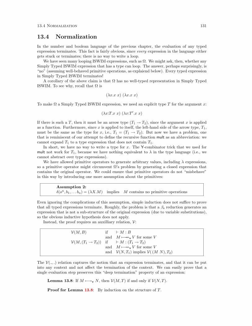
13.4 Normalization 131
13.4 Normalization
In the number and boolean language of the previous chapter, the evaluation of any typedexpression terminates. This fact is fairly obvious, since every expression in the language eithergets stuck or terminates; there is no way to write a loop.
We have seen many looping ISWIM expressions, such as Ω. We might ask, then, whether anySimply Typed ISWIM expression that has a type can loop. The answer, perhaps surprisingly, is“no” (assuming well-behaved primitive operations, as explaiend below). Every typed expressionin Simply Typed ISWIM terminates!
A corollary of the above claim is that Ω has no well-typed representation in Simply TypedISWIM. To see why, recall that Ω is
(λx.x x) (λx.x x)
To make Ω a Simply Typed ISWIM expression, we need an explicit type T for the argument x:
(λx:T.x x) (λx:T ′.x x)
If there is such a T , then it must be an arrow type (T1 → T2), since the argument x is appliedas a function. Furthermore, since x is applied to itself, the left-hand side of the arrow type, T1,must be the same as the type for x, i.e., T1 = (T1 → T2). But now we have a problem, onethat is reminiscent of our attempt to define the recursive function mult as an abbreviation: wecannot expand T1 to a type expression that does not contain T1.
In short, we have no way to write a type for x. The Y-combinator trick that we used formult not work for T1, because we have nothing equivalent to λ in the type language (i.e., wecannot abstract over type expressions).
We have allowed primitive operators to generate arbitrary values, including λ expressions,so a primitive operator might circumvent Ω’s problem by generating a closed expression thatcontains the original operator. We could ensure that primitive operators do not “misbehave”in this way by introducing one more assumption about the primitives:
Assumption 2:δ(on, b1, . . . bn) = (λX.M) implies M contains no primitive operations
Even ignoring the complications of this assumption, simple induction does not suffice to provethat all typed expressions terminate. Roughly, the problem is that a βv reduction generates anexpression that is not a sub-structure of the original expression (due to variable substitutions),so the obvious inductive hypothesis does not apply.
Instead, the proof requires an auxilliary relation, V:
V(M,B) if `M : Band M 7−→→v V for some V
V(M, (T1 → T2)) if `M : (T1 → T2)and M 7−→→v V for some Vand V(N,T1) implies V( (M N), T2)
The V( , ) relation captures the notion that an expression terminates, and that it can be putinto any context and not affect the termination of the context. We can easily prove that asingle evaluation step preserves this “deep termination” property of an expression:
Lemma 13.8: If M 7−→v N , then V(M,T ) if and only if V(N,T ).
Proof for Lemma 13.8: By induction on the structure of T .

132 Chapter 13: Simply Typed ISWIM
• Base case:
– Case T = BIf either M or N terminates, then clearly both terminate with the same V .Furthermore, M and N have the same type by Presevation, so the claimholds.
• Inductive case:
– Case T = (T1 → T2) for some T1 and T2
Assume that V(M,T ), so that M 7−→→v V for some V , and V(N ′, T1) forany N ′ implies V( (M N ′), T2). Clearly N 7−→→v V . Since M 7−→v N , wehave (M N ′) 7−→v (N N ′). Thus, by induction, V( (N N ′), T2).If we assume V(N,T ), we can similarly conclude V(M,T ).
We are now ready to prove the main lemma. The primitive-operation rule can break theinduction we’d like to use, so at first we leave it out. We then prove a similar lemma thatsupports primitive operations, as long as they satisfy Assumptions 1 and 2.
Lemma 13.9: If Γ = X1:T1, . . . Xn:Tn and the following hold:
• M contains no primitive applications,
• Γ `M : T , and
• V(V1, T1), . . . V(Vn, Tn) for some V1, . . ., Vn,
then V(M [X1 ← V1] . . . [Xn ← Vn], T ).
Proof for Lemma 13.9: By induction on Γ `M : T .
• Base cases:
– Case Γ ` X : TX must be some Xi for i ∈ [1, n]. Thus, X[X1 ← V1] . . . [Xn ← Vn] = Vi,and we have assumed V(Vi, T ), so the claim holds.
– Case Γ ` b : TT ∈ B, b[X1 ← V1] . . . [Xn ← Vn] = b, and b ∈ V clearly terminates, sothe claim holds.
• Inductive cases:
– Case Γ ` (λX:T1.N) : TT must be of the form (T1 → T2), where Γ, X:T1 ` N : T2. ClearlyM ′ = M [X1 ← V1] . . . [Xn ← Vn] terminates, since M is a value. Choosean arbitrary N ′ such that V(N ′, T1). To prove the claim, we must showthat V( (M ′ N ′), T2).By the definition of V, N ′ 7−→→v V for some V ; since M ′ is a value, we cansee that (M ′ N ′) 7−→→v (M ′ V ). By βv, this expression reduces further to
N [X1 ← V1] . . . [Xn ← Vn][X ← V ]
That N ′ reduces to V also implies V(V, T1) by a simple multi-step extensionof Lemma 13.8. Combined with Γ, X:T1 ` N : T2 and the inductionhypothesis, we can conclude
V(N [X1 ← V1] . . . [Xn ← Vn][X ← V ], T2)
Again by a multi-step-extended Lemma 13.8, we can conclude V( (M ′ N ′), T2),as desired.

13.4 Normalization 133
– Case Γ ` (M1 M2) : TBy the type rule for application and by induction,
V(M1[X1 ← V1] . . . [Xn ← Vn], (T1 → T ))
andV(M2[X1 ← V1] . . . [Xn ← Vn], T1)
for some T1. Since M1 has an arrow type, by the definition of V,
V( (M1[X1 ← V1] . . . [Xn ← Vn] M2[X1 ← V1] . . . [Xn ← Vn]), T )
We can lift the substitutions out to get the equivalent
V( (M1 M2)[X1 ← V1] . . . [Xn ← Vn], T )
which is what we wanted.– Case Γ ` (om M1 . . . Mm) : T
By assumption, this case cannot occur.
Lemma 13.10: If Γ = X1:T1, . . . Xn:Tn and the following hold:
• Γ `M : T , and
• V(V1, T1), . . . V(Vn, Tn) for some V1, . . ., Vn,
then V(M [X1 ← V1] . . . [Xn ← Vn], T ).
Proof for Lemma 13.10: The proof is analogous to the proof for Lemma 13.9,except that the primitive operation case must be addressed.
• Case Γ ` (om M1 . . . Mm) : T
By the type rules and by induction,
V(M1[X1 ← V1] . . . [Xn ← Vn], B1),. . .V(Mn[X1 ← V1] . . . [Xn ← Vn], Bn)
Thus, M will eventually reduce to (on b1 . . . bm). According to Assumption 1,δ must provide a value V such that ` V : T . According to Assumption 2, Vcontains no primitive operations. Thus, we can apply the weaker Lemma 13.9to conclude V(V, T ). By an extension of Lemma 13.8 and by lifting out subsi-tutions, we can conclude that
V((om M1 . . . Mm)[X1 ← V1] . . . [Xn ← Vn], B1), T )
as desired.

134 Chapter 13: Simply Typed ISWIM

135
Chapter 14: Variations on Simply Typed ISWIM
Since all Simply Typed ISWIM programs terminate, clearly we have lost some expressive powerin the typed version of ISWIM. In particular, we can no longer write recursive programs. As we’llsee in the following sub-sections, we have also lost the ability to encode complex conditionals,or to encode data structures such as pairs.
To recover useful kinds of expressiveness in a typed setting, we can refine the core type rulesso that they allow more programs, including the ones that implement conditionals and pairs.We explore that approach in future chapters.
Meanwhile, in this chapter, we explore a simpler approach: extend Simply Typed ISWIMwith explicit constructs for conditionals, pairs, etc. With these constructs in the language,we can define type rules that work directly on the constructs. In other words, the explicitconstructs provide a place to hang specific type rules that directly reflect our intuition aboutthe constructs.
14.1 Conditionals
In Chapter 12, we defined a language of booleans and numbers with a built-in if form forconditionals. In contrast, for plain ISWIM, we used the encoding or true and false that we firstdeveloped for the pure λ-calculus of Chapter 4, where true is (λx.λy.x) and false is (λx.λy.y).The iszero primitive operation cooperates with this encoding, mapping a number to either(λx.λy.x) or (λx.λy.y), and the if0 macro combines the function encoding of true and falsewith applications to achieve a conditional branch.
For Simply Typed ISWIM, we have to pick typed functions to use for encodings of trueand false. Indeed, when assigning a ∆ mapping for iszero, we implicitly picked a typedencoding; the result type for iszero was defined as (num→ (num→ num)), which is the type of(λx:num.λy:num.x) and (λx:num.λy:num.y). Thus, we can write
((iszero d0e) d1e d2e)
which evaluates to d1e, and is also well-typed. But, unfortunately, we cannot redefine the if0macro to work with this encoding:
(if0 K M N) .= (((iszero K) (λX:num.M) (λX:num.N)) d0e)where X 6∈ FV(M) ∪ FV(N)
The problem is that the first argument to the result of (iszero K) will have a type (num→ ),while the typed encoding of true and false expects an argument of type num. To solve thisproblem, we might choose a different encoding for booleans:
true.= (λx:(num→ num).λy:(num→ num).x)
false.= (λx:(num→ num).λy:(num→ num).y)
In that case, if ∆ gives iszero the result type
((num→ num)→ ((num→ num)→ (num→ num)))
then an expression like (if0 d0e d1e d2e) will have a type:
· · ·` ((iszero d0e) (λx:n.d1e)) : ((n→ n)→ (n→ n))
· · ·` ((λx:n.d2e)) : (n→ n)
` ((iszero d0e) (λx:n.d1e) (λx:n.d2e)) : (n→ n) ` d0e : n` (((iszero d0e) (λx:n.d1e) (λx:n.d2e)) d0e) : n

136 Chapter 14: Variations on Simply Typed ISWIM
Neverthless, the new encoding is still limited. Conditionals using iszero can only be well-typed when they produce numbers. We have lost the ability to write conditionals that producefunctions, as in
(if0 d0e (λx:num.(add1 x)) (λx:num.(sub1 x)))
The easiest way to support such expressions is to add booleans and a conditional form directlyinto Simply Typed ISWIM.
M = . . .| f| t| (if M M M)
T = . . .| bool
∆(iszero) = 〈〈num〉, bool〉
Γ `M1 : bool Γ `M2 : T Γ `M3 : TΓ ` (if M1 M2 M3) : T
Exercise 14.1. Complete the extension of Simply Typed ISWIM for booleans and if, includingnew type rules for t and f, extended definitions for contexts and evaluation contexts, and newevaluation rules to go with βv and δ. Then show that
(if (iszero d0e) (λx:num.(add1 x)) (λx:num.(sub1 x)))
has a type, and that it reduces to a value.
14.2 Pairs
Recall the encoding of pairs from Chapter 4:
mkpair.= λx.λy.λs.(s x y)
fst.= λp.(p λx.λy.x)
snd.= λp.(p λx.λy.y)
The problem with these encodings in a typed setting is similar to the problem with true and false:we have to pick a specific type for x and y in mkpair. Unlike the problem with conditionals,however, no primitive operations are involved that require a fixed type for pairs. We mighttherefore try to define a family of abbreviations, one for each pair of types T1 and T2, whereT1 is the type of the first element in the pair, and T2 is the type for the second element.
mkpair(T1×T2).= λx:T1.λy:T2.λs:(T1 → (T2 → )).(s x y)
fst(T1×T2).= λp:((T1 → (T2 → T1))→ T1).(p λx:T1.λy:T2.x)
snd(T1×T2).= λp:((T1 → (T2 → T2))→ T2).(p λx:T1.λy:T2.y)
This encoding nearly works. The problem is that fst(T1×T2) and snd(T1×T2) must return differentkinds of values if T1 6= T2, but the two functions flow into the same s in mkpair(T1×T2). Thus,there is no good type to put in place of in the definition of mkpair(T1×T2), unless we restrictT1 and T2 to be the same.

14.3 Variants 137
We can solve the problem more generally by adding pairs and pair types directly to SimplyTyped ISWIM. The form 〈M, N〉 pairs the values of M and N together, and the fst and sndforms extract a value from a pair. The type for a pair is (T1 × T2).
M = . . .| 〈M, M〉| (fst M)| (snd M)
V = . . .| 〈V, V 〉
E = . . .| 〈E, M〉| 〈V, E〉| (fst E)| (snd E)
T = . . .| (T × T )
(fst 〈V1, V2〉) p V1
(snd 〈V1, V2〉) p V2v = . . . ∪ p
Γ `M1 : T1 Γ `M2 : T2
Γ ` 〈M1, M2〉 : (T1 × T2)
Γ `M : (T1 × T2)Γ ` (fst M) : T1
Γ `M : (T1 × T2)Γ ` (snd M) : T2
Exercise 14.2. Using both the conditional and pair extensions, show that (fst 〈(add1 d0e), t〉)has a type and a value.
14.3 Variants
Some functions need to accept multiple kinds of values that implement variants of an abstractdatatype. For example, a list-processing function must accept both a constant representing theempty list, null, and a cons cell (cons v l), where v is the first element in the list and l is therest of the list. In addition to accepting both kinds of values, the function must somehow beable to distinguish them.
We can implement such variants in untyped ISWIM by using pairs and attaching a differenttag to each variant. The true tag can identify the empty list, and the false tag can identify acons cell:
null.= 〈true, false〉
cons.= λv.λl.〈false, 〈v, l〉〉
isnull.= λl.fst l
In a typed language, the above encoding does not work. The null constant has the type (bool×bool), whereas a cons cell has type (bool × (T × T ′)) for some T and T ′. These types areincompatible, so we cannot write an isnull function that accepts arguments of both shapes.
Once again, we solve the problem by extending our core language. We will extend it with anotion of variants (or disjoint sums), represented by the type (T1 + T2) for variant types T1
and T2. A value of type (T1 + T2) encapsulates either a value of type T1 or a value of type T2.Three new forms operate on variants of type (T1 + T2): ToLeft(T1+T2), ToRight(T1+T2), and
Match((T1+T2)→T ).
• (ToLeft(T1+T2) M)This form computes the value for M , which must be of type T , and encapsulates it asvalue of type (T1 + T2). In other words, ToLeft(T1+T2) injects a value of type T into(T1 + T2).
• (ToRight(T1+T2) M)This form injects the value of M , of type T2, into (T1 + T2).

138 Chapter 14: Variations on Simply Typed ISWIM
• (Match((T1+T2)→T ) M M1 M2)This form requires M to produce a value of type (T1 + T2). The M1 and M2 expressionsmust each produce a function value; the M1 function must have type (T1 → T ), and theM2 function must have type (T2 → T ). The Match((T1+T2)→T ) form picks an appropriatefunction, depending on whether the value for M encapsulates a value of type T1 or T2. Ifit’s T1, then M1 is invoked with the encapsulated value, otherwise M2 is invoked.
With the new forms, we can take a step towards encoding lists. Lists of arbitrary length requireeven more typing machinery than we have developed so far, but we can at least define a datatypethat encapsulates either an empty list or a “list” containing a single number:
null.= (ToLeft(bool+num) f)
list1.= λv:num.(ToRight(bool+num) v)
isnull.= λl:(bool + num). (Match((bool+num)→bool) l
(λx:bool.t)(λx:num.f))
M = . . .| (ToLeft(T+T ) M)| (ToRight(T+T ) M)| (Match((T+T )→T ) M M M)
V = . . .| (ToLeft(T+T ) V )| (ToRight(T+T ) V )
E = . . .| (ToLeft(T+T ) E)| (ToRight(T+T ) E)| (Match((T+T )→T ) E M M)| (Match((T+T )→T ) V E M)| (Match((T+T )→T ) V V E)
T = . . .| (T + T )
(Match((T1+T2)→T ) (ToLeft(T1+T2) V ) V1 V2) s (V1 V )(Match((T1+T2)→T ) (ToRight(T1+T2) V ) V1 V2) s (V2 V )
v = . . . ∪ s
Γ `M : T1
Γ ` (ToLeft(T1+T2) M) : (T1 + T2)
Γ `M : T2
Γ ` (ToRight(T1+T2) M) : (T1 + T2)
Γ `M : (T1 + T2) Γ `M1 : (T1 → T ) Γ `M2 : (T2 → T )Γ ` (Match((T1+T2)→T ) M M1 M2) : T
Exercise 14.3. using the macro definitions above, show that (isnull (list1 d13e)) has a type anda value.
14.4 Recursion
Using the conditional extension from Section 14.1, we can define a typed version of the mksumfunction:
mksum.= λf :(num→ num).λn:num.(if (iszero n) d0e (+ n (f (sub1 n))))
But we know that Simply Typed ISWIM doesn’t allow recursion, so we should expect that
Yv mksum

14.4 Recursion 139
has no type. Why?Clearly mksum has a type. Applying the type rules we have assigns mksum the type ((num→
num) → (num → num)). In other words, given a function from numbers to numbers, mksumproduces a function from numbers to numbers.
The problem is that Yv itself has no type, for the same reason that Ω has no type. We couldavoid this problem by extending the language with an explicit Yv function and giving it anappropriate type. But since the untyped Yv works on many kinds of functions, we would haveto define a family of Yv functions. One member of the family would create recursive functionsof type (num→ num), another would create functions of type (num→ bool), and so on.
Alternatively, we can add a fix form to the language that acts like Yv, but automaticallyadapts to the target function type. A proto-recursive function (such as mksum) takes a functionof type (T1 → T2) to generate a function of type (T1 → T2). Thus, the type rule for fix is
Γ `M : ((T1 → T2)→ (T1 → T2))Γ ` (fix M) : (T1 → T2)
Since T1 and T2 only appear within (T1 → T2), we can simplify the rule by using T in place of(T1 → T2). The complete extension of the language is as follows:
M = . . .| (fix M)
E = . . .| (fix E)
(fix (λX:T.M)) y M [X ← (fix (λX:T.M))]
v = . . . ∪ y
Γ `M : (T → T )Γ ` (fix M) : T
The y reduction rule implements the essense of the fixed-point equiation directly, so fix cer-tainly acts like Yv. And, using the new type rule we have
· · ·` mksum : ((num→ num)→ (num→ num))
` (fix mksum) : (num→ num)
Thus, (fix mksum) is the recursive multiplication function for a type language.The soundness theorem for Simply Typed ISWIM holds for the langauge extended with fix.
This is easy to see; if (fix (λX:T.M)) has type T , then X can be replaced by (fix (λX:T.M))in M without changing the type of M .
The normalization theorem no longer holds, as demonstrated by the following infinite loop:
((fix λf :(num→ num).λn:num.(f n)) d0e)
Exercise 14.4. Prove that ` (fix (λx:T.x)) : T for any T . How is it possible that (fix (λx:T.x))manufactures a value of type T out of thin air? For example, what number does (fix (λx:num.x))produce when it is evaluated?

140 Chapter 14: Variations on Simply Typed ISWIM

141
Chapter 15: Polymorphism
With the extensions of the previous chapter, we can write many interesting programs in SimplyTyped ISWIM. We cannot necessarily write them as conveniently, however. For example,instead of writing a single identity function
λx.x
we have to write for one every kind of value that we want to use as an argument to the identityfunction
λx:num.xλx:bool.xλx:(num→ num).xλx:((bool→ num) + (num× bool)).x
This duplication of code is wasteful—especially when the function is more complex than identity.In this chapter, we extend our language and type rules so that we can once again write
functions, such as identity, that are polymorphic: they work simultaneously on many kinds(or “shapes”) of data.1
A function that does not inspect its argument in any way is clearly a candidate for poly-morphism, but some functions inspect their arguments only partially. For example, a swapfunction
λp.〈snd p, fst p〉
works only on pair obejcts, but it does not inspect the values in the pair. Thus, this functionis polymorphic, because it works on many different kinds of pairs.
The kind of abstraction that we need over many types is similar to the kind of abstractionthat λ provides over many specific values. This observation suggests that we extend SimplyTyped ISWIM with a mechanism for abstracting an expression over a type, and combining atype-abstracted function with a specific type to get a specific function. The resulting languageis Polymorphic ISWIM. (Note: In the same way that the functional core of ISWIM is calledthe λ-calculus, the functional core of Polymorphic ISWIM is sometimes called System F.)
15.1 Polymorphic ISWIM
To distinguish type abstractions from normal abstractions, we use Λ instead of λ for type ab-stractions. In addition, we keep type identifiers and variable identifiers separate, by designatinga separate set of identifiers for types. Lowercase Roman letters are used for variable identifiers,and lowercase Greek letters for type identifers.
Thus, the polymorphic identify function is
id.= Λα.λx:α.x
where α is a placeholder for an unknown type (in the same way that x is a placeholder for anunknown value).
Along with application for normal functions to values, we need type application for poly-mophic functions to types. We distinguish type applications from normal applications by usinginfix square brackets around a type argument. Thus, to apply id to the number d5e, we write
(id[num] d5e)
1The kinf of polymorhpism that we explore in this chapter is sometimes called parameteric polymorphism.In Chapter 19, we will study a different kind of polymorphism.

142 Chapter 15: Polymorphism
The num type argument gets substituted for α in (λx:α.x) to produce a normal function, whichcan then be applied to d5e in the usual way.
A polymorphic swap function needs two types: one for the first element in the original pair,and one for the second element of the original pair:
swap.= Λα.Λβ.λp:(α× β).〈snd p, fst p〉
By applying the polymorphic swap to num and bool
swap[num][bool]
we obtain a function of type ((num× bool)→ (bool× num)).What is the type of swap itself or of id, in polymorphic form? The id expression is not quite
a function, because it must be applied to type arguments to obtain a function. Nevertheless,the type for id should indicate that it produces a function, and that the type of the functiondepends on the supplied type arguments. To write such types, we use ∀ with a type variable:
` id : (∀α.(α→ α))
Type expressions of this form are called universal types.In the same way that swap contains two Λs, its type contains two ∀s:
` swap : (∀α.(∀β.((α× β)→ (β × α))))
The swap example shows that type expressions, such as (α × β), can include type variables,such as α and β. Thus, our new expression and type grammars are as follows:
M = . . .| (ΛA.M)| M [T ]
V = . . .| (ΛA.M)
T = . . .| A| (∀A.T )
A = a type variable: α, β, . . .
The reduction rules are extended to include type applications:
(ΛA.M)[T ] βt M [A← T ]
v = . . . ∪ βt
where substitution for type variables is defined in the obvious way, and FV(T ) extracts the freetype variables of T in the obvious way.
To assign a type to Polymorphic ISWIM experssions, we need to track type variables inan envionment along with normal variables. Up to now, Γ has mapped normal variables totypes. For Polymorphic ISWIM, we extend Γ so that it also contains type variables. The typevariables have no bindings (the implicit binding would be “is a type”), but they are needed inthe environment to disallow free type variables. For example, the expression
λx:α.x
should not have a type, because α has no meaning, in the same way that the expression
x

15.1 Polymorphic ISWIM 143
without any context has no type. The revised definition of Γ follows:
Γ = ε| Γ, X:T| Γ, A
Γ(X) = T if Γ = Γ′, X:TΓ(X) = Γ′(X) if Γ = Γ′, X ′:T and X 6= X ′
Γ(X) = Γ′(X) if Γ = Γ′, A
Γ(A) if Γ = Γ′, AΓ(A) when Γ′(A) if Γ = Γ′, A′ and A 6= A′
Γ(A) when Γ′(A) if Γ = Γ′, X ′:T
The type rules for type abstraction and type application use the environment with type vari-ables. Furthermore, in expressions with type expressions (including λ expressions), the typeexpression must be checked to ensure that it has no free type variables; the ` relationperforms this check.
Γ, A `M : TΓ ` (ΛA.M) : (∀A.T )
Γ `M : (∀A.T ′) Γ ` TΓ `M [T ] : T ′[A← T ]
Γ, X:T `M : T ′ Γ ` TΓ ` (λX:T.M) : (T → T ′)
Γ ` A if Γ(A) Γ ` B
Γ ` T1 Γ ` T2
Γ ` (T1 → T2) . . . pair types, etc. . . .Γ, A ` T
Γ ` (∀A.T )
Type abstractions introduce yet one more wrinkle into the type-checking process. The type rulefor function application sets up an implicit equation between the type of the argument expres-sion, and the argument type of the function expression. But now that we have Λ abstractionsthat parameterize over an arbitrary type variable, our type grammar includes expressions thatshould be treated the same, but are not syntactically equivalent. For example, (Λα.(α → α))and (Λβ.(β → β)) should be equivalent.
To allow such types to be treated the same, we must modify the application rule to use anexplicit equality check, and we must also define a set of rules ` ↔ for type equivalence.
Γ `M : (T ′ → T ) Γ ` N : T ′′ ` T ′ ↔ T ′′
Γ ` (M N) : T
` T ↔ T` T1 ↔ T ′1 ` T2 ↔ T ′2` (T1 → T2)↔ (T ′1 → T ′2) . . .
` T [A← A′′]↔ T ′[A′ ← A′′]` (∀A.T )↔ (∀A′.T ′) where A′′ 6∈ FV(T ) ∪ FV(T ′)
Exercise 15.1. Show that ` swap : (∀α.(∀β.((α× β)→ (β × α)))).
Exercise 15.2. Although languages with polymorhpism typically also have a built-in notion ofpair, Polymorphic ISWIM supports the pure λ-calculus encoding of pairs, after the encoding isaugmented with appropriate types, Λ abstractions, and type applications. Show this encoding(i.e., show versions of mkpair, fst, and snd that are well-typed in Polymorphic ISWIM).

144 Chapter 15: Polymorphism

145
Chapter 16: Type Inference
Now that we have polymorphism in our language, we can write interesting programs withoutduplicating functionality to satisfy the type system. Nevertheless, the type system still demandsa certain amount of work from the programmer that was not required in plain ISWIM. Forexample, a programmer must write Λ and α in
Λα.λx:α.x
instead of simplyλx.x
to define the polymorphic identity function.In this chapter, we study type inference (or type reconstruction), which relives the
programmer of writing type annotations, but does not sacrifice the benefits of a typed language.The Type-Inferred ISWIM language allows a programmer to write expressions that look likeplain ISWIM, but the expressions are more like Simply Typed ISWIM expressions with all ofthe type abstractions, type applications, and function argument types erased. An inferencephase in Type-Inferred ISWIM effectively reconstructs the erased types and checks the result.Thus, a program in Type-Inferred ISWIM is has a type only if the inferencer can both fill intypes and apply the rules of Simply Typed ISWIM.
After we have developed an inferencer for Simply Typed ISWIM, we can get most of thepower of Polymorphic ISWIM by having the inferencer reconstruct Λ abstractions and typeapplications.
The techniques and notation used in this chapter are derived from Benjamin Pierce’sType Systems for Programming Languages.
16.1 Type-Inferred ISWIM
For Type-Inferred ISWIM expressions, we revert to the original ISWIM grammar without typeannotations:
M = X| (λX.M)| (M M)| b| (on M . . . M)
To define type rules Type-Inferred ISWIM expressions, we might take the rules from SimplyTyped ISWIM and omit the type declarations on function arguments:
Γ, X:T `M : T ′
Γ ` (λx.M) : (T → T ′) . . .
The above is a well-defined rule, but it’s not obviously decidable like the Simply Typed ISWIMrules. In Simply Typed ISWIM, to check a λ expression, a type checker could extend the currenttype environment with the declared argument type, check the body expression in the extendedenvironment, and finally construct a function type using the declared type on the left-hand sideand the body-type on the right-hand side.
Without a declared argument type, a type checker matching the above rule will have to“guess” a T to use as the argument type. For example,
((λx.x) d0e)

146 Chapter 16: Type Inference
The expression above could have type num, where the reconstructed type for the x argument isnum. From this simple example, it might appear that the type rule for application can supplya “guess” to the rule for function by first checking the argument expression, and then usingthe resulting type for the function argument. That strategy will not work, however, becausefunctions can be arguments, too:
((λf.(f d0e)) (λx.x))
In this example, we cannot type check (λx.x) without guessing num for x. At the same time,we cannot check (λf.(f d0e)) without guessing (num→ num) for f .
The second example shows that reconstruction in general requires a global view of theexpression being typed. Although the layout of functions and function applications will generaterelationships among the types of expressions, expressions with related types can be arbitrarilyfar apart in the source expression. A “magic” type checker could guess locally the right typefor every function variable, so that an overall proof tree fits together, but we need a moremechanical solution.
The mechanical solution is based on constraint generation and unification. Constraintgeneration means that the type rules do not assign a concrete type to exach expression, butinstead generate type names to be resolved later. The rules also generate constraints thatencode relations among different type names. Unification then solves the constraints, assigninga concrete type to every type name generated by the type rules.
16.1.1 Constraint Generation
To generate constraints, we replace the ` : rule by a ` : | ; rule. The right-handend of the new relation consists of two new parts. One is a set of constraints C, matching typeexpressions to other type expressions; each type expressions contains type variables that mustbe resolved to make the paired type expressions equivalent. The other new part is a set of typevariables X that lists the variables generated so far; this set is needed so that we can generatefresh type variables to avoid conflicts.
C = a set T=T, . . .X = a set A, . . .
6∩(X1, . . .Xn) if Xi ∩ Xj = ∅ for i, j ∈ [1, n], i 6= j
The new rule for functions makes type-guessing explicit by generating a new type variable forthe argument:
Γ, X:A `M : T ′ | C;XΓ ` (λX.M) : (A→ T ′) | C;X ∪ A where A 6∈ X
The new rule for function application no longer requires the type of the argument expressionto syntactically match the argument type of the function expression. Instead, the rule finds atype and set of constraints for each expression, and then combines the constraints with a newone that enforces the argument-type relationship:
Γ `M : T1 | C1;X1 Γ ` N : T2 | C2;X2
Γ ` (M N) : A | C1 ∪ C2 ∪ T1=(T2 → A);X1 ∪ X2 ∪ A
where 6 ∩(X1,X2, A)

16.1 Type-Inferred ISWIM 147
The condition 6 ∩(X1,X2, A) ensures that the type variables generated by the subexpressionare distinct and different from A, so that the constraint sets C1 and C2 can be safely mergedwith the new constraint.
The rules for basic constraints and variables are essentially unchanged; they do not generateconstraints or type variables:
Γ ` X : T | ∅; ∅ if Γ(X) = TΓ ` b : B | ∅; ∅ if B(b) = B
The rule for primitive applications is more complex. Each sub-expression Mi generates a type,but also a set of constraints and type variables. The overall set of constraints and type variablesincludes the ones generated by the sub-expressions, but it also includes constraints mappingthe sub-expressions types to the types expected by the primitive constant.
Γ `M1 : T1 | C1;X1 . . . Γ `Mn : Tn | Cn;Xn
Γ ` (on M1 . . . Mn) : T | C1 ∪ . . . Cn ∪ T1=B1, . . . Tn=Bn;X1 ∪ . . .Xn
where ∆(on) = 〈〈B1, . . . Bn〉, T 〉and 6 ∩(X1, . . .Xn)
We can apply these rules to our earlier example:
x:α1 ` x : α1 | ∅; ∅` (λx.x) : (α1 → α1) | ∅; α1 ` d0e : num | ∅; ∅
` ((λx.x) d0e) : α2 | (α1 → α1)=(num→ α2); α1, α2
this derivation does not quite provide a type for the expression. Instead, it provides the “type”α2 with the constraint (α1 → α1)=(num→ α2). Since the constraints require α1 to be num andα2 to be α1, we can easily see that α2 is num.
The derivation for our second example is somewhat more involved:
f :α1 ` f : α1 | ∅; ∅ f :α1 ` d0e : num | ∅; ∅f :α1 ` (f d0e) : α2 | α1=(num→ α2); α2
` (λf.(f d0e)) : (α1 → α2) | α1=(num→ α2); α1, α2x:α3 ` x : α3 | ∅; ∅
` (λx.x) : (α3 → α3) | ∅; α3` ((λf.(f d0e)) (λx.x)) : α4 | α1=(num→ α2), (α1 → α2)=((α3 → α3)→ α4); α1, α2, α3, α4
By considering the resulting constraints carefully, we can see that α4 must be num, which iswhat we expected. But, although we can see α4 must be num, our goals is to make an typechecker extract this result. The unification phase of our checker serves that role.
Exercise 16.1. Show the constraint-generation tree for
(λx.(+ 0 ((λy.y) x)))
16.1.2 Unification
The unification phase of our type checker takes the constraints generated by the rules in theprevious subsection and solve them. The unification process is similar to solving for variablesin a set of algebra equations. For example, given the algebra equations
x + y = 16
x + 3y = 8

148 Chapter 16: Type Inference
we can derive x = 16 − y from the first equation, then substitute 16 − y for x in the secondequation. Manipulations on the second equation then yield y = −4, which we can substituteback into 16− y to get x = 20.
For the analogous resolution of type constraints, we need a way to pull out equations to sim-plify the constraint set, plus a way to keep track of substitutions for the final values of removedvariables. The following mapping U is defined recursively to perform a single simplification stepwhile building up a result mapping.
U(A=T ∪ C) = U(C[A← T ]), A=T A 6∈ FV(T )U(T=A ∪ C) = U(C[A← T ]), A=T A 6∈ FV(T )U((T1 → T2)=(T3 → T4) ∪ C) = U(C ∪ T1=T3, T2=T4)U(T=T ∪ C) = U(C)U(∅) = ε
The result of U is a sequence of equations ε, A1=T1, . . . An=Tn. In this sequence, T1 is the finaltype for A1. Substituting T1 for A1 in T2 provides the final type for A2, etc. For example,taking the constraints generated by ((λx.x) d0e):
U((α1 → α1)=(num→ α2))= U(α1=num, α1=α2)= U(num=α2), α1=num= U(∅), α2=num, α1=num= ε, α2=num, α1=num
from which we can immediately extract that α2 is num. Taking the constraints generated by((λf.(f d0e)) (λx.x)):
U(α1=(num→ α2), (α1 → α2)=((α3 → α3)→ α4))= U(((num→ α2)→ α2)=((α3 → α3)→ α4)), α1=(num→ α2)= U((num→ α2)=(α3 → α3), α2=α4), α1=(num→ α2)= U(num=α3, α2=α3, α2=α4), α1=(num→ α2)= U(α2=num, α2=α4), α3=num, α1=(num→ α2)= U(num=α4), α2=num, α3=num, α1=(num→ α2)= U(∅), α4=num, α2=num, α3=num, α1=(num→ α2)= ε, α4=num, α2=num, α3=num, α1=(num→ α2)
In this case, we can see immediately that α4 is num. By straightforward substitution, we alsofind that α1 is (num→ num).
In general, the R([ ], ) relation extracts the concrete binding of a type variable from asequence produced by U :
R([ε, A1:T1, . . . An:Tn], Ai) = Ti[A1 ← T1] . . . [Ai−1 ← Ti−1] i ∈ [1, n]R([ε, A1:T1, . . . An:Tn], A) = A A 6∈ A1, . . . An
The rules for U are not deterministic, because we can resolve variables in any order that wewant, but a mechanical unifier might choose the left-to-right order that we used above. In somecases, however, no U rule matches, regardless of the chosen variable order. For example, if wegenerate the constraints for half of Ω:
x:α1 ` x : α1 | ∅; ∅ x:α1 ` x : α1 | ∅; ∅x:α1 ` (x x) : α2 | α1=(α1 → α2); α2
` (λx.(x x)) : (α1 → α2) | α1=(α1 → α2); α1, α2

16.2 Inferring Polymorphism 149
we end up with the constaint set α1=(α1 → α2), which does not match any of the U rules.This result is expected: Ω has no type in Simply Typed ISWIM, not even if a mechanicalprocess is guessing the type.
In other cases, the constraints and rules for U do not completely determine a concrete typefor an expression. Consider the expression (λx.x):
x:α1 ` x : α1 | ∅; ∅` (λx.x) : (α1 → α1) | ∅; α1
The result type is (α1 → α1). This result is consistent our experience with polymorphic types:the identity function can have any type it needs, depending on the context. Without a context,we are free to choose any value of α1 taht we’d like.
Nevertheless, Type-Inferred ISWIM does not infer a polymorphic type for (λx.x). In thecontext
((λf.(f (λy.y)) (f d0e)) (λx.x))
the type for f will have to be unified with both (num→ T1) and ((T3 → T3)→ T4). Since numand (T2 → T3) cannot be unified, the expression will have no type.
Exercise 16.2. Show how U solves the constraints generated in Exercise 16.1.
16.2 Inferring Polymorphism
We can get the power of Polymorphic ISWIM by having the inferencer reconstruct Λ and typeapplications at certain places in an expression. More specifically, we require the programmerto designate points for polymorphic inference using a new let form.
The let form causes the type inferencer to assign a type immediately and locally to theexpression for the let-bound variable. If the resulting type leaves certain variables in the overalltype unconstrained, then the variables are parameterized with ∀, making the let-bound valuepolymorphic.
For example, the expression
(let f = (λx.x) in ((f (λy.y)) (f d0e)))
will have a type, because f ’s binding will be polymorphic.The function that converts a type expression to a polymorphic type expression is P( , ).
The second argument to P( , ) is a set of variables that might be unresolved:
P(T, ∅) = TP(T, A ∪ X ) = P(∀A.T,X ) where A ∈ FV(T )P(T, A ∪ X ) = P(T,X ) where A 6∈ FV(T )
The rule for let uses U , R, and P to assign a type to the let-bound variable.
Γ `M : T | C1;X1 Γ, X:T ′ ` N : T ′′ | C2;X2
Γ ` (let X = M in N) : T ′′ | C1 ∪ C2;X1 ∪ X2 ∪ A
where T ′ = P(R([U(C1 ∪ A=T)], A),X1)and 6 ∩(X1,X2, A)
The let rule use uses P with only the variables X1 introduced during the checking of M ; thetype expression T may contain other variables that are introduced by the surrounding context,and those must be resolved later. For the same reason, the let rule propagates the constraints
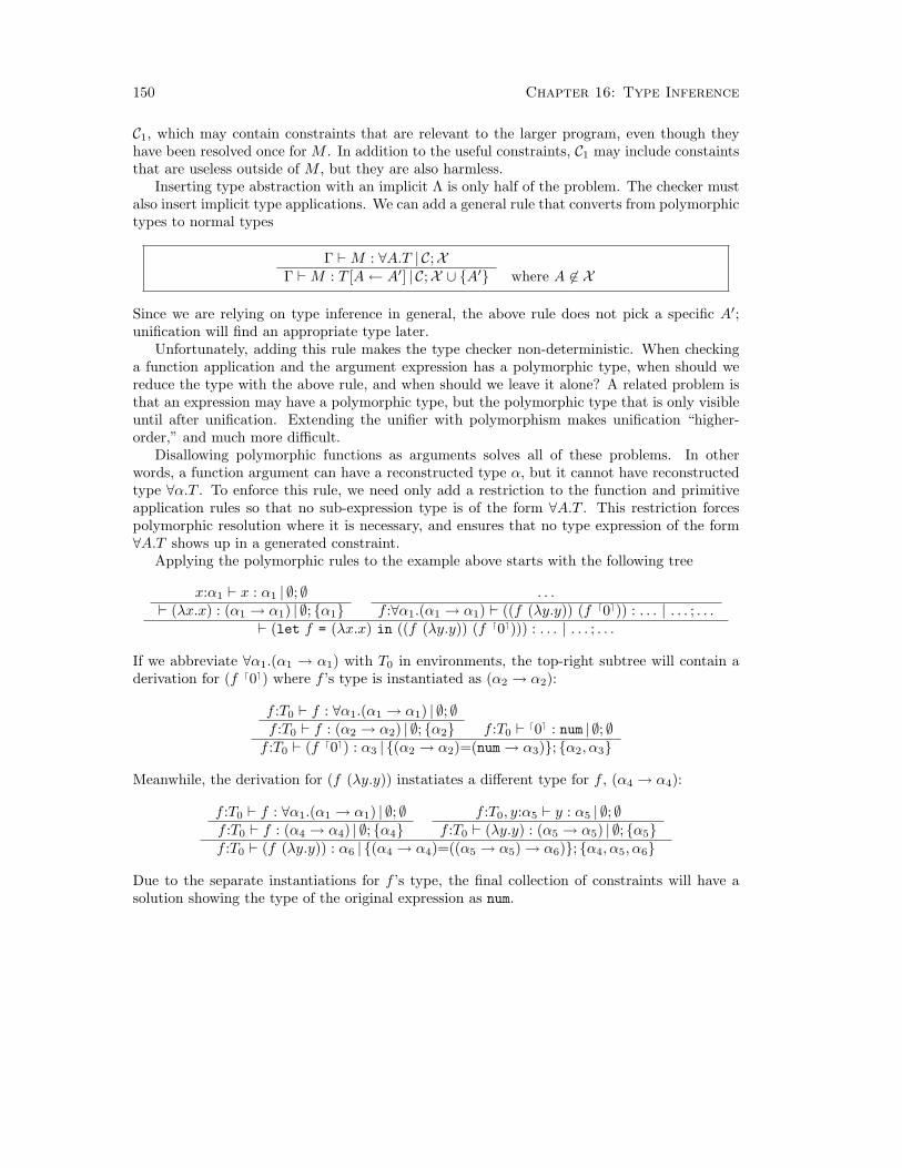
150 Chapter 16: Type Inference
C1, which may contain constraints that are relevant to the larger program, even though theyhave been resolved once for M . In addition to the useful constraints, C1 may include constaintsthat are useless outside of M , but they are also harmless.
Inserting type abstraction with an implicit Λ is only half of the problem. The checker mustalso insert implicit type applications. We can add a general rule that converts from polymorphictypes to normal types
Γ `M : ∀A.T | C;XΓ `M : T [A← A′] | C;X ∪ A′ where A 6∈ X
Since we are relying on type inference in general, the above rule does not pick a specific A′;unification will find an appropriate type later.
Unfortunately, adding this rule makes the type checker non-deterministic. When checkinga function application and the argument expression has a polymorphic type, when should wereduce the type with the above rule, and when should we leave it alone? A related problem isthat an expression may have a polymorphic type, but the polymorphic type that is only visibleuntil after unification. Extending the unifier with polymorphism makes unification “higher-order,” and much more difficult.
Disallowing polymorphic functions as arguments solves all of these problems. In otherwords, a function argument can have a reconstructed type α, but it cannot have reconstructedtype ∀α.T . To enforce this rule, we need only add a restriction to the function and primitiveapplication rules so that no sub-expression type is of the form ∀A.T . This restriction forcespolymorphic resolution where it is necessary, and ensures that no type expression of the form∀A.T shows up in a generated constraint.
Applying the polymorphic rules to the example above starts with the following tree
x:α1 ` x : α1 | ∅; ∅` (λx.x) : (α1 → α1) | ∅; α1
. . .f :∀α1.(α1 → α1) ` ((f (λy.y)) (f d0e)) : . . . | . . . ; . . .
` (let f = (λx.x) in ((f (λy.y)) (f d0e))) : . . . | . . . ; . . .
If we abbreviate ∀α1.(α1 → α1) with T0 in environments, the top-right subtree will contain aderivation for (f d0e) where f ’s type is instantiated as (α2 → α2):
f :T0 ` f : ∀α1.(α1 → α1) | ∅; ∅f :T0 ` f : (α2 → α2) | ∅; α2 f :T0 ` d0e : num | ∅; ∅
f :T0 ` (f d0e) : α3 | (α2 → α2)=(num→ α3); α2, α3
Meanwhile, the derivation for (f (λy.y)) instatiates a different type for f , (α4 → α4):
f :T0 ` f : ∀α1.(α1 → α1) | ∅; ∅f :T0 ` f : (α4 → α4) | ∅; α4
f :T0, y:α5 ` y : α5 | ∅; ∅f :T0 ` (λy.y) : (α5 → α5) | ∅; α5
f :T0 ` (f (λy.y)) : α6 | (α4 → α4)=((α5 → α5)→ α6); α4, α5, α6
Due to the separate instantiations for f ’s type, the final collection of constraints will have asolution showing the type of the original expression as num.

151
Chapter 17: Recursive Types
Throughout our exploration of types so far, we have encountered expressions that could notbe given a type because an equation of the form T1 = . . . T1 . . . could not be solved with aconcrete type for T1. For example, Ω has no type because T1 = (T1 → T2) has no solution forT1. The same problem appears with more useful recursive functions that are written in thestyle of Chapter 4.
As we saw in Chapter 14, we can add fix to the language to support recursive functions, buta programmer still cannot write Ω or λ-calculus-style recursive functions directly. For the samereasons that motivate type inference, we might prefer to type plain ISWIM expressions as muchas possible, including Ω, without forcing a programmer write down type-specific annotations.Inference for general recursive functions requires a way to solve type constraints of the formT1 = . . . T1 . . ..
More importantly, recursive type equations show up in data structures as well as functions.For example, the definition of a list of numbers is inherently recursive:
A list of numbers is either
• null, or
• (cons n l) where n is a number and l is a list of numbers.
We know how to deal with the case split, using disjoint sums, and we can use f for null andpairs for cons. But the second part of the sum type must be a pair type that refers back to theentire sum. In other words, the type Listnum must obey the following equation:
Listnum = (bool + (num× Listnum))
Following Chapter 14, we could solve the problem by building lists directly into the type system.But the more general approach of solving recursive equations is especially valuable to theprogrammer in the case of data, as opposed to functions. A recursive function is a recursivefunction, but a recursive data structure can have many different shapes: a list, a tree, etc.Supporting all possible data shapes in the core type rules requires a general form of recursivetypes. In this chapter, we study recursive types by extending Polymorphic ISWIM (i.e., weignore inference from now on).
17.1 Fixed-points of Type Abstractions
To abstract expressions over types (e.g., to get polymorphic functions), we drew inspirationfrom our expression language, where we could already parameterize expressions over values. Asa result, we added type abstractions (Λα.M) and type applications M [T ] to the grammar ofexpressions, and universal types (∀α.T ) to the grammar of type expressions.
To solve a recursive equation like the one for Listnum, we can similarly draw on our experi-ence with recursive functions: we can add a tfix form for type expressions that takes a typeabstraction and produces it’s fixed point:
Listnum.= tfix (∀α.(bool + (num× α)))
Adding tfix to our type language will work, but by convention, a tfix and its following ∀ arecollapsed together into a single µ:
Listnum.= µα.(bool + (num× α))

152 Chapter 17: Recursive Types
A type constructed with µ is a recursive type. In the same way that f in (fix λf.(λx.(f x))stands for the entire recursive function within (λx.(f x)), the α above stands for the entirerecursive type within (bool + (num× α)).
As another example, consider the expression:
λx.(+ (x x) d5e)
Due to the call (x x), The type of x must be a function type. Since the result of the call isused in an addition expression, the result of the function must be a number. Meanwhile, theargument of the function must have the same type as the function itself. Thus, the type for xabove is
µα.(α→ num)
and the type for the entire function expression is
((µα.(α→ num))→ num)
The type for the function shows how µ can appear embedded within a larger type expression.To support recursive types in general, we extend our grammar for T as follows:
T = . . .| (µA.T )
17.2 Equality Between Recursive Types
One difference between recursive functions and recursive types is that we generally do not needto compare two function values, but type checking requires that we compare type expressionsfor equality. Of course, the type variable bound by a µ type is arbitrary, and we should equatetypes that are simple “α-conversions” of each other, just as we did for ∀ type expressions:
µα.(α→ num) is the same as µβ.(β → num)
But parallels between fix and µ suggest some additional complexities in the comparison process.For example,
(fix λf.(λx.(f x))
andλx.((fix λf.(λx.(f x))) x)
are equivalent expressions, in the sense that they behave the same way in all contexts. Similarly,
µα.(α→ num)
and((µα.(α→ num))→ num)
and(((µα.(α→ num))→ num)→ num)
are all equivalent types, in the sense that an expression having any of these types can be usedas an expression with any of the other types. Type rules therefore require an extended ` ↔relation that captures the equality of types containing µ.
` T [A← A′′]↔ T ′[A′ ← A′′]` (µA.T )↔ (µA′.T ′) where A′′ 6∈ FV(T ) ∪ FV(T ′)
` T [A← (µA.T )]↔ T ′
` (µA.T )↔ T ′` T ′ ↔ T [A← (µA.T )]` T ′ ↔ (µA.T )

17.3 Isomorphisms Between Recursive Types 153
This equivalence relation lets us unfold a type (µA.T ) by replacing each A in T with (µA.T ).Unfolding a recursive type can put it into a form that matches another type.
In addition to extending the type-equivalence relation, the function application rule mustallow a µ type for the first sub-expression, instead of an immediate function type. In otherwords, instead of requiring the function expression to have type (T ′ → T ), it need only producea type that is equivalent to some (T ′ → T ).
Γ `M : T0 ` T0 ↔ (T ′ → T ) Γ ` N : T ′′ ` T ′ ↔ T ′′
Γ ` (M N) : T
We now have two equivalances to prove in the application rule, ` T0 ↔ (T ′ → T ) and ` T ′ ↔T ′′. They can be collapsed into a single rule: ` T0 ↔ (T ′′ → T ):
Γ `M : T0 ` T0 ↔ (T ′′ → T ) Γ ` N : T ′′
Γ ` (M N) : T
Using the new rules, we can assign a type to half of Ωnum, where r abbreviates (µα.(α→ num)):
x:r ` x : r` (r→ num)↔ (r→ num)` r↔ (r→ num) x:r ` x : r
` (λx:r.(x x)) : (r→ num)
To show the type equivalence in the top middle of the tree, we expand the abbreviation r as(µα.(α→ num)), unfold it to ((µα.(α→ num))→ num), and re-abbreviate as (r→ num).
The rules above define a powerful type system for programming with recursive types. Suchrecursive types are call equi-recursive types, because the type rules relate a recursive typeand its unfolded version as equivalent. The main cost of equi-recursive types is that typechecking does not have a straightforward algorithm. When equating recursive types, multiple` ↔ rules can apply, and a winning strategy for building a complete tree is not alwaysapparent. Furthermore, combining recursive types with type inference would aggravate theproblem considerably.
Exercise 17.1. Show that Ωnum, expressed as
(λx:(µα.(α→ num)).(x x)) (λx:(µα.(α→ num)).(x x))
has a type. What if every num is replaced above by an arbitrary type T?
17.3 Isomorphisms Between Recursive Types
An alternative to the powerful equational system required by equi-recursive types is to havethe programmer explicitly specify the places in an expression where recursive types must befolded or unfolded. Such explicit annotations, which generate iso-recursive types, guide typechecking and inference for recursive types in the same way that a let form can guide typeinference for ploymophism.
To support iso-recursive programmer annotations, we must extend the grammar of expres-sions with fold and unfold forms:
M = . . .| (fold M)| (unfold M)

154 Chapter 17: Recursive Types
During evaluation, a fold annotation sticks to a value until it is dismissed by an unfold:
V = . . .| (fold V )
E = . . .| (fold E)| (unfold E)
(unfold (fold V )) f V v = . . . ∪ f
The primary role of fold and unfold is in the type checking rules. We revert the ` ↔relation back to its simple form, from Chapter 15, as well as the function application rule. Allwe need for type checking are two new rules:
Γ `M : T [A← (µA.T )]Γ ` (fold M) : (µA.T )
Γ `M : (µA.T )Γ ` (unfold M) : T [A← (µA.T )]
Using iso-recursive types, a well-typed half of Ωnum requires a strategically placed unfoldannotation:
λx:(µα.(α→ num)).((unfold x) x)
This expression can be typed using the new unfold rule, where r still abbreviates (µα.(α →num)):
x:r ` x : rx:r ` (unfold x) : (r→ num) x:r ` x : r ` r↔ r
` (λx:r.((unfold x) x)) : (r→ num)
Writing all of Ω requires a fold annotation in addition:
(λx:(µα.(α→ num)).((unfold x) x)) (fold λx:(µα.(α→ num)).((unfold x) x))
Exercise 17.2. Show that the representation of Ω above has a type.
17.4 Using Iso-Recursive Types
Iso-recursive types simplify the type checking process, and also work with a straightforwardextension to the type-inference algorithm developed in the preceding chapter.
Realistic programming languages generally do not support recursive types to implementrecursive functions, because fix (or the implicit fix in a let rec form) works well enough.ML, for example, does not support recursive function types, but it provides iso-recursive typesthrough datatype declarations. Nevertheless, ML has no explicit fold and unfold keyword;instead, each use of a constructor to create a value implies a fold, and each use of a constructorin a pattern match implies unfold.
Using recursive and polymorphic types, we can (finally!) define a well-typed, general-purposeimplementation of lists. Our implementation is much like an ML implementation, but withexplcit Λ and fold annotations.
We start with a macro for the type of lists containing elements of type T , and an unfoldedversion of the same type:
ListT.= µα.(bool + (T × α))
UListT.= (bool + (T × ListT ))
We can use this type macro in defining our expression macros. For example, the cons macro willbe a polymorphic function of type ∀α.(α → (Listα → Listα)). Even null must be polymorphic,because the null for different kinds of lists will have a different type.

17.4 Using Iso-Recursive Types 155
What should car and cdr do when they are given null as an argument? Our language currentlyhas no mechanism for signalling errors, and soundness prevents the macros from getting stuck onbad inputs. One sneaky solution is to loop forever, exploting the fact that Ω can be constructedto “return” any type of value (see Exercise 14.4).
null.= Λα.(fold (ToLeftUListα
f))cons
.= Λα.(λv:α.λl:Listα.(fold (ToRightUListα〈v, l〉)))
car.= Λα.(λl:Listα.(Match(UListα→α) (unfold l)
(λn:bool.Ω[α])(λp:(α× Listα).(fst p))))
cdr.= Λα.(λl:Listα.(Match(UListα→Listα) (unfold l)
(λn:bool.Ω[Listα])(λp:(α× Listα).(snd p))))
isnull.= Λα.(λl:Listα.(Match(UListα→bool) (unfold l)
(λn:bool.t)(λp:(α× Listα).f)))
Ω .= Λα.( (λx:(µβ.(β → α)).((unfold x) x))(fold λx:(µβ.(β → α)).((unfold x) x)) )
The null and cons macros act like ML type constructors, and as expected, they each contain afold form. Similarly, the car, cdr, and isnull macros act like deconstructing pattern matches,so each uses unfold on its argument.
Exercise 17.3. Show that
(car[num] (cons[num] d1e null[num]))
reduces to d1e, and show that it has type num. To simplify the type derivation, assume that wehave already shown Γ ` Ω[T ] : T for all Γ and T .

156 Chapter 17: Recursive Types

157
Chapter 18: Data Abstraction and Existential Types
Type soundness ensures that applications of primitive operations do not “go wrong” in the sensethat primitive operations are never applied to bad arguments. The information that a programcannot go wrong is perhaps most useful to a programmer, but language implementors can alsoput that information to work. For example, zero and false can be represented in the sameway, without the possibility of strange behavior when false is added to a number. Similarly,functions can be represented by memory addresses, without the possibility that a number willbe mis-used as the address of a non-existent function.
In other words, types can hide some of the implementation details of a language. The powerto hide implementation details can be useful to programmers, as well as language implementors,particularly for building modularized software. For example, given our implementation of nulland cons from the previous chapter, we’d prefer that client programmers using cons always usecar to extract the first element of a list, so that we can change the implementation of cons later ifbecomes necessary. Such good programming style is not enforced by the type language, however,at least not for the way we wrote the code in the previous chapter. The type ListT is merelyan abbreviation, and completely transparent to client programmers. Using the expanded type,a client programmer can manipulate list internals directly, either intentionally or accidentally.
To hide the details of the list type from the programmer, we can force client programmersto implement list-using code in a particular way: client code must have the type ∀α.T for someT , where α serves as the type for lists. Since the client code is polymorphic with respect to listvalues, the client cannot rely on any implementation details about lists.
This approach to data abstraction can codified through a specific extension of the pro-gramming language: existential types. Like a universal type ∀A.T , an existential type ∃A.Tdescribes a value that works with arguments of an unspecified type A. In the case of a univer-sial type, the unspecified type can be replaced by any type. In the case of an existential type,the unspecified type can be replaced by only one particular type. That one particular type ishidden from client programmers, and the type system can enforce the hiding. As well will see,the difference between ∀A.T and ∃A.T is essentially two levels of procedure indirection.
18.1 Data Abstraction in Clients
Lists are one example of a datatype that we might like to keep abstract from clients, butour current implementation of lists is perhaps the only one that makes sense. For an examplewhere different implemenations of the abstract type could make sense, suppose that a particularprogram requires a few numbers that are known at start-up, uses the numbers repeatedly inaddition expressions, and then requires a fast odd/even parity test. In this case, the abstractdatatype is the type of parity-testable numbers, and an implementation of the datatype willprovide functions for construction the initial numbers, adding numbers, and checking the parityof a number.
If the base language provides numbers and bitwise operators, the parity test is trivial. Thus,one implementation of the datatype exploits a fast isodd function that is built into the languageimplementation:
Num1.= num
mknum1.= λn:num.n
add1.= λn:Num1.λm:Num1.(+ n m)
parity1.= λn:Num1.(isodd n)
nfuncs1.= 〈mknum1, 〈add1, parity1〉〉

158 Chapter 18: Data Abstraction and Existential Types
The nfuncs1 tuple bundles the number operations into a tuple that acts like a “library module”to be supplied to client programmers.
If the base language does not provide bitwise operators (or other operators that can be usedto test for even and odd), then we can optimize the parity test by computing the parity ofthe initial numbers, tracking parity during additions, and then extracting the parity value ofthe result. Thus, a second implementation of the datatype uses (num × bool) to implementparity-maintained numbers:
Num2.= (num× bool)
mknum2.= λn:num.〈n, (isodd n)〉
add2.= λn:Num2.λm:Num2.〈(+ (fst n) (fst m)), (xor (snd n) (snd m))〉
parity2.= λn:Num2.(snd n)
nfuncs2.= 〈mknum2, 〈add2, parity2〉〉
where isodd and xor are defined in the obvious way. (The isodd function will require O(n) timefor an integer n, while xor is constant time.)
Each module-like tuple nfuncsi has type NFuncsNumiwhere
NFuncsT.= ((num→ T )× ((T → (T → T ))× (T → bool)))
Instead of supplying the tuple nfuncs1 or nfuncs2 directly to clients, we can hide the specificimplementation type Numi by requiring clients to have the form
∀α.(NFuncsα → T )
In other words, client code must be represented by a polymorphic function that cannot rely onthe details of the number type α. The function consumes a tuple representing the number op-erations. The body of the function corresponds to the client code proper; it uses the operationsto produce some value of type T .
For example, here is a client that adds 17 and 18, then extracts the parity of the result:
client.= Λα.λn:NFuncsα (let m:(num→ α) = (fst n)
a:(α→ (α→ α)) = (fst (snd n))p:(α→ bool) = (snd (snd n))
in (p (a (m d17e) (m d18e)))))
where the multiple-variable let macro has the obvious expansion. It extracts the functions ofthe “imported module” tuple n into the local variables m, a, and p.
To execute client, we must apply it to one of the implemenations of numbers, either
(client[Num1] pfunctions1)
or(client[Num2] pfunctions2)
The type system ensures that both applications will work, as long as client has the ∀α . . . typeabove (for some specific T ).
18.2 Libraries that Enforce Abstraction
Our goal is to forcing clients to respect data abstraction, but the enforcement is backward.In practice, it is the library implementor who should enforce generality, and not the linkingprogrammer, so that the library implementor is free to implement a library in different ways.

18.3 Existential ISWIM 159
If a library implementor provided nfuncs1 or nfuncs2 directly to other programmers, the otherprogrammers could rely on the type Num1 or Num2 directly, conflicting with a future revisionof the library that changes the implementation type for numbers.
This problem is easily corrected by supplying to programmers a library as a linking proce-dure, instead of as a tuple. In other words, the library provided by a programmer will combinenfuncs1 or nfuncs2 with the linking application:
ClientT.= ∀α.(NFuncsα → T )
nlib1.= Λβ.λc:Clientβ .(c[Num1] pfunctions1)
nlib2.= Λβ.λc:Clientβ .(c[Num2] pfunctions2)
Note that nlib1 and nlib2 must be parameterized by β, which is the return type of the clientusing the library. Given nlib1 or nlib2, we can link the client program with
(nlib1[bool] client)
or(nlib2[bool] client)
The only difference from before is that, given only pfunctioni instead of nfuncsi, the linkingprogrammer cannot abuse the library by linking it to a client that exploits the concrete type ofnumbers. In other words, the type on the c argument of pfunctioni forces clients to respect thedata abstraction.
18.3 Existential ISWIM
The nlib1 and nlib2 functions each consume a polymorphic function as an argument. Althoughthis is not a problem in principle, we saw in Section 16.2 that polymorphic values introduceproblems for type inference, and are thus disallowed in some languages. We can support module-like packages without polymorphic values by adjusting our language to turn the abstraction-enforcing function “inside out.”
The idea is to capture just the core part of nlib1 and nlib2. The type of both expressions is∀β.(∀α.(NFuncsα → β)→ β). The β parts really have nothing to do with the library, only theclients; mentioning those polymorphic clients requires polymorphic values, which is the part wewant to eliminate. To pull out the NFuncsα path, we need a way to lift the function arrow outof the ∀α... type. To support such lifting, we will enrich our language with existential types.
Using our new extensions, the type of the library expression will be
∃α.NFuncsα
which means “a tuple of three functions involving α, for some hidden type α”. Just as ∀ typesrequire a creation form (ΛA.M) and an application form M [T ], ∃ types require a creation anduse form. The creation form is pack:
(pack[A=T ] M as T ′)
where M generates the value whose reprsentation is to be partially hidden. The variable A willrepresent the hidden type, T is the actual hidden type, and T ′ is the type of M where someinstances of T have been replaced by A. The type of the overall pack expression will be ∃A.T ′.
For example, we can use pack to create our two implementations of numbers as follows:
npack1.= (pack[α=Num1] nfuncs1 as NFuncsα)
npack2.= (pack[α=Num2] nfuncs2 as NFuncsα)

160 Chapter 18: Data Abstraction and Existential Types
The type of both expressions is the existiential type we wanted, ∃α.NFuncsα, which in expandedform is ∃α.((num→ α)× ((α→ (α→ α))× (α→ bool))).
The unpack form uses an abstraction created by pack. While unpacking, it does not exposethe implementation type hidden by pack, but instead declares a local type name to stand forthe hidden type, much like the Λ-bound variable stood for the hidden type in the old encoding:
(unpack[A] X from M in M ′)
where M ′ produces a packed value, the variable A stands for the hidden type locally, thevariable X recieves the unpacked value produced by M , and the body M ′ uses the unpackedvalue polymorphically in A.
For example, to use npack1, we select a variable γ to stand in place of the unknown type inclient code:
(unpack[γ] n from npack1 in(let m:(num→ γ) = (fst n)
a:(γ → (γ → γ)) = (fst (snd n))p:(γ → bool) = (snd (snd n))
in (p (a (m 17) (m 18)))))
Since npack1 has type ∃α.((num → α) × ((α → (α → α)) × (α → bool))), the unpack[γ]expression causes n to have the type ((num → γ) × ((γ → (γ → γ)) × (γ → bool))), which isconsistent with the let bindings. The overall program therefore has type bool.
Note that the body of the unpack expression cannot exploit the concrete representation ofnumbers hidden by pack, because the type is reduced to simply γ. Furthermore, if we try tomix functions from the two packages, as in the following expression, the resulting program hasno type, because γ1 6= γ2 (i.e., no two type variables are ever known to be equal):
(unpack[γ1] n1 from nlib1 in(unpack[γ2] n2 from nlib2 in
(let m1:(num→ γ1) = (fst n1)a1:(γ1 → (γ1 → γ1)) = (fst (snd n1))p2:(γ2 → bool) = (snd (snd n2))
in (p2 (a1 (m1 17) (m1 18))))))
Using γ1 for both unpack expressions would not allow the packages to be confused, either. Theγ1s would be different in the same sense that the xs in (λx.λx.x) are different.
Hiding implies that a value of type ∃α.(α → bool) is by itself useless; since the typeα is unknown, the function cannot be applied to any value. In contrast, a value of type∃α.((num→ α)× (α→ bool)) can be useful. The first function in the pair can construct valuesof type α, and the second function in the pair can consume those values. The programmerusing such a value need not know anything about the implementation of intermediate value oftype α.
To add existential types to ISWIM to form Existential ISWIM, we extend the expressiongrammar with pack and unpack forms, where the pack form generates values.
M = . . .| (pack[A=T ] M as T )| (unpack[A] X from M in M)
T = . . .| (∃A.T )
V = . . .| (pack[A=T ] V as T )
E = . . .| (pack[A=T ] E as T )| (unpack[A] X from E in M)
(unpack[A] X from (pack[A′=T ′] V as T ) in M) x M [X ← V ][A← T ′]
v = . . . ∪ x
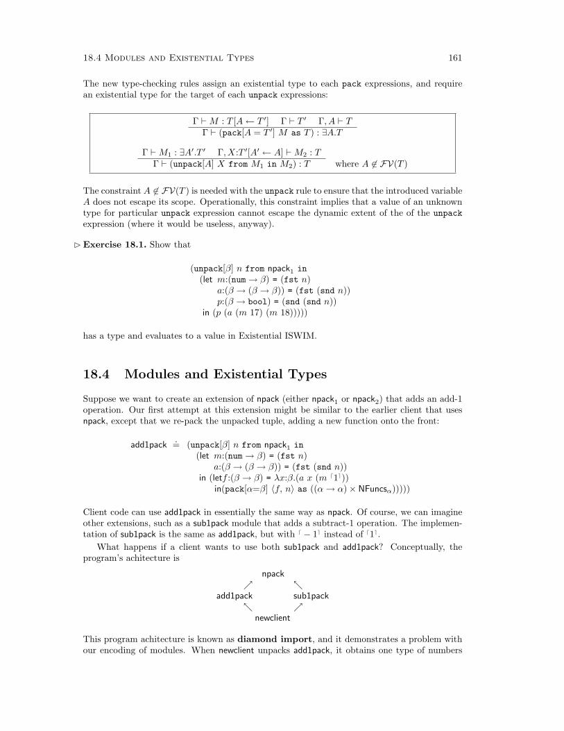
18.4 Modules and Existential Types 161
The new type-checking rules assign an existential type to each pack expressions, and requirean existential type for the target of each unpack expressions:
Γ `M : T [A← T ′] Γ ` T ′ Γ, A ` TΓ ` (pack[A = T ′] M as T ) : ∃A.T
Γ `M1 : ∃A′.T ′ Γ, X:T ′[A′ ← A] `M2 : TΓ ` (unpack[A] X from M1 in M2) : T where A 6∈ FV(T )
The constraint A 6∈ FV(T ) is needed with the unpack rule to ensure that the introduced variableA does not escape its scope. Operationally, this constraint implies that a value of an unknowntype for particular unpack expression cannot escape the dynamic extent of the of the unpackexpression (where it would be useless, anyway).
Exercise 18.1. Show that
(unpack[β] n from npack1 in(let m:(num→ β) = (fst n)
a:(β → (β → β)) = (fst (snd n))p:(β → bool) = (snd (snd n))
in (p (a (m 17) (m 18)))))
has a type and evaluates to a value in Existential ISWIM.
18.4 Modules and Existential Types
Suppose we want to create an extension of npack (either npack1 or npack2) that adds an add-1operation. Our first attempt at this extension might be similar to the earlier client that usesnpack, except that we re-pack the unpacked tuple, adding a new function onto the front:
add1pack.= (unpack[β] n from npack1 in
(let m:(num→ β) = (fst n)a:(β → (β → β)) = (fst (snd n))
in (letf :(β → β) = λx:β.(a x (m d1e))in(pack[α=β] 〈f, n〉 as ((α→ α)× NFuncsα)))))
Client code can use add1pack in essentially the same way as npack. Of course, we can imagineother extensions, such as a sub1pack module that adds a subtract-1 operation. The implemen-tation of sub1pack is the same as add1pack, but with d − 1e instead of d1e.
What happens if a client wants to use both sub1pack and add1pack? Conceptually, theprogram’s achitecture is
npack
add1pack sub1pack
newclient
This program achitecture is known as diamond import, and it demonstrates a problem withour encoding of modules. When newclient unpacks add1pack, it obtains one type of numbers

162 Chapter 18: Data Abstraction and Existential Types
γ1, and when newclient unpacks add1pack, it obtains another type of numbers γ2:
(unpack[γ1] n1 from add1pack1 in(unpack[γ2] n2 from sub1pack2 in
(let m1:(num→ γ1) = (fst (fst n1))a1:(γ1 → γ1) = (fst n1)s2:(γ2 → γ2) = (fst n2)
in (s2 (a1 (m1d0e))))))
This expression has no type, because the result of a call to the add-1 function cannot beprovided to the sub-1 function; the types are not compatible. Actually, the representations arecompatible, and the evaluation of (s2 (a1 (m1
d0e))) would not get stuck, but the type systemis enforcing too many abstraction boundaries.
We can adjust our encoding of modules to solve this problem. The source of the problem isthat add1pack and sub1pack each separately unpack the original npack. To avoid this unpacking,we can return to our earlier use of explicit Λ for “clients”, though in this case the two clients serveas libraries to other clients. Another part of the problem is that both add1pack and sub1packre-pack the content of the original npack. In our revised encoding, we will assume instead thatclients of add1pack and sub1pack explicitly import npack to get the base funtionality.
Putting the pieces together, our new definition follows:
add1module.= Λβ.λn:NFuncsβ .
(let m:(num→ β) = (fst n)a:(β → (β → β)) = (fst (snd n))
in (letf :(β → β) = λx:β.(a x (m d1e))in f)))
The definition of sub1module is similar. The body of the module is simply f because add1moduleand sub1module do not introduce any new abstract types. The body of a module that doesintroduce a new abstract type would have the form (pack[α=T ] M as (β → β)) for some hiddentype T .
In general, the type of a module will have the shape
∀β . . . λx:Tβ....∃α . . . Tα...,β...
where a sequence of βs represents the imported abstract types, the type Tβ... corresponds tomodule imports whose types mention the βs, a sequence of αs represents exported abstracttypes, and the type Tα...,β... corresponds to a set of exports whose types mention the αs andβs.
To use add1module and sub1module, a client must link them together with npack:
(unpack[γ] n from npack1 in(let a = (add1module[γ] n)in (let s = (sub1module[γ] n)
in (let m:(num→ γ1) = (fst n)in (s2 (a1 (m1
d0e)))))))
The main drawback of this approach is readily apparent. As the number of modules thatcomprise a program grows, and as modules become more interconnected, the client programmeris responsible for an increasingly complex linking step to assemble the program. In practice,this problem can be tempered by staging the linking steps; linking must be delayed only wherediamond imports occur, but completed diamonds can be sealed. But when a library module isused through a large program, it tends to generate diamonds that are resolved only in the finallinking steps.
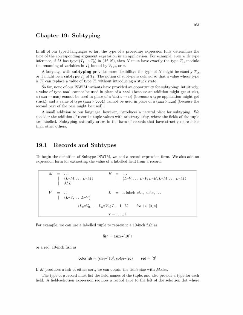
163
Chapter 19: Subtyping
In all of our typed languages so far, the type of a procedure expression fully determines thetype of the corresponding argument expression in an application. For example, even with typeinference, if M has type (T1 → T2) in (M N), then N must have exactly the type T1, modulothe renaming of variables in T1 bound by ∀, µ, or ∃.
A language with subtyping provides more flexibility: the type of N might be exactly T1,or it might be a subtype T ′1 of T1. The notion of subtype is defined so that a value whose typeis T ′1 can replace a value of type T1 without introducing a stuck state.
So far, none of our ISWIM variants have provided an opportunity for subtyping: intuitively,a value of type bool cannot be used in place of a bool (because an addition might get stuck),a (num→ num) cannot be used in place of a ∀α.(α→ α) (because a type application might getstuck), and a value of type (num× bool) cannot be used in place of a (num× num) (because thesecond part of the pair might be used).
A small addition to our language, however, introduces a natural place for subtyping. Weconsider the addition of records: tuple values with arbitrary arity, where the fields of the tupleare labelled. Subtyping naturally arises in the form of records that have structly more fieldsthan other others.
19.1 Records and Subtypes
To begin the definition of Subtype ISWIM, we add a record expression form. We also add anexpression form for extracting the value of a labelled field from a record:
M = . . .| 〈L=M, . . . L=M〉| M.L
V = . . .| 〈L=V, . . . L=V 〉
E = . . .| 〈L=V, . . . L=V,L=E,L=M, . . . L=M〉
L = a label: size, color, . . .
〈L0=V0, . . . Ln=Vn〉.Li l Vi for i ∈ [0, n]
v = . . . ∪ l
For example, we can use a labelled tuple to represent a 10-inch fish as
fish.= 〈size=d10e〉
or a red, 10-inch fish as
colorfish.= 〈size=d10e, color=red〉 red
.= d3e
If M produces a fish of either sort, we can obtain the fish’s size with M.size.The type of a record must list the field names of the tuple, and also provide a type for each
field. A field-selection expression requires a record type to the left of the selection dot where

164 Chapter 19: Subtyping
the field to the right of the dot is included in the record:
T = . . .| 〈L:T, . . . L:T 〉
Γ `M0 : T0 . . . Γ `Mn : Tn
Γ ` 〈L0=M0, . . . Ln=Mn〉 : 〈L0:T0, . . . Ln:Tn〉
Γ `M : 〈L0:T0, . . . Ln:Tn〉Γ `M.Li : Ti where i ∈ [0, n]
For example, the type of fish is 〈size:num〉 and the type of colorfish is 〈size:num, color:num〉.Using a record type for a function argument, we can define a function that takes a fish and
returns its size:fsize
.= λf :〈size:num〉.f.sizeThis function has type (〈size:num〉 → num). Naturally, the expression (fsize fish) has type num,and it produces the value d10e when evaluated.
What about (fsize colorfish)? When evaluated, it also produces d10e. But this expressionhas no type, because fsize consumes an argument of type 〈size:num〉, while colorfish has type〈size:num, color:num〉. Clearly, we want to make 〈size:num, color:num〉 a subtype of 〈size:num〉,because (intuitively) replacing fish with colorfish can never cause a program to become stuck.
In general, any record type that has at least the fields of another record type should be asubtype. To define subtypes formally, we introduce a ≤ relation, where T ≤ T ′ means “T is asubtype of T ′.” Initially, we define the relation as follows:
T ≤ T
〈L0:T0, . . . Ln:Tn〉 ≤ 〈L′0:T ′0, . . . L′m:T ′m〉if L0:T0, . . . Ln:Tn ⊇ L′0:T ′0, . . . L′m:T ′m
The notation ≤ suggests the following intuition about the meaning of subtyping: the set ofvalues belonging to a subtype is smaller than the set of values belonging to the original type,because the latter includes the former.
We also adjust the rule for function application to allow subtypes in the argument position:
Γ `M : (T ′ → T ) Γ ` N : T ′′ T ′′ ≤ T ′
Γ ` (M N) : T
(To correctly handle polymorphism and recursive types, we could adjust our subtyping rule toabsorb the ` ↔ relation, but we ignore the extra complexity.)
Using the new rules, we can show a type for (fsize colorfish), abbreviating num with n, sizewith s, and color with c:
f :〈s:n〉 ` f : 〈s:n〉f :〈s:n〉 ` f.s : n
` (λf :〈s:n〉.f.s) : (〈s:n〉 → n) ` 〈s=d10e, c=red〉 : 〈s:n, c:n〉 〈s:n, c:n〉 ≤ 〈s:n〉` ((λf :〈s:n〉.f.s) 〈s=d10e, c=red〉) : n
Exercise 19.1. Does(if M fish colorfish).size
produce a value when evaluated, assuming that M produces either t or f? Does it have a typeusing our rules so far, assuming `M : bool? If not, should it? If not, and if it should, suggesta sound revision to a type rule so that the expression has a type.

165
19.2 Subtypes and Functions
Our revised type rules not only give (fsize colorfish) a type, but we can apply any function onfishes to color fishes. Indeed, we can write a function that takes an arbitrary function on fishesand applies it to colorfish:
apply.= λf :(〈size:num〉 → num).(f colorfish)
We can easily verify that (apply fsize) has a type. Suppose that we have a function that extractsa fish’s color:
cfcolor.= λf :〈size:num, color:num〉.f.color
Can we use cfcolor as an argument to apply? According to the type system, the answer is “no”,even though (apply cfcolor) produces a value.
In this case, the type system’s restriction is justified. The body of apply would be well-typedif the argument of f is changed to fish instead of colorfish. If we made that change and thenapplied apply to cfcolor, evaluation would get stuck.
If we really want to apply functions to colorfish, then we should declare a different type onthe argument of apply:
capply.= λf :(〈size:num, color:num〉 → num).(f colorfish)
Again, we can easily verify that (capply cfcolor) has a type. But now (capply fsize) has no type,although it still produces a value.
In this case, the type system is too restrictive. Since every function on fishes works on colorfishes, capply should accept both kinds of functions. There is no one type we can write forcapply’s argument, but we can extend our subtyping relation. Again, every function on fishesworks on color fishes, which means that the type of a function on fishes should be a subtype ofa function on colorfishes:
(〈size:num〉 → num) ≤ (〈size:num, color:num〉 → num)
At first glance, this relation may look backward, but it is not. Intuitively, a color fish is aspecial kind of fish, but a function on fishes is a special kind of function on color fishes. Putanother way, the set of fishes is larger than the set of color fishes (because the former includesthe latter), and the set of functions that work on color fishes is larger than the set of functionsthat work on fishes (because the former includes the latter).
In general, a subtype relation for the argument part of a function type induces the reverserelation on the function type as a whole. A position in type expression with this property iscalled a contra-variant position.
Before we define the general subtyping rule on function types, consider the result position.Suppose a function returns a color fish; can it be used in place of a function that returns a fish?Yes, just as a color fish can be used in place of a fish. This less surprising kind of position iscalled co-variant: a subtype relation in the result position of a function type induces the samesubtype relation in the function type as a whole.
Thus, the general rule for function subtyping is as follows:
T ′1 ≤ T1 T2 ≤ T ′2(T1 → T2) ≤ (T ′1 → T ′2)
Using this new rule, we can show a type for (capply fsize):
. . .` capply : ((〈s:n, c:n〉 → n)→ n)
· · ·` fsize : (〈s:n〉 → n)
〈s:n, c:n〉 ≤ 〈s:n〉 n ≤ n(〈s:n〉 → n) ≤ (〈s:n, c:n〉 → n)
` (capply fsize) : n

166 Chapter 19: Subtyping
19.3 Subtypes and Fields
Suppose that we define a type for a two-fish school:
School.= 〈one:〈size:num〉, two:〈size:num〉〉
Should we be able to use a school composing two color fish as a school of plain fish?
cschool.= 〈one=〈size:1, color:red〉, two=〈size:1, color:blue〉〉
Yes. A school of color fish clearly works wherever a school of fish works, because the onlypossible operation on a school is to extract its fish, and the fish are individually replaceablewith color fish.
More generally, we can allow subtypes on fields within records co-variantly.
〈L0:T0, . . . Ln:Tn〉 ≤ 〈L′0:T ′0, . . . L′m:T ′m〉if L0, . . . Ln ⊇ L′0, . . . L′mand (Li = L′j)⇒ (T ′i ≤ Tj) for i ∈ [0, n], j ∈ [0,m]
As it turns out, few realistic programming languages support this kind of subtyping. The reasonis that such languages tend to provide an additional operation on records: field update. Whenfield update is allowed along with subtyping on record fields, a field might get replaced with asupertype value. For example, a color school might be used as a plain school, and then the onefield of the school could be updated with a fish (not a color fish). Other parts of the programthat expect a color school will then find a plain fish in the school, and probably get stuck as aresult.
To support update operations, record fields in a typical language are invariant, whichmeans that they are neither co-variant nor contra-variant. In particular fields of an object inJava are invariant, as we will see in the next chapter.
19.4 From Records to Objects
Objects in an object-oriented language are similar to records. In addition to field values,however, an object encapsulates a set of methods. In a language like ISWIM with procedurevalues, we can encode methods as procedure-valued fields in a record. A procedure representinga method must consume the “self” object as its argument.
Thus, a fish object with a size field and getsize method would be encoded as
fishobj.= 〈size=d10e, getsize=λs:〈size:num〉.s.size〉
To call the getsize “method” of fishobj, we extract the getsize procedure from fishobj and applyit to fishobj:
(fishobj.getsize fishobj)
This expression has a type and produces the expected result.A more realistic encoding of objects requires a more precise type for the argument to getsize.
In particular, methods must be mentioned in the type of s so that the body of the method cancall the object’s own methods—including the getsize method. Such a refinement is possiblewith recursive types, but we ignore this generalization, because we encounter a problem evenwith the simple encoding.
To see the problem, consider a color fish with a getsize method where the fish’s colormultiplies its apparent size:
colorfishobj.= 〈size=d10e, color=d2e, getsize=λs:〈size:num, color:num〉.(∗ s.size s.color)〉

167
Again, the expression for calling getsize of colorfishobj has a type and value:
(colorfishobj.getsize colorfishobj)
But is the type of colorfishobj a subtype of the type for fishobj?Even if we allow co-variant record fields, it is not, because the type of colorfishobj’s getsize
method is not a subtype of the type for fishobj’s getsize method (due to the contra-variance offunction arguments). Indeed, we can see that an expression such as
(colorfishobj.getsize fishobj)
should not have a type, because it will get stuck; fishobj will not have the color field that getsizewants.
The final example not only shows that the encoding should fail, but it shows why: a pro-grammer can construct bad “method calls” where the wrong self object is supplied to themethod. Following our earlier strategy for addressing type problems, we can solve this one bytreating methods differently than fields, and by not allowing method-as-field accesses exceptthose that fit the right pattern. We explore this path in the next chapter.

168 Chapter 19: Subtyping

169
Chapter 20: Objects and Classes
In an untyped setting, we can easily model classes and objects by using λ to construct methodsand pairs or records to construct objects. However, as we saw in the previous chapter, suchan encoding of objects does not work well with the type system of Simply Typed ISWIM orits variants. In the same way that adding pairs to Simply Typed ISWIM was the simplest wayof obtaining well-typed pairs, adding classes and objects to the language—or starting with anentirely new language based on classes—is the simplest and usually most useful way of obtainingwell-typed objects.
In this chapter, we abandon ISWIM and model directly an object-oriented language. Inparticular, we model a subset of the JavaTM language. Java itself is far too large to modelformally in the space of a modest textbook. We choose a subset that contains the programmingelements we are most interested in, which in this case include classes, objects, fields, methods,inheritance, overriding, and imperative field update. We ignore interfaces, abstract methods,exceptions, and arrays.
20.1 MiniJava Syntax
MiniJava is a simplification of Java for studying classes and mutable objects. A MiniJavaprogram is a sequence of class declarations followed by an expression to evaluate (instead ofrelying on a main method). Each class contains a sequence of field declarations (with a typeand constant initial value for each field) followed by a sequence of method declarations.
P = c . . . c M a program
c = class c extends c f . . . f m . . . m class declarationf = T f = V field declarationm = T m(T X, . . . T X) M method declaration
c = a class name or Objectf = a field namem = a method nameX = a variable name or this
The only expression forms are field access, field update, method calls, super calls, and casts.
M = X| null| new c| M :c.f field access| M :c.f := M field assignment| M.m(M, . . .M) method call| super X:c.m(M, . . .M) super call| (c)M cast| b| (on M . . . M)
T = c| B
b = a basic constanton = an n-ary primitive operationB = a basic type

170 Chapter 20: Objects and Classes
In the case of field accesses and updates, the field name is annotated with its source class, sothat we can ignore the problem of field hiding in derived classes. Similarly, for super calls, thetarget object as a variable (usually this) and the superclass are named explicitly. Instead ofmodeling object constructors, every field in an object is initialized to a given constant, whichmust be null for class-typed fields. As usual, we assume an unspecified set of basic constantsb, primitive operations on, and basic types B. The set of types T includes basic types and classnames.
The following example program defines a fish class and a derived colorfish class, and theninstantiates both classes:
class fish extends Object num size = d1e
num getWeight() this:fish.size num grow(num a) this:fish.size := (+ a this:fish.size) num eat(fish f) this.grow(f.getWeight())
class colorfish extends fish
num color = d7e
num getWeight() (∗ super this:fish.getWeight() this:colorfish.color) new fish.eat(new colorfish)
The fish class contains the field size and the methods getWeight, grow, and eat. The getWeightmethod returns the value of the size field in this. The grow method increments the size fieldof this, and the eat method calls grow with the weight of the given fish. The colorfish classadds a color field, and overrides the getWeight method. The overriding declaration chains tofish’s getWeight and multiplies the result by the fish’s color.
A well-formed MiniJava program must obey certain high-level constraints: every class namemust be declared only once, the built-in class Object must not be declared, the fields of eachclass must be unique, the methods of each class must be unique, and every class that is usedmust be declared. These properties are most easily captured by relations defined with “isin”, which relates arbitrary symbol sequences, and with “· · ·”, which stands for an arbitrarysequence of symbols with balanced braces and parentheses.
ClassesOnce(P ) iff(class c · · · class c′ is in P ) implies c 6= c′
ObjectBuiltin(P ) iffclass Object is not in P
FieldsOncePerClass(P ) iff(class c extends c′ · · · T1 f1 · · · T1 f2 · · · is in P ) implies f1 6= f2
MethodsOncePerClass(P ) iff(class c extends c′ · · · T1 m1 · · · T1 m2 · · · is in P ) implies m1 6= m2
ClassesDefined(P ) iff(c is in P ) implies c = Object or (class c is in P )
By inspecting the fish example, we can easily see that all of these relations hold for the exampleprogram.
Besides these basic checks, the declared class must form an inheritance tree (as opposed toa cyclic inheritance graph!), overriding method declarations must be consistent with superclassmethod definitions, and so on.
We can simplify the checking of such properties by defining a few more derived relations

20.1 MiniJava Syntax 171
with “is in”. For example, ≺P relates a class and its declared superclass in P .
c ≺P c′ iffclass c extends c′ is in P
〈c.f, T, V 〉 ∈∈fP c iff
class c extends c′ · · · T f = V · · · is in P
〈m, (T1 . . . Tn → T0), (X1, . . . Xn),M〉 ∈∈mP c iff
class c extends c′ · · · T0 m(T1 X1, . . . Tn Xn) M · · · is in P
In the earlier example, fish ≺P Object, colorfish ≺P fish, 〈colorfish.color, num, d7e〉 ∈∈fP colorfish,
and 〈grow, (num→ num), (a), (+ a this:fish.size)〉 ∈∈mP fish.
The transitive closure of the ≺P relation is the complete subclass relation ≤P , which must beantisymmetric so that inheritance is well-defined (i.e., the subclass relationship among classesmust form a tree):
≤P = transitive–reflexive closure of ≺P
WellFoundedClasses(P ) iff ≤P is antisymmetirc
Using the ≤P relation, we can define the final field-inclusion relation, where a class inherits thefields of its superclass, and also check that method overriding preserves the type of a method.
〈c.f, T, V 〉 ∈fP c′ iff
〈c.f, T, V 〉 ∈∈fP c and c′ ≤P c
OverridesConsistent(P ) iff(〈m, (T1 . . . Tn → T0), (X1, . . . Xn),M〉 ∈∈m
P c1)and (〈m, (T ′1 . . . T ′n → T ′0), (X
′1, . . . X
′n),M ′〉 ∈∈m
P c2)implies (c1 6≤P c2 or (T1 . . . Tn → T0) = (T ′1 . . . T ′n → T ′0))
Thus, 〈fish.size, num, d1e〉 ∈fP fish and 〈fish.size, num, d1e〉 ∈f
P colorfish.For the purposes of type checking, we could define a method-inclusion relation like the one
for fields:〈m, (T1 . . . Tn → T0), (X1, . . . Xn),M〉 ∈m
P c′ iff〈m, (T1 . . . Tn → T0), (X1, . . . Xn),M〉 ∈∈m
P c and c′ ≤P c
However, in the case that a method is overriden, this definition assigns multiple method imple-mentations to a given class for the method name. A more useful relation would pick the mostoverriding implementation of the method, i.e., the one from the minimum class (according tothe ≤P relation) that defines the method.
〈m, (T1 . . . Tn → T0), (X1, . . . Xn),M〉 ∈mP c′ iff
〈m, (T1 . . . Tn → T0), (X1, . . . Xn),M〉 ∈∈mP c
and c = minc | c′ ≤P c and 〈m, (T ′1 . . . T ′n → T ′0), (X′1, . . . X
′n),M ′〉 ∈∈m
P c
For getWeight in fish, we can see that
〈getWeight, (→ num), (), this:fish.size〉 ∈mP fish
but for getWeight in colorfish, we have
〈getWeight, (→ num), (), (∗ super this:fish.getWeight() this:colorfish.color)〉 ∈mP colorfish

172 Chapter 20: Objects and Classes
20.2 MiniJava Evaluation
Since MiniJava provides mutable objects, the evaluation of MiniJava programs requires a store,as in Chapter 11. But unlike mutable variables in ISWIM, the mutable elements in MiniJava areobjects, which can be used as values. Consequently, we not only add σ to the set of MiniJavaexpressions, but also to the set of values. Basic constants, null, and objects (represented bystore addresses) are the only kind of values. To add σ as an expression, it turns out to beconvenient to treat σs as variables. We define also the set of evaluation contexts.
X = a variable name, this, or σ V = b| null| σ
E = [ ]| E:c.f| E:c.f := M| V :c.f := E| E.m(M, . . .M)| V.m(V, . . . V, E,M, . . .M)| super V :c.m(V, . . . V, E,M, . . .M)| (c)E| (on V . . . V E M . . . M)
An object in the store 〈T,FS〉 consists of a class tag T , which indicates the class instantiatedby the object, and a mapping FS from class-prefixed field names to values. The class tag isneeded for method dispatch and for casts.
The tag is only meaningful in the context of the program P ; the evaluation rules combine thetag with static information derived from P . In addition, the program P determines the fieldsto create for a new T expression. Thus, the reduction rules have the form P ` M 7−→mj M ′
to expose the dependence on the (static) program P .
P ` 〈E[new c],Σ〉 7−→mj 〈E[σ],Σ[σ ← 〈c,FS〉]〉where σ 6∈ dom(Σ)and FS = 〈c′.f, V 〉 | 〈c′.f, T, V 〉 ∈f
P cP ` 〈E[σ:c.f ],Σ〉 7−→mj 〈E[V ],Σ〉
where Σ(σ) = 〈c′,FS〉 and FS(c.f) = V
P ` 〈E[σ:c.f := V ],Σ〉 7−→mj 〈E[V ],Σ[σ ← 〈c′,FS[c.f ← V ]〉]〉where Σ(σ) = 〈c′,FS〉
P ` 〈E[σ.m(V1, . . . Vn)],Σ〉 7−→mj 〈E[M [Xn ← Vn] . . . [X1 ← V1][this← σ]],Σ〉where Σ(σ) = 〈c,FS〉 and 〈m, (T1 . . . Tn → T0), (X1, . . . Xn),M〉 ∈m
P c
P ` 〈E[super σ:c.m(V1, . . . Vn)],Σ〉 7−→mj 〈E[M [Xn ← Vn] . . . [X1 ← V1][this← σ]],Σ〉where 〈m, (T1 . . . Tn → T0), (X1, . . . Xn),M〉 ∈m
P c
P ` 〈E[(c)σ],Σ〉 7−→mj 〈E[σ],Σ〉where Σ(σ) = 〈c′,FS〉 and c′ ≤P c
P ` 〈E[(c)null],Σ〉 7−→mj 〈E[null],Σ〉P ` 〈E[(on V1 . . . Vn)],Σ〉 7−→mj 〈E[V ],Σ〉
where δ(on, V1, . . . Vn) = V
Given the above reduction rules, the evalution of an expression can get stuck in many ways.For example, a field access can fail because the field does not exist in the object, a method call

20.3 MiniJava Type Checking 173
can fail because the method is not present, a cast can fail because the object is not an instanceof the specified type, or the target of an object operation can be null.
In the next section, we develop type rules that eliminate many of the stuck states, but thetype rules will not be able to avoid all of them. For example, the type system will not rejectprograms that (eventually) call a method of null. Also, if the cast operation is to be useful inthe same way that Java’s cast is useful, the type system cannot prevent cast failures.
We can nevertheless define a sound language by adding rules that signal errors in certaincases, but rely on type checking to avoid other kinds of errors. In other words, soundnessdoes not mean that errors are impossible, but that certain kinds of errors are impossible. Foran object-oriented language like Java, the kinds of errors that soundness should preclude are“message not understood” errors (i.e., no such method or field) for non-null objects.
The error rules that we add to MiniJava are analogous to run-time exceptions in the realJava language. They are not “message not understood” errors, but instead handle null andcast failures.
P ` 〈E[null:c.f ],Σ〉 7−→mj 〈error: dereferenced null,Σ〉P ` 〈E[null:c.f := V ],Σ〉 7−→mj 〈error: dereferenced null,Σ〉P ` 〈E[null.m(V1, . . . Vn)],Σ〉 7−→mj 〈error: dereferenced null,Σ〉P ` 〈E[(c)σ],Σ〉 7−→mj 〈error: bad cast,Σ〉
where Σ(σ) = 〈c′,FS〉 and c′ 6≤P c
Exercise 20.1. Suppose that MiniJava is sound (using the type rules developed in the nextsection), but we replace the rule
P ` 〈E[(c)null],Σ〉 7−→mj 〈E[null],Σ〉
withP ` 〈E[(c)null],Σ〉 7−→mj 〈error: bad cast,Σ〉
Is the revised MiniJava still sound? Which of the above rules most closely matches true Javaevaluation?1
Exercise 20.2. Show the evaluation of the fish example program’s expression in Section 20.1.
20.3 MiniJava Type Checking
To check a MiniJava program P , we first verify that P satisfies all of the ClassesOnce, etc.relations. We then check the class declarations in P with P `d , and finally check P ’s top-levelexpression with P, `e : :
P `d c1 . . . P `d cn P,`e M : T`p P
where P = c1 . . . cn M, ClassesOnce(P ),ObjectBuiltin(P ), FieldsOncePerClass(P ),MethodsOncePerClass(P ), ClassesDefined(P ),WellFoundedClasses(P ),and OverridesConsistent(P )
1Don’t guess. Consult the Java language specification.

174 Chapter 20: Objects and Classes
Checking a declaration with P `d requires checking the declared class’s fields with P `f andmethods with P, `m . The extra information to the left of ` in P, `m supplies a type forthis.
P `f f1 . . . P `f fn P, c `m m1 . . . P, c `m mm
P `d class c extends c′ f1 . . . fn m1 . . . mm
Checking a field with P `f consists of checking the initial value expression (in the emptyenvironment) to ensure that it has the declared type:
P,`e V : TP `f T f = V
Checking a method with P, `m consists of checking the body expression of the method. Theenvironment of the body expression provides a type for this and for each formal argument.For reasons explained further below, we use P, `s : to check the body expression’s typeinstead of P, `e : .
P, this:c,X1:T1, . . . Xn:Tn `s M : T0
P, c `m T0 m(T1 X1, . . . Tn Xn) M
The P, `e : rules checks expressions for a program P in a given environment. An expressionnew c always has type c, and null can be given any class type. The rule for variables uses theenvironment, as usual. The rules for fields and methods consult the program via information-gathering relations, such as ∈f
P . A cast to c has type c as long as its expression has some classtype.
P,Γ `e new c : c P,Γ `e null : c P,Γ `e X : T where Γ(X) = T
P,Γ `e M : c′
P,Γ `e M :c.f : T
where 〈c.f, T, V 〉 ∈fP c′
P,Γ `e M : c′ P,Γ `s M ′ : TP,Γ `e M :c.f := M ′ : T
where 〈c.f, T, V 〉 ∈fP c′
P,Γ `e M : c P, Γ `s M1 : T1 . . . P,Γ `s Mn : Tn
P,Γ `e M.m(M1, . . . Mn) : T0
where 〈m, (T1 . . . Tn → T0), (X1, . . . Xn),M0〉 ∈mP c
P,Γ `s M1 : T1 . . . P,Γ `s Mn : Tn
P,Γ `e super X:c.m(M1, . . . Mn) : T0
where Γ(X) = c′, c′ ≺P cand 〈m, (T1 . . . Tn → T0), (X1, . . . Xn),M〉 ∈m
P c
P,Γ `e M : c′
P,Γ `e (c)M : c P,Γ `e b : B where B(b) = B
P,Γ `e M1 : B1 . . . P,Γ `e Mn : Bn
P,Γ `e (on M1 . . . Mn) : B where ∆(on) = 〈〈B1, . . . Bn〉, B〉

20.4 MiniJava Soundness 175
Many of the P, `e : rules use the subsumption rule P, `s : , which allows the actualtype of an expression to be a subclass of a target class type:
P,Γ `e M : c′
P,Γ `s M : c
where c′ ≤P c
P,Γ `e M : BP,Γ `s M : B
Although the subtyping P, `s : rule could be defined as another P, `e : rule, distin-guishing the two rules exposes the places that an implementation of the type-checking ruleswould need to consider subsumption (e.g., in the arguments of methods), and where the mostprecise type should be used (e.g., in the type of the target of a method call).
Exercise 20.3. Show that following program’s expressions are well-typed (i.e., show the P, `e
: subtrees of the type derivation for the program):
class pt1D extends Object num x = d0e
num move(num m) this:pt1D.x := m class pt2D extends pt1D
num y = d0e
num move(num m) this:pt2D.y := super this:pt1D.move(m) new pt2D.move(d3e)
Exercise 20.4. Show that the fish example program in Section 20.1 is well-typed.
20.4 MiniJava Soundness
Evaluation of a well-typed MiniJava program cannot get stuck.
Theorem 20.1 [Soundness for MiniJava]: If `p P where P = c1 . . . cn M , theneither
• P ` 〈M, ∅〉 7−→→mj 〈V,Σ〉 for some V and Σ; or
• P ` 〈M, ∅〉 7−→→mj 〈M,Σ〉 implies P ` 〈M,Σ〉 7−→mj 〈M ′,Σ′〉; or
• P ` 〈M, ∅〉 7−→→mj 〈error: dereferenced null,Σ〉 for some Σ; or
• P ` 〈M, ∅〉 7−→→mj 〈error: bad cast,Σ〉 for some Σ.
We can prove soundness in essentially the same way as for Simply Typed ISWIM, but with oneimportant twist: intermediate steps in a MiniJava program contain store addresses as well asnormal expressions.
Our type rules so far do not provide a type for a σ expression, because σ never appears inΓ. For any point in evaluation, the appropriate type for a σ depends on its mapping in thestore; if σ maps to an object 〈c,FS〉, then the appropriate type is c.
To type an intermediate program, therefore, we must construct an environment that mapseach of the current σs to a class type, such that the environment is consistent with the store.In addition, the objects in the store must have field values that are consistent with the declaredtype of the field. To track these requirements, we define environment–store consistency as

176 Chapter 20: Objects and Classes
follows:
Γ P Σ iffΣ(σ) = 〈c,FS〉 implies Γ(σ) = c
and dom(FS) = c.f | 〈c.f, T, V 〉 ∈fP c
and FS(c.f) = σ′ and 〈c.f, T, V 〉 ∈fP c
implies Σ(σ′) = 〈c′,FS ′〉 and c′ ≤P Tand 〈c.f, B, V ′〉 ∈f
P cimplies FS(c.f) = b and B(b) = B
and dom(Γ) ⊆ dom(Σ)
1
2
3
4
5
The first and last constraints, 1 and 5, ensure that Σ and Γ map the same addresses. Thefirst four constraints verify each object in the store: the Γ mapping of the object should bethe object’s class (1); all of the fields should be intact (2); object-valued fields containobjects in the store of an appropriate type (3); and basic-typed fields contain constants ofthe appropriate type (4).
As usual, we need a few simple lemmas to prove soundness:
Lemma 20.2: If `p P and P,Γ `e E[M ] : T then P,Γ `e M : T ′ for some T ′.
Lemma 20.3: If `p P , P,Γ `e E[M ] : T , P,Γ `e M : T ′, and P,Γ `e M ′ : T ′, thenP,Γ `e E[M ′] : T .
Lemma 20.4: If P,Γ `e M : T and X 6∈ dom(Γ), then P,Γ, X:T ′ `e M : T .
The proof of the above lemmas follows by induction on the structure of E. Note that no expres-sion form in E extends the environment, so the same Γ is used for checking all subexpressionsof a particular expression.
Since MiniJava supports subsumption, our soundness proof requires a stronger lemma thanLemma 20.3:
Lemma 20.5: If `p P , P,Γ `e E[M ] : T , P,Γ `e M : c, P,Γ `e M ′ : c′, andc′ ≤P c, then P,Γ `s E[M ′] : T .
Proof for Theorem 20.5: By induction on the structure of E.
• Base case:
– Case E = [ ]Since c′ ≤P c, P,Γ `s M ′ : c.
• Inductive cases; for each sub-context E′ in the cases below, P,Γ `e E′[M ] : T ′
for some T ′ by Lemma 20.2, and by induction P,Γ `s E′[M ′] : T ′. If T ′ is abasic type, then P,Γ `e E′[M ′] : T ′, and the claim will hold by Lemma 20.3.Otherwise, T ′ = c1 and P,Γ `e E′[M ′] : c2 for some c1 and c2 such thatc2 ≤P c1.
– Case E = E′:c′′.fIf 〈c′′.f, T, V 〉 ∈f
P c1, then 〈c′′.f, T, V 〉 ∈fP c2 by the definition of ∈f
P . Thus,P,Γ `e E[M ′] : T .
– Case E = E′:c′′.f := M0
Analogous to the previous case.– Case E = V :c′′.f := E′
Since P,Γ `e V :c′′.f := E′[M ] : T , P,Γ `s E′[M ] : T , which meansthat c1 ≤P T . By transitivity, c2 ≤P T , so P,Γ `s E′[M ′] : T . Thus,P,Γ `e V :c′′.f := E′[M ′] : T .

20.4 MiniJava Soundness 177
– Case E′.m(M, . . .M)Similar to the field access case, using the definition of ∈m
P , plus the OverridesConsistent(P )portion of `p P .
– Case V.m(V, . . . V, E′,M, . . . M)Similar to the field assignment case where E′ is on the right-hand side; theuse of P, `s : for method arguments means that the overall type is thesame for M or M ′.
– Case super V :c.m(V, . . . V, E′,M, . . . M)Analogous to the previous case.
– Case (c)E′
Since E[M ′] has a class type, the type of the cast expression is the samewith M or M ′.
– Case (on V . . . V E M . . . M)The type of E[M ′] cannot be a class type.
The substitution lemma similarly supports subtyping:
Lemma 20.6: If `p P , P,Γ, X1:T1, . . . Xn:Tn `e M : T , P,Γ `e V1 : T1, . . . andP,Γ `e Vn : Tn, then P,Γ `e M [Xn ← Vn] . . . [X1 ← V1] : T .
The proof of Lemma 20.6 is similar to the proof of Lemma 20.5, plus an induction on n.With the helper lemmas established, we are ready to consider the main preservation and
progress lemmas.
Lemma 20.7 [Preservation for MiniJava]: If `p P , P,Γ `e M : T , Γ P Σ,and P ` 〈M,Σ〉 7−→mj 〈M ′,Σ′〉, then either
• there exists a Γ′ such that P,Γ′ `s M ′ : T and Γ′ P Σ′;
• M ′ is error: dereferenced null; or
• M ′ is error: dereferenced null.
Proof for Lemma 20.7: By examination of the reduction P ` 〈M,Σ〉 7−→mj 〈M ′,Σ′〉.For each case, if execution has not halted with an error configuration, we constructthe new environment Γ′ and show that the two consequents of the theorem aresatisfied relative to the new expression, store, and environment. In some cases, weshow P,Γ′ `e M ′ : T , which clearly implies P,Γ′ `s M ′ : T .
• Case P ` 〈E[new c],Σ〉 7−→mj 〈E[σ],Σ[σ ← 〈c,FS〉]〉Set Γ′ = Γ, σ:c.
1. We are given P,Γ `e E[new c] : T , and σ 6∈ dom(Σ). By 5, σ 6∈ dom(Γ).Thus, P,Γ′ `e E[new c] : T by Lemma 20.4. Since P,Γ′ `e new c : c andP,Γ′ `e σ : c, Lemma 20.3 implies P,Γ′ `e E[σ] : T .
2. Let Σ(σ) = 〈c,FS〉; σ is the only new element in dom(Σ′) and dom(Γ).1: Γ′(σ) = c.2: dom(FS) is correct by construction.3: Since no σ (the only kind of value with a class type) is in the envion-
rment for fields in `p P , no initial field value is an object address.4: `p P ensures that any initial value V in B has the declared type of
the field.5: The only change to Γ and Σ is σ.
• Case P ` 〈E[σ:c.f ],Σ〉 7−→mj 〈E[V ],Σ〉Set Γ′ = Γ.

178 Chapter 20: Objects and Classes
1. By Lemma 20.2, P,Γ `e σ:c.f : T ′ for some T ′. If V is null, then 4
requires that T ′ is a class type c, and null can be given any class type inany environment, so P,Γ′ `e E[V ] : T by Lemma 20.3. If V is some b, then3 and 4 require that b has type T ′, so P,Γ′ `e E[V ] : T by Lemma 20.3.Finally, if V is σ′, then by 3 Σ(σ′) = 〈c′,FS ′〉 where c′ ≤P T ′. By 1
and Lemma 20.5, P,Γ′ `s E[V ] : T .2. Σ and Γ are unchanged.
• Case P ` 〈E[σ:c.f := V ],Σ〉7−→mj 〈E[V ],Σ[σ ← Σc′FS[c.f ← V ]]〉
Set Γ′ = Γ.
1. The proof is by a straightforward extension of the proof for the preceedingcase.
2. The only change to the store is a field update; thus only 3 and 4 areaffected, and only if V is not null.3 and 4: By Lemma 20.2, P,Γ `e σ:c.f := V : T ′ for some T ′, which
in turn implies P,Γ `s V : T ′. Moreover, T ′ must be the same as thetype for c.f if the type is a basic type, in which case 4 applies andholds, or a subclass of the class type for c.f . In the latter case, 1 in-dicates that the type tag of V will preserve 3. Thus, by Lemma 20.5,P,Γ′ `s E[V ] : T .
• Case P ` 〈E[σ.m(V1, . . . Vn)],Σ〉7−→mj 〈E[M [Xn ← Vn] . . . [X1 ← V1][this← σ]],Σ〉
Set Γ′ = Γ.
1. By Lemma 20.2, P, σ.m(V1, . . . Vn) `e T ′ : for some T ′, which in turnimplies P,Γ `e σ : c for some c, and P,Γ `e Vi : Ti for i in [1, n]. Finally,
〈m, (T1 . . . Tn → T0), (X1, . . . Xn),M〉 ∈mP c
`p P proves (through P, `m ) that
P, this:c′, X1:T1, . . . X1:Tn `e M : T0
where c′ is the defining class of m. From the definition of ∈mP , c ≤P c′.
Thus, Lemma 20.6 gives
P,Γ `s M [Xn ← Vn] . . . [X1 ← V1][this← σ] : T ′
By Lemma 20.5,
P,Γ′ `s E[M [Xn ← Vn] . . . [X1 ← V1][this← σ]] : T
2. Σ and Γ are unchanged.
• Case P ` 〈E[super σ:c.m(V1, . . . Vn)],Σ〉7−→mj 〈E[M [Xn ← Vn] . . . [X1 ← V1][this← σ]],Σ〉
The proof is essentially the same as in the preceeding case.
• Case P ` 〈E[(c)σ],Σ〉 7−→mj 〈E[σ],Σ〉Set Γ′ = Γ.
1. Since the reduction applies, Σ(σ) = 〈c′,FS〉 where c′ ≤P c. By 1,P,Γ `e σ : c′, Thus, by Lemma 20.5, P,Γ `s E[σ] : T .
2. Σ and Γ are unchanged.

20.4 MiniJava Soundness 179
• Case P ` 〈E[(c)null],Σ〉 7−→mj 〈E[null],Σ〉Set Γ′ = Γ.
1. The cast expression has type c, and null can be given type c, so P,Γ `e
E[null] : T by Lemma 20.3.2. Σ and Γ are unchanged.
• Case P ` 〈E[(on V1 . . . Vn)],Σ〉 7−→mj 〈E[V ],Σ〉Set Γ′ = Γ.
1. By Assumption 1 (see Chapter 13), the basic constant V has the sametype as the operation expression. By Lemma 20.3, P,Γ `e E[V ] : T .
2. Σ and Γ are unchanged.
• Case P ` 〈E[null:c.f ],Σ〉 7−→mj 〈error: dereferenced null,Σ〉Since the result is an error state, the claim holds.
• Case P ` 〈E[null:c.f := V ],Σ〉 7−→mj 〈error: dereferenced null,Σ〉Since the result is an error state, the claim holds.
• Case P ` 〈E[null.m(V1, . . . Vn)],Σ〉 7−→mj 〈error: dereferenced null,Σ〉Since the result is an error state, the claim holds.
• Case P ` 〈E[(c)σ],Σ〉 7−→mj 〈error: bad cast,Σ〉Since the result is an error state, the claim holds.
Lemma 20.8 [Progress for MiniJava]: If `p P , P,Γ `e M : T , and Γ P Σ,then either M ∈ V or there exists a 〈M ′,Σ′〉 such that P ` 〈M,Σ〉 7−→mj 〈M ′,Σ′〉.
Proof for Lemma 20.8: By induction on the structure of P,Γ `e M : T .
• Base cases:
– Case P,Γ `e new c : cThe object-creating reduction always applies.
– Case P,Γ `e null : cThe expression null is a value.
– Case P,Γ `e X : TThe variable X must be an object address σ, which is a value.
– Case P,Γ `e b : BThe expression b is a value.
• Inductive cases; since (by inspection) every type rule requires subexpressionsto have a type, the inductive hypothesis applies to all subexpressions. If anysubexpression is not a value, then it is a candidate for a nested evaluationcontext (compare E to M) and the claim holds. Thus, for the remainder ofthe proof, assume that all subexpressions are values.
– Case P,Γ `e V :c.f : TIf V is null, then the error-signalling reduction applies. Otherwise, Vmust have a class type that is a subtype of c; in particular, it must be anobject address σ. By 5, 1, and 2, σ contains the selected field.
– Case P,Γ `e V0:c.f := V : TAnalogous to the previous case.
– Case P,Γ `e V.m(V1, . . . Vn) : TIf V is null, then the error-signalling reduction applies. Otherwise, Vmust have a class type containing a method m with n arguments, whichimplies that V is an object address. This information, along with 5 and1, implies that method call can proceed.

180 Chapter 20: Objects and Classes
– Case P,Γ `e super V :c.m(V1, . . . Vn) : TAnalogous to the previous case; V is syntactically restricted so that itcannot be null.
– Case P,Γ `e (c)V : TEither V is null, in which case the cast always succeeds, or V must be anobject address (to have a class type), and the cast will either succeed orproduce an error.
– Case P,Γ `e (on V1 . . . Vn) : BBy Assumption 2 (see Chapter 13), δ provides a result for the primitiveoperation.
Exercise 20.5. Suppose that we extend MiniJava with a Java-like instanceof operator:
(M instanceof c)
For simplicity, assume that b includes suitable return values for instanceof, bt and bf , andthat B contains a corresponding element Bb such that B(bt) = Bb and B(bf ) = Bb. The typerule for the new form is
P,Γ `e M : c′
P,Γ `e (M instanceof c) : Bb
Define new reduction rules to handle instanceof, and describe the proof modifications neededto demonstrate soundness for the extended language.

20.5 MiniJava Summary 181
20.5 MiniJava Summary
Syntax
P = c . . . c M a programc = class c extends c f . . . f m . . . m class declarationf = T f = V field declarationm = T m(T X, . . . T X) M method declaration
M = X| null| new c| M :c.f field access| M :c.f := M field assignment| M.m(M, . . .M) method call| super X:c.m(M, . . .M) super call| (c)M cast| b| (on M . . . M)| σ
T = c| B
V = b| null| σ
E = [ ]| E:c.f| E:c.f := M| V :c.f := E| E.m(M, . . .M)| V.m(V, . . . V, E,M, . . .M)| super V :c.m(V, . . . V, E,M, . . .M)| (c)E| (on V . . . V E M . . . M)
c = a class name or Objectf = a field namem = a method nameX = a variable name, this, or a σσ = a store addressb = a basic constant
on = an n-ary primitive operationB = a basic type
FS = a function 〈c.f, V 〉, . . .Σ = a function 〈σ,FS〉, . . .

182 Chapter 20: Objects and Classes
Information-Gathering Relations
ClassesOnce(P ) iff(class c · · · class c′ is in P ) implies c 6= c′
ObjectBuiltin(P ) iffclass Object is not in P
FieldsOncePerClass(P ) iff(class c extends c′ · · · T1 f1 · · · T1 f2 · · · is in P ) implies f1 6= f2
MethodsOncePerClass(P ) iff(class c extends c′ · · · T1 m1 · · · T1 m2 · · · is in P ) implies m1 6= m2
ClassesDefined(P ) iff(c is in P ) implies c = Object or (class c is in P )
WellFoundedClasses(P ) iff≤P is antisymmetirc
OverridesConsistent(P ) iff(〈m, (T1 . . . Tn → T0), (X1, . . . Xn),M〉 ∈∈m
P c1)and (〈m, (T ′1 . . . T ′n → T ′0), (X
′1, . . . X
′n),M ′〉 ∈∈m
P c2)implies (c1 6≤P c2 or (T1 . . . Tn → T0) = (T ′1 . . . T ′n → T ′0))
c ≺P c′ iffclass c extends c′ is in P
〈c.f, T, V 〉 ∈∈fP c iff
class c extends c′ · · · T f = V · · · is in P
〈m, (T1 . . . Tn → T0), (X1, . . . Xn),M〉 ∈∈mP c iff
class c extends c′ · · · T0 m(T1 X1, . . . Tn Xn) M · · · is in P
≤P = transitive, reflexive closure of ≺P
〈c.f, T, V 〉 ∈fP c′ iff
〈c.f, T, V 〉 ∈∈fP c and c′ ≤P c
〈m, (T1 . . . Tn → T0), (X1, . . . Xn),M〉 ∈mP c′ iff
〈m, (T1 . . . Tn → T0), (X1, . . . Xn),M〉 ∈∈mP c
and c = minc | c′ ≤P c and 〈m, (T ′1 . . . T ′n → T ′0), (X′1, . . . X
′n),M ′〉 ∈∈m
P c

20.5 MiniJava Summary 183
Reductions
P ` 〈E[new c],Σ〉 7−→mj 〈E[σ],Σ[σ ← 〈c,FS〉]〉where σ 6∈ dom(Σ)and FS = 〈c′.f, V 〉 | 〈c′.f, T, V 〉 ∈f
P cP ` 〈E[σ:c.f ],Σ〉 7−→mj 〈E[V ],Σ〉
where Σ(σ) = 〈c′,FS〉 and FS(c.f) = V
P ` 〈E[σ:c.f := V ],Σ〉 7−→mj 〈E[V ],Σ[σ ← 〈c′,FS[c.f ← V ]〉]〉where Σ(σ) = 〈c′,FS〉
P ` 〈E[σ.m(V1, . . . Vn)],Σ〉 7−→mj 〈E[M [Xn ← Vn] . . . [X1 ← V1][this← σ]],Σ〉where Σ(σ) = 〈c,FS〉 and 〈m, (T1 . . . Tn → T0), (X1, . . . Xn),M〉 ∈m
P c
P ` 〈E[super σ:c.m(V1, . . . Vn)],Σ〉 7−→mj 〈E[M [Xn ← Vn] . . . [X1 ← V1][this← σ]],Σ〉where 〈m, (T1 . . . Tn → T0), (X1, . . . Xn),M〉 ∈m
P c
P ` 〈E[(c)σ],Σ〉 7−→mj 〈E[σ],Σ〉where Σ(σ) = 〈c′,FS〉 and c′ ≤P c
P ` 〈E[(c)null],Σ〉 7−→mj 〈E[null],Σ〉P ` 〈E[(on V1 . . . Vn)],Σ〉 7−→mj 〈E[V ],Σ〉
where δ(on, V1, . . . Vn) = V
P ` 〈E[null:c.f ],Σ〉 7−→mj 〈error: dereferenced null,Σ〉P ` 〈E[null:c.f := V ],Σ〉 7−→mj 〈error: dereferenced null,Σ〉P ` 〈E[null.m(V1, . . . Vn)],Σ〉 7−→mj 〈error: dereferenced null,Σ〉P ` 〈E[(c)σ],Σ〉 7−→mj 〈error: bad cast,Σ〉
where Σ(σ) = 〈c′,FS〉 and c′ 6≤P c
Type Rules
P `d c1 . . . P `d cn P,`e M : T`p P
where P = c1 . . . cn M, ClassesOnce(P ),ObjectBuiltin(P ), FieldsOncePerClass(P ),MethodsOncePerClass(P ), ClassesDefined(P ),WellFoundedClasses(P ),and OverridesConsistent(P )
P `f f1 . . . P `f fn P, c `m m1 . . . P, c `m mm
P `d class c extends c′ f1 . . . fn m1 . . . mm
P,`e V : TP `f T f = V
P, this:c,X1:T1, . . . Xn:Tn `s M : T0
P, c `m T0 m(T1 X1, . . . Tn Xn) M

184 Chapter 20: Objects and Classes
P,Γ `e new c : c P,Γ `e null : c P,Γ `e X : T where Γ(X) = T
P,Γ `e M : c′
P,Γ `e M :c.f : T
where 〈c.f, T, V 〉 ∈fP c′
P,Γ `e M : c′ P,Γ `s M ′ : TP,Γ `e M :c.f := M ′ : T
where 〈c.f, T, V 〉 ∈fP c′
P,Γ `e M : c P, Γ `s M1 : T1 . . . P,Γ `s Mn : Tn
P,Γ `e M.m(M1, . . . Mn) : T0
where 〈m, (T1 . . . Tn → T0), (X1, . . . Xn),M0〉 ∈mP c
P,Γ `s M1 : T1 . . . P,Γ `s Mn : Tn
P,Γ `e super X:c.m(M1, . . . Mn) : T0
where Γ(X) = c′, c′ ≺P cand 〈m, (T1 . . . Tn → T0), (X1, . . . Xn),M〉 ∈m
P c
P,Γ `e M : c′
P,Γ `e (c)M : c P,Γ `e b : B where B(b) = B
P,Γ `e M1 : B1 . . . P,Γ `e Mn : Bn
P,Γ `e (on M1 . . . Mn) : B where ∆(on) = 〈〈B1, . . . Bn〉, B〉
P,Γ `e M : c′
P,Γ `s M : c
where c′ ≤P c
P,Γ `e M : BP,Γ `s M : B

Bibliography
[1] A. Appel. Compiling with Continuations. Cambridge Press, 1992.
[2] H. P. Barendregt. The Lambda Calculus: Its Syntax and Semantics. North Holland, 1984.
[3] D. R. Chase. Safety considerations for storage allocation optimizations. In Proc. ACMConference on Programming Language Design and Implementation, pages 1–10, 1988.
[4] W. D. Clinger. Proper tail recursion and space efficiency. In Proc. ACM Conference onProgramming Language Design and Implementation, pages 174–185, 1998.
[5] P. J. Landin. The mechanical evaluation of expressions. The Computer Journal, 6(4):308–320, 1964.
[6] G. Morrisett, M. Felleisen, and R. Harper. Abstract models of memory management. InProc. Conference on Functional Programming Languages and Computer Architecture, 1995.
[7] G. D. Plotkin. Call-by-name, call-by-value, and the lambda calculus. Theoretical ComputerScience, 1:125–159, 1975.
185

Index
λ-calculus, 25
base cases, 15body, 102bound, 26
call-by-name, 36CC machine, 69CCH machine, 108CEKS machine, 116Church numerals, 30Church-Rosser, 21closure, 77co-variant, 165compatible closure, 12congruence relation, 50consistency, 21constraint generation, 146context, 12, 69continuation, 76contra-variant, 165control string, 69CS machine, 113currying, 26
diamond import, 161diamond property, 22disjoint sums, 137diverges, 45
environment, 77equi-recursive, 153equivalence, 11equivalence closure, 11error handlers, 102Error ISWIM, 95evaluation contexts, 54exception handlers, 102exception-handling, 93Existential ISWIM, 160existential types, 157, 159
faulty, 95fixed point, 34
fixed-point operator, 34free, 26free variables, 26function, 13
garbage collection, 114garbage slot, 115
handler, 102Handler ISWIM, 102has normal form, 35hole, 50
induction, 15induction cases, 15injects, 137invariant, 166iso-recursive types, 153ISWIM, 41
live slots, 115
mathematical induction, 15methods, 166MiniJava, 169multi-step reduction, 12
normal form, 35normal order reduction, 36
observationally equivalent, 50of the same kind, 63
parameteric polymorphism, 141polymorphic, 141Polymorphic ISWIM, 141preservation, 124progress, 124
recursive type, 152redex, 12reduction, 12reduction relation, 13reflexive, 10reflexive closure, 11
186

187
reflexive–symmetric–transitive closure, 11relation, 10
safe for space, 87SECD machine, 83Simply Typed ISWIM, 127single-step reduction, 12sound, 124standard reduction relation, 55standard reduction sequence, 56state, 111state changes, 111store, 112structural induction, 15stuck, 66stuck states, 66subject reduction, 124subtype, 163subtyping, 163symmetric, 10symmetric–transitive closure, 11System F, 141
tail calls, 85tail recursion, 85textual machine, 53transitive, 10type inference, 145type reconstruction, 145type relation, 122type system, 122Type-Inferred ISWIM, 145typed language, 122types, 122
unfold, 153unification, 146universal types, 142untyped language, 122
values, 42variants, 137
Y combinator, 34


![Lecture 17 Lambda Calculus [0.5em] (Origin of Programming …psl.hanyang.ac.kr/~wslee/courses/ene4014/lec17.pdf · 2020-03-30 · Lecture 17 | Lambda Calculus (Origin of Programming](https://static.fdocuments.in/doc/165x107/5f085d967e708231d421a6be/lecture-17-lambda-calculus-05em-origin-of-programming-psl-wsleecoursesene4014lec17pdf.jpg)

