8. You  Won’t  Want  To  Play  Sudoku  Again   Thanks to modern computers, brawn beats brain.

Sudoku is a popular number-placement puzzle. The objective is to fill a partially filled 9 × 9 grid with digits so that each column, each row, and each of the nine 3 × 3 sub-grids or sectors that compose the grid contains all of the digits from 1 to 9. These constraints are used to determine the missing numbers. In the puzzle below, several sub-grids have missing numbers. Scanning rows (or columns as the case may be) can tell us where to place a missing number in a sector.

In the example above, we can determine the position of the 8 in the top middle sector. 8 cannot be placed in the middle or bottom rows of the middle sector.

Our goal is to write a Sudoku solver that can do a recursive search for numbers to be placed in the missing positions. The basic solver does not follow a human strategy such as the one described above. It guesses a number at a particular location and determines if

Programming constructs and algorithmic paradigms covered in this puzzle: Global variables. Sets and set operations. Exhaustive recursive search with implications.

1

the guess violates a constraint or not. If not, it proceeds to guess other numbers at other positions. If a violation is detected, then the most recent guess is changed. This is similar to the N-queens search. Our goal is to write a recursive Sudoku solver that solves any Sudoku puzzle regardless of how many numbers are filled in. Then, we will add “human intelligence” to the solver.

Recursive Sudoku Solving Below is the top-level routine for a basic recursive Sudoku solver. The grid is represented by a two-dimensional array/list called grid and a value of 0 means that the location is empty. Grid locations are filled in through a process of a systematic ordered search for empty locations, guessing values for each location, and backtracking, i.e., undoing guesses if they are incorrect.  1.   backtracks  =  0      2.   def  solveSudoku(grid,  i  =  0,  j  =  0):    3.          global  backtracks    4.          i,  j  =  findNextCellToFill(grid)    5.          if  i  ==  -­‐1:    6.                  return  True    7.          for  e  in  range(1,  10):    8.                  if  isValid(grid,  i,  j,  e):    9.                          grid[i][j]  =  e  10.                          if  solveSudoku(grid,  i,  j):  11.                                  return  True  12.                          backtracks  +=  1  13.                          grid[i][j]  =  0  14.          return  False   solveSudoku takes three arguments, and for convenience of invocation, we have provided default parameters of 0 for the last two arguments. This way, for the initial call we can simply call solveSudoku(input) on an input grid input. The last two arguments will be set to 0 for this call, but will vary for the recursive calls depending on the empty squares in input. Procedure findNextCellToFill, which will be shown and explained later, finds the first empty (value 0) by searching the grid in a predetermined order. If the procedure cannot find an empty value, the puzzle is solved. Procedure isValid, which will also be shown and explained later, checks that the current grid that is partially filled in does not violate the rules of Sudoku. This is reminiscent of noConflicts in the N queens puzzle that also worked with partial configurations, i.e., configurations with fewer than N queens.

2

The first important point to note about solveSudoku is that there is only one copy of grid that is being operated on and modified. solveSudoku is therefore an in-place recursive search exactly like N-queens. Because of this, we have to change back the value of the position that was filled in with an incorrect number (Line 9) back to 0 (Line 13) after the recursive call for a particular guess returns False and the loop continues. One programming construct that you might not have seen before is global. Global variables retain state across function invocations and are convenient to use when we want to keep track of how many recursive calls are made, etc. We use backtracks as a global variable, initially setting to zero (at the top of the file), and incrementing it each time we realize we have made an incorrect guess that we need to undo. Note that in order to use backtracks in solveSudoku we have to declare it global within the function. Computing the number of backtracks is a great way of measuring performance independent of the computing platform. The more the number of backtracks, typically the longer the program takes to run. Now, let’s take a look at the procedures invoked by solveSudoku. findNextCellToFill follows a prescribed order in searching for an empty location, going column by column, starting with the leftmost column and moving rightward. Any order can be used as long as we ensure that we will not miss any empty values in the current grid at any point in the recursive search. 1.   def  findNextCellToFill(grid):  2.          for  x  in  range(0,  9):  3.                  for  y  in  range(0,  9):  4.                          if  grid[x][y]  ==  0:  5.                                  return  x,  y  6.          return  -­‐1,  -­‐1   The procedure returns the grid location of the first empty location, which could be 0,  0 all the way to 8,  8. Therefore, we return -­‐1,  -­‐1 if there are no empty locations. The procedure isValid below embodies the rules of Sudoku. It takes a partially filled in Sudoku puzzle grid, and a new entry e at grid[i,  j], and checks whether filling in this entry violates any of the rules or not.

3

 1.   def  isValid(grid,  i,  j,  e):    2.        rowOk  =  all([e  !=  grid[i][x]  for  x  in  range(9)])    3.        if  rowOk:    4.                  columnOk  =  all([e  !=  grid[x][j]  for  x  in  range(9)])    5.                  if  columnOk:    6.                          secTopX,  secTopY  =  3  *(i//3),  3  *(j//3)    7.                          for  x  in  range(secTopX,  secTopX+3):    8.                                  for  y  in  range(secTopY,  secTopY+3):    9.                                          if  grid[x][y]  ==  e:  10.                                                      return  False  11.                          return  True  12.        return  False   The procedure first checks that each row does not already have an element with numbered e on Line 2. It does this by using the all operator. Line 2 is equivalent to iterating through grid[i][x] for x from 0 through 8 and returning False if any entry is equal to e, and returning True otherwise. If this check passes, the column corresponding to j is checked on Line 4. If the column check passes, we determine the sector that grid[i,  j] corresponds to (Line 6). We then check if any of the existing numbers in the sector are equal to e in Lines 7-10. Note that isValid is like noConflicts in that it only checks whether a new entry violates Sudoku rules since it focuses on the row, column and sector of the new entry. If say i  =  2, j  =  2, e  =  2, it does not check that the ith row does not already have two 3’s on it, for instance. It is therefore important to call isValid each time an entry is made and solveSudoku does that. Finally, here is a simple printing procedure so we can output something that (sort of) looks like a solved Sudoku puzzle. 1.   def  printSudoku(grid):  2.          numrow  =  0  3.          for  row  in  grid:  4.                  if  numrow  %  3  ==  0  and  numrow  !=  0:  5.                          print  ('  ')  6.                  print  (row[0:3],  '  ',  row[3:6],  '  ',  row[6:9])  7.                  numrow  +=  1        Line 5 prints a space to create a line spacing after three rows are printed. Remember that each print statement produces output on a different line if we do not set end  =    ''. We are now ready to run the Sudoku solver. Here’s an input puzzle given as a two-dimensional array/list:

input  =  [[5,  1,  7,  6,  0,  0,  0,  3,  4],                    [2,  8,  9,  0,  0,  4,  0,  0,  0],                    [3,  4,  6,  2,  0,  5,  0,  9,  0],  

4

                 [6,  0,  2,  0,  0,  0,  0,  1,  0],          [0,  3,  8,  0,  0,  6,  0,  4,  7],          [0,  0,  0,  0,  0,  0,  0,  0,  0],          [0,  9,  0,  0,  0,  0,  0,  7,  8],          [7,  0,  3,  4,  0,  0,  5,  6,  0],          [0,  0,  0,  0,  0,  0,  0,  0,  0]]  

                                       

         

We run:

solveSudoku(input)  printSudoku(input)  

This produces:

[5,  1,  7]      [6,  9,  8]      [2,  3,  4]  [2,  8,  9]      [1,  3,  4]      [7,  5,  6]  [3,  4,  6]      [2,  7,  5]      [8,  9,  1]    [6,  7,  2]      [8,  4,  9]      [3,  1,  5]  [1,  3,  8]      [5,  2,  6]      [9,  4,  7]  [9,  5,  4]      [7,  1,  3]      [6,  8,  2]    [4,  9,  5]      [3,  6,  2]      [1,  7,  8]  [7,  2,  3]      [4,  8,  1]      [5,  6,  9]  [8,  6,  1]      [9,  5,  7]      [4,  2,  3]  

Check to make sure the puzzle was solved correctly. On the puzzle input, solveSudoku takes 579 backtracks. If we run solveSudoku on a different puzzle shown below, it takes 6363 backtracks. The second puzzle is the first puzzle with a few numbers removed as shown with 0 rather than 0. This makes the puzzle harder.

Inp2    =  [[5,  1,  7,  6,  0,  0,  0,  3,  4],      [0,  8,  9,  0,  0,  4,  0,  0,  0],      [3,  0,  6,  2,  0,  5,  0,  9,  0],      [6,  0,  0,  0,  0,  0,  0,  1,  0],      [0,  3,  0,  0,  0,  6,  0,  4,  7],      [0,  0,  0,  0,  0,  0,  0,  0,  0],      [0,  9,  0,  0,  0,  0,  0,  7,  8],      [7,  0,  3,  4,  0,  0,  5,  6,  0],      [0,  0,  0,  0,  0,  0,  0,  0,  0]]  

                                                                                                               

The basic solver does not perform the implications that we described in determining the position for the 8 in our very first Sudoku example. The same technique can be expanded by using information from perpendicular rows and columns. Let’s see where we can place a 1 in the top right box in the example below. Row 1 and row 2 contain 1’s, which leaves two empty squares at the bottom of our focus box. However, square g4 also contains 1, so no additional 1 is allowed in column g.

5

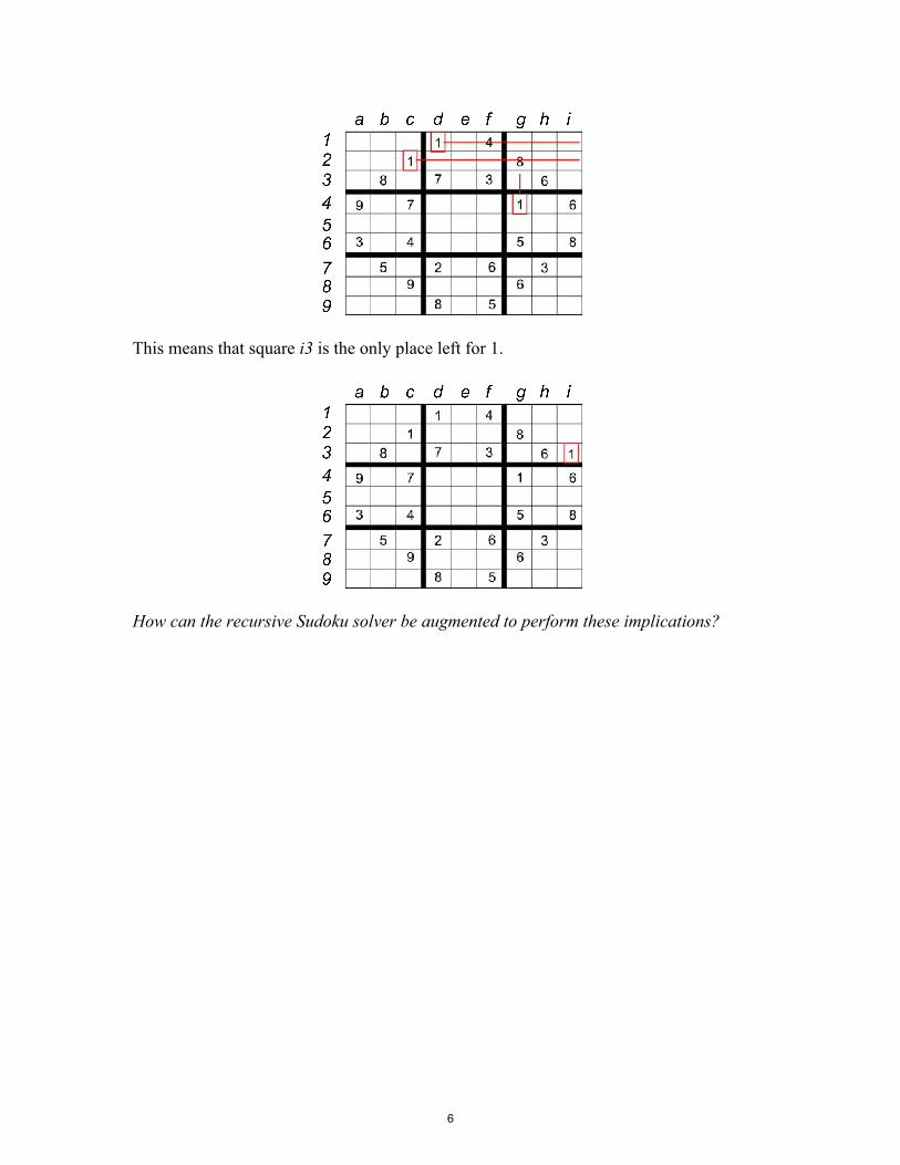
This means that square i3 is the only place left for 1.

How can the recursive Sudoku solver be augmented to perform these implications?

6

Implications During Recursive Search We will show how to augment our solver to perform this implication and see how much more efficient the solver becomes. We can do this by measuring the number of backtracks with and without implications. Implications more quickly determine whether a particular assignment of values to empty squares is correct or not. There are several changes that need to be made to the solver in order to correctly implement this optimization. To be clear, this optimization is thought of as an implication because the current state of the grid implies a position for the 1 in the example above. There can be one or more implications that can be made once a particular grid location is assigned a value. The recursive search code in the optimized solver needs to be slightly different.  1.   backtracks  =  0      2.   def  solveSudokuOpt(grid,  i  =  0,  j  =  0):    3.          global  backtracks        4.          i,  j  =  findNextCellToFill(grid)    5.          if  i  ==  -­‐1:    6.                  return  True    7.          for  e  in  range(1,  10):    8.                  if  isValid(grid,  i,  j,  e):    9.                          impl  =  makeImplications(grid,  i,  j,  e)10.                          if  solveSudoku(grid,  i,  j):  11.                                  return  True  12.                          backtracks  +=  1  13.                          undoImplications(grid,  impl)  14.          return  False  

 

The only changes are on Lines 9 and 13. On Line 9, not only are we filling in the grid[i][j] entry with e but we are also making implications and filling in other grid locations. All of these have to be “remembered” in the implication list impl. On Line 13, we have to undo all of the changes made to the grid because the grid[i][j]  =  e guess was incorrect. Storing the assignment and implications performed so we can roll them all back if the assignment does not work is important for correctness – else we might not explore the entire search space and therefore not find a solution. To understand this, look at the figure below.

7

Think of A, B and C above as being grid locations and assume that we only have two numbers 1 and 2 that are possible entries. (We have a simplified situation for illustration purposes.) Suppose we assign A = 1, B = 1, and then C = 2 is implied. After exploring the A = 1, B = 1 branch fully, we backtrack to A = 1, B = 2. Here, we need to explore C = 1 and C = 2 as in the picture to the left, not just C = 2 as shown on the picture to the right. What might happen is that C is still set to 2 in the B = 2 branch and we, in effect, only explore the B = 2, C = 2 branch. So we need to roll back all the implications associated with an assignment. The procedure undoImplications is short and is shown below. 1.   def  undoImplications(grid,  impl):  2.          for  i  in  range(len(impl)):  3.                  grid[impl[i][0]][impl[i][1]]  =  0   impl is a list of 3-tuples, where each 3-tuple is of the form (i,  j,  e) meaning that grid[i][j]  =  e. In undoImplications we don’t care about the third item e since we want to empty out the entry. makeImplications is more involved since it performs significant analysis. The pseudocode for makeImplications is below. The line numbers are for the Python code that is shown after the pseudocode. For each sector (sub-grid): Find missing elements in the sector (Lines 8-12) Attach set of missing elements to each empty square in sector (Lines 13-16) For each empty square S in sector: (Lines 17-18) Subtract all elements on S’s row from missing elements set (Lines 19-22) Subtract all elements on S’s column from missing elements set (Lines 23-26) If missing elements set is a single value then: (Line 27) Missing square value can be implied to be that value (Lines 28-31)

8

 1.   sectors  =  [[0,  3,  0,  3],  [3,  6,  0,  3],  [6,  9,  0,  3],                                    [0,  3,  3,  6],  [3,  6,  3,  6],  [6,  9,  3,  6],                                    [0,  3,  6,  9],  [3,  6,  6,  9],  [6,  9,  6,  9]]      2.   def  makeImplications(grid,  i,  j,  e):    3.          global  sectors    4.          grid[i][j]  =  e    5.          impl  =  [(i,  j,  e)    6.          for  k  in  range(len(sectors)):    7.                  sectinfo  =  []    8.                  vset  =  {1,  2,  3,  4,  5,  6,  7,  8,  9}    9.                  for  x  in  range(sectors[k][0],  sectors[k][1]):  10.                          for  y  in  range(sectors[k][2],  sectors[k][3]):  11.                                  if  grid[x][y]  !=  0:  12.                                          vset.remove(grid[x][y])  13.                  for  x  in  range(sectors[k][0],  sectors[k][1]):  14.                          for  y  in  range(sectors[k][2],  sectors[k][3]):  15.                                  if  grid[x][y]  ==  0:  16.                                          sectinfo.append([x,  y,  vset.copy()])              17.                  for  m  in  range(len(sectinfo)):  18.                          sin  =  sectinfo[m]                          19.                          rowv  =  set()  20.                          for  y  in  range(9):  21.                                  rowv.add(grid[sin[0]][y])  22.                          left  =  sin[2].difference(rowv)                      23.                          colv  =  set()  24.                          for  x  in  range(9):  25.                                  colv.add(grid[x][sin[1]])  26.                          left  =  left.difference(colv)                                                    27.                          if  len(left)  ==  1:  28.                                  val  =  left.pop()  29.                                  if  isValid(grid,  sin[0],  sin[1],  val):  30.                                          grid[sin[0]][sin[1]]  =  val  31.                                          impl.append((sin[0],  sin[1],  val))                      32.          return  impl  

       

Line 1 declares variables that give the grid indices of each of the 9 sectors. For example, the middle sector 4 varies from 3 to 5 inclusive in the x and y coordinates. This is helpful in ranging over the grid but staying within a sector. This code uses the set data structure in Python. An empty set is declared using set() as opposed to an empty list which is declared as []. A set cannot have repeated elements. Note that even if we included a number, say 1, twice in the declaration of a set, it would only be included once in the set. V  =  {1,  1,  2} is the same as V  =  {1,  2}. Line 8 declares a set vset that contains numbers 1 through 9. In Lines 9-12, we go through the elements in the sector and remove these elements from vset using the remove function. We wish to append this missing element set to each empty square and hence we create a list sectinfo of 3-tuples. Each 3-tuple has the x, y coordinates of the

9

empty square in the sector, and a copy of the set of missing elements in the sector. We need to make copies of sets because these copies will diverge in their membership later in the algorithm. For each empty square in the sector, we look at the corresponding 3-tuple in sectinfo (Line 18). The elements that are in the corresponding row are removed from the missing element set given by sin[2], the third element of the 3-tuple by using the set difference function (Line 22). Similarly, for the column associated with the empty square. The remaining elements are stored in the set left. If the set left has cardinality 1 (Line 27), we may have an implication. Why are we not guaranteed an implication? The way we have written the code, we compute the missing elements for each sector, and try to find implications for each empty square in the sector. The very first implication will hold, but once we make one particular implication, the sector changes as does the missing elements set. So further implications computed using stale missing elements information may not be valid. This is why we check if the implication violates the rules of Sudoku on Line 29 prior to including it in the implication list impl. This optimization shrinks the number of backtracks down from 579 to 10 for the puzzle input and from 6,363 to 33 for puzzle inp2. Of course, from a standpoint of computer time usage, both versions run in fractions of a second! This is one of the reasons why we included the functionality of counting backtracks in the code so you could see that the optimizations do help reduce the guessing required.

Difficulty of Sudoku Puzzles A Finnish mathematician Arto Inkala claimed in 2006 claimed he had created the world’s hardest Sudoku puzzle and followed it up in 2010 with a claim of an even harder puzzle. The first puzzle takes the unoptimized solver 335,578 backtracks and the second 9949 backtracks! The solver finds solutions in a matter of seconds. To be fair, Inkala was predicting human difficulty. Here’s Inkala’s 2010 puzzle below.

10

Peter Norvig has written Sudoku solvers that use constraint programming techniques significantly more sophisticated than the simple implications we have presented here. As a result the amount of backtracking required even for difficult puzzles is quite small. We suggest you find Sudoku puzzles with different levels of difficulty, from easy to very hard and explore how the number of backtracks required in the basic solver and the optimized solver change as the level of difficulty increases. You might be surprised by what you find!

Exercises Exercise 1: We’ll improve our optimized (classic) Sudoku solver in this exercise. Each time we discover an implication, the grid changes, and we may find other implications. In fact, this is the way humans solve Sudoku puzzles. Our optimized solver goes through all the sectors trying to find implications, and then stops. If we find an implication in one “pass” through the grid sectors, we could try repeating the entire process (Lines 6-31) until we can’t find implications, i.e., can’t add to our data structure impl. Code this improved Sudoku solver. What you have to do is enclose the process in a while loop and exit when there are no changes. Be careful with indentation and properly initializing variables! You should get Backtracks = 2 in your improved solver for Sudoku puzzle inp2, down from 33. Puzzle Exercise 2: Modify the basic Sudoku solver to work with Diagonal Sudoku, where there is an additional constraint that all the numbers 1 through 9 must appear on the both diagonals. Below is a Diagonal Sudoku puzzle:

And here is its solution:

11

Puzzle Exercise 3: Modify the basic Sudoku solver to work with Even Sudoku, which is similar to classic Sudoku, except that particular squares have to have even numbers. An example is given below.

Tbe grayed out blank squares have to contain even numbers; the other squares can contain either odd or even numbers. To represent the puzzle using a 2-dimensional list, we will use 0’s as before to indicate blank squares without additional constraints, and -2’s to indicate that the square is blank and has to contain an even number. Therefore, the input list for the above puzzle is:

even  =  [[8,  4,  0,  0,  5,  0,-­‐2,  0,  0],                  [3,  0,  0,  6,  0,  8,  0,  4,  0],                  [0,  0,-­‐2,  4,  0,  9,  0,  0,-­‐2],                  [0,  2,  3,  0,-­‐2,  0,  9,  8,  0],                  [1,  0,  0,-­‐2,  0,-­‐2,  0,  0,  4],                  [0,  9,  8,  0,-­‐2,  0,  1,  6,  0],                  [-­‐2,0,  0,  5,  0,  3,-­‐2,  0,  0],                  [0,  3,  0,  1,  0,  6,  0,  0,  7],                  [0,  0,-­‐2,  0,  2,  0,  0,  1,  3]]  

The solution to the above puzzle is:

12

 

13

MIT OpenCourseWarehttps://ocw.mit.edu

6.S095 Programming for the PuzzledJanuary IAP 2018

For information about citing these materials or our Terms of Use, visit: https://ocw.mit.edu/terms.