Program Static Analysis - Virginia...

4/19/16

1

Program Static Analysis

Overview

•  Program static analysis •  Abstract interpretation •  Data flow analysis – Intra-procedural – Inter-procedural

2

4/19/16

2

What is static analysis?

•  The analysis to understand computer software without executing programs – Simple coding style •  Empty statement, EqualsHashcode

– Complex property of the program •  the program’s implementation matches its

specification – “Given program P and specification S, does P

satisfy S ?” •  Can be conducted on source code or

object code 3

Has anyone done static analysis?

•  Code review •  …

4

4/19/16

3

Why static analysis?

•  Program comprehension – Is this value a constant?

•  Bug finding – Is a file closed on every path after all its

access? •  Program optimization – Constant propagation

5

An Informal Introduction to Abstract Interpretation

Patrick Cousot[2] Modified by Na Meng

4/19/16

4

Semantics & Safety

•  The concrete semantics of a program formalizes (is a mathematical model of) the set of all its possible executions in all possible execution environments

•  Safety: No possible execution in any possible execution environment can reach an erroneous state

7

Undecidability

•  The concrete semantics of a program is undecidable – Given an arbitrary program, can you prove

that it halts or not on any possible input? – Turing proved no algorithm can exist that

always correctly decides whether, for a given arbitrary program and its input, the program halts when run with that input

8

4/19/16

5

Abstract Semantics

•  A sound approximation (superset) of the concrete semantics

•  It covers all possible concrete cases •  If the abstract semantics is proved to be

safe, then so is the concrete semantics •  Abstract interpretation – abstract semantics + proof of safe

properties

9

Why is Testing/Debugging insufficient?

•  Only consider a subset of the possible executions

•  No correctness proof •  No guarantee of full coverage of

concrete semantics

10

4/19/16

6

Static Analysis Techniques

•  Model checking •  Theorem proving •  Data flow analysis

11

Model Checking

•  The abstract semantics is modeled as a finite state machine of the program execution

•  The model can be manually defined or automatically computed

•  Each state is enumerated exhaustively to automatically check whether this model meets a given specification

12

4/19/16

7

13

import java.util.Random; public class Rand {

public static void main (String[] args) { Random random = new Random(42);// (1) int a = random.nextInt(2); // (2) System.out.println("a=" + a);

... ... int b = random.nextInt(3); // (3) System.out.println(" b=" + b); int c = a/(b+a - 2); // (4) System.out.println(" c=" + c); }

}

An Example [3]

Is there any Divide-by-Zero

error?

Model Checking

14

start a=0 a=1

5 6 7 8

c=0 c=0/0 c=-1 c=1/0 c=1

①  Random random = new Random() ②  int a = random.nextInt(2)

③  int b = random.nextInt(3)

④  int c = a/(b+a-2)

1 2 b=0

b=1 b=2 b=0

b=1 b=2

4 3

9 10 11 12 13

What if there is any loop?

4/19/16

8

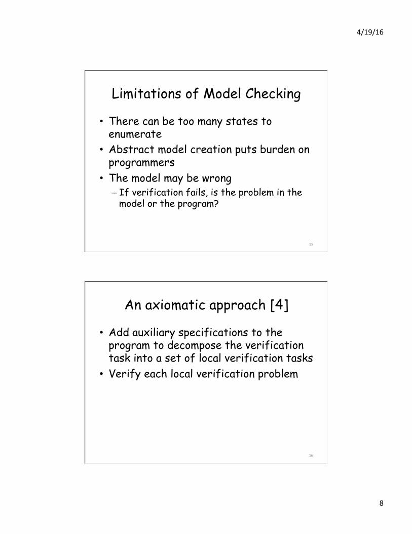
Limitations of Model Checking

•  There can be too many states to enumerate

•  Abstract model creation puts burden on programmers

•  The model may be wrong – If verification fails, is the problem in the

model or the program?

15

An axiomatic approach [4]

•  Add auxiliary specifications to the program to decompose the verification task into a set of local verification tasks

•  Verify each local verification problem

16

4/19/16

9

Limitations

•  Auxiliary spec is burden on programmers •  Auxiliary spec might be incorrect •  If verification fails, is the problem with

the auxiliary specification or the program?

17

Theorem Proving

18

Meets spec/Found Bug

Theorem in a logic

Program

Specification

Semantics

VC generation

Validity

Provability (theorem proving)

•  Soundness – If the theorem is valid then the program

meets specification – If the theorem is provable then it is valid

4/19/16

10

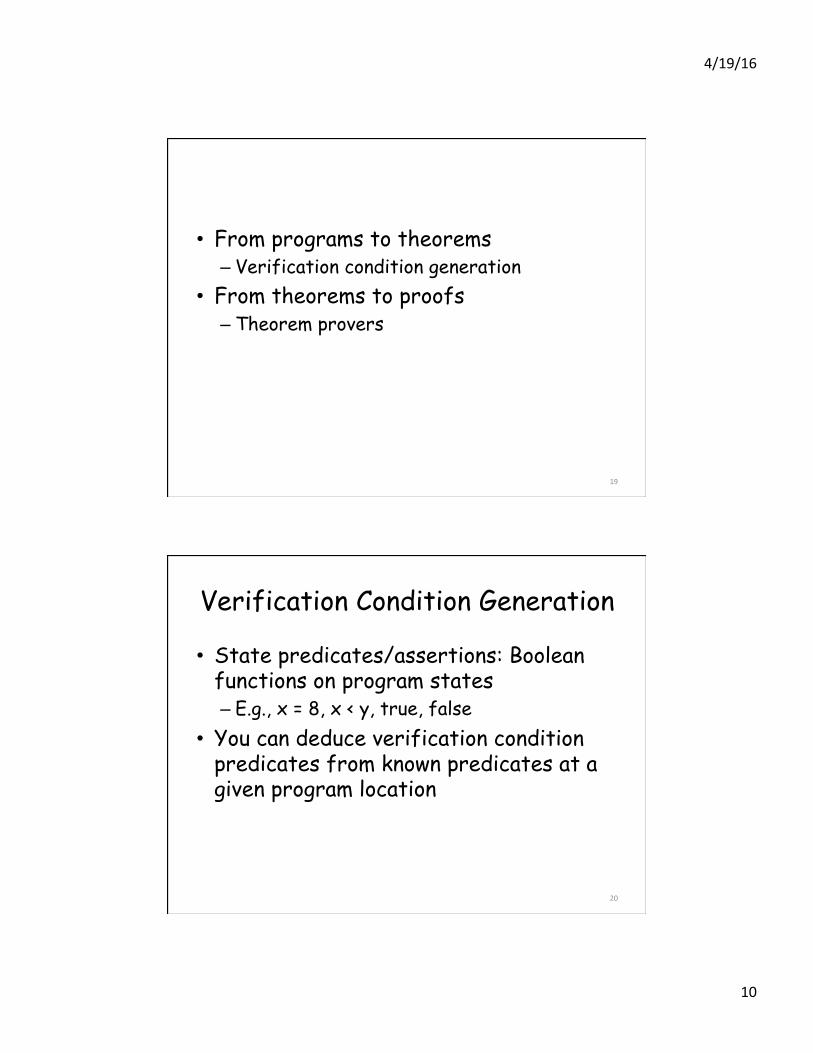
•  From programs to theorems – Verification condition generation

•  From theorems to proofs – Theorem provers

19

Verification Condition Generation

•  State predicates/assertions: Boolean functions on program states – E.g., x = 8, x < y, true, false

•  You can deduce verification condition predicates from known predicates at a given program location

20

4/19/16

11

Hoare Triples [6]

•  For any predicates P and Q and program S,

says that if S is started in a state satisfying P, then it terminates in Q – E.g., {true} x := 12 {x = 12}, {x < 40} x := x+1 {x ≤

40}

21

postcondi5on

precondi5on

{P} S {Q}

Precise Triples

•  If {P} S {Q ∧ R} holds, then do {P} S {Q} and {P} S {R} hold?

•  Strongest postcondition – The most precise postcondition (Q ∧ R),

which implies any postcondition satisfied by the final state of any execution x of S

– E.g., {true} x := 12 {x = 12} vs. {true} x:=12 {x > 0}, which postcondition is stronger?

22

4/19/16

12

Precise Triples

•  If {P} S {R} or {Q} S {R} hold, then does {P ∨ Q} S {R} hold?

•  Weakest preconditions – The most general precondition {P ∨ Q}, is the

“weakest” precondition on the initial state ensuring that execution of S terminates in a final state satisfying R.

– E.g., {x=13} x = x+3 {x >13} vs. {x>10} x = x+3 {x >13}, which precondition is weaker?

23

Example: Does the program satisfy the specification?

•  Specification requires true (precondition) ensures c = a ∨ b (postcondition)

•  Program

24

bool or(bool a, bool b) { if (a) c := true; else c := b; return c }

4/19/16

13

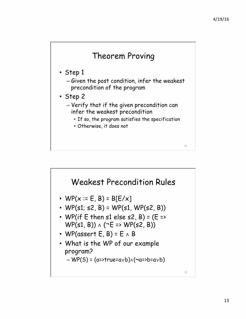
Theorem Proving

•  Step 1 – Given the post condition, infer the weakest

precondition of the program •  Step 2 – Verify that if the given precondition can

infer the weakest precondition •  If so, the program satisfies the specification •  Otherwise, it does not

25

Weakest Precondition Rules

26

•  WP(x := E, B) = B[E/x] •  WP(s1; s2, B) = WP(s1, WP(s2, B)) •  WP(if E then s1 else s2, B) = (E =>

WP(s1, B)) ∧ ( E => WP(s2, B)) •  WP(assert E, B) = E ∧ B •  What is the WP of our example

program? – WP(S) = (a=>true=a∨b)∧( a=>b=a∨b)

¬

¬

4/19/16

14

•  Conjecture to be proved: – true=> (a=>true=a∨b)∧( a=>b=a∨b)

27

Data Flow Analysis [5]

Peter Lee Modified by Na Meng

4/19/16

15

Data Flow Analysis

•  A technique to gather information about the possible set of values calculated at various points in a computer program

29

How to do data flow analysis?

•  Set up data-flow equations for each node of the control flow graph

•  Solve the equation set iteratively, until

reaching a fixpoint: all in-states do not change

30

outb = trans(inb )inb = joinp∈predb (outp )

for i ← 1 to N initialize node i while (sets are still changing) for i ← 1 to N recompute sets at node i

4/19/16

16

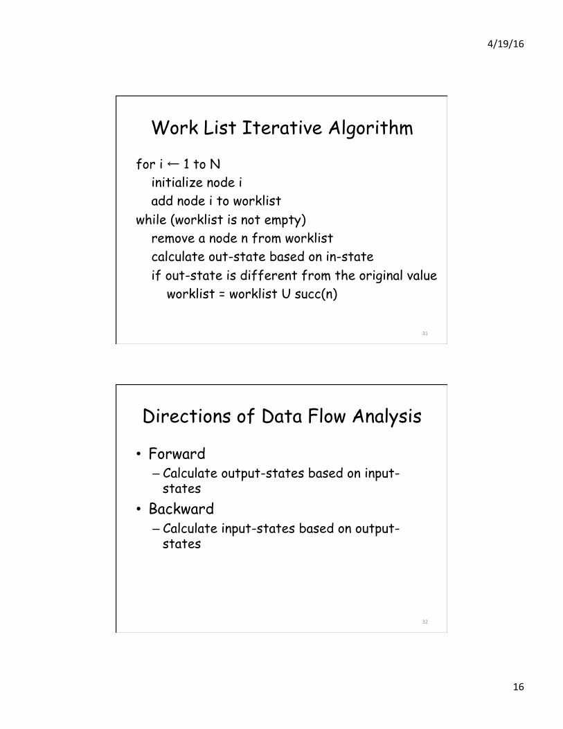
Work List Iterative Algorithm

for i ← 1 to N initialize node i add node i to worklist while (worklist is not empty) remove a node n from worklist calculate out-state based on in-state if out-state is different from the original value worklist = worklist U succ(n)

31

Directions of Data Flow Analysis

•  Forward – Calculate output-states based on input-

states •  Backward – Calculate input-states based on output-

states

32

4/19/16

17

An Example [7]

1: int N = input() 2: initialize array A[N + 1] 3: call check(N) 4: int I = 1 5: while (I < N) { 6: A(I) = A(I) + I 7: I = I + 1 } 8: print A(N) 33

1

2

4

5

6

7

8

entry

exit

•  What variable definitions reach the current program point?

3

Reaching Definition

•  A definition at program point d reaches program point u if there is a control-flow path from d to u that does not contain a definition of the same variable as d

34

4/19/16

18

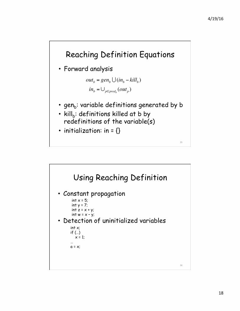
Reaching Definition Equations •  Forward analysis

•  genb: variable definitions generated by b •  killb: definitions killed at b by

redefinitions of the variable(s) •  initialization: in = {}

35

inb =∪p∈predb(outp )

outb = genb ∪ (inb − killb )

Using Reaching Definition

•  Constant propagation

•  Detection of uninitialized variables

36

int x = 5; int y = 7; int z = x + y; int w = x – y;

int x; if (…) x = 1; … a = x;

4/19/16

19

Using Reaching Definition

•  Loop-invariant Code Motion – Consider an expression inside a loop. If all

reaching definitions are outside of the loop, then move the expression out of the loop

37

Revisit the Example[7]

1: int N = input() 2: initialize array A[N + 1] 3: call check(N) 4: int I = 1 5: while (I < N) { 6: A(I) = A(I) + I 7: I = I + 1 } 8: print A(N) 38

1

2

4

5

6

7

8

entry

exit

•  What variable definitions are or will be actually used?

3

4/19/16

20

Live-out Variables

•  A variable v is live-out of statement n if v is used along some control path starting at n. Otherwise, we say that v is dead – “What variables definitions are actually

used?”

39

Liveness Analysis Equations

•  Backward analysis

•  genb: variables used by b •  killb: if v is defined without using v, all

its prior definitions are killed •  initialization: out = {}

40

outb =∪p∈succb(inp )

inb = outb − killb∪genb

4/19/16

21

Using Liveness Analysis

•  Dead code elimination – Suppose we have a statement defining a

variable, whose value is not used, then the definition can be removed without any side effect

41

Available Expression

•  An expression e is available at statement n if –  it is computed along every path from entry

node to n, and – no variable used in e gets redefined

between e’s computation and n

42

4/19/16

22

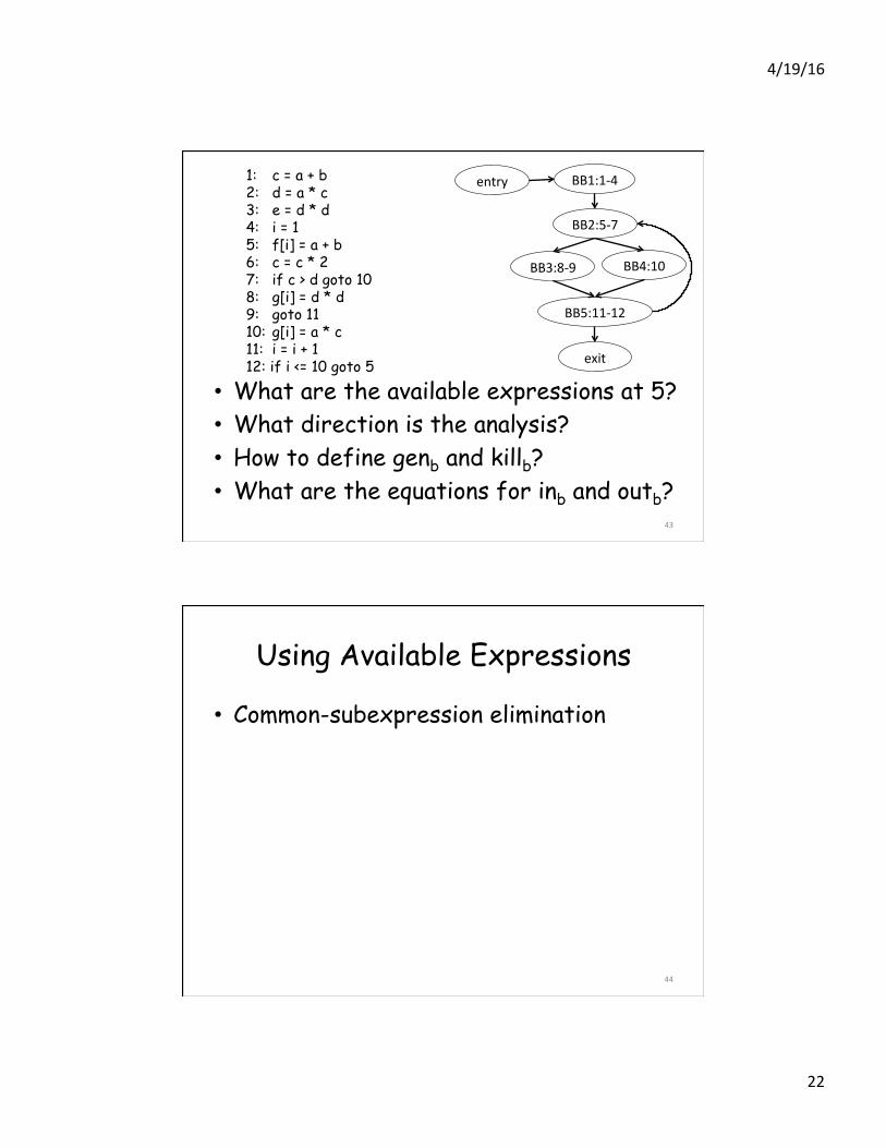
•  What are the available expressions at 5? •  What direction is the analysis? •  How to define genb and killb? •  What are the equations for inb and outb?

43

1: c = a + b 2: d = a * c 3: e = d * d 4: i = 1 5: f[i] = a + b 6: c = c * 2 7: if c > d goto 10 8: g[i] = d * d 9: goto 11 10: g[i] = a * c 11: i = i + 1 12: if i <= 10 goto 5

BB1:1-‐4

BB2:5-‐7

BB3:8-‐9 BB4:10

BB5:11-‐12

entry

exit

Using Available Expressions

•  Common-subexpression elimination

44

4/19/16

23

Our analyses so far

45

Reaching definitions

Available expressions

Live variables

back

ward

for

ward

union intersection

Questions

•  Does work list iterative algorithm always terminate?

46

4/19/16

24

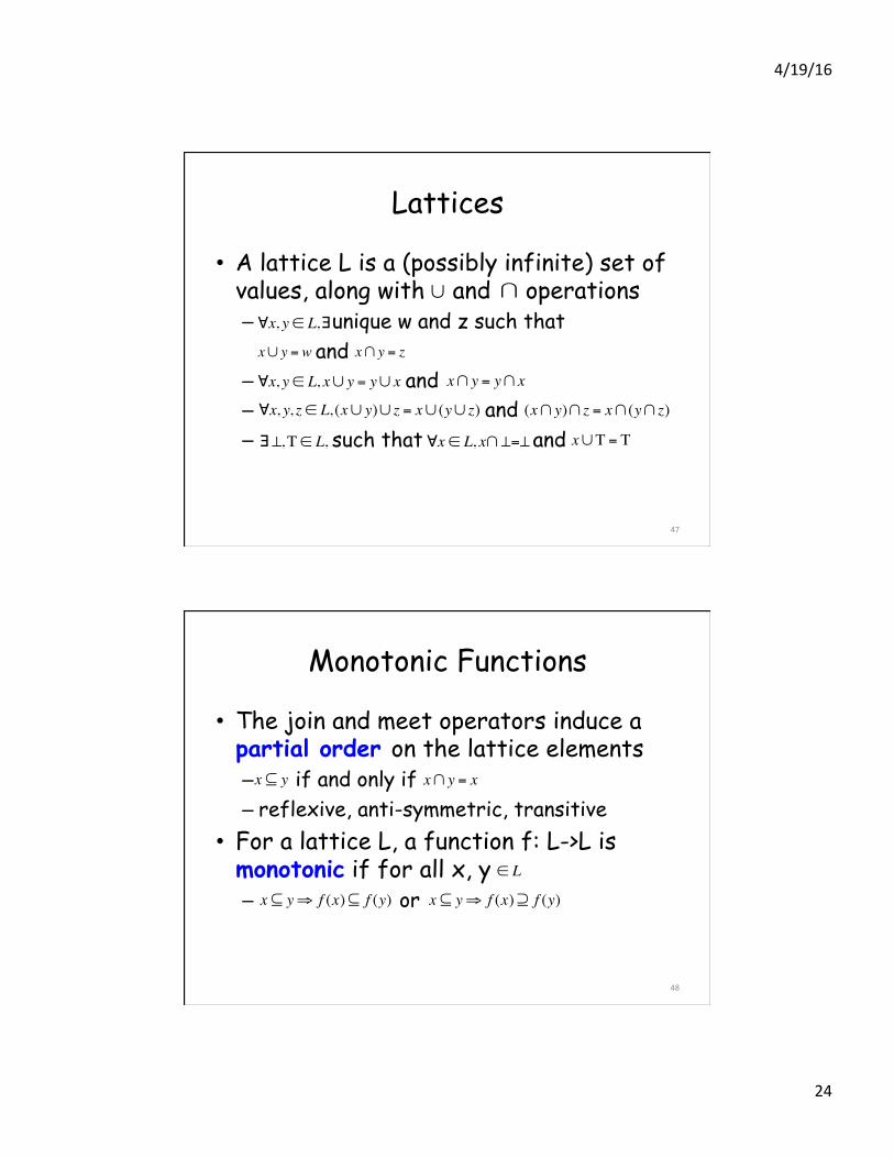
Lattices

•  A lattice L is a (possibly infinite) set of values, along with and operations –  unique w and z such that and –  and –  and –  such that and

47

∪ ∩

∀x, y ∈ L,∃

x∪ y = w x∩ y = z

∀x, y ∈ L, x∪ y = y∪ x x∩ y = y∩ x

∀x, y, z ∈ L, (x∪ y)∪ z = x∪ (y∪ z) (x∩ y)∩ z = x∩ (y∩ z)

∃⊥,Τ ∈ L, ∀x ∈ L, x∩⊥=⊥ x∪Τ = Τ

Monotonic Functions

•  The join and meet operators induce a partial order on the lattice elements –  if and only if – reflexive, anti-symmetric, transitive

•  For a lattice L, a function f: L->L is monotonic if for all x, y –  or

48

x ⊆ y x∩ y = x

∈ L

x ⊆ y⇒ f (x)⊆ f (y) x ⊆ y⇒ f (x)⊇ f (y)

4/19/16

25

Reaching definition is monotonic

•  Proof (for single-variable single-block programs) by contradiction: – Suppose , where 1 means

there is a variable definition, 0 means no definition, then .

– However, only if the block b has a redefinition of the variable, which means

49


inb = {1},outb = {0}

genb = {0},killb = {1}killb = {1}

genb = {1}

•  Therefore, after limited number of iterations (N* (E+1) at worst case), every definition is propagated to every node

•  Therefore, we can find a fixpoint p, such that f(p) = p

50

4/19/16

26

In dataflow analysis, we require that all flow functions be monotone

and have only finite-length effective chains

Ingredients of a Dataflow Analysis

•  Flow direction •  Transfer function •  Meet operator (Join function) •  Dataflow information – Set of definitions, variables, and

expressions –  initialization – How about concrete data values?

52

4/19/16

27

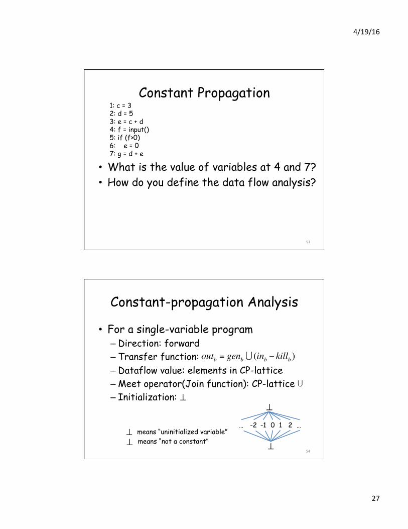
Constant Propagation

53

1: c = 3 2: d = 5 3: e = c + d 4: f = input() 5: if (f>0) 6: e = 0 7: g = d + e

•  What is the value of variables at 4 and 7? •  How do you define the data flow analysis?

Constant-propagation Analysis

•  For a single-variable program – Direction: forward – Transfer function: – Dataflow value: elements in CP-lattice – Meet operator(Join function): CP-lattice – Initialization:

54

⊥


∪

⊥

⊥

-2 -1 0 1 2 … … ⊥ means “uninitialized variable”

means “not a constant” ⊥

4/19/16

28

Inter-procedural Analysis [8]

Stephen Chong Imported by Na Meng

Procedures

•  So far we have looked at intra-procedural analysis: analyzing a single procedure

•  Inter-procedural analysis uses calling relationships among procedures – Connect intra-procedural analysis results

via call edges – Enable more precise analysis information

56

4/19/16

29

Inter-procedural CFG void main() { x = 7; r = p(x); x = r; z = p(x+10); } int p(int a) { int y; if (a < 9) y = 0; else y = 1; return y; } 57

Entry main

x = 7

call p(x)

r = return p(x)

x = r

call p(x+10)

z = return p(x+10)

Exit main

Entry p

a < 9

y = 0 y = 1

return y;

Exit p

Imprecision

•  Dataflow facts from one call site can “taint” results at other call sites – Is z a constant?

58

4/19/16

30

Inlining •  Make a copy of the callee’s CFG at each

call site

59

Entry main

x := 7

Call p(x)

r := Return p(x)

x := r

Call p(x+10)

z := return p(x+10)

Exit main

Entry p

a < 9

y := 0 y := 1

return y;

Exit p

Entry p

a < 9

y := 0 y := 1

return y;

Exit p

Exponential Size Increase

•  How about recursive function calls? – p(int n) {… p(n - 1);…}

•  The exponential increase makes analysis infeasible

60

4/19/16

31

Context Sensitivity

•  Make a finite number of copies •  Use context information to determine

when to share a copy – Different decisions achieve different

tradeoffs between precision and scalability •  Common choice: approximation call stack

61

An Example

62

Context insensitivity

main

b() e()

c() f()

d() g()

Context sensitive, 1-stack depth

main

b() e()

c() f()

d() g()

c()

d()

f()

g()

Context sensitive, 2-stack depth

main

b() e()

c() f()

d g

c()

d

f()

g d g d g

4/19/16

32

Procedure Summaries

•  In practice, people don’t construct a single global CFG and then perform dataflow

•  Instead, construct and use procedure summaries

•  Summarize effect of callees on callers – E.g., is there any side effect on callers?

•  Summarize effect of callers on callees – E.g., is any parameter constant?

63

Other Contexts

•  Object/pointer sensitivity – What is the type of a given object and

what are the corresponding possible method targets?

– What is the value of a given object’s field?

64

4/19/16

33

Pointer Analysis

65

•  What is the points-to set of p? int x = 3; int y = 0; int* p = unknown() ? &x : & y;

•  Alias analysis – Decide whether separate memory

references point to the same area of memory

– Can be used interchangeably with pointer analysis (points-to analysis)

Flow Sensitivity

•  Flow insensitive analysis – Perform analysis without caring about the

statement execution order •  E.g., analysis of c1;c2 will be the same as c2;c1 •  Address-taken, Steensgaard, Anderson

•  Flow sensitive analysis – Observes the statement execution order

66

4/19/16

34

An Example

1: a = &b 2: b = &c 3: f = &d 4: d = &e 5: a = f

67

a -> b -> c f -> d -> e

1 2

3 4

•  After 5, both *a and *f point to d

Address Taken

•  Assume that variables whose addresses are taken may be referenced by all pointers – Address-taken variables: b, c, d, e – A single alias pointer set: {a, b, f, d}

68

1: a = &b 2: b = &c 3: f = &d 4: d = &e 5: a = f

a -> b -> c f -> d -> e

1 2

3 4

4/19/16

35

Steensgaard

•  Constraints – p = &x: x pts-to(p) – p = q: pts-to(p) = pts-to(q) – p = *q pts-to(q), pts-to(p)=pts-to(a) – *p = q pts-to(p), pts-to(b)=pts-to(q)

69

∈

∀a ∈

∀b∈

1: a = &b 2: b = &c 3: f = &d 4: d = &e 5: a = f

a -> b -> c f -> d -> e

1 2

3 4 -> ->

– Points-to set: pts(a) = pts(f) ={b, d}

Andersen

•  Subset Constraints – p = &x: x pts-to(p) – p = q: pts-to(q) pts-to(p) – p = *q pts-to(q), pts-to(a) pts-to(a) – *p = q pts-to(p), pts-to(q) pts-to(b)

70

∈

∀a ∈

∀b∈

⊆

⊆

⊆

1: a = &b 2: b = &c 3: f = &d 4: d = &e 5: a = f

a -> b -> c f -> d -> e

1 2

3 4

– Points-to set: pts(a)={b, d}, pts(f)={d}

->

4/19/16

36

Flow-sensitive Pointer Analysis

•  x = y: strong update – kill—clear pts(x) – gen—add pts(y) to pts(x)

•  *x = y: – If x definitely points to a single concrete

memory location z, pts(z) = y (strong update) – If x may point to multiple locations, then week update by adding y to pts of all locations 71

inb =∪p∈predb(outp )


Reference [1] Static program analysis, https://en.wikipedia.org/wiki/Static_program_analysis [2] Patrick Cousot, A Tutorial on Abstract Interpretation, http://homepage.cs.uiowa.edu/~tinelli/classes/seminar/Cousot--A%20Tutorial%20on%20AI.pdf [3] Software Model Checking Example, http://javapathfinder.sourceforge.net/sw_model_checking.html [4] Automated Theorem Proving, https://courses.cs.washington.edu/courses/cse599f/06sp/lectures/atp1.ppt [5] Peter Lee, Classical Dataflow Optimizations, http://www.cs.cmu.edu/afs/cs/academic/class/15745-s06/web/handouts/04.pdf [6] K. Rustan M. Leino, Hoare-style program verification, http://research.microsoft.com/en-us/um/people/leino/papers/cse503-Leino-Lecture0.ppt.

72

4/19/16

37

Reference

[7] Kathryn S. McKinley, Data Flow Analysis and Optimizations, http://www.cs.utexas.edu/users/mckinley/380C/lecs/03.pdf [8] Stephen Chong, Interprocedural Analysis, http://www.seas.harvard.edu/courses/cs252/2011sp/slides/Lec05-Interprocedural.pdf 73

Program Static Analysis - Virginia...

Documents

Transcript of Program Static Analysis - Virginia...