Program Optimization - TUM

Program Optimization

Peter Lammich

WS 2016/17

1 / 471

Overview by Lecture• Oct 20: Slide 3• Oct 26: Slide 36• Oct 27: Slide 65• Nov 3: Slide 95• Nov 9: Slide 116• Nov 10: Slide 128• Nov 16: Slide 140• Nov 17: Slide 157• Nov 23: Slide 178• Nov 24: Slide 202• Nov 30: Slide 211• Dec 1: Slide 224• Dec 8: Slide 243• Dec 14: Slide 259• Dec 15: Slide 273• Dec 21: Slide 287• Dec 22: Slide 301• Jan 11,12: Slide 320• Jan 18,19: Slide 348• Jan 25,26: Slide 377• Feb 1,2: Slide 408• Feb 8,9: Slide 435

2 / 471

Organizational Issues

Lectures Wed 10:15-11:45 and Thu 10:15-11:45 in MI 00.13.009ATutorial Fri 8:30-10:00 (Ralf Vogler <[email protected]>)

• Homework will be correctedExam Written (or Oral), Bonus for Homework!

• ≥ 50% of homework =⇒ 0.3/0.4 better gradeOn first exam attempt. Only if passed w/o bonus!

Material Seidl, Wilhelm, Hack: Compiler Design: Analysis andTransformation, Springer 2012

How many of you are attending “Semantics” lecture?

3 / 471

Info-2 Tutors

We need tutors for Info II lecture. Ifyou are interested, please contact

Julian [email protected].

4 / 471

[email protected]

Proposed Content

• Avoiding redundant computations• E.g. Available expressions, constant propagation, code motion

• Replacing expensive with cheaper computations• E.g. peep hole optimization, inlining, strength reduction

• Exploiting Hardware• E.g. instruction selection, register allocation, scheduling

• Analysis of parallel programs• E.g. threads, locks, data-races

5 / 471

Table of Contents

1 Introduction

2 Removing Superfluous Computations

3 Abstract Interpretation

4 Alias Analysis

5 Avoiding Redundancy (Part II)

6 Interprocedural Analysis

7 Analysis of Parallel Programs

8 Replacing Expensive by Cheaper Operations

9 Exploiting Hardware Features

10 Optimization of Functional Programs

6 / 471

Observation 1

Intuitive programs are often inefficient

void swap (int i, int j) {int t;if (a[i] > a[j]) {t = a[j];a[j] = a[i];a[i] = t;

}}

• Inefficiencies• Addresses computed 3 times• Values loaded 2 times

• Improvements• Use pointers for array indexing• Store the values of a[i], a[j]

7 / 471

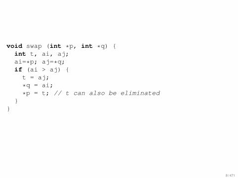
void swap (int *p, int *q) {int t, ai, aj;ai=*p; aj=*q;if (ai > aj) {t = aj;

*q = ai;

*p = t; // t can also be eliminated}

}

8 / 471

void swap (int *p, int *q) {int ai, aj;ai=*p; aj=*q;if (ai > aj) {

*q = ai;

*p = aj;}

}

Caveat: Program less intuitive

9 / 471

Observation 2

High-level languages (even C) abstract from hardware (and efficiency)Compiler needs to transform intuitively written programs to hardware.Examples• Filling of delay slots• Utilization of special instructions• Re-organization of memory accesses for better cache behavior• Removal of (useless) overflow/range checks

10 / 471

Observation 3

Program improvements need not always be correct• E.g. transform f() + f() to 2*f()• Idea: Save second evaluation of f• But what if f has side-effects or reads input?

11 / 471

Insight

• Program optimizations have preconditions• These must be

• Formalized• Checked

• It must be proved that optimization is correct• I.e., preserves semantics

12 / 471

Observation 4

Optimizations techniques depend on programming language• What inefficiencies occur• How analyzable is the language• How difficult it is to prove correctness

13 / 471

Example: Java

• (Unavoidable) inefficiencies• Array bound checks• Dynamic method invocation• Bombastic object organization

• Analyzability+ No pointer arithmetic, no pointers into stack- Dynamic class loading- Reflection, exceptions, threads

• Correctness proof+ Well-defined semantics (more or less)- Features, features, features- Libraries with changing behavior

14 / 471

In this course

• Simple imperative programming languageR = e AssignmentR = M[e] LoadM[e1] = e2 Storeif (e) ... else ... Conditional branchinggoto label Unconditional branching

R Registers, assuming infinite supplye Integer-valued expressions over constants, registers, operatorsM Memory, addressed by integer ≥ 0, assuming infinite memory

15 / 471

Note

• For the beginning, we omit procedures• Focus on intra-procedural optimizations• External procedures taken into account via statement f()

• unknown procedure• may arbitrarily mess around with memory and registers

• Intermediate Language, in which (almost) everything can be translated

16 / 471

Example: Swap

void swap (int i, int j) {int t;if (a[i] > a[j]) {t = a[j];a[j] = a[i];a[i] = t;

}}

Assume A0 contains address of array a

1: A1 = A0 + 1*i //R1 = a[i]

2: R1 = M[A1]3: A2 = A0 + 1*j //R2 = a[j]

4: R2 = M[A2]5: if (R1 > R2) {

6: A3 = A0 + 1*j //t=a[j]

7: t = M[A3]8: A4 = A0 + 1*j //a[j] = a[i]

9: A5 = A0 + 1*i

0: R3 = M[A5]1: M[A4] = R32: A6 = A0 + 1*i //a[i]=t

3: M[A6] = t

}

17 / 471

Optimizations

1 1 * R 7→ R

2 Re-use of sub-expressionsA1 == A5== A6, A2 == A3== A4

M[A1] == M[A5], M[A2] == M[A3]R1 == R3

R2 = t

18 / 471

Now we have

1: A1 = A0 + i2: R1 = M[A1]3: A2 = A0 + j4: R2 = M[A2]5: if (R1 > R2) {6: M[A2] = R17: M[A1] = R2

}

Original was:

1: A1 = A0 + 1*i //R1 = a[i]2: R1 = M[A1]3: A2 = A0 + 1*j //R2 = a[j]4: R2 = M[A2]5: if (R1 > R2) {6: A3 = A0 + 1*j //t=a[j]7: t = M[A3]8: A4 = A0 + 1*j //a[j] = a[i]9: A5 = A0 + 1*i0: R3 = M[A5]1: M[A4] = R32: A6 = A0 + 1*i //a[i]=t3: M[A6] = t

}

19 / 471

Gain

before after+ 6 2∗ 6 0> 1 1

load 4 2store 2 2R = 6 2

20 / 471

Table of Contents

1 Introduction



4 Alias Analysis







21 / 471

Table of Contents1 Introduction

2 Removing Superfluous ComputationsRepeated ComputationsBackground 1: Rice’s theoremBackground 2: Operational SemanticsAvailable ExpressionsBackground 3: Complete LatticesFixed-Point AlgorithmsMonotonic Analysis FrameworkDead Assignment EliminationCopy PropagationSummary


4 Alias Analysis






10 Optimization of Functional Programs22 / 471

Idea

If same value is computed repeatedly• Store it after first computation• Replace further computations by look-up

Method• Identify repeated computations• Memorize results• Replace re-computation by memorized value

23 / 471

Example

x = 1y = M[42]

A: r1 = x + y...

B: r2 = x + y

• Repeated computation of x+y at B, if• A is always executed before B• x+y has the same value at A and B.

• We need• Operational semantics• Method to identify (at least some) repeated computations

24 / 471




4 Alias Analysis







Rice’s theorem (informal)

All non-trivial semantic properties of a Turing-complete programminglanguage are undecidable.

Consequence We cannot write the ideal program optimizer :(But Still can use approximate approaches

• Approximation of semantic property• Show that transformation is still correct

Example: Only identify subset of repeated computations.

26 / 471




4 Alias Analysis







Small-step operational semanticsIntuition: Instructions modify state (registers, memory)Represent program as control flow graph (CFG)

start

end

...

A1 = A0+ 1*i

R1 = M[A1]

A2 = A0+ 1*j

R2 = M[A2]

Neg(R1>R2) Pos(R1>R2)

A3 = A0+ 1 * j

State:

A0 M[0..4] i j A1 A2 R1 R2

0 1,2,3,4,5 2 4 2 4 3 5

28 / 471

Formally (I)

Definition (Registers and Expressions)Reg is an infinite set of register names. Expr is the set of expressions overthese registers, constants and a standard set of operations.

Note: We do not formally define the set of operations here

Definition (Action)Act = Nop | Pos(e) | Neg(e) | R = e | R = M[e] | M[e1] = e2where e,e1,e2 ∈ Expr are expressions and R ∈ Reg is a register.

Definition (Control Flow Graph)An edge-labeled graph G = (V ,E , v0,Vend) where E ⊆ V × Act× V , v0 ∈ V ,Vend ⊆ V is called control flow graph (CFG).

Definition (State)A state s ∈ State is represented by a pair s = (ρ, µ), where

ρ : Reg→ int is the content of registersµ : int→ int is the content of memory

29 / 471

Formally (II)

Definition (Value of expression)[[e]]ρ : int is the value of expression e under register content ρ.

Definition (Effect of action)The effect [[a]] of an action is a partial function on states:

[[Nop]](ρ, µ) := (ρ, µ)

[[Pos(e)]](ρ, µ) :=

{(ρ, µ) if [[e]]ρ 6= 0undefined otherwise

[[Neg(e)]](ρ, µ) :=

{(ρ, µ) if [[e]]ρ = 0undefined otherwise

[[R = e]](ρ, µ) := (ρ(R 7→ [[e]]ρ), µ)

[[R = M[e]]](ρ, µ) := (ρ(R 7→ µ([[e]]ρ)), µ)

[[M[e1] = e2]](ρ, µ) := (ρ, µ([[e1]]ρ 7→ [[e2]]ρ))

30 / 471

Formally (III)Given a CFG G = (V ,E , v0,Vend)

Definition (Path)A sequence of adjacent edges π = (v1,a1, v2)(v2,a2, v3) . . . (vn,an, vn+1) ∈ E∗

is called path from v1 to vn+1.Notation v1

π−→ vn+1

Convention π is called path to v iff v0π−→ v

Special case v ε−→ v for any v ∈ V

Definition (Effect of edge and path)The effect of an edge k = (u,a, v) is the effect of its action:

[[(u,a, v)]] := [[a]]

The effect of a path π = k1 . . . kn is the composition of the edge effects:

[[k1 . . . kn]] := [[kn]] ◦ . . . ◦ [[k1]]

31 / 471

Formally (IV)

Definition (Computation)A path π is called computation for state s, iff its effect is defined on s, i.e.,

s ∈ dom([[π]])

Then, the state s′ = [[π]]s is called result of the computation.

32 / 471

Summary

• Action: Act = Nop | Pos(e) | Neg(e) | R = e | R = M[e] | M[e1] = e2

• CFG: G = (V ,E , v0,Vend), E ⊆ V × Act× V• State: s = (ρ, µ), ρ : Reg→ int (registers), µ : int→ int (memory)• Value of expression under ρ: [[e]]ρ : int• Effect of action a: [[a]] : State→ State (partial)• Path π: Sequence of adjacent edges• Effect of edge k = (u,a, v): [[k ]] = [[a]]

• Effect of path π = k1 . . . kn: [[π]] = [[kn]] ◦ . . . ◦ [[k1]]

• π is computation for s: s ∈ dom([[π]])

• Result of computation π for s: [[π]]s

33 / 471




4 Alias Analysis







MemorizationFirst, let’s memorize every expression• Register Te memorizes value of expression e.• Assumption: Te not used in original program.

R=e Te=e

R=Te

Neg(e) Pos(e)Te=e

Neg(Te) Pos(Te)

R=M[e] Te=e

R=M[Te]

M[e1]=e2 Te1=e1

Te2=e2

M[Te1] = Te2

• Transformation obviously correct35 / 471

Last Lecture (Oct 20)

• Simple intermediate language (IL)• Registers, memory, cond/ucond branching• Compiler: Input→ Intermediate Language→ Machine Code• Suitable for analysis/optimization

• Control flow graphs, small-step operational semantics• Representation for programs in IL• Graphs labeled with actions

• Nop,Pos/Neg,Assign,Load,Store

• State = Register content, memory content• Actions are partial transformation on states

• undefined - Test failed

• Memorization Transformation• Memorize evaluation of e in register Te

36 / 471

Available Expressions (Semantically)

Definition (Available Expressions in state)The set of semantically available expressions in state (ρ, µ) is defined as

Aexp(ρ, µ) := {e | [[e]]ρ = ρ(Te)}

Intuition Register Te contains correct value of e.Border case All expressions available in undefined state

Aexp(undefined) := Expr

(See next slide why this makes sense)

37 / 471

Available Expressions (Semantically)

Definition (Available Expression at program point)The set Aexp(u) of semantically available expressions at program point u isthe set of expressions that are available in all states that may occur when theprogram is at u.

Aexp(u) :=⋂{Aexp([[π]]s) | π, s. v0

π−→ u}

Note Actual start state unknown, so all start states s are considered.Note Above definition is smoother due to Aexp(undefined) := Expr

38 / 471

Simple Redundancy Elimination

Transformation Replace edge (u,Te = e, v) by (u,Nop, v) if e semanticallyavailable at u.Correctness • Whenever program reaches u with state

(ρ, µ), we have [[e]]ρ = ρ(Te) (That’s exactlyhow semantically available is defined)

• Hence, [[Te = e]](ρ, µ) = (ρ, µ) = [[Nop]](ρ, µ)

Remaining Problem How to compute available expressionsPrecisely No chance (Rice’s Theorem)

Observation Enough to compute subset of semantically availableexpressions• Transformation still correct

39 / 471

Available Expressions (Syntactically)

Idea Expression e (syntactically) available after computation π• if e has been evaluated, and no register of e has been

assigned afterwards

u vπ

x + y

π does not contain assignment to x nor y

Purely syntactic criterionCan be computed incrementally for every edge

40 / 471

Available Expressions (Computation)

Let A be a set of available expressions.Recall: Available⇐= Already evaluated and no reg. assigned afterwards

An action a transforms this into the set [[a]]#A of expressions availableafter a has been executed

[[Nop]]#A := A

[[Pos(e)]]#A := A

[[Neg(e)]]#A := A

[[Te = e]]#A := A ∪ {e}

[[R = Te]]#A := A \ ExprR ExprR := expressions containing R

[[R = M[e]]]#A := A \ ExprR

[[M[e1] = e2]]#A := A

41 / 471

Available Expressions (Computation)

[[a]]# is called abstract effect of action aAgain, the effect of an edge is the effect of its action

[[(u,a, v)]]# = [[a]]#

and the effect of a path π = k1 . . . kn is

[[π]]# := [[kn]]# ◦ . . . ◦ [[k1]]#

Definition (Available at v )The set A[v ] of (syntactically) available expressions at v is

A[v ] :=⋂{[[π]]#∅ | π. v0

π−→ v}

42 / 471

Available Expressions (Correctness)Idea Abstract effect corresponds to concrete effect

LemmaA ⊆ Aexp(s) =⇒ [[a]]#A ⊆ Aexp([[a]]s)

Proof Check for every type of action.

This generalizes to paths

A ⊆ Aexp(s) =⇒ [[π]]#A ⊆ Aexp([[π]]s)

And to program points

A[u] ⊆ Aexp(u)

Recall:

Aexp(u) =⋂{Aexp([[π]]s) | π, s. v0

π−→ u}

A[u] =⋂{[[π]]#∅ | π. v0

π−→ u}

43 / 471

Summary

1 Transform program to memorize everything• Introduce registers Te

2 Compute A[u] for every program point u• A[u] =

⋂{[[π]]#∅ | π. v0

π−→ u}3 Replace redundant computations by Nop

• (u,Te = e, v) 7→ (u,Nop, v) if e ∈ A[u]

Warning Memorization transformation for R = e should only be applied if• R /∈ Reg(e) (Otherwise, expression immediately

unavailable)• e /∈ Reg (Otherwise, only one more register introduced)• Evaluation of e is nontrivial (Otherwise, re-evaluation

cheaper than memorization)

44 / 471

Remaining Problem

How to compute A[u] =⋂{[[π]]#∅ | v0

π−→ u}• There may be infinitely many paths to u

Solution: Collect restrictions to A[u] into a constraint system

A[v0] ⊆ ∅

A[v ] ⊆ [[a]]#(A[u]) for edge (u,a, v)

IntuitionNothing available at start nodeFor edge (u, a, v): At v , at most those expressions are available that wouldbe available if we come from u.

45 / 471

Example

Let’s regard a slightly modified available expression analysis• Available expressions before memorization transformation has been applied• Yields smaller examples, but more complicated proofs :)

[[Nop]]#A := A

[[Pos(e)]]#A := A ∪ {e}

[[Neg(e)]]#A := A ∪ {e}

[[R = e]]#A := (A ∪ {e}) \ ExprR

[[R = M[e]]]#A := (A ∪ {e}) \ ExprR

[[M[e1] = e2]]#A := A ∪ {e1,e2}

Effect of transformation already included in constraint system

46 / 471

Example

1

2

3

4

5

6

y = 1

Neg(x>1) Pos(x>1)

y=x*y

x=x-1

Nop

A[1] ⊆ ∅A[2] ⊆ A[1] ∪ {1} \ Expry

A[2] ⊆ A[5]

A[3] ⊆ A[2] ∪ {x > 1}A[4] ⊆ A[3] ∪ {x ∗ y} \ Expry

A[5] ⊆ A[4] ∪ {x − 1} \ Exprx

A[6] ⊆ A[2] ∪ {x > 1}

Solution:

A[1] = ∅A[2] = {1}A[3] = {1, x > 1}A[4] = {1, x > 1}A[5] = {1}A[6] = {1, x > 1}

Also a solution:

A[1] = ∅A[2] = ∅A[3] = ∅A[4] = ∅A[5] = ∅A[6] = ∅

47 / 471

Wanted

• Maximally large solution• Intuitively: Most precise information

• An algorithm to compute this solution

48 / 471

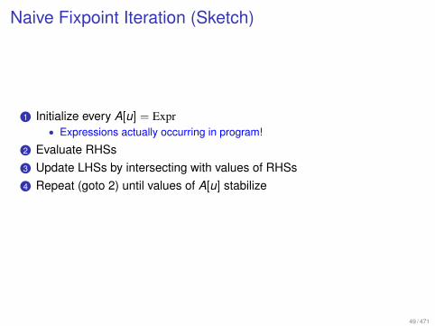
Naive Fixpoint Iteration (Sketch)

1 Initialize every A[u] = Expr• Expressions actually occurring in program!

2 Evaluate RHSs3 Update LHSs by intersecting with values of RHSs4 Repeat (goto 2) until values of A[u] stabilize

49 / 471

Naive Fixpoint Iteration (Example)

• On whiteboard!

50 / 471

Naive Fixpoint Iteration (Correctness)

Why does the algorithm terminate?• In each step, sets get smaller• This can happen at most |Expr| times.

Why does the algorithm compute a solution?• If not arrived at solution yet, violated constraint will cause decrease of LHS

Why does it compute the maximal solution?• Fixed-point theory. (Comes next)

51 / 471




4 Alias Analysis







Partial Orders

Definition (Partial Order)A partial order (D,v) is a relation v on D that is reflexive, antisymmetric, andtransitive, i.e., for all a,b, c ∈ D:

a v a (reflexive)a v b ∧ b v a =⇒ a = b (antisymmetric)

a v b v c =⇒ a v c (transitive)

Examples ≤ on N, ⊆. Also ≥, ⊇

Lemma (Dual order)We define a w b := b v a. Let v be a partial order on D. Then w also is apartial order on D.

53 / 471

More examples

D = 2{a,b,c} with ⊆

{a} {b} {c}

∅

{a,b} {a, c} {b, c}

{a,b, c}

54 / 471

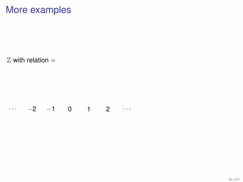
More examples

Z with relation =

. . . −2 −1 0 1 2 . . .

55 / 471

More examples

Z with relation ≤

. . .

−2

−1

0

1

2

. . .

56 / 471

More examples

Z⊥ := Z ∪ {⊥} with relation x v y iff x = ⊥ ∨ x = y

. . . −2 −1 0 1 2 . . .

⊥

57 / 471

More examples

{a,b, c,d} with a @ c,a @ d ,b @ c,b @ d

a b

c d

58 / 471

Upper Bound

Definition (Upper bound)d ∈ D is called upper bound of X ⊆ D, iff

∀x ∈ X . x v d

Definition (Least Upper bound)d ∈ D is called least upper bound of X ⊆ D, iff

d is upper bound of X , andd v y for every upper bound y of X

ObservationUpper bound not always exists, e.g. {0, 2, 4, . . .} ⊆ ZLeast upper bound not always exists, e.g. {a, b} ⊆ {a, b, c, d} witha @ c, a @ d , b @ c, b @ d

59 / 471

Complete Lattice

Definition (Complete Lattice)A complete lattice (D,v) is a partial order where every subset X ⊆ D has aleast upper bound

⊔X ∈ D.

Note Every complete lattice has• A least element ⊥ :=

⊔∅ ∈ D

• A greatest element > :=⊔D ∈ D

Moreover a t b :=⊔{a,b} and a u b :=

d{a,b}

60 / 471

Examples

• (2{a,b,c},⊆) is complete lattice• (Z,=) is not. Nor is (Z,≤)

• (Z⊥,v) is also no complete lattice• But we can define flat complete lattice

61 / 471

Flat complete lattice over Z

Z>⊥ := Z ∪ {⊥,>} with relation x v y iff x = ⊥ ∨ y = > ∨ x = y

. . . −2 −1 0 1 2 . . .

⊥

>

Note This construction works for every set, not only for Z.

62 / 471

Greatest Lower Bound

TheoremLet D be a complete lattice. Then every subset X ⊆ D has a greatest lowerbound

dX.

Proof:• Let L = {l ∈ D. ∀x ∈ X . l v x}

• The set of all lower bounds of X• Construct

dX :=

⊔L

• Show:⊔

L is lower bound• Assume x ∈ X .• Then ∀l ∈ L. l v x (i.e., x is upper bound of L)• Thus

⊔L v x (b/c

⊔L is least upper bound)

• Obvious:⊔

L is w than all lower bounds

63 / 471

Examples

• In (2{a,b,c},⊆)• Note, in lattices with ⊆-ordering, we occasionally write

⋃,⋂

instead of⊔,

d

•⋃{{a, b}, {a, c}} = {a, b, c},

⋂{{a, b}, {a, c}} = {a}

• In Z+∞−∞:•

⊔{1, 2, 3, 4} = 4,

d{1, 2, 3, 4} = 1

•⊔{1, 2, 3, 4, . . .} = +∞,

d{1, 2, 3, 4, . . .} = 1

64 / 471

Last Lecture

• Syntactic criterion for available expressions• Constraint system to express it

• Yet to come: Link between CS and path-based criterion

• Naive fixpoint iteration to compute maximum solution of CS• Partial orders, complete lattices

65 / 471

Monotonic function

DefinitionLet (D1,v1) and (D2,v2) be partial orders. A function f : D1 → D2 is calledmonotonic, iff

∀x , y ∈ D1. x v1 y =⇒ f (x) v2 f (y)

66 / 471

Examples

• f :: N→ Z with f (x) := x − 10• f :: N→ N with f (x) := x + 10• f :: 2{a,b,c} → 2{a,b,c} with f (X ) := (X ∪ {a,b}) \ {b, c}

• In general, functions of this form are monotonic wrt. ⊆.

• f :: Z→ Z with f (x) := −x (Not monotonic)• f :: 2{a,b,c} → 2{a,b,c} with f (X ) := {x | x /∈ X} (Not monotonic)

• Functions involving negation/complement usually not monotonic.

67 / 471

Least fixed point

DefinitionLet f : D→ D be a function.A value d ∈ D with f (d) = d is called fixed point of f .

If D is a partial ordering, a fixed point d0 ∈ D with

∀d . f (d) = d =⇒ d0 v d

is called least fixed point. If such a d0 exists, it is uniquely determined, and wedefine

lfp(f ) := d0

68 / 471

Examples

• f :: N→ N with f (x) = x + 1 No fixed points• f :: N→ N with f (x) = x . Every x ∈ N is fixed point.• f :: 2{a,b,c} → 2{a,b,c} with f (X ) = X ∪ {a,b}. lfp(f ) = {a,b}.

69 / 471

Function composition

TheoremIf f1 : D1 → D2 and f2 : D2 → D3 are monotonic, then also f2 ◦ f1 is monotonic.

Proof: a v b =⇒ f1(a) v f1(b) =⇒ f2(f1(a)) v f2(f1(b)).

70 / 471

Function lattice

DefinitionLet (D,v) be a partial ordering. We overload v to functions from A to D:

f v g iff ∀x . f (x) v g(x)

[A→ D] is the set of functions from A to D.

TheoremIf (D,v) is a partial ordering/complete lattice, then also ([A→ D],v).In particular, we have:

(⊔

F )(x) =⊔{f (x) | f ∈ F}

Proof: On whiteboard.

71 / 471

Component-wise ordering on tuples

• Tuples ~x ∈ Dn can be seen as functions ~x : {1, . . . ,n} → D• Yields component-wise ordering:

~x v ~y iff ∀i : {1, . . . ,n}. xi v yi

• (Dn,v) is complete lattice if (D,v) is complete lattice.

72 / 471

Application• Idea: Encode constraint system as function. Solutions as fixed points.• Constraints have the form

xi w fi (x1, . . . , xn)

where

xi variables e.g., A[u], for u ∈ V(D,v) complete lattice e.g., (2Expr,⊇)

fi : Dn → D RHS e.g., (A[u] ∪ {e}) \ ExprR

• Observation: One constraint per xi is enough.• Assume we have xi w rhs1(x1, . . . , xn), ..., xi w rhsm(x1, . . . , xn)• Replace by xi w (

⊔{rhsj | 1 ≤ j ≤ m})(x1, . . . , xn)

• Does not change solutions.

• Define F : Dn → Dn, with

F (x1, . . . , xn) := (f1(x1, . . . , xn), . . . , fn(x1, . . . , xn))

Then, constraints expressed by ~x w F (~x).• Fixed-Points of F are solutions• Least solution = least fixed point (next!)

73 / 471

Least fixed points of monotonic functions

• Moreover, F is monotonic if the fi are.• Question: Does lfp(F ) exist? Does fp-iteration compute it?

74 / 471

Knaster-Tarski fixed-point TheoremKnaster-TarskiLet (D,v) be a complete lattice, and f : D→ D be a monotonic function.Then, f has a least and a greatest fixed point given by

lfp(f ) =l{x | f (x) v x} gfp(f ) =

⊔{x | x v f (x)}

Proof Let P = {x | f (x) v x}. (P is set of pre-fixpoints)• Show (1): f (

dP) v

dP.

• Have ∀x ∈ P. f (d

P) v f (x) v x (lower bound, mono, def.P)• I.e., f (

dP) is lower bound of P

• Thus f (d

P) vd

P (greatest lower bound).• Show (2):

dP v f (

dP)

• From (1) have f (f (d

P)) v f (d

P) (mono)• Hence f (

dP) ∈ P (def.P)

• Thusd

P v f (d

P) (lower bound).• Show (3): Least fixed point

• Assume d = f (d) is another fixed point• Hence f (d) v d (reflexive)• Hence d ∈ P (def.P)• Thus

dP v d (lower bound)

• Greatest fixed point: Dually.75 / 471

Used Facts

lower bound x ∈ X =⇒d

X v xgreatest lower bound (∀x ∈ X . d v X ) =⇒ d v

dX

mono f monotonic: x v y =⇒ f (x) v f (y)

reflexive x v x

76 / 471

Knaster-Tarski Fixed-Point Theorem (Intuition)

f (x) v x pre-fixpoints

x v f (x) post-fixpoints

x = f (x)

gfp

lfp

77 / 471

Least solution = lfp

Recall: Constraints where ~x w F (~x)

Knaster-Tarski: lfp(F ) =d{~x | ~x w F (~x)}

• I.e.: Least fixed point is lower bound of solutions

78 / 471

Kleene fixed-point theorem

Kleene fixed-point

Let (D,v) be a complete lattice, and f : D→ D be a monotonic function. Then:⊔{f i (⊥) | i ∈ N} v lfp(f )

If f is distributive, we even have:⊔{f i (⊥) | i ∈ N} = lfp(f )

DefinitionDistributivity A function f : D1 → D2 over complete lattices (D1,v1) and(D2,v2) is called distributive, iff

X 6= ∅ =⇒ f (⊔

1X ) =

⊔2{f (x) | x ∈ X}

Note: Distributivity implies monotonicity.

79 / 471

Kleene fixed-point theorem: Proof

By Knaster-Tarski theorem, lfp(f ) exists.Show that for all i : f i (⊥) v lfp(f )• Induction on i.

• i = 0: f 0(⊥) = ⊥ v lfp(f ) (def.f 0, bot least)• i + 1: IH: f i (⊥) v lfp(f ). To show: f i+1(⊥) v lfp(f )• Have f i+1(⊥) = f (f i (⊥)) (def.f i+1)• v f (lfp(f )) (IH, mono)• = lfp(f ) (lfp(f ) is fixed point)

I.e., lfp(f ) is upper bound of {f i (⊥) | i ∈ N}Thus,

⊔{f i (⊥) | i ∈ N} v lfp(f ) (least upper bound)

80 / 471

Kleene fixed-point theorem: Proof (ctd)

Assume f is distributive.Hence f (

⊔{f i (⊥) | i ∈ N}) =

⊔{f i+1(⊥) | i ∈ N} (def.distributive)

=⊔{f i (⊥) | i ∈ N} (

⊔(X ∪ {⊥}) =

⊔X )

I.e.,⊔{f i (⊥) | i ∈ N} is fixed point

Hence lfp(f ) v⊔{f i (⊥) | i ∈ N} (lfp is least fixed point)

With distributive implies mono, antisymmetry and first part, we get:

lfp(f ) =⊔{f i (⊥) | i ∈ N}

81 / 471

Used Facts

bot least ∀x . ⊥ v xfixed point d is fixed point iff f (d) = d

least fixed point f (d) = d =⇒ lfp(f ) v dleast upper bound (∀x ∈ X . x v d) =⇒

⊔X v d

82 / 471

Summary

• Does lfp(F ) exist?• Yes (Knaster-Tarski)

• Does fp-iteration compute it?• Fp-iteration computes the F i (⊥) for increasing i

• By Kleene FP-Theorem, these are below lfp(F )

• It terminates only if a fixed-point has been reached• This fixed point is also below lfp(F ) (and thus = lfp(F ))

83 / 471

Note

• For any monotonic function f , we have

f i (⊥) v f i+1(⊥)

• Straightforward induction on i

84 / 471




4 Alias Analysis







Naive FP-iteration, again

Input Constraint system xi w fi (~x)

1 ~x := (⊥, . . . ,⊥)

2 ~x := F (~x) (Recall F (~x) = (f1(~x), . . . , fn(~x)))3 If ¬(F (~x) v ~x), goto 24 Return “~x is least solution”

Note Originally, we had ~x := ~x t F (~x) in Step 2 and F (~x) 6= ~x inStep 3• Also correct, as F i (⊥) ≤ F i+1(⊥), i.e., ~x v F (~x)• Saves t operation.• v may be more efficient than =.

86 / 471

Caveat

Naive fp-iteration may be rather inefficient

1

2

3

4

5

x := y+z

M[1] := 1

M[2] := 1

M[3] := 1

Let S := (Expr ∪ {y + z}) − Exprx0 1 2 3 4 5

A[1] Expr ∅ ∅ ∅ ∅ ∅A[2] Expr S {y + z} {y + z} {y + z} {y + z}A[3] Expr Expr S {y + z} {y + z} {y + z}A[4] Expr Expr Expr S {y + z} {y + z}A[5] Expr Expr Expr Expr S {y + z}

87 / 471

Round-Robin iteration

Idea: Instead of values from last iteration, use current values whilecomputing RHSs.

1

2

3

4

5

x := y+z

M[1] := 1

M[2] := 1

M[3] := 1

0 1A[1] Expr ∅A[2] Expr {y + z}A[3] Expr {y + z}A[4] Expr {y + z}A[5] Expr {y + z}

88 / 471

RR-Iteration: Pseudocode

~x := (⊥, . . . ,⊥)do {finished := truefor (i=1;i<=n;++i) {new := fi (~x) // Evaluate RHSif (xi 6= new) { // If something changed

finished = false // No fp reached yetxi := xi t new // Update variable

}}

} while (!finished)return ~x

89 / 471

RR-Iteration: Correctness

Prove invariant: ~x v lfp(F )• Initially, (⊥, . . . ,⊥) v lfp(F ) holds (bot-least)• On update:

• We have (1): ~x ′ = ~x(i := xi t fi (~x)). We assume (IH): ~x v lfp(F )• From (1) we get ~x ′ v ~x t F (~x) (def.v on Dn)• From (IH) we get F (~x) v lfp(F ) (mono, fixed-point)• Hence ~x t F (~x) v lfp(F ) (least-upper-bound, IH)• Together: ~x ′ v lfp(F ) (trans)

Moreover, if algorithm terminates, we have ~x = F (~x)• I.e., ~x is a fixed-point.• Invariant: ~x v least fixed point• Thus: ~x = lfp(F )

90 / 471

Used Facts

trans x v y v z =⇒ x v z

91 / 471

RR-Iteration: Improved Algorithm

We can save some operations• Use v instead of = in test• No t on update

~x := (⊥, . . . ,⊥)do {finished := truefor (i=1;i<=n;++i) {new := fi (~x) // Evaluate RHSif (¬(xi w new)) { // If something changed

finished = false // No fp reached yetxi := new // Update variable

}}

} while (!finished)return ~x

92 / 471

RR-Iteration: Improved Algorithm: Correctness

Justification: Invariant ~x v F (~x)• Holds initially: Obvious• On update:

• We have ~x ′ = ~x(i := fi (~x)). We assume (IH): ~x v F (~x)• Hence ~x v ~x ′ v F (~x) (Def.v, IH)• Hence F (~x) v F (~x ′) (mono)• Together ~x ′ v F (~x ′) (trans)

With this invariant, we have• xi = fi (~x) iff xi w fi (~x) (antisym)• xi t fi (~x) = fi (~x) (sup-absorb)

• sup-absorb: x v y =⇒ x t y = y

93 / 471

RR-Iteration: Termination

Definition (Chain)A set C ⊆ D is called chain, iff all elements are mutually comparable:

∀c1, c2 ∈ C. c1 v c2 ∨ c2 v c1

A partial order has finite height, iff every chain is finite. Then, the height h ∈ Nis the maximum cardinality of any chain.

For a domain with finite chain height h, RR-iteration terminates withinO(n2h) RHS-evaluations.• In each iteration of the outer loop, at least one variable increases, or the

algorithm terminates. A variable may only increase h − 1 times.

94 / 471

Last Lecture

• Monotonic functions• Constraint system modeled as function• Least solution is least fixed point

• Knaster-Tarski fp-thm:• lfp of monotonic function exists

• Kleene fp theorem:• Iterative characterization of lfp for distributive functions• Justifies naive fp-iteration

• Round-Robin iteration• Improves on naive iteration by using values of current round• Still depends on variable ordering

95 / 471

Problem:

The efficiency of RR depends on variable ordering

5

4

3

2

1

x := y+z

M[1] := 1

M[2] := 1

M[3] := 1

Let S := (Expr ∪ {y + z})− Exprx0 1 2 3 4 5

A[1] Expr Expr Expr Expr S {y + z}A[2] Expr Expr Expr S {y + z} {y + z}A[3] Expr Expr S {y + z} {y + z} {y + z}A[4] Expr S {y + z} {y + z} {y + z} {y + z}A[5] Expr ∅ ∅ ∅ ∅ ∅

Rule of thumbu before v , if u →∗ vEntry condition before loop body

96 / 471

Worklist algorithm

Problems of RR (remaining)Complete round required to detect terminationIf only one variable changes, everything is re-computedDepends on variable ordering.

Idea of worklist algorithm• Store constraints whose RHS may have changed in a list

97 / 471

Worklist Algorithm: Pseudocode

W = {1...n}~x = (⊥, . . . ,⊥)

while (W != ε) {get an i ∈ W, W = W - {i}

t = fi (~x)if (¬(t v xi )) {

xi = tW = W ∪ {j | fj depends on variable i}

}}

98 / 471

Worklist Algorithm: Example

• On whiteboard

99 / 471

Worklist Algorithm: Correctness

Invariants 1 ~x v F (~x) and ~x v lfpF• Same argument as for RR-iteration

2 ¬(xi w fi (~x)) =⇒ i ∈W• Intuitively: Constraints that are not satisfied are on worklist• Initially, all i in W• On update: Only RHS that depend on updated variable may

change. Exactly these are added to W .If fi does not depend on variable i , the constraint i holds forthe new ~x , so its removal from W is OK.

• If loop terminates: Due to Inv. 2, we have solution. Due toInv. 1, it is least solution.

100 / 471

Worklist Algorithm: TerminationTheoremFor a monotonic CS and a domain with finite height h, the worklist algorithmreturns the least solution and terminates within O(hN) iterations, where N isthe size of the constraint system:

N :=n∑

i=1

1 + |fi | where |fi | := |{i | fi depends on variable i}|

Proof (Sketch):• Number of iterations = Number of elements added to W .• Initially: n elements• Constraint i added if variable its RHS depends on is changed

• Variable may not change more than h times. Constraint depends on |fi | variables.• Thus, no more than

n +n∑

i=1

h|fi | = hN

elements added to worklist.101 / 471

Worklist Algorithm: Problems

• Dependencies of RHS need to be known.• No problem for our application

• Which constraint to select next from worklist?• Requires strategy.

• Various more advanced algorithms exists• Determine dependencies dynamically (Generic solvers)• Only compute solution for subset of the variables (Local solvers)• Even: Local generic solvers

102 / 471

Summary:

• Constraint systems (over complete lattice, monotonic RHSs)• Encode as monotonic function F : Dn → Dn

• (Least) Solution = (least) fixed point

• Knaster-Tarski theorem: A least solution always exists• Solve by fixpoint-iteration (naive, RR, WL)

• Kleene-Theorem justifies naive fixpoint iteration• Similar ideas to justify RR, WL

• Still Missing:• Link between least solution of constraint system, and

Available at u: A[u] =⋂{[[π]]#∅ | π. v0

π−→ u}

103 / 471




4 Alias Analysis







Monotonic Analysis Framework

Given FlowgraphA complete lattice (D,v).An initialization value d0 ∈ DAn abstract effect [[k ]]# : D→ D for edges k• Such that [[k ]]# is monotonic.

Wanted MOP[u] :=⊔{[[π]]#(d0) | π. v0

π−→ u}MOP = Merge over all paths

Method Compute least solution MFP of constraint system

MFP[v0] w d0 (init)

MFP[v ] w [[k ]]#(MFP[u]) for edges k = (u,a, v) (edge)

MFP = Minimal fixed point

105 / 471

Kam, Ullmann

Kam, Ullman, 1975In a monotonic analysis framework, we have

MOP v MFP

• Intuitively: The constraint system’s least solution (MFP) is a correctapproximation to the value defined over all paths reaching the programpoint (MOP).

• In particular: [[π]]#(d0) v MFP[u] for v0π−→ u

106 / 471

Kam, Ullman: Proof

To show MOP v MFP, i.e. (def.MOP, def.v on Dn)

∀u.⊔{[[π]]#d0 | π. v0

π−→ u} v MFP[u]

It suffices to show that MFP[u] is an upper bound. (least-upper-bound)

∀π,u. v0π−→ u =⇒ [[π]]#d0 v MFP[u]

Induction on π.• Base case: π = ε.

• We have u = v0 (empty-path) and [[ε]]#d0 = d0 (empty-eff)• As MFP is solution, the (init)-constraint yields d0 v MFP[v0].

• Step case: π = π′k for edge k = (u, a, v)

• Assume v0π′−−→ u a−→ v and (IH): [[π′]]#d0 v MFP[u].

To show: [[π′k ]]#d0 v MFP[v ]

• Have [[π′k ]]# = [[k ]]#([[π′]]#d0) (eff-comp)• v [[k ]]#(MFP[u]) (IH,mono)• v MFP[v ] ((edge)-constraint, MFP is solution)

107 / 471

Facts

empty-path u ε−→ v ⇐⇒ u = vempty-eff [[ε]]#d = d

eff-comp [[π1π2]]# = [[π2]]# ◦ [[π1]]#

108 / 471

Problem

• Yet another approximation :(• Recall: Abstract effect was already approximation

• Good news:• If the right-hand sides are distributive, we can compute MOP exactly

109 / 471

Theorem of Kildal

Kildal, 1972In a distributive analysis framework (i.e., a monotonic analysis frameworkwhere the [[k ]]# are distributive), where all nodes are reachable, we have

MOP = MFP

110 / 471

Proof

We already know MOP v MFP. To show that also MFP v MOP, it sufficesto show that MOP is a solution of the constraint system.• As MFP is least solution, the proposition follows.

• Recall:

MOP[u] :=⊔

P[u], where P[u] := {[[π]]#(d0) | π. v0π−→ u}

(init) To show: MOP[v0] w d0

• Straightforward (upper-bound, empty-path, empty-eff)

(edge) To show: MOP[v ] w [[k ]]#MOP[u] for edge k = (u,a, v)• Note (*): P[u] not empty, as all nodes reachable• [[k ]]#MOP[u] =

⊔{[[k ]]#([[π]]#d0) | π. v0

π−→ u} (def.MOP, distrib,*)• =

⊔{[[πk ]]#d0 | π. v0

πk−→ v} (def.[[·]]# on paths. k is edge, path-append)• v

⊔{[[π]]#d0 | π. v0

π−→ v} (sup-subset)• = MOP[v ] (def.MOP)

111 / 471

Facts

path-append k = (u,a, v) ∈ E ∧ v0π−→ u ⇐⇒ v0

πk−→ v• Append edge to path

sup-subset X ⊆ Y =⇒⊔

X v⊔

Y

112 / 471

Note

Reachability of all nodes is essential• No paths to unreachable node u, i.e., MOP[u] = ⊥• But edges from other unreachable nodes possible

=⇒ Constraint of form MFP[u] w . . .

Eliminate unreachable nodes before creating CS• E.g. by DFS from start node.

113 / 471

Depth first search (pseudocode)

void dfs (node u) {if u /∈ R {

R := R ∪ {u}for all v with (u,a, v) ∈ E {dfs v}

}}

void find_reachable () {R = {}dfs(v0)// R contains reachable nodes now

}

114 / 471

Summary

Input CFG, distributive/(monotonic) analysis framework• Framework defines domain (D,v), initial value d0 ∈ D and

abstract effects [[·]]# : E → D→ D• For each edge k , [[k ]]# is distributive/(monotonic)

1 Eliminate unreachable nodes2 Put up constraint system3 Solve by worklist-algo, RR-iteration, ...

Output (Safe approximation of) MOP - solution

Note Abstract effects of available expressions are distributive• As all functions of the form: x 7→ (a ∪ x) \ b

115 / 471

Last lecture

• Worklist algorithm: Find least solution with O(hN) RHS-evaluations• h height of domain, N size of constraint system

• Monotonic analysis framework: (D,⊆), d0 ∈ D, [[·]]# (monotonic)• Yields MOP[u] =

⊔{[[π]]#d0 | π. v0

π−→ u}• Theorems of Kam/Ullman and Kildal

• MOP v MFP,• Distributive framework and all nodes reachable: MOP = MFP

• Started with dead-assignment elimination

116 / 471

Summary (II) – How to develop a program optimization

• Optimization = Analysis + Transformation• Create semantic description of analysis result

• Result for each program point• Depends on states reachable at this program point• In general, not computable• Prove transformation correct for (approximations of) this result

• Create syntactic approximation of analysis result• Abstract effect of edges• Yields monotonic/distributive analysis framework

• Compute MFP.• Approximation of semantic result

• Perform transformation based on MFP

117 / 471




4 Alias Analysis







Now: Dead-Assignment Elimination

Example

1: x = y + 2;2: y = 4;3: x = y + 3

Value of x computed in line 1 never usedEquivalent program:

1: nop;2: y = 4;3: x = y + 3

• x is called dead at 1.

119 / 471

Live registers (semantically)

Register x is semantically live at program point u, iff there is an executionto an end node, that depends on the value of x at u:

x ∈ Live[u] ⇐⇒ ∃π, v , ρ, µ, a.

u π−→ v ∧ v ∈ Vend

∧ (ρ, µ) ∈ [[u]]

∧ [[π]](ρ(x := a), µ) 6=X [[π]](ρ, µ)

Where [[u]] := {(ρ, µ) | ∃ρ0, µ0, π. v0π−→ u ∧ [[π]](ρ0, µ0) = (ρ, µ)}

• Intuition: All states reachable at u• Collecting semantics

• (ρ, µ) =X (ρ′, µ′) iff µ = µ′ and ∀x ∈ X . ρ(x) = ρ′(x)• Equal on memory and “interesting” registers X

• x is semantically dead at u, iff it is not live.• No execution depends on the value of x at u.

120 / 471

Transformation: Dead-Assignment Elimination

• Replace assignments/loads to dead registers by Nop• (u, x := ∗, v) 7→ (u,Nop, v) if x dead at v• Obviously correct

• States reachable at end nodes are preserved

• Correct approximation: Less dead variables (= More live variables)

121 / 471

Live registers (syntactic approximation)Register x is live at u (x ∈ L[u]), iff there is a path u π−→ v , v ∈ Vend, suchthat• π does not contain writes to x , and x ∈ X• or π contains a read of x before the first write to x

Abstract effects, propagating live variables backwards over edge

[[Nop]]#L = L

[[Pos(e)]]#L = L ∪ regs(e)

[[Neg(e)]]#L = L ∪ regs(e)

[[x := e]]#L = L \ {x} ∪ regs(e)

[[x := M(e)]]#L = L \ {x} ∪ regs(e)

[[M(e1) := M(e2)]]#L = L ∪ regs(e1) ∪ regs(e2)

Note: distributive.Lift to path (backwards!): [[k1 . . . kn]]# := [[k1]]# ◦ . . . ◦ [[kn]]#

Live at u (MOP): L[u] =⋃{[[π]]#X | ∃v ∈ Vend. u π−→ v}

122 / 471

Example

1

{y}2

{}3

{y}4

{x , y}5

{y}6

{x , y}x=y+2 y=5 x=y+2 M[y]=x x=0

123 / 471

Liveness: Correct approximation

Theorem(Syntactic) liveness is a correct approximation of semantic livenessLive[u] ⊆ L[u]

• Proof: On whiteboard.

124 / 471

Computing L

Use constraint system

L[u] ⊇ X for u ∈ Vend

L[u] ⊇ [[k ]]#L[v ] for edges k = (u,a, v)

Information propagated backwardsDomain: (Reg,⊆)• Reg: The finitely many registers occurring in program.

=⇒ Finite height

• Moreover, the [[k ]]# are distributive

Can compute least solution (MFP)• Worklist algo, RR-iteration, naive fp-iteration

125 / 471

Backwards Analysis FrameworkGiven CFG, Domain: (D,v), init. value: d0 ∈ D, abstract effects:[[·]]# : D→ D, monotonic

MOP[u] :=⊔{[[π]]#d0 | ∃v ∈ Vend. u π−→ v}

MFP is least solution of

MFP[u] w d0 for u ∈ Vend

MFP[u] w [[k ]]#MFP[v ] for edges k = (u, a, v)

• We have:

MOP v MFP

• If the [[k ]]# are distributive, and from every node an end node can bereached:

MOP = MFP

• Proofs:• Analogously to forward case :)

126 / 471

Example: Dead Assignment elimination

while (x>0) {y = y + 1x = x + yx = 1

}

On whiteboard.

127 / 471

Last Lecture

• Monotonic forward/backward framework• Live variables, dead assignment elimination

• x live at u• Semantically: x ∈ Live[u]: Exists execution that depends on value of x at u• Syntactic approximation: x ∈ L[u]: x read before it is overwritten• Correctness proof

• Induction on path, case distinction over edges

128 / 471

Analysis: Classifications

• Forward vs. backwardForward Considers executions reaching a program point

Backwards Considers executions from program point to end• Must vs. May

Must Something is guaranteed to hold, and thus allowsoptimization• On set domain: v=⊇, i.e. t = ∩

May Something may hold, and thus prevents (correct)optimization• On set domain: v=⊆, i.e. t = ∪

• Kill/Gen analysis• Effects have form [[k ]]#X = X u killk t genk• Particular simple class. Distributive by construction.• Bitvector analysis: Kill/Gen on finite set domain.

• Examples:• Available expressions: forward,must,kill-gen• Live variables: backward,may,kill-gen

129 / 471

Dead Assignment Elimination: Problems

Eliminating dead assignments may lead to new dead assignments

1

{}2

{x}{}3

{}4

{x}5

{x , y}x=1 y=x x=1 y=1

In a loop, a variable may keep itself alive

1{x}

2{x}

x=0

x=x+1

130 / 471

Truly live registers

Idea: Consider assignment edge (u, x = e, v).• If x is not semantically live at v , the registers in e need not become live at u• There values influence a register that is dead anyway.

131 / 471

Example

1

{}2

{}3

{}4

{x}5

{x , y}x=1 y=x x=1 y=1

132 / 471

True Liveness vs. repeated liveness

• True liveness detects more dead variables than repeated liveness

Repeated livenessTrue liveness:

1{x}{}

2{x}

x=0

x=x+1

133 / 471

LiveTruly live registers: Abstract effects

[[Nop]]#TL = TL

[[Pos(e)]]#TL = TL ∪ regs(e)

[[Neg(e)]]#TL = TL ∪ regs(e)

[[x := e]]#TL = TL \ {x} ∪ (x ∈ TL?regs(e): ∅)

[[x := M(e)]]#TL = TL \ {x} ∪ (x ∈ TL?regs(e): ∅)

[[M(e1) := e2]]#TL = TL ∪ regs(e1) ∪ regs(e2)

Effects are more complicated. No kill/gen, but still distributive.We have MFP = MOP :)

134 / 471

True Liveness: Correct approximation

TheoremTrue liveness is a correct approximation of semantic liveness Live[u] ⊆ TL[u]

• Proof: On whiteboard.

135 / 471




4 Alias Analysis







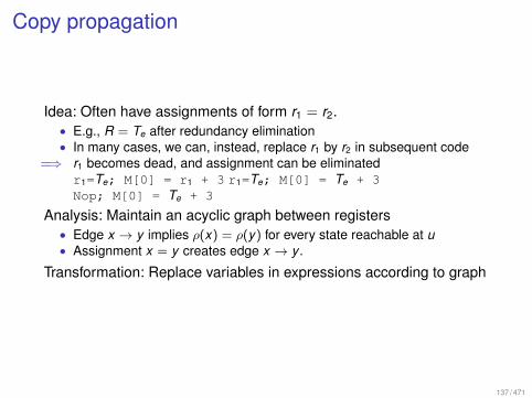
Copy propagation

Idea: Often have assignments of form r1 = r2.• E.g., R = Te after redundancy elimination• In many cases, we can, instead, replace r1 by r2 in subsequent code

=⇒ r1 becomes dead, and assignment can be eliminatedr1=Te; M[0] = r1 + 3 r1=Te; M[0] = Te + 3Nop; M[0] = Te + 3

Analysis: Maintain an acyclic graph between registers• Edge x → y implies ρ(x) = ρ(y) for every state reachable at u• Assignment x = y creates edge x → y .

Transformation: Replace variables in expressions according to graph

137 / 471

Example

On Whiteboard

138 / 471

Abstract Effects

[[Nop]]#C = C

[[Pos(e)]]#C = C

[[Neg(e)]]#C = C

[[x = y ]]#C = C \ {x → ∗, ∗ → x} ∪ {x → y} for y ∈ Reg, y 6= x

[[x = e]]#C = C \ {x → ∗, ∗ → x} for e ∈ Expr \ Reg or e = x

[[x = M[e]]]#C = C \ {x → ∗, ∗ → x}

[[M[e1] = e2]]#C = C

where {x → ∗, ∗ → x} is the set of edges from/to xObviously, abstract effects preserve acyclicity of CMoreover, out-degree of nodes is ≤ 1Abstract effects are distributive

139 / 471

Last Lecture

• Classification of analysis• Forward vs. backward, must vs. may, kill/gen, bitvector

• Truly live variables• Better approximation of „semantically life”• Idea: Don’t care about values of variables that only affect dead variables

anyway.• Copy propagation

• Replace registers by registers with equal value, to create dead assignments

• Whole procedure: Simple redundancy elimination, then CP and DAE toclean up

140 / 471

Analysis Framework

• Domain: (D = 2Reg×Reg,⊇)• I.e.: More precise means more edges (Safe approximation: less edges)• Join: ∩ (Must analysis)• Forward analysis, initial value d0 = ∅

=⇒ MOP[u] =⋂{[[π]]#∅ | v0

π−→ u}• Correctness: x → y ∈ MOP[u] =⇒ ∀(ρ, µ) ∈ [[u]]. ρ(x) = ρ(y)

• Justifies correctness of transformation wrt. MOP• Proof: Later!

• Note: Formally, domain contains all graphs.• Required for complete lattice property!• But not suited for implementation (Set of all pairs of registers)• Add ⊥-element to domain. [[k ]]#⊥ := ⊥.• Intuition: ⊥ means unreachable.

141 / 471




4 Alias Analysis







Procedure as a whole

1 Simple redundancy elimination• Replaces re-computation by memorization• Inserts superfluous moves

2 Copy propagation• Removes superfluous moves• Creates dead assignments

3 Dead assignment elimination

143 / 471

Example: a[7]−−r1=M[a+7]

r2=r1- 1

M[a+7] = r2

Introduced memorization registers

T1 = a+7

r1 = M[T1]

T2 = r1- 1

r2 = T2

T1 = a+7

M[T1]=r2

Eliminated redundant computations

T1 = a+7

r1 = M[T1]

T2 = r1- 1

r2 = T2

Nop

M[T1]=r2

Copy propagation done

T1 = a+7

r1 = M[T1]

T2 = r1- 1

r2 = T2

Nop

M[T1]=T2

Eliminated dead assignments

T1 = a+7

r1 = M[T1]

T2 = r1- 1

Nop

Nop

M[T1]=T2

144 / 471

Table of Contents

1 Introduction



4 Alias Analysis







145 / 471

Background: Simulation

• Given:• Concrete values C, abstract values D, actions A• Initial values c0 ∈ C, d0 ∈ D• Concrete effects [[a]] : C→ C, abstract effects [[a]]# : D→ D

• With forward-generalization to paths: [[k1 . . . kn]] = [[kn]] ◦ . . . ◦ [[k1]] and[[k1 . . . kn]]# = [[kn]]# ◦ . . . ◦ [[k1]]#

• Relation ∆⊆ C× D• Assume:

• Initial values in relation: c0 ∆ d0

• Relation preserved by effects: c ∆ d =⇒ [[k ]]c ∆ [[k ]]#d

• Get: Relation preserved by paths from initial values: [[π]]c0 ∆ [[π]]#d0

• Proof: Straightforward induction on paths. On whiteboard!

146 / 471

Background: Description relation• Now: c ∆ d — Concrete value c described by abstract value d• Moreover, assume complete lattices on C and D.

• Intuition: x v x ′ — x is more precise than x ′

• Assume ∆ to be monotonic on abstract values:

c ∆ d ∧ d v d ′ =⇒ c ∆ d ′

• Intuition: Less precise abstract value still describes concrete value

• Assume ∆ to be distributive on concrete values:

(∀c ∈ C. c ∆ d) ⇐⇒ (⊔

C) ∆ d

• Note: Implies anti-monotonicity: c′ v c ∧ c ∆ d =⇒ c′ ∆ d• Intuition: More precise concrete values still described by abstract value

• We get for all sets of paths P:

(∀π ∈ P. [[π]]c0 ∆ [[π]]#d0) =⇒ (⊔π∈P

[[π]]c0) ∆ (⊔π∈P

[[π]]#d0)

• Intuition: Concrete values due to paths P described by abstract values

147 / 471

Application to Program Analysis

• Concrete values: Sets of states with ⊆• Intuition: Less states = more precise information

• Concrete effects: Effects of edges (generalized to sets of states)• [[k ]]C :=

⋃(ρ,µ)∈C∩dom[[k ]] [[k ]](ρ, µ), i.e., don’t include undefined effects

• Concrete initial values: All states: c0 = State• Abstract values: Domain of analysis, abstract effects: [[k ]]#, d0

• Description relation: States described by abstract value• Usually: Define ∆ on single states, and lift to set of states:

S ∆ A iff ∀(ρ, µ) ∈ S. (ρ, µ) ∆ A

• This guarantees distributivity in concrete states• We get: [[u]] ∆ MOP[u]

• All states reachable at u described by analysis result at u.

148 / 471

Example: Available expressions

• Recall: D = (2Expr,⊇)

• Define: (ρ, µ) ∆ A iff ∀e ∈ A. [[e]]ρ = ρ(Te)

• Prove: A ⊇ A′ ∧ (ρ, µ) ∆ A =⇒ (ρ, µ) ∆ A′

• Prove: (ρ, µ) ∆ A =⇒ [[a]](ρ, µ) = [[tr(a,A)]](ρ, µ)

• where tr(Te = e,A) = if e ∈ A then Nop else Te = e |tr(a,A) = a

• Transformation in CFG: (u, a, v) 7→ (u, tr(a,A[u]), v)

• Prove: ∀ρ0, µ0. (ρ0, µ0) ∆ d0

• For AE, we have d0 = ∅, which implies the above.

• Prove: (ρ, µ) ∈ dom[[k ]] ∧ (ρ, µ) ∆ D =⇒ [[k ]](ρ, µ) ∆ [[k ]]#D• Get: [[u]] ∆ MOP[u], thus [[u]] ∆ MFP[u]

• Which justifies correctness of transformation wrt. MFP

149 / 471

Example: Copy propagation

• (D,v) = (2Reg×Reg,⊇)

• (ρ, µ) ∆ C iff ∀(x → y) ∈ C. ρ(x) = ρ(y)• Monotonic for abstract values.• tr(a,C): Replace variables in expressions due to edges in C• (ρ, µ) ∆ C =⇒ [[a]](ρ, µ) = [[tr(a,C)]](ρ, µ)

• Replace variables by equal variables

• d0 = ∅. Obviously (ρ0, µ0) ∆ ∅ for all ρ0, µ0.

• Show (ρ, µ) ∈ dom[[k ]] ∧ (ρ, µ) ∆ C =⇒ [[k ]](ρ, µ) ∆ [[k ]]#C• Assume (IH) ∀(x → y) ∈ C. ρ(x) = ρ(y)• Assume (1) (ρ′, µ′) = [[k ]](ρ, µ) and (2) x → y ∈ [[k ]]#C• Show ρ′(x) = ρ′(y)• By case distinction on k . On whiteboard.

150 / 471

Table of Contents

1 Introduction


3 Abstract InterpretationConstant PropagationInterval Analysis

4 Alias Analysis







151 / 471

Constant Propagation: Idea

• Compute constant values at compile time• Eliminate unreachable code

y=3

Pos(x-y)>5 Neg(x-y)>5

M[0]=1

y=5

y=y+2

Pos(y<3)

x=y

Neg(y<3)

y=3

Pos(x-3)>5 Neg(x-3)>5

M[0]=1

y=5

y=5

Nop

• Dead-code elimination afterwards to clean up (assume y not interesting)

152 / 471

Approach

• Idea: Store, for each register, whether it is definitely constant at u• Assign each register a value from Z>

. . . −2 −1 0 1 2 . . .

>

• Intuition: >— don’t know value of register

• D = (Reg→ Z>) ∪ {⊥}• Add a bottom-element

• Intuition: ⊥— program point not reachable

• Ordering: Pointwise ordering on functions, ⊥ being the least element.• (D,v) is complete lattice

• Examples• D[u] = ⊥: u not reachable• D[u] = {x 7→ >, y 7→ 5}: y is always 5 at u, nothing known about x

153 / 471

Abstract evaluation of expressions

• For concrete operator � : Z× Z→ Z, we define abstract operator�# : Z> × Z> → Z>:

>�# x := >x �#> := >x �# y := x � y

• Evaluate expression wrt. abstract values and operators:[[e]]# : (Reg→ Z>)→ Z>

[[c]]#D := c for constant c

[[r ]]#D := D(r) for register r

[[e1�e2]]#D := [[e1]]#D�# [[e2]]#D for operator �

Analogously for unary, ternary, etc. operators

154 / 471

Example

• Example: D = {x 7→ >, y 7→ 5}

[[y − 3]]#D = [[y ]]#D −# [[3]]#D

= 5−# 3= 2

[[x + y ]]#D = [[x ]]#D +# [[y ]]#D

= >+# 5= >

155 / 471

Abstract effects (forward)

[[k ]]#⊥ := ⊥ for any edge k

[[Nop]]#D := D

[[Pos(e)]]# :=

{⊥ if [[e]]#D = 0D otherwise

[[Neg(e)]]# :=

{⊥ if [[e]]#D = v , v ∈ Z \ {0}D otherwise

[[r = e]]#D := D(r 7→ [[e]]#D)

[[r = M[e]]]#D := D(r 7→ >)

[[M[e1] = e2]]#D := D

For D 6= ⊥.

Initial value at start: d0 := λx . >.(Reachable, all variables have unknown value)

156 / 471

Last lecture

• Simulation based framework for program analysis• Abstract setting:

• Actions preserve relation ∆ between concrete and abstract state.=⇒ States after executing path are related• Approximation: Complete lattice structure

• ∆ monotonic• Distributive =⇒ generalization to sets of path

• For program analysis:• Concrete state: Sets of program states

• All states reachable via path.

• Constant propagation

157 / 471

Example

1

2

3 4

5

6

7

8

y=3

Pos(x-y)>5 Neg(x-y)>5

M[0]=1

y=5

y=y+2

Pos(y<3)

x=y

Neg(y<3)

D[1] = x 7→ >, y 7→ >D[2] = x 7→ >, y 7→ 3D[3] = x 7→ >, y 7→ 3D[4] = x 7→ >, y 7→ 3D[5] = x 7→ >, y 7→ 3D[6] = x 7→ >, y 7→ 5D[7] = ⊥D[8] = x 7→ >, y 7→ 5

Transformations:Remove (u, a, v) if D[u] = ⊥ or D[v ] = ⊥(u, r = e, v) 7→ (u, r = c, v) if [[e]]#(D[u]) = c ∈ Z

Analogously for test, load, store(u, Pos(c), v) 7→ Nop if c ∈ Z \ {0}(u,Neg(0), v) 7→ Nop

158 / 471

Correctness (Description Relation)

• Establish description relation• Between values, valuations, states

• Values: for v ∈ Z: v ∆ v and v ∆ >• Value described by same value, all values described by >• Note: Monotonic, i.e. v ∆ d ∧ d v d ′ =⇒ v ∆ d ′

• Only cases: d = d ′ or d ′ = > (flat ordering).

• Valuations: For ρ : Reg→ Z, ρ# : Reg→ Z>: ρ ∆ ρ# iff ∀x . ρ(x) ∆ ρ#(x)• Value of each variable must be described.• Note: Monotonic. (Same point-wise definition as for v)

• States: (ρ, µ) ∆ ρ# if ρ ∆ ρ# and ∀s. ¬(s ∆ ⊥)• Bottom describes no states (i.e., empty set of states)• Note: Monotonic. (Only new case: s ∆ ⊥ ∧⊥ v d =⇒ s ∆ d)

159 / 471

Correctness (Abstract values)

• Show: For every constant c and operator �, we have

c ∆ c#

v1 ∆ d1 ∧ v2 ∆ d2 =⇒ (v1� v2) ∆ (d1�# d2)

• We get (by induction on expression)

ρ ∆ ρ# =⇒ [[e]]ρ ∆ [[e]]#ρ#

• Moreover, show ∀ρ0, µ0. (ρ0, µ0) ∆ d0

• Here: ∀ρ0, µ0. (ρ0, µ0) ∆ λx . >⇐= ρ0 ∆ λx . >⇐= ∀x . ρ0(x) ∆ >. Holds by definition.

160 / 471

Correctness (Of Transformations)

• Assume (ρ, µ) ∆ ρ#. Show [[a]](ρ, µ) = [[tr(a, ρ#)]](ρ, µ)• Remove edge if ρ# = ⊥. Trivial.• Replace r = e by r = [[e]]#ρ# if [[e]]#ρ# 6= >

• From ρ ∆ ρ# =⇒ [[e]]ρ ∆ [[e]]#ρ# =⇒ [[e]]ρ = [[e]]#ρ#

• Analogously for expressions in load, store, Neg, Pos.• Replace tests on constants by Nop: Obviously correct.

• Does not depend on analysis result.

161 / 471

Correctness (Steps)

• Assume (ρ′, µ′) = [[k ]](ρ, µ) and (ρ, µ) ∆ C. Show (ρ′, µ′) ∆ [[k ]]#C.• By case distinction on k . Assume ρ# := C 6= ⊥.

• Note: We have ρ ∆ ρ#

• Case k = (u, x = e, v): To show ρ(x := [[e]]ρ) ∆ ρ#(x := [[e]]#ρ#)

⇐= [[e]]ρ ∆ [[e]]#ρ#. Already proved.

• Case k = (u, Pos(e), v) and [[e]]#ρ# = 0:• From [[e]]ρ ∆ [[e]]#ρ#, we have [[e]]ρ = 0• Hence, [[Pos(e)]](ρ, µ) = undefined. Contradiction to assumption.

• Other cases: Analogously.• Our general theory gives us: [[u]] ∆ MFP[u]

• Thus, transformation wrt. MFP is correct.

162 / 471

Constant propagation: Caveat

• Abstract effects are monotonic• Unfortunately: Not distributive

• Consider ρ#1 = {x 7→ 3, y 7→ 2} and ρ#

2 = {x 7→ 2, y 7→ 3}• Have: ρ#

1 t ρ#2 = {x 7→ >, y 7→ >}

• I.e.: [[x = x + y ]]#(ρ#1 t ρ

#2 ) = {x 7→ >, y 7→ >}

• However: [[x = x + y ]]#(ρ#1 ) = {x 7→ 5, y 7→ 2} and

[[x = x + y ]]#(ρ#2 ) = {x 7→ 5, y 7→ 3}

• I.e.: [[x = x + y ]]#(ρ#1 ) t [[x = x + y ]]#(ρ#

2 ) = {x 7→ 5, y 7→ >}• Thus, MFP only approximation of MOP in general.

163 / 471

Undecidability of MOP

• MFP only approximation of MOP• And there is nothing we can do about :(

TheoremFor constant propagation, it is undecidable whether MOP[u](x) = >.

• Proof: By undecidability of Hilbert’s 10th problem

164 / 471

Hilbert’s 10th problem (1900)

• Find an integer solution of a Diophantine equation

p(x1, . . . , xn) = 0

• Where p is a polynomial with integer coefficients.• E.g. p(x1, x2) = x2

1 + 2x1 − x22 + 2

• Solution: (-1,1)• Hard problem. E.g. xn + yn = zn for n > 2. (Fermat’s last Theorem)

• Wiles,Taylor: No solutions.

Theorem (Matiyasevich, 1970)

(Based on work of David, Putnam, Robinson)

It is undecidable whether a Diophantine equation has an integer solution.

165 / 471

Regard the following program

x1=x2=...xn =0while (*) { x1 = x1 + 1 }...while (*) { xn = xn + 1 }r=0if (p(x1,...,xn ) == 0) then r=1u: Nop

• For any valuation of the variables, there is a path through the program• For every path, constant propagation computes the values of the xi

• And gets a precise value for p(x1, . . . , xn)

• r is only found to be non-constant, if p(x1, . . . , xn) = 0• Thus, MOP[u](r) = > if, and only if p(x1, . . . , xn) = 0 has a solution

166 / 471

Extensions

• Also simplify subexpressions:• For {x 7→ >, y 7→ 3}, replace x + 2 ∗ y by x + 6.

• Apply further arithmetic simplifications• E.g. x ∗ 0→ 0, x ∗ 1→ x , . . .

• Exploit equalities in conditions• if (x==4) M[0]=x+1 else M[0]=x →if (x==4) M[0]=5 else M[0]=x

• Use

[[Pos(x == e)]]# =

D if [[x == e]]#D = 1⊥ if [[x == e]]#D = 0D1 otherwise

where D1 := D(x := D(x) u [[e]]#D)• Analogously for Neg(x 6= e)

167 / 471

Table of Contents

1 Introduction


3 Abstract InterpretationConstant PropagationInterval Analysis

4 Alias Analysis







168 / 471

Interval Analysis

• Constant propagation finds constants• But sometimes, we can restrict the value of a variable to an interval, e.g.,

[0..42].

169 / 471

Example

int a[42];for (i=0;i<42;++i) {if (0<=i && i<42)

a[i] = i*2;else

fail();

• Array access with bounds check• From the for-loop, we know i ∈ [0..41]

• Thus, bounds check not necessary

170 / 471

Intervals

Interval I := {[l ,u] | l ∈ Z−∞ ∧ u ∈ Z+∞ ∧ l ≤ u}Ordering ⊆, i.e. [l1,u1] v [l2,u2] iff l1 ≥ l2 ∧ u1 ≤ u2

• Smaller interval contained in larger one• Hence:

[l1,u1] t [l2,u2] = [min(l1, l2),max(u1,u2)]

> = [−∞,+∞]

Problems• Not a complete lattice. (Will add ⊥ - element later)• Infinite ascending chains: [0,0] @ [0,1] @ [0,2] @ . . .

171 / 471

Building the Domain

• Analogously to CP:• D := (Reg→ I) ∪ {⊥}• Intuition: Map variables to intervals their value must be contained in.• ⊥— unreachable

• Description relation:• On values: z ∆ [l, u] iff l ≤ z ≤ u• On register valuations: ρ ∆ ρ# iff ∀x .ρ(x) ∆ ρ#(x)• On configurations: (ρ, µ) ∆ I iff ρ ∆ I and I 6= ⊥• Obviously monotonic. (Larger interval admits more values)

172 / 471

Abstract operators

Constants c# := [c, c]

Addition [l1,u1] +# [l2,u2] := [l1 + l2,u1 + u2]

• Where −∞+ _ := _ +−∞ := −∞,∞+ _ := _ +∞ :=∞Negation −#[l ,u] := [−u,−l]

Multiplication [l1,u1] ∗# [l2,u2] :=[min{l1l2, l1u2,u1l2,u1u2},max{l1l2, l1u2,u1l2,u1u2}]

Division [l1,u1]/#[l2,u2] :=[min{l1l2, l1u2,u1l2,u1u2},max{l1l2, l1u2,u1l2,u1u2}]• If 0 /∈ [l2,u2], otherwise [l1,u1]/#[l2,u2] := >

173 / 471

Examples

• 5# = [5,5]

• [3,∞] +# [−1,2] = [2,∞]

• [−1,3] ∗# [−5,−1] = [−15,5]

• −#[1,5] = [−5,−1]

• [3,5]/#[2,5] = [0,2] (round towards zero)• [1,4]/#[−1,1] = >

174 / 471

Abstract operators

Equality

[l1,u1] ==# [l2,u2] :=

[1,1] if l1 = u1 = l2 = u2

[0,0] if u1 < l2 or l1 > u2

[0,1] otherwise

Less-or-equal

[l1,u1] ≤# [l2,u2] :=

[1,1] if u1 ≤ l2[0,0] if l1 > u2

[0,1] otherwise

Examples• [1,2] ==# [4,5] = [0,0]• [1,2] ==# [−1,1] = [0,1]• [1,2] ≤# [4,5] = [1,1]• [1,2] ≤# [−1,1] = [0,1]

175 / 471

Proof obligations

c ∆ c#

v1 ∆ d1 ∧ v2 ∆ d2 =⇒ v1� v2 ∆ d1�# d2

Analogously for unary, ternary, etc. operators

Then, we get ρ ∆ ρ# =⇒ [[e]]ρ ∆ [[e]]#ρ#

• As for constant propagation

176 / 471

Effects of edges

For ρ# 6= ⊥

[[·]]#⊥ = ⊥

[[Nop]]#ρ# = ρ#

[[x = e]]#ρ# = ρ#(x 7→ [[e]]#

ρ#)

[[x = M[e]]]#ρ# = ρ#(x 7→ >)

[[M[e1] = e2]]#ρ# = ρ#

[[Pos(e)]]#ρ# =

{⊥ if [[e]]#

ρ# = [0,0]

ρ# otherwise

[[Neg(e)]]#ρ# =

{ρ# if [[e]]#

ρ# w [0,0]

⊥ otherwise

177 / 471

Last lecture

• Constant propagation• Idea: Abstract description of values, lift to valuations, states

• Monotonic, but not distributive• MOP solution undecidable (Reduction to Hilbert’s 10th problem)

• Interval analysis• Associate variables with intervals of possible values

178 / 471

Better exploitation of conditions

[[Pos(e)]]#ρ# =

⊥ if [[e]]#ρ# = [0, 0]

ρ#(x 7→ ρ#(x) u [[e1]]#ρ#) if e = x == e1

ρ#(x 7→ ρ#(x) u [−∞, u]) if e = x ≤ e1 and [[e1]]#ρ# = [_, u]

ρ#(x 7→ ρ#(x) u [l,∞]) if e = x ≥ e1 and [[e1]]#ρ# = [l, _]

. . .

ρ# otherwise

[[Neg(e)]]#ρ# =

⊥ if [[e]]#ρ# 6w [0, 0]

ρ#(x 7→ ρ#(x) u [[e1]]#ρ#) if e = x 6= e1

ρ#(x 7→ ρ#(x) u [−∞, u]) if e = x > e1 and [[e1]]#ρ# = [_, u]

ρ#(x 7→ ρ#(x) u [l,∞]) if e = x < e1 and [[e1]]#ρ# = [l, _]

. . .

ρ# otherwise

• where [l1, u1] u [l2, u2] = [max(l1, l2),min(u1, u2)]

• only exists if intervals overlap• this is guaranteed by conditions

179 / 471

Transformations

• Erase nodes u with MOP[u] = ⊥ (unreachable)

• Replace subexpressions e with [[e]]#ρ# = [v , v ] by v (constant

propagation)

• Replace Pos(e) by Nop if [0,0] 6v [[e]]#ρ# (0 cannot occur)

• Replace Neg(e) by Nop if [[e]]#ρ# = [0,0] (Only 0 can occur)

• Yields function tr(k , ρ#)

• Transformation: (u, k , v) 7→ (u, tr(k ,MFP[u]), v)

• Proof obligation:• (ρ, µ) ∆ ρ# =⇒ [[k ]](ρ, µ) = [[tr(k , ρ#)]](ρ, µ)

180 / 471

Example

i=0

Neg(i<42) Pos(i<42)

Neg(0<=i<42) Pos(0<=i<42)

M[a+i]=i*2

i=i+1

⊥{i 7→ >}

⊥{i 7→ [0, 0]} {i 7→ [0, 1]}

⊥ ⊥{i 7→ [0, 0]} {i 7→ [0, 1]}

⊥ ⊥{i 7→ [0, 0]} {i 7→ [0, 1]}

⊥{i 7→ [0, 0]} {i 7→ [0, 1]}

{i 7→ >}

{i 7→ [0, 42]}

{i 7→ [42, 42]} {i 7→ [0, 41]}

⊥ {i 7→ [0, 41]}

{i 7→ [0, 41]}

About 40 iterations later ...181 / 471

Problem

• Interval analysis takes many iterations• May not terminate at all for (i=0;x>0;x--) i=i+1

182 / 471

Widening

• Idea: Accelerate the iteration — at the price of imprecision• Here: Disallow updates of interval bounds in Z.

• A maximal chain: [3, 8] v [−∞, 8] v [−∞,∞]

183 / 471

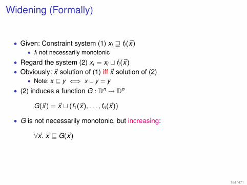
Widening (Formally)

• Given: Constraint system (1) xi w fi (~x)• fi not necessarily monotonic

• Regard the system (2) xi = xi t fi (~x)

• Obviously: ~x solution of (1) iff ~x solution of (2)• Note: x v y ⇐⇒ x t y = y

• (2) induces a function G : Dn → Dn

G(~x) = ~x t (f1(~x), . . . , fn(~x))

• G is not necessarily monotonic, but increasing:

∀~x . ~x v G(~x)

184 / 471

Widening (Formally)

• G is increasing =⇒ ⊥ v G(⊥) v G2(⊥) v . . .• i.e., 〈Gi (⊥)〉i∈N is ascending chain

• If it stabilizes, i.e., ~x = Gk (⊥) = Gk+1(⊥), then ~x is solution of (1)• If D has infinite ascending chains, still no termination guaranteed• Replace t by widening operator t

• Get (3) xi = xi t fi (~x)

• Widening: Any operation D× D→ D1 with x t y v x ty2 and for every sequence a0, a1, . . ., the chain b0 = a0, bi+1 = bi tai+1

eventually stabilizes• Using FP-iteration (naive, RR, worklist) on (3) will

• compute a solution of (1)• terminate

185 / 471

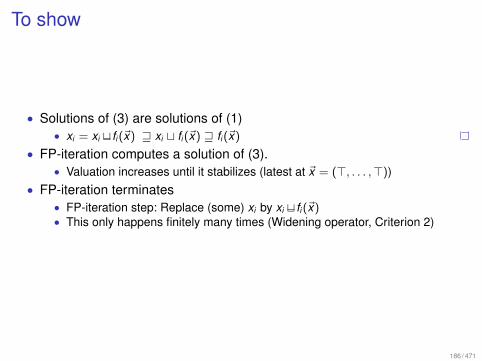
To show

• Solutions of (3) are solutions of (1)• xi = xi t fi (~x) w xi t fi (~x) w fi (~x)

• FP-iteration computes a solution of (3).• Valuation increases until it stabilizes (latest at ~x = (>, . . . ,>))

• FP-iteration terminates• FP-iteration step: Replace (some) xi by xi t fi (~x)• This only happens finitely many times (Widening operator, Criterion 2)

186 / 471

For interval analysis

• Widening defined as [l1,u1]t[l2,u2] := [l ,u] with

l :=

{l1 if l1 ≤ l2−∞ otherwise

u :=

{u1 if u1 ≥ u2

+∞ otherwise

• Lift to valuations: (ρ#1 tρ

#2 )(x) := ρ#

1 (x)tρ#2 (x)

• and to D = (Reg→ I) ∪ {⊥}: ⊥tx = x t⊥ = x• t is widening operator

1 x t y v x ty . Obvious2 Lower and upper bound updated at most once.

• Note: t is not commutative.

187 / 471

Examples

• [−2,2]t[1,2] = [−2,2]

• [1,2]t[−2,2] = [−∞,2]

• [1,2]t[1,3] = [1,+∞]

• Widening returns larger values more quickly

188 / 471

Widening (Intermediate Result)

• Define suitable widening• Solve constraint system (3)• Guaranteed to terminate and return over-approximation of MOP• But: Construction of good widening is black magic

• Even may choose t dynamically during iteration, such that• Values do not get too complicated• Iteration is guaranteed to terminate

189 / 471

Example (Revisited)

i=0

Neg(i<42) Pos(i<42)

Neg(0<=i<42) Pos(0<=i<42)

M[a+i]=i*2

i=i+1

⊥{i 7→ [−∞,+∞]}

⊥{i 7→ [0, 0]} {i 7→ [0,+∞]}

⊥{i 7→ [42,+∞]} ⊥{i 7→ [0, 0]} {i 7→ [0,+∞]}

⊥{i 7→ [42,+∞]} ⊥{i 7→ [0, 0]} {i 7→ [0,+∞]}

⊥{i 7→ [0, 0]} {i 7→ [0,+∞]}

• Not exactly what we expected :(

190 / 471

Idea

• Only apply widening at loop separators• A set S ⊆ V is called loop separator, iff each cycle in the CFG contains a

node from S.• Intuition: Only loops can cause infinite chains of updates.• Thus, FP-iteration still terminates

191 / 471

Problem• How to find suitable loop separator

1

2

3 4

5 6

7

i=0

Neg(i<42) Pos(i<42)

Neg(0<=i<42) Pos(0<=i<42)

M[a+i]=i*2

i=i+1

• We could take S = {2},S = {4}, . . .• Results of FP-iteration are different!

192 / 471

Loop Separator S = {2}1

2

3 4

5 6

7

i=0

Neg(i<42) Pos(i<42)

Neg(0<=i<42) Pos(0<=i<42)

M[a+i]=i*2

i=i+1

⊥{i 7→ [−∞,+∞]}

⊥{i 7→ [0, 0]} {i 7→ [0,+∞]}

⊥{i 7→ [42,+∞]} ⊥{i 7→ [0, 0]} {i 7→ [0, 41]}

⊥ ⊥{i 7→ [0, 0]} {i 7→ [0, 41]}

⊥{i 7→ [0, 0]} {i 7→ [0, 41]}

• Fixed point

193 / 471

Loop Separator S = {4}1

2

3 4

5 6

7

i=0

Neg(i<42) Pos(i<42)

Neg(0<=i<42) Pos(0<=i<42)

M[a+i]=i*2

i=i+1

⊥{i 7→ [−∞,+∞]}

⊥{i 7→ [0, 0]} {i 7→ [0, 1]} {i 7→ [0, 42]}

⊥{i 7→ [42, 42]} ⊥{i 7→ [0, 0]} {i 7→ [0,+∞]}

⊥{i 7→ [42,+∞]} ⊥{i 7→ [0, 0]} {i 7→ [0, 41]}

⊥{i 7→ [0, 0]} {i 7→ [0, 41]}

• Fixed point

194 / 471

Result

• Only S = {2} identifies bounds check as superfluous• Only S = {4} identifies x = 42 at end of program• We could combine the information

• But would be costly in general

195 / 471

Narrowing

• Let ~x be a solution of (1)• I.e., xi w fi (~x)

• Then, for monotonic fi :• ~x w F (~x) w F 2(~x) w . . .

• By straightforward induction

=⇒ Every F k (~x) is a solution of (1)!• Narrowing iteration: Iterate until stabilization

• Or some maximum number of iterations reached• Note: Need not stabilize within finite number of iterations

• Solutions get smaller (more precise) with each iteration• Round robin/Worklist iteration also works!

• Important to have only one constraint per xi !

196 / 471

Example• Start with over-approximation. Stabilized

i=0

Neg(i<42) Pos(i<42)

Neg(0<=i<42) Pos(0<=i<42)

M[a+i]=i*2

i=i+1

{i 7→ [−∞,+∞]}

{i 7→ [0,+∞]}{i 7→ [0, 42]}

{i 7→ [42,+∞]}{i 7→ [42, 42]}{i 7→ [0,+∞]}{i 7→ [0, 41]}

{i 7→ [42,+∞]}⊥ {i 7→ [0,+∞]}{i 7→ [0, 41]}

{i 7→ [0,+∞]}{i 7→ [0, 41]}

197 / 471

Discussion

• Not necessary to find good loop separator• In our example, it even stabilizes

• Otherwise: Limit number of iterations

• Narrowing makes solution more precise in each step• Question: Do we have to accept possible nontermination/large number of

iterations?

198 / 471

Accelerated narrowing

• Let ~x w F (~x) be solution of (1)• Consider function H : ~x 7→ ~x u F (~x)

• For monotonic F , we have ~x w F (~x) w F 2(~x) w . . .• and thus Hk (~x) = F k (~x)

• Now regard I : (~x) 7→ ~x uF (~x), where• u: Narrowing operator, whith

1 x u y v x uy v x2 For every sequence a0, a1, . . ., the (down)chain b0 = a0, bi+1 = bi uai+1

eventually stabilizes• We have: Ik (~x) w Hk (~x) = F k (~x) w F k+1(~x).

• I.e., Ik (~x) greater (valid approx.) than a solution.

199 / 471

For interval analysis

• Preserve (finite) interval bounds: [l1,u1]u[l2,u2] := [l ,u], where

l :=

{l2 if l1 = −∞l1 otherwise

u :=

{u2 if u1 =∞u1 otherwise

• Check:• [l1, u1] u [l2, u2] v [l1, u1]u[l2, u2] v [l1, u1]• Stabilizes after at most two narrowing steps

• u is not commutative• For our example: Same result as non-accelerated narrowing!

200 / 471

Discussion

• Narrowing only works for monotonic functions• Widening worked for all functions

• Accelerated narrowing can be iterated until stabilization• However: Design of good widening/narrowing remains black magic

201 / 471

Last Lecture

• Interval analysis (ctd)• Abstract values: Intervals [l, u] with l ≤ u, l ∈ Z−∞, u ∈ Z+∞

• Abstract operators: Interval arithmetic• Main problem: Infinite ascending chains

• Analysis not guaranteed to terminate• Widening: Accelerate convergence by over-approximating join

• Here: Update interval bounds to −∞/+∞• Problem: makes analysis imprecise

• Idea 1: Widening only at loop separators• Idea 2: Narrowing

• FP-Iteration on solution preserves solution• But may make it smaller

• Accelerated narrowing:• Use narrowing operator for update, that lies “in between” u and original

value• ... and converges within finite time• Here: Keep finite interval bounds

202 / 471

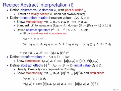
Recipe: Abstract Interpretation (I)• Define abstract value domain A, with partial order v

• t must be totally defined (u need not always exists)• Define description relation between values: ∆⊆ Z× A

• Show: Monotonicity: ∀a1 v a2, v . v ∆ a1 =⇒ v ∆ a2

• Standard: Lift to valuations (Reg→ A), domain (D := (Reg→ A) ∪ {⊥})• Define abstract operators v# : A,�# : A× A→ A, etc.

• Show soundness wrt. concrete ones:

∀c ∈ Z. v ∆ v#

∀v1, v2 ∈ Z, d1, d2 ∈ A. v1 ∆ d1 ∧ v2 ∆ d2 =⇒ v1� v2 ∆ d1�# d2

• For free: ρ ∆ ρ# =⇒ [[e]]ρ ∆ [[e]]#ρ#

• Define transformation tr :: Act× D→ Act• Show correctness: (ρ, µ) ∆ d =⇒ [[a]](ρ, µ) = [[tr(a, d)]](ρ, µ)

• Define abstract effects [[·]]# : Act→ D→ D, initial value d0 ∈ D• Usually: Creativity only required on Pos,Neg• Show: Monotonicity: ∀d1 v d2, a. [[a]]#d1 v [[a]]#d2 and simulation:

∀ρ, µ. (ρ, µ) ∆ d0

∀(ρ, µ) ∈ dom([[a]]), d . (ρ, µ) ∆ d =⇒ [[a]](ρ, µ) ∆ [[a]]#d

203 / 471

Recipe: Abstract Interpretation (II)

• Check finite chain height of domain• Finite: Done• Infinite (or too high)

• Define widening, narrowing operator

204 / 471

Short recapture of methods so far• Operational semantics on flowgraphs

• Edges have effect on states. Extend to paths.• Collecting semantics: [[u]] — States reachable at u.

• Program analysis• Abstract description of

• Forward: States reachable at u• Backward: Executions leaving u

• Abstract effects of edges:• Must be compatible with concrete effects• Forward: Simulation; Backward: Also (kind of) simulation

• MOP[u] — Abstract effects reachable at u• Special case: abstract interpretation — domain describes abstract values

• Transformation: Must be compatible with states/leaving paths describedby abstract effects

• Computing analysis result• Constraint system. For monotonic abstract effects. Precise if distributive.• Solving algorithms: Naive iteration, RR-iteration, worklist algorithm

• Forcing convergence: Widening, Narrowing

205 / 471

Remark: Simulation (Backwards)

• Describe execution to end node (state, path)• Dead variables: Execution does not depend on dead variables

• (ρ, µ), π ∆ D iff ∀x ∈ D, v . [[π]](ρ(x := v), µ) = [[π]](ρ, µ)

• Proof obligations1 (ρ, µ), ε ∆ D0

2 [[a]](ρ, µ), π ∆ D =⇒ (ρ, µ), aπ ∆ [[a]]#D

• Yields: ∀ρ, µ. (ρ, µ), π ∆ [[π]]#D0

• Note: Could even restrict to reachable states ρ, µ.

(ρn, µn), ε

D0

∆

(ρn−1, µn−1),a

D1

[[a]]

[[a]]#

∆

. . .

. . .

(ρ0, µ0), π

Dn

∆

206 / 471

Table of Contents

1 Introduction



4 Alias Analysis







207 / 471

Motivation

• Want to consider memory• E.g. M[y] = 5; x = M[y] + 1 7→ M[y] = 5; x=6

• Here: Assume analyzed program is the only one who accesses memory• In reality: Shared variables (interrupts, threads), DMA, memory-mapped

hardware, ...• Compilers provide, e.g., volatile annotation

208 / 471

First Attempt

• Available expressions:• Memorize loads: Load: x = M[e] 7→ {TM[e] = M[e]; x=TM[e]}• Effects

[[Te = e]]#A = [[A]]# ∪ {e} [[TM[e] = M[e]]]#A = [[A]]# ∪ {M[e]}

[[x = e]]#A = [[A]]# \ Exprx [[M[e1] = e2]]#A = [[A]]# \ loads

. . .

• Problem: Need to be conservative on store• Store destroys all information about memory

209 / 471

Constant propagation

• Apply constant propagation to addresses?• Exact addresses not known at compile time• Usually, different addresses accessed at same program point

• E.g., iterate over array

• Storing at unknown address destroys all information

210 / 471

Last Lecture

• Motivation to consider memory• Alias analysis required!

• Changing the semantics of memory• Pointers to start of blocks, indexing within blocks• No pointer arithmetic• Some assumptions about program correctness: Semantics undefined if

• Program accesses address that has not been allocated• Indexes block out of bounds• Computes with addresses

211 / 471

Extending semantics by blocked memory

• Organize memory into blocks• p = new(e) allocates new block of size e• x = p[e] loads cell e from block p• p[e1] = e2 writes cell e1 from block p

• Semantics• Value: Val = Z ∪ Addr

• Integer values and block addresses• Memory described by µ : Addr ⇀ Z⇀ Val

• Maps addresses of blocks to arrays of values• ⇀ - partial function (Not all addresses/indexes are valid)

• Assumption: Type correct• In reality: Type system

• We write null and 0 synonymously

212 / 471

Semantics

[[Nop]](ρ, µ) = (ρ, µ)

[[x = e]](ρ, µ) = (ρ(x 7→ [[e]]ρ), µ)

[[Pos(e)]](ρ, µ) = [[e]]ρ 6= 0?(ρ, µ) : undefined[[Neg(e)]](ρ, µ) = [[e]]ρ = 0?(ρ, µ) : undefined

[[x = p[e]]](ρ, µ) = (ρ(x 7→ µ([[p]]ρ, [[e]]ρ)), µ)

[[p[e1] = e2]](ρ, µ) = (ρ, µ([[p]]ρ, [[e1]]ρ) 7→ [[e2]]ρ)

[[x = new(e)]](ρ, µ) = (ρ(x 7→ a), µ(a 7→ (i 7→ 0 | 0 ≤ i < [[e]]ρ))) a /∈ dom(µ)

• New initializes the block• Java: OK, C/C++: ???

• Assume that only valid addresses are used• Otherwise, we formally get undefined

• Assume that no arithmetic on addresses is done• Assume infinite supply of addresses

213 / 471

Equivalence

• Note: Semantics does not clearly specify how addresses are allocated• This is irrelevant, consider e.g.

x=new(4); y=new(4) and y=new(4); x=new(4)• Programs should be equivalent• Although memory manager would probably assign different physical

addresses• Two states (ρ, µ) and (ρ′, µ′) are considered equivalent, iff they are

equivalent up to permutation of addresses• We write (ρ, µ) ≡ (ρ′, µ′)

• Note: To avoid this nondeterminism in semantics:• Choose Addr to be totally ordered• Always take the smallest free address

214 / 471

Examples

• Building the linked list [1,2]

p1 = new (2)p2 = new (2)p1[0] = 1p1[1] = p2p2[0] = 2p2[1] = null

p1

p2

1 2null

215 / 471

Examples

• List reversal

R = nullwhile (T != null) {H = TT = T[0]H[0] = RR = H

}

• Sketch algorithm on whiteboard

216 / 471

Alias analysis

• May alias: May two pointers point to the same address• On store: Only destroy information for addresses that may alias with stored

address• Must alias: Must two pointers point to the same address

• If so, store to one can update information for the other• Here: Focus on may-alias

• Important to limit the destructive effect of memory updates• Must alias: Usually only done in local scope, by, e.g., copy propagation

217 / 471

First Idea• Summarize (arbitrarily many) blocks of memory by (fixed number of)

allocation sites• Use start node of edge in CFG to identify allocation site• Abstract values Addr# = V , Val# = 2Addr#

(Possible targets for pointer)• Domain: (Reg→ Val#)× (Addr# → Val#)

• Effects. . .

[[_, x = y, _]]#(R,M) = (R(x 7→ R(y)),M) for y ∈ Reg

[[_, x = e, _]]#(R,M) = (R(x 7→ ∅),M) for e /∈ Reg

[[u, x = new(e), v]]#(R,M) = (R(x 7→ {u}),M)

[[_, x = p[e], _]]#(R,M) = (R(x 7→⋃{M[a] | a ∈ R[p]}),M)

[[_,p[e1] = y, _]]#(R,M) = (R,M(a 7→ M(a) ∪ R(y) | a ∈ R(p))) for y ∈ Reg

[[_,p[e1] = e, _]]#(R,M) = (R,M) for e /∈ Reg

x may point to addresses where y may point to. Expressions are neverpointers. x points to this allocation site. x may point to everything that a maypoint to, for p pointing to a Add addresses from y to each possible address ofp Expressions are never pointers.

218 / 471

Example

u: p1 = new (2)v: p2 = new (2)p1[0] = 1p1[1] = p2p2[0] = 2p2[1] = null

• At end of program, we have

R = p1 7→ {u},p2 7→ {v}M = u 7→ {v}, v 7→ {}

219 / 471

Description Relation

(ρ, µ) ∆ (R,M) iff ∃s : Addr→ V . ∀a,a′ ∈ Addr. ∀x , i .ρ(x) = a =⇒ s(a) ∈ R(x) (1)∧ µ(a, i) = a′ =⇒ s(a′) ∈ M(s(a)) (2)

Intuitively: There is a mapping s from addresses to allocation sites, with:(1) If a register contains an address, its abstract value contains the

corresponding allocation site(2) If a memory block contains an address (at any index), its abstract value

contains the corresponding allocation site

From this, we can extract may-alias information: Pointers p1,p2 may onlyalias (i.e., ρ(p1) = ρ(p2) ∈ Addr), if R(p1) ∩ R(p2) 6= ∅.• B/c if ρ(p1) = ρ(p2) = a ∈ Addr, we have s(a) ∈ R(p1) ∩ R(p2)

Correctness of abstract effects (sketch)• On whiteboard

220 / 471

Discussion

• May-point-to information accumulates for store.• If store is not initialized, we find out nothing

• Analysis can be quite expensive• Abstract representation of memory at each program point• Does not scale to large programs

221 / 471

Flow insensitive analysis

• Idea: Do not consider ordering of statements• Compute information that holds for any program point

• Only one instance of abstract registers/memory needed

• For our simple example: No loss in precision

222 / 471

First attempt

• Each edge (u,a, v) gives rise to constraintsa constraints

x = y R(x) ⊇ R(y)x = new(e) R(x) ⊇ {u}

x = p[e] R(x) ⊇⋃{M(a) | a ∈ R(p)}

p[e1] = x M(a) ⊇ (a ∈ R(p)?R(x) : ∅) for all a ∈ V• Other edges have no effect• Problem: Too many constraints

• O(kn) for k allocation sites and n edges.

• Does not scale to big programs

223 / 471

Last Lecture

• Flow sensitive points-to analysis• Identify blocks in memory with allocation sites• Does not scale. One abstract memory per program point.

• Flow-insensitive points-to analysis• Compute one abstract memory that approximates all program points.• Does not scale. Too many constraints

• Flow-insensitive alias analysis• Compute equivalence classes of p and p[]

224 / 471

Alias analysis

• Idea: Maintain equivalence relation between variables p and memoryaccesses p[]• x ∼ y whenever x and y may contain the same address (at any two program

points)

u: p1 = new (2)v: p2 = new (2)p1[0] = 1p1[1] = p2p2[0] = 2p2[1] = null

• ∼= {{p1[],p2}, {p1}, {p2[]}}

225 / 471

Equivalence relations

• Relation ∼⊆ R × R that is reflexive, transitive, symmetric• Equivalence class [p] := {p′ ∈ R | p ∼ p′}• The equivalence classes partition R. Conversely, any partition of R

defines an equivalence relation.• ∼⊆∼′ (∼ finer than ∼′)

• The set of all equivalence relations on R with ⊆ forms a complete lattice• ∼⊥:= (=)• ∼>:= R × R•

⊔S := (

⋃S)∗

226 / 471

Operations on ERs

• find(~,p): Return equivalence class of p• union(~,p,p’): Return finest ER ∼′ with p ∼′ p′ and ∼⊆∼′

• On partitions of finite sets: Let R = [p1]∼ ∪ . . . ∪ [pn]∼• union(~,p,p’): Let p ∈ [pi ]∼, p′ ∈ [pj ]∼

Result: {[pi ]∼ ∪ [pj ]∼} ∪ {[pk ] | 1 ≤ k ≤ n ∧ k /∈ {i, j}}

227 / 471

Recursive Union

• If x ∼ y , then also x [] ∼ y [] (rec)• After union, we have to add those equivalences!• union*(~,p,p’):

• The finest ER that is coarser than union(~,p,p’) and satisfies (rec)

228 / 471

Alias analysis

π = { {x}, {x[]} | x ∈ Vars } // Finest ER

for (_,a,_) in E do {case a ofx=y: π = union*(π,x,y)

| x=y[e]: π = union*(π,x,y[]) // y variable| y[e]=x: π = union*(π,x,y[]) // y variable

}

• Start with finest ER (=)• Iterate over edges, and union equivalence classes

229 / 471

Example

1: p1 = new (2)2: p2 = new (2)3: p1[0] = 14: p1[1] = p25: p2[0] = 26: p2[1] = null

init {{p1}, {p2}, {p1[]}, {p2[]}}1→ 2 {{p1}, {p2}, {p1[]}, {p2[]}}2→ 3 {{p1}, {p2}, {p1[]}, {p2[]}}3→ 4 {{p1}, {p2}, {p1[]}, {p2[]}}4→ 5 {{p1}, {p2,p1[]}, {p2[]}}5→ 6 {{p1}, {p2,p1[]}, {p2[]}}

230 / 471

Example

1: R = null2: if Neg (T != null) goto 83: H = T4: T = T[0]5: H[0] = R6: R = H7: goto 28:

init {{H}, {R}, {T}, {H[]}, {T []}}3→ 4 {{H,T}, {R}, {H[],T []}}4→ 5 {{H,T ,H[],T []}, {R}}5→ 6 {{H,T ,H[],T [],R}}6→ 7 {{H,T ,H[],T [],R}}

231 / 471

Discussion

• All memory content must have been constructed by analyzed program• p=p[]; p=p[]; q=q[]• What if q points to third element of linked list at p.

=⇒ Only works for whole programs, no input via memory

232 / 471

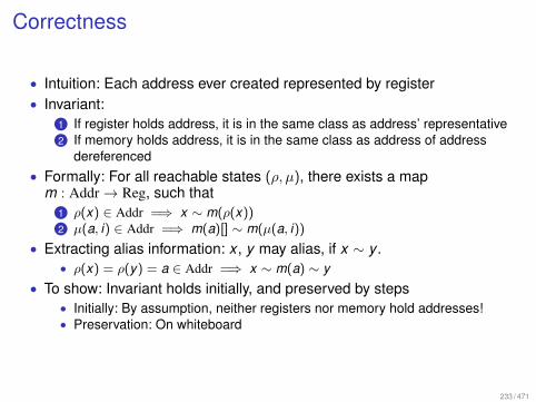
Correctness

• Intuition: Each address ever created represented by register• Invariant:

1 If register holds address, it is in the same class as address’ representative2 If memory holds address, it is in the same class as address of address

dereferenced• Formally: For all reachable states (ρ, µ), there exists a map

m : Addr→ Reg, such that1 ρ(x) ∈ Addr =⇒ x ∼ m(ρ(x))2 µ(a, i) ∈ Addr =⇒ m(a)[] ∼ m(µ(a, i))

• Extracting alias information: x , y may alias, if x ∼ y .• ρ(x) = ρ(y) = a ∈ Addr =⇒ x ∼ m(a) ∼ y

• To show: Invariant holds initially, and preserved by steps• Initially: By assumption, neither registers nor memory hold addresses!• Preservation: On whiteboard

233 / 471

Implementation

• Need to implement union* operation efficiently• Use Union-Find data structure• Equivalence classes identified by unique representative• Operations:

• find(x): Return representative of [x ]• union(x,y): Join equivalence classes represented by x and y

• Destructive update!

234 / 471

Union-Find: Idea• ER represented as forest.• Each node contains element and parent pointer.• Elements of trees are equivalence classes• Representatives are roots of trees• Find: Follow tree upwards• Union: Link root node of one tree to other tree

0 1 2 3 6 74 50 1 2 3 6 74 5

1 1 3 1 4 7 5 7

0

1

3

2

4 7

5

6

235 / 471

Union-Find: Optimizations

• Complexity: Union: O(1), find: O(n) :(• Union by size: Connect root of smaller tree to root of bigger one

• Store size of tree in root node• C - implementation hack: Re/ab-use parent-pointer field for that• Complexity: Union: O(1), find: O(log n) :|

236 / 471

Union by size: Example

0 1 2 3 6 74 50 1 2 3 6 74 5

1 1 3 1 4 7 5 7

0

1

3

2

4 7

5

6

0 1 2 3 6 74 50 1 2 3 6 74 5

0

1

3

2

4

7

1 1 3 1 7 7 5 7

5

6

237 / 471

Path compression

• After find, redirect pointers on path to root node• Requires second pass for find

• Alternative: Connect each node on find-path to its grandfather• Complexity, amortized for m find and n − 1 union operations

• O(n + mα(n))• Where α is the inverse Ackerman-function• Note n < 1080 =⇒ α(n) < 5• Note: This complexity is optimal :)

238 / 471

Path compression: Example

3

4

7

5

2

60

0 1 2 3 6 74 50 1 2 3 6 74 5

5 1 3 1 7 7 5 3

1

3

4

7

5

2

60

0 1 2 3 6 74 50 1 2 3 6 74 5

5 1 3 1 7 7 5 3

1

3

4

7

5

2

60

0 1 2 3 6 74 50 1 2 3 6 74 5

5 1 3 1 7 7 5 3

1

3

4

7

5

2

60

0 1 2 3 6 74 50 1 2 3 6 74 5

5 1 3 1 7 7 5 3

1

3

4

7

5

2

60

0 1 2 3 6 74 50 1 2 3 6 74 5

5 1 3 1 1 7 1 1

1

239 / 471

Placing registers on top

• Try to preserve invariant:• If equivalence class contains register, its representative (root node) is

register• On union, if linking register class to non-register class:

• Swap stored values in roots

• Then, register equivalence class can be identified by its representative

240 / 471

Implementing union*

union*(x,y):x = find(x); y=find(y)if x != y then

union(x,y)if x ∈ Regs & y ∈ Regs then

union*(x[],y[])

241 / 471

Summary

• Complexity:• O(|E |+ |Reg|) calls to union*, find. O(|Reg|) calls to union.

• Analysis is fast. But may be imprecise.• More precise analysis too expensive for compilers.

242 / 471

Last Lecture

• Alias analysis by merging equivalence classes• Implementation by union-find structure

• Optimizations: Union-by-size, path-compression• Implementing union*

243 / 471

Evaluation

Please fill out evaluation forms online.

244 / 471

Table of Contents

1 Introduction



4 Alias Analysis







245 / 471

Table of Contents

1 Introduction



4 Alias Analysis

5 Avoiding Redundancy (Part II)Partial Redundancy EliminationPartially Dead Assignments






246 / 471

Idea

if * {x = M[5]

} else {y1 = x + 1

}y2 = x + 1M[1]=y1 + y2

• x+1 is evaluated on every path• On else-path even two times

247 / 471

Goal

if * {x = M[5]

} else {y1 = x + 1

}y2 = x + 1M[1]=y1 + y2

7→

if * {x = M[5]T=x + 1

} else {T = x + 1y1 = T

}y2=TM[1]=y1 + T

248 / 471

Idea

• Insert assignments Te = e, such that e is available at all program pointswhere it is required.

• Insert assignments as early as possible.• Do not add evaluations of e that would not have been executed at all.

• if x!=0 then y=6 div x 67→ T=6 div x; if x!=0 then y=T

249 / 471

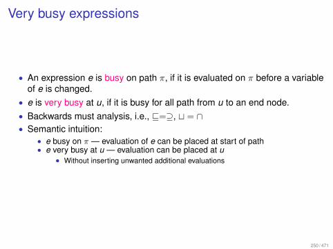
Very busy expressions

• An expression e is busy on path π, if it is evaluated on π before a variableof e is changed.

• e is very busy at u, if it is busy for all path from u to an end node.• Backwards must analysis, i.e., v=⊇, t = ∩• Semantic intuition:

• e busy on π — evaluation of e can be placed at start of path• e very busy at u — evaluation can be placed at u

• Without inserting unwanted additional evaluations

250 / 471

Abstract effects

[[Nop]]#B = B

[[Pos(e)]]#B = B ∪ {e}

[[Neg(e)]]#B = B ∪ {e}

[[x := e]]#B = (B \ Exprx ) ∪ {e}

[[x := M[e]]]#B = (B \ Exprx ) ∪ {e}

[[M[e1] = e2]]#B = B ∪ {e1,e2}

• Initial value: ∅• No very busy expressions at end nodes

• Kill/Gen analysis, i.e., distributive• MOP = MFP, if end node reachable from every node

251 / 471

Example (Very Busy Expressions){}

{}

{x + 1}

{x + 1}

{x + 1}

{x + 1}

{y1 + y2}

{}

x=M[5] y1=x+1

y2=x+1

M[1] = y1+ y2

252 / 471

Available expressions

• Recall: Available expressions before memo-transformation

[[Nop]]#AA := A

[[Pos(e)]]#AA := A ∪ {e}

[[Neg(e)]]#AA := A ∪ {e}

[[R = e]]#AA := (A ∪ {e}) \ ExprR

[[R = M[e]]]#AA := (A ∪ {e}) \ ExprR

[[M[e1] = e2]]#AA := A ∪ {e1,e2}

253 / 471

Transformation

• Insert Te = e after edge (u,a, v), if• e is very busy at v• Evaluation could not have been inserted before, b/c

• e destroyed by a, or• e neither available, nor very busy at u

• Formally: e ∈ B[v ] \ [[a]]#A(A[u] ∪ B[u])

• At program start, insert evaluations of B[v0]• Note: Order does not matter

254 / 471

Transformation

• Place evaluations of expressions• (u, a, v) 7→ {(u, a,w), (w ,Te = e, v)} for e ∈ B[v ] \ [[a]]#

A(A[u] ∪ B[u])• For fresh node w

• v0 7→ v0′ with (v0

′,Te = e, v0) for e ∈ B[v0]

• Note: Multiple memo-assignments on one edge• Can just be expanded in any order

• Replace usages of expressions• (u, x = e, v) 7→ (u, x = Te, v)• analogously for other uses of e

255 / 471

Example• For expression x + 1 only

B = {},A = {}

B = {},A = {}

B = {x + 1},A = {}

B = {x + 1},A = {}

B = {x + 1},A = {x + 1}

B = {x + 1},A = {}

B = {y1 + y2},A = {x + 1}

B = {},A = {x + 1, y1 + y2}

x=M[5] y1=x+1

y2=x+1

M[1] = y1+ y2

T=x+1

y1=x+1y1=Tx=M[5]

T=x+1

y2=x+1y2=T

M[1] = y1+ y2

256 / 471

Correctness (Sketch)• Assumption: Same set of expressions occur at all outgoing edges of a

node• True for our translation scheme• Be careful in general!

=⇒ Required expressions are very busy at start node of edge• Regard path from start node over edge to end node: π1(u,a, v)π2

• Assume expression e required by a• e ∈ B[u]

• Show: On any path π from v0 to v with e ∈ B[v ], evaluation of e is placedsuch that it is available at v

• Induction on π.• Empty path: Evaluation placed before start node• π = π′(u, a, v):

• Case a modifies e =⇒ e /∈ [[a]]#A(. . .) =⇒ Evaluation placed here.

• Case e /∈ A[u] ∪ B[u] =⇒ Evaluation placed here.• Assume: a does not modify e• Case e ∈ B[u]. Induction hypothesis.• Case e ∈ A[u] =⇒ π′ = π′1(u′, a′, v ′)π′2, such that π′2 does not modify e, and e

required by a′ =⇒ e ∈ B[u′]. Induction hypothesis.

257 / 471

Non-degradation of performance

• On any path: Placement of Te = e corresponds to replacing an e by Te

• e not evaluated more often than in original program• Proof sketch: Placement only done where e is very busy

• I.e., every path from placement contains evaluation of e, which will bereplaced

• Moreover, no path contains two evaluations of e, without usage of e inbetween• By contradiction. Sketch on board.

258 / 471

Last Lecture

• Partial Redundancy Elimination• Place evaluations such that

• They are evaluated as early as possible, such that:• Expressions are only evaluated if also evaluated in original program

• Analysis: Very Busy Expressions• Transformation: Placement on edges

• where expression stops to be very busy• or is destroyed (and very busy at target)

• Placement only if expression is not avalable

259 / 471

Application: Moving loop-invariant code

for (i=0;i<N; ++i)a[i] = b + 3

• b+3 evaluated in every iteration.• To the same value• Should be avoided!

260 / 471

Example (CFG)CFG of previous example Analysis results for expression b + 3 Placementhappens inside loop, on edge (2,Pos(i < N),3) :( There is no node outsideloop for placing e!

1: i=0;2: if (i<N) {3: a[i] = b + 34: i=i+15: goto 26: }

1: i=0;2: if (i<N) {3: a[i] = b + 3 // B4: i=i+1 // A5: goto 2 // A6: }

1: i=0;2: if (i<N) {x: T=b+33: a[i] = T4: i=i+15: goto 26: }

261 / 471

Solution: Loop inversion

• Idea: Convert while-loop to do-while loop

while (b) do c 7→if (b) {do c while (b)}

• Does not change semantics• But creates node for placing loop invariant code

262 / 471

ExampleCFG after loop inversion Analysis results for expression b + 3 Placementhappens outside loop, on edge (2,Pos(i < N),3) :)

1: i=0;2: if (i<N) {3: a[i] = b + 34: i=i+15: if (i<N) goto 36: }

1: i=0;2: if (i<N) {3: a[i] = b + 3 // B4: i=i+1 // A5: if (i<N) goto 3 // A6: }

1: i=0;2: if (i<N) {x: T=b+3;3: a[i] = T4: i=i+15: if (i<N) goto 36: }

263 / 471

Conclusion

• PRE may move loop-invariant code out of the loop• Only for do-while loops• To also cover while-loops: Apply loop-inversion first• Loop inversion: No additional statements executed.

• But slight increase in code size.• Side note: Better pipelining behavior (Less jumps executed)

264 / 471

Detecting loops in CFG

• Loop inversion can be done in AST• But only if AST is available• What if some other CFG-based transformations have already been run?

• Need CFG-based detection of loop headers• Idea: Predominators

265 / 471

Predominators

• A node u pre-dominates v (u ⇒ v ), iff every path v0 →∗ v contains u.• ⇒ is a partial order.

• reflexive, transitive, anti-symmetric

266 / 471

Predominator example

1

2

3 4

5

6

1

2

3 4

5

6

267 / 471

Remark: Immediate Predominator

• The⇒-relation, with reflexivity and transitivity removed, is a tree• Clearly, v0 dominates every node (root of tree)• Every node has at most one immediate predecessor:

• Assume u1 ⇒ v , u2 ⇒ v , and neither u1 ⇒ u2 nor u2 ⇒ u1• Regard path π to v . Assume, wlog, π = π1u1π2v , such that u1, u2 /∈ π2• Then, every path π′ to u1 gives rise to path π′π2 to v .• Thus, u2 ∈ π′π2. By asm, not in π2. I.e. u2 ∈ π′.• Thus, u2 ⇒ u1, contradiction.

268 / 471

Computing predominators

• Use a (degenerate) dataflow analysis. Forward, Must. Domain 2V .

• [[(_,_, v)]]#P = P ∪ {v}, d0 = {v0}• Collects nodes on paths• Distributive, i.e. MOP can be precisely computed

• MOP[u] =⋂{[[π]]#{v0} | v0 →∗ u}

• Which is precisely the set of nodes occurring on all paths to u• I.e. the predominators of u

269 / 471

Detecting loops using predominators

• Observation: Entry node of loop predominates all nodes in loop body.• In particular the start node of the back edge

• Loop inversion transformation

v uNeg(e) Pos(e)

if v ∈ P[u]

7→

v

u

Neg(e) Pos(e)

Neg(e) Pos(e)

• Obviously correct

270 / 471

ExampleCFG of running example 2 ∈ P[6], identified pattern for transformationInverted loop

1

2

3 4

5

6

i=0

Neg(i<N) Pos(i<N)

a[i]=b+3

i=i+1

Neg(i<N)Pos(i<N)

271 / 471

Warning

• Transformation fails to invert all loops• E.g., if evaluation of condition is more complex

• E.g., condition contains loads• while (M[0]) ...

1

2

3 4

5

6

x=M[0]

Neg(x) Pos(x)

• We would have to duplicate the load-edge, too

272 / 471

Last Lecture

• Partial redundancy elimination• Very busy expressions• Place evaluations as early as possible

• Loop inversion• while→ do-while• Enables moving loop-invariant code out of loops• Computation on CFG: Use pre-dominators

273 / 471

Table of Contents

1 Introduction



4 Alias Analysis

5 Avoiding Redundancy (Part II)Partial Redundancy EliminationPartially Dead Assignments






274 / 471

Motivation

• Consider program

T = x+1if (*) then M[0]=T

• Assume (*) does not use T , and T dead at end

• Assignment T = x + 1 only required on one path• Would like to move assignment into this path

if (*) then {T = x+1; M[0]=T}

275 / 471

Idea

• Delay assignments as long as possible• Can delay assignment x:=e over edge k , if

• x is not used, nor defined by k• No variable of e is defined by k

276 / 471

Delayable Assignments Analysis

• Domain: {x = e | x ∈ Reg ∧ e ∈ Expr}, Ordering: v=⊇, forward• I.e. forward must analysis

• d0 = ∅, no delayable assignments at program start

[[Nop]]#D = D

[[x = e]]#D = D \ (Ass(e) ∪ Occ(x)) ∪ {x = e}

[[Pos(e)]]#D = D \ Ass(e)

[[Neg(e)]]#D = D \ Ass(e)

[[x = M[e]]]#D = D \ (Ass(e) ∪ Occ(x))

[[M[e1] = e2]]#D = D \ (Ass(e1) ∪ Ass(e2))

where

Ass(e) := {x = e′ | x ∈ Reg(e)} Assignments to variable in e

Occ(x) := {x ′ = e | x = x ′ ∨ x ∈ Reg(e)} Assignments in which x occurs

277 / 471

Intuition

• x = e ∈ D[u]: On every path reaching u, the assignment x = e isexecuted, and no edge afterwards:• Depends on x• Changes x or a variable of e

• Thus, this assignment can be safely moved to u

278 / 471

Transformation• Delay assignments as far as possible• Do not place assignments to dead variables• (u, x = e, v) 7→ (u, ss1,w), (w , ss2, v) where

• ss1 Assignments to live variables that cannot be delayed over action x = e• ss2 Assignments to live variables delayable due to edge, but not at v (Other

paths over v )• w is fresh node• Formally

ss1 := {x ′ = e′ ∈ D[u] \ [[x = e]]#D[u] | x ′ ∈ L[u]}

ss2 = {x ′ = e′ ∈ [[x = e]]#D[u] \ D[v ] | x ′ ∈ L[v ]}

• (u,a, v) 7→ (u, ss1,w1), (w1,a,w2), (w2, ss2, v) for a not assignment

ss1 := {x ′ = e′ ∈ D[u] \ [[a]]#D[u] | x ′ ∈ L[u]}

ss2 = {x ′ = e′ ∈ [[a]]#D[u] \ D[v ] | x ′ ∈ L[v ]}

• ve ∈ Vend 7→ (ve,D[ve], v ′e)• where v ′e is fresh end node, and ve no end node any more.

279 / 471

Dependent actions

• Two actions a1,a2 are independent, iff [[a1a2]] = [[a2a1]]• Actions may be swapped

• Assignments only delayed over independent actions

280 / 471

Correctness (Rough Sketch)

• First: D[u] does never contain dependent assignments• Placement order is irrelevant• Proof sketch: x = e only inserted by [[·]]#, after all dependent assignments

removed

• Regard path with assignment (u, x = e, v).

• We have x = e ∈ [[x = e]]#D[u]. (1) Either placed here, (2) x dead, (3) ordelayable at v• (1) No change of path• (2), not (3): Assignment dropped, but was dead anyway• (3). Three subcases: Sketch on whiteboard!

• (3.1) x = e stops being delayable due to dependent action=⇒ Assignment placed before this action, if live• (3.2) x = e stops being delayable at node

=⇒ Assignment placed after edge to this node, if live• (3.3) x = e delayable until end

=⇒ Assignment placed at end node, if live

281 / 471

Example

1: T = x+1 D: {} L: {x}2: if (*) then { D: {T=x+1} L: {T}3: M[0]=T D: {T=x+1} L: {T}4: Nop D: {} L: {}5: } D: {} L: {}

• Placement of T = x + 1 before edge (3,4)• We have T = x + 1 ∈ D[3] \ [[M[0] = T ]]#D[4], and T ∈ L[3]

1:2: if (*) then {3: T = x+1x: M[0]=T4: Nop5: }

282 / 471

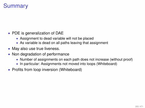
Summary

• PDE is generalization of DAE• Assignment to dead variable will not be placed• As variable is dead on all paths leaving that assignment

• May also use true liveness.• Non degradation of performance

• Number of assignments on each path does not increase (without proof)• In particular: Assignments not moved into loops (Whiteboard)

• Profits from loop inversion (Whiteboard)

283 / 471

Conclusion

• Design of meaningful optimization is nontrivial• Optimizations may only be useful in connection with others• Order of optimization matters• Some optimizations can be iterated

284 / 471

A meaningful ordering

LINV Loop inversionALIAS Alias analysis

AI Constant propagationIntervals

RE (Simple) redundancy eliminationCP Copy propagation

DAE Dead assignment eliminationPRE Partial redundancy eliminationPDE Partially dead assignment elimination

285 / 471

Table of Contents

1 Introduction



4 Alias Analysis







286 / 471

Last Lecture

• Partially dead assignments• Started semantics with procedures

287 / 471

Motivation

• So far:• Only regarded single procedure• But program typically has many procedures• Need to be pessimistic about their effect

• Now:• Analyze effects of procedures• Restrict to procedures without parameters/return values• But with local and global variables!• Can emulate parameters/return values!

288 / 471

Extending the semantics

• Each procedure f represented by control flow graph Gf . Assume theseare distinct!

• Add edge label f () for call of procedure f• Procedure main must exist

Conf = Stack× Globals× StoreGlobals = Glob→ Val

Store = Addr→ ValStack = Frame+

Frame = V × LocalsLocals = Loc→ Val

• where Glob are global variable names, and Loc are local variable names

289 / 471

Execution, small-step semantics

• [[e]](ρl , ρg) : Val. Value of expression.• [[a]](ρl , ρg , µ) : Locals× Globals× Store. Effect of (non-call) action.• Initial configuration: ([(v0

main, λx . 0)], ρg , µ)

• →⊆ Conf× Conf

((u, ρl )σ, ρg , µ)→ ((v , ρ′l )σ, ρ′g , µ′) (basic)

if (u,a, v) ∈ E ∧ [[a]](ρl , ρg , µ) = (ρ′l , ρ′g , µ′)

((u, ρl )σ, ρg , µ)→ ((v0f , λx . 0)(v , ρl )σ, ρg , µ) (call)

if (u, f (), v) ∈ E((u,_)σ, ρg , µ)→ (σ, ρg , µ) (return)

if u ∈ Vend ∧ σ 6= ε

290 / 471

Example (factorial)main():M[0] = fac(3)

fac(x):if (x <= 1) return 1else return x * fac(x-1)

Translation to no arguments and return values

main():m1: Gx = 3;m2: fac()m3: M[0] = Gretm4:

fac():f1: x = Gxf2: if (x <= 1) {f3: Gret = 1

} else {f4: Gx = x-1f5: fac()f6: Gret = x*Gretf7: }

A run:

(m1,−)Gx : −,Gret : −,M[0] : −

(m2,−)Gx : 3,Gret : −,M[0] : −

(f1, x : 0)(m3,−)

Gx : 3,Gret : −,M[0] : −(f2, x : 3)(m3,−)

Gx : 3,Gret : −,M[0] : −(f4, x : 3)(m3,−)

Gx : 3,Gret : −,M[0] : −(f5, x : 3)(m3,−)

Gx : 2,Gret : −,M[0] : −(f1, x : 0)(f6, x : 3)(m3,−)

Gx : 2,Gret : −,M[0] : −(f2, x : 2)(f6, x : 3)(m3,−)

Gx : 2,Gret : −,M[0] : −(f4, x : 2)(f6, x : 3)(m3,−)

Gx : 2,Gret : −,M[0] : −(f5, x : 2)(f6, x : 3)(m3,−)

Gx : 1,Gret : −,M[0] : −(f1, x : 0)(f6, x : 2)(f6, x : 3)(m3,−)

Gx : 1,Gret : −,M[0] : −(f2, x : 1)(f6, x : 2)(f6, x : 3)(m3,−)

Gx : 1,Gret : −,M[0] : −(f3, x : 1)(f6, x : 2)(f6, x : 3)(m3,−)

Gx : 1,Gret : −,M[0] : −(f7, x : 1)(f6, x : 2)(f6, x : 3)(m3,−)

Gx : 1,Gret : 1,M[0] : −(f6, x : 2)(f6, x : 3)(m3,−)

Gx : 1,Gret : 1,M[0] : −(f7, x : 2)(f6, x : 3)(m3,−)

Gx : 1,Gret : 2,M[0] : −(f6, x : 3)(m3,−)

Gx : 1,Gret : 2,M[0] : −(f7, x : 3)(m3,−)

Gx : 1,Gret : 6,M[0] : −(m3,−)

Gx : 1,Gret : 6,M[0] : −(m4,−)

Gx : 1,Gret : 6,M[0] : 6 291 / 471

Realistic Call Semantic

• On real machine, procedure call involves• Save registers• Create stack frame

• Push parameters, return address• Allocate stack space for local variables

• Jump to procedure body• Procedure return

• Free stack frame• Jump to return address• Remove parameters from stack

• Restore registers• Handle result

• Short demo: cdecl calling convention on x86

292 / 471

Inlining• Procedure call is quite expensive• Idea: Copy procedure body to call-site

int f(int a, int b) {int l = a + breturn l + l

}

int g (int a) {return f(a,a)

}

int f(int a, int b) {int l = a + breturn l + l

}

int g (int a) {int l = a + areturn l + l

}293 / 471

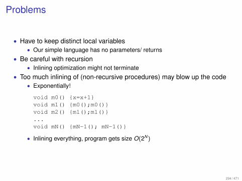
Problems

• Have to keep distinct local variables• Our simple language has no parameters/ returns

• Be careful with recursion• Inlining optimization might not terminate

• Too much inlining of (non-recursive procedures) may blow up the code• Exponentially!

void m0() {x=x+1}void m1() {m0();m0()}void m2() {m1();m1()}...void mN() {mN-1(); mN-1()}

• Inlining everything, program gets size O(2N)

294 / 471

Call Graph

• Graph over procedures• Edge from f to g, if body of f contains call to g• In our examples

main fac g f

• Inline strategies• Leaf: Only leaf procedures• Everything: Every non-recursive procedure• Real compilers use complex heuristics

• Based on code size, register pressure, ...

295 / 471

Inlining transformation

• For edge (u, f (), v)

• Make a copy of Gf , rename locals to fresh names l f1, . . . , lfn

• Replace by edges:• (u, l f = ~0, v f

0) (Initialize locals, goto start node of copy)• (v f

e,Nop, v), for all v fe ∈ V f

end (Link end nodes of copy with v )

u

v

f ()

f:l f = ~0

296 / 471

Tail call optimization

• Idea: If after recursive call, the procedure returns• Re-use the procedure’s stack frame, instead of allocating a new one

void f() {if (Gi < Gn-1) {t = a[Gi]Gi = Gi+1a[Gi]=a[Gi]+tf()

}}

7→

void f() {if (Gi < Gn-1) {

t = a[Gi]Gi = Gi+1a[Gi]=a[Gi]+tt=0; goto f

}}

• Requires no code duplication• Have to re-initialize local variables, according to semantics

• Target for DAE ;)

297 / 471

Tail-Call Transformation

v f0f: u

ve

f() 7→v f

0f: u

ve

l f = ~0

298 / 471

Discussion

• Crucial optimization for languages without loop construct• E.g., functional languages

• No duplication of code or additional local variables• The optimization may also be profitable for non-recursive calls

• Re-use stack-space of current frame for new stack frame• But not expressable in our semantics (Too high-level view on locals)

299 / 471

Interprocedural Analysis

• Want to extend our program analysis to procedures• For example, constant propagation

main() { int t;t = 0;if (t) M[17] = 3;a1 = t;work ();ret = 1 - ret;

}

work() {if (a1) work();ret = a1 ;

}

7→

main() { int t;t = 0;//if (t) M[17] = 3;a1 = 0;work0 ();ret = 1;

}

work0() {//if (a1) work();ret = 0 ;

}

300 / 471

Last Lecture

• Stack-based semantics with procedures• Inlining optimization• Tail-call optimization• Path-based semantics

301 / 471

Generalization of Paths

• Recall: Paths were sequences of actions

path = ε | Act · path

• Now: We can call procedures. A procedure call may• Return on path• Not return on path• Advantageous to make this visible in path structure

slpath = ε | Act · slpath | f (slpath) · slpath

path = ε | Act · path | f (slpath) · path | f< · path

• Intuitively:• f (π): Call to procedure f , which executes π and returns• f<: Call to procedure f , which does not return• slpath: Same level paths, which end on same stack-level as they begin• Note: Inside returning call, all calls must return.

302 / 471

Generalization of Paths• Recall: Paths between nodes

[empty ]−

u ε−→ u[app]

k = (u, a, v) ∈ E v π−→ w

u kπ−−→ w• Now

[empty ]−

u ε−→sl u[app]

k = (u, a, v) ∈ E v π−→sl w

u kπ−−→sl w

[call](u, f (), v) ∈ E v0

f π1−−→sl v fe ∈ Vend v

π2−−→sl w

uf (π1)π2−−−−−→sl w

• And

[emp]−

u ε−→ u[app]

k = (u, a, v) ∈ E v π−→ w

u kπ−−→ w

[call](u, f (), v) ∈ E v0

f π1−−→sl v fe ∈ Vend v

π2−−→ w

uf (π1)π2−−−−−→ w

[ncall](u, f (), v) ∈ E v0

f π−→ w

uf<π−−−→ w

303 / 471

Executions of paths• Recall

[[ε]]s = s [[kπ]]s = [[π]]([[k ]]s)

• Now

[[ε]]s = s [[kπ]]s = [[π]]([[k ]]s)

[[f (π)]]s = H [[π]] s [[f<]]s = enter s

where

enter(ρl , ρg , µ) := (~0, ρg , µ)

combine((ρl , ρg , µ), (ρ′l , ρ′g , µ′)) := (ρl , ρ

′g , µ′)

H e s := combine(s, (e(enter s)))

• Intuition:enter Set up stack frame

combine Combine procedure result with old frame304 / 471

Example

f () {if x>0 then {

x = x - 1f ()x = x + 1

} else {u: Nop

}}

main () {x = 1;f ()x = 0

}

SL-path through main

x=1f(

Pos(x>0)x=x-1f(

Neg(x>0)Nop

)x = x + 1

)x = 0

Path from main to u

x=1f<

Pos(x>0)x=x-1f<

Neg(x>0)

305 / 471

Equivalence of semantics

TheoremThe stack-based and path-based semantics are equivalent:

(∃σ. ([u, ρl ], ρg , µ)→∗ ([v , ρ′l ]σ, ρ′g , µ′))

⇐⇒ (∃π. u π−→ v ∧ [[π]](ρl , ρg , µ) = (ρ′l , ρ′g , µ′))

306 / 471

Proof sketch (Whiteboard)

• Auxiliary lemma: Same-level paths

(([u, ρl ], ρg , µ))→∗ ([v , ρ′l ], ρ′g , µ′)

⇐⇒ (∃π. u π−→sl v ∧ [[π]](ρl , ρg , µ) = (ρ′l , ρ′g , µ′))

• Main ideas ( =⇒ )• Induction on length of execution• Identify non-returning calls:

• Execution in between yields same-level paths (aux-lemma)

• Main ideas (⇐=)• Induction on path structure• Executions can be repeated with stack extended at the bottom

(σ, ρg , µ)→∗ (σ′, ρ′g , µ′) =⇒ (σσ, ρg , µ)→∗ (σ′σ, ρ′g , µ

′)

307 / 471

Abstraction of paths

• Recall: Abstract effects of actions: [[a]]# : D→ D• Actions: Nop, Test, Assign, Load, Store

• Now: Additional actions: Returning/non-returning procedure call• Require: Abstract effects for f (π) and f<

• Define abstract enter#f , combine#

f• H#

f e d = combine#f (d , e(enter#

f (d)))

• [[f (π)]]#d = H#f [[π]]# d

• [[f<]]#d = enter#f (d)

308 / 471

Example: Copy constants

• Simplified constant propagation• Conditions not exploited• Only assignments of form x = y and x = c, c ∈ Z

• Domain: D := Reg→ Z>

• Initially: d0 l := 0, l ∈ Loc, d0 g := >,g ∈ Glob• Abstract effects

[[x := c]]#d = d(x := c) for c ∈ Z

[[x := y ]]#d = d(x := d(y)) for y ∈ Reg

[[x := e]]#d = d(x := >) for e ∈ Expr \ (Z ∪ Reg)

[[x := M(e)]]#d = d(x := >)

[[Pos(e)]]#d = [[Neg(e)]]#d = [[Nop]]#d = [[M(e1) = e2]]#d = d

enter#f d = d(l := 0 | l ∈ Loc)

combine#f d d ′ = λx . x ∈ Loc?d(x) : d ′(x)

309 / 471

Correctness

• Description relation (ρl , ρg , µ) ∆ d• iff ρl ∆ d |Loc and ρg ∆ d |Glob

• Show: ∀ρg , µ. [[π]](~0, ρg , µ) ∆ [[π]]#d0

• By induction on path• Then, case distinction on edges• Generalization of simulation proofs for intraprocedural case

310 / 471

Computing Solutions

• Interested in MOP[u] :=⊔{[[π]]#d0 | v0

main π−→ u}• Idea: Constraint system for same-level effects of functions

S[v0f ] w id (start)

S[v ] w [[k ]]# ◦ S[u] k = (u,a, v) ∈ E (edge)

S[v ] w H#(S[f ]) ◦ S[u] k = (u, f (), v) ∈ E (call)

S[f ] w S[v fe] v f

e ∈ V fend (end)

• And for effects of paths reaching u

R[v0main] w enter# d0 (start)

R[v ] w [[k ]]#R[u] k = (u,a, v) ∈ E (edge)

R[v ] w H#S[f ] R[u] k = (u, f (), v) ∈ E (call)

R[v0f ] w enter#R[u] (u, f (), v) ∈ E (calln)

311 / 471

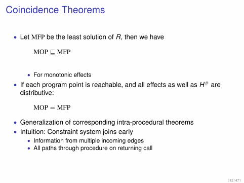
Coincidence Theorems

• Let MFP be the least solution of R, then we have

MOP v MFP

• For monotonic effects

• If each program point is reachable, and all effects as well as H# aredistributive:

MOP = MFP

• Generalization of corresponding intra-procedural theorems• Intuition: Constraint system joins early

• Information from multiple incoming edges• All paths through procedure on returning call

312 / 471

Remaining problem

• How to compute effects of call efficiently?• How to represent functions D→ D• efficiently?

• For copy constants:• Domain is actually finite: Only need to consider constants that actually occur

in the program• But this would yield huge tables for functions

• Possible solutions:• Find efficient representation for functions• Function actually not applied to all values d ∈ D. =⇒ compute on demand.

313 / 471

Efficient representation of same-level effects

• Observation: Functions S[u] 6= ⊥ are of form 〈m〉 where

〈m〉 := λD x . m1 x t⊔

y∈m2 x

D y

• m1 x : Z>⊥ - Join of constants that may be assigned to x• m2 x : 2Reg - set of variables that may be assigned to x (non-empty)

• Let F := {〈m〉|m : Reg→ Z>⊥ × 2Reg} be the set of those functions

• To show: id, [[a]]# ∈ F , and F closed under ◦, t, enter#, and H#

314 / 471

Identity and effects representable

id = 〈λx . (⊥, {x})〉

[[x := e]]# =

〈id(x 7→ (c, ∅))〉 for e = c ∈ Z〈id(x 7→ (⊥, {y}))〉 for e = y ∈ Reg〈id(x 7→ (>, ∅)〉 otherwise

• Effects of other actions similarly

315 / 471

Closed under function composition and join

〈m〉 ◦ 〈m′〉 = 〈λx . (m1 x t⊔

y∈m2 x

m′1 y ,⋃

y∈m2 x

m′2 y)〉

〈m〉 t 〈m′〉 = 〈m tm′〉

• Intuition: Assigned constants by m1, or by m′1, and variable goes throughm2

• [[x := c; foo]]#, or [[x := y ; y := c]]#

• Note: If x not touched, we have m2 x = {x}• Note: t defined pointwise: (m tm′) x = (m1 x tm′1 x ,m2 x ∪m′2 x)

316 / 471

Closed under enter# and H#

enter# = 〈(λx . (0, ∅))|Loc〉 ⊕ id|Glob

H#(〈m〉) = id|Loc ⊕ (〈m〉 ◦ enter#)|Glob

〈m〉|Loc ⊕ 〈m′〉|Glob := 〈λx . x ∈ Loc?m x : m′ x〉

• Intuition• Function call only affects globals• enter# is effect of entering function (set locals to 0)• fLoc ⊕ f ′Glob - Use f for local variables, f ′ for global variables

317 / 471

Recall initial example

main() { int t;t = 0; // t=0, a1=>, ret=>if (t) // t=0, a1=>, ret=>

M[17] = 3; // t=0, a1=>, ret=>a1 = t; // t=0, a1=>, ret=>work (); // t=0, a1=0, ret=>ret = 1 - ret; // t=0, a1=0, ret=0

} // t=0, a1=0, ret=>

work() {if (a1) { // id a1=0, ret=>

work() // id a1=0, ret=>Nop } // id[ ret->(⊥,{a1}) ] a1=0, ret=0

ret = a1 ; // id[ ret->(⊥,{ret,a1}) ] a1=0, ret=>} // id[ ret->(⊥,{a1}) ] a1=0, ret=0

318 / 471

Discussion

• At least copy-constants can be determined interprocedurally• For that, we had to ignore conditions and complex assignments• However, for the reaching paths, we could have been more precise• Extra abstractions were required as

1 Set of abstract same-level effects must be finite2 and efficiently implementable

319 / 471

Last Lecture

• Copy-Constant propagation• Functional approach to interprocedural analysis

• Compute same-level effects by constraint system• Find efficient representation for same-level effects

320 / 471

Idea: Evaluation on demand

• Procedures often called only for few distinct abstract arguments• Observed early (Sharir/Pneuli’81, Cousot’77)

• Only analyze procedures for these• Intuition: [[f ,a]]# - effect of f if called in abstract state a• Put up constraint system

[[v0f , a]]

# w a

[[v , a]]# w [[k ]]#([[u, a]]#) for basic edge k = (u,−, v)

[[v , a]]# w combine#([[u, a]]#, [[g, enter#([[u, a]]#)]]#

) for call edge k = (u, g(), v)

[[f , a]]# w [[v fe, a]]

#for v f

e ∈ V fend

• Idea: Keep track of effect for any node of procedure

321 / 471

Evaluation on demand

• This constraint system may be huge

• Idea: Only evaluate [[f ,a]]# for values a that actually occur• Local fixed-point algorithms (not covered)

• But, we can do an example nevertheless :)

322 / 471

Example: Full constant propagation

// a1,ret | localsmain() { int t;t = 0; >,> | 0if (t) >,> | 0

M[17] = 3; ⊥a1 = t; >,> | 0work (); 0,> | 0ret = 1 - ret; 0,0 | 0

} 0,1 | 0

work() { [[work , (0,>)]]#

if (a1) 0,>work() ⊥

ret = a1 ; 0,>} 0,0

• Only need to keep track of a1 for calling context of work

323 / 471

Discussion

• This analysis terminates, if• D has finite height,• and every procedure only analyzed for finitely many arguments

• Analogous algorithms have proved efficient for analysis of PROLOG• Together with points-to analysis, algorithms of this kind used in the

Goblint-Tool• Data-race detection for C with POSIX-Threads

324 / 471

Crude approximation

• Start with very crude approximation:• Just insert edges from function-call to procedure start• And from return of procedure to target-node of function call

• I.e, for (u, f (), v), generate constraints

D[v0f ] w enter#

f D[u]

D[v ] w combine#f (D[u],D[v f

e]) v fe ∈ V f

end

• Clearly covers all possible paths• But also infeasible ones

325 / 471

Crude approximation, examplef () {...}g () { f() }

main () {f ();g ()

}

main: f:

g:

f()

g()

...

f()

Infeasible paths

326 / 471

Call strings

• Idea: Call string contains sequence of up to k program points• These are the topmost k return addresses on the stack• Analyze procedures for every (feasible) call-string• Only create edges that match call-string

327 / 471

Call strings

D[v0f , (vω)|k ] w enter#(D[u, ω]) (u, f (), v) ∈ E

D[v , ω] w combine#(D[u, ω],D[f , (vω)|k ]) (u, f (), v) ∈ E

D[f , ω] w D[ve, ω] ve ∈ V fend

D[v0main, ε] w d0

D[v , ω] w [[k ]]#D[u, ω] k = (u,a, v) ∈ E

• where ((·)|k ) limits string size to k , cutting off nodes from the end

328 / 471

Example

f () {...}g () { f() }

main () {f ();g ()

}

1main:

2

3

4f2: 5

4’f7: 5’

6g3: 7

f()

g()

...

...

f()

329 / 471

Discussion

• Analysis terminates if D has finite height• Call strings with k = 0 matches crude approximation• Can increase precision by eliminating (some) infeasible paths• Cost increases exponentially with size of k• In practice k = 0 or k = 1• Correctness proof: Simulation wrt. stack-based semantics

330 / 471

Summary: Interprocedural Analysis

• Semantics: Stack-based, path-based• Analysis:

• Functional: Compute same-level effects• Requires efficient representation of effects

• Evaluation on demand: Same-level effects for finite number of arguments• Requires finite/small number of abstract arguments for each function

• Call-Strings: Limit stack-depth, add extra (stack-insensitive) paths abovedepth limit• Adds extra imprecision, exponentially cost in depth-limit

331 / 471

Table of Contents

1 Introduction



4 Alias Analysis







332 / 471

Analysis of Parallel Programs

• Concurrency gets more important nowadays• Admits new classes of bugs

• E.g, data races

• These are hard to find/ hard to reproduce• Can program analysis help?

333 / 471

Data races• Concurrent accesses to global data, one is a write

int g = 0;t1 () {g = g + 1

}main () {fork t1;g = g + 1join;print g

}

• What will the program print?• Assuming sequential consistency?

• Answer: In most cases: 2• But in very rare cases: 1• Depends on machine, other programs, OS, start time, ...

334 / 471

Locks

• Threads can acquire/release locks• Each lock can only be acquired by one thread at the same time• Other threads that want to acquire the lock have to wait• Used to prevent data races

int g = 0; lock lg;t1 () {acquire(lg); g = g + 1; release(lg);

}main () {fork t1;acquire(lg); g = g + 1; release(lg);join;print g

}

335 / 471

Demo: Goblint data race analyzer

• Program with data race• Try to show bad reproducibility + dependence on machine load, etc.• Show goblint-analyzer to find the race

http://goblint.in.tum.de

336 / 471

http://goblint.in.tum.de

Abstract semantics with locks

• We will regard an abstract semantics with locks• I.e., it contains no state beyond the current program points and status of

locks• Concrete program mapped to this semantics

• E.g., pointer analysis to identify locks

• Has more possible executions than concrete program• Analysis results are safe

• If we find no datarace, there is none• But there may be false positives

337 / 471

Parallel flowgraphs with fork

• Add fork(v) edge label, that forks new thread starting at v• For now, we ignore joins!

• Abstract semantics: State is multiset of nodes.• Initial state: {v0}

({u} ∪ s)→ ({v} ∪ s) (u, a, v) ∈ E

({u} ∪ s)→ ({v ,w} ∪ s) (u, fork(w), v) ∈ E

338 / 471

Parallel flowgraphs with fork and locks

• Additionally: Finite set of locks L, actions acq(l) and rel(l)• State: Each thread together with its acquired locks• Initial state: {(v0, ∅)}

({(u,L)} ∪ s)→ ({(v ,L)} ∪ s) (u,a, v) ∈ E({(u,L)} ∪ s)→ ({(v ,L), (w , ∅)} ∪ s) (u, fork(w), v) ∈ E

({(u,L)} ∪ s)→ ({(v ,L ∪ {l})} ∪ s) (u, acq(l), v) ∈ E and l /∈ s|2({(u,L)} ∪ s)→ ({(v ,L \ {l}} ∪ s) (u, rel(l), v) ∈ E

• Note: We assume that a thread only releases locks that it possesses.• We assume that a thread does not acquire a lock it already possesses.• Invariant: For each reachable state, the thread’s lock-sets are disjoint

{(v0, ∅)} →∗ {(u1,L1), (u2,L2)} ∪ s =⇒ L1 ∩ L2 = ∅

339 / 471

Analysis Plan

• Lock-insensitive may-happen in parallel (MHP)• Sets of program points that may be executed in parallel

• Lock-sets• Sets of locks that must be allocated at program point• Used to make MHP more precise

• MHP(u, v) only if u and v have disjoint lock sets

• Data-Races• Identify conflicting program points, with outgoing actions that read/write the

same global variable• Check whether they may happen in parallel

340 / 471

Lock-insensitive MHP• Put up constraint system, R[u]: Set of (interesting) nodes reachable from

u• Reachable also over forks

R[u] ⊇ {u} if u interesting (R.node)R[u] ⊇ R[v ] if (u,_, v) ∈ E (R.edge)R[u] ⊇ R[w ] if (u, fork(w),_) ∈ E (R.trans)

MHP[v ] ⊇ MHP[u] if (u,_, v) ∈ E (MHP.edge)MHP[w ] ⊇ MHP[u] if (u, fork(w), v) ∈ E (MHP.trans)MHP[v ] ⊇ R[w ] if (u, fork(w), v) ∈ E (MHP.fork1)MHP[w ] ⊇ R[v ] if (u, fork(w), v) ∈ E (MHP.fork2)

(R.node) Interesting node reachable from itself (R.edge) Propagatereachability over edge (R.trans) Propagate reachability over fork (MHP.edge)If this edge executed, other threads still at same positions (MHP.trans) Startnode of forked thread parallel to other threads (MHP.fork1) Forking threadparallel to everything that may be reached from forked thread (MHP.fork2)Forked thread parallel to everything that may be reached from forking thread

341 / 471

Correctness

• For interesting nodes u and v (also u=v ), we have:

∃s. {v0} →∗ {u, v} ∪ s =⇒ u ∈ MHP[v ]

• Proof sketch• Auxiliary: {u} →∗ {v} ∪ s =⇒ v ∈ R[u]• Find the crucial fork, where u is reached from, wlog, the forked thread, and v

is reached from the forking thread• {v0} →∗ {a} ∪ . . ., and (a, fork(c), b) ∈ E , and {b} →∗ {u} ∪ . . ., and{c} →∗ {v} ∪ . . .

342 / 471

Lock-set analysis

• Forward, must analysis (standard)

LS[v0] ⊆ ∅LS[w ] ⊆ ∅ (u, fork(w), v) ∈ ELS[v ] ⊆ LS[u] (u,a, v) ∈ E , a no lock-actionLS[v ] ⊆ LS[u] ∪ {l} (u, acq(l), v) ∈ ELS[v ] ⊆ LS[u] \ {l} (u, rel(l), v) ∈ E

• Correctness:

l ∈ LS[u] =⇒ (∀s. {(v0, ∅)} →∗ {(u,L)} ∪ s =⇒ l ∈ L)

343 / 471

Data-Race analysis

• Interesting nodes:• Nodes with actions that read or write global variables

• For each pair (u, v) of conflicting nodes, checku ∈ MHP[v ] =⇒ LS[u] ∩ LS[v ] 6= ∅

• If satisfied, report „definitely no data race”• Otherwise, report possible data race

344 / 471

Exampleint g = 0; lock lg;t1 () {

1: acquire(lg); R: 2 MHP: {7,11} L: {}2: g = g + 1; R: 2 MHP: {7,11} L: {lg}3: release(lg); R: {} MHP: {7,11} L: {lg}4: } MHP: {7,11} L: {}

main () {5: fork t1; R: 2,7,11 MHP: {} L: {}6: acquire(lg); R: 7,11 MHP: {2} L: {}7: g = g + 1; R: 7,11 MHP: {2} L: {lg}8: release(lg); R: 11 MHP: {2} L: {lg}9: join; R: 11 MHP: {2} L: {}10: acquire(lg); R: 11 MHP: {2} L: {}11: print g R: 11 MHP: {2} L: {lg}12: release(lg); R: {} MHP: {2} L: {lg}13: } R: {} MHP: {2} L: {}

• Check lock-sets for 2/7 and 2/11• Lock lg contained in all of them• Program is safe!

345 / 471

Discussion

• Simple (and relatively cheap) analysis• Can prove programs data-race free• But may return false positives, due to:

• Not handling joins• Ignoring data completely• Not handling interaction of locks and control flow

• Fork inside lock• Deadlocks

• Goblint:• Interprocedural• Pointer-analysis• Constant propagation• Equality/inequality of indexes• ...

346 / 471

Discussion

• Freedom of data races often not enough

int x[N];void norm() {

lock l; n = length(x); unlock l;lock l; x = 1/n * x; unlock l;

}

• Thread-safe? No!=⇒ Transactionality

• Advanced locking patterns• E.g., lock chains:

lock 1; lock 2; unlock 1; lock 3; unlock 2 ...

• Two lock-chains executed simultaneously will never overtake

347 / 471

Last Lecture

• Analysis of parallel programs• Intraprocedural with thread creation• May-happen in parallel + lockset analysis = datarace analysis

• Caveats• Need to abstract program into model with fixed locks

• Problematic if locks are addressed via pointers/arrays• Datarace freedom may no be enough

• Transactions• Advanced locking patterns like lockchains

348 / 471

Table of Contents

1 Introduction



4 Alias Analysis







349 / 471

Table of Contents

1 Introduction



4 Alias Analysis




8 Replacing Expensive by Cheaper OperationsStrength ReductionPeephole OptimizationLinearization



350 / 471

Motivating Example

for (i=l;i<r;i=i+h) {a=a0 + b*iM[a] = ...

}

• Initialize array in range: [l , r [, every hth element• Element size of array: b• Loop requires r − l multiplications• Multiplications are expensive, addition much cheaper• Observation: From one iteration of the loop to the next:

• Difference between as is constant: (a0 + b(i + h))− (a0 + bi) = bh

351 / 471

Optimization• First, loop inversion• Second, pre-compute difference and replace computation of a

• No multiplication left in loop• If

• i not used elsewhere in the loop, and• i dead after loop• b not zero• Get rid of i altogether

i=l;if (i<r) {do {

a=a0 + b*iM[a] = ...i=i+h

} while (i<r)}

i=l;if (i<r) {

delta = b*ha=a0 + b*ido {M[a] = ...i=i+ha=a+delta

} while (i<r)}

if (l<r) {delta = b*ha=a0 + b*lN = a0 + b*rdo {

M[a] = ...a=a+delta

} while (a<N)}

352 / 471

In general

• Identify• loops• iteration variables• constants• Matching use structures

353 / 471

Loops

• Identify loop by node v where back-edge leads to, i.e., (u,a, v) ∈ E withv ⇒ u

• Nodes of loop:

loop[v ] = {w | w →∗ v ∧ v ⇒ w}

• I.e., nodes which can only be reached via v , and from which v can bereached again

354 / 471

Example

1

2

3

4

5

6

355 / 471

Iteration variable

• Variable i , such that• All assignments to i in loop have form i := i + h

• where h is loop constant

• Loop constant: Plain constant, or, more sophisticated:• Expression that does not depend on variables modified in loop

• Heuristics for application:• There is an assignment to i in loop• Assignment to i executed in every iteration

356 / 471

Strength reduction

• Strength reduction possible for expressions of the form a0 + b ∗ i , suchthat• a0, b are loop constants• i is iteration variable with increment h

• Introduce temporary variables a and ∆

• Initialize a = a0 + b ∗ i and ∆ = b ∗ h right before loop• Note: Loop must be inverted, to avoid extra evaluations!

• Add a = a + ∆ after assignments to i• Replace expression a0 + b ∗ i by a

357 / 471

Excursus: Floyd-Style verification• Establish invariants for CFG-nodes: Iu for all u ∈ V• Invariant is set of states

• Equivalent notation: Characteristic formula over variables/memory• E.g., a = a0 + b ∗ i describes {(ρ, µ) | ρ(a) = ρ(a0) + b ∗ ρ(i)}

• Show:• (ρ0, µ0) ∈ Iv0

• for states (ρ0, µ0) that satisfy precondition (Here: all states)• For all edges (u, a, v), we have

(ρ, µ) ∈ Iu ∩ dom([[a]]) =⇒ [[a]](ρ, µ) ∈ Iv

• Then, we have, for all nodes u: [[u]] ⊆ Iu• Proof: Induction on paths.

• Recall [[u]] := {(ρ, µ) | ∃ρ0, µ0, π. v0π−→ u ∧ [[π]](ρ0, µ0) = (ρ, µ)}

• Intuition: All states reachable at u• Collecting semantics

• And can use this fact to• Show correctness of program• Justify transformations• ...

358 / 471

Correctness

• Prove that a = a0 + b ∗ i ∧∆ = b ∗ h is invariant for all nodes in loop• Except the target nodes of assignments to i

• There, we have a = a0 + b ∗ (i − h) ∧∆ = b ∗ h

• Proof:• Entering loop: Have put initialization right before loop!• Edge inside loop:

• No assignments to ∆, b, and h• Assignment i := i + h: Check a = a0 + b ∗ i =⇒ a = a0 + b ∗ (i + h − h).• Assignment a := a + ∆. Only occurs directly after assignment to i .

Check a = a0 + b ∗ (i − h) ∧∆ = b ∗ h =⇒ a + ∆ = a0 + b ∗ i• Other edges: Do not modify variables in invariant

359 / 471

Table of Contents

1 Introduction



4 Alias Analysis







360 / 471

Peephole Optimization

• Idea: Slide a small window over the code• Optimize aggressively inside this window• Examples:

x = x ∗ 2 → x = x + xx = x + 1 → x + +

x = 5 + a− a → x = 5x = x → Nopx = 0 → x = x ⊕ x

361 / 471

Sub-Problem: Elimination of Nop

• For edge (u,Nop, v), such that u has no further outgoing edges• Identify u and v• Attention: Do not collapse Nop-loops

• Implementation1 For each node:

• Follow chain of Nop-edges. (Check for loop)• Then redirect all edges on this chain to its end

2 For each edge (u, a, v) with (v ,Nop,w) and v no other outgoing nodes:Replace by (u, a,w)

• Complexity: Linear, O(|E |)1 No edge redirected twice.

(For each newly discovered edge, at most one more edge followed)2 For each edge, only one more edge followed

362 / 471

Table of Contents

1 Introduction



4 Alias Analysis







363 / 471

Motivation• Translate CFG to instruction list• Need to insert jumps. No unique translation.• Crucial for performance

while (b) {...if (b1) {

c1;break;

}...

}

11

22

33

46

57

64

75

b¬b

. . .

¬b1

. . .

b1

c1

1: jneg b 5...jneg b1 6c1

5: halt6: ...

jmp 1

1: jneg b 7...jpos b1 6...jmp 1

6: c17: halt

Bad linearization, jump in loop Good linearization, jump out of loop364 / 471

Heuristics

• Avoid jumps inside loops• Assign each node its loop nesting depth (temperature)

• Hotter nodes are in inner loops

• If jump needs to be inserted: Jump to colder node (out of loop)

365 / 471

Implementation

1 Compute temperatures• Compute predominators• Identify back edges• For each loop head v (i.e., (u, _, v) is back edge)

• Increase temperature of nodes in loop[v ]• Recall:

loop[v ] = {w | w →∗ v ∧ v ⇒ w}

2 Linearize• Pre-order DFS to number nodes• Visit hotter successors first

366 / 471

Example

11

21

31

41

51

60

70

b¬b

. . .

¬b1

. . .

b1

c1

367 / 471

Table of Contents

1 Introduction



4 Alias Analysis







368 / 471

Motivation

• Program needs to be compiled to specific hardware• Which has some features that can be exploited for optimization, e.g.

• Registers• Pipelines• Caches• Multiple Processors

369 / 471

Table of Contents

1 Introduction



4 Alias Analysis





9 Exploiting Hardware FeaturesRegister AllocationSingle Static Assignment FormExploiting Instruction Level ParallelismImproving Memory/Cache Behaviour


370 / 471

Nomenclature

• Variables Var, e.g. x , y , z, . . .: Variables in source program (formerly alsocalled registers)

• Registers Reg, e.g. R1,R2, . . .: Registers after register allocation

371 / 471

Motivation

• Processor only has limited number of registers• Variables need to be mapped to those registers• If no more registers free: Spill to memory

• Expensive!

• Want to map as much variables as possible to registers

372 / 471

Example1: x=M[a]2: y=x+13: if (y=0) {4: z=x*x5: M[a]=z

} else {7: t=-y*y8: M[a]=t9: }

1: R1=M[R3]2: R2=R1+13: if (R2=0) {4: R1=R1*R15: M[R3]=R1

} else {7: R1=-R2*R28: M[R3]=R19: }

• How many registers are needed?Assuming all variables dead at 9

• Variables: a, x , y , z, t .• Three registers suffice:

x , z, t 7→ R1, y 7→ R2, a 7→ R3

373 / 471

Live Ranges

• Live range of variable x : L[x ] := {u | x ∈ L[u]}• Set of nodes where x is alive:• Analogously: True live range

• Observation: Two variables can be mapped to same register, if their liveranges do not overlap

374 / 471

Example

// L a x y z t1: x=M[a] // {a} 12: y=x+1 // {a,x} 1 13: if (y=0) { // {a,x,y} 1 1 14: z=x*x // {a,x} 1 15: M[a]=z // {a,z} 1 1

} else {7: t=-y*y // {a,y} 1 18: M[a]=t // {a,t} 1 19: } // {}

375 / 471

Interference graph

• I = (Var,EI), with (x , y) ∈ Ei iff x 6= y and L[x ] ∩ L[y ] 6= ∅• Graph over variables. Edge iff live ranges overlap.• I is called interference graph

• In our example:x y

z t

a

376 / 471

Last lecture

• Peephole optimization, removal of NOP-edges• Linearization

• Temperature of nodes = loop nesting depth• Preferably jump to colder nodes

• Register allocation• Minimal coloring of interference graph

• NP-hard

377 / 471

Background: Minimal graph coloring

• Given: Graph (V ,E)

• Find coloring of nodes c : V → N, such that• (u, v) ∈ E =⇒ c(u) 6= c(v)

• I.e., adjacent nodes have different colors

• max{c(v) | v ∈ V} is minimal

• Example:1 2

1 1

3

378 / 471

Complexity

• Finding a minimum graph coloring is hard• Precisely: NP-complete to determine whether there is a coloring with at most

k colors, for k > 2.

• Need heuristics

379 / 471

Greedy Heuristics

• Iterate over nodes, and assign minimum color different from alreadycolored neighbors

• Can be implemented using DFS• In theory, result may be arbitrarily far from optimum

• Regard crown graph Cn, which is a complete bipartite graph over 2n nodes,with a perfect matching removed.

• Cn = (ai , bi | i ∈ 1 . . . n, (ai , bj ) | i 6= j)• Minimal coloring uses two colors: One for the as, and one for the bs• Greedy coloring with order a1, b1, a2, b2, . . . uses n colors

• Node ordering heuristics• Nodes of high degree first• Here: Pre-order DFS

380 / 471

Greedy heuristics, pseudocode

color(u):n = { v | (u,v) in E }c(u) = min i. i>=0 and forall v in n. i != c(v)for v in n

if (c(v)==-1) color(v)

main:for u in V do c(u) = -1;

for u in V doif c(u)==-1 then color(u)

381 / 471

Live Range Splitting• Consider basic block,

• i.e., sequence of statements, no jumps in/from in between• (u, a1, v1), (v1, a2, v2), . . . , (vn−1, an, v), with no other edges touching the vi .

• Example:

x=M[0] //y=M[1] // xt=x+y // xyM[2]=t // tx=M[4] //z=M[5] // xt=x+z // x zM[6]=t // ty=M[7] //z=M[8] // yt=y+z // yzM[9]=t // t

x y

z t

• Requires 3 registers• But can do same program with two registers!

382 / 471

Live range splitting

x1=M[0] //y1=M[1] // x1t1=x1+y1 // x1y1M[2]=t1 // t1x2=M[4] //z1=M[5] // x2t2=x2+z1 // x2z1M[6]=t2 // t2y2=M[7] //z2=M[8] // y2t3=y2+z2 // y2z2M[9]=t3 // t3

x1 y1

x2 z1

y2 z2

t1 t2 t3

• In general: Rename variable if it is redefined• The interference graph forms an interval graph.

383 / 471

Interval Graphs

• Nodes are intervals over the real numbers (here: natural numbers).• Edge between [i , j] and [k , l], iff [i , j] ∩ [k , l] 6= ∅

• I.e., edges between overlapping intervals• On interval graphs, coloring can be determined efficiently

• Use greedy algorithm, order intervals by left endpoints• Proof idea:

• After coloring all nodes with left endpoint i , there are exactly o(i) colorsallocated.

• Where o(i) := |{v ∈ V | i ∈ v}| - number of nodes containing i .• Obviously, there is no coloring with less than max{o(i) | i ∈ N} colors

384 / 471

Wrap-up

• Heuristics required for register allocation• If number of available registers not sufficient

• Spill registers into memory (usually into stack)• Preferably, hold variables from inner loops in registers

• For basic blocks:• Efficient optimal register allocation• Only if live ranges are split

• Splitting live ranges for complete program=⇒ Single static assignment form (SSA)

385 / 471

Table of Contents

1 Introduction



4 Alias Analysis







386 / 471

Idea

• Generalize live-range splitting to programs• Proceed in two steps

1 Transform program such that every program point v is reached by at mostone definition of variable x which is live at v .

2 Introduce a separate variant xi for each definition of x , and replaceoccurrences of x by the reaching variants

387 / 471

SSA, first transformation

• Assume that start node has no incoming edges.• Otherwise, add new start node before transformation

• At incoming edges to join points v , i.e., nodes with > 1 incoming edges:• Introduce new edges, labeled with Ψv

• For now: Ψv := Nop

v

u1

...

un

a1

an

7→v

...

u1

...

un

Ψv

Ψv

a1

an

388 / 471

Reaching definitions

• Compute reaching definitions for each variable x and program point v .• Intuitively: The definitions that determined the value of x

• Analyzed by forward may analysis, over domain 2Defs

• where Defs = Var× V

[[(u, x := e, v)]]#R = R \ Defs(x) ∪ {(x , v)}

[[(u, x := M[e], v)]]#R = R \ Defs(x) ∪ {(x , v)}

[[(u,a, v)]]#R = R for other edges

• Initial value: R0 := {(x , v0) | x ∈ Var}• Intuitively: Interpret program start as end-point of definition for every variable

389 / 471

Simultaneous assignments

• At incoming edges to join points v :• Set Ψv := {x = x | x ∈ L[v ] ∧ |R[v ] ∩ Defs(x)| > 1}

• Assignment x = x for each live variable that has more than one reachingdefinition

• Simultaneous assignment

390 / 471

Example1: x:=M[I]2: y:=13: while (x>0) {4: y=x*y5: x=x-1

}6: M[R]=y7:

1: x:=M[I]2: y:=13: if not (x>0) goto 6;4: y=x*y5: x=x-1;

goto 36: M[R]=y7:

1: x:=M[I]2: y:=1A: Nop // Psi33: if not (x>0) goto 64: y=x*y5: x=x-1B: Nop // Psi3

goto 36: M[R]=y7:

1: x:=M[I] // {} {(x,1),(y,1)}2: y:=1 // {x} {(x,2),(y,1)}A: Nop // Psi3 // {x,y} {(x,2),(y,A)}3: if not (x>0) goto 6; // {x,y} {(x,2),(x,B),(y,A),(y,5)}4: y=x*y // {x,y} {(x,2),(x,B),(y,A),(y,5)}5: x=x-1 // {x,y} {(x,2),(x,B),(y,5)}B: Nop // Psi3 // {x,y} {(x,B),(y,5)}

goto 36: M[R]=y // {y} {(x,2),(x,B),(y,A),(y,5)}7: // {} {(x,2),(x,B),(y,A),(y,5)}

1: x:=M[I] // {} {(x,1),(y,1)}2: y:=1 // {x} {(x,2),(y,1)}A: x=x|y=y // {x,y} {(x,2),(y,A)}3: if not (x>0) goto 6; // {x,y} {(x,2),(x,B),(y,A),(y,5)}4: y=x*y // {x,y} {(x,2),(x,B),(y,A),(y,5)}5: x=x-1 // {x,y} {(x,2),(x,B),(y,5)}B: x=x|y=y // {x,y} {(x,B),(y,5)}

goto 36: M[R]=y // {y} {(x,2),(x,B),(y,A),(y,5)}7: // {} {(x,2),(x,B),(y,A),(y,5)}

391 / 471

Discussion• This ensures that only one definition of a variable reaches each program

point• Identifying the definitions by simultaneous assignments on edges to same

join points• However, we may introduce superfluous simultaneous definitions• Consider, e.g.

1: if (*) goto 32: x=1

goto 43: x=24: if (*) goto 65: M[0]=x6: M[1]=x7: HALT

1: if (*) goto 32: x=1A: x=x

goto 43: x=2B: x=x4: if (*) goto C5: M[0]=xD: x=x6: M[1]=x7: HALT

C: x=xgoto 6

392 / 471

Improved Algorithm

• Introduce assignment x = x before node v only if reaching definitions ofx at incoming edges to v differ

• Repeat until each node v is reached by exactly one definition for eachvariable live at v• Extend analysis for reaching definitions by

[[(u, {x = x | x ∈ X}, v)]]#R := R \ Defs(X ) ∪ X × {v}

TheoremFor a CFG with n variables, and m nodes with in-degree greater one, the abovealgorithm terminates after at most n(m + 1) rounds.

• The efficiency depends on the number of rounds• For well-structured CFGs, we only need one round

• Example where 2 rounds are required on board.

• We always may terminate after k rounds by using naive algorithm

393 / 471

Well-structured CFGs

• A CFG is well-structured, if it can be reduced to a single edge or vertexby the following transformationsu

v

7→u

v

u

v

7→u

vu7→ u

394 / 471

Examples

• Flowgraphs produced by only using the following control-flow commandsare well-structured• if, while, do-while, for

• Break/Continue may break well-structuredness• Some examples on board

395 / 471

Second phase

• Assume, each program point u is reached by exactly one definition(x ,w) ∈ R[u] for each variable x live at u

• Define Φu(x) := xw for the w with (x ,w) ∈ R[u]

• Transform edge (u,a, v) to (u,Tu,v (a), v), where

Tu,v (Nop) = NopTu,v (Neg(e)) = Neg(Φu(e))

Tu,v (Pos(e)) = Pos(Φu(e))

Tu,v (x = e) = xv = Φu(e)

Tu,v (x = M[e]) = xv = M[Φu(e)]

Tu,v (M[e1] = e2) = M[Φu(e1)] = Φu(e2)

Tu,v ({x = x | x ∈ X}) = {xv = Φu(x) | x ∈ X}

and Φu(e) applies Φu to every variable in e

396 / 471

Example1: x:=M[0]2: y:=1A: x=x|y=y3: if not (x>0) goto 6;4: y=x*y5: x=x-1B: x=x|y=y

goto 36: M[1]=y7:

1: x2:=M[0]2: yA:=1A: x3=x2|y3=yA3: if not (x3>0) goto 6;4: y5=x3*y35: xB=x3-1B: x3=xB|y3=y5

goto 36: M[1]=y37: 397 / 471

Register Allocation for SSA form

TheoremAssume that every program point is reachable from start and the program is inSSA form without assignments to dead variables.Let λ denote the maximal number of simultaneously live variables and G theinterference graph of the program variables. Then:

λ = ω(G) = χ(G)

where ω(G), χ(G) are the maximal size of a clique in G and the minimalnumber of colors for G, respectively.A minimal coloring of G, i.e., an optimal register allocation can be found inpolynomial time.

398 / 471

Background: Register allocation for SSA

• Interference graphs of program in SSA-form are chordal• I.e., every cycle of length > 3 has a chord• i.e., an edge between two nodes of the cycle that is, itself, not part of the

cycle• A graph is chordal, iff it has a perfect elimination order

• I.e., an ordering of the nodes, such that each node u and all adjacent nodesv > u form a clique.

• Using a reverse perfect elimination ordering as node ordering for thegreedy algorithm yields a minimal coloring

• For graphs in SSA form, the dominance relation induces a perfectelimination ordering on the interference graph• Thus, we do not even need to construct the interference graph:• Just traverse CFG with pre-order DFS, and assign registers first-come first

serve.

399 / 471

Background: Adjusting register pressure

• Via λ, we can simply estimate the amount of required registers (registerpressure)

• And only perform optimizations that increase register pressure if stillenough registers available

400 / 471

Discussion

• With SSA form, we get a cheap, optimal register allocation• But: We still have the simultaneous assignments

• Which are meant to be executed simultaneously• Note: Original variables may be mapped to arbitrary registers• I.e., R1 = R2 | R2 = R1 swaps registers R1 and R2

• We need to translate these to machine instructions• Use auxiliary register: R3 = R1; R1 = R2; R2 = R3

• Use XOR-swap: R1 = R1 ⊕ R2; R2 = R1 ⊕ R2; R1 = R1 ⊕ R2

• But what about more than two registers?

401 / 471

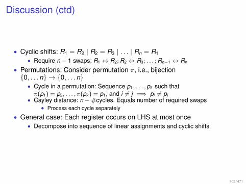
Discussion (ctd)

• Cyclic shifts: R1 = R2 | R2 = R3 | . . . | Rn = R1

• Require n − 1 swaps: R1 ↔ R2; R2 ↔ R3; . . . ; Rn−1 ↔ Rn

• Permutations: Consider permutation π, i.e., bijection{0, . . .n} → {0, . . .n}• Cycle in a permutation: Sequence p1, . . . , pk such thatπ(p1) = p2, . . . , π(pk ) = p1, and i 6= j =⇒ pi 6= pj

• Cayley distance: n −#cycles. Equals number of required swaps• Process each cycle separately

• General case: Each register occurs on LHS at most once• Decompose into sequence of linear assignments and cyclic shifts

402 / 471

Interprocedural Register Allocation

• For every local variable, there is an entry in the stack frame• Save locals to stack before call, restore after call• Sometimes, there is hardware support for this• Otherwise, we have to insert load and stores. We may ...

• Save only registers which may actually be overwritten• Save only registers which are live after the call• May restore into different registers =⇒ reduction of live ranges

403 / 471

Table of Contents

1 Introduction



4 Alias Analysis







404 / 471

Motivation

• Modern processors do not execute instructions one after the other• Each instruction passes multiple phases

• which are independent, and thus can be done in parallel for multipleinstructions

• Pipelining• Hardware for executing instructions is duplicated (superscalar

processors)• Independent instructions can be executed simultaneously• Usually combined with pipelining

• Who decides what instructions to parallelize• The compiler. =⇒ VLIW - architectures

• E.g., IA64, on Itanium processors• The processor (e.g. x86)

• Compiler should arrange instructions accordingly

405 / 471

Pipelining

• Execute instruction in multiple phases• e.g., fetch, decode, execute, write• Which are handled by different parts of the processor

• Idea: Keep all parts busy by having multiple instructions in the pipeline• Problem: Instructions may depend on each other

• e.g., R2 = 0; R = R+1; R = R+R• execute phase of second instruction cannot start, until write-phase of first

instruction completed

• Pipeline stall.• But compiler could have re-arranged instructions

• R = R+1; R2= 0; R = R+R

406 / 471

Superscalar architectures

• Fetch > 1 instruction per cycle.• Execute them in parallel if independent• Processor checks independence

• Out-of-order execution: Processor may re-order instructions

• Or compiler checks independence (VLIW)

407 / 471

Exam

• You may bring in two handwritten A4 sheets• We will not ask you to write OCaml programs

408 / 471

Last Lecture

• Register allocation• by coloring interference graph• by going to SSA-form

• Instruction level parallelism• Pipelining, superscalar architectures

409 / 471

Observation

• These architectures are profitable if there are enough independentinstructions available

• Here:1 Re-arrange independent instructions (in basic blocks)2 Increase size of basic blocks, to increase potential for parallelizing

410 / 471

Data dependence graph

• Consider basic block a1; . . . ; an

• Instructions ai and aj , i < j , are dependent, iffread-write ai reads register written by ajwrite-read ai writes register read by ajwrite-write ai and aj both write same register

• Dependence graph: Directed graph with• V := {a1, . . . , an}• (ai , aj ) ∈ E iff ai and aj are dependent

• Instructions in basic block can be reordered• As long as ordering respects dependence graph

411 / 471

Example

1: x=x+12: y=M[A]3: t=z4: z=M[A+x]5: t=y+z

Possible re-ordering:

2: y=M[A]1: x=x+13: t=z4: z=M[A+x]5: t=y+z

1: x=x+1 2: y=M[A] 3: t=z

4: z=M[A+x]

5: t=y+z

wrrw

wr

wr ww

412 / 471

Instruction Scheduling

• Goal: Find topological ordering that stalls pipeline as few as possible• Problems: Data dependencies, limited processor resources (e.g., only single

floating-point unit)• In general: NP-hard problem

• Common heuristics: List scheduling• While scheduling, keep track of used processor resources

• Requires (more or less precise) model of processor architecture

• Assign priorities to source nodes in graph• Schedule node with highest priority first• Heuristics for priorities

• If required resources are blocked: Lower priority• If dependencies not yet available: Lower priority• If node creates many new sources: Rise priority• If node lies on critical path: Rise priority

413 / 471

Example: Live-range splitting

• Live-range splitting helps to decrease dependencies• No re-ordering possible

1: x=r2: y=x+13: x=s4: z=x+1

• Can be re-ordered

1: x1=r2: y=x1+13: x2=s4: z=x2+1

• Re-ordering

1: x1=r3: x2=s2: y=x1+14: z=x2+1

• Some processors do that dynamically=⇒ Register renaming

414 / 471

Loop unrolling• Consider the example

short M [...];for (i=0;i<n;++i) {

M[i] = 0}

• On 32 bit architecture: Writing 16 bit words• Expensive!

• Consider unrolled loop (unroll factor 2)

short M [...];for (i=0;i+1<n;) {

M[i] = 0i=i+1M[i] = 0i=i+1

}if (i<n) {M[i]=0; i=i+1} // For odd n

short M [...];for (i=0;i+1<n;i=i+2) {(int)M[i] = 0

}if (i<n) {M[i]=0; i=i+1} // For odd n

• Loop body can now easily be optimized, e.g., by peephole optimization

415 / 471

Discussion

• Loop unrolling creates bigger basic blocks• Which open more opportunities for parallelization• Quick demo with gcc -O2 -funroll-loops

416 / 471

Loop fusion

• Fuse together two successive loops• With the same iteration scheme• That are not data-dependent

• for (...) {c1}; for (...) {c2} 7→ for (...) {c1;c2}

• In general:• i th iteration of c1 must not read data, that is written in < i th iteration of c2

• i th iteration of c2 must not read data, that is written in > i th iteration of c1

• Heuristics• Data written to disjoint places

• E.g., different, statically allocated arrays

• More sophisticated analyses, e.g., based on integer linear programming

417 / 471

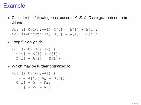
Example

• Consider the following loop, assume A,B,C,D are guaranteed to bedifferent

for (i=0;i<n;++i) C[i] = A[i] + B[i];for (i=0;i<n;++i) D[i] = A[i] - B[i];

• Loop fusion yields

for (i=0;i<n;++i) {C[i] = A[i] + B[i];D[i] = A[i] - B[i]}

• Which may be further optimized to

for (i=0;i<n;++i) {R1 = A[i]; R2 = B[i];C[i] = R1 + R2;D[i] = R1 - R2}

418 / 471

Warning

• The opposite direction, loop fission, splits one loop into two• May be profitable for large loops

• Smaller loops may fit into cache entirely• Accessed memory more local, better cache behavior

419 / 471

Table of Contents

1 Introduction



4 Alias Analysis







420 / 471

Motivation

• Aligning of data• Cache-aware data access• Reduction of allocation/deallocation cost

421 / 471

Alignment of data

• Processor usually loads 32/64 bit words from memory• But only from address which is multiple of 4/8• Read from odd addresses needs to be split• Expensive

• So compilers can align data in memory accordingly• Data on stack (parameters, local variables)• Code (labels, functions, loop-heads)• Layout of structures

• At the cost of wasting more memory

422 / 471

Cache-aware data access

• Load instruction loads whole cache-line• Subsequent loads within the same cache-line much faster• Re-arrange memory accesses accordingly• Important case: Multi-dimensional arrays

• Iteration should iterate according to memory layout

423 / 471

Example

• Array A[N][M]• Assume layout: &(A[i,j]) = i + j*N

• for (i=0;i<N;++i) for (j=0;j<M;++j) x=x+A[i,j]• Memory accesses:

A + 0 + 0N,A + 0 + 1N,A + 0 + 2N, ...,A + 1 + 0N,A + 1 + 1N, ...• Bad locality, when arriving at A + 1 + 0N, cache-line loaded on A + 0 + 0N

probably already overwritten• Better: for (j=0;j<M;++j) for (i=0;i<N;++i) x=x+A[i,j]

• Memory accesses: A + 0 + 0N,A + 1 + 0N, ...,A + 0 + 1N,A + 1 + 1N, ...• Good locality, A + 1 + 0N probably already in cache

424 / 471

Loop interchange

• Swap inner and outer loop• If they iterate over multi-dimensional array ...• ... in wrong order• And loop iterations are sufficiently independent

• Iteration for index i, j , must only depend on iterations ≤ i,≤ j• Illustration on board!

• The required dependency analysis is automatable• To some extend for arrays• Not so much for more complex structures

425 / 471

Organizing data-structures block-wise

• Warning: No automation in general• Example: Stack-data structure with push, pop

• Possible implementation: Linked list• Disadvantage: Data items distributed over memory• Bad cache behavior• And extra memory for link-pointers

• Alternative: Array-List• Keep list in array, store index of last element• If array overflows: Double the size of the array• If array less than quarter-full: Halve the size of the array• This adds amortized constant extra cost• But makes cache-locality much better

426 / 471

Moving heap-allocated blocks to the stack

• Idea: Allocate block of memory on stack, instead of heap• If pointers to this block cannot escape the current stack frame• Important for languages like Java, where almost everything is allocated on

heap

427 / 471

Abstract example

int do_computation(...) {AuxData aux = new AuxData ()...return ...

}

• If no pointer to aux is returned or stored in global memory ...• ... aux can be allocated on method’s stack-frame

428 / 471

Example

• Recall our simple pointer-language. Ret is global variable.

1: x=new()2: y=new()

x[A] = yz=x[A]Ret = z

• Allocation at 1 may not escape• Thus we may do the allocation on the stack

429 / 471

In general

• Memory block may escape, which is• Assigned to global variable• Reachable from global variable

• Forward may analysis. Same as pointer-analysis• Identify memory blocks with allocation sites• Analyze where variables/blocks may point to• If global variable/unknown memory block may point to block: Possible

escape

430 / 471

Applying the optimization, heuristics

• Only makes sense for small blocks• That are allocated only once

• e.g., not inside loop

431 / 471

Handling procedures more precisely

• Require interprocedural points-to analysis• Expensive• We do not always know whole program

• E.g. Java loads classes at runtime

• In worst case: Assume everything visible to called procedure may escape• Which is consistent with parameter passing by global variables and previous

analysis

432 / 471

Wrap-Up

• Several optimizations that exploit hardware utilization• A meaningful ordering

1 Restructuring of procedures/loops for better cache-behaviour• Loop interchange, fission• Tail-recursion/inlining, stack-allocation

2 Basic-block optimizations, to exploit instruction-level parallelism• Live-range splitting• Instruction scheduling• Loop unrolling, fusion

3 Then register allocation4 And finally peephole optimization + instruction selection

433 / 471

Table of Contents

1 Introduction



4 Alias Analysis







434 / 471

Last Lecture

• Optimizations to re-arrange memory access wrt. cache• Loop interchange• Lists vs. array-list

• Wrap-Up: Optimizations targeted towards features of hardware• Started with functional languages

435 / 471

Functional language

• We consider simple functional language

prg ::= let rec f1 = e1 | ... | f_n = e_n in ee ::= b | c | x | f_i | op | e e | fn x. e

| let x=e in e| match e with p1 => e1 | ... | p_n => e_n

p ::= b | c x1 ... xn

• where• b is primitive constant• c is constructor• x is variable• fi is recursive function• op is primitive operation

436 / 471

Table of Contents

1 Introduction



4 Alias Analysis






10 Optimization of Functional ProgramsSemanticsSimple OptimizationsSpecializationDeforestation

437 / 471

Semantics• Values b, c v1 . . . vn, fn x . e (Convention: v denotes values)• Goal of semantics: Evaluate main expression to value• Done by the following rules

[rec]let rec f_i = e_i

fi → ei

[op]−

op b1 . . . bn → [[op]](b1, . . . , bn)

[app1]e1 → e′1

e1 e2 → e′1 e2[app2]

e2 → e′2v1 e2 → v1 e′2

[β−red ]−

(fn x . e) v → e[x 7→ v ]

[match1]e→ e′

match e with . . .→ match e′ with . . .

[match2]−

match v with . . .→ eiσ(∗)

[app−op]ek → e′k

op v1 . . . vk−1 ek . . . en → op v1 . . . vk−1 e′k . . . en

• where let x = e1 in e2 is syntax for (fn x . e2) e1

• (*): pi =>ei is the first pattern with piσ = v438 / 471

Semantics

• Eager evaluation• Arguments are evaluated before function is called

• No types: Evaluation of badly-typed program just gets stuck• Example: match 5 with True => ... | False => ...

439 / 471

Exampleletrec fac = fn x. match x with

0 => 1| x => x * fac (x-1)

in fac 2

fac 2

(fn x. ...) 2

match 2 with ...

(*) 2 (fac (2-1))

(*) 2 ((fn x. ...) (2-1))

(*) 2 ((fn x. ...) 1)

(*) 2 (match 1 with ...)

(*) 2 ((*) 1 (fac (1-1)))

(*) 2 ((*) 1 ((fn x. ...) (1-1)))

(*) 2 ((*) 1 ((fn x. ...) 0))

(*) 2 ((*) 1 (match 0 with ...))

(*) 2 ((*) 1 1)

(*) 2 1

2

440 / 471

Lazy evaluation

• Evaluate arguments only when needed, as far as needed• I.e., on match or built-in function call

[rec]let rec f_i = e_i

fi → ei[op]

−op b1 . . . bn → [[op]](b1, . . . , bn)

[app1]e1 → e′1

e1 e2 → e′1 e2[β−red ]

−(fn x . e1) e2 → e1[x 7→ e2]

[match1]e→ e′

match e with . . .→ match e′ with . . .

[match2]−

match c e1 . . . ek with . . .→ eiσ(∗)

[match3]−

match b with . . .→ eiσ(∗)

[app−op]ek → e′k

op v1 . . . vk−1 ek . . . en → op v1 . . . vk−1 e′k . . . en

• Note: Only simple patterns allowed in match

441 / 471

Example (lazy)letrec fac = fn x. match x with

0 => 1| x => x * fac (x-1)

in (fac 2)

(fac 2)

((fn x. ...) 2)

(match 2 with ...)

((*) 2 (fac (2-1)))

((*) 2 ((fn x. ...) (2-1)))

((*) 2 (match (2-1) with ...))

((*) 2 (match 1 with ...))

and so on ...

442 / 471

Eager vs. Lazy

• Eager: Argument evaluated before function call• Lazy: Function call before argument

• Argument of match only until constructor is at top• Weak head normal form

• Arguments of primitive operator: Completely

443 / 471

Optimization Plan

• Optimize on functional level• Translate to imperative language/IR• Use optimizations for imperative code• Now: Optimizations on functional level

444 / 471

Table of Contents

1 Introduction



4 Alias Analysis







445 / 471

Simple optimizations

• Idea: Move some evaluation from run-time to compile-time• Function-application to let

(fn x. e1) e2 --> let x=e2 in e1

• Matches, where part of the pattern is already known

match c e1 ... e_n with ... c x1 ... xn => e> let x1=e1; ...; xn =e_n in e

• Let-reduction

let x=e1 in e --> e[x 7→e1]

446 / 471

Substitution

• Beware of name-capture

let x = 1 inlet f = fn y. x+y inlet x = 4 in

f x

• Consider reduction of f = . . ..

• α-conversion: (Consistent) renaming of (bound) variables does notchange meaning of program

• Convention: Substitution uses α-conversion to avoid name-capture• Here: Convert let x=4 in f x to let x1=4 in f x1

447 / 471

Termination issues

• Let-reduction may change semantics

let rec f = fn x. 1 + f x inlet _ = f 0 in

42

• This program does not terminate• But, applying let-reduction, we get

let rec f = fn x. 1 + f x in42

• which returns 42

• For eager evaluation, non-terminating programs may be transformed toterminating ones

• For lazy evaluation, semantics is preserved

448 / 471

Side-effects

• Languages like SML/OCaml/F# have side-effects• Side-effecting expressions must not be let-reduced

let _ = print "Hello"in ()

449 / 471

Application of let-reduction

• May make program less efficient• Re-computing values instead of storing them in variable

let x=expensive-op in x+x

• May blow up program code exponentiallylet x = x+x in let x = x+x in ... in x

• Heuristics for application: reduce let x1=e1in e• if e1 is a variable (or constant)• if x1 does not occur in e• if x1 occurs exactly once in e

450 / 471

More transformations

• Valid for programs (fragments) with no side-effects

(let x=e in e1) e2 --> let x=e in e1 e2// Renaming x to avoid name capture

let x1=e1 in let x2=e2 in e--> let x2=e2 in let x1=e1 in e

// If x1 not free in e2// Renaming x2 to avoid name capture

let x1 = (let x2=e2 in e1) in e--> let x2=e2 in let x1=e1 in e

// Renaming x2 to avoid name capture

• May open potential for other optimizations

451 / 471

Inlining

• Consider program let f=fn x. e1in e

• Inside e, replace f e2 by let x=e2in e1

• Goal: Save overhead for function call• Warning: May blow up the code

452 / 471

Examplelet fmax = fn f. fn x. fn y.if x>y then f x else f y in

let max = fmax (fn x. x) in...

let fmax = fn f. fn x. fn y.if x>y then f x else f y in

let max = (let f = (fn x. x) infn x. fn y. if x>y then f x else f y) in...

(inlined fmax)


let max = (let f = (fn x. x) infn x. fn y. if x>y then let x=x in x else let x=y in x) in...

(inlined f)


let max = (fn x. fn y. if x>y then x else y) in...

(Let-reduction for single-var expressions and unused variables)

453 / 471

Note• Inlining can be seen as special case of let-reduction• However: Does not change termination behavior or side-effects

• Only inlining terms of form fn x. e, which are not evaluated, unlessapplied to an argument

• In untyped languages (e.g., LISP), the inlining optimization may notterminate

let w = fn f. fn y. f (y f y) inlet fix = fn f. w f w

let w = fn f. fn y. f (y f y) inlet fix = fn f. let f=f in let y=w in f (y f y)

(Inlined w)

let w = fn f. fn y. f (y f y) inlet fix = fn f. f (w f w)

((Safe) let-reduction (copy variables))

let w = fn f. fn y. f (y f y) inlet fix = fn f. f (f (f (... f (w f w))))

( ... )• In typed languages like OCaml or Haskell, however, we have

• Inlining always terminates454 / 471

Table of Contents

1 Introduction



4 Alias Analysis







455 / 471

Specialization of recursive functions• Function to square all elements of a list

• Note: Dropping the restriction that let-rec occurs outermost• Requires many function calls to f• Idea: Replace map f by new function mapf• Specialization of map for argument f

let rec map = fn f. fn l.match l with

[] => []| x#l => f x # map f l

inlet f = fn x. x*x inlet sqrl = map f in ...

let rec map = fn f. fn l.match l with[] => []

| x#l => f x # map f linlet f = fn x. x*x inlet rec mapf = fn l.match l with[] => []

| x#l => f x # mapf linlet sqrl = mapf in ...

(Specialization)

let rec map = fn f. fn l.match l with[] => []

| x#l => f x # map f linlet f = fn x. x*x inlet rec mapf = fn l.match l with[] => []

| x#l => x*x # mapf linlet sqrl = mapf in ...

(Inlining)

456 / 471

Function folding

• When specializing function f a to fa,• we may replace f a by fa in definition of fa• Beware of name-captures!

• If recursive function calls alter the specialized argument:• Potential for new specializations may be created• Infinitely often ...• let rec f = fn g. fn l. ... f (fn x. g (g x)) ...

• Safe and simple heuristics:• Only specialize functions of the form

let rec f = fn x. e

such that recursive occurrences of f in e have the form f x

457 / 471

Table of Contents

1 Introduction



4 Alias Analysis







458 / 471

Deforestation

459 / 471

Deforestation

• Idea: Often, lists are used as intermediate data structures• Standard list functions

let rec map = fn f. fn l. match l with[] => []

| x#xs => f x # map f xs

let rec filter = fn P. fn l. match l with[] => []

| x#xs => if P x then x#filter P xs else filter P xs

let rec foldl = fn f. fn a. fn l. match l with[] => []

| x#xs => foldl f (f a x) xs

460 / 471

Deforestation

• Examples of derived functions

let sum = foldl (+) 0

let length = sum o map (fn x. 1)

let der = fn l.let n = length l inlet mean = sum l / n inlet s2 = (

sumo map (fn x. x*x)o map (fn x. x-mean)) l

ins2 / n

461 / 471

Idea

• Avoid intermediate list structures• E.g., we could define

length = foldl (fn a. fn _. a+1) 0

• In general, we can define rules for combinations of the basic list functionslike fold, map, filter, ...

map f o map g = map (f o g)foldl f a o map g = foldl (fn a. f a o g) afilter P o filter Q = filter (fn x. P x & Q x)...

• We may also need versions of these rules in first-order form, e.g.map f (map g l) = ...

462 / 471

Examplelet der = fn l.let n = length l inlet mean = sum l / n inlet s2 = (

sumo map (fn x. x*x)o map (fn x. x-mean)) l

ins2 / n

let der = fn l.let n = length l inlet mean = sum l / length l inlet s2 = (

foldl (+) 0o map (fn x. x*x)o map (fn x. x-mean)) l

ins2 / n

Let-optimization/ inlining

let der = fn l.let n = length l inlet mean = sum l / length l inlet s2 = (

foldl (+) 0o map ((fn x. x*x) o (fn x. x-mean))) l

ins2 / n

map-map rule

let der = fn l.let n = length l inlet mean = sum l / length l inlet s2 = foldl (

fn a. (+) a o (fn x. x*x) o (fn x. x-mean)) 0 l

ins2 / n

fold-map rule

let der = fn l.let n = length l inlet mean = sum l / length l inlet s2 = foldl (

fn a. fn x. let x=x-mean in let x=x*x in a+x) 0 l

ins2 / n

function-application, unfolding of o, let-optimization.

463 / 471

Discussion

• Beware of side-effects!• Need rules for many combinations of functions.

• Does not scale• Only works for built-in functions

• Could try to automatically recognize user-defined functions• Can be extended to algebraic datatypes in general

• They all have standard map and fold functions

464 / 471

Reducing the number of required rules

• Try to find standard representation• foldr seems to be a good candidate:

foldr f a [] = afoldr f a (x#xs) = f x (foldr f a xs)

• We can represent map, filter , sum, ...• But no list-reversal, as foldl can

• Problem: How to compose two foldr-calls?• foldr f1 a1 (foldr f2 a2 l) = ???

465 / 471

Composition of foldr

• Idea: Abstract over constructors

map f l = foldr (fn l. fn x. f x#l) [] l

map’ f l = fn c. fn n.foldr (fn l. fn x. c (f x) l) n l

build g = g (#) []map f l = build (map’ f l)

• Have

foldr f a (build g) = g f a

• If abstraction over list inside g done properly• I.e., g actually produces list using its arguments

466 / 471

Example

map f (map g l)

= build (map’ f (build (map’ g l)))

= build (fn c. fn n.foldr (fn l. fn x. c (f x) l) n (build (map’ g l)))

= build (fn c. fn n. map’ g l (fn l. fn x. c (f x) l) n)

467 / 471

Intuition

• Functions may consume lists (foldr ), produce lists (build), or both• Applying a chain of functions: (build foldr) (build foldr) . . . (build foldr)

• Can be re-bracketed to build (foldr build) . . . (foldr build) foldr• And the inner pairs cancel out, leaving a single build foldr

468 / 471

Discussion

• Single rule for deforestation: foldr f a (build g) = g f a• Only correct if g is abstracted over list correctly• Consider, e.g., foldr f a (build (fn _. fn _. [True]))

• Which is, in general, not the same as (fn _. fn _. [True]) f a

• If language is parametric, can be enforced via type:• If g has type ∀β.(A→ β → β)→ β → β• It can only produce its result of type β by using its arguments• Which is exactly the required abstraction over the list constructors

469 / 471

Wrap-up

• Transformations for functional programs• Let-optimization• Inlining• Specialization• Deforestation• ...

• Aim at reducing complexity before translation to IR• On (imperative) IR, all former optimizations of this lecture can be done

• Important one: Tail-call optimization• There are no loops in functional languages

470 / 471

That’s it!Questions?

471 / 471

Program Optimization - TUM

Documents

Transcript of Program Optimization - TUM