Profinite Groups and Infinite Galois...

U.U.D.M. Project Report 2019:52

Examensarbete i matematik, 15 hpHandledare: Martin HerschendExaminator: Veronica Crispin QuinonezNovember 2019

Department of MathematicsUppsala University

Profinite Groups and Infinite Galois Extensions

Jonatan Lindell

Abstract. In the 1930’s Wolfgang Krull extended the fundamental theorem of Galois theory toinfinite Galois extension via introducing a topology on the Galois group. This gave a correspondencebetween closed subgroups and intermediate fields. The aim of this thesis is to show that every Galoisgroup is a profinite group, use this to prove the theorem of Krull and lastly as well show that everyprofinite group can be realised as a Galois group of a Galois extension.

Contents

1. Introduction 22. Conventions 23. Groups and Rings 33.1. Group Theory 33.2. Ring Theory 64. Field Theory 104.1. Algebraic Extensions 124.2. Splitting Fields and Normal Extensions 144.3. Separable Extension 164.4. Galois Extensions 185. Topological Spaces and Topological Groups 215.1. Basic Topology 215.2. Topological Groups 266. Inverse Limits 286.1. Inverse limits of sets 286.2. Profinite Spaces 317. Profinite Groups and Galois Extensions 357.1. Profinite Groups 357.2. Profinite Groups as Galois groups 388. Further Generalization 43Acknowledgments 43References 43

1

1. Introduction

The modern version of Galois theory as the study of field extension and automorphism groups wasfirst developed by Emil Artin from earlier work going back to several authors, including EveristeGalois [5]. One of the most important theorems, if not the most important theorem, of Galoistheory is the fundamental theorem of finite Galois extension which gives a bijective correspondencebetween intermediate field extensions of a finite field extension and the subgroups of the Galoisgroup of the extension. This is important as it allows us to use group-theoretical tools to studycertain field extensions.

During the 1930’s Krull extended the fundamental theorem of Galois theory to infinite Galoisextension using topology. The aim of this thesis is to give a proof of the theorem that Krull provedand to give a connection between profinite groups and Galois groups. To do this we will give anintroduction of Galois theory, starting from group theory and ring theory. We will then give acondensed introduction to topology as well as an introduction to topological groups. Followed bythis we will give an introduction to profinite groups and give a characterisation of profinite groups.Lastly we will connect profinite groups to Galois groups and prove Krull’s theorem.

We will assume basic knowledge of set theory. Both the introduction to topology and Galois theorywe will be quite terse, so therefore it will be helpful to have some familiarity with basic topologyand basic algebra, though not formally needed.

2. Conventions

Here we will quickly repeat some definitions from set theory to make sure that we are all on thesame page. For this section we will basically follow [3].

We will denote that A is a subset of or equal to B by A ⊆ B. If A is a subset of B that is notequal to B we say that A then is a proper subset and denote this by A $ B.

Definition 2.0.1. Let A and B be two sets, then we define a map f between A and B to bea subset of A × B such that for all a ∈ A there exists one pair (a, b) such that (a, b) ∈ f . Wedenote (a, b) ∈ f by f(a) = b. If f is a map from A to B we write f : A → B. We will use map,function and morphism interchangeably. If f : A→ B and g : B → C are maps, then we define thecomposition of f with g as the set

{(a, d) ∈ A× C | There exists (a, b) ∈ f and (c, d) ∈ g such that b = c}. (1)

We denote the composition g ◦ f .

We will use “a 7→ b” to denote that a function maps a to b.

Definition 2.0.2. Let A and B be sets and let f : A→ B be a map. Then

(a) f is surjective if for all b ∈ B there exists a a ∈ A such that f(a) = b;(b) f is injective if for all a1, a2 ∈ A such that f(a1) = f(a2), we have that a1 = a2.(c) f is bijective if it is surjective and injective.

Definition 2.0.3. Let A be a set and let f : A → A be a map. Then we say that f is anendomorphism. If f is also bijective we say that f is an automorphism.

Proposition 2.0.4. Let A and B be sets and let f : A → B be a bijective map. Then g ={(b, a) | (a, b) ∈ f} is a map and g ◦ f = idA and f ◦ g = idB.

Proof. It follows from that f is surjective that for every b ∈ B there exists a pair (b, a) ∈ g. It alsofollows from that f is injective that there exists only one such pair for each b ∈ B. Thus g is amap. That g ◦ f = idA and f ◦ g = idB follows from the definition of composition of maps. �

2

Definition 2.0.5. Let A and B be sets and let f : A→ B be a bijective map. We then define theinverse of f to be the map define in the above proposition. We denote the inverse of f by f−1.

Definition 2.0.6. Let A,B,C,D be sets and let f : A → C and let g : B → D. Then we definethe product map of f, g from A × B → C ×D to be the map defined by (a, b) 7→ (f(a), g(b)). Wedenote this map f × g.

Definition 2.0.7. Let A and B be two sets, we say that A and B are isomorphic if there existsmaps f : A→ B and g : B → A such that g ◦ f = idA and f ◦ g = idB. We denote this A ∼= B.

Proposition 2.0.8. Let A and B be sets. Then A ∼= B if and only if there exists a bijective mapf : A→ B.

Proof. Assume that A ∼= B. Then by definition there exists f : A → B, g : B → A such thatg ◦ f = idA and f ◦ g = idB. We aim to show that f is bijective. Firstly f is surjective as if b ∈ B,then for a = g(b), we get that f(a) = b as f ◦ g = idB. Secondly f is injective as if f(a1) = f(a2)then a1 = g(f(a1)) = g(f(a2)) = a2 as g ◦ f = idA. Thus f is bijective. Conversely assume f isbijective. Then the result follows by Proposition 2.0.4. �

Definition 2.0.9. A commutative diagram is a collection of objects and morphisms such thatfor any path (morphism seen as directed edges) between any two objects the compositions of themorphisms in the respective paths are equal.

This is much easier understood by seeing an example.

Example 2.0.10. Let A = N, B = Z, C = R and D = C. Let f be function defined by x 7→ x2,g the function defined by x 7→ x3, h the function defined by x 7→ x6 and j the function defined byx 7→ x. We say that the following diagram commutes as g ◦ f = j ◦ h.

A B

C D

f

h g

j

3. Groups and Rings

Here we will give a short introduction to basic group and ring theory. The proofs and expositionwill follow Chapters I, II and III in [4].

3.1. Group Theory.

Definition 3.1.1. A group is a set G together with a map · : G × G → G, called multiplication,such that the following condition are fulfilled.

(a) There exists a element e ∈ G such that a · e = e · a = a for all a ∈ G. We call such anelement the identity element. This element is unique.

(b) For all a, b, c ∈ G, we have that (a · b) · c = a · (b · c).(c) For all a ∈ G there exists a element a−1 ∈ G such that a · a−1 = a−1 · a = e. We call a−1

the inverse element of a.

We often denote a group by only its underlying set. We will also often write ab instead of a · b.

One geometric way to think about a group is that is describe the symmetries of an object. Forexample if we take the set of all reflective and rotational symmetries of triangle we get a group.We define the operation on this group as composition of these operation.

Example 3.1.2. Here are some examples of groups.

(a) The set Z with the operation · defined as addition.3

(b) The set Q \ {0} with the operation · defined as usual multiplication.(c) The set R \ {0} with the operation defined likewise.(d) The set of n× n invertible matrices, with operation being matrix multiplication.

Here are two examples of things that are not groups.

(a) The set Z with the operation being defined as usual multiplication.(b) The set of n× n matrices with the operation being defined as matrix multiplication.

Definition 3.1.3. Let (G, ·) be a group. If for all a, b ∈ G, a · b = b · a holds, then we say that thegroup is abelian (after Niels Henrik Abel) and we often denote · by + and the identity by 0 instead.

Definition 3.1.4. A subgroup of a group G is a non-empty subset H ⊆ G such that H is closedunder multiplication and inverses. We denote this by H ≤ G.

We say that a subgroup is trivial if it only consists of the identity element.

The following proposition is often easier and quicker to use than the definition.

Proposition 3.1.5. Let G be a group, and H ⊆ G be a subset of G. Then H is a subgroup of Gif and only if for all a, b ∈ H it holds that ab−1 ∈ H and H 6= ∅.

Proof. Assume that H is a subgroup of G. Then H is by definition closed under inverse and thusfor all a ∈ H, a−1 ∈ H. Therefore we have that, as H is closed under products, that for alla, b ∈ H, ab−1 ∈ H. By definition H is also non-empty. Conversely assume that for all a, b ∈ Hthat ab−1 ∈ H. Then we have that e ∈ H as aa−1 = e and by assumption aa−1 ∈ H. Therefore wealso have that a−1 ∈ H for all a ∈ H by assumption as a−1 = ea−1. Therefore it remains to showthat H is closed under products, but this follows as ab = a(b−1)−1 for all a, b ∈ H. �

The following definition we will need for two important concepts, normal subgroups and quotientgroups.

Definition 3.1.6. Let G be a group and let H be a subgroup. We then define

(a) a left-coset of H to be the set aH = {ah | h ∈ H} for some a ∈ G;(b) a right-coset of H to be the set Ha = {ha | h ∈ H} for some a ∈ G.

Now we can define what we mean by a normal subgroup.

Definition 3.1.7. Let G be a group and let N ≤ G be a subgroup. We then say that N is normalif for all g ∈ G, gN = Ng. We denote this by N EG.

Note that if a group is abelian then every subgroup is normal. We also have the following propositionregarding normal subgroups.

Proposition 3.1.8. Let G be a group and let H be a subgroup G. Then H is normal if and onlyif gNg−1 ⊆ N for all g ∈ G.

Proof. Note that gNg−1 ⊆ N for all g ∈ G is equivalent to that g−1Ng ⊆ N for all g ∈ G. We firstprove the if direction. Assume that gNg−1 ⊆ N for all g ∈ G. Then let gn ∈ gN , then gng−1 = n′

for some n′ ∈ N , thus gn = n′g and therefore gn ∈ Ng. Conversely let ng ∈ Ng then g−1ng = n′

for some n′ ∈ N , therefore ng = gn′ and thus ng ∈ gN . Therefore gN = Ng for all g ∈ G. We nowprove the only if direction. Assume that gN = Ng for all g ∈ G. Then let gng−1 ∈ gNg−1. Thengn = n′g for some n′ ∈ N and thus gng−1 = n′ ∈ N . Therefore gNg−1 ⊆ N for all g ∈ G. �

Next we will define what a morphism of groups is.

Definition 3.1.9. Let G and H be two groups. A group morphism f : G → H is map such thatfor all a, b ∈ G, f(ab) = f(a)f(b).

4

The following properties of group morphisms are easily verified.

Lemma 3.1.10. Let f : G→ H be a group morphism. Then the following is true.

(a) f(a−1) = f(a)−1 for all a ∈ G.(b) f(eG) = eH .

Next we define two important subsets connected to morphisms.

Definition 3.1.11. Let G and H be groups, and let f : G→ H be a group morphism.

(a) The kernel of a morphism is the set of elements that gets map to the identity element. Wedenote this by ker(f) = {g ∈ G | f(g) = eH}.

(b) The image of a morphism is the set of elements that lie in the set f(G). We denote this byLet im(f) = {h ∈ H | There exists a g ∈ G such that f(g) = h}.

Note that a morphism is surjective if and only if the image of the morphism is the whole group.Note also that a morphism is injective if and only if the kernel is trivial.

Proposition 3.1.12. Let G and H be groups, and let f : G→ H be a group morphism. Then thefollowing is true.

(a) ker(f) is a normal subgroup of G.(b) im(f) is subgroup of H.

Proof. We begin by proving (a). We start by showing that ker(f) is a subgroup. By Proposi-tion 3.1.5 we only need to show that ker(f) is nonempty and that for all a, b ∈ ker(f) we havethat ab−1 ∈ ker(f). That the kernel is nonempty follows by Lemma 3.1.10 as f(eG) = eH . Nowlet a, b ∈ ker(f). Then, by Lemma 3.1.10, we have that f(ab−1) = f(a)f(b)−1 = e · e−1 = e.Therefore, as a, b ∈ ker(f) were arbitrary, it follows that ker(F ) is a subgroup of G. To show thatker(f) is normal we will use Proposition 3.1.8. Let g ∈ G and n ∈ ker(f) be arbitrary. Thenf(gng−1) = f(g)f(n)f(g)−1 = f(g)ef(g)−1 = e and thus it follows that gng−1 ∈ ker(f) for allg ∈ G and all n ∈ ker(f). Therefore ker(f) is normal.

We now prove (b). That im(f) is nonempty follows directly from the definition. Let a, b ∈ im(f),then there exists a′, b′ ∈ G such that a = f(a′) and b = f(b′). Note that ab−1 ∈ im(f) as a′b′−1 ∈ Gand f(a′b′−1) = f(a′)f(b′)−1 = ab−1. Therefore im(f) is a subgroup of H. �

Next we define a concept that we will need briefly for the Galois theory in later sections.

Definition 3.1.13. Let G be a group and let H1 and H2 be subgroups of G. We then say that H1

is conjugate to H2 if there exists an element g ∈ G such that gH1g−1 = H2.

Note that normal subgroups only have one conjugate, itself.

Proposition 3.1.14. Let G be a group and let H be a subgroup of G. Then the number of rightcosets of H are equal to the number of left cosets of H.

For a proof see Proposition 3.12 in Chapter I, section 3 of [4].

Thus by knowing this, we know that it doesn’t matter if we choose the left or right cosets for thefollowing definition.

Definition 3.1.15. Let G be a group and let H be a subgroup. The index of H is the number ofleft cosets.

We can now finally define what a quotient group is.5

Proposition 3.1.16. Let G be an group and let N be a normal subgroup. Then we define G/N tobe the set of all left-cosets G/N = {aN | a ∈ G} and endow it with the operation defined as follows,aN · bN = abN . Then G/N is a group.

For a proof of this see Proposition 4.7 in Chapter I, section 4 of [4].

Definition 3.1.17. We call G/N , defined as above, the quotient group of G by N .

One way to think about quotient group is that we take away everything that we don’t want, so tospeak, i.e. that lying in N . Note that xN = yN if and only if y−1x ∈ N . Therefore we could alsohave define the quotient group via the equivalence relation x ∼ y if y−1x ∈ N .

The following two theorems were first proved by Emmy Noether in 1927 for modules [9]. Especiallythe first theorem here we will be very important and often used for the rest of thesis.

Theorem 3.1.18 (First isomorphism theorem). Let f : G → H be a group morphism, then there

exists a isomorphism f : G/ker(f) → im(f) defined by aker(f) 7→ f(a). In particular if f issurjective then G/ker(f) ∼= H.

Proof. We first prove that f is well defined. Note that aker(f) = bker(f) is equivalent to thatab−1 ∈ ker(f). Let aker(f) = a′ker(f), then f(aa′−1) = eH which implies that f(a) = f(a′). Hence

f is well defined. Next we prove that f is group morphism. Let aker(f), bker(f) ∈ G/ker(f),

then f((ab)ker(f)) = f(ab) = f(a)f(b) = f(aker(f)) + f(bker(f)). By definition we have that f issurjective, thus we only need to prove injectivity. Assume that f(a) = f(b) then this implies thatf(ab−1) = eH . Therefore ab−1 ∈ ker(f) and thus aker(f) = bker(f). �

Next we prove the second isomorphism, which says that in some cases we can treat quotients asusual division.

Theorem 3.1.19 (Third isomophism theorem). Let G be a group and let H be a normal sub-group, and let N be a normal subgroup of H. Then H/N is a normal subgroup of G/N and(G/N)/(H/N) ∼= (G/H).

Proof. Let aN ∈ H/N then gNaNg−1N = gag−1N ∈ H/N . Therefore by Proposition 3.1.8H/N is a normal subgroup of G/N . Define f : G/N 7→ G/H by aN 7→ aH. To see that itwell defined note that if ab−1 ∈ N then ab−1 ∈ H as N ⊆ H. Next we show that f is a groupmorphism. We have that f((ab)N) = (ab)H = abH = f(a)f(b). Thus f is a group morphism.Note that ker(f) = {aN ∈ G/N | a ∈ H} = H/N and that f is surjective. Therefore we get byTheorem 3.1.18 that (G/N)/(H/N) ∼= (G/H). �

3.2. Ring Theory. Now we will give some basic results in ring theory.

Definition 3.2.1. A ring is a three tuple (R,+, ·) of a set R, an operation + : R×R→ R and aoperation · : R × R → R such that (R,+) is abelian group, with the identity element denoted by0, and such that the following condition are fulfilled.

(a) For all a, b, c ∈ R, we have that (a · b) · c = a · (b · c).(b) There exists a element 1 ∈ R, such that 1 · a = a · 1 = a for all a ∈ R.(c) For all a, b, c ∈ R, we have that a · (b+ c) = (a · b) + (a · c).(d) For all a, b, c ∈ R, we have that (b+ c) · a = (b · a) + (c · a).

We will, as with groups, often denote a ring only by its underlying set. We will also often write abinstead of a · b. We call the operation + addition and the operation · multiplication. The identityof element of + and · is called the additive, respectively multiplicative, identity element. We saythat a ring is commutative if ab = ba for all a, b ∈ R.

6

Example 3.2.2. Here we give some examples of rings.

(a) (Z,+, ·) with addition and multiplication defined as usual is a ring.(b) (Q,+, ·) with addition and multiplication defined likewise.(c) The set of all n× n matrices with addition and multiplication defined as usual is a ring.

We will from now on assume that all rings are commutative. We next define what a subring is.

Definition 3.2.3. Let (R,+, ·) be a ring. A subring (A,+, ·) of R is subset A ⊆ R such thatfollowing conditions are fulfilled.

(a) (A,+) is subgroup of (R,+).(b) (A,+, ·) is closed under multiplication and it contains the multiplicative identity element 1.

Example 3.2.4. For example (Q,+, ·) is a subring of (R,+, ·).Now we define the corresponding notation of normal subgroups but for rings.

Definition 3.2.5. Let R be a ring and let I ⊆ R be a subset. We call I an ideal if (I,+) is asubgroup of (R,+) and rI ⊆ I for all r ∈ R. We say that an ideal is proper if I $ R.

We define what a ring morphism is.

Definition 3.2.6. Let R,S be rings and let ϕ : R → S. We then say that ϕ : R → S is a ringmorphism the following condition are fulfilled.

(a) The map ϕ : (R,+)→ (S,+) is a group morphism.(b) For all r1, r2 ∈ R, ϕ(r1r2) = ϕ(r1)ϕ(r2).(c) ϕ(1R) = 1S .

Likewise as we define the kernel and image of a group morphism we can define the kernel and imageof a ring morphism.

Definition 3.2.7. Let R and S be rings and let ϕ : R→ S be a ring morphism. Then we define

(a) the kernel of ϕ to be the set ker(ϕ) = {r ∈ R | ϕ(r) = 0};(b) the image of ϕ to be the set im(ϕ) = {s ∈ S | There exists a r ∈ R such that ϕ(r) = s}.

Proposition 3.2.8. Let R and S be a rings and let ϕ : R→ S be a ring morphism. Then

(a) ker(ϕ) is an ideal of R;(b) im(ϕ) is a subring of S.

Proof. We first prove that the kernel ofR is an ideal. We know by Proposition 3.1.12 that (ker(ϕ),+)is a subgroup of (R,+). Thus we only need to show that rker(ϕ) ⊆ ker(ϕ) for all r ∈ R. Note thatϕ(ra) = ϕ(r) · 0 = 0 for all a ∈ ker(ϕ). Thus we have that rker(ϕ) ⊆ ker(ϕ).

Now we prove that im(ϕ) is a subring of S. We know by Proposition 3.1.12 that (im(ϕ),+) isa subgroup of (S,+). Thus it remains to show that 1 ∈ im(ϕ) and that if a, b ∈ im(ϕ) thenab ∈ im(ϕ). Firstly note that 1 ∈ im(ϕ) as by definition ϕ(1) = 1. Next let a, b ∈ im(ϕ) then thereexists a′, b′ ∈ R such that ϕ(a′) = a and ϕ(b′) = b. Thus ϕ(a′b′) = ab and therefore ab ∈ im(ϕ). �

Like we can quotient groups by normal subgroups, we can quotient rings by ideals.

Proposition 3.2.9. Let R be a ring and let I be an ideal. Let S be the quotient group (S,+) givenby R/I, seeing I as a normal subgroup, with multiplication defined as (a+ I)(b+ I) = ab+ I. ThenS is a ring.

For a proof of this see Proposition 3.3 in section 3 of Chapter III in [4].

Definition 3.2.10. Let R be a ring and let I be an ideal. We define the quotient ring of R by Ito be the ring S in the above proposition. We denote this R/I.

7

Now we will prove the first isomorphism theorem for rings. Like the one for groups this will bevery important for the rest of the thesis.

Theorem 3.2.11 (First Isomorphism Theorem). Let ϕ : R → S be a ring morphism. ThenR/ker(ϕ) ∼= im(ϕ), with the isomorphism given by aker(ϕ) 7→ ϕ(a).

Proof. We know by Theorem 3.1.18 that we have isomorphism f of the underlying additive groupsgiven by a+ ker(ϕ) 7→ ϕ(a). Thus if we can show that this is also a ring morphism we will be done.

Let a+ker(ϕ), b+ker(ϕ) ∈ R/ker(ϕ), then f((a+ker(ϕ))(b+ker(ϕ))) = f((ab)+ker(ϕ)) = ϕ(ab) =

ϕ(a)ϕ(b) = f(a+ ker(ϕ))f(b+ ker(ϕ)). Thus it remains to show that f(1 + ker(ϕ)) = 1 but this is

true as f(1 + ker(ϕ)) = ϕ(1) = 1. �

In the rest of this subsection we will describe several important properties and types of rings. Webegin with one of the most basic (in the sense that it pops up often).

Definition 3.2.12. Let R 6= {0} be a ring. Then we say that R is an integral domain if R for alla, b ∈ R we have that ab = 0 implies that either a = 0 or b = 0.

Another way of phrasing this definition is that there aren’t two non-zero element such that theproduct of these two elements are zero.

Example 3.2.13. We now give one example of a field that is not an integral domain and of onethat is.

(a) Let Z/12Z be the ring of all integers modulo 12. Then 6 · 2 = 0 mod 12 but 6 6= 0 and2 6= 0. Therefore Z/12Z is not an integral domain.

(b) Let Z be the ring of all integers, then this is integral domain.

Next we define elements that have multiplicative inverses.

Definition 3.2.14. Let R be a ring and let a ∈ R. We then say that a is a unit if there exists anelement r ∈ R such that ar = ra = 1. We denote the set of all units of ring by R∗.

Next we generalise the notation of divisors, prime and irreducible from the natural numbers.

Definition 3.2.15. Let R be a integral domain. We say that an element a ∈ R divides an elementb if b = ac for some c ∈ R. We denote this a|b. We say that a non-unit p is

(a) prime if p|ab implies that p|a or p|b for all a, b ∈ R;(b) irreducible if p = ab implies that a or b is a unit for all a, b ∈ R.

Now we can generalise the notation of prime elements to ideals.

Definition 3.2.16. Let R be a ring and let I ⊂ R be a proper ideal. We say that I is a primeideal if for all ab ∈ I implies that either a ∈ I or b ∈ I.

Definition 3.2.17. Let R be a ring and let I ⊆ R be an proper ideal. We say that I is a maximalideal if there exists no proper ideal J such that I $ J .

We will now define two important types of rings, principal ideal domains and unique factorisationdomains. Both of these properties generalise in some sense the properties of Z. Principal idealdomains are rings where every ideal is generated by one element, and unique factorisation domainsare rings where every element can be factorised uniquely into irreducible elements.

Definition 3.2.18. Let R be a ring and let I be an ideal of R. We say that I is a principal idealif I = Ra = {ra | r ∈ R} for some fixed a ∈ R. We then say that I is generated by a and denotethis as I = (a).

8

Definition 3.2.19. Let R be an integral domain. We say that R is a principal ideal domain,shortened PID, if every ideal of R is principal.

The following is an important property of PIDs.

Proposition 3.2.20. Let R be a PID. Then every non-trivial prime ideal is a maximal ideal.


Definition 3.2.21. Let R be an integral domain. We say that R is a unique factorization domain,shortened UFD, if every non-zero element can be written uniquely on the form upk00 p

k11 ...p

knn , where

u is a unit and p0, ..., pn are irreducible elements of R and ki ∈ N. More precisely by uniquely wemean that if upko0 ...p

knn = vql00 ...q

lmm then n = m and up to reordering Rpi = Rqi for all i.

The following proposition says that in a UFD there is no difference between being irreducible andbeing prime.

Proposition 3.2.22. Let R be a UFD and let a ∈ R. Then a is irreducible if and only if a isprime.


The following theorem allows us to in one direction connect the two concepts.

Theorem 3.2.23. Every PID is a UFD.

For a proof of this see Theorem 8.4 in section 8 of Chapter III in [4].

If we draw a diagram of the different types of rings we get the following.

Rings (not necessarily commutative) ⊇ Commutative Rings ⊇ Integral Domains ⊇ UFDs ⊇ PIDs

Next we generalise the notation of polynomials by letting the coefficients lie in an arbitrary ring,instead of just being real numbers as when one often first encounters them.

Proposition 3.2.24. Let R be a ring. Let S be sets consisting of elements of the form r0 + r1x+r2x

2 + ... + rnxn where r0, ..., rn ∈ R, n ∈ N and x is an indeterminant. Define addition between

the elements the following way

(r0 + ...+ rnxn) + (s0 + ...+ smx

m) = q0 + ...+ qkxk

where k = max{n,m}, qi = ri + si and where we define ri = 0 if i > n and si = 0 if i > m. Definemultiplication between the elements the following way

(r0 + ...+ rnxn)(s0 + ...+ smx

m) = q0 + ...+ qkxk

where k = n + m, qi = r0si + r1si−1 + ... + ri−1s1 + ris0 and where we define ri = 0 if i > n andsi = 0 if i > m. Then this is a ring.


Definition 3.2.25. Let R be a ring. We define the polynomial ring of R to be the ring define inthe above proposition. We denote this ring R[x].

Proposition 3.2.26. Let ϕ : R → S be a ring morphism, then this induces a ring morphismfϕ : R[x]→ S[x] defined by fϕ(anx

n + ...+ a0) = ϕ(an)xn + ...+ϕ(a0). If q is a polynomial in R[x]then we denote the image of q under fϕ by qϕ.

9

Proof. Let a = a0 + ...+ anxn, b = b0 + ...+ bmx

m ∈ R[x] be given. Then

fϕ(a+ b) = fϕ(q0 + ...+ qkxk) = ϕ(q0) + ...+ ϕ(qk)x

k = fϕ(a) + fϕ(b)

where k = max{n,m}, qi = ai + bi and where ai = 0 if i > n and bi = 0 if i > m. Likewise

fϕ(ab) = fϕ(s0 + ...+ skxk) = ϕ(s0) + ...+ ϕ(sk)x

k = fϕ(a)fϕ(b)

where k = n + m, si = a0bi + a1bi−1 + ... + ai−1b1 + aib0 and where ai = 0 if i > n and bi = 0 ifi > m. Note that fϕ(1) = ϕ(1) = 1. Thus fϕ is ring morphism. �

Next we have the following important theorem.

Theorem 3.2.27. Let R be a ring. If R is a UFD then R[x] is a UFD.

For a proof of this see Theorem 10.4 in section 10 of Chapter III in [4].

4. Field Theory

Here we will study field extensions, mainly to get to Galois extensions. The proofs and expositionof this section will mainly follow Chapter IV and V in [4].

Definition 4.0.1. A field is a ring (F,+, ·) such that F ∗ = F \ {0}.

We usually (that is the rest of the thesis) denote a field only by its underlying set. Intuitively onecan think of a field as a set where we can add, subtract, multiply and divide numbers as usual.Note that the definition assures that a field has at least two elements.

Example 4.0.2. The following examples are fields

(a) The set of rational numbers Q, where multiplication is normal multiplication and additionis normal addition.

(b) The set of real numbers R, defined likewise.(c) The set of complex numbers C, defined likewise.(d) Z/pZ, where p is a prime number.

Definition 4.0.3. The characteristic of a field F is the smallest n ∈ Z+ such that n · 1 = 0. If nosuch n exists we say that the characteristic is zero.

Now we have the following proposition regarding rings that we will need for later propositions.

Proposition 4.0.4. Let R be a ring and let I ⊆ R be an ideal.

(a) I is a prime ideal if and only if R/I is an integral domain.(b) I is a maximal ideal if and only if R/I is a field.

Proof. We begin by proving (a). Assume that I is a prime ideal. Let a+ I, b+ I ∈ R/I and assumethat ab+ I = 0 + I. This is equivalent to that ab ∈ I. But this implies that either a ∈ I or b ∈ I asI is prime. Assume without loss of generality that a ∈ I. Then we get that a+ I = 0 + I. As a andb were arbitrary it follows that R/I is a integral domain. Conversely assume that R/I is a integraldomain. Let ab ∈ I, then ab+ I = 0 + I in R/I and thus as R/I is an integral either a+ I = 0 + Ior b + I = 0. But this implies that either a or b lie in I. Therefore, as a and b were arbitrary itfollows that I is a prime ideal.

Next we prove (b). Assume that I is a maximal ideal. Then we need to show that every elementis unit except zero. Let a ∈ R/I be a non-zero elemnt. Then Ra+ I is an ideal of R containing I.This implies that Ra + I = R as I is maximal. Therefore there exists r ∈ R and i ∈ I such thatra+ i = 1. This implies that (ra+ i) + I = (ra) + I = (r + I)(a+ I) = 1 + I and therefore a+ Iis unit. Thus we get that R/I is a field. Conversely assume that R/I is a field and that J is an

10

ideal such that I ( J ⊆ R. Then there exists a ∈ J \ I and therefore a + I is a non-zero elementin R/I. This implies that there exists b + I ∈ R/I such that (ab) + I = 1 + I. This is equivalentto that (1 − ab) ∈ I which implies that (1 − ab) ∈ J . Note also that ab ∈ J as J is an ideal of R.Therefore we get that ab+ (1− ab) = 1 ∈ J and thus J = R. Therefore I is maximal. �

Note that every field is a PID as the only ideals of a field F are (0) and F . We also have thefollowing proposition.

Proposition 4.0.5. Let F be a field, then F [x] is PID.

For a proof of this see Proposition 5.12 in section 5 of Chapter III in [4].The following proposition will be often used later.

Proposition 4.0.6. Let F be a field and let f ∈ F [x] be a irreducible polynomial. Then (f) is amaximal ideal, and thus F [x]/(f) is a field.

Proof. Firstly by Proposition 4.0.5 we know that F [x] is a PID. We also have by Theorem 3.2.23that F [x] is a UFD. Therefore we can conclude by Proposition 3.2.22 (f) is also a non-trivial primeideal. Lastly it follows by Proposition 3.2.20 that (f) is a maximal ideal. Then F [x]/(f) is a fieldby Proposition 4.0.4. �

We will now define what a field morphism is.

Definition 4.0.7. Let F and E be fields, a field morphism is a mapϕ : F −→ E such that ϕ(1) = 1, ϕ(ab) = ϕ(a)ϕ(b) and ϕ(a+ b) = ϕ(a) + ϕ(b).

Note that this is the same as the definition of a ring morphism except that the domain and codomainof the map are now fields.

Proposition 4.0.8. Every field morphism is injective.

Proof. Let ϕ : F −→ E be a field morphism. Then since F is a field, the only ideals of F are (0) orF . As ker(ϕ) is an ideal we have that ker(ϕ) = (0) as otherwise ϕ(1) = 0, hence ϕ is injective. �

Now we come to one of the most basic definitions of the thesis, namely field extensions.

Definition 4.0.9. A field extension of a field F is an field E such that F ⊆ E. We denote thisE/F . The dimension of the field extension is the dimension of E as an vector spaces over F . Wedenote this by [E : F ]. We say that a field extension E/F is finite if [E : F ] <∞Example 4.0.10. The following are examples of field extensions

(a) For any field F , F itself is an extension of F and [F : F ] = 1.(b) C is an extension of R and [C : R] = 2.(c) The dimension of an extension can also be infinite e.g R is an infinite extension of Q.

Proposition 4.0.11. Let E/F be a field extension and let L be an intermediate field extension,F ⊆ L ⊆ E. Then [E : F ] = [E : L][L : F ].

Proof. Let (αi)i∈I be a basis for L/F and let (βj)j∈J be a basis for E/L. Then every element inE can be written as a linear combination of βj ’s, where in turn each term can be written as alinear combination of αi’s. More concretely if a ∈ E then we know that a =

∑j∈J ajβj , aj ∈ L

and βj ∈ E. In turn aj =∑

i∈I bijαi, bij ∈ F and α ∈ L. Thus a =∑

(i,j)∈I×J bij(αiβj).

Thus we want to show that (αiβj)(i,j)∈I×J forms a basis for E over F . That it spans E wehave already established, thus we only need to show that it is linear independent. Assume that∑

(i,j)∈I×J aij(αiβj) = 0 then this is equivalent to that∑

j∈J(∑

i∈I aijαi)βj = 0, which implies that∑i∈I aijαi = 0, as (β)j∈J is linearly independent, which in turn implies that aij = 0 as (αi)i∈I

is linearly independent. Thus (αiβj)(i,j)∈I×J is a basis for E over F . Therefore we have that[E : F ] = |I × J | = |I||J | = [E : L][L : F ]. �

11

Definition 4.0.12. Let E/F and E/L be a field extensions. A F -morphism ϕ : E → L is a fieldmorphism such that f|F = idF .

We will now define two ways of constructing new fields that will be used often.

Proposition 4.0.13. Let E be a field extension of F , and let S ⊆ E be a subset of E. ThenF [S], generated by F ∪ S, is the ring of linear combinations of finite powers of elements of S withcoefficients in F . The field F (S), generated by F ∪ S, is the field of ab−1 ∈ E, b 6= 0, wherea, b ∈ F [S].

For a proof of this see Proposition 1.9 in section 1 of Chapter IV in [4].

We can likewise define this for polynomials.

Proposition 4.0.14. Let F be a field. Then we define the set

F (x) = {pq| p, q ∈ F [x] and q 6= 0}/∼

where the equivalence relation is given by pq ∼

p′

q′ if pq′ = p′q. Then this is field where addition is

defined by pq + p′

q′ = pq′+qp′

qq′ and where multiplication is defined by pq ·

p′

q′ = pp′

qq′ .

For a proof of this see Proposition 4.10 in section 4 of Chapter III of [4].

Definition 4.0.15. Let E be a field extension F . We say that E is finitely generated whenE = F (α0, ..., αk), for some αi ∈ E. If E = F (α), for some α ∈ E, we say that E is a simpleextension of F .

Note that every finite extension is finitely generated. One important meta-method is that when wehave a finite extension F (α1, ..., αn)/F we can build a tower of simple extension

F = F0 ⊆ F1 ⊆ F2 ⊆ ... ⊆ Fn−1 ⊆ Fn = F (α1, ..., αn)

where we define Fi = Fi−1(αi). The following proposition is important as it allows us to connectthe degree of a simple extension to degree of a polynomial.

Proposition 4.0.16. Let F be a field and let E be a field extension of F . Let α ∈ E.

(a) If f(α) 6= 0 for all f ∈ F [x] and then F (α) ∼= F (x) for an indeterminant x.(b) If f(α) = 0 for some f ∈ F [x] and then there exists a unique irreducible monic polynomial

g ∈ F [x] such that g(α) = 0. Then F (α) ∼= F [x]/(g), the degree of the extension is the

degree of g, and 1, α, α2, ..., αdeg(g)−1 forms a basis for F (α) over F . We also have that forany polynomial h such that h(α) = 0 it is the case that g|h.

We denote the unique irreducible monic polynomial of an algebraic element α ∈ E determined by(b) by irr(α : F ). For a proof of this see Proposition 2.2 in section 2 of Chapter IV in [4].

4.1. Algebraic Extensions. Now we generalise the concept of algebraic numbers to arbritraryfield extensions.

Definition 4.1.1. Let F be a field and let E be an extension of F . We say that α ∈ E is algebraicover F if there exists a polynomial f ∈ F [x] such that f(α) = 0. An extension E of F is algebraicif each element in E is algebraic over F .

Proposition 4.1.2. Every finite extension is algebraic.12

Proof. Let E/F be a finite extension and assume that [E : F ] = n. Let α ∈ E \ F be an arbitraryelement. Consider {1, α, α2, ..., αn}. Since this set contains n + 1 vectors it follows that the setmust be linearly dependent and thus a0 + a1α+ ...+ anα

n = 0 for some a0, ..., an ∈ F . Now definef(x) = a0 + ... + anx

n, then f(α) = 0 and thus α is algebraic over F . As α was arbitrary it nowfollows that E/F is an algebraic extension. �

We now give some properties of algebraic extensions.

Proposition 4.1.3. Assume that E/F is an algebraic extension, and let L be an intermediatefield F ⊆ L ⊆ E. Then E/L and L/F are algebraic extensions if and only if E/F is an algebraicextension.

Proof. First assume that E/F is algebraic and let α ∈ E. Then there exists f ∈ F [x] such thatf(α) = 0 and as F [x] ⊆ L[x] we have that α is algebraic over L. Let β ∈ L be given, then thereexists g ∈ F [x] such that g(β) = 0 as L ⊆ E. Thus β is algebraic over F .

Now conversely assume that E/L and L/F are algebraic extensions. Let α ∈ E be given. Thenthere exists a irreducible polynomial f = a0 + ... + anx

n ∈ L[x] such that f(α) = 0. Then wehave that α is algebraic over K = F (a0, ..., an). Therefore K(α)/K is an algebraic extension and[K(α) : F ] = [K(α) : K][K : F ] by Proposition 4.0.11. By Proposition 4.0.16 we have that[K(α) : K] = deg(f). Thus [K(α) : F ] is finite. Hence by Proposition 4.1.2 we get that K(α)/F isalgebraic and therefore α is algebraic over F . Thus, as α was arbitrary, E/F is algebraic. �

Proposition 4.1.4. Let F and E be fields and let α be algebraic over F . Let f = irr(α : F ). Ifψ : F (α)→ E is a field morphism and ϕ is a restriction of ψ to F , then ψ(α) is a root of fϕ in E.Conversely, for every field morphism ϕ : F → E and every root β of fϕ in E, there exists a uniquefield morphism ψ : F (α)→ E that extends ϕ and sends α to β.

F F (α)

E

⊆

ϕ ψ


Definition 4.1.5. Let F be a field, we then say that F is algebraically closed if it fulfills any ofthese following equivalent properties.

(a) The only algebraic extension of F is F itself.(b) All irreducible polynomials are of degree 1.(c) Every nonconstant polynomial in F [x] has a root in F .

We now prove that these three properties actually are equivalent

Proof. We will start by proving that (a) implies (b). Let p ∈ F [x] be an irreducible polynomial.Then F [x]/(p) is an algebraic extension of F , since it is finite. By (a) the degree of the extensionmust be one and hence by Proposition 4.0.16 deg(p) = 1.

We will now prove that (b) implies (c). Let p ∈ F [x] be a polynomial of degree 1. Then p(x) = ax+bfor some a, b ∈ F where a 6= 0. Then (−b)a−1 ∈ F is a root of p. Therefore all polynomials of degree1 has a root in F and since they are the only irreducible polynomials by (b), every non-constantpolynomial has a root in F as F [x] is a UFD.

Finally we prove that (c) implies (a). Assume there exists an algebraic extension E/F other thanF . Then α ∈ E is algebraic over F . Let f = irr(α : F ), then by (c) f must have a root r ∈ F . As f

13

is irreducible and monic it must be the case that f = x− r. Therefore, as f(α) = 0, we have thatα = r ∈ F and thus the only algebraic extension of F is F itself. �

The proof of the following theorem relies on Zorn’s lemma. For proofs of the following theoremsof this subsection see Theorem 4.2, Lemma 4.3 and Theorem 4.4 in section 4 of Chapter IV in [4,p. 166-168].

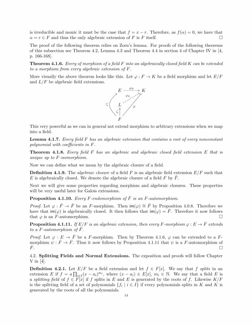
Theorem 4.1.6. Every of morphism of a field F into an algebraically closed field K can be extendedto a morphism from every algebraic extension of F .

More visually the above theorem looks like this. Let ϕ : F → K be a field morphism and let E/Fand L/F be algebraic field extensions.

E K

L

F

ϕE

ϕL

ϕ

⊆

⊆

This very powerful as we can in general not extend morphism to arbitrary extensions when we mapinto a field.

Lemma 4.1.7. Every field F has an algebraic extension that contains a root of every nonconstantpolynomial with coefficients in F .

Theorem 4.1.8. Every field F has an algebraic and algebraic closed field extension E that isunique up to F -isomorphism.

Now we can define what we mean by the algebraic closure of a field.

Definition 4.1.9. The algebraic closure of a field F is an algebraic field extension E/F such thatE is algebraically closed. We denote the algebraic closure of a field F by F .

Next we will give some properties regarding morphism and algebraic closures. These propertieswill be very useful later for Galois extensions.

Proposition 4.1.10. Every F -endomorphism of F is an F -automorphism.

Proof. Let ϕ : F → F be an F -morphism. Then im(ϕ) ∼= F by Proposition 4.0.8. Therefore wehave that im(ϕ) is algebraically closed. It then follows that im(ϕ) = F . Therefore it now followsthat ϕ is an F -automorphism. �

Proposition 4.1.11. If E/F is an algebraic extension, then every F -morphism ϕ : E → F extendsto a F -automorphism of F .

Proof. Let ϕ : E → F be a F -morphism. Then by Theorem 4.1.6, ϕ can be extended to a F -morphism ψ : F → F . Thus it now follows by Proposition 4.1.11 that ψ is a F -automorphism ofF . �

4.2. Splitting Fields and Normal Extensions. The exposition and proofs will follow ChapterV in [4].

Definition 4.2.1. Let E/F be a field extension and let f ∈ F [x]. We say that f splits in anextension E if f = a

∏i∈I(x − ai)mi , where (x − ai) ∈ E[x], mi ∈ N. We say that a field E is

a splitting field of f ∈ F [x] if f splits in E and E is generated by the roots of f . Likewise K/Fis the splitting field of a set of polynomials {fi | i ∈ I} if every polynomials splits in K and K isgenerated by the roots of all the polynomials.

14

Lemma 4.2.2. If E and L are splitting fields of a set S ⊆ F [x] over F , and L ⊆ F , then for everyF -morphism ϕ : E → F , ϕ(E) = L.

For a proof of this see Lemma 1.1 in section 1 of Chapter V in [4].

Proposition 4.2.3. Let F be a field. Then every set S ⊆ F [x] has a splitting field, and moreoverall the splitting fields of S are F -isomorphic.

For a proof of this see Proposition 1.2 in section 1 of Chapter V in [4].

Thus we now can speak of the splitting field of a set of polynomials (up to isomorphism). We nowdefine what a normal extension is.

Definition 4.2.4. A field extension E/F is normal if it is the splitting field of a set polynomialsS ⊆ F [x].

We now give some properties of normal extensions.

Proposition 4.2.5. Let E/F be a field extension, then the following are equivalent.

(a) E is the splitting field of a set of polynomials.(b) For every F -morphism ϕ : E → F , satisfies that ϕ(E) = E.(c) For every F -morphism ϕ : E → F , satisfies that ϕ(E) ⊆ E.(d) For every F -automorphism ϕ : F → F , satisfies that ϕ(E) = E.(e) For every F -automorphism ϕ : F → F , satisfies that ϕ(E) ⊆ E.(f) Every irreducible polynomial f ∈ F [x] with a root in E, splits in E

Proof. (a) ⇒ (b):This follows by Lemma 4.2.2.

(b) ⇒ (c): This follows as if ϕ(E) = E then by definition ϕ(E) ⊆ E.

(b) ⇒ (d): Let ϕ : F → F be an F -automorphism, then ϕ|E : E → F is a F -morphism and by (b)ϕ(E) = ϕ|E(E) = E.

(c) ⇒ (e): Let ϕ : F → F be an F -automorphism, then ϕ|E : E → F is a F -morphism and by (b)ϕ(E) = ϕ|E(E) ⊆ E.

(d) ⇒ (e): This follows as if ϕ(E) = E then per definition ϕ(E) ⊆ E.

(e) ⇒ (f): Let f ∈ F [x] be an arbitrary irreducible polynomial with a root α ∈ E. For every rootβ ∈ F of f there exists, by Proposition 4.1.4, a F -morphism ϕ : F (α) → F that sends α to β.By Proposition 4.1.11, ϕ extends to a F -automorphism σ : F → F . Thus, by (e), β = σ(α) ∈ E.Therefore E contains every root of f and thus f splits in E[x].

(f) ⇒ (a): Let S = {irr(α : F ) | α ∈ E}. Then every f ∈ S has a root in E and so therefore splitsin E. Moreover E is generated by the roots of these polynomials and thus it is the splitting fieldof S. �

Unfortunatley normality does not transfer as strongly to intermidiate field extension compared toalgebraic extensions.

Proposition 4.2.6. Let F ⊆ L ⊆ E be field extensions, and assume that E/F is normal. ThenE/L is normal.

15

Proof. By definition E/F is normal if E is the splitting fields of set of polynomials S ⊆ F [x]. AsS ⊆ F [x] ⊆ L[x] we have that E/L is normal. �

We now generalise the concept of conjugates from C to arbritrary fields.

Definition 4.2.7. Let F be a field and let a ∈ F . We then say that an element b ∈ F is a conjugateof a over F if b = ϕ(a) for some F -automorphism ϕ : F → F .

Definition 4.2.8. Let E/F be an algebraic extension and assume that E ⊆ F . We then say thata field L is a conjugate of E if it is the image of E under a F -automorphism of F .

Proposition 4.2.9. Let F be a field and let a ∈ F . Then the conjugates of a are the roots ofirr(a : F ) in F .

For a proof of this see Proposition 2.2 in section 2 in Chapter V in [4].

Proposition 4.2.10. Let E/F be a algebraic extension and assume that E ⊆ F . Then followingproperties are equivalent.

(a) E/F is a normal extensions;(b) For every element α ∈ E, E contains all the conjugates of α over F .(c) E has only itself as it conjugate.

Proof. This equivalence follows from Proposition 4.2.5. To see this more precisely, (b) follows from(f) in Proposition 4.2.5 by Proposition 4.2.9 as irr(α : F ) splits in E. Finally (c) follows by (d) inProposition 4.2.5. �

4.3. Separable Extension. We will now define what a separable extension is and give someproperties of said extensions.

Definition 4.3.1. A polynomial p ∈ F [x] is separable if p can be factored in F [x] as

p = (x− a0)(x− a1)...(x− an) (1)

where ai 6= aj if i 6= j. Let E be an extension of F , we then say that α ∈ E is separable if it isalgebraic over F and irr(α : F ) is separable. We say that an extension E/F is separable if everyelement of E is separable over F .

Alot of field extension are separable as the following proposition shows.

Proposition 4.3.2. Let F be a field of characteristic zero and let E/F be an algebraic extension.Then E/F is separable.


Now we will define what the separability degree of an extension is.

Definition 4.3.3. The separability degree of an algebraic extension E/F is the number of F -morphism ϕ : E → F . We denote this [E : F ]S .

Proposition 4.3.4. Let F be a field and let α be algebraic over F . Then [F (α) : F ]S is the numberof distinct roots of irr(α : F ). Thus [F (α) : F ]S ≤ [F (α) : F ].

Proof. Let f = irr(α : F ) and let ϕ : F (α)→ F be a F -morphism. As f ∈ F [x] we have that fϕ = fand therefore we get that 0 = fϕ(ϕ(α)) = f(ϕ(α)). Thus for any ϕ : F (α)→ F , ϕ(α) is a root of f .Therefore we have that the number of F -automorphism ϕ : F (α)→ F are equal to distinct roots off as these maps are uniquely determined from where they send α. We have, by Proposition 4.0.16,that [F (α) : F ] = deg(f) and therefore we have that [F (α) : F ]S ≤ [F (α) : F ]. �

The following Corollary follows directly from the above proposition.16

Corollary 4.3.5. Let F be a field and let α be algebraic over F . Then [F (α) : F ]S = [F (α) : F ] ifand only if irr(α : F ) is separable.

Like with the dimension of an extension we can split up the separability degree.

Proposition 4.3.6. If E/F is an algebraic extension and L is an intermediate field, then [E :F ]S = [E : L]S [L : F ]S.


Proposition 4.3.7. Let E/F be a finite extension. Then the following condition are equivalent.

(a) E is separable over F .(b) E is generated by finitely many separable elements.(c) [E : F ]S = [E : F ].

Proof. (a) ⇒ (b):As E/F is finite extension, we know that E = F (α1, ..., αn) for some α1, ..., αn ∈ E. Thus, as by(a) every element in E is separable, the results follows as therefore especially α1, ..., αn are separable.

(b) ⇒ (c):By assumption E = F (α1, ..., αn) for some separable α0, ..., αn ∈ E. Define the following interme-diate fields, E0 = F , Ei = Ei−1(αi). Thus we have the following tower of fields F = E0 ⊆ E1 ⊆... ⊆ En−1 ⊆ En = E. Let fi = irr(αi : Ei−1) and let gi = irr(αi : F ). We now by assumption thatgi is separable and as F [x] ⊆ Ei−1[x] we must have that fi|gi. Therefore fi is separable. Thus weget by repeated use of Proposition 4.3.6, Proposition 4.0.11 and Proposition 4.3.5

[E : F ]S = [En : En−1]S ...[E1 : E0]S

= [En : En−1]...[E1 : E0]

= [E : F ]

Thus we have proved (c).(c) ⇒ (a): Let α ∈ E be arbitrary. Then we have by assumption and by Proposition 4.3.6 andProposition 4.0.11 that

[E : F (α)]S [F (α) : F ]S = [E : F ]S = [E : F ]

= [E : F (α)][F (α) : F ]

We also know that, by Proposition 4.3.4 [F (α) : F ]S ≤ [F (α) : F ]. We also have that [E : F (α)]S ≤[E : F (α)]. To see this note firstly that E/F is algebraic by Proposition 4.1.2 and thereforeE = F (β1, ..., βn). Define E0 = F (α) and Ei = Ei−1(βi). Then we have that [E : F (α)]s =[E : En−1]s...[E1 : F (α)]s which is less than or equal to [E : En−1]...[E1 : F (α)] = [E : F (α)] byPropositio 4.3.4. Therefore [E : F (α)]s ≤ [E : F (α)]. Thus as E/F is a finite extension it must bethe case that [E : F (α)]S = [E : F (α)] and that [F (α) : F ]S = [F (α) : F ]. Therefore we have thatα is separable by Proposition 4.3.4 and as α ∈ E was arbitrary E/F is a separable extension. �

We now give some properties of separable extensions.

Proposition 4.3.8. Let E/F be a separable extension and let L be an intermediate extension.Then E/L and L/F are separable extensions if and only if E/F is separable.

Proof. First assume that E/F is algebraic and let α ∈ E. Then α is separable over L as F [x] ⊆ L[x].Thus E/L is separable. Let β ∈ L be given then β is separable over F as β ∈ E as L ⊆ E.

Conversely assume that E/L and L/F are separable extensions. Let α ∈ E is separable over L andirr(α : L) = a0 + ...+ anx

n. Then K = F (a0, ..., an) is separable over F as L/F is separable. Also17

K(α)/K is also separable as α is separable over L. Define K0 = F and Ki = Ki−1(ai−1), then wehave the following tower of extensions

F = K0 ⊆ K1 ⊆ ... ⊆ Kn−1 ⊆ Kn = K ⊆ K(α).

Then we get by Proposition 4.3.6, Proposition 4.3.5 and Proposition 4.0.11 that

[K(α) : F ] = [K(α) : K][K : Kn−1]...[K1 : F ]

= [K(α) : K]S [K : Kn−1]S ...[K2 : K1][K1 : F ]S

= [K(α) : F ]S

Therefore by Proposition 4.3.7 we get that K(α)/F is separable. Thus especially α is separableover F . Therefore, as α was arbitrary, we get that E/F is separable. �

Proposition 4.3.9. Every finite separable extension is simple.


Proposition 4.3.10. If E/F is separable and irr(α : F ) has degree at most n for every α ∈ E,then E/F is simple and [E : F ] ≤ n.


4.4. Galois Extensions. We will now define what Galois extensions and Galois groups are. Wewill then connect subgroups and intermediate field extensions via the fundamental theorem ofGalois extensions. The proofs and exposition of this section will mostly follow section 3 of ChapterV in [4].

Definition 4.4.1. An algebraic extension E of a field F is called a Galois extension of F if it isseparable and normal.

This definition may not make it entirely intuitive why we study precisely these extensions. Thefollowing theorem gives a maybe more intuitive explanation why these extension are interesting.

Theorem 4.4.2. Let E/F be a algebraic extension. Then E/F is a Galois extension if and onlyif every F -automorphism of E is the identity on and only on F .

We will later show the backwards direction of the if and only if statement but for all whole proofsee [1]. Note that a Galois extension in [1] is called a normal extension.

Given a Galois extension E/F we can study the group of F -automorphism.

Proposition 4.4.3. Let E/F be a field extension, then the set of all F -automorphism forms agroup with composition as the group operation.

Proof. Let G denote the set of all F -automorphisms. First by definition composition of functionare associative. We also have an identity element given by the idE : E → E as by definition for anyσ ∈ G, we have that σ ◦ idE = idE ◦ σ = σ. Note that as every σ ∈ G is bijective we have inversegiven by σ−1 ∈ G. Therefore G forms a group. �

Definition 4.4.4. Let E/F be a Galois extension, then we define the Galois group to be the groupof F -automorphisms. We denote this group by Gal(E/F ) for a Galois extension E/F .

Proposition 4.4.5. If E/F is a finite Galois extension, then |Gal(E/F )| = [E : F ].

Proof. As E/F is normal it follows by Proposition 4.2.5, that every F -morphism of E into F sendsE onto E. Therefore, if we restricted such a map to E it is precisely an F -automorphism of E.Hence it follows that |Gal(E/F )| = [E : F ]S = [E : F ] as E is also separable over F . �

18

Definition 4.4.6. Let G be a group of automorphism of a field F . We then defined the fixed fieldof G to be {a ∈ F | σa = a for all σ ∈ G}. We denote this by FixF (G).

We need to prove that this is also indeed a field.

Proof. Firstly by definition every field automorphism must fix 1 so therefore 1 ∈ FixF (G). Leta, b ∈ FixF (G), then by the definition of a group morphism and Lemma 3.1.10 we have that

(a) σ(ab) = σ(a)σ(b) = ab for all σ ∈ G, hence ab ∈ FixF (G);(b) σ(a+ b) = σ(a) + σ(b) = a+ b for all σ ∈ G, hence a+ b ∈ FixF (G);(c) σ(a−1) = σ(a)−1 = a−1 for all σ ∈ G, hence a−1 ∈ FixF (G);(d) σ(−a) = −σ(a) = −a for all σ ∈ G, hence −a ∈ FixF (G).

Therefore FixF (G) forms a field. �

Proposition 4.4.7. If G is a finite group of automorphism of a field E then E is a finite Galoisextension of F = FixE(G) and Gal(E/F ) = G.

Proof. We will begin by showing that E is algebraic over F . Let α ∈ E be an arbitrary element.Then, as G is finite, Gα = {β ∈ E | σα = β for some σ ∈ G} = {α1, α2, ..., αn}, where n ≤ |G| andα1, ..., αn ∈ E are distinct elements. Note that we must have that one of the αi is equal to α asG is a group and therefore contains the identity automorphism. Without loss of generality we willassume that α1 = α. We now define the polynomial fα(X) = (α1−X)(α2−X)...(αn−X) ∈ E[X].Then fα(α) = 0 and fα is separable. Moreover, every σ ∈ G permutes α1, ..., αn and therefore(fα)σ = fα. Thus fα ∈ F [X]. It now follows that α is algebraic over F and as irr(α : F ) mustdivide fα, α is also separable. Thus E is an algebraic and separable extension of F as α wasarbitrary. We also see that E is a splitting field of the polynomials fα ∈ F [X] for all α ∈ E, henceit also normal over F . We therefore conclude that E/F is a Galois extension.

By Proposition 4.3.10 it follows that [E : F ] ≤ |G| as E/F is a finite extension. We also have byProposition 4.4.5 that |Gal(E/F )| = [E : F ] ≤ |G|. But every σ ∈ G is an F -automorphism of E,so G ⊆ Gal(E/F ). Therefore we conclude that Gal(E/F ) = G. �

Proposition 4.4.8. If E/F is a Galois extension, then the fixed field of Gal(E/F ) is precisely F .

Proof. Let G = Gal(E/F ) and let L = FixE(G). Then F ⊆ L. Let α ∈ L, now we want to show thatα ∈ F . There exists an algebraic closure of F such that E ⊆ F . Every F -morphism ϕ : F (α)→ Fextends to a F -automorphism of F . As E/F is also a normal extension, we can restrict ϕ to aF -automorphism ψ of E. Hence ϕ(α) = ψ(α) = α, as α ∈ L = FixE(G). By definition ϕ is theinclusion morphism of F (α) into F . Thus [F (α) : F ]S = 1. Therefore, since F (α) ⊆ E is separableover F , this implies that F (α) = F , by Proposition 4.3.4. Therefore we conclude that α ∈ F andthus that F = L. �

We can now finally prove the fundamental theorem of finite Galois extensions.

Theorem 4.4.9. Let E/F be a finite Galois extension and let G = Gal(E/F ). Let F(E/F ) ={L | L is a field and F ⊆ L ⊆ E} and let S(G) = {H | H ≤ G}. We then have a bijection betweenF(E/F ) and S(G) via the map

Φ : F(E/F )→ S(G)

L 7→ Gal(E/L)

and the map

Γ : S(G)→ F(E/F )

H 7→ FixE(H)19

Proof. To show this we need to show that Φ ◦ Γ = idS(G) and that Γ ◦ Φ = idF(E/F ). Let H bea subgroup of G and let FixE(G) = L. Then it follows by Proposition 4.4.7 that G = Gal(E/F )and thus it follows that Φ ◦ Γ = idS(G). Likewise let L be an intermediate field then it follows thatΓ(Φ(L)) = L by Proposition 4.4.8. �

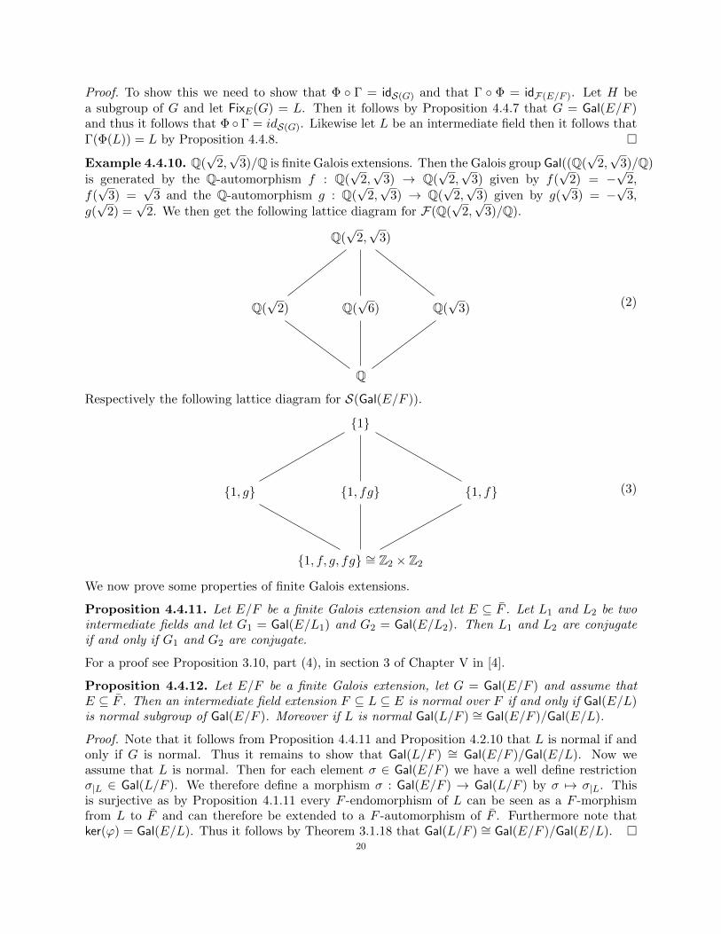
Example 4.4.10. Q(√

2,√

3)/Q is finite Galois extensions. Then the Galois group Gal((Q(√

2,√

3)/Q)is generated by the Q-automorphism f : Q(

√2,√

3) → Q(√

2,√

3) given by f(√

2) = −√

2,f(√

3) =√

3 and the Q-automorphism g : Q(√

2,√

3) → Q(√

2,√

3) given by g(√

3) = −√

3,g(√

2) =√

2. We then get the following lattice diagram for F(Q(√

2,√

3)/Q).

Q(√

2,√

3)

Q(√

2) Q(√

6) Q(√

3)

Q

(2)

Respectively the following lattice diagram for S(Gal(E/F )).

{1}

{1, g} {1, fg} {1, f}

{1, f, g, fg} ∼= Z2 × Z2

(3)

We now prove some properties of finite Galois extensions.

Proposition 4.4.11. Let E/F be a finite Galois extension and let E ⊆ F . Let L1 and L2 be twointermediate fields and let G1 = Gal(E/L1) and G2 = Gal(E/L2). Then L1 and L2 are conjugateif and only if G1 and G2 are conjugate.

For a proof see Proposition 3.10, part (4), in section 3 of Chapter V in [4].

Proposition 4.4.12. Let E/F be a finite Galois extension, let G = Gal(E/F ) and assume thatE ⊆ F . Then an intermediate field extension F ⊆ L ⊆ E is normal over F if and only if Gal(E/L)is normal subgroup of Gal(E/F ). Moreover if L is normal Gal(L/F ) ∼= Gal(E/F )/Gal(E/L).

Proof. Note that it follows from Proposition 4.4.11 and Proposition 4.2.10 that L is normal if andonly if G is normal. Thus it remains to show that Gal(L/F ) ∼= Gal(E/F )/Gal(E/L). Now weassume that L is normal. Then for each element σ ∈ Gal(E/F ) we have a well define restrictionσ|L ∈ Gal(L/F ). We therefore define a morphism σ : Gal(E/F ) → Gal(L/F ) by σ 7→ σ|L. Thisis surjective as by Proposition 4.1.11 every F -endomorphism of L can be seen as a F -morphismfrom L to F and can therefore be extended to a F -automorphism of F . Furthermore note thatker(ϕ) = Gal(E/L). Thus it follows by Theorem 3.1.18 that Gal(L/F ) ∼= Gal(E/F )/Gal(E/L). �

20

A question that one now might be wondering about is what happens if we take away the conditionof the Galois extension being finite in the main theorem. The problem we will see in later examplesis that we get too many subgroups, i.e subgroups of the Galois group that have the same fixedfield, thus losing our lovely bijection in the fundamental theorem. The strategy, as we will see inthe sections following, is to restrict which subgroups we take and then hopefully attain a bijectionin the infinite case. What Krull found out in the 1930’s is that the key is to introduce a topology.

5. Topological Spaces and Topological Groups

5.1. Basic Topology. Here will recall the basic definitions of topology as well as some results thatwe will need later. The proofs and exposition will basically follow [8].

A topology on a set allows us in an abstract way to “measure” how close two points are. Thus, aswe can “measure” closeness, we get a better grasp over infinite things, as we can say if somethingapproaches something else.

Definition 5.1.1. A topological space is a 2-tuple (X, T ), where X is set and T ⊆ P (X) is subsetof the power set of X, that fulfills the following conditions

(a) ∅ ∈ T and X ∈ T .(b) If (Ai)i∈I is a collection of sets, each in T , then

⋃i∈I Ai ∈ T .

(c) If (Ai)i∈I is a finite collection of sets, each in T , then⋂i∈I Ai ∈ T .

The sets in T are called open sets. We say that T defines a topology on X or that X is endowedwith the topology given by T . We say that a subset V ⊆ X is closed if X \V ∈ T . We denote thatan subset U is open in a topological space X by U ⊆op X and that U is closed by U ⊆cl X.

Note that we are allowed to take the union of any number of open sets, even a uncountable number,whilst we are only allowed to take the intersection of a finite number of open sets. We will often(almost always) denote a topological space only by its underlying set.

Example 5.1.2. We will now give a couple of examples and non-examples of topological spaces.

(a) Let X = {a, b, c} and let T = {X, {a, b}, {a}, {b}, ∅}. Then (X, T ) is a topological space.(b) Let X be as above and let T = {X, {a, b}, {a}, {c}, ∅}. Then (X, T ) is not a topological

space as for example {c} ∪ {a} 6∈ T .(c) Let X = N. Let T = {M ⊆ N | N \M is finite or M = ∅}. Then (X, T ) is a topological

space.

Definition 5.1.3. Let X be any set. Then we define the trivial topology as the topology given byT = {X, ∅} and the discrete topology on X as the topology given by letting every set be open.

Definition 5.1.4. Let (X, T ) be a topological space and let A ⊆ X. We then define the subsettopology on A as the topology given by T ′ = {A ∩ U | U ∈ T }.We now define what the structure preserving maps between topological space are.

Definition 5.1.5. Let X and Y be topological spaces. We say that a map f : X → Y is continuousif the preimage of every open set is open.

Example 5.1.6. We will now give a couple of examples of continuous maps.

(a) Let X = {a, b, c}, let T1 = {X, {a, b}, {a}, {b}, ∅} and T2 = {X, {b, c}, {b}, {c}, ∅}. Let f =idX and let g be the function defined by a 7→ b, b 7→ c and c 7→ a. Then f : (X, T1)→ (X, T1)is continuous but f : (X, T1)→ (X, T2) is not continuous. Likewise g : (X, T1)→ (X, T2) iscontinuous but g : (X, T1)→ (X, T1) is not continuous.

(b) Let X be any set endowed with the discrete topology and let Y be any topological space.Then any function f : X → Y is continuous.

21

(c) Let X and Y be any topological spaces. Fix a y0 ∈ Y and let f : X → Y be the mapdefined by x 7→ y0. Then f is continuous.

Note from the examples above that the underlying topology is very important as to whether a mapis continuous as a map can be continuous or not depending on the the underlying topology.

Proposition 5.1.7. Let f : X → Y be a map. Then f is continuous if and only if the preimage ofclosed sets are closed.

Proof. First we assume that f is continuous. Let U ⊆ Y be a closed set. Then Y \U is an open set.Therefore we get that f−1(Y \ U) = f−1(Y ) \ f−1(U) = X \ f−1(U) is open. This in turn impliesthat f−1(U) is closed. Conversely assume that the preimage of a closed set is closed and let U ⊆ Ybe an open set. Then Y \U is a closed set and therefore f−1(Y \U) = f−1(Y )\f−1(U) = X\f−1(U)is an closed set. This in turn implies that f−1(U) is an open set. �

Proposition 5.1.8. Let X,Y and Z be topological spaces and let f : X → Y and g : Y → Z becontinuous maps. Then g ◦ f is a continuous map.

Proof. Let U be an open set in Z. Then (g ◦ f)−1(U) = f−1(g−1(U)) is an open set as g−1(U) isan open set by continuity of g and therefore f−1(g−1(U)) is an open set by continuity of f . Thusg ◦ f is continuous. �

Definition 5.1.9. Let X and Y be topological spaces. We say that X and Y are homeomorphicif there exists continuous maps f : X → Y and g : Y → X such that g ◦ f = idX and f ◦ g = idY .

Definition 5.1.10. Let X be a topological space and let A ⊆ X be a set of points. We say that asubset N ⊆ X is a neighbourhood of A if there exists an open set V such that A ⊆ V ⊆ N .

Proposition 5.1.11. A set is a neighbourhood of each of its points if and only if it is open.

Proof. Assume that N ⊆ X is a set that is a neighbourhood of all of its points. Then by definitionfor every x ∈ N there exists a Vx ⊆ N such that Vx is open. Thus we have that N =

⋃x∈N Vx

which is open. Therefore N is an open set. Conversely assume that N is open, then by definitionN is a neighbourhood of all of points. �

We now give an alternative definition of continuity in terms of neighbourhoods.

Proposition 5.1.12. Let X and Y be topological spaces. Then a map f : X → Y is continuous ifand only if at every point x ∈ X and for every neighbourhood U of f(x) there is a neighbourhoodof V of x such that f(V ) ⊆ U .

For a proof see Theorem I (Chapter I, 2.1) in [2].

In this next proposition we will see that we can define a unique topology on a set by a suitablecollection of subsets for each point.

Proposition 5.1.13. Let X be a set and assume that for every point x ∈ X we have a collectionof sets B(x) of subsets of X fulfilling the following properties.

(a) If B ∈ B(x) and B ⊆ Y ⊆ X then Y ∈ B(x).(b) Let (Bi)i∈I be a finite collection of sets in B(x). Then

⋂i∈I Bi ∈ B(x).

(c) For every element B ∈ B(x), x ∈ B.(d) Let B ∈ B(x). Then there exists a C ∈ B(x) such that B ∈ B(y) for all y ∈ C.

Then there exists a unique topology on X such that for all x ∈ X, B(x) is precisely the set of allneighbourhoods of x.

22

Proof. Let T be set consisting of all subset A ⊆ X which satisfies that A ∈ B(x) for all x ∈ A.A ∈ B(x). We now aim to show that (X, T ) is a topological space. By Proposition 5.1.11 it followsthat this topology, if it exists, is unique. Now we need to show that this is indeed a topology. Notethat (a) gives us that X ∈ B(x). Vacuously it also holds that ∅ ∈ B(x). Thus X, ∅ ∈ T . Secondlylet (Ci)i∈I be an arbitrary collection of sets in T . Then from (a) it follows that

⋃i∈I Ci ∈ T .

Likewise it follows from (b) that for any finite collection (Cj)j∈J , we have that⋂j∈J Cj ∈ T . Thus

we have now proven that T indeed defines a topology on X.

Lastly it remains to show that B(x) is the set of all neighbourhoods of x for all x ∈ X. Fix anarbitrary x ∈ X and let D(x) be the set of all neighbourhoods of x in the topology defined by T .We aim to show that B(x) = D(x). We begin by showing that D(x) ⊆ B(x). Let D ∈ D(x) begiven. Then D contains a set A ⊆ D, x ∈ A, such that for all y ∈ A, A ∈ B(y). Thus by (a) itfollows that D ∈ B(x). Conversely let B ∈ B(x) be given. Define C to be set of points y ∈ X forwhich B ∈ B(y). If we can show that x ∈ C, C ⊆ B and that C ∈ T we are done. Firstly x ∈ Cas B ∈ B(x). Let c ∈ C, then B ∈ B(c) and therefore by (c) c ∈ B, thus C ⊆ B. To show thatC ∈ T we will show that for all c ∈ C, C ∈ B(c). Let c ∈ C be arbitrary, then B ∈ B(c). By (d)there exists a set W ∈ B(x) such that for all w ∈ W , B ∈ B(w). Now W ⊆ C and thus it followsfrom (a) that C ∈ B(x). �

Definition 5.1.14. A fundamental system of neighbourhoods of a point x in a topological spaceX is a collection of neighbourhoods N of x such that for any neighbourhood V of x there is aneighbourhood W ∈ N such that W ⊂ V .

We now define what a connected set is.

Definition 5.1.15. Let X be a topological space and let A ⊆ X. We say that A is connected ifit cannot be written as the union of two disjoint non-empty closed subsets of A. Otherwise we saythat A is disconnected.

This definition is equivalent to the one where we say that A is disconnected if it can be written asa union of two disjoint non-empty open subsets.

Definition 5.1.16. Let X be a topological space and let x ∈ X be a point. The connectedcomponent of x is the largest subset A ⊆ X containing x such that it is connected.

Definition 5.1.17. Let X be a topological space. We then say that X is totally disconnected ifall the connected components are singletons.

We will now define what is means for topological spaces to be compact. To do this we first need todefine what an open cover is.

Definition 5.1.18. An open cover of a topological set X is collection of open sets Ui such that⋃i∈I Ui = X. A subcover of an open cover (Ui)i∈I of a topological space X is a collection (Uj)j∈J ,

where J ⊆ I, such that (Uj)j∈J is a open cover of X. If J is finite then we say that the subcoveris finite. An open cover of a subset Y ⊆ X is a collection (Ui)i∈I such that Y ⊆

⋃i∈I Ui.

Definition 5.1.19. A topological space X or a subspace Y ⊆ X is compact if every open coverhas a finite subcover.

The importance of compactness is that it allows us to care only about a finite number of sets.

Example 5.1.20. We will now give some examples and non-examples of compact topologicalspaces.

(a) Let X be any finite set and endow X with any topology. Then X is compact.(b) Let X be any set endowed with the trivial topology. Then X is compact.

23

(c) Let X be a infinite set and endow it with the discrete topology. Then X is not compactas for example if we take the covering consisting of all single point sets, it has no finitesubcover.

Now we will see that continuous maps preserve connectness and compactness.

Proposition 5.1.21. Let f : X → Y be a continuous map of topological spaces. Then the followingholds.

(a) For all compact subsets A ⊆ X, it holds that f(A) is compact.(b) For all connected subsets A ⊆ X, it holds that f(A) is connected.

Proof. We begin by proving (a). Let A ⊆ X be a compact subset and let {Ui}i∈I be an arbitraryopen cover of f(A). Then {f−1(Ui)}i∈I is an open cover of A. Then by compactness of A thereexists a finite index set J ⊆ I such that {f−1(Ui)}i∈J is a open cover of A. Then {Ui}i∈J is a finiteopen subcover of f(A). Therefore, as {Ui}i∈I was arbitrary, A is compact.

We now prove (b). Let A ⊆ X be connected and assume towards a contradiction that f(A) is notconnected. Then by definition f(A) = U ∪ V for two disjoint non-empty closed subset U, V ⊆ Y .But then A = f−1(f(A)) = f−1(U ∪ V ) = f−1(U) ∪ f−1(V ). By Proposition 5.1.7 we have thatf−1(U) and f−1(V ) are closed. Therefore we get that A is not connected. This is a contradictionas we assume that A is connected. Therefore it must be the case that f(A) is connected. �

We will now define what a basis and a subbasis of a topology is.

Definition 5.1.22. Let (X, T ) be a topological space. A subset of subsets B ⊆ P (X) is called abasis if the following condition are fulfilled.

(a)⋃B∈B B = X;

(b) Let B1, B2 ∈ B be two arbitrary basis elements. Then for every x ∈ B1 ∩B2 there exists aB3 ∈ B such that x ∈ B3 ⊆ B1 ∩B2.

Given a basis B we say that the topology generated by B is the smallest topology containing B.

Example 5.1.23. We now give a example of a basis and a topology generated by a basis.

(a) For example if we yet again take our three point space X = {a, b, c} and endow it with thefollowing topology T = {X, {a, b}, {a}, {b}, ∅}. Then B = {{a}, {b}, {c}, ∅} forms a basisfor (X, T ).

(b) The standard topology on Rn is the topology generated, as a basis, by B = {B(x, r) | x ∈X and r ∈ R≥0}, where B(x, r) is the open ball centered at x with radius r.

We also have the following proposition.

Proposition 5.1.24. Let X be a topological space and let B be a basis then every open set U ⊆ Xcan be written as a union of basis elements.

For a proof of this see Lemma 13.1 in section 13, Chapter 2 in [8]. Note though that the expressionof open subsets as union of basis elements is in general not unique.

Definition 5.1.25. Let (X, T ) be a topological space. A subset of open subsets S ⊆ P (X) iscalled a subbasis of T if T is the smallest topology containing S. We say that a topology T isgenerated as a subbasis by a collection of subsets S ⊆ P (X) if S is a subbasis of T .

Definition 5.1.26. Let (Xi)i∈I be a collection of topological sets. Let pi :∏i∈I Xi → Xi be

the canonical projection, that is (xi)i∈I 7→ xi. The product topology is the topology generated asa subbasis by p−1i (Ui), where Ui is an open subset of Xi. Stated differently this is the weakesttopology that makes the projection maps continuous.

24

We now prove a nice property of the product of topological spaces endowed with the producttopology.

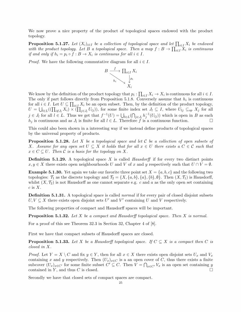
Proposition 5.1.27. Let (Xi)i∈I be a collection of topological space and let∏i∈I Xi be endowed

with the product topology. Let B a topological space. Then a map f : B →∏i∈I Xi is continuous

if and only if hi = pi ◦ f : B → Xi is continuous for all i ∈ I.

Proof. We have the following commutative diagram for all i ∈ I.

B∏i∈I Xi

Xi

f

hipi

We know by the definition of the product topology that pi :∏i∈I Xi → Xi is continuous for all i ∈ I.

The only if part follows directly from Proposition 5.1.8. Conversely assume that hi is continuousfor all i ∈ I. Let U ⊆

∏i∈I Xi be an open subset. Then, by the definition of the product topology,

U =⋃l∈L((

∏i 6∈Jl Xi) × (

∏j∈Jl Ulj)), for some finite index set Jl ⊆ I, where Ulj ⊆op Xj for all

j ∈ Jl for all l ∈ L. Thus we get that f−1(U) =⋃l∈L(

⋂j∈Jl h

−1j (Ulj)) which is open in B as each

hj is continuous and as Jl is finite for all l ∈ L. Therefore f is a continuous function. �

This could also been shown in a interesting way if we instead define products of topological spacesby the universal property of products.

Proposition 5.1.28. Let X be a topological space and let C be a collection of open subsets ofX. Assume for any open set U ⊆ X it holds that for all x ∈ U there exists a C ∈ C such thatx ∈ C ⊆ U . Then C is a basis for the topology on X.

Definition 5.1.29. A topological space X is called Hausdorff if for every two distinct pointsx, y ∈ X there exists open neighbourhoods U and V of x and y respectively such that U ∩ V = ∅.

Example 5.1.30. Yet again we take our favorite three point set X = {a, b, c} and the following twotopologies: T1 as the discrete topology and T2 = {X, {a, b}, {a}, {b}, ∅}. Then (X, T1) is Hausdorff,whilst (X, T2) is not Hausdorff as one cannot separate e.g. c and a as the only open set containingc is X.

Definition 5.1.31. A topological space is called normal if for every pair of closed disjoint subsetsU, V ⊆ X there exists open disjoint sets U ′ and V ′ containing U and V respectively.

The following properties of compact and Hausdorff spaces will be important.

Proposition 5.1.32. Let X be a compact and Hausdorff topological space. Then X is normal.

For a proof of this see Theorem 32.3 in Section 32, Chapter 4 of [8].

First we have that compact subsets of Hausdorff spaces are closed.

Proposition 5.1.33. Let X be a Hausdorff topological space. If C ⊆ X is a compact then C isclosed in X.

Proof. Let Y = X \ C and fix y ∈ Y , then for all x ∈ X there exists open disjoint sets Ux and Vxcontaining x and y respectively. Then (Ux)x∈C is a an open cover of C, thus there exists a finitesubcover (Ux)x∈C′ for some finite subset C ′ ⊆ C. Then V =

⋂x∈C′ Vx is an open set containing y

contained in Y , and thus C is closed. �

Secondly we have that closed sets of compact spaces are compact.25

Proposition 5.1.34. Let X be a compact topological space. If C ⊆ X is a closed subset of X thenC is compact.

Proof. As C is a closed set we get that X \ C is open. Let {Ui}i∈I be any open cover of C. Then{X \ C} ∪ {Ui}i∈I is an open cover of X. Therefore as X is compact there exists a finite subcover{X \C}∪{Uj}j∈J of X for some finite index set J ⊆ I. Then we get that {Uj}j∈J is an open coverof C. Therefore, as {Ui}i∈I was arbitrary, it follows that C is compact. �

The following proposition will be useful for when we want to prove that two spaces are homeomor-phic.

Proposition 5.1.35. If f : X → Y is continuous and bijective map and X is compact and Y isHausdorff, then f is a homeomorphism.

Proof. We will prove this via Proposition 5.1.7. Let U be a closed subset of X then by Propo-sition 5.1.34, U is compact. Then as the image of compact sets are compact we get that f(U)is compact. Then by Proposition 5.1.33 we get that f(U) is closed. Thus f−1 is continuous byProposition 5.1.7 and therefore f is an homeomorphism. �

5.2. Topological Groups. Before we begin studying profinite groups we will need some basicresults about topological groups. The proofs and exposition will follow Chapter III in [2]. Beforewe introduced a topology on a set, but now we instead let the underlying set be a group.

Definition 5.2.1. A topological group is a triple (G, ·, T ) where (G, ·) is a group and (G, T ) is atopological space such that

(i) The map G×G→ G define by (a, b) 7→ ab is continuous.(ii) The map G→ G defined by a 7→ a−1 is continuous.

We then say that the group structure and the topology are compatible on G. We will often, aswith groups and topological spaces, denote a topological group only by its underlying set.

Example 5.2.2. Here are some examples of topological groups

(a) The additive group (Rn,+) is a topological group with the standard topology.(b) Endow C with the standard topology generated by as a basis by all the open balls Br(z),

z ∈ C and r ∈ R. Let T = {z ∈ C | |z| = 1}, that is the unit circle around the origin. Notethat T forms a group under multiplication. If we endow T with the subspace topology givenby the standard topology on C we get that T is a topological group.

We also have following useful proposition for proving that something is a topological group.

Proposition 5.2.3. Let G be a group and let (G, T ) be a topological space. Then G is a topologicalgroup if and only if the map (x, y) 7→ xy−1 is continuous.

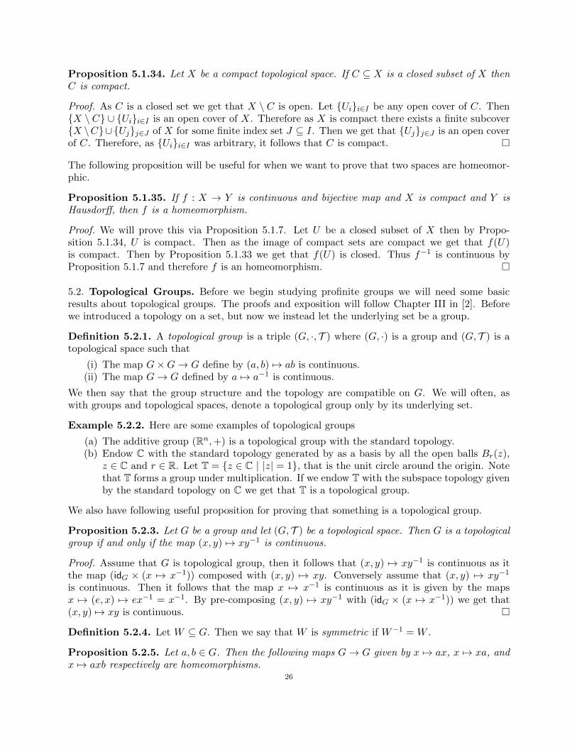
Proof. Assume that G is topological group, then it follows that (x, y) 7→ xy−1 is continuous as itthe map (idG × (x 7→ x−1)) composed with (x, y) 7→ xy. Conversely assume that (x, y) 7→ xy−1

is continuous. Then it follows that the map x 7→ x−1 is continuous as it is given by the mapsx 7→ (e, x) 7→ ex−1 = x−1. By pre-composing (x, y) 7→ xy−1 with (idG × (x 7→ x−1)) we get that(x, y) 7→ xy is continuous. �

Definition 5.2.4. Let W ⊆ G. Then we say that W is symmetric if W−1 = W .

Proposition 5.2.5. Let a, b ∈ G. Then the following maps G→ G given by x 7→ ax, x 7→ xa, andx 7→ axb respectively are homeomorphisms.

26

Proof. From the first condition it follows that the morphism x 7→ ax and x 7→ xa are continuousfor any fixed a, b ∈ G as x 7→ ax and x 7→ xa is equivalent to x 7→ (a, x) 7→ ax and x 7→ (x, a) 7→ xarespectively. It also follows that x 7→ axb is continuous as it is the composition of the two maps x 7→ax and x 7→ xb. Note that especially x 7→ a−1x, x 7→ xa−1 and x 7→ a−1xb−1 are also continuous.Thus the maps x 7→ ax, x 7→ xa, and x 7→ axb for some fixed a, b ∈ G are homeomorphism from Gto G. �

Corollary 5.2.6. Let U ⊆ G be an open neighbourhood of e ∈ G. Then it follows that Ua and aUare open neighbourhoods of a for all a ∈ G. Likewise if V is a open neighbourhood of a ∈ G thena−1V and V a−1 are open neighbourhoods of e ∈ G.

Proof. This follows from Proposition 5.2.5 as Ua is the image of U under the homeomorphismx 7→ xa, thus open. Likewise it follows that aU is a open neighbourhood of x as it is the image of Uunder the homeomorphism x 7→ ax. Now if V is an open neighbourhood of a it follows that a−1Vand V a−1 are open neighbourhoods of e as they are the image of V under the maps x 7→ a−1x andx 7→ xa−1 respectively. �

We therefore have a one to one correspondence between the open neighbourhoods of a point andthe open neighbourhoods of the identity element. Thus it is enough to know what the openneighbourhoods around the identity are to know what the open neighbourhoods around any pointare. For the next proposition we will need to know what a filter is.

Definition 5.2.7. A filter on a set X is a non-empty subset F of the power set of X such thatthe following properties are fulfilled:

(a) If F ⊆ A ⊆ X and F ∈ F , then A ∈ F .(b) If (Ai)i∈I ⊆ F is a finite collection of subsets of F then

⋂i∈I Ai ∈ F .

(c) The empty set is not in F .

We will now also define what a filter base is.

Proposition 5.2.8. Let B be a set of subset of a set X. Then

F = {A ⊆ X | B ⊆ A for some B ∈ B}is a filter if the following condition are fulfilled.

(a) Let A,B ∈ B. Then A ∩B ∈ B.(b) The empty set in not contained in B and B 6= ∅.

Proof. The first condition for begin a filter is fulfilled by F by definition. By induction using (a)the second condition for begin a filter is fulfilled by F . Lastly the last condition for begin a filteris fulfilled by F via (b). �

Definition 5.2.9. A set of subset fulfilling the condition in the above proposition is called a filterbase of F .

Example 5.2.10. If X is topological space, then the collection of all neighbourhoods of a pointx ∈ X is a filter. We call this filter the neighbourhood filter of x. In this case a basis for F is theset of all open sets containing x.

We can now state the next proposition which says that if we have a filter on a group fulfillingcertain condition then this filter induces a compatible topology on this group where the filter isprecisely the neighbourhood filter of e.

Proposition 5.2.11. Let G be a group and let F be a filter fulfilling the following properties:

(a) Let U ∈ F , then there exists a V ∈ F such that V · V ⊆ U(b) Let U ∈ F , then U−1 ∈ F .

27

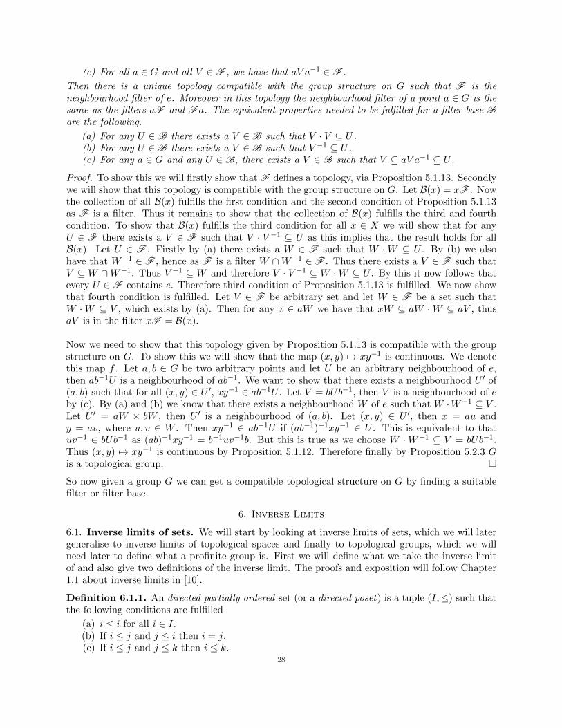
(c) For all a ∈ G and all V ∈ F , we have that aV a−1 ∈ F .

Then there is a unique topology compatible with the group structure on G such that F is theneighbourhood filter of e. Moreover in this topology the neighbourhood filter of a point a ∈ G is thesame as the filters aF and Fa. The equivalent properties needed to be fulfilled for a filter base Bare the following.

(a) For any U ∈ B there exists a V ∈ B such that V · V ⊆ U .(b) For any U ∈ B there exists a V ∈ B such that V −1 ⊆ U .(c) For any a ∈ G and any U ∈ B, there exists a V ∈ B such that V ⊆ aV a−1 ⊆ U .

Proof. To show this we will firstly show that F defines a topology, via Proposition 5.1.13. Secondlywe will show that this topology is compatible with the group structure on G. Let B(x) = xF . Nowthe collection of all B(x) fulfills the first condition and the second condition of Proposition 5.1.13as F is a filter. Thus it remains to show that the collection of B(x) fulfills the third and fourthcondition. To show that B(x) fulfills the third condition for all x ∈ X we will show that for anyU ∈ F there exists a V ∈ F such that V · V −1 ⊆ U as this implies that the result holds for allB(x). Let U ∈ F . Firstly by (a) there exists a W ∈ F such that W ·W ⊆ U . By (b) we alsohave that W−1 ∈ F , hence as F is a filter W ∩W−1 ∈ F . Thus there exists a V ∈ F such thatV ⊆ W ∩W−1. Thus V −1 ⊆ W and therefore V · V −1 ⊆ W ·W ⊆ U . By this it now follows thatevery U ∈ F contains e. Therefore third condition of Proposition 5.1.13 is fulfilled. We now showthat fourth condition is fulfilled. Let V ∈ F be arbitrary set and let W ∈ F be a set such thatW ·W ⊆ V , which exists by (a). Then for any x ∈ aW we have that xW ⊆ aW ·W ⊆ aV , thusaV is in the filter xF = B(x).

Now we need to show that this topology given by Proposition 5.1.13 is compatible with the groupstructure on G. To show this we will show that the map (x, y) 7→ xy−1 is continuous. We denotethis map f . Let a, b ∈ G be two arbitrary points and let U be an arbitrary neighbourhood of e,then ab−1U is a neighbourhood of ab−1. We want to show that there exists a neighbourhood U ′ of(a, b) such that for all (x, y) ∈ U ′, xy−1 ∈ ab−1U . Let V = bUb−1, then V is a neighbourhood of eby (c). By (a) and (b) we know that there exists a neighbourhood W of e such that W ·W−1 ⊆ V .Let U ′ = aW × bW , then U ′ is a neighbourhood of (a, b). Let (x, y) ∈ U ′, then x = au andy = av, where u, v ∈ W . Then xy−1 ∈ ab−1U if (ab−1)−1xy−1 ∈ U . This is equivalent to thatuv−1 ∈ bUb−1 as (ab)−1xy−1 = b−1uv−1b. But this is true as we choose W ·W−1 ⊆ V = bUb−1.Thus (x, y) 7→ xy−1 is continuous by Proposition 5.1.12. Therefore finally by Proposition 5.2.3 Gis a topological group. �

So now given a group G we can get a compatible topological structure on G by finding a suitablefilter or filter base.

6. Inverse Limits

6.1. Inverse limits of sets. We will start by looking at inverse limits of sets, which we will latergeneralise to inverse limits of topological spaces and finally to topological groups, which we willneed later to define what a profinite group is. First we will define what we take the inverse limitof and also give two definitions of the inverse limit. The proofs and exposition will follow Chapter1.1 about inverse limits in [10].

Definition 6.1.1. An directed partially ordered set (or a directed poset) is a tuple (I,≤) such thatthe following conditions are fulfilled

(a) i ≤ i for all i ∈ I.(b) If i ≤ j and j ≤ i then i = j.(c) If i ≤ j and j ≤ k then i ≤ k.

28

(d) For all i, j ∈ I there exists a k ∈ I such that i ≤ k and j ≤ k.

We will say poset instead of partially ordered set and we will often denote a directed poset only byits underlying set.

Definition 6.1.2. An inverse system over an directed partially ordered set I is a double (Ai, ϕij),where the Ai’s are sets and ϕij : Aj → Ai, ϕii = idAi are maps between the sets, such that thefollowing diagram commutes for any i ≤ j ≤ k

Aj

Ai Ak

ϕij ϕjk

ϕik

Now there are so to say two definitions of the inverse limit of an inverse system, one is moreconcrete, whilst one is the more abstract definition. We will first give the concrete definition andafter that give the abstract definition. Then finally we will prove that the concrete definition isindeed a inverse limit in the abstract sense.

Definition 6.1.3. Let (Ai, ϕij) be an inverse system over a directed poset I. The inverse limitA = lim←−Ai of (Ai, ϕij) is the following subset of the set

∏i∈I Ai,

lim←−Ai = {a ∈∏i∈I

Ai | ai = ϕij(aj) for all i ≤ j in I}.

Note that we will only use lim←−Ai to refer to the set above and not to the inverse limit in the abstractsense.

Informally one can of think of this construction kind of like when construction the real numbersone “completes” the rational numbers by taking all Cauchy sequences of rational numbers.

Example 6.1.4. The simplest example is the case where one has the inverse system over andirected poset I consisting of sets (Xi,⊆) looking as X0 ⊇ X1 ⊇ ... ⊇ Xi ⊇ Xi+1 ⊇ ..., where themaps are all inclusions. Then we get that lim←−Xi =

⋂i∈I Xi. So in some sense inverse limits are

like generalised intersections. The inverse limit can be seen as the smallest object we can “glue”together from the objects that we take the inverse limit of.

Example 6.1.5. Given any set A we can always define the constant inverse system (A, idA) overan arbitrary directed poset I consisting only of A’s and identity maps between them for any indexset I. For example if we take I to be equal to N it looks like this (a bit misleading in general asthe A’s need not lie in a straight line for a arbitrary index set I)

A A A A A ...idA idA idA idA idA

In these cases we simply get that lim←−A = A.

We will now give the more abstract definition of an inverse limit. This kind of construction isgenerally not the first imagined. Instead this is the definition we get if translate properties ofobjects into properties of morphism and objects.

Definition 6.1.6. Let (Ai, ϕij) be an inverse system over an directed poset I. We say that (A,ϕi),where ϕi : A→ Ai, is a cone over (Ai, ϕij) if the following diagram commutes for all i ≤ j

A

Ai Aj

ϕjϕi

ϕij

29

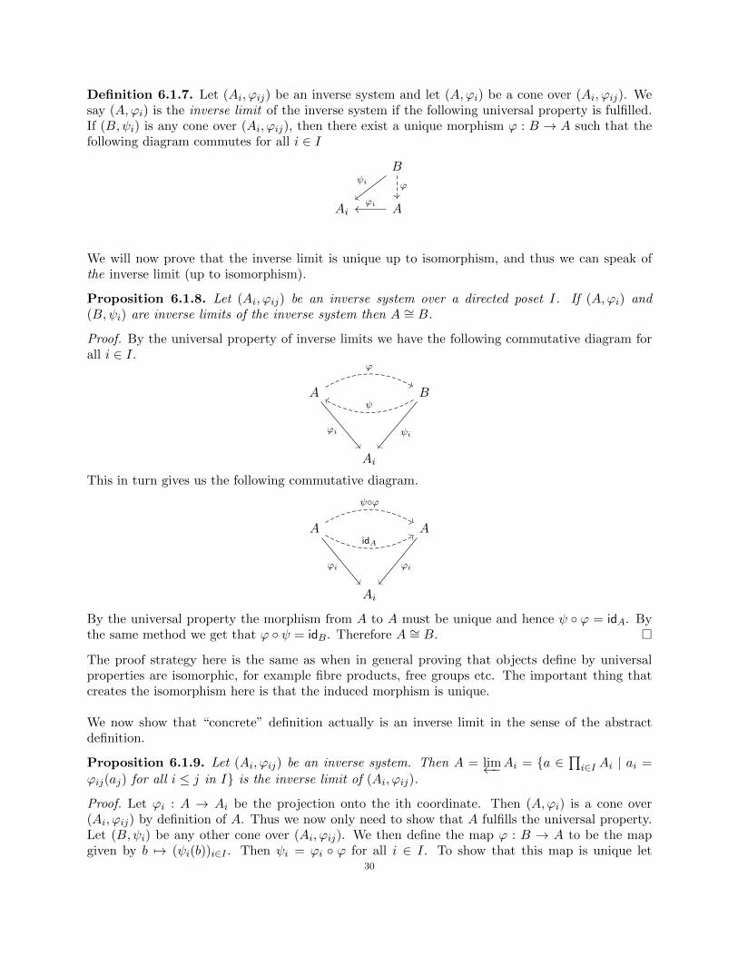
Definition 6.1.7. Let (Ai, ϕij) be an inverse system and let (A,ϕi) be a cone over (Ai, ϕij). Wesay (A,ϕi) is the inverse limit of the inverse system if the following universal property is fulfilled.If (B,ψi) is any cone over (Ai, ϕij), then there exist a unique morphism ϕ : B → A such that thefollowing diagram commutes for all i ∈ I

B

Ai A

ϕψi

ϕi

We will now prove that the inverse limit is unique up to isomorphism, and thus we can speak ofthe inverse limit (up to isomorphism).

Proposition 6.1.8. Let (Ai, ϕij) be an inverse system over a directed poset I. If (A,ϕi) and(B,ψi) are inverse limits of the inverse system then A ∼= B.

Proof. By the universal property of inverse limits we have the following commutative diagram forall i ∈ I.

A B

Ai

ϕ

ϕi

ψ

ψi

This in turn gives us the following commutative diagram.

A A

Ai

ψ◦ϕ

idA

ϕi ϕi

By the universal property the morphism from A to A must be unique and hence ψ ◦ ϕ = idA. Bythe same method we get that ϕ ◦ ψ = idB. Therefore A ∼= B. �

The proof strategy here is the same as when in general proving that objects define by universalproperties are isomorphic, for example fibre products, free groups etc. The important thing thatcreates the isomorphism here is that the induced morphism is unique.

We now show that “concrete” definition actually is an inverse limit in the sense of the abstractdefinition.

Proposition 6.1.9. Let (Ai, ϕij) be an inverse system. Then A = lim←−Ai = {a ∈∏i∈I Ai | ai =

ϕij(aj) for all i ≤ j in I} is the inverse limit of (Ai, ϕij).

Proof. Let ϕi : A → Ai be the projection onto the ith coordinate. Then (A,ϕi) is a cone over(Ai, ϕij) by definition of A. Thus we now only need to show that A fulfills the universal property.Let (B,ψi) be any other cone over (Ai, ϕij). We then define the map ϕ : B → A to be the mapgiven by b 7→ (ψi(b))i∈I . Then ψi = ϕi ◦ ϕ for all i ∈ I. To show that this map is unique let

30

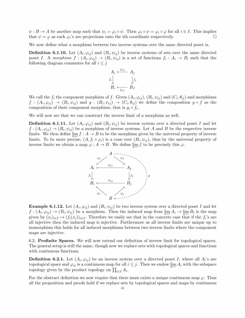
ψ : B → A be another map such that ψi = ϕi ◦ ψ. Then ϕi ◦ ψ = ϕi ◦ ϕ for all i ∈ I. This impliesthat ψ = ϕ as each ϕi’s are projections onto the ith coordinate respectively. �

We now define what a morphism between two inverse systems over the same directed poset is.

Definition 6.1.10. Let (Ai, ϕij) and (Bi, ψij) be inverse systems of sets over the same directedposet I. A morphism f : (Ai, ϕij) → (Bi, ψij) is a set of functions fi : Ai → Bi such that thefollowing diagram commutes for all i ≤ j

Ai Aj

Bi BJ

fi fj

ϕij

ψij

We call the fi the component morphism of f . Given (Ai, ϕij), (Bi, ψij) and (Ci, θij) and morphismsf : (Ai, ϕij) → (Bi, ψij) and g : (Bi, ψij) → (Ci, θij) we define the composition g ◦ f as thecomposition of their component morphism, that is gi ◦ fi.

We will now see that we can construct the inverse limit of a morphism as well.

Definition 6.1.11. Let (Ai, ϕij) and (Bi, ψij) be inverse system over a directed poset I and letf : (Ai, ϕij)→ (Bi, ψij) be a morphism of inverse systems. Let A and B be the respective inverselimits. We then define lim←− f : A→ B to be the morphism given by the universal property of inverse

limits. To be more precise, (A, fi ◦ ϕi) is a cone over (Bi, ψij), thus by the universal property ofinverse limits we obtain a map ϕ : A→ B. We define lim←− f to be precisely this ϕ.

A

Ai Aj

Bi Bj

B

ϕ

ϕi ϕj

fi

ϕij

fj

ψij

ψi ψj

Example 6.1.12. Let (Ai, ϕij) and (Bi, ψij) be two inverse system over a directed poset I and letf : (Ai, ϕij) → (Bi, ψij) be a morphism. Then the induced map from lim←−Ai → lim←−Bi is the map

given by (xi)i∈I 7→ (fi(xi))i∈I . Therefore we easily see that in the concrete case that if the fi’s areall injective then the induced map is injective. Furthermore as all inverse limits are unique up toisomorphism this holds for all induced morphisms between two inverse limits where the componentmaps are injective.

6.2. Profinite Spaces. We will now extend our definition of inverse limit for topological spaces.The general setup is still the same, though now we replace sets with topological spaces and functionswith continuous functions.

Definition 6.2.1. Let (Ai, ϕij) be an inverse system over a directed poset I, where all Ai’s aretopological space and ϕij is a continuous map for all i ≤ j. Then we endow lim←−Ai with the subspace

topology given by the product topology on∏i∈I Ai.

For the abstract definition we now require that there must exists a unique continuous map ϕ. Thusall the proposition and proofs hold if we replace sets by topological spaces and maps by continuous

31

maps except we need to show that the map given in the proof of Proposition 6.1.9 is continuous.We now restate and proof the Proposition for topological spaces.

Proposition 6.2.2. Let (Ai, ϕij) be an inverse system of topological spaces over a directed poset I.Then A = lim←−Ai = {a ∈

∏i∈I Ai | ai = ϕij(aj) for all i ≤ j in I} is the inverse limit of (Ai, ϕij).

Proof. Let (B,ψi) be any other compatible topological space. Then define the map f : B → A tobe the map given by b 7→ (ψi(b))i∈I . Now we only need to show that f is continuous as the restfollows by the proof of Proposition 6.1.9. Let V be an open set in A, then

V = A ∩

⋃l∈L

∏i 6∈Jl

Ai ×∏j∈Jl

Ulj

where Jl ⊆ I is a finite subset for all l ∈ L and Ulj ⊆ Aj is open for all j ∈ J and all l ∈ L. Then

f−1(V ) = B ∩

⋃l∈L

⋂j∈Jl

ψ−1j (Ulj)

which is open in B as Jl is finite for all l ∈ L and each ψ−1j (Ulj) is open as each ψj is continuous.Thus f is a continuous function. �

For this section we only prove all results for the concrete inverse limit, lim←−Ai, but as the inverselimit is unique up to isomorphism this implies that the results hold in general.

Proposition 6.2.3. Let (Ai, ϕij) be an inverse system of Hausdorff topological spaces over a di-rected poset I. Then lim←−Ai is closed subset of

∏i∈I Ai.

Proof. To prove this we will show that∏i∈I Ai \ lim←−Ai is an open set. Let B =

∏i∈I Ai \ lim←−Ai

and let (ai)i∈I ∈ B. Then there exists i, j such that i < j but ϕij(aj) 6= ai. As Ai is Hausdorffthere exists open neighbourhoods U and V of ϕij(aj) and ai such that U ∩ V = ∅. Let U ′ be anopen neighbourhood of aj in Aj such that ϕij(U

′) ⊆ U . Such a neighbourhood exists as we can

for example pick U ′ = ϕ−1ij (U). Consider the open set W =∏k∈I Vi where Vi = V , Vj = U ′ and

Vk = Xk for all k 6= i, j. Assume (towards a contradiction) that there exists a bj ∈ U ′ such thatϕij(bj) = bi ∈ V . Then this would contradict that U ∩ V = ∅ and therefore W is an open setcontaining (ai)i∈I contained in B. Thus B is open and therefore lim←−Ai is closed. �

To prove this next proposition we will need Tychnoff’s theorem. Unfortunately we won’t be able toprove it here, so therefore we will have to take it as a black box. For a proof of Tychnoff’s theoremsee for example Chapter 5 in [8].

Theorem 6.2.4 (Tychnoff’s theorem). Let (Ai)i∈I be a collection of compact spaces, then∏i∈I Ai

is a compact space.

We will now see how some topological properties transfer to the inverse limit from the inversesystem.

Proposition 6.2.5. Let (Ai, ϕij) be an inverse system over a directed poset I. Then if every Ai iscompact, Hausdorff and totally disconnected then the inverse limit lim←−i∈I Ai is compact, Hausdorff

and totally disconnected.

Proof. Let A = lim←−Ai. By Tychnoff’s theorem we get that∏i∈I Ai is compact as each Ai is

compact. This in turn implies that lim←−Ai is compact by Proposition 5.1.34, as by Proposition 6.2.3

lim←−Ai is a closed subset of∏i∈I Ai. Now we show that A is Hausdorff. It is enough to show

that∏i∈I Ai is Hausdorff as then the induced subspace topology will be Hausdorff as well. Let

32

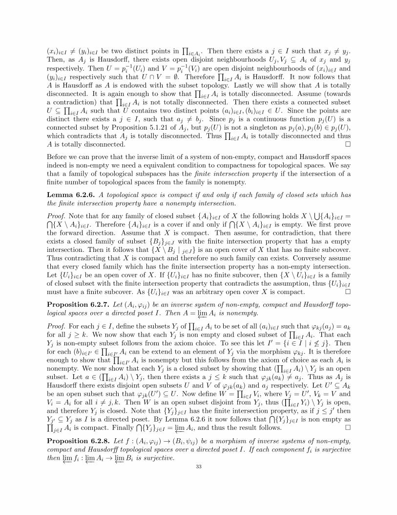
(xi)i∈I 6= (yi)i∈I be two distinct points in∏i∈Ai . Then there exists a j ∈ I such that xj 6= yj .

Then, as Aj is Hausdorff, there exists open disjoint neighbourhoods Uj , Vj ⊆ Ai of xj and yjrespectively. Then U = p−1i (Ui) and V = p−1i (Vi) are open disjoint neighbourhoods of (xi)i∈I and(yi)i∈I respectively such that U ∩ V = ∅. Therefore

∏i∈I Ai is Hausdorff. It now follows that

A is Hausdorff as A is endowed with the subset topology. Lastly we will show that A is totallydisconnected. It is again enough to show that

∏i∈I Ai is totally disconnected. Assume (towards

a contradiction) that∏i∈I Ai is not totally disconnected. Then there exists a connected subset

U ⊆∏i∈I Ai such that U contains two distinct points (ai)i∈I , (bi)i∈I ∈ U . Since the points are

distinct there exists a j ∈ I, such that aj 6= bj . Since pj is a continuous function pj(U) is aconnected subset by Proposition 5.1.21 of Aj , but pj(U) is not a singleton as pj(a), pj(b) ∈ pj(U),which contradicts that Aj is totally disconnected. Thus

∏i∈I Ai is totally disconnected and thus

A is totally disconnected. �

Before we can prove that the inverse limit of a system of non-empty, compact and Hausdorff spacesindeed is non-empty we need a equivalent condition to compactness for topological spaces. We saythat a family of topological subspaces has the finite intersection property if the intersection of afinite number of topological spaces from the family is nonempty.

Lemma 6.2.6. A topological space is compact if and only if each family of closed sets which hasthe finite intersection property have a nonempty intersection.

Proof. Note that for any family of closed subset {Ai}i∈I of X the following holds X \⋃{Ai}i∈I =⋂

{X \ Ai}i∈I . Therefore {Ai}i∈I is a cover if and only if⋂{X \ Ai}i∈I is empty. We first prove

the forward direction. Assume that X is compact. Then assume, for contradiction, that thereexists a closed family of subset {Bj}j∈J with the finite intersection property that has a emptyintersection. Then it follows that {X \Bj | j∈J} is an open cover of X that has no finite subcover.Thus contradicting that X is compact and therefore no such family can exists. Conversely assumethat every closed family which has the finite intersection property has a non-empty intersection.Let {Ui}i∈I be an open cover of X. If {Ui}i∈I has no finite subcover, then {X \ Ui}i∈I is a familyof closed subset with the finite intersection property that contradicts the assumption, thus {Ui}i∈Imust have a finite subcover. As {Ui}i∈I was an arbitrary open cover X is compact. �

Proposition 6.2.7. Let (Ai, ϕij) be an inverse system of non-empty, compact and Hausdorff topo-logical spaces over a directed poset I. Then A = lim←−Ai is nonempty.

Proof. For each j ∈ I, define the subsets Yj of∏i∈I Ai to be set of all (ai)i∈I such that ϕkj(aj) = ak

for all j ≥ k. We now show that each Yj is non empty and closed subset of∏i∈I Ai. That each

Yj is non-empty subset follows from the axiom choice. To see this let I ′ = {i ∈ I | i 6≤ j}. Thenfor each (b)i∈I′ ∈

∏i∈I′ Ai can be extend to an element of Yj via the morphism ϕkj . It is therefore

enough to show that∏i∈I′ Ai is nonempty but this follows from the axiom of choice as each Ai is

nonempty. We now show that each Yj is a closed subset by showing that (∏i∈I Ai) \ Yj is an open

subset. Let a ∈ (∏i∈I Ai) \ Yj , then there exists a j ≤ k such that ϕjk(ak) 6= aj . Thus as Aj is

Hausdorff there exists disjoint open subsets U and V of ϕjk(ak) and aj respectively. Let U ′ ⊆ Akbe an open subset such that ϕjk(U

′) ⊆ U . Now define W =∏i∈I Vi, where Vj = U ′, Vk = V and

Vi = Ai for all i 6= j, k. Then W is an open subset disjoint from Yj , thus (∏i∈I Yi) \ Yj is open,

and therefore Yj is closed. Note that {Yj}j∈I has the finite intersection property, as if j ≤ j′ thenYj′ ⊆ Yj as I is a directed poset. By Lemma 6.2.6 it now follows that

⋂{Yj}j∈I is non empty as∏

j∈I Ai is compact. Finally⋂{Yj}j∈I = lim←−Ai, and thus the result follows. �

Proposition 6.2.8. Let f : (Ai, ϕij)→ (Bi, ψij) be a morphism of inverse systems of non-empty,compact and Hausdorff topological spaces over a directed poset I. If each component fi is surjectivethen lim←− fi : lim←−Ai → lim←−Bi is surjective.

33

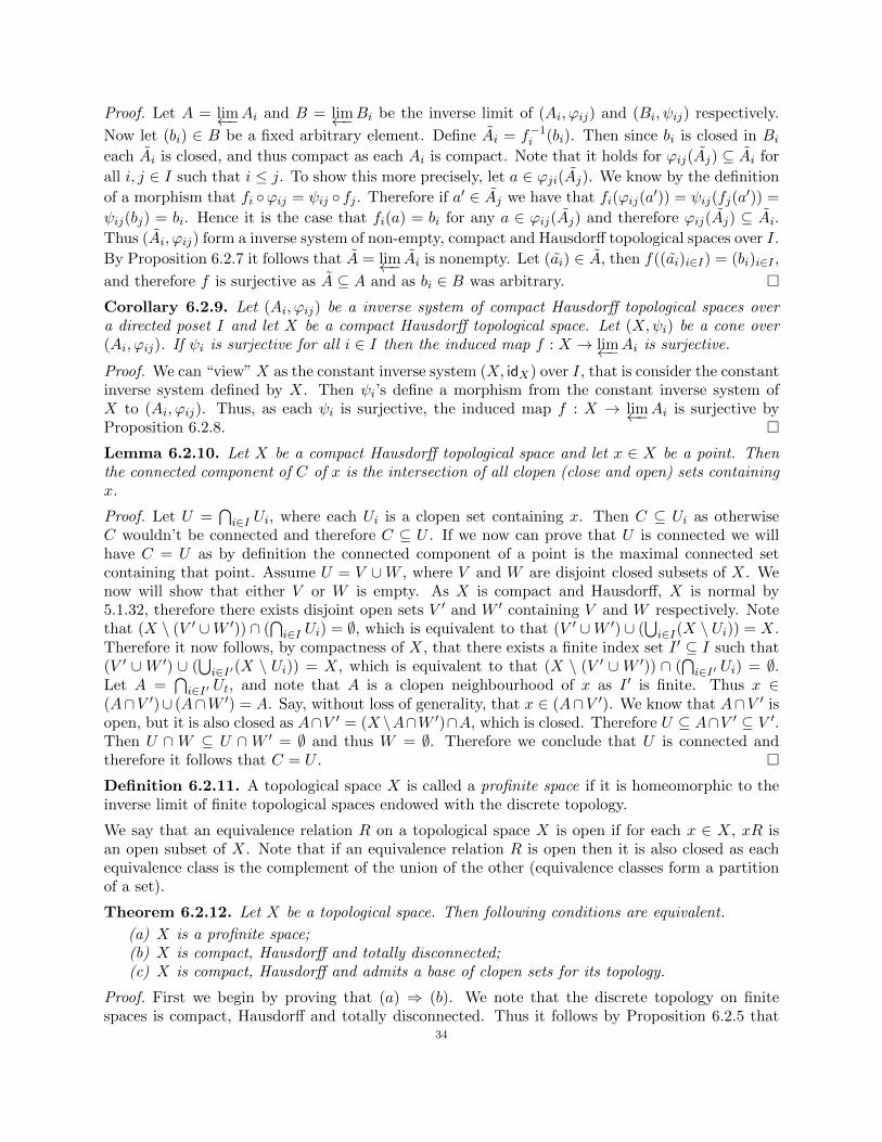
Proof. Let A = lim←−Ai and B = lim←−Bi be the inverse limit of (Ai, ϕij) and (Bi, ψij) respectively.

Now let (bi) ∈ B be a fixed arbitrary element. Define Ai = f−1i (bi). Then since bi is closed in Bieach Ai is closed, and thus compact as each Ai is compact. Note that it holds for ϕij(Aj) ⊆ Ai for

all i, j ∈ I such that i ≤ j. To show this more precisely, let a ∈ ϕji(Aj). We know by the definition

of a morphism that fi ◦ϕij = ψij ◦ fj . Therefore if a′ ∈ Aj we have that fi(ϕij(a′)) = ψij(fj(a

′)) =

ψij(bj) = bi. Hence it is the case that fi(a) = bi for any a ∈ ϕij(Aj) and therefore ϕij(Aj) ⊆ Ai.

Thus (Ai, ϕij) form a inverse system of non-empty, compact and Hausdorff topological spaces over I.

By Proposition 6.2.7 it follows that A = lim←− Ai is nonempty. Let (ai) ∈ A, then f((ai)i∈I) = (bi)i∈I ,

and therefore f is surjective as A ⊆ A and as bi ∈ B was arbitrary. �

Corollary 6.2.9. Let (Ai, ϕij) be a inverse system of compact Hausdorff topological spaces overa directed poset I and let X be a compact Hausdorff topological space. Let (X,ψi) be a cone over(Ai, ϕij). If ψi is surjective for all i ∈ I then the induced map f : X → lim←−Ai is surjective.

Proof. We can “view” X as the constant inverse system (X, idX) over I, that is consider the constantinverse system defined by X. Then ψi’s define a morphism from the constant inverse system ofX to (Ai, ϕij). Thus, as each ψi is surjective, the induced map f : X → lim←−Ai is surjective byProposition 6.2.8. �

Lemma 6.2.10. Let X be a compact Hausdorff topological space and let x ∈ X be a point. Thenthe connected component of C of x is the intersection of all clopen (close and open) sets containingx.

Proof. Let U =⋂i∈I Ui, where each Ui is a clopen set containing x. Then C ⊆ Ui as otherwise

C wouldn’t be connected and therefore C ⊆ U . If we now can prove that U is connected we willhave C = U as by definition the connected component of a point is the maximal connected setcontaining that point. Assume U = V ∪W , where V and W are disjoint closed subsets of X. Wenow will show that either V or W is empty. As X is compact and Hausdorff, X is normal by5.1.32, therefore there exists disjoint open sets V ′ and W ′ containing V and W respectively. Notethat (X \ (V ′ ∪W ′)) ∩ (

⋂i∈I Ui) = ∅, which is equivalent to that (V ′ ∪W ′) ∪ (

⋃i∈I(X \ Ui)) = X.

Therefore it now follows, by compactness of X, that there exists a finite index set I ′ ⊆ I such that(V ′ ∪W ′) ∪ (

⋃i∈I′(X \ Ui)) = X, which is equivalent to that (X \ (V ′ ∪W ′)) ∩ (

⋂i∈I′ Ui) = ∅.

Let A =⋂i∈I′ Ut, and note that A is a clopen neighbourhood of x as I ′ is finite. Thus x ∈

(A∩V ′)∪ (A∩W ′) = A. Say, without loss of generality, that x ∈ (A∩V ′). We know that A∩V ′ isopen, but it is also closed as A∩V ′ = (X \A∩W ′)∩A, which is closed. Therefore U ⊆ A∩V ′ ⊆ V ′.Then U ∩W ⊆ U ∩W ′ = ∅ and thus W = ∅. Therefore we conclude that U is connected andtherefore it follows that C = U . �

Definition 6.2.11. A topological space X is called a profinite space if it is homeomorphic to theinverse limit of finite topological spaces endowed with the discrete topology.

We say that an equivalence relation R on a topological space X is open if for each x ∈ X, xR isan open subset of X. Note that if an equivalence relation R is open then it is also closed as eachequivalence class is the complement of the union of the other (equivalence classes form a partitionof a set).

Theorem 6.2.12. Let X be a topological space. Then following conditions are equivalent.

(a) X is a profinite space;(b) X is compact, Hausdorff and totally disconnected;(c) X is compact, Hausdorff and admits a base of clopen sets for its topology.

Proof. First we begin by proving that (a) ⇒ (b). We note that the discrete topology on finitespaces is compact, Hausdorff and totally disconnected. Thus it follows by Proposition 6.2.5 that

34

X is compact, Hausdorff and totally disconnected.

We now prove that (b) ⇒ (c). By Proposition 5.1.28 the result follows if we can prove thatgiven any open subset U of X, there exists a clopen set C such that x ∈ C ⊆ U for all x ∈ U .Let U be any open subset of X and let x ∈ U be an arbitrary point. Let C =

⋂t∈T Ct be the

intersection of all clopen neighbourhoods of x. By Lemma 6.2.10 it follows that⋂t∈T Ct = {x}. As

X \ U is closed set disjoint from C it follows by compactness of X that there exists a finite subsetT ′ of T such that (X \ U) ∩ (

⋂t∈T ′ Ct) = ∅ as this is equivalent to that U ∪ (

⋃t∈T (X \ Ut)) = X

has a finite subcover. Thus⋂t∈T ′ Ct is a clopen set containing x that is contained in U .

We finally prove that (c) ⇒ (a). Let R denote the collection of all open equivalence classeson X. Note that X/R will be a finite and discrete topological space for any R ∈ R as X is com-pact. Define a order ≤ on R by that R1 ≤ R2 if for all x ∈ X, xR2 ⊆ xR1. One easily sees that(R,≤) is partially ordered set. To see that it is also directed note that for any R1, R2 ∈ R, itholds that R1, R2 ≤ R1 ∩ R2. If R1 ≤ R2 we can define the map ϕR1R2 : X/R2 → X/R1 given byϕR1R2(xR2) = xR1 for all x ∈ X. Note that if R1 ≤ R2 ≤ R3 the following diagram commutes.

X/R1 X/R3

X/R2

ϕR1R3

ϕR2R3ϕR1R2

Therefore we get that (X/R,ϕRR′) forms an inverse system of topological spaces over R. Thus wecan define Y = lim←−R∈RX/R. We want to show that X ∼= Y . We first define the map fR : X → X/R

by fR(x) = xR. Next define f : X → Y to be the map lim←− fR. By Corollary 6.2.9 it follows thatf is surjective as each fR is, thus we only need to show that f is injective as then f will bean isomorphism as X is compact. Let x, y ∈ X be two distinct points. Then there exists aclopen set U containing x but not y as X is Hausdorff and admits a base of clopen sets for itstopology. Now consider the open equivalence relation RU given by the partition X − U and U .Then fRU (x) 6= fRU (y), thus f(x) 6= f(y) as fR = f ◦ ϕR. Therefore f is injective and thusbijective. �

7. Profinite Groups and Galois Extensions

In this section we will first define what a profinite group is and give a characterisation of profinitegroups as well as some basic properties. Then we will show that every Galois group is a profinitegroup and that every profinite group can be seen as a Galois group. The proofs and exposition willfollow Chapter 2 in [10].

7.1. Profinite Groups. Before we can define what a profinite group is we need to extend ourdefinition of inverse limits to topological groups. To do this we just replace the topological spacesby topological groups and the continuous maps by continuous morphisms. All the proofs in theprevious section hold for topological groups except we need to show that the concrete definition isalso an inverse limit for topological groups. We now restate Proposition 6.2.2 in terms of topologicalgroups.

Proposition 7.1.1. Let (Ai, ϕij) be an inverse system of topological groups. Then A = lim←−Ai =

{a ∈∏i∈I Ai | ai = ϕij(aj) for all i ≤ j in I} is the inverse limit of (Ai, ϕij).

35

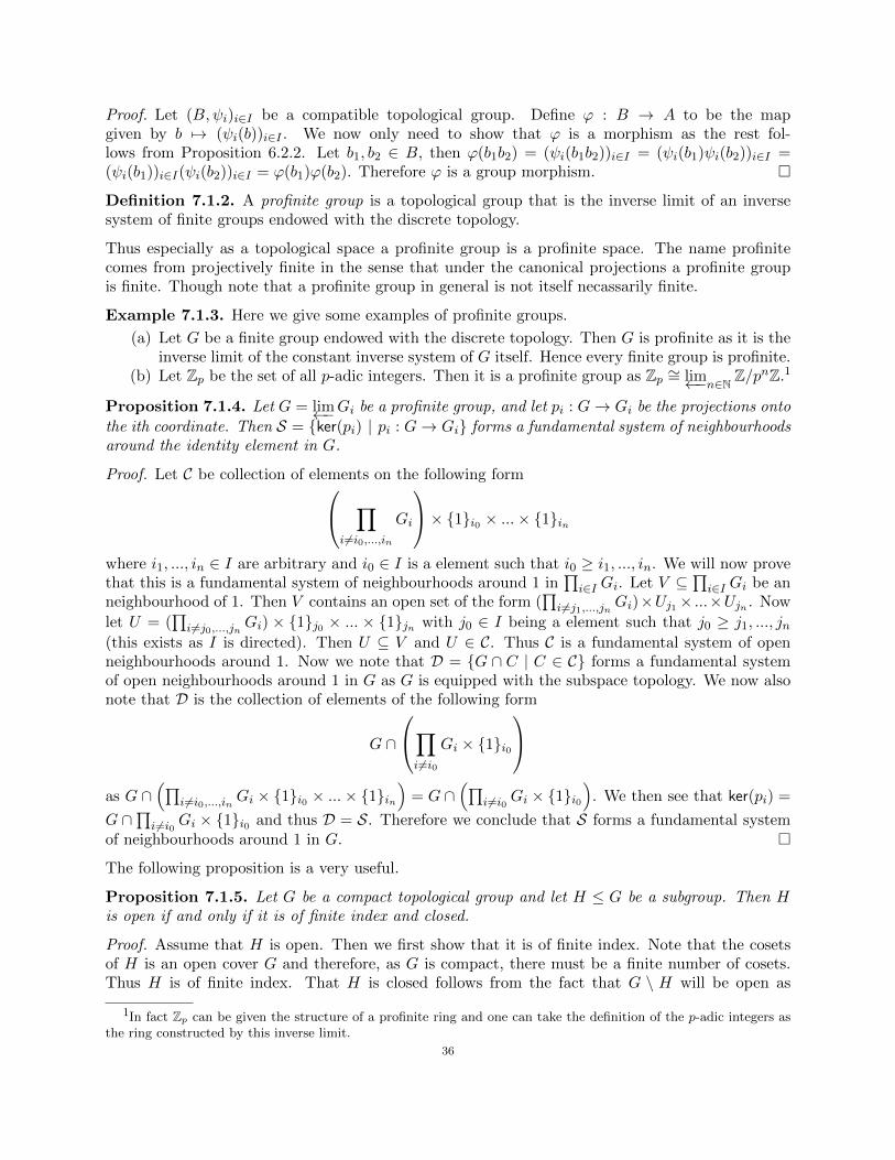
Proof. Let (B,ψi)i∈I be a compatible topological group. Define ϕ : B → A to be the mapgiven by b 7→ (ψi(b))i∈I . We now only need to show that ϕ is a morphism as the rest fol-lows from Proposition 6.2.2. Let b1, b2 ∈ B, then ϕ(b1b2) = (ψi(b1b2))i∈I = (ψi(b1)ψi(b2))i∈I =(ψi(b1))i∈I(ψi(b2))i∈I = ϕ(b1)ϕ(b2). Therefore ϕ is a group morphism. �

Definition 7.1.2. A profinite group is a topological group that is the inverse limit of an inversesystem of finite groups endowed with the discrete topology.

Thus especially as a topological space a profinite group is a profinite space. The name profinitecomes from projectively finite in the sense that under the canonical projections a profinite groupis finite. Though note that a profinite group in general is not itself necassarily finite.

Example 7.1.3. Here we give some examples of profinite groups.

(a) Let G be a finite group endowed with the discrete topology. Then G is profinite as it is theinverse limit of the constant inverse system of G itself. Hence every finite group is profinite.

(b) Let Zp be the set of all p-adic integers. Then it is a profinite group as Zp ∼= lim←−n∈N Z/pnZ.1

Proposition 7.1.4. Let G = lim←−Gi be a profinite group, and let pi : G→ Gi be the projections onto

the ith coordinate. Then S = {ker(pi) | pi : G→ Gi} forms a fundamental system of neighbourhoodsaround the identity element in G.

Proof. Let C be collection of elements on the following form ∏i 6=i0,...,in

Gi

× {1}i0 × ...× {1}inwhere i1, ..., in ∈ I are arbitrary and i0 ∈ I is a element such that i0 ≥ i1, ..., in. We will now provethat this is a fundamental system of neighbourhoods around 1 in

∏i∈I Gi. Let V ⊆

∏i∈I Gi be an

neighbourhood of 1. Then V contains an open set of the form (∏i 6=j1,...,jn Gi)×Uj1× ...×Ujn . Now

let U = (∏i 6=j0,...,jn Gi) × {1}j0 × ... × {1}jn with j0 ∈ I being a element such that j0 ≥ j1, ..., jn

(this exists as I is directed). Then U ⊆ V and U ∈ C. Thus C is a fundamental system of openneighbourhoods around 1. Now we note that D = {G ∩ C | C ∈ C} forms a fundamental systemof open neighbourhoods around 1 in G as G is equipped with the subspace topology. We now alsonote that D is the collection of elements of the following form

G ∩

∏i 6=i0

Gi × {1}i0

as G ∩

(∏i 6=i0,...,in Gi × {1}i0 × ...× {1}in

)= G ∩

(∏i 6=i0 Gi × {1}i0

). We then see that ker(pi) =

G ∩∏i 6=i0 Gi × {1}i0 and thus D = S. Therefore we conclude that S forms a fundamental system

of neighbourhoods around 1 in G. �

The following proposition is a very useful.

Proposition 7.1.5. Let G be a compact topological group and let H ≤ G be a subgroup. Then His open if and only if it is of finite index and closed.

Proof. Assume that H is open. Then we first show that it is of finite index. Note that the cosetsof H is an open cover G and therefore, as G is compact, there must be a finite number of cosets.Thus H is of finite index. That H is closed follows from the fact that G \ H will be open as

1In fact Zp can be given the structure of a profinite ring and one can take the definition of the p-adic integers asthe ring constructed by this inverse limit.

36

G \ H =⋃gH 6=H gH as gH is open for all g ∈ G by Proposition 5.2.5. Conversely assume that

H is a closed subgroup of finite index. Let G′ ⊆ G be the index set of the left cosets. Then byProposition 5.2.5 we get that g′H is closed for all g′ ∈ G′. Therefore N =

⋃g′ 6=e g

′H is closed.

Then finally H is open as H = G \N . �

Before we can prove the following theorem we need the following useful lemma.

Lemma 7.1.6. Let G be a compact topological group and let H ≤ G be a open subgroup. Then thecore of H, defined as core(H) =

⋂g∈G gHg

−1, is an open subgroup.

Proof. This follows from Proposition 7.1.5 as H is open which implies that H has finite index. LetG′ ⊆ G be an index set for the cosets of H. Note that gHg−1 = hHh−1 if g and h lie in the samecoset. Therefore we get that core(H) =

⋂g∈G′ gHg−1 is open as gHg−1 is open for all g ∈ G′ by

Proposition 5.2.5 and since G′ is finite. �

We will now give a characterisation of profinite groups analog to Theorem 6.2.12.

Theorem 7.1.7. The following condition on a topological group G are equivalent.

(a) G is a profinite group(b) G is compact, Hausdorff and totally disconnected.(c) G is compact, Hausdorff and the identity element 1 of G admits a fundamental system S

of open subgroups U satisfying⋂U∈S U = {1} and U EG with G/U finite.

(d) The identity element 1 of G admits a fundamental system S of open neighbourhoods Usatisfying U EG for all U ∈ S, with G/U being finite, and G = lim←−U∈S G/U .

Proof. (a) ⇒ (b):It follows directly from Theorem 6.2.12 that G is compact, Hausdorff and totally disconnected.

(b) ⇒ (c):By assumption we already have that G is compact and Hausdorff. We know by Theorem 6.2.12that G admits a basis of clopen sets C. Thus, we have a fundamental system of clopen sets aroundeach point and therefore especially around 1. Denote this fundamental system around 1 by V. ByLemma 6.2.10, as G is totally disconnected, we know that

⋂V ∈V V = {1}. If we can show that each

V ∈ V contains a open normal subgroup N EG, then the collection of all these normal subgroupswould form the desired fundamental system. Therefore let V ∈ V be arbitrary. For this proof wewill let Xn denote the following set Xn = {x1...xn | x1, ..., xn ∈ X}. As G is compact and V isa clopen subset of G we get that V is compact as closed subsets of compact Hausdorff spaces arecompact. Set F = (G \ V ) ∩ V 2. Then V 2 is compact as V is compact, which implies that V 2 isclosed. We therefore get that F is closed and therefore compact. Let x ∈ V then x ∈ G \F . Then,by continuity of multiplication and as G \ F is open there exists open neighbourhoods Vx, Sx ⊆ Vof x and 1 respectively such that VxSx ⊆ G \ F . Then the {Vx | x ∈ V } form an open cover ofV , thus as V is compact there must exist an finite subcover {Vxi | i = 1, ..., n}. Let Sx1 , ..., Sxnbe the respective neighbourhoods of 1 and let S =

⋂i=1,...,n Sxi . Set W = S ∩ S−1. Then we

have that W is a symmetric neighbourhood of 1, W ⊆ V . Let x ∈ VW , then x ∈ VxjS for somexj ∈ {x1, ..., xn}. Then x ∈ G\F as x ∈ VxjS = VxjSx1∩...∩VxjSxn implies that x ∈ VxjSxj ⊆ G\F .

Therefore VW ⊆ G \ F . This implies that VW ⊆ V as VW ⊆ V 2. We therefore also have thatVW 2 ⊆ VW ⊆ V , thus VWn ⊆ V for all n ∈ N. Therefore also Wn ⊆ V as 1 ∈ V and VWn ⊆ Vfor all n ∈ N. Let R =

⋃n∈NWn, then R is an open subgroup of G contained in V as W is open and

symmetric. Thus by Lemma 7.1.6 the core of R, RG =⋂x∈G(xRx−1) is an open normal subgroup

of G. Finally observe that RG ≤ R ⊆ V R ⊆⋃i∈N VW

n ⊆ V . That G/RG is finite follows from (b)as G is assumed to be compact and the cosets of RG will be a open covering of G.

37

(c) ⇒ (d):Let U be an fundamental system as the one described in (c). We will define a directed partialorder on U . Define U ≤ V if V ⊆ U . This is a directed as if U, V are two neighbourhoods of 1,U ∩ V is a neighbourhood of 1 and U, V ≤ U ∩ V . If U ≤ V we can define the following morphismπUV : G/V → G/U by gV 7→ gU . This is well defined as V ⊆ U . We then get that if U ≤ V ≤ Wthat the following diagram commutes.

G/U G/W

G/V

πUW

πVWπUV

We therefore have the inverse system (G/U, πUV ) over U . Note that πU : G → G/U is compat-ible with the inverse system, thus we get a induced morphism f : G → lim←−U∈U G/U . As G and

lim←−U∈U G/U are compact and Hausdorff we get by Proposition 6.2.8 that f is surjective. We want

to show that f is a homeomorphism. As G is compact and lim←−U∈U G/U is Hausdorff it follows

by Proposition 5.1.35 that we only need to show that f is injective. Let x ∈ G and assume thatf(x) = 1. Then x ∈ U for all U ∈ U . Thus, as

⋂U∈U U = {1}, x = 1. Therefore ker(f) = {1}, and

thus f is injective.

(d) ⇒ (a):This follows from the definition of a profinite group as for each U ∈ S, G/U is finite. �

7.2. Profinite Groups as Galois groups. Before we can start to define the Krull topology onthe Galois group, we need the following proposition regarding Galois extensions.

Proposition 7.2.1. Let E/F be a Galois extension, and let Int(E/F ) = {Li | E ⊆ Li ⊆ E,Li/F finite Galois extension} denote the set of finite intermediate Galois extensions. Let G =Gal(E/F ), Ui = Gal(E/Li) and let Gi = Gal(Li/F ). Then the following is true:

(a) E =⋃i∈I Li;

(b) Ui ≤ Gi and G/Ui ∼= Gi is finite for every i ∈ I;(c) If i, j ∈ I, then there exists a k ∈ I such that Uk ≤ Ui ∩ Uj;(d)

⋂i∈I Ui = {1}.

Proof.

(a) Firstly we have that⋃i∈I Li ⊆ E. Let α ∈ E, then F (α)/F is a finite Galois extension

containing α and therefore α ∈⋃i∈I Li. Thus E =

⋃i∈I Li.

(b) Ui is just precisely the following set {σ ∈ G | σ|Li = idLi} and thus it is a subgroup of G.Let f : G→ Gi be the map defined by σ 7→ σ|Li , this is well defined as Li is normal. Thenone sees that G/Ui ∼= Gi by the first isomorphism theorem, as ker(f) = Ui. That Gi isfinite for every i ∈ I follows from Proposition 4.4.5.

(c) Let Ui, Uj be given and let Li, Lj be the corresponding intermediate field extensions. Thenas they are finite and normal, Li and Lj is the splitting field of polynomials fi and fjrespectively. Let L be the splitting field of fifj . Then L is a finite intermediate Galoisextension and thus L = Lk for some k ∈ I. Furthermore Li, Lj ⊆ Lk, thus we get thatUk ⊆ Ui, Uj and thus Uk ⊆ Ui ∩ Uj .

(d) Let σ ∈⋂i∈I Ui and let α ∈ E. Then F (α)/F is a finite Galois extension and hence

Gal(E/F (α)) is equal Ut for some t ∈ I. Thus it follows that σ(α) = α. Therefore, as αwas arbitrary, σ = idE and thus

⋂i∈I Ui = {1}.

�38

Now we can finally define what the Krull topology is. There are several ways to define this topologybut we will define it using a filter base.

Proposition 7.2.2. Let E/F be a Galois extension and let Int(E/F ) be the set of finite intermediateGalois extensions F ⊆ Li ⊆ E. Let G = Gal(E/F ), let Ui = Gal(E/Li). Then there exists a uniquetopology such that U = {Ui | i ∈ I} is a filter base for the neighbourhood filter of the identityelement e in G. Moreover if E/F is a finite Galois extension then the topology induced is thediscrete topology.

Proof. To show this we will show that U fulfills the assumptions in Proposition 5.2.11. We willbegin by showing that U is a filter base. Let Ui, Uj ∈ U then by Proposition 7.2.1 it follows thatthere exists a Uk ∈ U such that Uk ⊆ Ui∩Uj . The second condition is fulfilled as taken any elementα ∈ E, F (α) will be a finite Galois extension of F . Thus we have shown that U is filter base. Nowit remains to show that it fulfills the condition in Proposition 5.2.11. The first and second conditionis fulfilled as all the Ui are groups. The third condition follows from (b) in Proposition 7.2.1 asthe kernel of an morphism is a normal subgroup. Thus we can now conclude that there exists aunique topology such that U = {Ui | i ∈ I} is a filter base for the neighbourhood filter of the identityelement e in G. Now we assume that E/F is finite. To show that the topology is trivial we will showthat every subset containing the identity automorphism is in the filter generated by U . Let W be asubset of G containing the identity automorphism. Since E/F is finite, Gal(E/E) = {idE} ∈ U andas Gal(E/E) ⊆W it follows that W is in the filter generated by U . Thus in this case the topologyinduced is the discrete topology. �

Definition 7.2.3. Let E/F be a Galois extension and let G = Gal(E/F ). The Krull topology onG is topology induced on G by Proposition 7.2.2.

Now we finally arrive at one of the main theorems of this thesis.

Theorem 7.2.4. Let E be a Galois extension of a field F and let Int(E/F ) denote the set of allintermediate fields F ⊆ Li ⊆ E such that Li/F is a finite Galois extension. Let I be the index setof Int(E/F ). Then the Galois group G = Gal(E/F ) endowed with the Krull topology is a profinitegroup. Moreover G ∼= lim←−Li∈Int(E/F )

Gal(Li/F ).

Proof. Let Int(E/F ) be defined as in the assumption and let I be the associated index set. We willnow define a partial order ≤ on I. Let i ≤ j if Li ⊆ Lj . Plainly ≤ is a partial order. Furthermore itis a directed partial order by the following argument. Let i, j ∈ I, then the associated field extensionLi, Lj are finite and normal, and thus the splitting field of polynomials fi and fj respectively. LetL be the splitting field of fifj , then L is a finite Galois extension of F and thus L = Lk for somek ∈ I. We have that Li, Lj ⊆ Lk and therefore i, j ≤ k. Thus (I,≤) is a directed poset. LetGi = Gal(Li/F ). Then if i ≤ j we have a well defined map pij : Gj → Gi defined by σ 7→ σ|Li ,which is well defined as each extension is normal. Note also that the following diagram commutesfor all i ≤ j ≤ k.

Gi Gk

Gj

pik

pjkpij

Thus we now have that (Gi, pij) is an inverse system of finite topological groups over I if we endoweach finite group with the discrete topology. We can now therefore take the inverse limit, lim←−Gi,of the system (Gi, pij). To show that G is a profinite group we will construct an isomorphism fromG to lim←−Gi. Let f : G → lim←−Gi be the map defined by σ 7→ (σ|Li)i∈I . Firstly note that this is

a group morphism as f(σ ◦ σ′) = ((σ ◦ σ′)|Li)i∈I = (σ|Li)i∈I ◦ (σ′|Li)i∈I = f(σ) ◦ f(σ′). We will

39

now show that the map is bijective. To show that it is injective note that ker(f) =⋂i∈I Ui where

Ui = Gal(E/Li). By Proposition 7.2.1 it follows that ker(f) = {1} and thus f is an injective map.To show surjectivity, let (σi)i∈I ∈ lim←−Gi be an arbitrary element. Let σ ∈ G be the automorphism

defined element wise as follows, σ(a) = σi(a) if a ∈ Li. This is well defined as if a ∈ Li and a ∈ Ljthen there exists Lk such that Li, Lj ⊆ Lk and therefore σi(a) = σk(a) = σj(a). Then we have thatf(σ) = (σi(a))i∈I . Thus now we only have left to show that f is continuous and that f is an openmapping. To show that f is continuous we will show that hi = pi ◦ f : G → Gi is continuous forall i ∈ I as then f will be continuous by Proposition 5.1.27. Let V be an open subset of Gi andlet W = h−1i (V ). To show that W is an open set, let σ be an arbitrary point in W , then σUi forUi = Gal(Li/F ) is an open neighbourhood of σ that is contained in W . This is true as if σ′ ∈ σUi,then σ′|Li

= (σ ◦ ψ)|Li= σ|Li

◦ ψ|Li = σ|Li∈ V . Thus hi is continuous as V was an arbitrary open

subset of Gi. Therefore as this holds for hi for all i ∈ I it follows that f is continuous. To see thatf is an open mapping note let Ui = Gal(E/Li) for some Li ∈ Int(E/F ). Note that σ ∈ Ui if andonly if σ|Li = idLi . Therefore as f is bijective we have that f(Ui) = lim←−Gi∩ ((

∏Lj 6=Li Gj)×{1}Li).

As ((∏Lj 6=Li Gj) × {1}Li) is open in

∏i∈I Gi we get that f(Ui) is open in lim←−Gi. Therefore we

conclude that f is an open mapping and thus it follows that f is an isomorphism of topologicalgroups. Therefore G ∼= lim←−Gi. �

Now we can prove a generalization of the fundamental theorem of finite Galois extensions.

Theorem 7.2.5. Let E be a Galois extension of a field F , and let G = Gal(E/F ) be the Galoisgroup of the extension endowed with the Krull topology. Then the there exists a order reversingbijection between the set of closed subgroups of G, denoted C(G), and the intermediate extensionsF ⊆ Li ⊆ E, denoted F(E/F ). given by the map

Φ : F(E/F )→ C(G)

L 7→ Gal(E/L)

and the map

Γ : C(G)→ F(E/F )

N 7→ FixE(N)

Proof. We will first show that Φ is well defined. Let L ⊆ E be a intermediate field. Then weobserve that Φ(L) = Gal(E/L). We claim that the Krull topology on Gal(E/L) is the sameas the topology induced from the Krull topology on G = Gal(E/F ). To show this let B1 ={Gal(E/Li) | Li/L finite and Galois} and B2 = {Gal(E/Fi) ∩ Gal(E/L) | Fi/F finite and Galois}.If we can show that B1 = B2 then the two topologies will be the same. Note that we have thefollowing correspondence, if L′/L is finite Galois extension then L′ = L(α0, ..., αn) with αi ∈ L′

and then we have a corresponding extension F (α0, ..., αn) which is finite and Galois over F . Like-wise if F ′/F is a finite Galois extension we have that F ′ = F (β0, ..., βm) with βi ∈ F ′ and thenwe get a finite Galois extension L(β0, ..., βm). Let Gal(E/Li) ∈ B1 be an arbitrary element. AsLi/L is finite we have that Li = L(α0, ..., αn). Now we get that Gal(E/L)∩Gal(E/F (α0, ..., αn)) =Gal(E/L(α0, ..., αn)) as both groups fix the same elements, thus we have that B1 ⊆ B2. Converselylet Gal(E/Fi) ∩ Gal(E/L) ∈ B2 be an arbitrary element. Then we get that Fi = F (β0, ..., βm)and therefore we have the corresponding finite Galois extension L(β0, ..., βm). We then get thatGal(E/F (β0, ..., βm)) ∩ Gal(E/L) = Gal(E/L(β0, ..., βm)) as they fix the same elements. ThusB2 ⊆ B1 which implies that B1 = B2. Thus the two topologies are equal. Now it follows byTheorem 7.2.4 and Theorem 7.1.7 that Gal(E/L) is compact, and as G is Hausdorff, by Proposi-tion 5.1.33 it follows that Gal(E/L) is a closed subgroup of G. Thus Φ is a well defined map.

40

First let prove that (Γ ◦ Φ)(L) = L for all intermediate field extensions F ⊆ L ⊆ E. First notethat Φ(Li) = Gal(E/Li), and thus Li ⊆ Γ(Gal(E/Li)). Now let y ∈ Γ(Gal(E/Li)), then as yis fixed by every automorphism in Gal(E/Li) it follows that y has no conjugates and thus thatdeg(irr(y : Li)) = 1. Thus we conclude that y ∈ Li and therefore (Γ ◦ Φ)(Li) = Li.

Conversely, now we want to show that (Φ ◦ Γ)(N) = N for all closed subgroups N of G. LetL = Γ(N). Then (Φ ◦ Γ)(N) = Gal(E/L) ⊇ N . Now, as N is closed subgroup, it is enough toshow that N is dense in Gal(E/L). To do this we will show that for any point σ ∈ Gal(E/L) andany neighbourhood of U of σ, U ∩ N 6= ∅. Let σ ∈ Gal(E/L) be an arbitrary point and let U bea neighbourhood of σ. Then we can assume without loss of generality that U = σGal(E/K) forsome finite intermediate Galois extension L ⊆ K ⊆ E. Now note that {τ|K | τ ∈ N} is a groupof automorphism of K as K is normal. As K is finite Galois extension of L it now follows that{τ|K | τ ∈ N} = Gal(K/L) by Theorem 4.4.9. Thus there exists a τ ′ ∈ N such that σ|K = τ ′|K ,

which implies that τ ′K ∈ σGal(E/K). Therefore we finally conclude that N ∩ σU 6= ∅, and thusN = Gal(E/L).

�

We now generalise Proposition 4.4.12 to infinite Galois extensions.

Proposition 7.2.6. Let E/F be a Galois extension and let L be an intermediate field extension.Assume that E ⊆ F . Then L is a normal extension if and only if Gal(E/L) is normal subgroup ofGal(E/F ). Moreover, in this case, Gal(L/F ) ∼= Gal(E/F )/Gal(E/L).

Proof. Assume that L is a normal intermediate field extension. Let σ ∈ g(L) = Gal(E/L) be arbi-trary and let τ ∈ Gal(E/F ). Then we have that τστ−1 ∈ Gal(E/L). This is true as τστ−1 can beseen as a F -morphism into F and thus by Proposition 4.1.11 and by Proposition 4.2.5 τστ−1(L) = Las L is normal. By the same normality argument (τστ−1)|L = τ|Lσ|Lτ

−1|L = τ|Lτ

−1|L = idL. There-

fore τστ−1 ∈ Gal(E/L). Conversely assume that Gal(E/L) is a normal subgroup of Gal(E/F )then we claim that τ(L) = L for all τ ∈ Gal(E/F ). To show this let σ ∈ Gal(E/L) then we havethat (τ−1 ◦ σ ◦ τ)(L) = L for all τ ∈ Gal(E/F ). This implies that σ(τ(L)) = τ(L), which inturn implies that σ|τ(L) = idτ(L) for all τ ∈ Gal(E/F ) and all σ ∈ Gal(E/L). This implies thatτ(L) ⊆ FixE(Gal(E/L)) = L for all τ ∈ Gal(E/F ). By the same argument we also have thatτ−1(L) ⊆ L. This in turn gives us that L = τ(τ−1(L)) ⊆ τ(L) ⊆ L which implies that τ(L) = Lfor all τ ∈ Gal(E/F ). This implies by Proposition 4.2.5 that L is a normal extension of F .

Assume now that L is normal field then we have a map from Gal(E/F ) → Gal(L/F ) given byσ 7→ σ|L, which is well defined as L is normal. Furthermore the kernel of this map is Gal(E/L) thusby Theorem 3.1.18 Gal(L/F ) ∼= Gal(E/F )/Gal(E/L). �

First we will give a nice property of open subgroups, which will be important later.

Proposition 7.2.7. Let E/F be a Galois extension and let G = Gal(E/F ) endowed with the Krulltopology. Let H be a subgroup of G. Then H is open if and only if H = Gal(E/L) for some finiteintermediate extension L.

Proof. First assume that H is an open subgroup. Then, by definition, there exists a open groupU = Gal(E/K), where K/F is a finite intermediate extension, such that U ⊆ H. Both H and U arealso closed by Proposition 7.1.5. Let L be the fixed field of H. Then we get by Theorem 7.2.5 thatL ⊆ K as the bijection is order reversing. Therefore we have that L/F is a finite field extension asK/F is a finite field extension. Conversely assume that H = Gal(E/L) for some finite intermediateextension L. Then by the definition of the Krull topology H is open. �

41

Before we get to the example we need a small lemma.

Lemma 7.2.8. Let G be a group and assume that a2 = e for all a ∈ G. Then we have that G isabelian.

Proof. This is true as (ab)2 = e implies that ba = ab, by multiplication of a from the left andmultiplication of b from right, for all a, b ∈ G. �

The following example is originally from [7], see also [4].

Example 7.2.9. We now give an example of a case where we need to restrict ourselves tothe closed subgroups. In this example we will show that the Galois group has uncountablymany subgroups whilst there only exist a countable amount of intermediate field extensions. LetS = {√p | p is prime and p ≥ 3} and let E = Q(S). Then E is the splitting field of the following

set of polynomials S′ = {x2 − p | p is prime and p ≥ 3}. Thus E/Q is a Galois extension. We nowlet G = Gal(E/Q).

We begin by studying G. Note that for any√p ∈ S, irr(

√p : Q) = x2 − p. Thus

√p has

only two conjugates over Q and thus for all Q-automorphism σ ∈ Gal(E/Q), σ(√p) =

√p or

σ(√p) = −√p. Thus given any subset A ⊆ S there exists a Q-automorphism such that σ(A) = −A

and σ(S \ A) = S \ A. Therefore we get that the cardinality of G is the same as the cardinalityof the power set of all primes, which is uncountable. Moreover note that for all σ ∈ G, σ2 = idG.Then this implies that G is abelian by Lemma 7.2.8. Therefore we can now give G the structureof a vector space over Z2. Let B be a basis for G then B is uncountable as G is. Let b ∈ Bbe given, then let Hb be the group generated by B \ {b}. Then Hb is a subgroup of index two asthe only left cosets are Hb and b+Hb. Therefore G has uncountably many subgroups of finite index.

We now study E/Q. First note that E is countable as a set as it is an algebraic extension of Q.Note that E/Q also has a countable basis as vector space it follows that E only has countably manyfinite subspaces as a vector space over F . Thus we have that there are only countably many finiteintermediate field extensions of E/Q. Note that by Proposition 7.1.5 and Proposition 7.2.7 that Gonly has countably many closed subgroups, whilst it has uncountably many subgroups. Moreover,as state before, it even has uncountably many subgroups of finite index.

We will now see that the corresponds goes the other way, that is every profinite group can berealised as a Galois group of a Galois extension E/F .

Theorem 7.2.10. Let G be a profinite group. Then there exists a Galois extension E/F such thatG = Gal(E/F ).

Proof. Let {Ui | Ui E G} be the set of all open normal subgroups of G and let T =⊔i∈I G/Ui

be the disjoint union of the quotient groups. Let F be any field2 and let E = F (T ) seeing T ashuge set of indeterminants. Now we see that we can let G act on T by the following, if a, b ∈ Gand bUi ∈ T , then a · bUi = (ab)Ui. Thus now we can see that this gives G an action on E andtherefore G can been seen as a group of automorphism on E. Now let L = FixE(G) be the fieldfixed by G. We now aim to show that G = Gal(E/L). To do this we must first show that E/L isa Galois extension. Let α ∈ E and define the following subgroup of G, Gα := {a ∈ G | a(α) = α}.Let A = {tjUj ∈ G/Uj | j = 1, ..., n} be the set of indeterminants that appear in α. ThenU =

⋂j=1,...,n Uj ⊆ Gα as each tjUj = utjUj for any u ∈ Uj . This implies that Gα is open as

each Ui is open and Gα =⋃h∈Gα hU . Then as Gα is open it follows that it is of finite index by

Proposition 7.1.5. Thus the orbit of α under G must be finite. Let B = {α0, ..., αm} be the orbit of

2Choose your favorite!

42

α. We can assume without loss of generality that α0 = α as 1 ∈ G. Then we define the followingpolynomial fα(x) =

∏i=1,...,m(αi − x). This polynomial is separable as all the roots are distinct.

Note moreover that G maps the polynomial to itself, thus we have that fα(x) ∈ L[x]. Thereforeα ∈ E is algebraic. Furthermore note that L(α0, α1, ..., αm)/L is a normal extension extension asit is the splitting field of f . Thus we have that E is the union of all the splitting fields of each fαfor α ∈ E. Hence E is a normal extension. Therefore we finally get that E/L is a Galois extensions.

Now it remains to show that the Galois group of E/L is equal to G. Let H be the Galois groupof E/L. Then we have that G ≤ H. We will first show that the inclusion map is continuous.Let U be a open subset of H. Then by Proposition 7.2.7 it follows that the fixed field of U is afield K such that K/L is finite. Therefore we have that K = L(α′1, ..., α

′s). We then have that⋂

i=1,...,sGα′i⊆ G∩U . This in turn implies that G∩U is open as G∩U =

⋃g∈G∩U g(

⋂i=1,...,sGα′

i).

Therefore we now have that the inclusion map is continuous. As H is closed we get that G is closed.This in turn implies, by Theorem 7.2.5, that G = H as they fix the same elements. �

8. Further Generalization

The study of infinite Galois extension can be further generalized by studying the category of G-setsfor a profinite group G and even more generally by Galois categories. More specifically let F be afield and let G = Gal(Fsep/F ), where Fsep = {α ∈ F | α is seperable} is the separable closure. Thenthere is an anti-equivalence between the category of free separable F -algebras and the category G-sets. For details of this, in the context of scheme theory for algebraic geometry, see for examplesection 2 and 3 of [6].

Acknowledgments

I wish to thank my advisor Martin Herschend for all his help, for answering all my questions andfor all the helpful advices he has given me in general.

References

[1] Emil Artin. Galois theory. Edited and supplemented with a section on applications by ArthurN. Milgram. Second edition, with additions and revisions. Fifth reprinting. Notre Dame Math-ematical Lectures, No. 2. University of Notre Dame Press, South Bend, Ind., 1959, pp. iii+82.

[2] Nicolas Bourbaki. General topology: chapters 1-4. Berlin: Springer, 1990.[3] Daniel W. Cunningham. Set theory. Cambridge Mathematical Textbooks. A first course. Cam-

bridge University Press, New York, 2016, pp. xii+250. isbn: 978-1-107-12032-7.[4] Pierre Antoine Grillet. Abstract algebra. Second. Vol. 242. Graduate Texts in Mathematics.

Springer, New York, 2007, pp. xii+669. isbn: 978-0-387-71567-4.[5] B. Melvin Kiernan. “The development of Galois theory from Lagrange to Artin”. In: Arch.

History Exact Sci. 8.1-2 (1971), pp. 40–154. doi: 10.1007/BF00327219. url: https://doi.org/10.1007/BF00327219.

[6] Hendrik Willem Lenstra. Galois Theory for Schemes. https://websites.math.leidenuniv.nl/algebra/GSchemes.pdf. Accessed: 2019-10-03.

[7] Paul J. McCarthy. Algebraic extensions of fields. Blaisdell Publishing Co. Ginn and Co.Waltham, Mass.-Toronto, Ont.-London, 1966, pp. ix+ 166.

[8] James R. Munkres. Topology. Second edition of [ MR0464128]. Prentice Hall, Inc., UpperSaddle River, NJ, 2000, pp. xvi+537. isbn: 0-13-181629-2.

[9] Emmy Noether. “Abstrakter Aufbau der Idealtheorie in algebraischen Zahl- und Funktio-nenkorpern”. In: Math. Ann. 96.1 (1927), pp. 26–61. issn: 0025-5831. doi: 10.1007/BF01209152.url: https://doi.org/10.1007/BF01209152.

43

https://doi.org/10.1007/BF00327219

https://doi.org/10.1007/BF00327219

https://doi.org/10.1007/BF00327219

https://websites.math.leidenuniv.nl/algebra/GSchemes.pdf

https://websites.math.leidenuniv.nl/algebra/GSchemes.pdf

https://doi.org/10.1007/BF01209152

https://doi.org/10.1007/BF01209152

[10] Luis Ribes and Pavel Zalesskii. Profinite groups. Second. Vol. 40. Ergebnisse der Mathematikund ihrer Grenzgebiete. 3. Folge. A Series of Modern Surveys in Mathematics [Results inMathematics and Related Areas. 3rd Series. A Series of Modern Surveys in Mathematics].Springer-Verlag, Berlin, 2010, pp. xvi+464. isbn: 978-3-642-01641-7. doi: 10.1007/978-3-642-01642-4. url: https://doi.org/10.1007/978-3-642-01642-4.

44

https://doi.org/10.1007/978-3-642-01642-4

https://doi.org/10.1007/978-3-642-01642-4

https://doi.org/10.1007/978-3-642-01642-4

Profinite Groups and Infinite Galois...

Documents

Transcript of Profinite Groups and Infinite Galois...