Profile-Based Topology Control and Routing Profile-Based Topology Control and Routing of Bandwidth-Guaranteed Flows in Wireless of Bandwidth-Guaranteed Flows in Wireless

Optical Backbone NetworksOptical Backbone Networks

A. Kashyap, M.K. Khandani, K. Lee, M. ShaymanA. Kashyap, M.K. Khandani, K. Lee, M. ShaymanDept. of E.C.E & Institute for Systems Research, UMCPDept. of E.C.E & Institute for Systems Research, UMCP

- presented by Joy Ghosh

Free space optics – an alternative to RadioFree space optics – an alternative to Radio

Deliver unprecedented bandwidthDeliver unprecedented bandwidth Massive carrier reuseMassive carrier reuse Ultra-low inter-channel interferenceUltra-low inter-channel interference Low power consumptionLow power consumption Links are point-to-point rather than broadcastLinks are point-to-point rather than broadcast

The main ideaThe main idea Wireless backbone networkWireless backbone network

Free space optical point-to-point linksFree space optical point-to-point links High throughputHigh throughput Low blocking rateLow blocking rate

Offline algorithmOffline algorithm Topology controlTopology control Bandwidth guarantees for aggregated demandsBandwidth guarantees for aggregated demands

Online algorithmOnline algorithm RoutingRouting Admission controlAdmission control

Topology controlTopology control Wireless RF networksWireless RF networks

Use of isotropic antennasUse of isotropic antennas Control power to vary transmission rangeControl power to vary transmission range

Conserve powerConserve power Decrease interferenceDecrease interference BUT, provide adequate connectivityBUT, provide adequate connectivity

Wireless Optical networksWireless Optical networks Limited number of transceiversLimited number of transceivers Potential vs. Actual linksPotential vs. Actual links

Wireline Optical vs. Wireless OpticalWireline Optical vs. Wireless Optical Wireline Optical NetworksWireline Optical Networks

Transmission range (lightpath length) is not an issueTransmission range (lightpath length) is not an issue One logical hop between source and destination pair One logical hop between source and destination pair

possible on availability of sufficient resources and possible on availability of sufficient resources and interfaces interfaces

Wireless Optical networksWireless Optical networks Multihop connection required if source and destination are Multihop connection required if source and destination are

out of each other’s transmission rangeout of each other’s transmission range

Hence: logical topology design for wireline optical Hence: logical topology design for wireline optical networks not directly applicable to free-space optical networks not directly applicable to free-space optical networks networks contribution of this paper! contribution of this paper!

Algorithmic OverviewAlgorithmic Overview

Virtual TopologyVirtual Topology

Traffic ProfileTraffic Profile

Offline Phase

Online Phase

Routes & Routes & BandwidthBandwidthGuaranteesGuarantees

Accepted Flows & Accepted Flows & Admission ControlAdmission Control

Virtual Topologya. backbone nodesb. potential linksc. interface constraintsd. actual links

Traffic Profilea. aggregate traffic demandsb. statistical measurec. service level agreements

ActualActualTrafficTrafficRequestsRequests

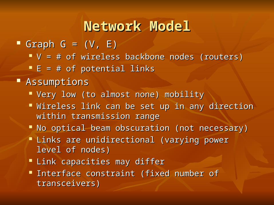
Network ModelNetwork Model Graph G = (V, E)Graph G = (V, E)

V = # of wireless backbone nodes (routers) V = # of wireless backbone nodes (routers) E = # of potential links E = # of potential links

AssumptionsAssumptions Very low (to almost none) mobilityVery low (to almost none) mobility Wireless link can be set up in any direction within Wireless link can be set up in any direction within

transmission rangetransmission range No optical beam obscuration (not necessary)No optical beam obscuration (not necessary) Links are unidirectional (varying power level of nodes)Links are unidirectional (varying power level of nodes) Link capacities may differLink capacities may differ Interface constraint (fixed number of transceivers)Interface constraint (fixed number of transceivers)

Network Model (contd.)Network Model (contd.)

Traffic ProfileTraffic Profile Aggregate traffic demands between sources & Aggregate traffic demands between sources &

destinationsdestinations (x (x y) traffic demand y) traffic demand ≠≠ (y (y x) traffic demand x) traffic demand Collection of individual flows:Collection of individual flows:

Poisson arrival time with rate Poisson arrival time with rate λλi

Exponential holding times with mean TExponential holding times with mean Ti

CBR for each flow with rate RCBR for each flow with rate Ri

Mean aggregate traffic for each ingress-egress pair is Mean aggregate traffic for each ingress-egress pair is λλiTTiRRi

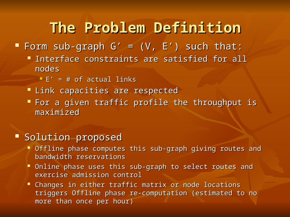
The Problem DefinitionThe Problem Definition Form sub-graph G’ = (V, E’) such that:Form sub-graph G’ = (V, E’) such that:

Interface constraints are satisfied for all nodesInterface constraints are satisfied for all nodes E’ = # of actual linksE’ = # of actual links

Link capacities are respectedLink capacities are respected For a given traffic profile the throughput is maximized For a given traffic profile the throughput is maximized

Solution proposedSolution proposed Offline phase computes this sub-graph giving routes and bandwidth Offline phase computes this sub-graph giving routes and bandwidth

reservationsreservations Online phase uses this sub-graph to select routes and exercise Online phase uses this sub-graph to select routes and exercise

admission controladmission control Changes in either traffic matrix or node locations triggers Offline Changes in either traffic matrix or node locations triggers Offline

phase re-computation (estimated to no more than once per hour)phase re-computation (estimated to no more than once per hour)

Integrated Topology Control and RoutingIntegrated Topology Control and Routing Step 1Step 1

A demand is chosen based on some criteriaA demand is chosen based on some criteria Locally optimal paths (maximum K) are computedLocally optimal paths (maximum K) are computed Fractions of the demand are reserved on each of these paths based on Fractions of the demand are reserved on each of these paths based on

some criteriasome criteria Step 2Step 2

Potential links on paths thus found, are marked as Actual linksPotential links on paths thus found, are marked as Actual links Step 3Step 3

Capacity on each link is decreased to reflect the reserved bandwidthCapacity on each link is decreased to reflect the reserved bandwidth Step 4Step 4

Graph is updated by removing all potential links violating interface Graph is updated by removing all potential links violating interface constraintconstraint

Step 5Step 5 Steps 1, 2, 3 and 4 are repeated till all demands are either met (partially Steps 1, 2, 3 and 4 are repeated till all demands are either met (partially

or fully) or rejectedor fully) or rejected

Ordering of Demand Selection SequenceOrdering of Demand Selection Sequence Bi-directional linksBi-directional links Two interfaces eachTwo interfaces each All demands are sameAll demands are same Traffic MatrixTraffic Matrix

{t{t1212, t, t3434, t, t5656, t, t7878}}

3 5 7

4 6 8

1 2

(a) Virtual Topology(a) Virtual Topology

3 5 7

4 6 8

1 2

(b) t(b) t1212 satisfied satisfied

3 5 7

4 6 8

1 2

(c) t(c) t3434, t, t5656, t, t7878 satisfied satisfied

Offline computationsOffline computations Basic Rollout Algorithm (one step look ahead)Basic Rollout Algorithm (one step look ahead)

Optimal cost approximated by cost of base policyOptimal cost approximated by cost of base policy Example problem: Maximize G(u) whereExample problem: Maximize G(u) where

U is a finite set of feasible solutionsU is a finite set of feasible solutions u u єє U ; u = (u U ; u = (u11, …, u, …, uNN)) ““Base heuristic” extends any partial solution to fullBase heuristic” extends any partial solution to full

(u(u11, …, u, …, unn) (n < N) ) (n < N) (u (u11, …, u, …, uNN))

Let H(uLet H(u11, …, u, …, unn) = G(u) = G(u11, …, u, …, uNN) ) Rollout algo R extends partial solution by one component Rollout algo R extends partial solution by one component

R(uR(u11, …, u, …, un-1n-1) ) (u (u11, …, u, …, unn))

uunn is chosen to maximize H(u is chosen to maximize H(u11, …, u, …, unn) )

Rollout algorithm for TCRRollout algorithm for TCRa) Path Computationa) Path Computation

Step 1Step 1 i=0; // number of paths found for a demandi=0; // number of paths found for a demand d is aggregate demand for one ingress-egress d is aggregate demand for one ingress-egress

pair (dpair (d00=0 )=0 ) Repeat Step 2 tillRepeat Step 2 till

No more path can be foundNo more path can be found Whole demand is metWhole demand is met i = K // the maximum paths allowed for one ingress-i = K // the maximum paths allowed for one ingress-

egress pairegress pair

Rollout algorithm for TCRRollout algorithm for TCRa) Path Computation (contd.)a) Path Computation (contd.)

Step 2Step 2 Find a path using Constrained Shortest Path First (CSPF)Find a path using Constrained Shortest Path First (CSPF) Should accommodate at least (d - dShould accommodate at least (d - dii) / (K - i) bandwidth) / (K - i) bandwidth ConstraintsConstraints

Interface constraintInterface constraint Available bandwidth on linksAvailable bandwidth on links

ddi+1i+1 = Route as much as possible of remaining demand = Route as much as possible of remaining demand

Decrease bandwidth on links of this path by dDecrease bandwidth on links of this path by di+1i+1

i = i + 1i = i + 1

Rollout algorithm for TCR Rollout algorithm for TCR b) Base Heuristicb) Base Heuristic

Routes demands in decreasing order of Routes demands in decreasing order of magnitudemagnitude

Uses the path computation method discussedUses the path computation method discussed Demands are either met (fully or partially) or Demands are either met (fully or partially) or

are blocked (assigned ‘null’ routes)are blocked (assigned ‘null’ routes)

Rollout algorithm for TCR Rollout algorithm for TCR c) Index Rollout Algorithmc) Index Rollout Algorithm

At the nAt the nthth step demands (t step demands (t11,…, t,…, tn-1n-1) have been seen) have been seen

Choose tChoose tnn from amongst the demands remaining to from amongst the demands remaining to

maximize the throughput given by the “base maximize the throughput given by the “base heuristic” on partial solution (theuristic” on partial solution (t11, …, t, …, tnn))

Always performs at least as well as the “base Always performs at least as well as the “base heuristic”heuristic”

Online routing and Admission ControlOnline routing and Admission Control

When a flow arrives at sourceWhen a flow arrives at source Check available reserved BW on all pre-computed paths Check available reserved BW on all pre-computed paths

for that ingress-egress pairfor that ingress-egress pair If not enough BW available on any one path, check If not enough BW available on any one path, check

reserved and also unreserved BW on all pre-computed reserved and also unreserved BW on all pre-computed paths for that pair (leave other pairs alone!!)paths for that pair (leave other pairs alone!!)

If still not enough BW, block flow If still not enough BW, block flow admission control admission control Path selection from amongst pre-computed paths Path selection from amongst pre-computed paths

Minimum BW first: allows larger demands in futureMinimum BW first: allows larger demands in future Maximum BW first: ensures fairness amongst routesMaximum BW first: ensures fairness amongst routes

Computational ComplexityComputational Complexity Online algorithmOnline algorithm

O(K) for routing decision for at most K paths O(K) for routing decision for at most K paths ~ O(1) since K is fixed~ O(1) since K is fixed

Offline algorithmOffline algorithm N = # of nodes; M = # of traffic demands; N = # of nodes; M = # of traffic demands; Shortest path = O(NShortest path = O(N22) // modified Dijkstra’s) // modified Dijkstra’s Sorting demands = O(MlogM) << O(NSorting demands = O(MlogM) << O(N22) // ignored) // ignored Base Heuristic = O(KMNBase Heuristic = O(KMN22) )

Max of K paths for each of M demandsMax of K paths for each of M demands Index rollout = O(KMIndex rollout = O(KM33NN22))

Each decision step, for each M demand “base heuristic” is usedEach decision step, for each M demand “base heuristic” is used M decision steps in allM decision steps in all

Simulation ParametersSimulation Parameters

50 nodes uniformly distributed (avg. 7.5 neighbors)50 nodes uniformly distributed (avg. 7.5 neighbors) Transmission ranges for all nodes are sameTransmission ranges for all nodes are same Capacity of each link = 100 units in each directionCapacity of each link = 100 units in each direction # of nodes capable of being source/destination = 12# of nodes capable of being source/destination = 12 # of source-destination pairs = 100# of source-destination pairs = 100 Arrival Poisson rate (Arrival Poisson rate (λλi): uniform between 10 and 20 per unit time): uniform between 10 and 20 per unit time

Mean Holding time (TMean Holding time (Tii): uniform between 1 and 2 units of time): uniform between 1 and 2 units of time # of transmitters = # of receivers = 3# of transmitters = # of receivers = 3 Max # of paths per ingress-egress pair (K) = 3Max # of paths per ingress-egress pair (K) = 3 Weight of each link for CSPF = 1 // shortest path = min-hop pathWeight of each link for CSPF = 1 // shortest path = min-hop path Simulation was run 10 times for 30 units of time each, starting each time Simulation was run 10 times for 30 units of time each, starting each time

with above parameterswith above parameters

Simulation results ISimulation results I

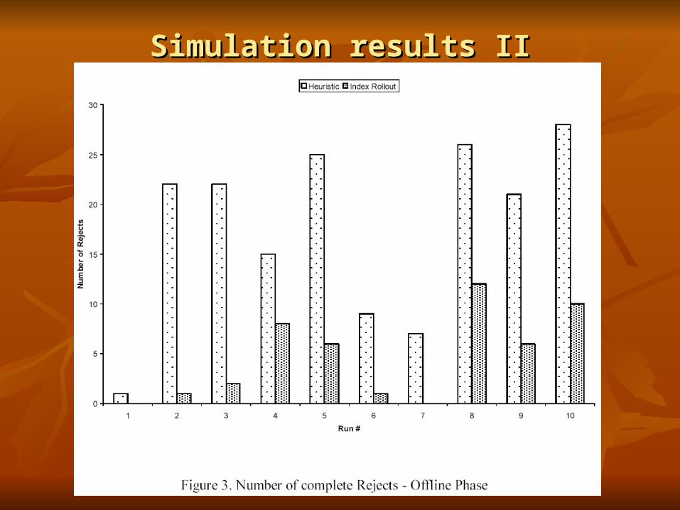
Simulation results IISimulation results II

Simulation results IIISimulation results III

ConclusionConclusion

Index rollout works better than “base heuristic”Index rollout works better than “base heuristic” 10.83% increase in throughput10.83% increase in throughput 73.86% decrease in flow rejects73.86% decrease in flow rejects

On passing same traffic parameters to both Offline On passing same traffic parameters to both Offline and Online phase, rollout admits 12.61% more calls and Online phase, rollout admits 12.61% more calls than the “base heuristic”than the “base heuristic”

On fixing K and also M, we get O(NOn fixing K and also M, we get O(N22) time ) time complexitycomplexity