Professor John W. Norbury - Fisica · GENERAL RELATIVITY & COSMOLOGY for Undergraduates Professor...

GENERAL RELATIVITY &

COSMOLOGY

for Undergraduates

Professor John W. Norbury

Physics DepartmentUniversity of Wisconsin-Milwaukee

P.O. Box 413Milwaukee, WI 53201

1997

Contents

1 NEWTONIAN COSMOLOGY 51.1 Introduction . . . . . . . . . . . . . . . . . . . . . . . . . . . . 51.2 Equation of State . . . . . . . . . . . . . . . . . . . . . . . . . 5

1.2.1 Matter . . . . . . . . . . . . . . . . . . . . . . . . . . . 61.2.2 Radiation . . . . . . . . . . . . . . . . . . . . . . . . . 6

1.3 Velocity and Acceleration Equations . . . . . . . . . . . . . . 71.4 Cosmological Constant . . . . . . . . . . . . . . . . . . . . . . 9

1.4.1 Einstein Static Universe . . . . . . . . . . . . . . . . . 11

2 APPLICATIONS 132.1 Conservation laws . . . . . . . . . . . . . . . . . . . . . . . . 132.2 Age of the Universe . . . . . . . . . . . . . . . . . . . . . . . 142.3 Inflation . . . . . . . . . . . . . . . . . . . . . . . . . . . . . . 152.4 Quantum Cosmology . . . . . . . . . . . . . . . . . . . . . . . 16

2.4.1 Derivation of the Schrodinger equation . . . . . . . . . 162.4.2 Wheeler-DeWitt equation . . . . . . . . . . . . . . . . 17

2.5 Summary . . . . . . . . . . . . . . . . . . . . . . . . . . . . . 182.6 Problems . . . . . . . . . . . . . . . . . . . . . . . . . . . . . 192.7 Answers . . . . . . . . . . . . . . . . . . . . . . . . . . . . . . 202.8 Solutions . . . . . . . . . . . . . . . . . . . . . . . . . . . . . 21

3 TENSORS 233.1 Contravariant and Covariant Vectors . . . . . . . . . . . . . . 233.2 Higher Rank Tensors . . . . . . . . . . . . . . . . . . . . . . . 263.3 Review of Cartesian Tensors . . . . . . . . . . . . . . . . . . . 273.4 Metric Tensor . . . . . . . . . . . . . . . . . . . . . . . . . . . 28

3.4.1 Special Relativity . . . . . . . . . . . . . . . . . . . . . 303.5 Christoffel Symbols . . . . . . . . . . . . . . . . . . . . . . . . 31

1

2 CONTENTS

3.6 Christoffel Symbols and Metric Tensor . . . . . . . . . . . . . 363.7 Riemann Curvature Tensor . . . . . . . . . . . . . . . . . . . 383.8 Summary . . . . . . . . . . . . . . . . . . . . . . . . . . . . . 393.9 Problems . . . . . . . . . . . . . . . . . . . . . . . . . . . . . 403.10 Answers . . . . . . . . . . . . . . . . . . . . . . . . . . . . . . 413.11 Solutions . . . . . . . . . . . . . . . . . . . . . . . . . . . . . 42

4 ENERGY-MOMENTUM TENSOR 454.1 Euler-Lagrange and Hamilton’s Equations . . . . . . . . . . . 454.2 Classical Field Theory . . . . . . . . . . . . . . . . . . . . . . 47

4.2.1 Classical Klein-Gordon Field . . . . . . . . . . . . . . 484.3 Principle of Least Action . . . . . . . . . . . . . . . . . . . . 494.4 Energy-Momentum Tensor for Perfect Fluid . . . . . . . . . . 494.5 Continuity Equation . . . . . . . . . . . . . . . . . . . . . . . 514.6 Interacting Scalar Field . . . . . . . . . . . . . . . . . . . . . 514.7 Cosmology with the Scalar Field . . . . . . . . . . . . . . . . 53

4.7.1 Alternative derivation . . . . . . . . . . . . . . . . . . 554.7.2 Limiting solutions . . . . . . . . . . . . . . . . . . . . 564.7.3 Exactly Solvable Model of Inflation . . . . . . . . . . . 594.7.4 Variable Cosmological Constant . . . . . . . . . . . . . 614.7.5 Cosmological constant and Scalar Fields . . . . . . . . 634.7.6 Clarification . . . . . . . . . . . . . . . . . . . . . . . . 644.7.7 Generic Inflation and Slow-Roll Approximation . . . . 654.7.8 Chaotic Inflation in Slow-Roll Approximation . . . . . 674.7.9 Density Fluctuations . . . . . . . . . . . . . . . . . . . 724.7.10 Equation of State for Variable Cosmological Constant 734.7.11 Quantization . . . . . . . . . . . . . . . . . . . . . . . 77

4.8 Problems . . . . . . . . . . . . . . . . . . . . . . . . . . . . . 80

5 EINSTEIN FIELD EQUATIONS 835.1 Preview of Riemannian Geometry . . . . . . . . . . . . . . . . 84

5.1.1 Polar Coordinate . . . . . . . . . . . . . . . . . . . . . 845.1.2 Volumes and Change of Coordinates . . . . . . . . . . 855.1.3 Differential Geometry . . . . . . . . . . . . . . . . . . 885.1.4 1-dimesional Curve . . . . . . . . . . . . . . . . . . . . 895.1.5 2-dimensional Surface . . . . . . . . . . . . . . . . . . 925.1.6 3-dimensional Hypersurface . . . . . . . . . . . . . . . 96

5.2 Friedmann-Robertson-Walker Metric . . . . . . . . . . . . . . 995.2.1 Christoffel Symbols . . . . . . . . . . . . . . . . . . . . 101

CONTENTS 3

5.2.2 Ricci Tensor . . . . . . . . . . . . . . . . . . . . . . . . 1025.2.3 Riemann Scalar and Einstein Tensor . . . . . . . . . . 1035.2.4 Energy-Momentum Tensor . . . . . . . . . . . . . . . 1045.2.5 Friedmann Equations . . . . . . . . . . . . . . . . . . 104

5.3 Problems . . . . . . . . . . . . . . . . . . . . . . . . . . . . . 105

6 Einstein Field Equations 107

7 Weak Field Limit 109

8 Lagrangian Methods 111

4 CONTENTS

Chapter 1

NEWTONIANCOSMOLOGY

1.1 Introduction

Many of the modern ideas in cosmology can be explained without the needto discuss General Relativity. The present chapter represents an attempt todo this based entirely on Newtonian mechanics. The equations describingthe velocity (called the Friedmann equation) and acceleration of the universeare derived from Newtonian mechanics and also the cosmological constantis introduced within a Newtonian framework. The equations of state arealso derived in a very simple way. Applications such as conservation laws,the age of the universe and the inflation, radiation and matter dominatedepochs are discussed.

1.2 Equation of State

In what follows the equation of state for non-relativistic matter and radiationwill be needed. In particular an expression for the rate of change of density,ρ, will be needed in terms of the density ρ and pressure p. (The definitionx ≡ dx

dt , where t is time, is being used.) The first law of thermodynamics is

dU + dW = dQ (1.1)

where U is the internal energy, W is the work and Q is the heat transfer.Ignoring any heat transfer and writing dW = Fdr = pdV where F is the

5

6 CHAPTER 1. NEWTONIAN COSMOLOGY

force, r is the distance, p is the pressure and V is the volume, then

dU = −pdV. (1.2)

Assuming that ρ is a relativistic energy density means that the energy isexpressed as

U = ρV (1.3)

from which it follows that

U = ρV + ρV = −pV (1.4)

where the term on the far right hand side results from equation (1.2). WritingV ∝ r3 implies that V

V = 3 rr . Thus

ρ = −3(ρ+ p)r

r(1.5)

1.2.1 Matter

Writing the density of matter as

ρ =M

43πr

3(1.6)

it follows thatρ ≡ dρ

drr = −3ρ

r

r(1.7)

so that by comparing to equation (1.5), it follows that the equation of statefor matter is

p = 0. (1.8)

This is the same as obtained from the ideal gas law for zero temperature.Recall that in this derivation we have not introduced any kinetic energy, sowe are talking about zero temperature.

1.2.2 Radiation

The equation of state for radiation can be derived by considering radiationmodes in a cavity based on analogy with a violin string [12]. For a standingwave on a string fixed at both ends

L =nλ

2(1.9)

1.3. VELOCITY AND ACCELERATION EQUATIONS 7

where L is the length of the string, λ is the wavelength and n is a positiveinteger (n = 1, 2, 3.....). Radiation travels at the velocity of light, so that

c = fλ = f2Ln

(1.10)

where f is the frequency. Thus substituting f = n2Lc into Planck’s formula

U = hω = hf , where h is Planck’s constant, gives

U =nhc

21L∝ V −1/3. (1.11)

Using equation (1.2) the pressure becomes

p ≡ −dUdV

=13U

V. (1.12)

Using ρ = U/V , the radiation equation of state is

p =13ρ. (1.13)

It is customary to combine the equations of state into the form

p =γ

3ρ (1.14)

where γ ≡ 1 for radiation and γ ≡ 0 for matter. These equations of stateare needed in order to discuss the radiation and matter dominated epochswhich occur in the evolution of the Universe.

1.3 Velocity and Acceleration Equations

The Friedmann equation, which specifies the speed of recession, is obtainedby writing the total energy E as the sum of kinetic plus potential energyterms (and using M = 4

3πr3ρ )

E = T + V =12mr2 −GMm

r=

12mr2(H2 − 8πG

3ρ) (1.15)

where the Hubble constant H ≡ rr , m is the mass of a test particle in the

potential energy field enclosed by a gas of dust of mass M , r is the distancefrom the center of the dust to the test particle and G is Newton’s constant.


Recall that the escape velocity is just vescape =√

2GMr =

√8πG

3 ρr2, so thatthe above equation can also be written

r2 = v2escape − k′13− 2 (1.16)

with k′ ≡ −2Em . The constant k′ can either be negative, zero or positive

corresponding to the total energy E being positive, zero or negative. Fora particle in motion near the Earth this would correspond to the particleescaping (unbound), orbiting (critical case) or returning (bound) to Earthbecause the speed r would be greater, equal to or smaller than the escapespeed vescape. Later this will be analagous to an open, flat or closed universe.Equation (1.15) is re-arranged as

H2 =8πG

3ρ+

2Emr2

.13− 3 (1.17)

Defining k ≡ − 2Ems2

and writing the distance in terms of the scale factor R

and a constant length s as r(t) ≡ R(t)s, it follows that rr = R

R and rr = R

R ,giving the Friedmann equation

H2 ≡ (R

R)2 =

8πG3

ρ− k

R2(1.18)

which specifies the speed of recession. The scale factor is introduced becausein General Relativity it is space itself which expands [19]. Even though thisequation is derived for matter, it is also true for radiation. (In fact it is alsotrue for vacuum, with Λ ≡ 8πGρvac, where Λ is the cosmological constantand ρvac is the vacuum energy density which just replaces the ordinary den-sity. This is discussed later.) Exactly the same equation is obtained fromthe general relativistic Einstein field equations [13]. According to Guth [10],k can be rescaled so that instead of being negative, zero or positive it takeson the values −1, 0 or +1. From a Newtonian point of view this correspondsto unbound, critical or bound trajectories as mentioned above. From a geo-metric, general relativistic point of view this corresponds to an open, flat orclosed universe.

In elementary mechanics the speed v of a ball dropped from a height ris evaluated from the conservation of energy equation as v =

√2gr, where

g is the acceleration due to gravity. The derivation shown above is exactlyanalagous to such a calculation. Similarly the acceleration a of the ball iscalculated as a = g from Newton’s equation F = mr, where F is the force

1.4. COSMOLOGICAL CONSTANT 9

and the acceleration is r ≡ d2rdt2

. The acceleration for the universe is obtainedfrom Newton’s equation

−GMm

r2= mr.13− 5 (1.19)

Again using M = 43πr

3ρ and rr = R

R gives the acceleration equation

F

mr≡ r

r≡ R

R= −4πG

3ρ. (1.20)

However because M = 43πr

3ρ was used, it is clear that this accelerationequation holds only for matter. In our example of the falling ball instead ofthe acceleration being obtained from Newton’s Law, it can also be obtainedby taking the time derivative of the energy equation to give a = dv

dt = v dvdr =(√

2gr)(√

2g 12√r) = g. Similarly, for the general case one can take the time

derivative of equation (1.18) (valid for matter and radiation)

d

dtR2 = 2RR =

8πG3

d

dt(ρR2). (1.21)

Upon using equation (1.5) the acceleration equation is obtained as

R

R= −4πG

3(ρ+ 3p) = −4πG

3(1 + γ)ρ (1.22)

which reduces to equation (1.20) for the matter equation of state (γ = 0).Exactly the same equation is obtained from the Einstein field equations [13].

1.4 Cosmological Constant

In both Newtonian and relativistic cosmology the universe is unstable togravitational collapse. Both Newton and Einstein believed that the Universeis static. In order to obtain this Einstein introduced a repulsive gravitationalforce, called the cosmological constant, and Newton could have done exactlythe same thing, had he believed the universe to be finite.

In order to obtain a possibly zero acceleration, a positive term (conven-tionally taken as Λ

3 ) is added to the acceleration equation (1.22) as

R

R= −4πG

3(ρ+ 3p) +

Λ3

(1.23)


which, with the proper choice of Λ can give the required zero accelerationfor a static universe. Again exactly the same equation is obtained from theEinstein field equations [13]. What has been done here is entirely equivalentto just adding a repulsive gravitational force in Newton’s Law. The questionnow is how this repulsive force enters the energy equation (1.18). Identifyingthe force from

r

r=R

R≡ Frepulsive

mr≡ Λ

3(1.24)

and using

Frepulsive =Λ3mr ≡ −dV

dr(1.25)

gives the potential energy as

Vrepulsive = −12

Λ3mr2 (1.26)

which is just a repulsive simple harmonic oscillator. Substituting this intothe conservation of energy equation

E = T + V =12mr2 −GMm

r− 1

2Λ3mr2 =

12mr2(H2 − 8πG

3ρ− Λ

3) (1.27)

gives

H2 ≡ (R

R)2 =

8πG3

ρ− k

R2+

Λ3. (1.28)

Equations (1.28) and (1.23) constitute the fundamental equations of motionthat are used in all discussions of Friedmann models of the Universe. Exactlythe same equations are obtained from the Einstein field equations [13].

Let us comment on the repulsive harmonic oscillator obtained above.Recall one of the standard problems often assigned in mechanics courses.The problem is to imagine that a hole has been drilled from one side of theEarth, through the center and to the other side. One is to show that if aball is dropped into the hole, it will execute harmonic motion. The solutionis obtained by noting that whereas gravity is an inverse square law for pointmasses M and m separated by a distance r as given by F = GMm

r2 , yet if oneof the masses is a continous mass distribution represented by a density thenF = G4

3πρmr. The force rises linearly as the distance is increased becausethe amount of matter enclosed keeps increasing. Thus the gravitational forcefor a continuous mass distribution rises like Hooke’s law and thus oscillatorysolutions are encountered. This sheds light on our repulsive oscillator found

1.4. COSMOLOGICAL CONSTANT 11

above. In this case we want the gravity to be repulsive, but the cosmologicalconstant acts just like the uniform matter distribution.

Finally authors often write the cosmological constant in terms of a vac-uum energy density as Λ ≡ 8πGρvac so that the velocity and accelerationequations become

H2 ≡ (R

R)2 =

8πG3

ρ− k

R2+

Λ3

=8πG

3(ρ+ ρvac)−

k

R2(1.29)

and

R

R= −4πG

3(1 + γ)ρ+

Λ3

= −4πG3

(1 + γ)ρ+8πG

3ρvac. (1.30)

1.4.1 Einstein Static Universe

Although we have noted that the cosmological constant provides repulsion,it is interesting to calculate its exact value for a static universe [14, 15]. TheEinstein static universe requires R = R0 = constant and thus R = R = 0.The case R = 0 will be examined first. From equation (1.23) this requiresthat

Λ = 4πG(ρ+ 3p) = 4πG(1 + γ)ρ. (1.31)

If there is no cosmological constant (Λ = 0) then either ρ = 0 which is anempty universe, or p = −1

3ρ which requires negative pressure. Both of thesealternatives were unacceptable to Einstein and therefore he concluded thata cosmological constant was present, i.e. Λ 6= 0. From equation (1.31) thisimplies

ρ =Λ

4πG(1 + γ)(1.32)

and because ρ is positive this requires a positive Λ. Substituting equa-tion (1.32) into equation (1.28) it follows that

Λ =3(1 + γ)

3 + γ[(R

R0)2 +

k

R20

]. (1.33)

Now imposing R = 0 and assuming a matter equation of state (γ = 0)implies Λ = k

R20. However the requirement that Λ be positive forces k = +1

giving

Λ =1R2

0

= constant. (1.34)


Thus the cosmological constant is not any old value but rather simply theinverse of the scale factor squared, where the scale factor has a fixed valuein this static model.

Chapter 2

APPLICATIONS

2.1 Conservation laws

Just as the Maxwell equations imply the conservation of charge, so too doour velocity and acceleration equations imply conservation of energy. Theenergy-momentum conservation equation is derived by setting the covariantderivative of the energy momentum tensor equal to zero. The same result isachieved by taking the time derivative of equation (1.29). The result is

ρ+ 3(ρ+ p)R

R= 0. (2.1)

This is identical to equation (1.5) illustrating the intersting connection be-tweeen thermodynamics and General Relativity that has been discussed re-cently [16]. The point is that we used thermodynamics to derive our velocityand acceleration equations and it is no surprise that the thermodynamic for-mula drops out again at the end. However, the velocity and accelerationequations can be obtained directly from the Einstein field equations. Thusthe Einstein equations imply this thermodynamic relationship in the aboveequation.

The above equation can also be written as

d

dt(ρR3) + p

dR3

dt= 0 (2.2)

and from equation (1.14), 3(ρ+ p) = (3 + γ)ρ, it follows that

d

dt(ρR3+γ) = 0. (2.3)

13

14 CHAPTER 2. APPLICATIONS

Integrating this we obtainρ =

c

R3+γ(2.4)

where c is a constant. This shows that the density falls as 1R3 for matter and

1R4 for radiation as expected.

Later we shall use these equations in a different form as follows. Fromequation (2.1),

ρ′ + 3(ρ+ p)1R

= 0 (2.5)

where primes denote derivatives with respect to R, i.e. x′ ≡ dx/dR. Alter-natively

d

dR(ρR3) + 3pR2 = 0 (2.6)

so that1

R3+γ

d

dR(ρR3+γ) = 0 (2.7)

which is consistent with equation (2.4)

2.2 Age of the Universe

Recent measurements made with the Hubble space telescope [17] have de-termined that the age of the universe is younger than globular clusters. Apossible resolution to this paradox involves the cosmological constant [18].We illustrate this as follows.

Writing equation (1.28) as

R2 =8πG

3(ρ+ ρvac)R2 − k (2.8)

the present day value of k is

k =8πG

3(ρ0 + ρ0vac)R2

0 −H20R

20 (2.9)

with H2 ≡ ( RR)2. Present day values of quantities have been denoted with asubscript 0. Substituting equation (2.9) into equation (2.8) yields

R2 =8πG

3(ρR2 − ρ0R

20 + ρvacR

2 − ρ0vacR20)−H2

0R20. (2.10)

2.3. INFLATION 15

Integrating gives the expansion age

T0 =∫ R0

0

dR

R=∫ R0

0

dR√8πG

3 (ρR2 − ρ0R20 + ρvacR2 − ρ0vacR2

0)−H20R

20

.

(2.11)For the cosmological constant ρvac = ρ0vac and because R2 < R2

0 then anon zero cosmological constant will give an age larger than would have beenobtained were it not present. Our aim here is simply to show that theinclusion of a cosmological constant gives an age which is larger than if noconstant were present.

2.3 Inflation

In this section only a flat k = 0 universe will be discussed. Results foran open or closed universe can easily be obtained and are discussed in thereferences [13].

Currently the universe is in a matter dominated phase whereby the dom-inant contribution to the energy density is due to matter. However the earlyuniverse was radiation dominated and the very early universe was vacuumdominated. Setting k = 0, there will only be one term on the right handside of equation (1.29) depending on what is dominating the universe. For amatter (γ = 0) or radiation (γ = 1) dominated universe the right hand sidewill be of the form 1

R3+γ (ignoring vacuum energy), whereas for a vacuumdominated universe the right hand side will be a constant. The solutionto the Friedmann equation for a radiation dominated universe will thus beR ∝ t 1

2 , while for the matter dominated case it will be R ∝ t 23 . One can see

that these results give negative acceleration, corresponding to a deceleratingexpanding universe.

Inflation [19] occurs when the vacuum energy contribution dominates theordinary density and curvature terms in equation (1.29). Assuming theseare negligible and substituting Λ = constant, results in R ∝ exp(t). Theacceleration is positive, corresponding to an accelerating expanding universecalled an inflationary universe.


2.4 Quantum Cosmology

2.4.1 Derivation of the Schrodinger equation

The Wheeler-DeWitt equation will be derived in analogy with the 1 dimen-sional Schrodinger equation, which we derive herein for completeness. TheLagrangian L for a single particle moving in a potential V is

L = T − V (2.12)

where T = 12mx

2 is the kinetic energy, V is the potential energy. The actionis S =

∫Ldt and varying the action according to δS = 0 results in the

Euler-Lagrange equation (equation of motion)

d

dt(∂L

∂x)− ∂L

∂x= 0 (2.13)

or just

P =∂L

∂x(2.14)

whereP ≡ ∂L

∂x. (2.15)

(Note P is the momentum but p is the pressure.) The Hamiltonian H isdefined as

H(P, x) ≡ Px− L(x, x). (2.16)

For many situations of physical interest, such as a single particle moving ina harmonic oscillator potential V = 1

2kx2, the Hamiltonian becomes

H = T + V =P 2

2m+ V = E (2.17)

where E is the total energy. Quantization is achieved by the operator re-placements P → P = −i ∂∂x and E → E = i ∂∂t where we are leaving offfactors of h and we are considering the 1-dimensional equation only. TheSchrodinger equation is obtained by writing the Hamiltonian as an operatorH acting on a wave function Ψ as in

HΨ = EΨ (2.18)

and making the above operator replacements to obtain

(− 12m

∂2

∂x2+ V )Ψ = i

∂

∂tΨ (2.19)

which is the usual form of the 1-dimensional Schrodinger equation writtenin configuration space.

2.4. QUANTUM COSMOLOGY 17

2.4.2 Wheeler-DeWitt equation

The discussion of the Wheeler-DeWitt equation in the minisuperspace ap-proximation [20, 21, 11, 22] is usually restricted to closed (k = +1) andempty (ρ = 0) universes. Atkatz [11] presented a very nice discussion forclosed and empty universes. Herein we consider closed, open and flat andnon-empty universes. It is important to consider the possible presence ofmatter and radiation as they might otherwise change the conclusions. Thuspresented below is a derivation of the Wheeler-DeWitt equation in the min-isuperspace approximation which also includes matter and radiation andarbitrary values of k.

The Lagrangian is

L = −κR3[(R

R)2 − k

R2+

8πG3

(ρ+ ρvac)] (2.20)

with κ ≡ 3π4G . The momentum conjugate to R is

P ≡ ∂L

∂R= −κ2RR. (2.21)

Substituting L and P into the Euler-Lagrange equation, P − ∂L∂R = 0, equa-

tion (1.29) is recovered. (Note the calculation of ∂L∂R is simplified by using

the conservation equation (2.5) with equation (1.14), namely ρ′ + ρ′vac =−(3 + γ)ρ/R). The Hamiltonian H ≡ PR− L is

H(R, R) = −κR3[(R

R)2 +

k

R2− 8πG

3(ρ+ ρvac)] ≡ 0 (2.22)

which has been written in terms of R to show explicitly that the Hamiltonianis identically zero and is not equal to the total energy as before. (Compareequation (1.29)). In terms of the conjugate momentum

H(P,R) = −κR3[P 2

4κ2R4+

k

R2− 8πG

3(ρ+ ρvac)] = 0 (2.23)

which, of course is also equal to zero. Making the replacement P → −i ∂∂Rand imposing HΨ = 0 results in the Wheeler-DeWitt equation in the min-isuperspace approximation for arbitrary k and with matter or radiation (ρterm) included gives

{− ∂2

∂R2+

9π2

4G2[(kR2 − 8πG

3(ρ+ ρvac)R4]}Ψ = 0. (2.24)


Using equation (2.4) the Wheeler-DeWitt equation becomes

{− ∂2

∂R2+

9π2

4G2[kR2 − Λ

3R4 − 8πG

3cR1−γ ]}Ψ = 0. (2.25)

This just looks like the zero energy Schrodinger equation [21] with a potentialgiven by

V (R) = kR2 − Λ3R4 − 8πG

3cR1−γ . (2.26)

For the empty Universe case of no matter or radiation (c = 0) the po-tential V (R) is plotted in Figure 1 for the cases k = +1, 0,−1 respectivelycorresponding to closed [21], open and flat universes. It can be seen that onlythe closed universe case provides a potential barrier through which tunnel-ing can occur. This provides a clear illustration of the idea that only closeduniverses can arise through quantum tunneling [22]. If radiation (γ = 1 andc 6= 0) is included then only a negative constant will be added to the poten-tial (because the term R1−γ will be constant for γ = 1) and these conclusionsabout tunneling will not change. The shapes in Figure 1 will be identicalexcept that the whole graph will be shifted downwards by a constant withthe inclusion of radiation. (For matter (γ = 0 and c 6= 0) a term growinglike R will be included in the potential which will only be important for verysmall R and so the conclusions again will not be changed.) To summarize,only closed universes can arise from quantum tunneling even if matter orradiation are present.

2.5 Summary

2.6. PROBLEMS 19

2.6 Problems

2.1


2.7 Answers

2.1

2.8. SOLUTIONS 21

2.8 Solutions

2.1

2.2

Chapter 3

TENSORS

3.1 Contravariant and Covariant Vectors

Let us imagine that an ’ordinary’ 2-dimensional vector has components (x, y)or (x1, x2) (read as x superscript 2 not x squared) in a certain coordinatesystem and components (x, y) or (x1, x2) when that coordinate system is ro-tated by angle θ (but with the vector remaining fixed). Then the componentsare related by [1] (

xy

)=

(cos θ sin θsin θ cos θ

)(xy

)(3.1)

Notice that we are using superscipts (xi) for the components of our or-dinary vectors (instead of the usual subscripts used in freshman physics),which henceforth we are going to name contravariant vectors. We empha-size that these are just the ordinary vectors one comes across in freshmanphysics.

Expanding the matrix equation we have

x = x cos θ + y sin θ (3.2)y = −x sin θ + y cos θ

from which it follows that

∂x

∂x= cos θ

∂x

∂y= sin θ (3.3)

23

24 CHAPTER 3. TENSORS

∂y

∂x= − sin θ

∂y

∂y= cos θ

so that

x =∂x

∂xx+

∂x

∂yy (3.4)

y =∂y

∂xx+

∂y

∂yy

which can be written compactly as

xi =∂xi

∂xjxj (3.5)

where we will always be using the Einstein summation convention for doublyrepeated indices. (i.e. xiyi ≡

∑i xiyi)

Instead of defining an ordinary (contravariant) vector as a little arrowpointing in some direction, we shall instead define it as an object whose com-ponents transform according to equation(3.5). This is just a fancy versionof equation(3.1), which is another way to define a vector as what happensto the components upon rotation (instead of the definition of a vector as alittle arrow). Notice that we could have written down a diferential versionof (3.5) just from what we know about calculus. Using the infinitessimal dxi

(instead of xi) it follows immediately that

dxi =∂xi

∂xjdxj (3.6)

which is identical to (3.5) and therefore we must say that dxi forms anordinary or contravariant vector (or an infinitessimally tiny arrow).

While we are on the subject of calculus and infinitessimals let’s thinkabout ∂

∂xiwhich is kind of like the ’inverse’ of dxi. From calculus if f =

f(x, y) and x = x(x, y) and y = y(x, y) (which is what (3.3) is saying) then

∂f

∂x=∂f

∂x

∂x

∂x+∂f

∂y

∂y

∂x(3.7)

∂f

∂y=∂f

∂x

∂x

∂y+∂f

∂y

∂y

∂y

or simply∂f

∂xi=

∂f

∂xj∂xj

∂xi. (3.8)

3.1. CONTRAVARIANT AND COVARIANT VECTORS 25

Let’s ’remove’ f and just write

∂

∂xi=∂xj

∂xi∂

∂xj. (3.9)

which we see is similar to (3.5), and so we might expect that ∂/∂xi arethe ’components’ of a ’non-ordinary’ vector. Notice that the index is in thedenominator, so instead of writing ∂/∂xi let’s just always write it as xi forshorthand. Or equivalently define

xi ≡∂

∂xi(3.10)

Thus

xi =∂xj

∂xixj . (3.11)

So now let’s define a contravariant vector Aµ as anything whose componentstransform as (compare (3.5))

Aµ ≡ ∂xµ

∂xνAν

(3.12)

and a covariant vector Aµ (often also called a one-form, or dual vector orcovector)

Aµ = ∂xν

∂xµAν

(3.13)

In calculus we have two fundamental objects dxi and the dual vector ∂/∂xi.If we try to form the dual dual vector ∂/∂(∂/∂xi) we get back dxi [2]. Aset of points in a smooth space is called a manifold and where dxi forms aspace, ∂/∂xi forms the corresponding ’dual’ space [2]. The dual of the dualspace is just the original space dxi. Contravariant and covariant vectors arethe dual of each other. Other examples of dual spaces are row and column

matrices (x y) and

(xy

)and the kets < a| and bras |a > used in quantum

mechanics [3].Before proceeding let’s emphasize again that our definitions of contravari-

ant and covariant vectors in (3.13) and (3.13) are nothing more than fancyversions of (3.1).


3.2 Higher Rank Tensors

Notice that our vector components Aµ have one index, whereas a scalar(e.g. t = time or T = temperature) has zero indices. Thus scalars are calledtensors of rank zero and vectors are called tensors of rank one. We arefamiliar with matrices which have two indices Aij . A contravariant tensor ofrank two is of the form Aµν , rank three Aµνγ etc. A mixed tensor, e.g. Aµν ,is partly covariant and partly contravariant.

In order for an object to be called a tensor it must satisfy the tensortransformation rules, examples of which are (3.13) and (3.13) and

Tµν = ∂xµ

∂xα∂xν

∂xβTαβ .

(3.14)

Tµν =

∂xµ

∂xα∂xβ

∂xνTαβ . (3.15)

Tµνρ =

∂xµ

∂xα∂xν

∂xβ∂xγ

∂xρTαβγ . (3.16)

Thus even though a matrix has two indices Aij , it may not necessarily bea second rank tensor unless it satisfies the above tensor tranformation rulesas well. However all second rank tensors can be written as matrices.

Higher rank tensors can be constructed from lower rank ones by formingwhat is called the outer product or tensor product [14] as follows. For instance

Tαβ ≡ AαBβ (3.17)

orTαβγδ ≡ AαγB

βδ . (3.18)

The tensor product is often written simply as

T = A⊗B (3.19)

(do Problem 3.1) (NNN Next time discuss wedge product - easy - justintroduce antisymmetry).

We can also construct lower rank tensors from higher rank ones by aprocess called contraction, which sets a covariant and contravariant indexequal, and because of the Einstein summation convention equal or repeated

3.3. REVIEW OF CARTESIAN TENSORS 27

indices are summed over. Thus contraction represents setting two indicesequal and summing. For example

Tαβγβ ≡ Tαγ (3.20)

Thus contraction over a pair of indices reduces the rank of a tensor by two[14].

The inner product [14] of two tensors is defined by forming the outerproduct and then contracting over a pair of indices as

Tαβ ≡ AαγBγβ . (3.21)

Clearly the inner product of two vectors (rank one tensors) produces a scalar(rank zero tensor) as

AµBµ = constant ≡ A.B (3.22)

and it can be shown that A.B as defined here is a scalar (do Problem 3.2).A scalar is a tensor of rank zero with the very special transformation law ofinvariance

c = c. (3.23)

It is easily shown, for example, that AµBµ is no good as a definition of innerproduct for vectors because it is not invariant under transformations andtherefore is not a scalar.

3.3 Review of Cartesian Tensors

Let us review the scalar product that we used in freshman physics. We wrotevectors as A = Aiei and defined the scalar product as

A.B ≡ AB cos θ (3.24)

where A and B are the magnitudes of the vectors A and B and θ is theangle between them. Thus

A.B = Aiei.Bj ej

= (ei.ej)AiBj≡ gijAiBj (3.25)


where the metric tensor gij is defined as the dot product of the basis vectors.A Cartesian basis is defined as one in which gij ≡ δij (obtained from

ei.ej = |ei||ej | cos θ = cos θ = δij). That is, the basis vectors are of unitlength and perpendicular to each other in which case

A.B = AiBi

= AxBx +AyBy + .... (3.26)

where the sum (+...) extends to however many dimensions are being consid-ered and

A.A ≡ A2 = AiAi (3.27)

which is just Pythagoras’ theorem, A.A ≡ A2 = AiAi = A2x +A2

y + .......Notice that the usual results we learned about in freshman physics, equa-

tions (3.26) and (3.27), result entirely from requiring gij = δij =

(1 00 1

)in matrix notation.

We could easily have defined a non-Cartesian space, for example, gij =(1 10 1

)in which case Pythagoras’ theorem would change to

A.A ≡ A2 = AiAi = A2x +A2

y +AxAy. (3.28)

Thus it is the metric tensor gij ≡ ei.ej given by the scalar product of theunit vectors which (almost) completely defines the vector space that we areconsidering. Now let’s return to vectors and one-forms (i.e. contravariantand covariant vectors).

3.4 Metric Tensor

We have already seen (in Problem 3.2) that the inner product defined byA.B ≡ AµB

µ transforms as a scalar. (The choice AµBµ won’t do becauseit is not a scalar). However based on the previous section, we would expectthat A.B can also be written in terms of a metric tensor. The most naturalway to do this is

A.B ≡ AµBµ

= gµνAνBµ (3.29)

assuming gµν is a tensor.

3.4. METRIC TENSOR 29

In fact defining A.B ≡ AµBµ ≡ gµνAνBµ makes perfect sense because italso transforms as a scalar (i.e. is invariant). (do Problem 3.3) Thus eitherof the two right hand sides of (3.29) will do equally well as the definition ofthe scalar product, and thus we deduce that

Aµ = gµνAν

(3.30)

so that the metric tensor has the effect of lowering indices. Similarly it canraise indices

Aµ = gµνAν

(3.31)

How is vector A written in terms of basis vectors ? Based on our expe-rience with Cartesian vectors let’s define our basis vectors such that

A.B ≡ AµBµ

= gµνAνBµ

≡ (eµ.eν)AνBµ (3.32)

which imples that vectors can be written in terms of components and basisvectors as

A = Aµeµ

= Aµeµ (3.33)

Thus the basis vectors of a covariant vector (one-form) transform as con-travariant vectors. Contravariant components have basis vectors that trans-form as one-froms [5] (pg. 63-64).

The above results illuminate our flat (Cartesian) space results wheregµν ≡ δµν , so that (3.31) becomes Aµ = Aµ showing that in flat space thereis no distinction between covariant and contravariant vectors. Because ofthis it also follows that A = Aµeµ and A.B = AµBµ which were our flatspace results.

Two more points to note are the symmetry

gµν = gνµ (3.34)


and the inverse defined by

gµαgαν = δνµ = gνµ (3.35)

so that gνµ is the Kronecker delta. This follows by getting back what we startwith as in Aµ = gµνA

ν = gµνgναAα ≡ δαµAα.

3.4.1 Special Relativity

Whereas the 3-dimensional Cartesian space is completely characterized bygµν = δµν or

gµν =

1 0 00 1 00 0 1

(3.36)

Obviously for unit matrices there is no distinction between δνµ and δµν . The4-dimensional spacetime of special relativity is specified by

ηµν =

1 0 0 00 −1 0 00 0 −1 00 0 0 −1

(3.37)

If a contravariant vector is specified by

Aµ = (A0, Ai) = (A0,A) (3.38)

it follows that the covariant vector is Aµ = ηµνAν or

Aµ = (A0, Ai) = (A0,−A) (3.39)

Note that A0 = A0.Exercise: Prove equation (3.39) using (3.38) and (3.37).Thus, for example, the energy momentum four vector pµ = (E,p) gives

p2 = E2 − p2. Of course p2 is the invariant we identify as m2 so thatE2 = p2 +m2.

Because of equation (3.38) we must have

∂µ ≡∂

∂xµ= (

∂

∂x0,5) = (

∂

∂t,5) (3.40)

implying that

∂µ ≡ ∂

∂xµ= (

∂

∂x0,−5) = (

∂

∂t,−5) (3.41)

3.5. CHRISTOFFEL SYMBOLS 31

Note that ∂0 = ∂0 = ∂∂t (with c ≡ 1). We define

22 ≡ ∂µ∂µ = ∂0∂0 + ∂i∂

i = ∂0∂0 − ∂i∂i

=∂2

∂x02 −52 =

∂2

∂t2−52 (3.42)

(Note that some authors [30] instead define 22 ≡ 52 − ∂2

∂t2).

Let us now briefly discuss the fourvelocity uµ and proper time. We shallwrite out c explicitly here.

Using dxµ ≡ (cdt, dx) the invariant interval is

ds2 ≡ dxµdxµ = c2dt2 − dx2. (3.43)

The proper time τ is defined via

ds ≡ cdτ =cdt

γ(3.44)

which is consistent with the time dilation effect as the proper time is thetime measured in an observer’s rest frame. The fourvelocity is defined as

uµ ≡ dxµ

dτ≡ (γc, γv) (3.45)

such that the fourmomentum is

pµ ≡ muµ = (E

c,p) (3.46)

where m is the rest mass.Exercise: Check that (muµ)2 = m2c2. (This must be true so that E2 =

(pc)2 + (mc2)2).

3.5 Christoffel Symbols

Some good references for this section are [7, 14, 8]. In electrodynamics inflat spacetime we encounter

E = −~5φ (3.47)

andB = ~5×A (3.48)


where E and B are the electric and magnetic fields and φ and A are the scalarand vectors potentials. ~5 is the gradient operator defined (in 3 dimensions)as

~5 ≡ i∂/∂x+ j∂/∂y + k∂/∂z

= e1∂/∂x1 + e2∂/∂x2 + e3∂/∂x3. (3.49)

Clearly then φ and A are functions of x, y, z, i.e. φ = φ(x, y, z) andA = A(x, y, z). Therefore φ is called a scalar field and A is called a vectorfield. E and B are also vector fields because their values are a function ofposition also. (The electric field of a point charge gets smaller when youmove away.) Because the left hand sides are vectors, (3.47) and (3.48) implythat the derivatives ~5φ and ~5×A also transform as vectors. What aboutthe derivative of tensors in our general curved spacetime ? Do they alsotransform as tensors ?

Consider a vector field Aµ(xν) as a function of contravariant coordinates.Let us introduce a shorthand for the derivative as

Aµ,ν ≡∂Aµ∂xν

(3.50)

We want to know whether the derivative Aµ,ν is a tensor. That is does Aµ,νtransform according to Aµ,ν = ∂xα

∂xµ∂xβ

∂xνAα,β . ? To find out, let’s evaluate thederivative explicitly


=∂

∂xν(∂xα

∂xµAα)

=∂xα

∂xµ∂Aα∂xν

+∂2xα

∂xν∂xµAα (3.51)

but Aα is a function of xν not xν , i.e. Aα = Aα(xν) 6= Aα(xν) . Thereforewe must insert ∂Aα

∂xν = ∂Aα∂xγ

∂xγ

∂xν so that


=∂xα

∂xµ∂xγ

∂xν∂Aα∂xγ

+∂2xα

∂xν∂xµAα

=∂xα

∂xµ∂xγ

∂xνAα,γ +

∂2xα

∂xν∂xµAα (3.52)

We see therefore that the tensor transformation law for Aµ,ν is spoiled bythe second term. Thus Aµ,ν is not a tensor [8, 7, 14].


To see why this problem occurs we should look at the definition of thederivative [8],


= limdx→0

Aµ(x+ dx)−Aµ(x)dxν

(3.53)

or more properly [7, 14] as limdxγ→0Aµ(xγ+dxγ)−Aµ(xγ)

dxν .The problem however with (3.53) is that the numerator is not a vector

because Aµ(x+ dx) and Aµ(x) are located at different points. The differncebetween two vectors is only a vector if they are located at the same point.The difference betweeen two vectors located at separate points is not a vectorbecause the transformations laws (3.12) and (3.13) depend on position. Infreshman physics when we represent two vectors A and B as little arrows,the difference A − B is not even defined (i.e. is not a vector) if A and Bare at different points. We first instruct the freshman student to slide oneof the vectors to the other one and only then we can visualize the differencebetween them. This sliding is achieved by moving one of the vectors parallelto itself (called parallel transport), which is easy to do in flat space. Thusto compare two vectors (i.e. compute A−B) we must first put them at thesame spacetime point.

Thus in order to calculate Aµ(x+ dx)−Aµ(x) we must first define whatis meant by parallel transport in a general curved space. When we paralleltransport a vector in flat space its components don’t change when we moveit around, but they do change in curved space. Imagine standing on thecurved surface of the Earth, say in Paris, holding a giant arrow (let’s callthis vector A) vertically upward. If you walk from Paris to Moscow and keepthe arrow pointed upward at all times (in other words transport the vectorparallel to itself), then an astronaut viewing the arrow from a stationaryposition in space will notice that the arrow points in different directions inMoscow compared to Paris, even though according to you, you have par-allel transported the vector and it still points vertically upward from theEarth. Thus the astronaut sees the arrow pointing in a different directionand concludes that it is not the same vector. (It can’t be because it pointsdifferently; it’s orientation has changed.) Thus parallel transport produces adifferent vector. Vector A has changed into a different vector C.

To fix this situation, the astronaut communicates with you by radio andviews your arrow through her spacecraft window. She makes a little markon her window to line up with your arrow in Paris. She then draws a wholeseries of parallel lines on her window and as you walk from Paris to Moscowshe keeps instructing you to keep your arrow parallel to the lines on her


window. When you get to Moscow, she is satisfied that you haven’t rotatedyour arrow compared to the markings on her window. If a vector is paralleltransported from an ’absolute’ point of view (the astronaut’s window), thenit must still be the same vector A, except now moved to a different point(Moscow).

Let’s denote δAµ as the change produced in vector Aµ(xα) located at xα

by an infinitessimal parallel transport by a distance dxα. We expect δAµ tobe directly proportional to dxα.

δAµ ∝ dxα (3.54)

We also expect δAµ to be directly proportional to Aµ; the bigger our arrow,the more noticeable its change will be. Thus

δAµ ∝ Aνdxα (3.55)

The only sensible constant of proportionality will have to have covariant µand α indices and a contravariant ν index as

δAµ ≡ ΓνµαAνdxα (3.56)

where Γνµα are called Christoffel symbols or coefficients of affine connectionor simply connection coefficients . As Narlikar [7] points out, whereas themetric tensor tells us how to define distance betweeen neighboring points, theconnection coefficients tell us how to define parallelism betweeen neighboringpoints.

Equation (3.56) defines parallel transport. δAµ is the change producedin vector Aµ by an infinitessimal transport by a distance dxα to produce anew vector Cµ ≡ Aµ + δAµ. To obtain parallel transport for a contravariantvector Bµ note that a scalar defined as AµBµ cannot change under paralleltransport. Thus [8]

δ(AµBµ) = 0 (3.57)

from which it follows that (do Problem 3.4)

δAµ ≡ −ΓµναAνdxα. (3.58)

We shall also assume [8] symmetry under exchange of lower indices,

Γαµν = Γανµ. (3.59)

(We would have a truly crazy space if this wasn’t true [8]. Think about it !)


Continuing with our consideration of Aµ(xα) parallel transported an in-finitessimal distance dxα, the new vector Cµ will be

Cµ = Aµ + δAµ. (3.60)

whereas the old vector Aµ(xα) at the new position xα+dxα will be Aµ(xα+dxα) . The difference betweeen them is

dAµ = Aµ(xα + dxα)− [Aµ(xα) + δAµ] (3.61)

which by construction is a vector. Thus we are led to a new definition ofderivative (which is a tensor [8])

Aµ;ν ≡dAµdxν

= limdx→0

Aµ(x+ dx)− [Aµ(x) + δAµ]dxν

(3.62)

Using (3.53) in (3.61) we have dAµ = ∂Aµ∂xν dx

ν − δAµ = ∂Aµ∂xν dx

ν − ΓεµαAεdxα

and (3.62) becomes Aµ;ν ≡ dAµdxν = ∂Aµ

∂xν − ΓεµνAε (because dxα

dxν = δαν ) whichwe shall henceforth write as

Aµ;ν ≡ Aµ,ν − ΓεµνAε

(3.63)

where Aµ,ν ≡ ∂Aµ∂xν . The derivative Aµ;ν is often called the covariant deriva-

tive (with the word covariant not meaning the same as before) and one caneasily verify that Aµ;ν is a second rank tensor (which will be done later inProblem 3.5). From (3.58)

Aµ;ν ≡ Aµ,ν + ΓµνεAε

(3.64)

For tensors of higher rank the results are, for example, [14, 8]

Aµν;λ ≡ Aµν,λ + ΓµλεA

εν + ΓνλεAµε


(3.65)

andAµν;λ ≡ Aµν,λ − ΓεµλAεν − ΓενλAµε (3.66)

andAµν;λ ≡ A

µν,λ + ΓµλεA

εν − ΓενλA

µε (3.67)

and

Aµναβ;λ ≡ Aµναβ,λ + ΓµλεA

εναβ + ΓνλεA

µεαβ − ΓεαλA

µνεβ − ΓεβλA

µναε . (3.68)

3.6 Christoffel Symbols and Metric Tensor

We shall now derive an important formula which gives the Christoffel symbolin terms of the metric tensor and its derivatives [8, 14, 7]. The formula is

Γαβγ = 12gαε(gεβ,γ + gεγ,β − gβγ,ε).

(3.69)

Another result we wish to prove is that

Γεµε = (ln√−g),µ = 1

2 [ln(−g)],µ

(3.70)

whereg ≡ determinant|gµν |. (3.71)

Note that g 6= |gµν |. Let us now prove these results.Proof of Equation (3.69). The process of covariant differentiation should

never change the length of a vector. To ensure this means that the covariantderivative of the metric tensor should always be identically zero,

gµν;λ ≡ 0. (3.72)

Applying (3.66)

gµν;λ ≡ gµν,λ − Γεµλgεν − Γενλgµε ≡ 0 (3.73)

3.6. CHRISTOFFEL SYMBOLS AND METRIC TENSOR 37

Thusgµν,λ = Γεµλgεν + Γενλgµε (3.74)

and permuting the µνλ indices cyclically gives

gλµ,ν = Γελνgεµ + Γεµνgλε (3.75)

andgνλ,µ = Γενµgελ + Γελµgνε (3.76)

Now add (3.75) and (3.76) and subtract (3.74) gives [8]

gλµ,ν + gνλ,µ − gµν,λ = 2Γεµνgλε (3.77)

because of the symmetries of (3.59) and (3.34). Multiplying (3.77) by gλα

and using (3.34) and (3.35) (to give gλεgλα = gελgλα = δαε ) yields

Γαµν =12gλα(gλµ,ν + gνλ,µ − gµν,λ). (3.78)

which gives (3.69). (do Problems 3.5 and 3.6).Proof of equation (3.70) [14] (Appendix II) Using gαεgεβ,α = gαεgβα,ε

(obtained using the symmetry of the metric tensor and swapping the namesof indices) and contracting over αν, equation (3.69) becomes (first and lastterms cancel)

Γαβ,α =12gαε(gεβ,α + gεα,β − gβα,ε).

=12gαεgεα,β (3.79)

Defining g as the determinant |gµν | and using (3.35) it follows that

∂g

∂gµν= ggµν (3.80)

a result which can be easily checked. (do Problem 3.7) Thus (3.79) be-comes

Γαβ,α =12g

∂g

∂gλα

∂gλα∂xβ

=12g

∂g

∂xβ

=12∂ ln g∂xβ

(3.81)

which is (3.70), where in (3.70) we write ln(−g) instead of ln g because g isalways negative.


3.7 Riemann Curvature Tensor

The Riemann curvature tensor is one of the most important tensors in gen-eral relativity. If it is zero then it means that the space is flat. If it isnon-zero then we have a curved space. This tensor is most easily derivedby considering the order of double differentiation on tensors [28, 2, 9, 7, 8].Firstly we write in general

Aµ,αβ ≡∂2Aµ

∂xα∂xβ(3.82)

and also when we write Aµ;αβ we again mean second derivative. Many authorsinstead write Aµ,αβ ≡ A

µ,α,β or Aµ;αβ ≡ A

µ;α;β . We shall use either notation.

In general it turns out that even though Aµ,αβ = Aµ,βα, however in generalit is true that Aµ;αβ 6= Aµ;βα. Let us examine this in more detail. Firstlyconsider the second derivative of a scalar φ. A scalar does not change underparallel transport therefore φ;µ = φ,µ. From (3.63) we have (φ;µ is a tensor,not a scalar)

φ;µ;ν = φ,µ;ν = φ,µ,ν − Γεµνφ,ε (3.83)

but because Γεµν = Γενµ it follows that φ;µν = φ;νµ meaning that the orderof differentiation does not matter for a scalar. Consider now a vector. Let’sdifferentiate equation (3.64). Note that Aµ;ν is a second rank tensor, so weuse (3.67) as follows

Aµ;ν;λ = Aµ;ν,λ + ΓµλεAε;ν − ΓενλA

µ;ε

=∂

∂xλ(Aµ;ν) + ΓµλεA

ε;ν − ΓενλA

µ;ε

= Aµ,ν,λ + Γµνε,λAε + ΓµνεA

ε,λ + ΓµλεA

ε;ν − ΓενλA

µ;ε (3.84)

Now interchange the order of differentiation (just swap the ν and λ indices)

Aµ;λ;ν = Aµ,λ,ν + Γµλε,νAε + ΓµλεA

ε,ν + ΓµνεA

ε;λ − ΓελνA

µ;ε (3.85)

Subtracting we have

Aµ;ν;λ −Aµ;λ;ν = Aε(Γµνε,λ − Γµλε,ν + ΓµλθΓ

θνε − ΓµνθΓ

θλε)

≡ AεRµλεν (3.86)

with the famous Riemann curvature tensor defined as

3.8. SUMMARY 39

Rαβγδ ≡ −Γαβγ,δ + Γαβδ,γ + ΓαεγΓεβδ − ΓαεδΓεβγ

(3.87)

Exercise: Check that equations (3.86) and (3.87) are consistent.The Riemann tensor tells us everything essential about the curvature of

a space. For a Cartesian spcae the Riemann tensor is zero.The Riemann tensor has the following useful symmetry properties [9]

Rαβγδ = −Rαβδγ (3.88)

Rαβγδ +Rαγδβ +Rαδβγ = 0 (3.89)

andRαβγδ = −Rβαγδ (3.90)

All other symmetry properties of the Riemann tensor may be obtained fromthese. For example

Rαβγδ = Rγδαβ (3.91)

Finally we introduce the Ricci tensor [9] by contracting on a pair of indices

Rαβ ≡ Rεαεβ (3.92)

which has the propertyRαβ = Rβα (3.93)

(It will turn out later that Rαβ = 0 for empty space [9] ). Note that thecontraction of the Riemann tensor is unique up to a sign, i.e. we could havedefined Rεεαβ or Rεαεβ or Rεαβε as the Ricci tensor and we would have thesame result except that maybe a sign differnce would appear. Thus differentbooks may have this sign difference.

However all authors agree on the definition of the Riemann scalar (ob-tained by contracting Rαβ)

R ≡ Rαα ≡ gαβRαβ (3.94)

Finally the Einstein tensor is defined as

Gµν ≡ Rµν −12Rgµν (3.95)

After discussing the stress-energy tensor in the next chapter, we shall putall of this tensor machinery to use in our discussion of general relativityfollowing.

3.8 Summary


3.9 Problems

3.1 If Aµ and Bν are tensors, show that the tensor product (outer product)defined by Tµν ≡ AµBν is also a tensor.

3.2 Show that the inner product A.B ≡ AµBµ is invariant under transfor-mations, i.e. show that it satisfies the tensor transformation law of a scalar(thus it is often called the scalar product).

3.3 Show that the inner product defined by A.B ≡ gµνAµBν is also a scalar(invariant under transformations), where gµν is assumed to be a tensor.

3.4 Prove equation (3.58).

3.5 Derive the transformation rule for Γαβγ . Is Γαβγ a tensor ?

3.6 Show that Aµ;ν is a second rank tensor.

3.7 Check that ∂g∂gµν

= ggµν . (Equation (3.80)).

3.10. ANSWERS 41

3.10 Answers

no answers; only solutions


3.11 Solutions

3.1

To prove that Tµν is a tensor we must show that it satisfies thetensor transformation law T

µν = ∂xµ

∂xα∂xβ

∂xν Tαβ .

Proof Tµν = AµBν = ∂xµ

∂xαAα ∂xβ

∂xνBβ

= ∂xµ

∂xα∂xβ

∂xνAαBβ

= ∂xµ

∂xα∂xβ

∂xν Tαβ

QED.

3.2

First let’s recall that if f = f(θ, α) and θ = θ(x, y) and α =α(x, y) then ∂f

∂θ = ∂f∂x

∂x∂θ + ∂f

∂y∂y∂θ = ∂f

∂xi∂xi

∂θ .

Now

A.B = AµBµ = ∂xµ

∂xαAα ∂xβ

∂xµBβ

= ∂xµ

∂xα∂xβ

∂xµAαBβ

= ∂xβ

∂xαAαBβ by the chain rule

= δβαAαBβ

= AαBα

= A.B

3.11. SOLUTIONS 43

3.3

A.B ≡ gµνAµBν

= ∂xα

∂xµ∂xβ

∂xν gαβ∂xµ

∂xγ∂xν

∂xδAγBδ

= ∂xα

∂xµ∂xβ

∂xν∂xµ

∂xγ∂xν

∂xδgαβA

γBδ

= ∂xα

∂xγ∂xβ

∂xδgαβA

γBδ

= δαγ δβδ gαβA

γBδ

= gαβAαBβ

= AαBα

= A.B

3.4

3.5

3.6

3.7

Chapter 4

ENERGY-MOMENTUMTENSOR

It is important to emphasize that our discussion in this chapter is basedentirely on Special Relativity.

4.1 Euler-Lagrange and Hamilton’s Equations

Newton’s second law of motion is

F =dpdt

(4.1)

or in component form (for each component Fi)

Fi =dpidt

(4.2)

where pi = mqi (with qi being the generalized position coordinate) so thatdpidt = mqi + mqi. If m = 0 then Fi = mqi = mai. For conservative forcesF = −5V where V is the scalar potential. Rewriting Newton’s law we have

−dVdqi

=d

dt(mqi) (4.3)

Let us define the Lagrangian L(qi, qi) ≡ T −V where T is the kinetic energy.In freshman physics T = T (qi) = 1

2mq2i and V = V (qi) such as the harmonic

oscillator V (qi) = 12kq

2i . That is in freshman physics T is a function only

of velocity qi and V is a function only of position qi. Thus L(qi, qi) =

45

46 CHAPTER 4. ENERGY-MOMENTUM TENSOR

T (qi) − V (qi). It follows that ∂L∂qi

= −dVdqi

and ∂L∂qi

= dTdqi

= mqi = pi. ThusNewton’s law is

Fi =dpidt

∂L

∂qi=

d

dt(∂L

∂qi) (4.4)

with the canonical momentum [1] defined as

pi ≡∂L

∂qi(4.5)

The second equation of (4.4) is known as the Euler-Lagrange equations ofmotion and serves as an alternative formulation of mechanics [1]. It is usuallywritten

d

dt(∂L

∂qi)− ∂L

∂qi= 0 (4.6)

or just

pi =∂L

∂qi(4.7)

We have obtained the Euler-Lagrange equations using simple arguments. Amore rigorous derivation is based on the calculus of variations [1] as discussedin Section 7.3.

We now introduce the Hamiltonian H defined as a function of p and q as

H(pi, qi) ≡ piqi − L(qi, qi) (4.8)

For the simple case T = 12mq

2i and V 6= V (qi) we have pi ∂L∂qi = mqi so that

T = p2i

2m and piqi = p2im so that H(pi, qi) = p2

i2m + V (qi) = T + V which is the

total energy. Hamilton’s equations of motion immediately follow from (4.8)as

∂H

∂pi= qi (4.9)

because L 6= L(pi) and ∂H∂qi

= − ∂L∂qi

so that from (4.4)

−∂H∂qi

= pi. (4.10)

4.2. CLASSICAL FIELD THEORY 47

4.2 Classical Field Theory

Scalar fields are important in cosmology as they are thought to drive infla-tion. Such a field is called an inflaton, an example of which may be the Higgsboson. Thus the field φ considered below can be thoguht of as an inflaton,a Higgs boson or any other scalar boson.

In both special and general relativity we always seek covariant equationsin which space and time are given equal status. The Euler-Lagrange equa-tions (4.6) are clearly not covariant because special emphasis is placed ontime via the qi and d

dt(∂L∂qi

) terms.Let us replace the qi by a field φ ≡ φ(x) where x ≡ (t,x). The generalized

coordiante q has been replaced by the field variable φ and the discrete indexi has been replaced by a continuously varying index x. In the next sectionwe shall show how to derive the Euler-Lagrange equations from the actiondefined as

S ≡∫Ldt (4.11)

which again is clearly not covariant. A covariant form of the action wouldinvolve a Lagrangian density L via

S ≡∫Ld4x =

∫Ld3xdt (4.12)

with L ≡∫Ld3x. The term − ∂L

∂qiin equation (4.6) gets replaced by the

covariant term − ∂L∂φ(x) . Any time derivative d

dt should be replaced with

∂µ ≡ ∂∂xµ which contains space as well as time derivatives. Thus one can

guess that the covariant generalization of the point particle Euler-Lagrangeequations (4.6) is

∂µ∂L

∂(∂µφ)− ∂L∂φ

= 0 (4.13)

which is the covariant Euler-Lagrange equation for scalar fields. This willbe derived rigorously in the next section.

In analogy with the canonical momentum in equation (4.5) we define thecovariant momentum density

Πµ ≡ ∂L∂(∂µφ)

(4.14)

so that the Euler-Lagrange equations become

∂µΠµ =∂L∂φ

(4.15)


The canonical momentum is defined as

Π ≡ Π0 =∂L∂φ

(4.16)

The energy momentum tensor is (analagous to (4.8))

Tµν ≡ Πµ∂νφ− gµνL (4.17)

with the Hamiltonian density

H ≡∫Hd3x

H ≡ T00 = Πφ− L (4.18)

4.2.1 Classical Klein-Gordon Field

In order to illustrate the foregoing theory we shall use the example of theclassical, massive Klein-Gordon field defined with the Lagrangian density(HL units ??)

LKG =12

(∂µφ∂µφ−m2φ2)

=12

[φ2 − (5φ)2 −m2φ2] (4.19)

The covariant momentum density is more easily evaluated by re-writingLKG = 1

2gµν(∂µφ∂νφ −m2φ2). Thus Πµ = ∂L

∂(∂µφ) = 12gµν(δαµ∂νφ + ∂µφδ

αν )

= 12(δαµ∂

µφ + ∂νφδαν ) = 12(∂αφ + ∂αφ) = ∂αφ. Thus for the Klein-Gordon

field we haveΠα = ∂αφ (4.20)

giving the canonical momentum Π = Π0 = ∂0φ = ∂0φ = φ,

Π = φ (4.21)

Evaluating ∂L∂φ = −m2φ, the Euler-Lagrange equations give the field equation

as ∂µ∂µφ+m2φ or

(22 +m2)φ = 0φ−52φ+m2φ = 0 (4.22)

4.3. PRINCIPLE OF LEAST ACTION 49

which is the Klein-Gordon equation for a free, massive scalar field. In mo-mentum space p2 = −22, thus

(p2 −m2)φ = 0 (4.23)

(Note that some authors [30] define 22 ≡ 52 − ∂2

∂t2different from (3.42), so

that they write the Klein-Gordon equation as (22−m2)φ = 0 or (p2+m2)φ =0.)

The energy momentum tensor is

Tµν ≡ Πµ∂νφ− gµνL= ∂µφ∂νφ− gµνL

= ∂µφ∂νφ−12gµν(∂αφ∂αφ−m2φ2). (4.24)

Therefore the Hamiltonian density is H ≡ T00 = φ2 − 12(∂αφ∂αφ − m2φ2)

which becomes [31]

H =12φ2 +

12

(5φ)2 +12m2φ2

=12

[Π2 + (5φ)2 +m2φ2] (4.25)

where we have relied upon the results of Section 3.4.1.

4.3 Principle of Least Action

derive EL eqns properly for q and φ (do later). Leave out for now.

4.4 Energy-Momentum Tensor for Perfect Fluid

The best references for this section are [9](Pg. 124-125), [7], and [32](Pg.155). The book by D’Inverno [32] also has a nice discussion of the Navier-Stokes equation and its relation to the material of this section. Other ref-erences are [8](Pg. 83), [15](Pg. 330), [33](Pg. 259), [34](Pg. 38), and[2].

These references show that the energy-momentum tensor for a perfectfluid is


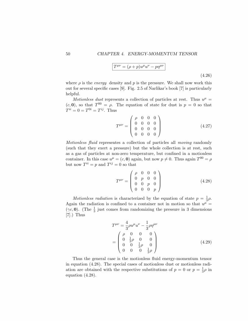
Tµν = (ρ+ p)uµuν − pηµν

(4.26)

where ρ is the energy density and p is the pressure. We shall now work thisout for several specific cases [9]. Fig. 2.5 of Narlikar’s book [7] is particularlyhelpful.

Motionless dust represents a collection of particles at rest. Thus uµ =(c,0), so that T 00 = ρ. The equation of state for dust is p = 0 so thatT ii = 0 = T 0i = T ij . Thus

Tµν =

ρ 0 0 00 0 0 00 0 0 00 0 0 0

(4.27)

Motionless fluid representes a collection of particles all moving randomly(such that they exert a pressure) but the whole collection is at rest, suchas a gas of particles at non-zero temperature, but confined in a motionlesscontainer. In this case uµ = (c,0) again, but now p 6= 0. Thus again T 00 = ρbut now T ii = p and T ij = 0 so that

Tµν =

ρ 0 0 00 p 0 00 0 p 00 0 0 p

(4.28)

Motionless radiation is characterized by the equation of state p = 13ρ.

Again the radiation is confined to a container not in motion so that uµ =(γc,0). (The 1

3 just comes from randomizing the pressure in 3 dimensions[7].) Thus

Tµν =43ρuµuν − 1

3ρηµν

=

ρ 0 0 00 1

3ρ 0 00 0 1

3ρ 00 0 0 1

3ρ

(4.29)

Thus the general case is the motionless fluid energy-momentum tensorin equation (4.28). The special cases of motionless dust or motionless radi-ation are obtained with the respective substitutions of p = 0 or p = 1

3ρ inequation (4.28).

4.5. CONTINUITY EQUATION 51

4.5 Continuity Equation

In classical electrodynamics the fourcurrent density is jµ ≡ (cρ, j) and thecovariant conservation law is ∂µj

µ = 0 which results in the equation ofcontinuity ∂ρ

∂t + 5.j = 0. This can also be obtained from the Maxwellequations by taking the divergence of Ampere’s law. (do Problems 4.1and 4.2) Thus the four Maxwell equations are entirely equivalent to onlythree Maxwell equations plus the equation of continuity.

We had a similar situation in Chapters 1 and 2 where we found that thevelocity and acceleration equations imply the conservation equation. Thusthe two velocity and acceleration equations are entirely equivalent to onlythe velocity equation plus the conservation law.

In analogy with electrodynamics the conservation law for the energy-momentum tensor is

Tµν;ν = 0 (4.30)

In the next chapter we shall show how equation (2.1) can be derived fromthis.

4.6 Interacting Scalar Field

We represent the interaction of a scalar field with a scalar potential V (φ).Recall our elementary results for L = T − V = 1

2mq2i − V (qi) for the coordi-

nates qi. These discrete coordinates qi have now been replaced by continuousfield variables φ(x) where φ has replaced the generalized coordinate q andthe discrete index i has been replaced by a continuous index x. Thus V (qi)naturally gets replaced with V (φ) where φ ≡ φ(x).

Thus for an interacting scalar field we simply tack on −V (φ) to the freeKlein-Gordon Lagrangian of equation (4.19) to give

L =12

(∂µφ∂µφ−m2φ2)− V (φ)

≡ LO + LI (4.31)

where LO ≡ LKG and LI ≡ −V (φ). Actually the Lagrangian of (4.31)refers to a minimally coupled scalar field as opposed to conformally coupled[21] (Pg. 276). It is important to emphasize that V (φ) does not containderivative terms such as ∂µφ. Thus the covariant momentum density andcanonical momentum remain the same as equations (4.20) and (4.21) for the


free particle case namely Πα = ∂αφ and π = φ. Solving the Euler-Lagrangeequations now gives

(22 +m2)φ+ V ′ = 0φ−52φ+m2φ+ V ′ = 0 (4.32)

with

V ′ ≡ dV

dφ(4.33)

The energy-momentum tensor is the same as for the free particle case,equation (4.24), except for the addition of gµνV (φ) as in

Tµν = ∂µφ∂νφ− gµν [12

(∂αφ∂αφ−m2φ2)− V (φ)] (4.34)

yielding the Hamiltonian density the same as for the free particle case, equa-tion (4.25), except for the addition of V (φ) as in

H ≡ T00 =12φ2 +

12

(5φ)2 +12m2φ2 + V (φ)

=12

[Π2 + (5φ)2 +m2φ2] + V (φ). (4.35)

The purely spatial components are Tii = ∂iφ∂iφ−gii[12(∂αφ∂αφ−m2φ2)−

V (φ)] and with gii = −1 (i.e. assume Special Relativity NNN) we obtain

Tii =12φ2 +

12

(5φ)2 − 12m2φ2 − V (φ) (4.36)

Note that even though Tii has repeated indices let us not assume∑i is

implied in this case. That is Tii refers to Tii = T11 = T22 = T33 and notTii = T11 + T22 + T33. Some authors (e.g Serot and Walecka [34]) do assumethe latter convention and therefore will disagree with our results by 1

3 .Let us assume that the effects of the scalar field are averaged so as

to behave like a perfect (motionless) fluid. In that case, comparing equa-tion (4.28), we make the identification [13, 34]

E ≡ ρ ≡< T00 > (4.37)

andp ≡< Tii > (4.38)

4.7. COSMOLOGY WITH THE SCALAR FIELD 53

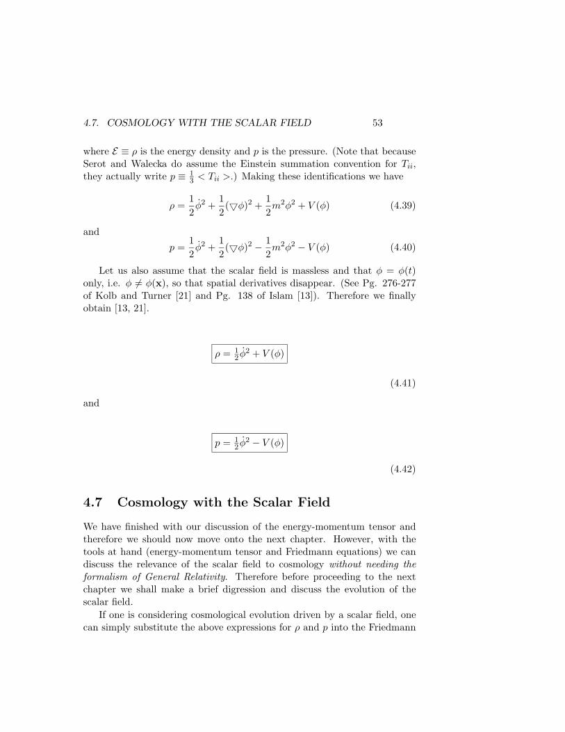
where E ≡ ρ is the energy density and p is the pressure. (Note that becauseSerot and Walecka do assume the Einstein summation convention for Tii,they actually write p ≡ 1

3 < Tii >.) Making these identifications we have

ρ =12φ2 +

12

(5φ)2 +12m2φ2 + V (φ) (4.39)

and

p =12φ2 +

12

(5φ)2 − 12m2φ2 − V (φ) (4.40)

Let us also assume that the scalar field is massless and that φ = φ(t)only, i.e. φ 6= φ(x), so that spatial derivatives disappear. (See Pg. 276-277of Kolb and Turner [21] and Pg. 138 of Islam [13]). Therefore we finallyobtain [13, 21].

ρ = 12 φ

2 + V (φ)

(4.41)

and

p = 12 φ

2 − V (φ)

(4.42)

4.7 Cosmology with the Scalar Field

We have finished with our discussion of the energy-momentum tensor andtherefore we should now move onto the next chapter. However, with thetools at hand (energy-momentum tensor and Friedmann equations) we candiscuss the relevance of the scalar field to cosmology without needing theformalism of General Relativity. Therefore before proceeding to the nextchapter we shall make a brief digression and discuss the evolution of thescalar field.

If one is considering cosmological evolution driven by a scalar field, onecan simply substitute the above expressions for ρ and p into the Friedmann


and acceleration equations (1.29) and (1.30) to obtain the time evolution ofthe scale factor as in

H2 ≡ (R

R)2 =

8πG3

[12φ2 +

12

(5φ)2 +12m2φ2 + V (φ)]− k

R2+

Λ3

(4.43)

andR

R= −4πG

3[12φ2 +

12

(5φ)2 − 12m2φ2 − V (φ)] +

Λ3

(4.44)

The equation for the time evolution of the scalar field is obtained either bytaking the time derivative of equation (4.43) or more simply by substitutingthe expression for ρ and p in equations (4.41) and (4.42) into the conservationequation (2.1) to give

φ+ 3H[φ+(5φ)2

φ] +m2φ+ V ′ = 0. (4.45)

Note that this is a new Klein-Gordon equation quite different to equation (4.32).The difference occurs because we have now incorporated gravity via theFriedmann and conservation equation. We shall derive this equation againin Chapter 7.

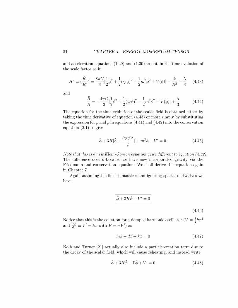
Again assuming the field is massless and ignoring spatial derivatives wehave

φ+ 3Hφ+ V ′ = 0

(4.46)

Notice that this is the equation for a damped harmonic oscillator (V = 12kx

2

and dVdx ≡ V ′ = kx with F = −V ′) as

mx+ dx+ kx = 0 (4.47)

Kolb and Turner [21] actually also include a particle creation term due tothe decay of the scalar field, which will cause reheating, and instead write

φ+ 3Hφ+ Γφ+ V ′ = 0 (4.48)


4.7.1 Alternative derivation

We can derive the equation of motion (4.46) for the scalar field in a quickermanner [29] (Pg. 73), but this derivation only seems to work if we set m = 0and 5φ = 0 at the beginning. (Exercise: find out what goes wrong if m 6= 0and 5φ 6= 0.)

Consider a Lagrangian for φ which already has the scale factor built intoit as

L = R3[12

(∂µφ∂µφ−m2φ2)− V (φ)] (4.49)

The R3 factor comes from√−g = R3 for a Robertson-Walker metric. This

will be discussed in Chapter 7. Notice that it is the same factor whichsits outside the Friedmann Lagrangian in equation (2.20). The equation ofmotion is (do Problem 4.3)

φ−52φ+ 3Hφ+m2φ+ V ′ = 0 (4.50)

which is different to (4.45). (NNNN why ???) However if m = 0 and5φ = 0it is the same as (4.46).

Let’s only consider

L = R3[12φ2 − V (φ)] (4.51)

which results from setting m = 0 and 5φ = 0 in (4.49). The equation ofmotion is

φ+ 3Hφ+ V ′ = 0 (4.52)

Notice how quickly we obtained this result rather than the long procedureto get (4.46). We didn’t even use the energy-momentum tensor. Also realizethat because5φ = 0 the above Lagrangian formalism is really no different toour old fashioned formalism where we had qi(t). Here we have only φ = φ(t)(not φ = φ(x)), and so we only have i = 1, i.e. qi ≡ φ.

Identifying the Lagrangian as [29] L = R3(T − V ) we immediately writedown the total energy density ρ = T + V = 1

2 φ2 + V (φ). Taking the time

derivative ρ = φφ + V ′φ = −3Hφ2 from (4.46) and substituting into theconservation equation (2.1), ρ = −3H(ρ + p) we obtain the pressure asp = 1

2 φ2 − V (φ). Thus our energy density and pressure derived here agree

with our results above (4.39) and (4.40). Notice that the pressure is nothingmore than p = L

R3 . [29].


4.7.2 Limiting solutions

Assuming that k = Λ = 0 the Friedmann equation becomes

H2 ≡ (R

R)2 =

8πG3

(12φ+ V ) (4.53)

This equation together with equation (4.46) form a set of coupled equationswhere solutions give φ(t) and R(t). We solve the coupled equations in thestandard way by first eliminating one variable, then solving one equation,then substituting the solution back into the other equation to solve for theother variable. Let’s write equation (4.46) purely in terms of φ by eliminatingR which appears in the form H = R

R . We eliminate R by substituting Hfrom (4.53) into (4.46) to give

φ+√

12πG(φ2 + 2V )φ+V’=0

φ2 + 2φV ′ − 12πG(φ2 + 2V )φ2 + V ′2 = 0 (4.54)

Notice that this is a non-linear differential equation for φ, which is difficultto solve in general. In this section we shall study the solutions for certainlimiting cases. Once φ(t) is obtained from (4.54) it is put back into (4.53)to get R(t).

Potential Energy=0

Setting V = 0 we then have ρ = 12 φ

2 = p. Thus our equation of state is

p = ρ (4.55)

or γ = 3.With V = V ′ = 0 we have

φ2 +√

12πGφ2 = 0 (4.56)

which has the solution (do problem 4.4)

φ(t) = φo +1√

12πGln[1 +

√12πGφ(t− to)] (4.57)


(Note that the solution is equation (9.18) of [29] is wrong.) Upon substitut-ing this solution back into the Friedmann equation (4.53) and solving thedifferential equation we obtain (do problem 4.5)

R(t) = Ro[1 +√

12πGφo(t− to)]1/3. (4.58)

This result may be understood from another point of view. Writing theFriedmann equations as

H2 ≡ (R

R)2 =

8πG3

ρ (4.59)

andρ =

α

Rm(4.60)

then the solution is alwaysR∝t2/m (4.61)

which always gives

ρ ∝ 1t2. (4.62)

Ifρ = constant (4.63)

(corresponding to m = 0) then the solution is

R∝et (4.64)

(do problem 4.6). Note that for m < 2, one obtains power law inflation.For ordinary matter (m = 3), or radiation (m = 4) we have R ∝ t2/3 andR ∝ t1/2 respectively. Returning to the scalar field solution (4.57) the densityis ρ = 1

2 φ2 for V = 0. Thus

φ(t) =φo

1 +√

12πGφo(t− to)(4.65)

combined with ( RRo )3 = 1 +√

12πGφo(t− to) from (4.58) yields

φ(t) =φoR

3o

R3(4.66)

to give the density


ρ = 12φ2oR

6o

R6

(4.67)

corresponding to m = 6 and thus R ∝ t1/3 in agreement with (4.58). Notealso that this density ρ ∝ 1

R6 also gives ρ ∝ 1t2

.Thus for a scalar field with V = 0, we have p = ρ (γ = 3) and ρ ∝ 1

R6 .Contrast this with matter for which p = 0(γ = 0) and ρ ∝ 1

R3 or radiationfor which p = 1

3ρ (γ = 1/3) and ρ ∝ 1R4 .

However equation (4.67) may not be interpreted as a decaying Cosmo-logical Constant because p 6= ρ (see later).

Kinetic Energy=0Here we take φ = φ = 0, so that ρ = V and p = −V giving

p = −ρ (4.68)

or γ = −3 which is a negative pressure equation of state. Our equation ofmotion for the scalar field (4.54) becomes

V ′ = 0 (4.69)

meaning thatV = Vo (4.70)

which is constant. Substituting the solution into the Friedmann equation(4.53) gives

H2 = (R

R)2 =

8πG3

Vo (4.71)

which acts as a Cosmological Constant and which has the solution (do prob-lem 4.7)

R(t) = Roe√

8πG3Vo(t−to) (4.72)

which is an inflationary solution, valid for any V .

Warning

We have found that if k = Λ = 0 and if ρ ∝ 1Rm then R∝t2 for any

value of m. All of this is correct. To check this we might substitute into theFriedmann equation as

H2 = (R

R)2 ∝ 1

t2(4.73)


and say RR ∝ 1

t giving∫ 1RdRdt dt ∝

∫ dtt which yields lnR ∝ lnt and thus

R ∝ t2/m. The result R ∝t is wrong because we have left out an importantconstant.

Actually if RR = c

t then lnR = c ln t = ln tc giving R ∝ tc instead of R∝t.Let’s keep our constants then. Write ρ = d2

Rm then R = (md2 )2/mt2/m

and ρ = d2

(md2

)2t2= (2/m)2

t2. Substituting into the Friedmann equation gives

( RR)2 = (2/m)2

t2or R

R = (2/m)t with the above constant C = 2

m yieldingR ∝t2/m in agreement with the correct result above.

The lesson is be careful of constants when doing back-of-the-envelopecalculations.

4.7.3 Exactly Solvable Model of Inflation

Because (4.54) is a difficult non-linear equation, exactly solvable models arevery rare. We shall examine the model of Barrow [35] which can be solvedexactly and leads to power law inflation. The advantage of an exactly solv-able model is that one can develop ones physical intuition better. Barrow’smodel [35] is briefly introduced by Islam [13].

Any scalar field model is specified by writing down the potential V (φ).Barrow’s potential is

V (φ) ≡ βe−λφ (4.74)

where β and λ are constants to be determined. Barrow [35] claims that aparticular solution to (4.54) is (which was presumably guessed at, ratherthen solving the differential equation)

φ(t) =√

2Alnt (4.75)

where√

2A is just some constant. We check this claim by substituting (4.74)and (4.75) into (4.54). From this we find (do problem 4.9) that

λ =√

2A

(4.76)

andβ = −A (4.77)

orβ = A(24πGA− 1) (4.78)


Note that Barrow is wrong when he writes λA =√

2. Also he uses unitswith 8πG = 1, so that the second solution (4.78), he writes correctly asβ = A(3A− 1). Also Barrow doesn’t use the first solution (4.77) for reasonswe shall see shortly.

Having solved for φ(t) we now substitute into (4.53) to solve for R(t).(Recall φ(t) and R(t) are the solutions we seek to our coupled equations(4.46) and (4.53).) Substituting V = Λ

t2and φ =

√2At (see solution to

problem 4.9) we have

H2 ≡ (R

R)2 =

8πG3

(12

2At2

+β

t2) =

8πG3

(A+ β)1t2

(4.79)

giving an equivalent density

ρ =A+ β

t2(4.80)

Clearly we see why we reject the first solution (4.77) with β = −A. It wouldgive zero density. Using the second solution (4.78) with β = A(24πGA− 1)yields

ρ =24πGA2

t2. (4.81)

Solving the Friedmann equation (4.79) gives

R∝t8πGA (4.82)

where D is some constant. Setting 8πG ≡ 1 we have

R∝tA (4.83)

in agreement with Barrow’s solution. Power law inflation results for

A > 1. (4.84)

Inverting the solution (4.83) we have t2 = C ′R2/A where C ′ is some constant.Substituting into (4.81) we have

ρ ∝ 1R2/A

(4.85)

which corresponds to a Weak decaying Cosmological Constant. (See sections4.7.4 and 4.7.5) For the inflationary result A > 1 we have 2

A ≡ m < 2 whichcorresponds to the quantum tunneling solution!!

Note of course that (4.85) can also be obtained via ρ = 13 φ

2+V. We haveV= β

t2∝ 1

R2/A and φ =√

2At giving φ2 ∝ 1

R2/A .


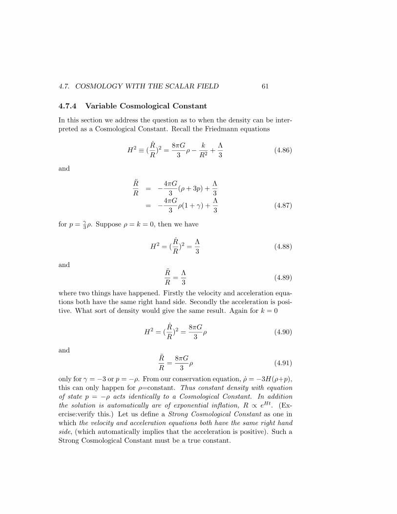
4.7.4 Variable Cosmological Constant

In this section we address the question as to when the density can be inter-preted as a Cosmological Constant. Recall the Friedmann equations

H2 ≡ (R

R)2 =

8πG3

ρ− k

R2+

Λ3

(4.86)

and

R

R= −4πG

3(ρ+ 3p) +

Λ3

= −4πG3

ρ(1 + γ) +Λ3

(4.87)

for p = γ3ρ. Suppose ρ = k = 0, then we have

H2 = (R

R)2 =

Λ3

(4.88)

andR

R=

Λ3

(4.89)

where two things have happened. Firstly the velocity and acceleration equa-tions both have the same right hand side. Secondly the acceleration is posi-tive. What sort of density would give the same result. Again for k = 0

H2 = (R

R)2 =

8πG3

ρ (4.90)

andR

R=

8πG3

ρ (4.91)

only for γ = −3 or p = −ρ. From our conservation equation, ρ = −3H(ρ+p),this can only happen for ρ=constant. Thus constant density with equationof state p = −ρ acts identically to a Cosmological Constant. In additionthe solution is automatically are of exponential inflation, R ∝ eHt. (Ex-ercise:verify this.) Let us define a Strong Cosmological Constant as one inwhich the velocity and acceleration equations both have the same right handside, (which automatically implies that the acceleration is positive). Such aStrong Cosmological Constant must be a true constant.


On the other hand we can imagine densities that still give a positiveacceleration (i.e. inflation) but do not normally give the velocity and accel-eration with the same right hand side. Examining (4.54) indicates that theacceleration is guarenteed to be positive if γ < −1 giving p < −1

3ρ. (Recallthat the exponential inflation above required γ = −3, which is consistentwith the inequality.) Thus negative pressure gives inflation. (Although notall negative pressure gives inflation, e.g. p = −1

4ρ.) The inflation due toγ < −1 will not be exponential inflation, but something weaker like per-

haps power law inflation. Let us define a Weak Cosmological Constant asone which arises from negative pressure (actually p < −1

3ρ) to give a positiveacceleration (inflation) only. The velocity and acceleration equations neednot have the same right hand side.

Recall that ordinary matter and radiation, or any positive pressure equa-tion of state, neccesarily leads to negative acceleration (with Λ = 0). Thuspositive pressure leads to attractive gravity. However positive accelerationimplies a repulsive gravity or antigravity. Thus negative pressure (actuallyp < −1

3ρ) leads to antigravity. This is why we wish to use the term weak Cos-mological Constant (even though right hand sides are not the same) becauseit is consonant with antigravity.

Let us summarize. We consider ρ alone with Λ ≡ 0. For

R > 0⇒ γ < −1 and ρ =anything (e.g. ρ = ρ(R) or ρ =constant)R > 0 and ρ =constant⇒ γ = −3

For γ < −1, ρ behaves as a weak Cosmological Constant and for γ = −3,ρ behaves as a Strong Cosmological Constant.

Finally let us emphasize that it is perfectly legitimate to consider a WeakCosmological Constant as a real Cosmological Constant. Einstein’s originalmotivation in introducing Λ was to obtain a static universe. Thus all hewanted was a antigravity term; i.e. all he wanted was a weak CosmologicalConstant. It “accidentally” happened that the right hand sides turned outto be equal, giving a strong Λ.

Interpreting ρ as a Cosmological Constant leads us to expect that aweak Cosmological Constant can vary. This follows from ρ=anything above.i.e. ρ=constant or ρ = ρ(R) giving a variable function. (But a strongCosmological Constant cannot vary).


4.7.5 Cosmological constant and Scalar Fields

Refer back to the density and pressure of the scalar field in equations (4.41))and (4.42). We had

ρ =12φ2 + V (φ)

and

ρ =12φ2 − V (φ).

For the case where PE = V = 0 we have p = ρ. The pressure is positiveand therefore equation (4.67), ρ ∝ 1

R6 , cannot be interpreted as a (variable)Cosmological Constant.

For the case where KE = 12 φ

2 = 0 we have p = −ρ meaning that ρ canbe interpreted as a Strong Cosmological Constant. (We found V ′ = 0 andthus ρ = V = constant = Vo and p = −Vo.)

These results are true in general (assuming m = ∇φ = 0) as we have notyet specified V (φ).

Let us now consider the Barrow model V (φ) = βe−λφ. we found thatφ(t) = 2

λ ln t and β = 2λ2 ( 6

λ2 − 1) for 8πG ≡ 1. Introducing A ≡ 2λ we can

re-write as β = A(3A − 1) and φ(t) =√

2A ln t and V (φ) = A(3A − 1)eφ2A .

Substituting we obtain

ρBarrow =3A2

t2(4.92)

and

ρBarrow =3A2

t2(2A3− 1) = (

2A3− 1)ρ (4.93)

the general equation of state is p = γ3ρ giving the Barrow equation of state

γBarrow =2A− 3 (4.94)

in equation (4.84) we concluded that power law inflation results for A > 1.Substituting this into (4.94) implies

γBarrow < −3 (4.95)

which we expect because power law inflation implies R > 0. thus for A > 1the Barrow pressure is negative with γ < −1 and thus ρBarrow = 3A2

t2cor-

responds to a Weak Cosmological Constant. Furthermore this CosmologicalConstant is variable and decays with time. in equation (4.85) we wrote thisas ρBarrow ∝ 1

R2/A .


4.7.6 Clarification

We wish to clarify the distinction between a Strong Cosmological Constant,a Weak Cosmological Constant and a Varying Cosmological Constant. AStrong Cosmological Constant occurs when the Friedmann equation are ofthe form

H2 ≡ (R

R)2 =

Λ3

(4.96)

and

−qH2 ≡ R

R=

Λ3

(4.97)

and comparing with

(R

R)2 =

8πG3

ρ (4.98)

R

R= −8πG

3(ρ+ 3p) (4.99)

leads us to conclude that the equation of state for a Strong CosmologicalConstant is p = −ρ, where we have identified Λ ≡ 8πGρv. The conservationequation

ρ = −3H(ρ+ p) (4.100)

leads us to conclude that Λ ≡ 8πGρv=constant for a Strong CosmologicalConstant.

A Variable Cosmological Constant Λ(R), can also be considered but theequation cannot be like (4.96) and (4.97) with no ρ term. As we shall see be-low a Varying Cosmological Constant automatically involves matter creation(existence of a ρ term). Thus Λ(R) cannot be written down in the Friedmannequation without also writing ρ. Thus for a Varying Cosmological Constant(let k = 0) we have

H2 ≡ (R

R)2 =

8πG3

ρ+Λ(R)

3(4.101)

and

−qH2 ≡ R

R= −4πG

3(1 + γ)ρ+

Λ3

(4.102)

One can easily show that the conservation equation becomes

ρ+ ρv =-3H(ρ+p) =−H(3+γ)ρ


(4.103)

(do Problem 4.10). Other ways of writing this are (see equations 2.1-2.7).

d(ρR3)dt

+ pdR3

dt+R3ρv = 0 (4.104)

d(ρR3+γ)dt

+R3+γ ρv = 0 (4.105)

ρ′ + ρ′v = − 3R

(ρ+ p) (4.106)

d(ρR3)dR

+ 3pR2 +R3ρ′v = 0 (4.107)

1R3+γ

d(ρR3+γ)dR

= −ρ′v (4.108)

The last equation show clearly that if ρv 6= 0 (i.e. ρv 6= constant) thenmatter or radiation is created or destroyed. This is why we cannot write(4.96) and (4.97) if Λ is allowed to vary. We must include particle creationterms as in (??) and (4.102).

For a Variable Cosmological Constant the same term Λ(R)3 appears in

both right hand sides of the Friedmann equation (4.101) and (4.102). How-ever we don’t know its equation of state. Also γ can be anything and thusρv can lead to creation of matter, radiation or anything else. Further Λ(R)can vary.

Both a Strong and Weak Cosmological Constant have well defined equa-tion of state, both with (different) negative pressure. A Weak CosmologicalConstant can vary but the right hand sides of the Friedmann equations differ.

Thus we see that we have 3 different types of Cosmological Constantnamely, Strong, Weak, and Variable, each with both similar and dissimiliarproperties. These are summarize in the Table.

4.7.7 Generic Inflation and Slow-Roll Approximation

We shall first discuss features that are common to many models of inflationbased on scalar fields [21]. These models typically have a large region of thepotential where the potential is flat (slow-roll region) and then a harmonic


Weak Strong VariableRight Hand Sidesof Velocity and Different same Same (but must include ρ)

Acceleration Eqns.

Eqn. State p < −13ρ p = −ρ Unknown

Λ = 8πGρv Variable Constant Variable

Table 4.1: Properties of 3 types of Cosmological Constants

region where the potential looks similar to an oscillatior (rapid oscillationregion). Such a potential is shown in Fig 4.1.

Let us first analyze this situation from a simple physics point of view. IfFig 4.1 were actually a plot of V (x) versus x the equation of motion wouldbe

mx+ bx+ V ′ = 0 (4.109)

which, for V = 12kx

2 or V ′ = kx would represent a damped harmonic oscil-lator, which indeed is the case in the rapid oscillation region. In the slowroll regime we have V ≈constant or V = Vo − Cx where C is small, givingV ′ = −C. The physical situation would represent a ball rolling down a hillwith friction into a valley [21].

In the slow roll regime friction dominates and the ball moves at terminalvelocity [21], x=constant and x doesn’t change much so that x = 0. This isthe slow roll regime we have

bx+ V ′ = 0 (4.110)

and for V = Vo − Cx we havebx≈C (4.111)

When the ball finally reaches the valley we are back to the full equation(4.109) where V ′ ≡ kx so that the ball experiences rapid, damped oscilla-tions.

Let’s return to the scalar field equations which are (for Λ = k = 0)

H2 ≡ (R

R)2 =

8πG3

(12φ+ V ) (4.112)


andφ+ 3Hφ+ V ′ = 0 (4.113)

where the friction term 3H is due to the expansion of the universe [21]. Basedon analogy with the rolling ball, the slow roll approximation (φ ≈constant,φ ≈ 0) is

3Hφ+ V ′ ≈ 0 (4.114)

In addition, the slow roll region is characterized by a small kinetic energy12 φ

2 << V , so that

H2 ≈ 8πG3

Vo ≈ constant (4.115)

For the rolling ball we only had one equation, but here we have two equations(4.114) and (4.115) involved in the slow roll approximations. The slow rollequation can also be obtained directly from equation (4.54) where we setφ2 << 2Vo and φ ≈ 0 to give√

24πGVoφ+ V ′ = 0 (4.116)

which is consistent with combining (4.114) and (4.115). Normally we wouldhave the formula for V(φ) and solve (4.116) or (4.54) first for φ(t) and thensubstitute our answer into the Friedmann equation to obtain R(t). Howeverwe have not yet specified V (φ). We have specified that we are in a slow rollregime thus making (4.115) valid which we can solve directly for R(t) givingan exponential inflationary solution

R(t)≈Roet√

8πG3VO (4.117)

Thus, no matter what V (φ) is, the slow regime always give approximatelyexponential inflation.

To obtain φ(t) we must specify V (φ) even in the slow-roll regime.

4.7.8 Chaotic Inflation in Slow-Roll Approximation

The Chaotic inflation model is defined by the potential

V (φ) =12m2φ2 (4.118)

which is exactly analogous to the harmonic oscillator potential V (x) = 12kx

2.


Using Vo = 12m

2φ2o the slow roll solution (4.117) becomes

R(t) = Roet√

4π3

√Gmφ

= Roet√

4π3

mMp

φ (4.119)

where G ≡ 1M2p

is in agreement with equation (9.23) of Madsen [29]. Havingspecified V (φ) in (4.118) we can solve (4.116), which

φ = − 1√24πG

V ′√Vo

(4.120)

orφ

φ= − m√

12πG1φo

(4.121)

This gives

φ(t) = φoe− m

φo√

12πGt

= φoe− mMp

φo√

12πt

= φo −mMp√

12πt (4.122)

is the slow roll region in agreement with equation (9.25) of Madsen [29]. Form << Mp or for short times we see that φ(t) will be approximately constant,or slowing rolling. We see that φ(t) is a decaying exponential in time. Thusthere will be a “half-life” or “lifetime” associated with slow roll which wedefine as

τ =φo√

12πmMp

(4.123)

When t = τ we see that φ = φo1e . That is the amplitude is reduced by the

factor 1e We expect that the slow roll approximation will be valid for t < τ .

Our solution of φ(t) in (4.122) came from solving (4.116). We can alsoobtain φ(t) slightly differently. Let’s not assume V = Vo=constant, but onlythat φ2 << 2V and φ ≈ 0. Then instead of (4.116) we have

√24πGV φ+ V ′ = 0 (4.124)

which, for chaotic inflation becomes√

12πGmφφ+m2φ = 0 (4.125)


orφ = − m√

12πG(4.126)

which has the solution

φ(t) = φo −m√

12πGt

= φo −mMp√

12πt (4.127)

in agreement with (4.122) for short time.We can further investigate the validity of the slow roll approximation by

evaluating the potential as a function of time and checking that it is constantfor short times. We do this by substituting our solution for φ(t) back intothe potential. We get

V =12m2φ2 =

12m2φ2

oe− mMp

φo√

3πt

≈ 12m2φo(φo −

mMp√3π

t) (4.128)

Thus we see that for m << Mp or for short times the potential is indeedconstant.

For short times (or for m << Mp) we have verified that φ and V areapproximately constant. This means that φ ≈ 0 and ρ ≈ Vo which giveexponential inflation. (Also p ≈ −Vo, so that p = −ρ).

In order to solve the horizon, flatness and monopole problems, mostmodels require a high degree of inflation typically amounting to about 60e-folds [21]. Given R(t) = Roe

Ht, the number of e-folds after time t is

N = ln(R(t)Ro

) = Ht. (4.129)

(Actually a better formula is given in equation (8.26) of the book by Kolband Turner [21] (pg.278)). After one lifetime τ , the number of e-folds is

N = Hτ =√

4π3m

Mpφoφo√

12πmMp

= 4πφ2o

M2p

(4.130)

where H =√

4π3

mMpφo taken from (4.119) and τ is from (4.123). Thus the

requirement N ≥ 60 yields

N ≥ 60 ⇒ φo ≥√

5Mp. (4.131)


Notice how the flatness problem is solved in inflation. We have H2 ≡ ( RR)2 =8πG

3 ρ− kR2 ≈ 8πG

3 Vo − kR2 . During inflation (slow roll) Vo stays constant but

by the end of inflation R = Roe60 or 1

R2 = 1R2oe−120. The term k

R2 has

dropped by e−120, whereas Vo has remained constant. Thus the term kR2 is

entirely negligible. Inflation does not give k = 0, but rather gives kR2 ≈ 0

which is equivalent to k = 0. This is an improtant distinction. The universecan have k = 0 or k = +1 or k = −1. No matter what the value of k, it getsdiluted by inflation and is equivalent to a universe with k = 0. thus withinour horizon the universe is flat. Quantum cosmology predict that a universewhich arises via tunnelling must have k = +1. This is perfectly OK withinflation which simply dilutes the curvature.

Quantum tunnelling requires k = +1. Inflation actually says nothingabout the value of k. It simply predicts that k

R2 ≈ 0 at the end of inflation.On Earth, the reason many people believe the Earth is flat is because

we cannot see beyond the horizon. Up to the horizon it looks flat. If wecould see beyond the horizon we would see the curvature. Similarly for ouruniverse. According to inflation the size of the universe is much larger thenthe distance to the horizon ( i.e. as far as we can see) the universe looksflat becuase k

R2 is negligible. If we could see beyond the horizon we wouldsee the curvature. And quantum tunnelling predicts that what we would seewould be a universe of positive curvature.

Cosmological Constant associated with Chaotic InflationLet us now calculate the density as a function of R. We solve (4.119) for

t = t(R) as

t =√

34π

Mp

mφoln(

R

Ro). (4.132)

Substituting into (4.122) we have

φ(R) = φo(RoR

)M2p

4πφ2o (4.133)

and with V (φ) = 12m

2φ2 we have

V (R) =12m2φ2

o(RoR

)M2p

2πφ2o . (4.134)

Also from (4.122)

φ(t) = −mMp√12π

e− mMp

φo√

12π t (4.135)


so that

φ(R) = −mMp√12π

(RoR

)M2p

4πφ2o . (4.136)

Finally evaluating ρ = 12 φ

2 + V we have

ρ(R) =12m2(

M2p

12π+ φ2

o)(RoR

)M2p

2πφ2o . (4.137)

Thus

ρ(R) ∝ 1Rm

where m ≡M2p

2πφ2o

. (4.138)

Recall previously that an inflationary solution requires m < 2, yielding

φo >Mp√

4π= 0.3 Mp (4.139)

which is entirely consistent with (4.131)!What is the equation of state? using p = 1

2 φ2 − V we obtain

p =12m2(

M2p

12π− φ2

o)(RoR

)M2p

2πφ2o . (4.140)

The question is, is the pressure negative? We find that for inflation to occurwe need φo >

Mp√4π

. Write this as

φo = `Mp√

4πwith ` > 1 (4.141)

Thus the density becomes

ρ(R) =m2M2

p

8π(13

+ `2)(RoR

)m (4.142)

and

p(R) =m2M2

p

8π(13− `2)(

RoR

)m (4.143)

Defining κ ≡ m2M2p

8π (RoR )m, we write ρ = (13 + `2)κ and p = (1

3 − `2)κ, givingp = 1−3`2

1+3`2ρ. The requirement ` > 1 yields

p < −12ρ (4.144)


which means negative pressure! Writing p = γ3ρ gives

γ = −32. (4.145)

These results are in agreement with our previous constraints that in orderto have positive R (inflation) we needed p < 1

3ρ or γ < −1.Our chaotic inflation model is the slow roll approximation gives negative

pressure (but not p = −ρ) and corresponds to a Weak Decaying CosmologicalConstant!

4.7.9 Density Fluctuations

An important result that we shall use without proof is that fluctuations ofthe scalar field are given approximately by

δφ ≈ H2π

(4.146)

this result is discussed by Linde [36] (Pg.17,50), Kolb and Turner [21](Pg.284),Collins, Martin and Squires [37] (Pg.410) and by Dolgov, Sazhin and Zel-dovich [38].

Using ρ = 12 φ

2+V(φ) we have dρdφ = V ′(φ) or

δρ = V ′δφ≈V ′ H2π

(4.147)

which, upon assuming φ = 0, gives

δρ

ρ=

√2

3πGV ′2

V=√

23π

V ′

Mp

√V

(4.148)

where we have used G ≡ 1M2p

. For the chaotic inflation model, V = 12m

2φ2

this yieldsδρ

ρ=√

43π

m

Mp. (4.149)

This is an intensely important formula often written as

δρ

ρ≈m√G =

m

Mp(4.150)


the density fluctuations observed by COBE are δρρ ≈ 10−5 yielding m =

10−5Mp.The above formula is not very useful for the Barrow model where a well

defined inflation means m ≡ minflation is not present. In that case theformula is written more usefully as [?, ?, ?]

δρ

ρ=ρinflation

ρp(4.151)

4.7.10 Equation of State for Variable Cosmological Constant

In this section we wish to demonstrate that Variable Cosmological Constantmodels have negative pressure [?, ?, ?].

Firstly if one assumesp ≡ γ

3ρ (4.152)

then the conservation law follows as

1R3+γ

d

dR(ρR3+γ) = −ρ′v. (4.153)

Let’s assume thatρv ≡

α

Rm= ρvo(

RoR

)m. (4.154)

Integrating the conservation law we have

ρ =A

R3+γ+ χρv (4.155)

whereχ ≡ m

3 + γ −m (4.156)

and A is a constant give by

A = (ρo − χρvo)R3+γo . (4.157)

The pressure is

p =γ

3A

R3+γ+γ

3m

3 + γ −mρv (4.158)

This looks like bad news. Assuming that ρv dominate over the first termat some stage of evolution, it looks like the pressure only get negative form> 3 + γ. However, there are two things to keep in mind. Firstly, the


pressure p is not the pressure of radiation or matter or vacuum becauseρ = A

R3+γ +χρ, and p = γ3ρ. The pressure that we would want to be negative

would be the vacuum pressure pv, which we shall work out below. Secondly,the key point is not as much having p negative but rather having R positive.The equation

−qH2 ≡ R

R= −4πG

3(ρ+ 3p) +

8πG3

ρv (4.159)

can still give postive R even if p is not negative, because the ρv term has tobe considered. The Friedmann equation is

H2 ≡ (R

R)2 =

8πG3

(ρ+ ρv)−k

R2(4.160)

Let us evaluate the right hand sides of these two equations (4.159) and(4.160).

From (4.155) we have

H2 ≡ (R

R)2 =

8πG3

[A

R3+γ+ (χ+ 1)ρv]−

k

R2(4.161)

where

χ+ 1 =3 + γ

3 + γ −m. (4.162)

Also assuming p= γ3ρ we have

−qH2 ≡ R

R= −4πG

3(1 + γ)(

A

R3+γ+ χρv) +

8πG3

ρv (4.163)

= −4πG3

[1 + γ)A

R3+γ+

(3 + γ)(m− 2)3 + γ −m ρv]. (4.164)

Define

θ ≡ (3 + γ)(m− 2)3 + γ −m (4.165)

we see that θ is always negative for m < 2! Thus if the vacuum term domi-nates equation (4.164) then R will be positive for m < 2. This agrees withour previous consideration that if ρ = α

Rm dominates the velocity equationthen m < 2 leads to inflation.

Note however that θ can be negative for other values of m as shown inTable 4.2.


m θ(γ = 0) θ(γ = 1)0.5 -1.8 -1.71 -1.5 -1.3

1.5 -1.0 -0.82 0 0

2.5 3.0 1.333 ∞ 44 -6 ∞5 -4.5 -126 -4 -8

Table 4.2: θ as a function of γ and m

Having established that a decaying Cosmological Constant can lead tonegative pressure, let us now work out the vacuum equation of state for adecaying Cosmological Constant. Looking at (4.161) let us define

ρ ≡ A

R3+γ(4.166)

andρv ≡ (χ+ 1)ρv =

3 + γ

3 + γ −mρv (4.167)

so thatρ+ ρv = ρ+ ρv (4.168)

giving

H2 ≡ (R

R)2 =

8πG3

(ρ+ ρv)−k

R2=

8πG3

(ρ+ ρv)−k

R2(4.169)

and from (4.164) we have

−qH2 ≡ R

R= −4πG

3[(1 + γ)ρ− 2ρv] (4.170)

= −4πG3

[(1 + γ)ρ+ (m− 2)ρv] (4.171)

which we would like to write as

−qH2 ≡ R

R= −4πG

3(ρ+ 3p)− 4πG

3(ρv + 3pv). (4.172)

This is achieved if we make the following defintions


p ≡ γ3 ρ

(4.173)

and

pv ≡ m−33 ρv ≡ γv

3 ρv ,

(4.174)

which is our vacuum equation of state for a decaying Cosmological Constant.We see that for m< 3 we have pv and γv negative. For a m < 2 we haveγv < −1 which we saw previously is the condition for inflation assumingvacuum domination of the density and pressure.

It is also satisfying to note that the equation of state for the non-vacuumcomponent (equation 4.173) is identical to the equation of state for a perfectfluid that we encountered for models without a Cosmological Constant.

Alternative DerivationOur definition of ρ and ρv above are not unique. We present alternative

definitions below which will give the same vacuum equation of state butdifferent for the non-vacuum component.

In equation (4.161) the density is

ρ+ ρv =A

R3+γ+ (χ+ 1)ρv

= (ρo − χρvo)(RoR

)3+γ + (χ+ 1)ρvo(RoR

)m

= ρo(RoR

)3+γ + ρvo[(χ+ 1)(RoR

)m − χ(RoR

)3+γ ] (4.175)

We previoulsy defined ρ ≡ AR3+γ and ρv ≡ (χ + 1)ρv. However we might

alternatively define

ρ ≡ ρo(RoR

)3+γ (4.176)

and

ρv ≡ ρvo[(χ+ 1)(RoR

)m − χ(RoR

3+γ

]

= (χ+ 1)ρv − χρvoρoρ (4.177)


still obtainingρ+ ρv = ρ+ ρv = ρ+ ρv. (4.178)

Assuming p = γ3ρ we have (compare to equation 4.171)

−qH2 ≡ R

R= −4πG

3[(1 + γ)ρ− 2ρv]

= −4πG3

[(1 + γ −mρvoρo

)ρ+ (m− 2)ρv] (4.179)

(where we have used the second expression in 4.177), which we would liketo write as

−qH2 ≡ R

R= −4πG

3(ρ+ 3p)− 4πG

3(ρv + 3pv). (4.180)

This is achieved if we make the following definitions

p ≡ γ−m ρvoρo

3 ρ ≡ Γ3 ρ

(4.181)

and

pv ≡ m−33 ρv = γv

3 ρv

(4.182)

4.7.11 Quantization

All of our proceeding work with the scalar field was at the classical level. Inthis section we wish to consider quantum effects.

In section (2.4.2) we dervied the wheeler-DeWitt equation in minisuper-space approximation. We began with the Lagrangian in equation (2.20)

L = −κR3[(R

R)2 − k

R2+

8πG3

(ρ+ ρv)] (4.183)

and identified the conjugate momentum p ≡ ∂L∂R

= −2κRR and derived theWheeler-DeWitt equation, after quantizing with p→ i ∂∂R , as

{− ∂2

∂R2+ 4κ2[kR2 − 8πG

3(ρ+ ρv)R4]}ψ = 0. (4.184)


Notice that our quantization ’didn’t do anything to the density.”In the work that we have done in the present chapter we have made

an effort to write the scalar field as a function of R, i.e. φ = φ(R) andusing ρ = 1

2 φ2 + V (φ) we have written as an effective density ρ(R) for

the scalar field. Our intention has been to simply insert this ρ(R) intothe Wheeler-DeWitt equation (4.184). In our work on inflation we foundthat for ρ ∝ 1

Rm dominating the Friedmann equation then inflation occursfor m < 2. If this density also dominates ρ + ρv in the Wheeler-DeWittequation, then a tunnelling potential will only be present for m < 2. Thusinflation and quantum tunnelling require the same condition. This leads usto the hypothesis that inflation and quantum tunnelling are identical! Or inother words, inflation is simply a classical description of quantum tunnelling.We call this hypothesis Quantum Inflation.

Quantum inflation is easy to validate for ordinary densities, either ρ orρv, that behave like ρ ∝ 1

Rm . With our discussion of the scalar field we havewritten ρφ ∝ 1

Rm so it would seem that the idea of quantum inflation alsoworks for scalar fields.

In our quantization procedure we ”didn’t do anything to the density.” Interms of scalar fields then this quantization procedure is different to whatother people do with quantization. The usual procedure [?, ?, ?, 20, 21] isto quantize φ and R seperately and arrive at a Wheeler- DeWitt equationin terms of both of these variables. Let us now study this procedure.

We begin with the Lagrangian

L = −κR3[(R

R)2 − k

R2] + 2π2R3[

12φ2 − V (φ)] (4.185)

where κ ≡ 3π4G .

From this one can deduce that

(R

R)2 =

8πG3

(12φ2 + V )− k

R2(4.186)

and alsoφ+ 3Hφ+ V ′ = 0 (4.187)

provided one uses RR = −4πG

3 (ρ + 3p) with ρ = 12 φ

2 + V and p = 12 φ

2 − V .(NNN see FE)

The canonical momenta are

ΠR ≡∂L

∂R= −2κRR (4.188)


andΠφ ≡

∂L

∂φ= 2π2R3φ. (4.189)

The Hamiltonian (H = piqi − L) becomes (using κ = 3π4G)

H = ΠRR+ Πφφ− L (4.190)

= −κR3[(R

R)2 +

k

R2− 8πG

3(12φ2 + V )] ≡ 0 (4.191)

where the result H = 0 is obtained by comparing the expression for theHamiltonian to the Friedmann equation (4.186). This Hamiltonian is exactlyanalogous to the Hamiltonian we had in equation (2.22) where we had ρinstead of 1

2 φ2 + V .

Writing H in terms of the conjugate momenta we have

H = −κR3[Π2R

4κ2R4+

d

R2− 8πG

3(

Π2φ

8π4R6+ V )] = 0 (4.192)

which, of course is also equal to zero. This Hamiltonian is inherited toequation (11.34), Pg.462 of the book by Kolb and Turner [21]. This equationis re-arranged as

Π2R −

34πG

2R2

Π2φ +

9π2

4G2(kR2 − 8πG

3V R4) = 0. (4.193)

In order to compare to our signal Wheeler-DeWitt equation let’s replace Πφ

with Πφ = 2π2R3φ, which results in

Π2R +

9π2

4G2[kR2 − 8πG

3(12φ2 + V )R4] = 0 (4.194)

which is exactly analogous to our original Wheeler-DeWitt equation (2.24)where we had ρ instead of 1

2 φ2 + V .

Equation (4.193) is quantized by making the replacements

ΠR → −i∂

∂R(4.195)

andΠφ → −i

∂

∂φ(4.196)

and setting Hψ = 0 to give


[− ∂2

∂R2 + 34πG

1R2

∂2

∂φ2 + 9π2

4G2 (kR2 − 8πG3 VR4)]ψ = 0

(4.197)

which is the Wheeler-DeWitt equation in minisuperspace approximation fora quantized scalar field φ. This is identical to equation (10.1.11), Pg.270 ofthe book by Linde [36].

We identify the potential as

U(R,φ) = 9π2

4G2 (kR2 − 8πG3 V R4)

(4.198)

which is identical to equation (11.35), Pg.463 of the book by Kolb and Turner[21]. In equation (10.1.25), Pg277 of the book by Linde [36], he gives anexpression for V (R,φ) = 3π

G V (a), so that our result does agree with Linde.We can see that the above method of quantizing the scalar field φ directly

is still consistent with our idea of Quantum Inflation. Recall that ρ(R)and V (R) in terms of φ(R) obvioulsy ρ, V and φ2 must have the same Rdependence. Thus if ρ ∝ 1

Rm then also V ∝ 1Rm in the same way. Thus our

potential U(R,φ) will alsways exhibit a tunnelling shape for m < 2. ThusQuantum Inflation still works for U(R,φ) when φ is quantized seperately.

4.8 Problems

4.1 Show that ∂µjµ = 0 is the equation of continuity ∂ρ∂t +∇ · j = 0 where

jµ ≡ (ρ, j).

4.2 Show that the above equation of continuity also results from taking thedivergence of Amperes law.

4.3 Show that the Lagrangian in equation (4.49) yields the equation of mo-tion (4.50).

4.4 A) Solve the differential equation (4.56). B) Check your answer bysubstituting your solution back into the equation.

4.5 Now put your solution from problem 4.4 into the Friedmann equation(4.53) and solve for R(t).

4.8. PROBLEMS 81

4.6 A) If ( RR)2 ∝ 1Rm , show that R ∝ t2/m. B) If H2 ≡ ( RR)2 = constant

show that R ∝ eHt.

4.7 If ( RR)2 = 8πG3 Vo, show that R = Roe

√8πG

3Vo(t−to).

4.8 Show that inflationary solutions are characterized by R > 0 and non-inflationary expansions by R < 0

4.9 Barrow’s model is V (φ) ≡ βe−λφ. Check that φ(t) =√

2A ln t is asoluttion and evaluate the constants β and λ in terms of A.

4.10 Prove equations (4.103)-(4.108).

Chapter 5

EINSTEIN FIELDEQUATIONS

The Einstein’s field equations are

Gµν = 8πGTµν + Λgµν (5.1)

which are a set of 16 coupled equations which will give gµν (buried insideGµν) gives Tµν . Actually there are only 10 independent equations becauseof the symmetry gµν = gνµ.

In principle our job is easy. Just write down Tµν and solve for gµν whichspecifies the metric. Then we can calculate the paths of light rays, the orbitsof planets, etc. In practice the solution of the Einstein field equations areexceedingly difficult and only a few exact solutions are known.

Two excellent reference for this section are Chapter 7 of the book byLawden [?] and Chapter 2 of the book by Islam [13].

In actual practice, the way one usually solves the Einstein’s equationsis to specify a metric in general terms which contains unknown coefficients.This metric is substituted into the Einstein equations and one solves for theunknown coefficients.

Thus we need to learn how to derive the metric for the spaces un-der consideration. Let us learn how to derive the Friedmann-Robertson-Walker (FRW) metric which is the metric appropriate to a homogeneousand isotropic universe but where size can change with time.

83

84 CHAPTER 5. EINSTEIN FIELD EQUATIONS

5.1 Preview of Riemannian Geometry

5.1.1 Polar Coordinate

A general N-dimensional Riemannian space, denoted by RN , is one in whichthe distance ds between two neighboring points can be written (Pg. 88 [?])

ds2 = gµνdxµdxν . (5.2)

If coordinates can be found such that

ds2 = dxµdxν (5.3)

over the whole space then the space is said to be Euclidean and is denotedby EN . Clearly EN is a special case of RN .

Below we shall restrict our discussion to the spatial part of the metricdenoted as

d`2 = hijdxidxj . (5.4)

We shall very often have (eg. FRW and special relativity metrics)

ds2 = c2dt2 − d`2 (5.5)

so thathij = −gij . (5.6)

Consider the two dimensional space where

d`2 = dr2 + r2dθ2. (5.7)

Here h11 = 1, h12 = h21 = 0, h22 = r2. The space looks likeR2 but actually itis E2 because we can find coordinate such that (5.3) is true. These coordinateare the two-dimensional plane polar coordinates

x = r cos θ (5.8)y = r sin θ (5.9)

in whichd`2 = dx2 + dy2, (5.10)

with g11 = g22=1 and g12 = g21 = 0 or gµν = δµν .

5.1. PREVIEW OF RIEMANNIAN GEOMETRY 85

Recall that for 3-dimensional spherical polar coordinates

x = r sin θ cosφ (5.11)y = r sin θ sinφ (5.12)z = r cos θ (5.13)

and the increments of length d`r, d`θ, d`φ is the er, eθ and eφ directionsrespectively are

d`r = dr (5.14)d`θ = rdθ (5.15)d`φ = r sin θdφ. (5.16)

Thus the surfaces of a sphere is an example of a space which is R2 andcannot be reduced to E2. On the surface of the sphere the distance betweentwo points is

d`2 = d`2θ + d`2φ (5.17)

= r2dθ2 + r2 sin2 θdφ2 (5.18)

where h11 = r2, h12 = h21 = 0, h22 = r2 sin2 θ. For this surface it is notpossible to find x, y such that ds2 = dx2 + dy2 and therefore the surface ofa sphere is not E∈ but rather a genuine R∈ space.

5.1.2 Volumes and Change of Coordinates

The measure is the volume element in some set of coordinates. There are 3ways to calculate the measure.

1) Infinitesimal Length Method is one in which one identifies the infin-tesimal increments of length and simply multiplies them together to get thevolume element. In Cartesian Coordinates we have d`x = dx, d`y = dy, andd`z = dz to give

dV = d`xd`yd`z = dxdydz. (5.19)

In 2-d plane polar coordinates d`r = dr and d`θ = rdθ to give

dV = d`rd`θ = rdrdθ (5.20)

(actually this ”volume” is an area). In 3-D spherical polar coordinates d`r =dr, d`θ = dθ and d`φ = r sin dφ to give

dV = d`rd`θd`φ = r2 sin θdrdθdφ. (5.21)


2) Jacobian Method is the one usually mentioned in introductory calculusbooks ([?] Pg.746) for changing variables. Suppose x = x(u, v) and y =y(u, v) then∫ ∫

f(x, y)dxdy =∫ ∫

f [x(u, v), y(u, v)] | J(u, v) | dudv (5.22)

where | J(u, v) | is the modulus of the Jacobian defined as

J(u, v) ≡

∣∣∣∣∣∣∣∂x∂u

∂x∂v

∂y∂u

∂y∂v

∣∣∣∣∣∣∣ (5.23)

For 3-dimensions with x = x(u, v, w), y = y(u, v, w) and z = z(u, v, w) wehave

J(u, v, w) ≡

∣∣∣∣∣∣∣∣∣∣∣

∂x∂u

∂x∂v

∂x∂w

∂y∂u

∂y∂v

∂y∂w

∂z∂u

∂z∂v

∂z∂w

∣∣∣∣∣∣∣∣∣∣∣(5.24)

For Cartesian coordinates obviously J(x, y, z) = 1. For plane polar coordi-nates (x = r cos θ, y = r sin θ)

J(r, θ) =

∣∣∣∣∣ cos θ −r sin θsin θ r cos θ

∣∣∣∣∣ = r (5.25)

and for spherical polar coordinates (x = r sin θ cosφ, y = r sin θ cosφ, z =r cos θ)

J(r, θ, φ) =

∣∣∣∣∣∣∣sin θ cosφ r cos θ cosφ −r sin θ sinφsin θ sinφ r cos θ sinφ r sin θ cosφ

cos θ −r sin θ 0

∣∣∣∣∣∣∣ = r2 sin θ (5.26)

The volume element in 2-d is

dV =| J(u, v) | dudv (5.27)

and in 3-d it isdV =| J(u, v, w) | dudvdw (5.28)

which then reproduce equations (5.19), (5.139) and (5.140) for Cartesian,plane polar and spherical polar coordinates.

3) Metric Tensor Method is what we prefer in general relativity. Here([21], Pg.33)


dV =√hdudvdw

(5.29)

where h is the determinant of the spatial metric tensor. Thus

| J |=√h

(5.30)

For a plane polar coordinates ds2 = dr2 + r2dθ2 ≡ gijdxidxj so that

h =

∣∣∣∣∣ 1 00 r2

∣∣∣∣∣ = r2 (5.31)

giving√h = r so that dV =

√hdrdθ in agreement with (5.139). For spherical

polar coordinates d`2 = dr2 + r2dθ2 + r2 sin2 θdφ2 ≡ hijdxidxj giving

h =

∣∣∣∣∣∣∣1 0 00 r2 00 0 r2 sin2 θ

∣∣∣∣∣∣∣ = r4 sin2 θ (5.32)

giving√h = r2 sin θ so that dV =

√hdrdθdφ = r2 sin θdrdθdφ in agreement

with (5.140).Thus define

d2x ≡ dudv

d3x ≡ dudvdw

d4x ≡ dudvdwdt (5.33)

so that the measure is

dV =√hd2x or

√hd3x

(5.34)

depending on the number of dimensions. It is important to remember thatd3x or d4x om this notation is not d`1d`2d`3 or d`1d`2d`3d`4 but simply onlythe coordinates. For example in spherical polar coordinates

d3x ≡ drdθdφ (5.35)

or with timed4x ≡ drdθdφdt. (5.36)

The measure is volume is obtained with dV =√hd3x or

√−gd4x (becausefor 4-d we use gµν and hij = −gij and h = −g). Thus in general


dV 6= d3x

or

dV 6= d4x

in contrast to conventions used, say in undergraduate physics books.

5.1.3 Differential Geometry

A Good reference for differential geometry is the book by Lipschutz [?].Introductory material is discussed by Purcell and Varberg [?] (Pg.625-634,285-290).

Previously we wrote the definition of a circle as x2 + y2 = r2 whichcould be written generally as y = y(x). The same equation can be expressedparametrically in terms of the parameter θ as x = r cos θ and y = r sin θ orgenerally as x = x(θ) and y = y(θ). For many curves the form y = y(x)can be clumsy and nowadays mathematicians always prefer the parametricrepresentation. (See [?] Pg.570). Another way to write our equation for thecircle (radius=1) is

x = cos θe1 + sin θe2 (5.37)

where e1 and e2 are basis vectors in E2.Thus a general curve (Chapter 3 of [?]) is expressed as

x = x(t) (5.38)

where t is the parameter. If the basis is chosen to be E2 then x = x(t) isequivalent to two scalar equations x1 = x1(t) and x2 = x2(t). Thus a curvecan be specified in any number of dimensions. For our circle above we havex1 = x1(θ) = cos θ and x2 = x2 = sin θ.

A general surface (Chapter 8 of [?]) is expressed as

x = x(u, v). (5.39)

If, for example, the basis in E3 then

x(u, v) = x1(u, v)e1 + x2(u, v)e2 + x3(u, v)e3. (5.40)

Good references of the next 3 sections are the books by Kolb and Turner([21], Pg.31-35) and Landau ([?], Pg.177-181) and Ohanian and Ruffini ([8],Pg546-552) and Chow ([28], Pg.197-200) and the article by Kung [?].


5.1.4 1-dimesional Curve

Let us first consider the circle, often called the one sphere denoted by S1.Recall that for a circle the radius R, the proper way to express it is in termsof 1-dimensional parameter θ as

x(θ) = R(cos θe1 + sin θe2). (5.41)

However in introductory books one always introduces a ficticous extra di-mension and embeds the 1-d curve in a 2-d Euclidean space via

x2 + y2 = R2 (5.42)

which we recognize as the equation for a circle. Remember though thisequation is really overkill. It is a 2-d equation for a 1-d curve! The 1-parameter equation (5.41) is much better. We can also write

x21 + x2

2 = R2. (5.43)

The element of length in the 2-d Euclidean space is

d`2 = dx21 + dx2

2. (5.44)

In an ordinary 2-d Euclidean space x and y (or x1 and x2) are free to varyindependently and this is how the whole 2-d space get covered. Equation(5.44) is true in general. However the reason that (5.42) or (5.43) describesa circle is because it constrains the value of y in terms of x. This constraint(5.42) picks our only those points in E2 which give the circle.

Equation (5.44) covers all of E2. We can constrain it for the circle byreducing the two parameters x1 and x2 to only one parameter. Thus we willhave d` for the circle. We do this using the 2-d constraint (5.43) and writingy =√R2 − x2 and dy = −x√

R2−x2dx so that

dy2 =x2

R2 − x2dx2. (5.45)

Note that dy2 ≡ (dy)2 and dy2 6= d(y2). Thus (5.44) becomes

d`2 = dx2 +x2

R2 − x2dx2

=R2

R2 − x2dx2. (5.46)


This can also be written in terms of the dimensionless coordinate

r ≡ x

R(5.47)

to give

d`2 = R2 dr2

1− r2(5.48)

where R is the radius of the space (the circle).Another convenient coordinate system for the circle use the angle θ from

plane polar coordinates specified via

x = R cos θy = R sin θ. (5.49)

Identifying the increments of length d`R and d`θ in the eR and eθ directionsas

d`R = dR

d`θ = Rdθ (5.50)

then

d`2 = d`2R + d`2θ

= dR2 +R2dθ2 (5.51)

which gives the distance d` in the 2-d space. To restrict ourselves to the rimof the circle (curved 1-d space) we fix d`R = dR = 0 and get

d`2 = R2dθ2 (5.52)

which makes it obvious that the space is the one sphere (circle) of radius R.Using simple trigonometry one can show that (5.52) is the same as (5.46).(Do Problem 5.1)

Using d`2 ≡ hijdxidxj we evidently have

hij = (R2) (5.53)

which is a 1-dimensional ”motion”. The determinant is obviously h = R2

giving√h = R. This allows us to calculate the volume (we are calling the

length a geological volume) as

V =∫ √

hd1x =∫ 2π

0Rdθ = 2πR (5.54)


The 1-d curve that we described above is the circle or one sphere denotedS1. However there are three 1-d spaces which are homogeneous and isotropic.There are i) the flat x line (R1), ii) the positively curved one sphere (S1)derived above and iii) the negatively curved hyperbolic curve (H1). [21]

The formulas for a space of constant negative curvature [21] can be ob-tained with the replacement

R→ iR (5.55)

to yield

d`2 =−R2

−R2 − x2dx2

=R2

R2 + x2dx2 (5.56)

or using r ≡ xR

d`2 = R2 dr2

1 + r2. (5.57)

These results are also obtained by embedding in Minkowski space ( do Prob-lem 5.2).

The line element for a space of zero curvature is obviously just

d`2 = dx2 (5.58)

or using r ≡ xR

d`2 = R2dr2. (5.59)

These formulas are obtained from S1 or H1 by letting R→∞.We can collect our results for R1, S1 and H1 into a single formula

d`2 =R2

R2 − kx2dx2 (5.60)

or using r ≡ xR

d`2 = R2 dr2

1−kR2

(5.61)

where k = 0,+1,−1 for flat, closed and open curves respectively. (i.e. forR1, S1 and H1 respectively)


5.1.5 2-dimensional Surface

Kolb and Turner [21] analyze this problem very nicely. Other references arelisted following equation (5.40).

A surface is represented by two parameters u, v and expressed as x =x(u, v) as mentioned previously. However we shall introduce a surface ficti-cious coordinate (three parameters) and embedding the surface in E3. Thuswith 3 parameters the equation for the two sphere is

x2 + y2 + z2 +R2 (5.62)

which we recognize as the equation for a sphere used in introductory books.However this equation is overkill. It is a 3-d equation for a 2-d surface. Wecan also write

x21 + x2

2 + x23 = R2. (5.63)

Any 3-d Euclidean space E3 has length element

d`2 = dx21 + dx2

2 + dx23 (5.64)

which under normal circumstances would map out the whole 3-d volume.However (5.63) restricts x3 according to

x23 = R2 − x2

1 − x22. (5.65)

Writing

dx3 =∂x3

∂x1dx1 +

∂x3

∂x2dx2 (5.66)

and with ∂x3∂x1

= −x1√R2−x2

1−x22

we have

dx3 = − x1dx1 + x2dx2√R2 − x2

1 − x22

(5.67)

or

dx23 =

(x1dx1 + x2dx2)2

R2 − x21 − x2

2

(5.68)

to give ([21], Pg.32)

d`2 = dx21 + dx2

2 +x1dx1 + x2dx2)2

R2 − x21 − x2

2

(5.69)


which is re-written as

d`2 =1

R2 − x21 − x2

2

[(R2−x22)dx2

1+(R2−x21)dx2

2+x1x2dx1dx2+x2x1dx2dx1].

(5.70)Let us introduce plane polar coordinates in the x3 plane as

x1 = r′ cos θ x2 = r′ sin θ. (5.71)

These coordinates are shown very clearly in Fig 2.1, Pg.32 of Kolb andTurner [21]. Thus

θ : 0 → 2πr′ : 0 → R. (5.72)

Using

dxi =∂xi∂x1

dr′ +∂xi∂θ

dθ (5.73)

then (5.69) and (5.70) become

d`2 =R2

R2 − r′2dr′2 + r′2dθ2. (5.74)

This can also be written in terms of the dimensionless coordinate

r ≡ r′

R(5.75)

to give

d`2 = R2[dr2

1− r2+ r2dθ2] (5.76)

wherer : 0 → 1. (5.77)

Another convenient coordinate system for the two sphere uses angles θand φ from spherical polar coordinates specified via

x = R sin θ cosφ (5.78)y = R sin θ sinφ (5.79)z = R cos θ (5.80)

and substituting into (5.64) directly yields

d`2 = R2(dθ2 + sin2 θdφ2). (5.81)


Equation (5.81) is alternatively obtained by identifying the increments oflength d`R, d`θ, d`φ in the eR, eθ and eφ directions as

d`R = dR (5.82)d`θ = Rdθ (5.83)d`φ = R sin θdφ (5.84)

then

d`2 = d`2R + d`2θ + d`2φ

= dR2 +R2(dθ2 + sin2 θdφ2) (5.85)

gives the distance ds in the 3-d space. To restrict ourselves to the surface ofthe sphere (curved 2-d space) we find d`R = dR = 0 and get

d`2 = R2(dθ2 + sin2 θdφ2) (5.86)

in agreement with (5.81).Using d`2 ≡ hijdxidxj we evidently have for S2

hij =

(R2 00 R2 sin2 θ

)(5.87)

The determinant is obviously

h = R4 sin2 θ (5.88)

giving√h = R2 sin θ. The volume (we are calling the surface area a gener-

alized volume) is

V =∫ √

hd2x =∫ √

hdθdφ+R2∫ π

0sin theta

∫ 2π

0dφ = 4πR2 (5.89)

Actually there are three 2-d spaces which are homogenous and isotropic.There are 1) the flat x − y plane (R2), ii) the positively curved two sphere(S2) and iii) the negatively curved two hyperbola (H2).

As before we can obtain the formula for H2 with the replacement

R→ iR (5.90)

to yield

d`2 = R2[dr2

1 + r2+ r2dθ2]. (5.91)


This result is also obtained by embedding in Minkowski space. The metriccorresponding to (5.81) is ([21], Pg.34, equation 2.17)

d`2 = R2(dθ2 + sin2 θdφ2). (5.92)

We can collect our results for R2, S2 and H2 into a single formula

d`2 = R2(dr2

1− kr2+ r2dθ2) (5.93)

where k=0, +1, -1 for flat (R2), closed (S2) and open (H2) surfaces respec-tively.

The volume can be alternatively calculated using d`2 = hijdxidxj in

(5.93) we have

hij =

(R2

1−kr2 00 R2r2

)(5.94)

giving the determinant

h =R2r2

1− kr2(5.95)

or√h = R2r√

1−kr2. The volume is

V =∫ √

hd2x =∫ √

h = R2∫ 0

0

rdr√1− kr2

∫ 2π

0dθ (5.96)

= 2πR2∫ 0

0

rdr√1− kr2

. (5.97)

The limits of integration∫ 0

0 dr can be clearly seen from Fig 2.1 of Kolb andTurner [21], Pg.32. What this really means is∫ 0

0dr ≡ 2

∫ R

0dr (5.98)

where r = 0 at θ = 0 and r = R at θ = π2 and r = 0 again at θ = π.

(See bottom Pg.179 and top pg.180 of the book by Lawden [?] for moreexplanation)

The integral and its limits are more clearly done with the substitution√kr ≡ sinχ (5.99)


whenχ : 0 → π. (5.100)

Thus∫ π

0 dχ is equivalent to∫ 0

0 dr = 2∫ R

0 dr. Thus the volume in equation(5.97) becomes

V = 2πR2∫ π

0

1√k

1√k

sinχdχ (5.101)

giving

V =4πR2

k. (5.102)

Thus for k = +1 we have V = 4πR2 as before. For k = 0 we have V = ∞and for k = −1 we need to do the integral again. We would find V =∞ fork = −1.

5.1.6 3-dimensional Hypersurface

Proceeding upwards in our number of dimensions we might inquire a ”curvedvolume”. But the curvature can really only be imagined with respect toembedding in a 4-dimensional Euclidean space E4. We call the 4-d space asa hypersurface.

Our 4-d Euclidean space (into which we will embed the hypersurface)has length element

d`2 = dx21 + dx2

2 + dx23 + dx2

4 (5.103)

(it is d`2 and not ds2).A hypersurface is represented by three parameters u, v, w and is ex-

pressed as x = x(u, v, w). Introduce an extra ficticious coordinate for thethree sphere S3 as

x2 + y2 + z2 + w2 = R2

x21 + x2

2 + x23 + x2

4 = R2 (5.104)

which restricts x4 asx2

4 = R2 − x21 − x2

2 − x23. (5.105)

Writing

dx4 =∂x4

∂x1dx1 +

∂x4

∂x2dx2 +

∂x4

∂x3dx3 (5.106)


and with ∂x4∂x1

= −x1√R2−x2

1−x22−x2

3

etc. we have

dx4 = −x1dx1 + x2dx2 + x3dx3√R2 − x2

1 − x22 − x2

3

(5.107)

or

dx24 =

(x1dx1 + x2dx2 + x3dx3)2

R2 − x21 − x2

2 − x23

(5.108)

to give ([21], Pg.34)

d`2 = dx21 + dx2

2 + dx23 +

(x1dx1 + x2dx2 + x3dx3)2

R2 − x21 − x2

2 − x23

. (5.109)

Let us introduce spherical polar coordinates in the x4 hyperplane as

x1 = r′ sin θ cosφ (5.110)x2 = r′ sin θ sinφ (5.111)x3 = r′ cos θ (5.112)

where

θ : 0 → π (5.113)φ : 0 → 2π (5.114)r′ : 0→ R. (5.115)

Using

dxi =∂xi∂r′

dr′.+∂xi∂θ

dθ +∂xi∂φ

dφ (5.116)

then (5.109) becomes

d`2 =R2

R2 − r′2dr′2 + r′2dθ2 + r′2 sin2 θdφ2 (5.117)

Introducing the dimensionless coordinate

r ≡ r′

R(5.118)

gives

d`2 = R2[dr2

1− r2+ r2dθ2 + r2 sin2 θdφ2] (5.119)


wherer : 0 → 1. (5.120)

Another convenient coordinate system for the three sphere uses anglesχ, θ, φ from 4-dimensional hyperspherical polar coordinates specified via

x = R sinχ sin θ cosφ (5.121)y = R sinχ sin θ sinφ (5.122)z = R sinχ cos θ (5.123)w = R cosχ. (5.124)

Substituting into (5.119) directly yields

d`2 = R2[dχ2 + sin2 χ(dθ2 + sin2 θdφ2)]. (5.125)

Using d`2 = hijdxidxj we have

hij =

R2 0 00 R2 sin2 χ 00 0 R2 sin2 χ sin2 θ

(5.126)

The determinant ish = R6 sin4 χ sin2 θ (5.127)

giving√h = R3 sin2 χ sin θ. The volume is

V =∫ √

hd3x =∫ √

hdχdθdφ

= R3∫ π

0sin2 χdχ

∫ π

0sin θdθ

∫ 2π

0dφ (5.128)

where the limits∫ π

0 dχ are the same as in the previous section. Thus

V = 4πR3∫ π

0sin2 χdχ = 4πR3[

χ

2− sin 2χ

4]π0 (5.129)

givingV = 2π2R3 (5.130)

for the volume of our hypersphere. Compare this to the volume of a Eu-clidean sphere 4

3πR3.

For a flat, open and closed hyperspheres the metric is

d`2 = R2[dr2

1− kr2+ r2dθ2 + r2 sin2 θdφ2] (5.131)

5.2. FRIEDMANN-ROBERTSON-WALKER METRIC 99

The volume can be calculated alternatively. Using d` = hijdxidxj in(5.131) we have

hij =

R2

1−kr2 0 00 R2r2 00 0 R2r2 sin2 θ

(5.132)

giving the determinant h = R6r4 sin2 θ1−kr2 . The volume is

V =∫ √

hd3x =∫ √

hdrdθdφ

= R3∫ 0

0

r2dr√1− kr2

∫ π

0sin θdθ

∫ 2π

0dφ

= 4πR3∫ 0

0

r2dr√1− kr2

. (5.133)

The limits of integration are the same as discussed in equation (5.98).Using the substitution √

kr ≡ sinχ′ (5.134)

withχ′ : 0 → π (5.135)

becuase χ : 0 → π. Thus the volume is

V = 4πR3∫ π

0

1k3/2

sin2 χdχ (5.136)

giving

V =2π2R3

k3/2. (5.137)

For k = +1 this agrees with our result before.

5.2 Friedmann-Robertson-Walker Metric

The metric of Special Relativity is

ds2 = c2dt− (dx2dy2dz2). (5.138)

Clearly the spatial part is a 3-d Euclidean flat space. We have seen that thespatial metric for a homogeneous, isotropic curved space with a size R(t)that can change in time is

ds2 = R2(t)[dr2

1− kr2+ r2(dθ2 + sin2 θdφ2)]. (5.139)


Replacing the spatial part of the special relativity metric with (5.139) wehave the Friedmann-Robertson-Walker (FRW) metric [13]

ds2 = c2dt2 −R2(t)[dr2

1− kr2+ r2(dθ2 + sin2 θdφ2)] (5.140)

where R(t) is called the scale factor and the constant k can be 0,±1 depend-ing on the curvature. This can also be derived with the use of Killing vectors[13].

Writing ds2 ≡ gµνdxµdxν and identifying

x0 = ct (5.141)

x1 = r (5.142)

x2 = θ (5.143)

x3 = φ (5.144)

we haveg00 = 1 (5.145)

g11 =−R2

1− kr2(5.146)

g22 = −R2r2 (5.147)

g33 = −R2r2 sin2 θ (5.148)

Defining the determinant

g ≡ detgµν = g00g11g22g33 (5.149)

= −R6r4 sin2 θ

1− kr2(5.150)

(Note that this is not g = detgµν .) Thus

√−g =R3r2 sin θ√

1− kr2. (5.151)

If gµν is represented by a matrix [gµν ], then we found previously thatgµν is just the inverse of this metric namely [gµν ]−1. For a diagonal matrix(which we have for the FRW metric) each matrix element is simply given bygµν = 1

gµν. Thus it’s easy to get

g00 = 1 (5.152)


g11 = −(1− kr2)R2

(5.153)

g22 =−1R2r2

(5.154)

g33 =−1

R2r2 sin2 θ. (5.155)

5.2.1 Christoffel Symbols

We now calculate the Christoffel symbols using equation (3.69). Fortunatelywe need not calculate all of them. We can use the symmetry Γαβγ = Γαγβ toshorten the job. We have

Γαβγ ≡ 12gαε(gεβ,γ + gαγ,β − gβγ,ε) = Γαγβ

=12gαα(gαβ,γ + gαγ,β − gβγ,α) (5.156)

which follows because gαε = 0 unless ε = α. (gµν is a diagonal matrix forthe FRW metric.) The only non-zero Christoffel symbols are the following:

Γ011 =

12g00(g01,1 + g01,1 − g11,0) = −1

2g11,0

because g01 = 0 and g00 = 1. This becomes (let’s now set c ≡ 1)

Γ011 = −1

2g11,0 = −1

2∂

∂t(−R2

1− kr2)

=12

11− kr2

∂R2

∂t=

2RR2(1− kr2)

=RR

1− kr2(5.157)

because r 6= r(t) and R = R(t). Proceeding

Γ022 = −1

2g22,0 = −1

2∂

∂t(−R2r2) = r2RR (5.158)

Γ033 = r2 sin2 θRR (5.159)

Γ111 =

kr

1− kr2(5.160)

Γ122 = −r(1− kr2) (5.161)

Γ133 = −r(1− kr2) sin2 θ (5.162)


Γ212 = Γ3

13 =1r

(5.163)

Γ233 = − sin θ cos θ (5.164)

Γ323 = cot θ (5.165)

Γ101 = Γ2

02 = Γ303 =

R

R(5.166)

(do Problems 5.2 and 5.3)

5.2.2 Ricci Tensor

Using equation (??) we can now calculate the Ricci tensor. For the FRWmetric it turns out that Rµν = 0 for µ 6= ν, so that the non-zero componentsare R00, R11, R22, R33. Proceeding we have

R00 =1√−g (Γε00

√−g),−(ln√−g),00 − Γε0θΓ

θ0ε

but Γε00 = 0 giving

R00 = −(ln√−g),00 − Γ0

0θΓθ00 − Γ1

0θΓθ01 − Γ2

0θΓθ02 − Γ3

0θΓθ03

when we have performed the sum over ε. The term Γθ0θ = 0. In the lastthree terms we have Γα0θ where α = 1, 2, 3. Now Γα0θ = 0 for θ 6= α, so thatwe must have θ = 1, 2, 3 in the third, forth and fifth terms respectively. Alsothe second term contains Γ0

0θ which is always 0. Thus

R00 = −(ln√−g),00 − Γ1

10Γ101 − Γ2

02Γ202 − Γ3

03Γ303

= −(ln√−g),00 − (Γ1

01)2 − (Γ202)2 − (Γ3

03)2

= −(ln√−g),00 − 3(

R

R)2

Now

(√−g),0

∂√−g∂x′

=∂√−g∂t

=r2 sin θ√1− kr2

∂R3

∂t=

r2 sin θ√1− kr2

3R2R

and

(ln√−g),µ ≡

∂ ln√−g∂xµ

=∂ ln√−g

∂√−g

∂√−g∂xµ

=1√−g

∂√−g∂xµ


so that

(ln√−g),0 =

1−√−g

∂√−g∂x0

=√

1− kr2

R3r2 sin θR2 sin θ√1− kr2

3R2R = 3R

R

giving

(ln√−g),00 = 3

∂

∂t(R

R) = 3

RR− R2

R2= 3

R

R− 3(

R

R)2.

We finally have

R00 = −3R

R. (5.167)

One can similaraly show that

R11 =RR− 2R2 + 2k

1− kr2(5.168)

R22 = r2(RR+ 2R2 + 2k) (5.169)

R33 = r2 sin2 θ(RR+ 2R2 + 2k) (5.170)

(do Problem 5.4)

5.2.3 Riemann Scalar and Einstein Tensor

We now calculate the Ricci scalar R≡ RRαα ≡ gαβRαβ . The only non-zerocontributions are

R = g00R00 + g11R11 + g22R22 + g33R33 (5.171)

= −6[R

R+ (

R

R)2 +

k

R2] (5.172)

(do Problem 5.5). Finally we calculate the Einstein tensor Gµν ≡ Rµν −12Rgµν . The only non-zero component are for µ = ν. We obtain

G00 = 3[(R

R)2 +

k

R2] (5.173)

G11 =−1

1− kr2(2RR+ R2 + k) (5.174)

G22 = −r2(2RR+ R2 + k) (5.175)

G33 = −r2 sin2 θ(2RR+ R2 + k) (5.176)

(do Problem 5.6).


5.2.4 Energy-Momentum Tensor

For a perfect fluid the energy momentum tensor is given in equation (4.26)as

Tµν = (ρ+ p)uµν − pηµν (5.177)

The tensor for Tµν is written is (4.28) for the metric of Special Relativity.For an arbitrary metric in General Relativity we have

Tµν = (ρ+ p)uµν − pgµν (5.178)

where we shall use gµν from our FRW model. For a motionless fluid recallthat uµ = (c,0) or Uµ = (c,−0) = (c,0) = (1,0) for c ≡ 1. Thus

T00 = ρ+ p− p = ρ (5.179)

andTii = −pgii (5.180)

because ui = 0. Upon substitution of the FRW values for the metric givenis equations (5.145)-(5.148) we have

Tµν =

ρ 0 0 00 p R2

1−kr2 0 00 0 pR2r2 00 0 0 pR2r2 sin2 θ

(5.181)

5.2.5 Friedmann Equations

Finally we substitute our results into the Einstein field equations Gµν =8πGTµν + Λgµν .

The µν = 00 component is

3[(R

R)2 +

k

R2] = 8πGρ+ Λ

giving

H2 ≡ (R

R)2 =

8πG3

ρ− k

R2+

Λ3. (5.182)

The µν = 11 component is

−11− kr2

(2RR+ R2 + k) = 8πGpR2

1− kr2+ Λ

−R2

1− kr2

5.3. PROBLEMS 105

giving

2R

R+ (

R

R)2 +

k

R2= −8πGp+ Λ.

But we now use our previous result (5.182) to give

2R

R+

8πG3

ρ+Λ3

= −8πGp+ Λ

to finally giveR

R=

4πG3

(ρ+ 3p) +Λ3

(5.183)

(do Problem 5.7).

5.3 Problems

5.1 For the FRW metric show that Γ133 − (1− kr2)r sin2 θ and Γ = cot θ.

5.2 Show that, for example, Γ122 = Γ2

23 = 0 for the FRW metric.

5.3 Show that R22 = r2(RR+ 2 cotR2 + 2k) for the FRW metric.

5.4 Show that the Ricci scalar is R= −6[ RR +( RR)2 + kR2 ] for the FRW metric.

5.5 Calculate Gµν for the FRW metric.

5.6 Show that the µν = 22 and µν = 33 components of the Einstein’sequations for the FRW metric yield the same equation (5.63) as the µν = 11component.

Chapter 6

Einstein Field Equations

Gµν = kTµν

go through history e.g. he first tried Rµν = kTµν etc

107

Chapter 7

Weak Field Limit

derivation of Gµν = kTµν from equiv princ.

109

110 CHAPTER 7. WEAK FIELD LIMIT

Chapter 8

Lagrangian Methods

Lagrangians for Gµν etc.(NNNN have assumed special relativity g00 = +1) (NNN 5φ term seems

to disagree with Kolb and Turner Pg. 276 eqn 8.20).

111

112 CHAPTER 8. LAGRANGIAN METHODS

Bibliography

[1] J.B. Marion, Classical Dynamics of Particles and Systems, 3rd ed.,(Harcourt, Brace, Jovanovich College Publishers, New York, 1988).QA845 .M38

[2] J.Foster and J.D Nightingale, A Short Course in General Relativity,2nd ed., (Springer-Verlag, 1995). QC173.6 .F67

[3] S. Gasiorowicz, Quantum Physics, (Wiley, New York, 1996).

[4] H.A. Atwater, Introduction to General Relativity, (Pergamon, NewYork, 1974).

[5] B.F. Schutz, A First Course in General Relativity, (Cambridge Univer-sity Press, New York, 1990). QC173.6.S38

[6] B.F. Schutz, Geometrical methods of mathematical physics, (CambridgeUniversity Press, New York, 1980). QC20.7.D52

[7] J.V. Narlikar, Introduction to cosmology, 2nd ed., (Cambridge Univer-sity Press, New York, 1993). QB981.N3

[8] H. Ohanian and R. Ruffini, A Gravitation and Spacetime, 2nd ed.,(W.W. Norton and Company, New York, 1994). QC178 .O35

[9] J.L. Martin, General Relativity, (Ellis Horwood Limited, Chichester,England, 1988).

[10] A. Guth and P. Steinhardt, The Inflationary Universe, in The NewPhysics, edited by P. Davies, (Cambridge University Press, New York,1989).

[11] D. Atkatz, American J. Phys. 62, 619 (1994).

113

114 BIBLIOGRAPHY

[12] R. Kubo, Statistical Mechanics, (North-Holland, Amsterdam, 1967).

[13] J.N. Islam, An Introduction to Mathematical Cosmology, (CambridgeUniversity Press, New York, 1992).

[14] H.A. Atwater, Introduction to General Relativity, (Pergamon, NewYork, 1974).

[15] R. Adler, M. Bazin, M. Schiffer, Introduction to General Relativity,(McGraw-Hill, New York, 1975).

[16] T. Jacobson, Phys. Rev. Lett. 75, 1260 (1995)

[17] W. Freedman et al, Nature D 371, 757 (1994).

[18] L.M. Krauss and M.S. Turner, The cosmological constant is back, Gen-eral Relativity and Gravitation, 27, 1137 (1995).

[19] A. Guth, Phys. Rev. D 23, 347 (1981).

[20] J. Hartle and S. Hawking, Phys. Rev. D 28, 2960 (1983).

[21] E.W. Kolb and M.S. Turner, The Early Universe, (Addison-Wesley,1990).

[22] D. Atkatz and H. Pagels, Phys. Rev. D 25, 2065 (1982).

[23] F.W. Byron and Fuller, Mathematics of Classical and Quantum Physics,vols. 1 and 2,(Addison-Wesley, Reading, Masachusetts, 1969). QC20.B9

[24] G.B. Arfken and H.J. Weber, Mathematical Methods for Physicists, 4thed., (Academic Press, San Diego, 1995). QA37.2.A74

[25] H.C. Ohanian, Classical Electrodynamics, (Allyn and Bacon, Boston,1988). QC631.O43

[26] J.D. Jackson, Classical Electrodynamics, (Wiley, New York, 1975).QC631.J3

[27] J.B. Marion, Classical Electromagnetic Radiation, (Academic Press,New York, 1965). QC631.M37

[28] T. L. Chow, General Relativity and Cosmology, (Wuerz Publishing Ltd.,Winnipeg, Canada, 1994).

BIBLIOGRAPHY 115

[29] M.S. Madsen, The Dynamic Cosmos, (Chapman and Hall, New York,1995).

[30] H. Muirhead, The physics of elementary particles, (Pergamon Press,New York, 1965). QC721.M94

[31] M. Leon, Particle physics: an introduction, (Academic Press, New York,1973). QC793.2.L46

[32] R. D’Inverno, Introducing Einstein’s Relativity, (Clarendon Press, Ox-ford, 1993).

[33] P.J.E. Peebles, Principles of Physical Cosmology, (Princeton UniversityPress, Princeton, New Jersey, 1993).

[34] B.D. Serot and J. D. Walecka, The Relativistic Nuclear ManyBody Prob-lem, Advances in Nuclear Physics, 16, 1 (1986). edited by J.W. Negeleand E. Vogt (Plenum Press, New York, 1986).

[35] J. D. Barrow, Cosmic No-Hair Theorem and Inflation, PhysicsLett. B, 187, 112, (1987)

[36] A. D. Linde, Inflation and Quantum Cosmology, (Academic Press, NewYork, 1990)

[37] P. D. B. Collins, A. D. Martin and E. J. Squires, Particle Physics andCosmology, (Wiley, New YOrdk, 1987)

[38] A. D. Dolgov, M. V. Sazhin and Y. B. Zeldovich, Basis of ModernCosmology (Editions Frontieres, B.P.33, 91192 Gif-Sur-Yvette Cedex,France, 1990)

Professor John W. Norbury - Fisica · GENERAL RELATIVITY & COSMOLOGY for Undergraduates Professor...

Documents

Transcript of Professor John W. Norbury - Fisica · GENERAL RELATIVITY & COSMOLOGY for Undergraduates Professor...