Professor Fred Stern Fall 2014 Chapter 9 Flow over ... 9 Flow over Immersed Bodies . ......
42
57:020 Mechanics of Fluids and Transport Processes Chapter 9 Professor Fred Stern Fall 2014 1 Chapter 9 Flow over Immersed Bodies Fluid flows are broadly categorized: 1. Internal flows such as ducts/pipes, turbomachinery, open channel/river, which are bounded by walls or fluid interfaces: Chapter 8. 2. External flows such as flow around vehicles and structures, which are characterized by unbounded or partially bounded domains and flow field decomposition into viscous and inviscid regions: Chapter 9. a. Boundary layer flow: high Reynolds number flow around streamlines bodies without flow separation. Re ≤ 1: low Re flow (creeping or Stokes flow) Re > ∼ 1,000: Laminar BL Re > ∼ 5×10 5 (Re crit ): Turbulent BL b. Bluff body flow: flow around bluff bodies with flow separation.
Transcript of Professor Fred Stern Fall 2014 Chapter 9 Flow over ... 9 Flow over Immersed Bodies . ......
57:020 Mechanics of Fluids and Transport Processes Chapter 9 Professor Fred Stern Fall 2014 1
Chapter 9 Flow over Immersed Bodies Fluid flows are broadly categorized:
1. Internal flows such as ducts/pipes, turbomachinery, open channel/river, which are bounded by walls or fluid interfaces: Chapter 8.
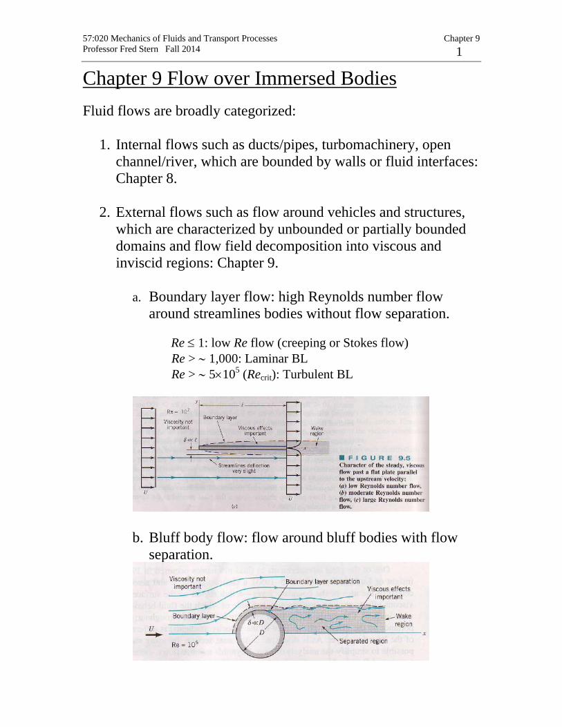
2. External flows such as flow around vehicles and structures, which are characterized by unbounded or partially bounded domains and flow field decomposition into viscous and inviscid regions: Chapter 9.
a. Boundary layer flow: high Reynolds number flow around streamlines bodies without flow separation. Re ≤ 1: low Re flow (creeping or Stokes flow) Re > ∼ 1,000: Laminar BL Re > ∼ 5×10⁵ (Recrit): Turbulent BL
b. Bluff body flow: flow around bluff bodies with flow separation.
57:020 Mechanics of Fluids and Transport Processes Chapter 9 Professor Fred Stern Fall 2014 2
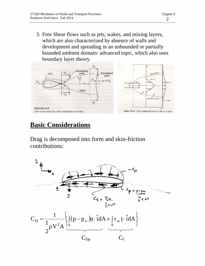
3. Free Shear flows such as jets, wakes, and mixing layers,
which are also characterized by absence of walls and development and spreading in an unbounded or partially bounded ambient domain: advanced topic, which also uses boundary layer theory.
Basic Considerations Drag is decomposed into form and skin-friction contributions:
( )
∫ ⋅τ+∫ ⋅−ρ
= ∞S
wS2
D dAitdAinppAV
21
1C
CDp Cf

57:020 Mechanics of Fluids and Transport Processes Chapter 9 Professor Fred Stern Fall 2014 3
( )
⋅∫ −
ρ= ∞ dAjnpp
AV21
1CS2
L
ct << 1 Cf > > CDp streamlined body
ct ∼ 1 CDp > > Cf bluff body
Streamlining: One way to reduce the drag reduce the flow separationreduce the pressure drag increase the surface area increase the friction drag Trade-off relationship between pressure drag and friction drag
Trade-off relationship between pressure drag and friction drag
Benefit of streamlining: reducing vibration and noise
57:020 Mechanics of Fluids and Transport Processes Chapter 9 Professor Fred Stern Fall 2014 4
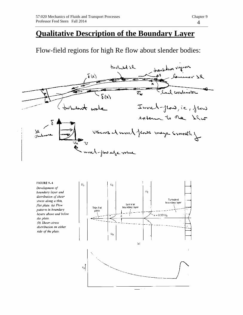
Qualitative Description of the Boundary Layer Flow-field regions for high Re flow about slender bodies:

57:020 Mechanics of Fluids and Transport Processes Chapter 9 Professor Fred Stern Fall 2014 5
τw = shear stress τw ∝ rate of strain (velocity gradient)
=0yy
u
=∂∂
µ
large near the surface where
fluid undergoes large changes to satisfy the no-slip condition
Boundary layer theory and equations are a simplified form of the complete NS equations and provides τw as well as a means of estimating Cform. Formally, boundary-layer theory represents the asymptotic form of the Navier-Stokes equations for high Re flow about slender bodies. The NS equations are 2nd order nonlinear PDE and their solutions represent a formidable challenge. Thus, simplified forms have proven to be very useful. Near the turn of the last century (1904), Prandtl put forth boundary-layer theory, which resolved D’Alembert’s paradox: for inviscid flow drag is zero. The theory is restricted to unseparated flow. The boundary-layer equations are singular at separation, and thus, provide no information at or beyond separation. However, the requirements of the theory are met in many practical situations and the theory has many times over proven to be invaluable to modern engineering.

57:020 Mechanics of Fluids and Transport Processes Chapter 9 Professor Fred Stern Fall 2014 6
The assumptions of the theory are as follows: Variable order of magnitude u U O(1) v δ<<L O(ε) ε = δ/L
x∂∂ 1/L O(1)
y∂∂ 1/δ O(ε-1)
ν δ2 ε2 The theory assumes that viscous effects are confined to a thin layer close to the surface within which there is a dominant flow direction (x) such that u ∼ U and v << u. However, gradients across δ are very large in order to
satisfy the no slip condition; thus, y∂∂ >>
x∂∂ .
Next, we apply the above order of magnitude estimates to the NS equations.

57:020 Mechanics of Fluids and Transport Processes Chapter 9 Professor Fred Stern Fall 2014 7
2 2
2 2
u u p u uu vx y x x y
ν ∂ ∂ ∂ ∂ ∂
+ = − + + ∂ ∂ ∂ ∂ ∂
1 1 ε ε-1 ε2 1 ε-2
2 2
2 2
v v p v vu vx y y x y
ν ∂ ∂ ∂ ∂ ∂
+ = − + + ∂ ∂ ∂ ∂ ∂
1 ε ε 1 ε2 ε ε-1
0yv
xu
=∂∂
+∂∂
1 1
Retaining terms of O(1) only results in the celebrated boundary-layer equations
2
2
u u p uu vx y x y
ν∂ ∂ ∂ ∂+ = − +
∂ ∂ ∂ ∂
0yp=
∂∂
0yv
xu
=∂∂
+∂∂
elliptic
parabolic

57:020 Mechanics of Fluids and Transport Processes Chapter 9 Professor Fred Stern Fall 2014 8
Some important aspects of the boundary-layer equations:
1) the y-momentum equation reduces to
0yp=
∂∂
i.e., p = pe = constant across the boundary layer
from the Bernoulli equation:
=ρ+ 2ee U
21p constant
i.e., x
UUxp e
ee
∂∂
ρ−=∂∂
Thus, the boundary-layer equations are solved subject to a specified inviscid pressure distribution
2) continuity equation is unaffected 3) Although NS equations are fully elliptic, the
boundary-layer equations are parabolic and can be solved using marching techniques
4) Boundary conditions
u = v = 0 y = 0 u = Ue y = δ
+ appropriate initial conditions @ xi
edge value, i.e., inviscid flow value!

57:020 Mechanics of Fluids and Transport Processes Chapter 9 Professor Fred Stern Fall 2014 9
There are quite a few analytic solutions to the boundary-layer equations. Also numerical techniques are available for arbitrary geometries, including both two- and three-dimensional flows. Here, as an example, we consider the simple, but extremely important case of the boundary layer development over a flat plate. Quantitative Relations for the Laminar Boundary Layer Laminar boundary-layer over a flat plate: Blasius solution (1908) student of Prandtl
0yv
xu
=∂∂
+∂∂
2
2
yu
yuv
xuu
∂∂
ν=∂∂
+∂∂
u = v = 0 @ y = 0 u = U∞ @ y = δ We now introduce a dimensionless transverse coordinate and a stream function, i.e.,
δ
∝ν
=η ∞ yx
Uy
( )ην=ψ ∞ fxU
Note: xp∂
∂ = 0
for a flat plate

57:020 Mechanics of Fluids and Transport Processes Chapter 9 Professor Fred Stern Fall 2014 10
( )η′=∂η∂
η∂ψ∂
=∂ψ∂
= ∞fUyy
u ∞=′ U/uf
( )ffxU
21
xv −′η
ν=
∂ψ∂
−= ∞
Substitution into the boundary-layer equations yields 0f2ff =′′′+′′ Blasius Equation 0ff =′= @ η = 0 1f =′ @ η → ∞ The Blasius equation is a 3rd order ODE which can be solved by standard methods (Runge-Kutta). Also, series solutions are possible. Interestingly, although simple in appearance no analytic solution has yet been found. Finally, it should be recognized that the Blasius solution is a similarity solution, i.e., the non-dimensional velocity profile f′ vs. η is independent of x. That is, by suitably scaling all the velocity profiles have neatly collapsed onto a single curve. Now, lets consider the characteristics of the Blasius solution:
∞U
u vs. y
∞Uv
vs. y

57:020 Mechanics of Fluids and Transport Processes Chapter 9 Professor Fred Stern Fall 2014 11
5Rex
xδ = value of y where u/U∞ = .99
RexU xν∞=

57:020 Mechanics of Fluids and Transport Processes Chapter 9 Professor Fred Stern Fall 2014 12
∞ν
′′∞µ=τ
U/x2
)0(fUw
see below
i.e., xRe
664.0U
2cx
2w
fθ
==ρτ
=∞
: Local friction coeff.
∫ ==L
fff LcdxcbLbC
0
)(2 : Friction drag coeff.
=LRe
328.1 ν∞LU
Wall shear stress: 3 20.332w Uxρµτ ∞= or ( )0.332 Rew xU xτ µ ∞=
Other:
∫ =
−=δ
δ
∞0 x
*
Rex7208.1dy
Uu1 displacement thickness
measure of displacement of inviscid flow due to boundary layer
∫ =
−=θ
δ
∞∞0 xRex664.0dy
Uu
Uu1 momentum thickness
measure of loss of momentum due to boundary layer
H = shape parameter = θδ*
=2.5916
Note: 𝑏𝑏 = plate width 𝐿𝐿 = plate length
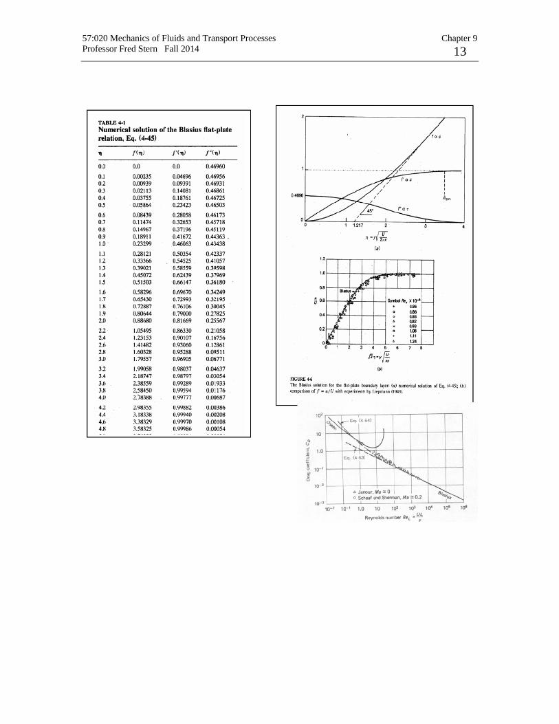
57:020 Mechanics of Fluids and Transport Processes Chapter 9 Professor Fred Stern Fall 2014 13
57:020 Mechanics of Fluids and Transport Processes Chapter 9 Professor Fred Stern Fall 2014 14
For flat plate or δ for general case
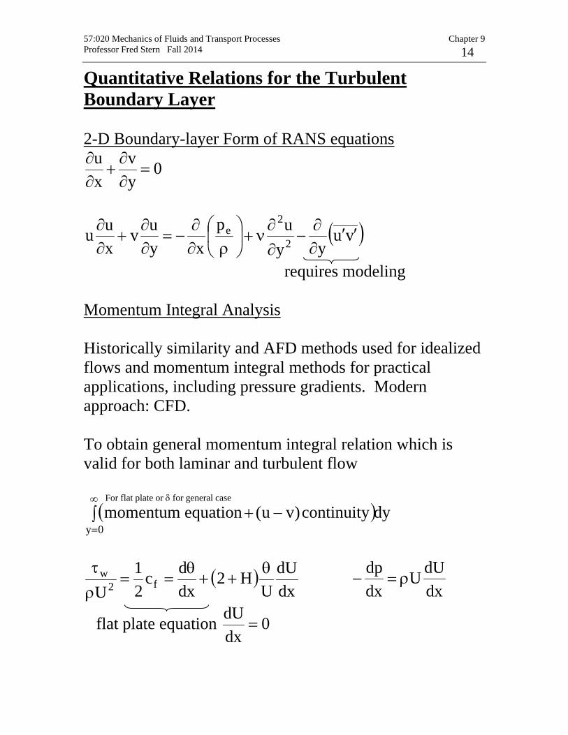
Quantitative Relations for the Turbulent Boundary Layer 2-D Boundary-layer Form of RANS equations
0yv
xu
=∂∂
+∂∂
( )vuyy
upxy
uvxuu 2
2e ′′
∂∂
−∂∂
ν+
ρ∂
∂−=
∂∂
+∂∂
requires modeling Momentum Integral Analysis Historically similarity and AFD methods used for idealized flows and momentum integral methods for practical applications, including pressure gradients. Modern approach: CFD. To obtain general momentum integral relation which is valid for both laminar and turbulent flow
( )dycontinuity)vu(equationmomentum0y∫ −+∞
=
( )dxdU
UH2
dxdc
21
U f2w θ
++θ
==ρτ
dxdUU
dxdp
ρ=−
flat plate equation 0dxdU
=

57:020 Mechanics of Fluids and Transport Processes Chapter 9 Professor Fred Stern Fall 2014 15
∫
−=θ
δ
0dy
Uu1
Uu momentum thickness
θδ
=*
H shape parameter
dyUu1
0
* ∫
−=δ
δ displacement thickness
Can also be derived by CV analysis as shown next for flat plate boundary layer. Momentum Equation Applied to the Boundary Layer Consider flow of a viscous fluid at high Re past a flat plate, i.e., flat plate fixed in a uniform stream of velocity ˆUi . Boundary-layer thickness arbitrarily defined by y = %99δ (where,
%99δ is the value of y at u = 0.99U). Streamlines outside %99δ will deflect an amount *δ (the displacement thickness). Thus the streamlines move outward from Hy = at 0=x to
*δδ +=== HYy at 1xx = .

57:020 Mechanics of Fluids and Transport Processes Chapter 9 Professor Fred Stern Fall 2014 16
Conservation of mass:
CS
V ndAρ •∫ =0= 0 0
H HUdy udy
δρ ρ
∗+− +∫ ∫
Assume incompressible flow (constant density):
( ) ( )∫ ∫ ∫ −+=−+==Y Y Y
dyUuUYdyUuUudyUH0 0 0
Substituting *δ+= HY defines displacement thickness:
dyUuY
∫
−= 0
* 1δ
*δ is an important measure of effect of BL on external flow. Consider alternate derivation based on equivalent flow rate:
∫∫ =δδ
δ 0*
udyUdy
Flowrate between *δ and δ of inviscid flow=actual flowrate, i.e., inviscid flow rate about displacement body = viscous flow rate about actual body
∫∫∫∫
−=⇒=−
δδδδ
δ0
*
000
1*
dyUuudyUdyUdy
w/o BL - displacement effect=actual discharge
For 3D flow, in addition it must also be explicitly required that *δis a stream surface of the inviscid flow continued from outside of the BL.
δ* Lam=δ/3
δ
δ* Turb=δ/8
Inviscid flow about δ* body

57:020 Mechanics of Fluids and Transport Processes Chapter 9 Professor Fred Stern Fall 2014 17
Conservation of x-momentum: ( ) ( )
0 0
H Y
xCS
F D uV ndA U Udy u udyρ ρ ρ= − = • = − +∑ ∫ ∫ ∫
dyuHUDDrag Y∫−== 0
22 ρρ = Fluid force on plate = - Plate force on CV (fluid) Again assuming constant density and using continuity:
∫=Y
dyUuH
0
2 2
0 00
/Y
Y x
wD U u Udy u dy dxρ ρ τ= − =∫ ∫ ∫
dyUu
Uu
UD Y
−== ∫ 102 θ
ρ
where, θ is the momentum thickness (a function of x only), an important measure of the drag.
20
2 2 1 x
D fDC c dx
U x x xθ
ρ= = = ∫
( )2
212
wf f D
d dc c xCdx dxU
τ θ
ρ= ⇒ = =
2fcd
dxθ= dx
dUwθρτ 2=
Per unit span
Special case 2D momentum integral equation for dp/dx = 0
57:020 Mechanics of Fluids and Transport Processes Chapter 9 Professor Fred Stern Fall 2014 18
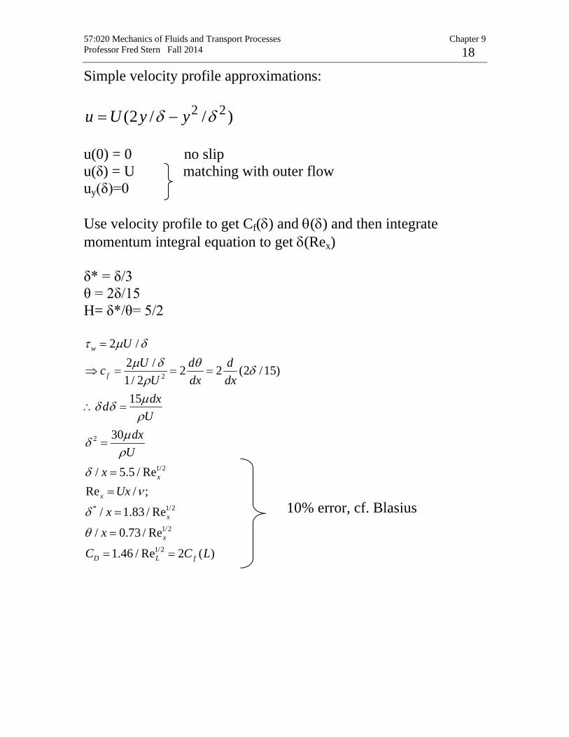
Simple velocity profile approximations:
)//2( 22 δδ yyUu −= u(0) = 0 no slip u(δ) = U matching with outer flow uy(δ)=0 Use velocity profile to get Cf(δ) and θ(δ) and then integrate momentum integral equation to get δ(Rex) δ* = δ/3 θ = 2δ/15 H= δ*/θ= 5/2
2
2
1/2
* 1/2
1/2
1/2
2 /2 / 2 2 (2 /15)1/ 215
30
/ 5.5 / ReRe / ;
/ 1.83 / Re
/ 0.73 / Re
1.46 / Re 2 ( )
w
f
x
x
x
x
D L f
UU d dc
U dx dxdxd
Udx
Ux
Ux
x
x
C C L
τ µ δµ δ θ δρµδ δρ
µδρ
δν
δ
θ
=
⇒ = = =
∴ =
=
=
=
=
=
= =
10% error, cf. Blasius
57:020 Mechanics of Fluids and Transport Processes Chapter 9 Professor Fred Stern Fall 2014 19
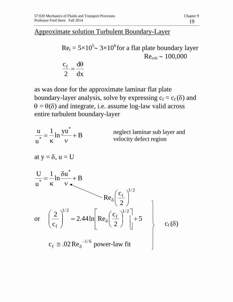
Approximate solution Turbulent Boundary-Layer Ret = 5×10⁵∼ 3×10⁶ for a flat plate boundary layer Recrit ∼ 100,000
dxd
2cf θ
=
as was done for the approximate laminar flat plate boundary-layer analysis, solve by expressing cf = cf (δ) and θ = θ(δ) and integrate, i.e. assume log-law valid across entire turbulent boundary-layer
Byuln1uu *
* +νκ
=
at y = δ, u = U
Buln1uU *
* +νδ
κ=
2/1
f
2cRe
δ
or 52cReln44.2
c2 2/1
f2/1
f+
=
δ
6/1
f Re02.c −δ≅ power-law fit
neglect laminar sub layer and velocity defect region
cf (δ)

57:020 Mechanics of Fluids and Transport Processes Chapter 9 Professor Fred Stern Fall 2014 20
Next, evaluate
∫
−=
θ δ
0dy
Uu1
Uu
dxd
dxd
can use log-law or more simply a power law fit
7/1yUu
δ
=
( )δθ=δ=θ727
⇒ dxdU
727
dxdUU
21c 222
fwδ
ρ=θ
ρ=ρ=τ
dxd72.9Re 6/1 δ
=−δ
or 1/70.16Rexxδ −=
7/6x∝δ almost linear
1/7
0.027Ref
x
c =
( )1/7
0.031 7Re 6f f
L
C c L= =
These formulas are for a fully turbulent flow over a smooth flat plate from the leading edge; in general, give better results for sufficiently large Reynolds number ReL > 107.
Note: cannot be used to obtain cf (δ) since τw → ∞
i.e., much faster growth rate than laminar boundary layer

57:020 Mechanics of Fluids and Transport Processes Chapter 9 Professor Fred Stern Fall 2014 21
Comparison of dimensionless laminar and turbulent flat-plate velocity profiles (Ref:
White, F. M., Fluid Mechanics, 7th Ed., McGraw-Hill)
Alternate forms by using the same velocity profile u/U = (y/δ)1/7 assumption but using an experimentally determined shear stress formula τw = 0.0225ρU2(ν/Uδ)1/4 are:
1/50.37 Rexxδ −= 1/5
0.058Ref
x
c = 1/5
0.074Ref
L
C =
shear stress: 2
1/5
0.029Rew
x
Uρτ =
These formulas are valid only in the range of the experimental data, which covers ReL = 5 × 10⁵ ∼ 107 for smooth flat plates. Other empirical formulas are by using the logarithmic velocity-profile instead of the 1/7-power law:
𝑢𝑢𝑈𝑈≈ �
𝑦𝑦𝛿𝛿�17
𝑢𝑢𝑈𝑈≈ 2 �
𝑦𝑦𝛿𝛿� − �
𝑦𝑦𝛿𝛿�2
(See Table 4-1 on page 13 of this lecture note)

57:020 Mechanics of Fluids and Transport Processes Chapter 9 Professor Fred Stern Fall 2014 22
𝛿𝛿
𝐿𝐿= 𝑐𝑐𝑓𝑓(0.98 log𝑅𝑅𝑅𝑅𝐿𝐿 − 0.732)
𝑐𝑐𝑓𝑓 = (2 log𝑅𝑅𝑅𝑅𝑥𝑥 − 0.65)−2.3 𝐶𝐶𝑓𝑓 = 0.455
(log10 𝑅𝑅𝑒𝑒𝐿𝐿)2.58
These formulas are also called as the Prandtl-Schlichting skin-friction formula and valid in the whole range of ReL ≤ 109. For these experimental/empirical formulas, the boundary layer is usually “tripped” by some roughness or leading edge disturbance, to make the boundary layer turbulent from the leading edge. No definitive values for turbulent conditions since depend on empirical data and turbulence modeling. Finally, composite formulas that take into account both the initial laminar boundary layer and subsequent turbulent boundary layer, i.e. in the transition region (5 × 10⁵ < ReL < 8 × 10⁷) where the laminar drag at the leading edge is an appreciable fraction of the total drag:
𝐶𝐶𝑓𝑓 =0.031
𝑅𝑅𝑅𝑅𝐿𝐿17−
1440𝑅𝑅𝑅𝑅𝐿𝐿
𝐶𝐶𝑓𝑓 =
0.074
𝑅𝑅𝑅𝑅𝐿𝐿15−
1700𝑅𝑅𝑅𝑅𝐿𝐿

57:020 Mechanics of Fluids and Transport Processes Chapter 9 Professor Fred Stern Fall 2014 23
𝐶𝐶𝑓𝑓 =0.455
(log10 𝑅𝑅𝑅𝑅𝐿𝐿)2.58 −1700𝑅𝑅𝑅𝑅𝐿𝐿
with transitions at Ret = 5 × 10⁵ for all cases.
Local friction coefficient 𝑐𝑐𝑓𝑓 (top) and friction drag coefficient 𝐶𝐶𝑓𝑓(bottom) for a flat plate parallel to the upstream flow.
57:020 Mechanics of Fluids and Transport Processes Chapter 9 Professor Fred Stern Fall 2014 24
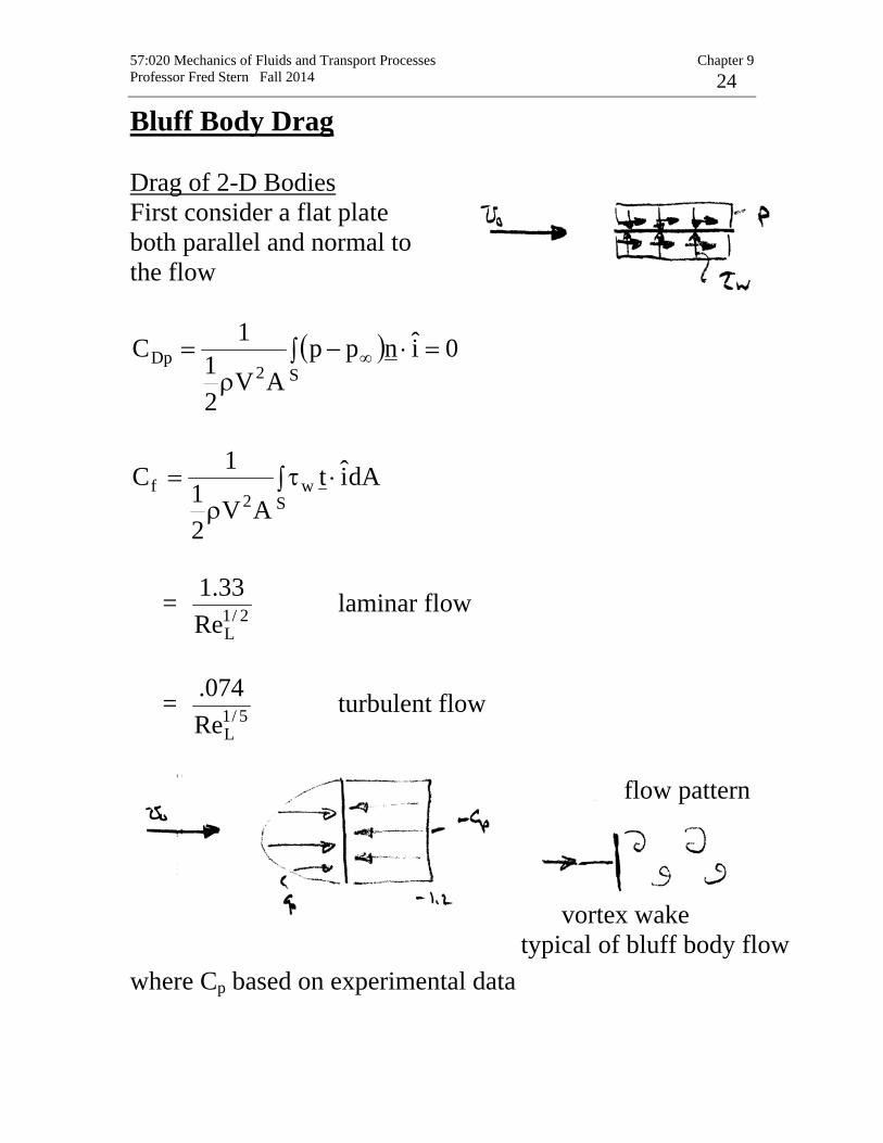
Bluff Body Drag Drag of 2-D Bodies First consider a flat plate both parallel and normal to the flow
( ) 0inppAV
21
1CS2
Dp =∫ ⋅−ρ
= ∞
∫ ⋅τρ
=S
w2
f dAitAV
21
1C
= 2/1LRe33.1 laminar flow
= 5/1LRe
074. turbulent flow
where Cp based on experimental data
vortex wake typical of bluff body flow
flow pattern

57:020 Mechanics of Fluids and Transport Processes Chapter 9 Professor Fred Stern Fall 2014 25
( )∫ ⋅−
ρ= ∞
S2Dp dAinpp
AV21
1C
= ∫S
pdACA1
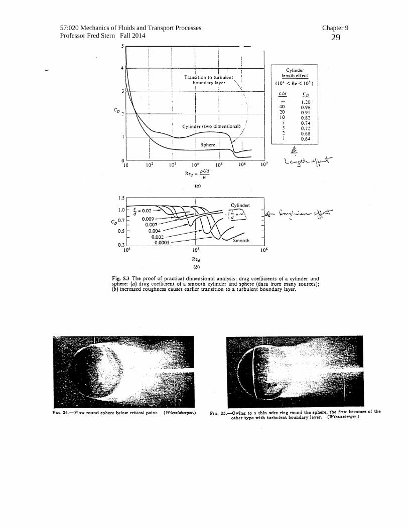
= 2 using numerical integration of experimental data Cf = 0 For bluff body flow experimental data used for CD.
57:020 Mechanics of Fluids and Transport Processes Chapter 9 Professor Fred Stern Fall 2014 26
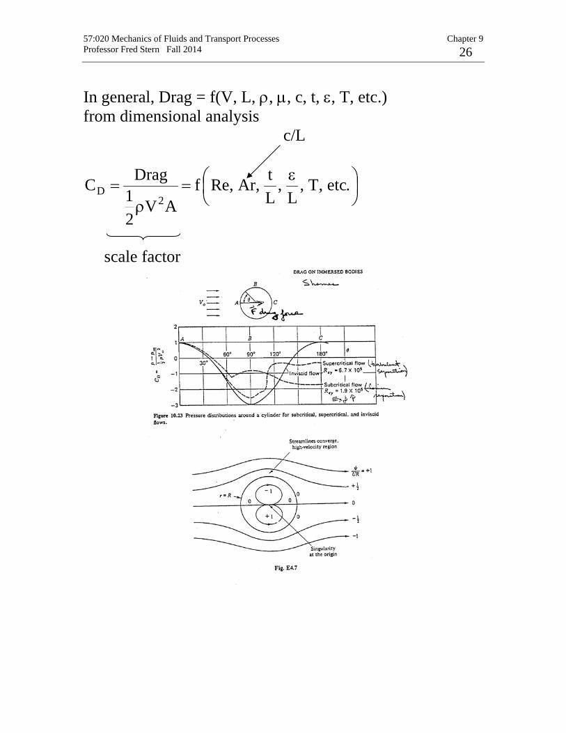
In general, Drag = f(V, L, ρ, µ, c, t, ε, T, etc.) from dimensional analysis c/L
ε
=ρ
= .etc,T,L
,Lt,ArRe,f
AV21
DragC2
D
scale factor

57:020 Mechanics of Fluids and Transport Processes Chapter 9 Professor Fred Stern Fall 2014 27
Potential Flow Solution: θ
−−=ψ ∞ sin
rarU
2
22 U21pV
21p ∞∞ ρ+=ρ+
2
22r
2p U
uu1U
21
ppC∞
θ
∞
∞ +−=
ρ
−=
( ) θ−== 2p sin41arC surface pressure
Flow Separation Flow separation: The fluid stream detaches itself from the surface of the body at sufficiently high velocities. Only appeared in viscous flow!! Flow separation forms the region called ‘separated region’
ru
r1ur
∂ψ∂
−=
θ∂ψ∂
=
θ

57:020 Mechanics of Fluids and Transport Processes Chapter 9 Professor Fred Stern Fall 2014 28
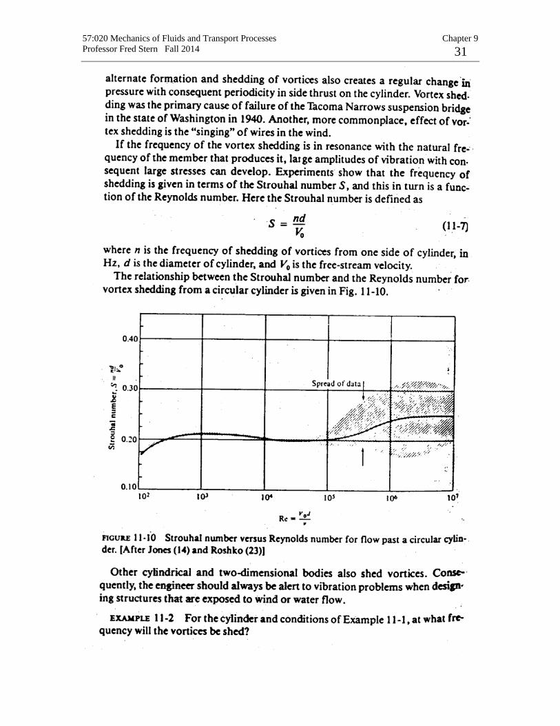
Inside the separation region: low-pressure, existence of recirculating/backflows viscous and rotational effects are the most significant! Important physics related to flow separation: ’Stall’ for airplane (Recall the movie you saw at CFD-PreLab2!) Vortex shedding (Recall your work at CFD-Lab2, AOA=16°! What did you see in your velocity-vector plot at the trailing edge of the air foil?)
57:020 Mechanics of Fluids and Transport Processes Chapter 9 Professor Fred Stern Fall 2014 29

57:020 Mechanics of Fluids and Transport Processes Chapter 9 Professor Fred Stern Fall 2014 30
57:020 Mechanics of Fluids and Transport Processes Chapter 9 Professor Fred Stern Fall 2014 31

57:020 Mechanics of Fluids and Transport Processes Chapter 9 Professor Fred Stern Fall 2014 32

57:020 Mechanics of Fluids and Transport Processes Chapter 9 Professor Fred Stern Fall 2014 33

57:020 Mechanics of Fluids and Transport Processes Chapter 9 Professor Fred Stern Fall 2014 34
57:020 Mechanics of Fluids and Transport Processes Chapter 9 Professor Fred Stern Fall 2014 35

57:020 Mechanics of Fluids and Transport Processes Chapter 9 Professor Fred Stern Fall 2014 36

57:020 Mechanics of Fluids and Transport Processes Chapter 9 Professor Fred Stern Fall 2014 37
57:020 Mechanics of Fluids and Transport Processes Chapter 9 Professor Fred Stern Fall 2014 38
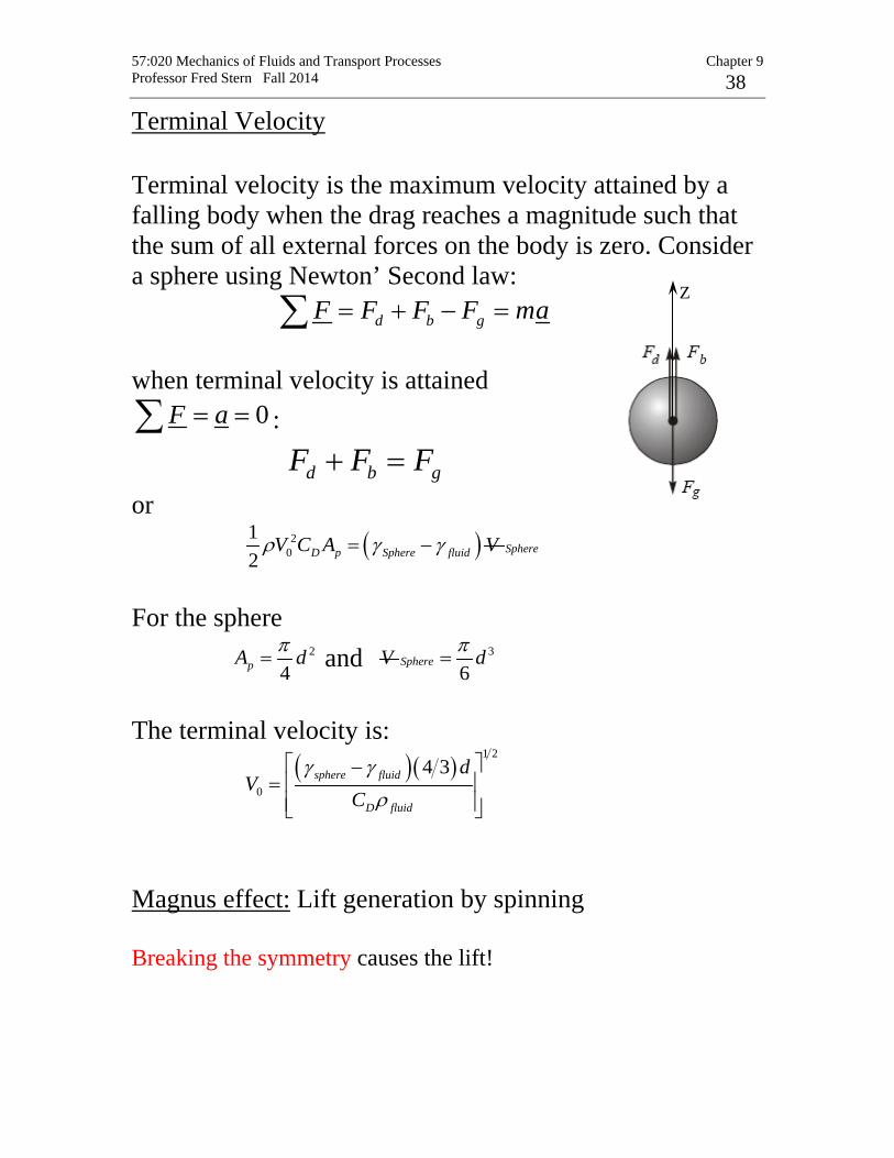
Terminal Velocity Terminal velocity is the maximum velocity attained by a falling body when the drag reaches a magnitude such that the sum of all external forces on the body is zero. Consider a sphere using Newton’ Second law: d b gF F F F ma= + − =∑ when terminal velocity is attained
0F a= =∑ :
d b gF F F+ = or ( )2
012 D p Sphere fluidV C A Vρ γ γ= − Sphere
For the sphere 2
4pA dp= and V 3
6Sphere dp
= The terminal velocity is:
( )( )
1 2
0
4 3sphere fluid
D fluid
dV
Cγ γ
ρ
−=
Magnus effect: Lift generation by spinning Breaking the symmetry causes the lift!
Z
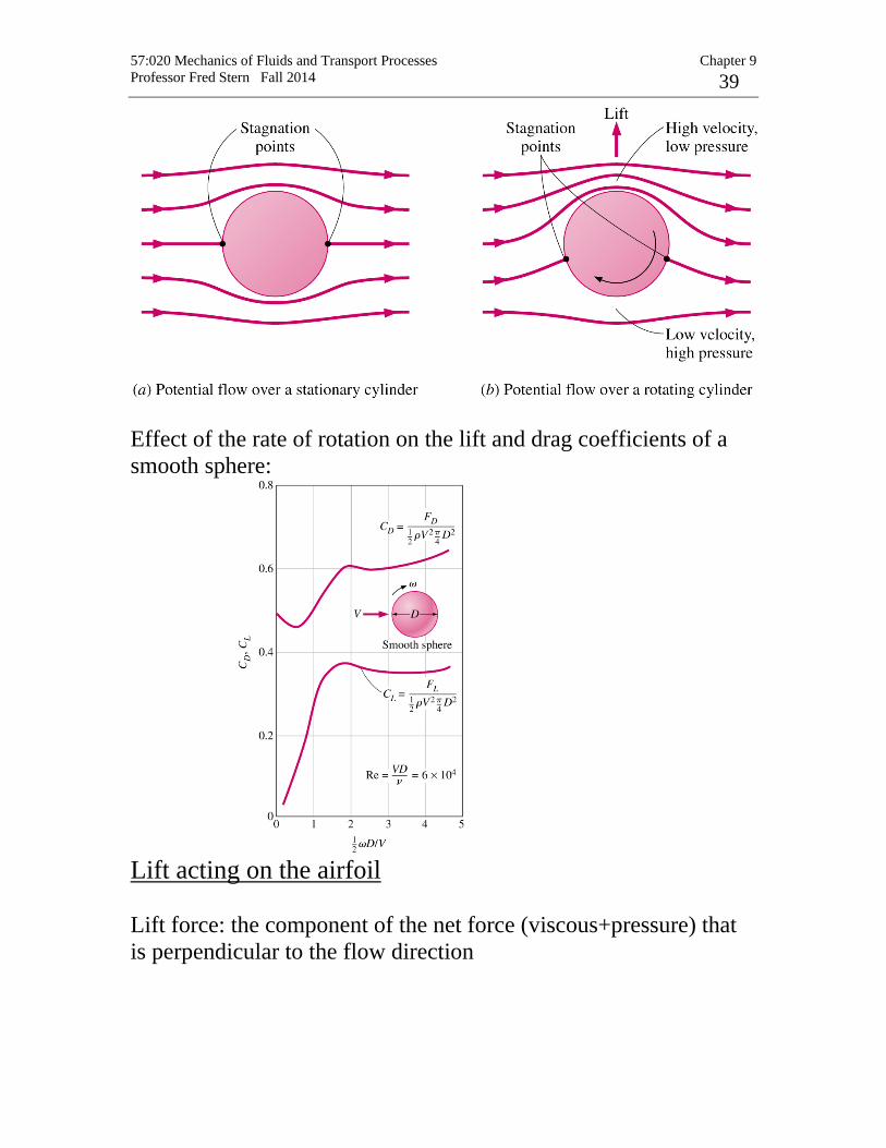
57:020 Mechanics of Fluids and Transport Processes Chapter 9 Professor Fred Stern Fall 2014 39
Effect of the rate of rotation on the lift and drag coefficients of a smooth sphere:
Lift acting on the airfoil Lift force: the component of the net force (viscous+pressure) that is perpendicular to the flow direction

57:020 Mechanics of Fluids and Transport Processes Chapter 9 Professor Fred Stern Fall 2014 40
Variation of the lift-to-drag ratio with angle of attack:
The minimum flight velocity: Total weight W of the aircraft be equal to the lift
ACWVAVCFW
LLL
max,min
2minmax,
221
ρρ =→==

57:020 Mechanics of Fluids and Transport Processes Chapter 9 Professor Fred Stern Fall 2014 41
< 0.3 flow is incompressible, i.e., ρ ∼ constant
Effect of Compressibility on Drag: CD = CD(Re, Ma)
aUMa ∞=
speed of sound = rate at which infinitesimal disturbances are propagated from their source into undisturbed medium
Ma < 1 subsonic Ma ∼ 1 transonic (=1 sonic flow) Ma > 1 supersonic Ma >> 1 hypersonic CD increases for Ma ∼ 1 due to shock waves and wave drag
Macritical(sphere) ∼ .6 Macritical(slender bodies) ∼ 1 For U > a: upstream flow is not warned of approaching
disturbance which results in the formation of shock waves across which flow properties and streamlines change discontinuously

57:020 Mechanics of Fluids and Transport Processes Chapter 9 Professor Fred Stern Fall 2014 42