Professional Edition, Version...
102
Agisoft PhotoScan User Manual Professional Edition, Version 1.2
Transcript of Professional Edition, Version...

Agisoft PhotoScan User Manual
Professional Edition, Version 1.2

Agisoft PhotoScan User Manual: Professional Edition, Version 1.2
Publication date 2016Copyright © 2016 Agisoft LLC
iii
Table of ContentsOverview .......................................................................................................................... v
How it works ............................................................................................................. vAbout the manual ....................................................................................................... v
1. Installation ..................................................................................................................... 1System requirements ................................................................................................... 1OpenCL acceleration ................................................................................................... 1Installation procedure .................................................................................................. 2Restrictions of the Demo mode ..................................................................................... 2
2. Capturing photos ............................................................................................................ 4Equipment ................................................................................................................. 4Camera settings .......................................................................................................... 4Object/scene requirements ............................................................................................ 4Image preprocessing ................................................................................................... 4Capturing scenarios ..................................................................................................... 5Restrictions ............................................................................................................... 6
3. General workflow ........................................................................................................... 8Preferences settings ..................................................................................................... 8Loading photos .......................................................................................................... 8Aligning photos ........................................................................................................ 11Building dense point cloud ......................................................................................... 14Building mesh .......................................................................................................... 15Building model texture .............................................................................................. 17Building tiled model .................................................................................................. 19Building digital elevation model .................................................................................. 20Building orthomosaic ................................................................................................. 21Saving intermediate results ......................................................................................... 22Exporting results ....................................................................................................... 23
4. Referencing .................................................................................................................. 35Camera calibration .................................................................................................... 35Setting coordinate system ........................................................................................... 37Optimization ............................................................................................................ 43Working with coded and non-coded targets ................................................................... 46
5. Measurements ............................................................................................................... 48Performing measurements on mesh .............................................................................. 48Performing measurements on DEM .............................................................................. 49Vegetation indices calculation ..................................................................................... 51
6. Editing ........................................................................................................................ 53Using masks ............................................................................................................ 53Editing point cloud ................................................................................................... 57Classifying dense cloud points .................................................................................... 59Editing model geometry ............................................................................................. 61Orthomosaic seamlines editing .................................................................................... 64
7. Automation .................................................................................................................. 66Using chunks ........................................................................................................... 664D processing .......................................................................................................... 70Python scripting ........................................................................................................ 72
8. Network processing ....................................................................................................... 73Overview ................................................................................................................. 73Cluster components ................................................................................................... 73Cluster setup ............................................................................................................ 74Cluster administration ................................................................................................ 76
Agisoft PhotoScan User Manual
iv
A. Graphical user interface ................................................................................................. 77Application window .................................................................................................. 77Menu commands ...................................................................................................... 81Toolbar buttons ........................................................................................................ 86Hot keys ................................................................................................................. 88
B. Supported formats ......................................................................................................... 91Images .................................................................................................................... 91Camera calibration .................................................................................................... 91Camera flight log ...................................................................................................... 91GCP locations .......................................................................................................... 91Interior and exterior camera orientation parameters ......................................................... 92Tie points ................................................................................................................ 92Sparse/dense point cloud ............................................................................................ 92Mesh model ............................................................................................................. 92Texture ................................................................................................................... 93Orthomosaic ............................................................................................................. 93Digital elevation model (DSM/DTM) ........................................................................... 93Tiled models ............................................................................................................ 94Shapes and contours .................................................................................................. 94
C. Camera models ............................................................................................................ 95Frame cameras ......................................................................................................... 95Fisheye cameras ....................................................................................................... 95Spherical cameras (equirectangular projection) ............................................................... 96Spherical cameras (cylindrical projection) ..................................................................... 96
v
OverviewAgisoft PhotoScan is an advanced image-based 3D modeling solution aimed at creating professionalquality 3D content from still images. Based on the latest multi-view 3D reconstruction technology, itoperates with arbitrary images and is efficient in both controlled and uncontrolled conditions. Photos canbe taken from any position, providing that the object to be reconstructed is visible on at least two photos.Both image alignment and 3D model reconstruction are fully automated.
How it worksGenerally the final goal of photographs processing with PhotoScan is to build a textured 3D model. Theprocedure of photographs processing and 3D model construction comprises four main stages.
1. The first stage is camera alignment. At this stage PhotoScan searches for common points on photographsand matches them, as well as it finds the position of the camera for each picture and refines cameracalibration parameters. As a result a sparse point cloud and a set of camera positions are formed.
The sparse point cloud represents the results of photo alignment and will not be directly used inthe further 3D model construction procedure (except for the sparse point cloud based reconstructionmethod). However it can be exported for further usage in external programs. For instance, the sparsepoint cloud model can be used in a 3D editor as a reference.
On the contrary, the set of camera positions is required for further 3D model reconstruction byPhotoScan.
2. The next stage is building dense point cloud. Based on the estimated camera positions and picturesthemselves a dense point cloud is built by PhotoScan. Dense point cloud may be edited and classifiedprior to export or proceeding to 3D mesh model generation.
3. The third stage is building mesh. PhotoScan reconstructs a 3D polygonal mesh representing the objectsurface based on the dense or sparse point cloud according to the user's choice. Generally there are twoalgorithmic methods available in PhotoScan that can be applied to 3D mesh generation: Height Field- for planar type surfaces, Arbitrary - for any kind of object.
The mesh having been built, it may be necessary to edit it. Some corrections, such as mesh decimation,removal of detached components, closing of holes in the mesh, smoothing, etc. can be performed byPhotoScan. For more complex editing you have to engage external 3D editor tools. PhotoScan allowsto export mesh, edit it by another software and import it back.
4. After geometry (i.e. mesh) is reconstructed, it can be textured and/or used for orthomosaic generation.Several texturing modes are available in PhotoScan, they are described in the corresponding section ofthis manual, as well as orthomosaic and DEM generation procedures.
About the manualBasically, the sequence of actions described above covers most of the data processing needs. All theseoperations are carried out automatically according to the parameters set by user. Instructions on how toget through these operations and descriptions of the parameters controlling each step are given in thecorresponding sections of the Chapter 3, General workflow chapter of the manual.
In some cases, however, additional actions may be required to get the desired results. In some capturingscenarios masking of certain regions of the photos may be required to exclude them from the calculations.Application of masks in PhotoScan processing workflow as well as editing options available are described
Overview
vi
in Chapter 6, Editing. Camera calibration issues are discussed in Chapter 4, Referencing, that alsodescribes functionality to optimize camera alignment results and provides guidance on model referencing.A referenced model, be it a mesh or a DEM serves as a ground for measurements. Area, volume, profilemeasurement procedures are tackled in Chapter 5, Measurements, which also includes information onvegetation indices calculations. While Chapter 7, Automation describes opportunities to save up on manualintervention to the processing workflow, Chapter 8, Network processing presents guidelines on how toorganize distributed processing of the imagery data on several nodes.
It can take up quite a long time to reconstruct a 3D model. PhotoScan allows to export obtained resultsand save intermediate data in a form of project files at any stage of the process. If you are not familiar withthe concept of projects, its brief description is given at the end of the Chapter 3, General workflow.
In the manual you can also find instructions on the PhotoScan installation procedure and basic rules fortaking "good" photographs, i.e. pictures that provide most necessary information for 3D reconstruction.For the information refer to Chapter 1, Installation and Chapter 2, Capturing photos.

1
Chapter 1. InstallationSystem requirements
Minimal configuration
• Windows XP or later (32 or 64 bit), Mac OS X Snow Leopard or later, Debian/Ubuntu (64 bit)
• Intel Core 2 Duo processor or equivalent
• 2GB of RAM
Recommended configuration
• Windows XP or later (64 bit), Mac OS X Snow Leopard or later, Debian/Ubuntu (64 bit)
• Intel Core i7 processor
• 12GB of RAM
The number of photos that can be processed by PhotoScan depends on the available RAM andreconstruction parameters used. Assuming that a single photo resolution is of the order of 10 MPix, 2GBRAM is sufficient to make a model based on 20 to 30 photos. 12GB RAM will allow to process up to200-300 photographs.
OpenCL accelerationPhotoScan supports accelerated depth maps reconstruction due to the graphics hardware (GPU) exploiting.
NVidiaGeForce 8xxx series and later.
ATIRadeon HD 5xxx series and later.
PhotoScan is likely to be able to utilize processing power of any OpenCL enabled device during DensePoint Cloud generation stage, provided that OpenCL drivers for the device are properly installed. However,because of the large number of various combinations of video chips, driver versions and operating systems,Agisoft is unable to test and guarantee PhotoScan's compatibility with every device and on every platform.
The table below lists currently supported devices (on Windows platform only). We will pay particularattention to possible problems with PhotoScan running on these devices.
Table 1.1. Supported Desktop GPUs on Windows platform
NVIDIA AMD
Quadro M6000 Radeon R9 290x
GeForce GTX TITAN Radeon HD 7970
GeForce GTX 980 Radeon HD 6970
GeForce GTX 780 Radeon HD 6950
GeForce GTX 680 Radeon HD 6870
Installation
2
NVIDIA AMD
GeForce GTX 580 Radeon HD 5870
GeForce GTX 570 Radeon HD 5850
GeForce GTX 560 Radeon HD 5830
GeForce GTX 480
GeForce GTX 470
GeForce GTX 465
GeForce GTX 285
GeForce GTX 280
Although PhotoScan is supposed to be able to utilize other GPU models and being run under a differentoperating system, Agisoft does not guarantee that it will work correctly.
Note
• OpenCL acceleration can be enabled using OpenCL tab in the Preferences dialog box. For eachOpenCL device used, one physical CPU core should be disabled for optimal performance.
• Using OpenCL acceleration with mobile or integrated graphics video chips is not recommendedbecause of the low performance of such GPUs.
Installation procedure
Installing PhotoScan on Microsoft WindowsTo install PhotoScan on Microsoft Windows simply run the downloaded msi file and follow theinstructions.
Installing PhotoScan on Mac OS XOpen the downloaded dmg image and drag PhotoScan application to the desired location on your harddrive.
Installing PhotoScan on Debian/UbuntuUnpack the downloaded archive with a program distribution kit to the desired location on your hard drive.Start PhotoScan by running photoscan.sh script from the program folder.
Restrictions of the Demo modeOnce PhotoScan is downloaded and installed on your computer you can run it either in the Demo modeor in the full function mode. On every start until you enter a serial number it will show a registrationbox offering two options: (1) use PhotoScan in the Demo mode or (2) enter a serial number to confirmthe purchase. The first choice is set by default, so if you are still exploring PhotoScan click the Continuebutton and PhotoScan will start in the Demo mode.
The employment of PhotoScan in the Demo mode is not time limited. Several functions, however, are notavailable in the Demo mode. These functions are the following:
Installation
3
• saving the project;
• build tiled model;
• build orthomosaic;
• build DEM;
• DEM and orthomosaic related features (such as Raster Calculator, DEM-based measurements);
• some Python commands.
• exporting reconstruction results (you can only view a 3D model on the screen);
To use PhotoScan in the full function mode you have to purchase it. On purchasing you will get the serialnumber to enter into the registration box on starting PhotoScan. Once the serial number is entered theregistration box will not appear again and you will get full access to all functions of the program.

4
Chapter 2. Capturing photosBefore loading your photographs into PhotoScan you need to take them and select those suitable for 3Dmodel reconstruction.
Photographs can be taken by any digital camera (both metric and non-metric), as long as you follow somespecific capturing guidelines. This section explains general principles of taking and selecting pictures thatprovide the most appropriate data for 3D model generation.
IMPORTANT! Make sure you have studied the following rules and read the list of restrictions before youget out for shooting photographs.
Equipment• Use a digital camera with reasonably high resolution (5 MPix or more).
• Avoid ultra-wide angle and fisheye lenses. The best choice is 50 mm focal length (35 mm filmequivalent) lenses. It is recommended to use focal length from 20 to 80 mm interval in 35mm equivalent.If a data set was captured with fisheye lens, appropriate camera sensor type should be selected inPhotoScan Camera Calibration dialog prior to processing.
• Fixed lenses are preferred. If zoom lenses are used - focal length should be set either to maximal or tominimal value during the entire shooting session for more stable results.
Camera settings• Using RAW data losslessly converted to the TIFF files is preferred, since JPG compression induces
unwanted noise to the images.
• Take images at maximal possible resolution.
• ISO should be set to the lowest value, otherwise high ISO values will induce additional noise to images.
• Aperture value should be high enough to result in sufficient focal depth: it is important to capture sharp,not blurred photos.
• Shutter speed should not be too slow, otherwise blur can occur due to slight movements.
Object/scene requirements• Avoid not textured, shiny, mirror or transparent objects.
• If still have to, shoot shiny objects under a cloudy sky.
• Avoid unwanted foregrounds.
• Avoid moving objects within the scene to be reconstructed.
• Avoid absolutely flat objects or scenes.
Image preprocessing• PhotoScan operates with the original images. So do not crop or geometrically transform, i.e. resize or
rotate, the images.
Capturing photos
5
Capturing scenariosGenerally, spending some time planning your shot session might be very useful.
• Number of photos: more than required is better than not enough.
• Number of "blind-zones" should be minimized since PhotoScan is able to reconstruct only geometryvisible from at least two cameras.
In case of aerial photography the overlap requirement can be put in the following figures: 60% of sideoverlap + 80% of forward overlap.
• Each photo should effectively use the frame size: object of interest should take up the maximum area.In some cases portrait camera orientation should be used.
• Do not try to place full object in the image frame, if some parts are missing it is not a problem providingthat these parts appear on other images.
• Good lighting is required to achieve better quality of the results, yet blinks should be avoided. It isrecommended to remove sources of light from camera fields of view. Avoid using flash.
• If you are planning to carry out any measurements based on the reconstructed model, do not forget tolocate at least two markers with a known distance between them on the object. Alternatively, you couldplace a ruler within the shooting area.
• In case of aerial photography and demand to fulfil georeferencing task, even spread of ground controlpoints (GCPs) (at least 10 across the area to be reconstructed) is required to achieve results of highestquality, both in terms of the geometrical precision and georeferencing accuracy. Yet, Agisoft PhotoScanis able to complete the reconstruction and georeferencing tasks without GCPs, too.
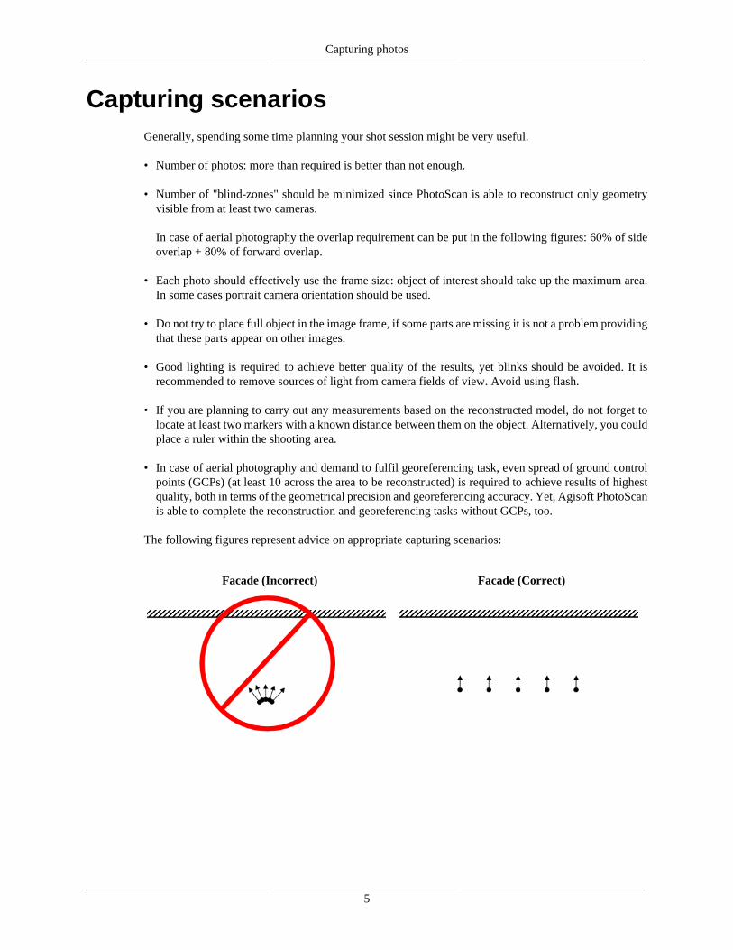
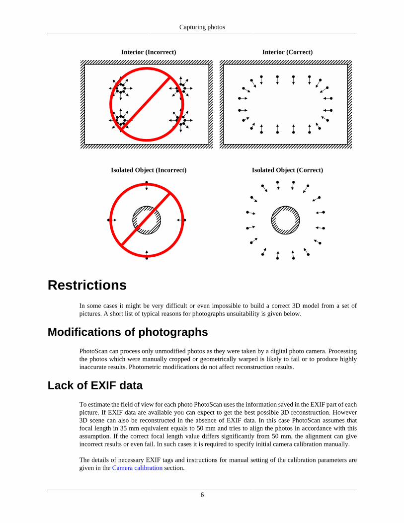
The following figures represent advice on appropriate capturing scenarios:
Facade (Incorrect) Facade (Correct)
Capturing photos
6
Interior (Incorrect) Interior (Correct)
Isolated Object (Incorrect) Isolated Object (Correct)
RestrictionsIn some cases it might be very difficult or even impossible to build a correct 3D model from a set ofpictures. A short list of typical reasons for photographs unsuitability is given below.
Modifications of photographs
PhotoScan can process only unmodified photos as they were taken by a digital photo camera. Processingthe photos which were manually cropped or geometrically warped is likely to fail or to produce highlyinaccurate results. Photometric modifications do not affect reconstruction results.
Lack of EXIF data
To estimate the field of view for each photo PhotoScan uses the information saved in the EXIF part of eachpicture. If EXIF data are available you can expect to get the best possible 3D reconstruction. However3D scene can also be reconstructed in the absence of EXIF data. In this case PhotoScan assumes thatfocal length in 35 mm equivalent equals to 50 mm and tries to align the photos in accordance with thisassumption. If the correct focal length value differs significantly from 50 mm, the alignment can giveincorrect results or even fail. In such cases it is required to specify initial camera calibration manually.
The details of necessary EXIF tags and instructions for manual setting of the calibration parameters aregiven in the Camera calibration section.
Capturing photos
7
Lens distortionThe distortion of the lenses used to capture the photos should be well simulated with the Brown's distortionmodel. Otherwise it is most unlikely that processing results will be accurate. Fisheye and ultra-wide anglelenses are poorly modeled by the common distortion model implemented in PhotoScan software, so it isrequired to choose proper camera type in Camera Calibration dialog prior to processing.
8
Chapter 3. General workflowProcessing of images with PhotoScan includes the following main steps:
• loading photos into PhotoScan;
• inspecting loaded images, removing unnecessary images;
• aligning photos;
• building dense point cloud;
• building mesh (3D polygonal model);
• generating texture;
• building tiled model;
• building digital elevation model;
• building orthomosaic;
• exporting results.
If you are using PhotoScan in the full function (not the Demo) mode, intermediate results of the imageprocessing can be saved at any stage in the form of project files and can be used later. The concept ofprojects and project files is briefly explained in the Saving intermediate results section.
The list above represents all the necessary steps involved in the construction of a textured 3D model ,DEM and orthomosaic from your photos. Some additional tools, which you may find to be useful, aredescribed in the successive chapters.
Preferences settingsBefore starting a project with PhotoScan it is recommended to adjust the program settings for your needs.In Preferences dialog (General Tab) available through the Tools menu you can indicate the path to thePhotoScan log file to be shared with the Agisoft support team in case you face any problem during theprocessing. Here you can also change GUI language to the one that is most convenient for you. The optionsare: English, Chinese, French, German, Japanese, Portuguese, Russian, Spanish.
On the OpenCL Tab you need to make sure that all OpenCL devices detected by the program are checked.PhotoScan exploits GPU processing power that speeds up the process significantly. If you have decidedto switch on GPUs for photogrammetric data processing with PhotoScan, it is recommended to free onephysical CPU core per each active GPU for overall control and resource managing tasks.
Loading photosBefore starting any operation it is necessary to point out what photos will be used as a source for 3Dreconstruction. In fact, photographs themselves are not loaded into PhotoScan until they are needed. So,when you "load photos" you only indicate photographs that will be used for further processing.
To load a set of photos
1.Select Add Photos... command from the Workflow menu or click Add Photos toolbar button onthe Workspace pane.
General workflow
9
2. In the Add Photos dialog box browse to the folder containing the images and select files to beprocessed. Then click Open button.
3. Selected photos will appear on the Workspace pane.
Note
• PhotoScan accepts the following image formats: JPEG, TIFF, PNG, BMP, PPM, OpenEXRand JPEG Multi-Picture Format (MPO). Photos in any other format will not be shown in theAdd Photos dialog box. To work with such photos you will need to convert them in one of thesupported formats.
If you have loaded some unwanted photos, you can easily remove them at any moment.
To remove unwanted photos
1. On the Workspace pane select the photos to be removed.
2. Right-click on the selected photos and choose Remove Items command from the opened context
menu, or click Remove Items toolbar button on the Workspace pane. The selected photos willbe removed from the working set.
Camera groupsIf all the photos or a subset of photos were captured from one camera position - camera station, forPhotoScan to process them correctly it is obligatory to move those photos to a camera group and markthe group as Camera Station. It is important that for all the photos in a Camera Station group distancesbetween camera centers were negligibly small compared to the camera-object minimal distance. 3D modelreconstruction will require at least two camera stations with overlapping photos to be present in a chunk.However, it is possible to export panoramic picture for the data captured from only one camera station.Refer to Exporting results section for guidance on panorama export.
Alternatively, camera group structure can be used to manipulate the image data in a chunk easily, e.g. toapply Disable/Enable functions to all the cameras in a group at once.
To move photos to a camera group
1. On the Workspace pane (or Photos pane) select the photos to be moved.
2. Right-click on the selected photos and choose Move Cameras - New Camera Group command fromthe opened context menu.
3. A new group will be added to the active chunk structure and selected photos will be moved to thatgroup.
4. Alternatively selected photos can be moved to a camera group created earlier using Move Cameras- Camera Group - Group_name command from the context menu.
To mark group as camera station, right click on the camera group name and select Set Group Typecommand from the context menu.
Inspecting loaded photosLoaded photos are displayed on the Workspace pane along with flags reflecting their status.
The following flags can appear next to the photo name:
General workflow
10
NC (Not calibrated)Notifies that the EXIF data available is not sufficient to estimate the camera focal length. In this casePhotoScan assumes that the corresponding photo was taken using 50mm lens (35mm film equivalent).If the actual focal length differs significantly from this value, manual calibration may be required.More details on manual camera calibration can be found in the Camera calibration section.
NA (Not aligned)Notifies that external camera orientation parameters have not been estimated for the current photo yet.
Images loaded to PhotoScan will not be aligned until you perform the next step - photos alignment.
Notifies that Camera Station type was assigned to the group.
Multispectral imageryPhotoScan supports processing of multispectral images saved as multichannel (single page) TIFF files.The main processing stages for multispectral images are performed based on the master channel, whichcan be selected by the user. During orthophoto export, all spectral bands are processed together to form amultispectral orthophoto with the same bands as in source images.
The overall procedure for multispectral imagery processing does not differ from the usual procedure fornormal photos, except the additional master channel selection step performed after adding images to theproject. For the best results it is recommended to select the spectral band which is sharp and as muchdetailed as possible.
To select master channel
1. Add multispectral images to the project using Add Photos... command from the Workflow menu or
Add Photos toolbar button.
2. Select Set Master Channel... command from the chunk context menu in the Workspace pane.
3. In the Set Master Channel dialog select the channel to be used as master and click OK button. Displayof images in PhotoScan window will be updated according to the master channel selection.
Note
• Set Master Channel... command is available for RGB images as well. You can either indicateonly one channel to be used as the basis for photogrammetric processing or leave the parametervalue as Default for all three channels to be used in processing.
Multispectral orthomosaic export is supported in GeoTIFF format only. When exporting in other formats,only master channel will be saved.
Rigid camera rigsPhotoScan supports processing of multispectral datasets captured with multiple synchronized camerasoperating in different spectral ranges. In this case multiple images (planes) are available for each positionand PhotoScan will estimate separate calibration for each plane as well as their relative orientation withincamera rig.
Multiplane layout is formed at the moment of adding photos to the chunk. It will reflect the data layoutused to store image files. Therefore it is necessary to organize files on the disk appropriately in advance.The following data layouts can be used with PhotoScan:
General workflow
11
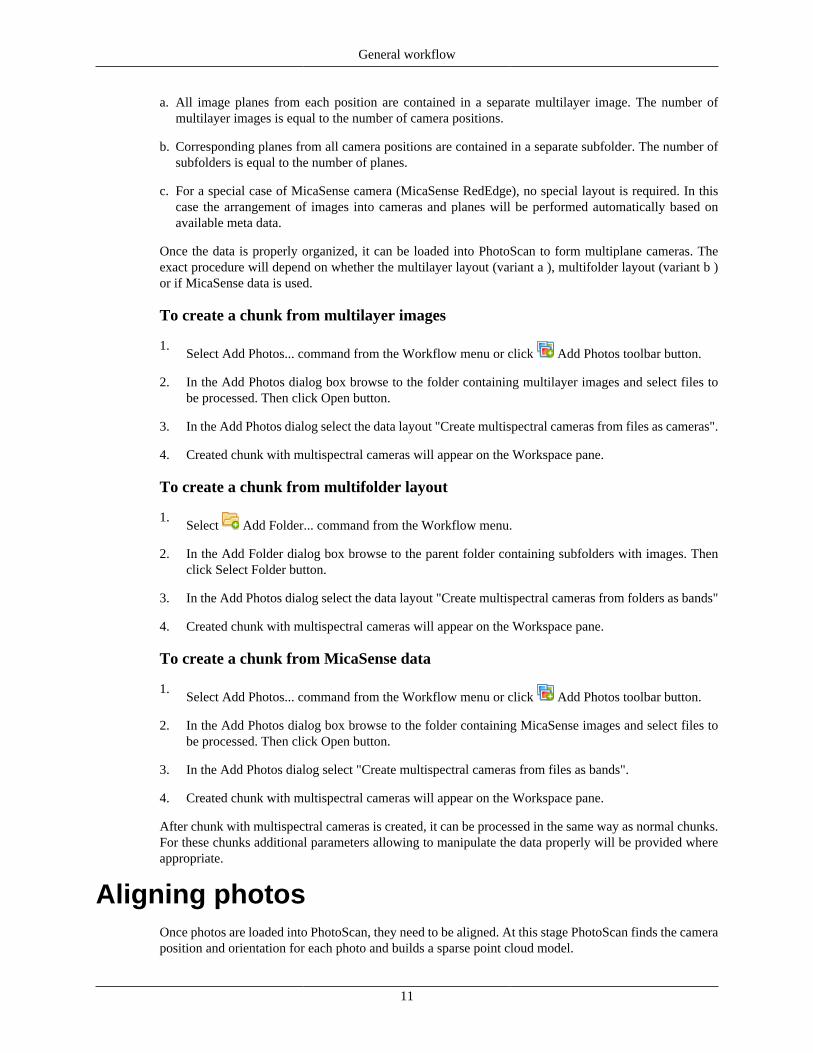
a. All image planes from each position are contained in a separate multilayer image. The number ofmultilayer images is equal to the number of camera positions.
b. Corresponding planes from all camera positions are contained in a separate subfolder. The number ofsubfolders is equal to the number of planes.
c. For a special case of MicaSense camera (MicaSense RedEdge), no special layout is required. In thiscase the arrangement of images into cameras and planes will be performed automatically based onavailable meta data.
Once the data is properly organized, it can be loaded into PhotoScan to form multiplane cameras. Theexact procedure will depend on whether the multilayer layout (variant a ), multifolder layout (variant b )or if MicaSense data is used.
To create a chunk from multilayer images
1.Select Add Photos... command from the Workflow menu or click Add Photos toolbar button.
2. In the Add Photos dialog box browse to the folder containing multilayer images and select files tobe processed. Then click Open button.
3. In the Add Photos dialog select the data layout "Create multispectral cameras from files as cameras".
4. Created chunk with multispectral cameras will appear on the Workspace pane.
To create a chunk from multifolder layout
1.Select Add Folder... command from the Workflow menu.
2. In the Add Folder dialog box browse to the parent folder containing subfolders with images. Thenclick Select Folder button.
3. In the Add Photos dialog select the data layout "Create multispectral cameras from folders as bands"
4. Created chunk with multispectral cameras will appear on the Workspace pane.
To create a chunk from MicaSense data
1.Select Add Photos... command from the Workflow menu or click Add Photos toolbar button.
2. In the Add Photos dialog box browse to the folder containing MicaSense images and select files tobe processed. Then click Open button.
3. In the Add Photos dialog select "Create multispectral cameras from files as bands".
4. Created chunk with multispectral cameras will appear on the Workspace pane.
After chunk with multispectral cameras is created, it can be processed in the same way as normal chunks.For these chunks additional parameters allowing to manipulate the data properly will be provided whereappropriate.
Aligning photosOnce photos are loaded into PhotoScan, they need to be aligned. At this stage PhotoScan finds the cameraposition and orientation for each photo and builds a sparse point cloud model.
General workflow
12
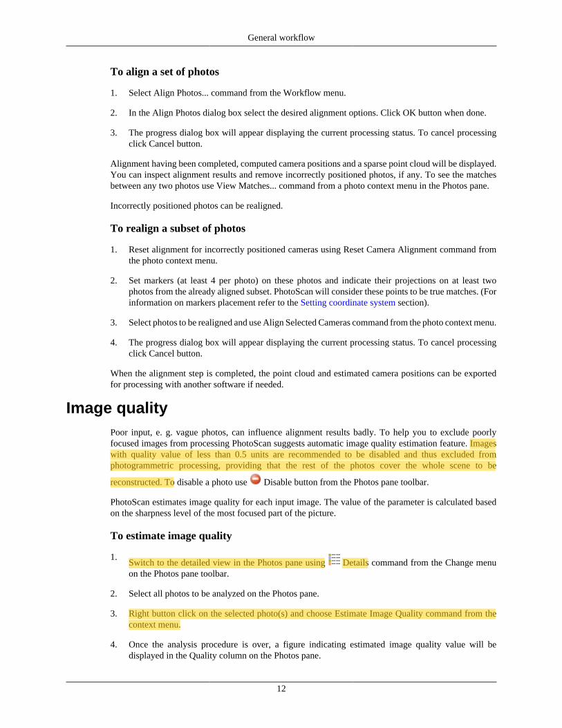
To align a set of photos
1. Select Align Photos... command from the Workflow menu.
2. In the Align Photos dialog box select the desired alignment options. Click OK button when done.
3. The progress dialog box will appear displaying the current processing status. To cancel processingclick Cancel button.
Alignment having been completed, computed camera positions and a sparse point cloud will be displayed.You can inspect alignment results and remove incorrectly positioned photos, if any. To see the matchesbetween any two photos use View Matches... command from a photo context menu in the Photos pane.
Incorrectly positioned photos can be realigned.
To realign a subset of photos
1. Reset alignment for incorrectly positioned cameras using Reset Camera Alignment command fromthe photo context menu.
2. Set markers (at least 4 per photo) on these photos and indicate their projections on at least twophotos from the already aligned subset. PhotoScan will consider these points to be true matches. (Forinformation on markers placement refer to the Setting coordinate system section).
3. Select photos to be realigned and use Align Selected Cameras command from the photo context menu.
4. The progress dialog box will appear displaying the current processing status. To cancel processingclick Cancel button.
When the alignment step is completed, the point cloud and estimated camera positions can be exportedfor processing with another software if needed.
Image qualityPoor input, e. g. vague photos, can influence alignment results badly. To help you to exclude poorlyfocused images from processing PhotoScan suggests automatic image quality estimation feature. Imageswith quality value of less than 0.5 units are recommended to be disabled and thus excluded fromphotogrammetric processing, providing that the rest of the photos cover the whole scene to be
reconstructed. To disable a photo use Disable button from the Photos pane toolbar.
PhotoScan estimates image quality for each input image. The value of the parameter is calculated basedon the sharpness level of the most focused part of the picture.
To estimate image quality
1.Switch to the detailed view in the Photos pane using Details command from the Change menuon the Photos pane toolbar.
2. Select all photos to be analyzed on the Photos pane.
3. Right button click on the selected photo(s) and choose Estimate Image Quality command from thecontext menu.
4. Once the analysis procedure is over, a figure indicating estimated image quality value will bedisplayed in the Quality column on the Photos pane.
wallin
Highlight
wallin
Highlight
wallin
Highlight
General workflow
13
Alignment parametersThe following parameters control the photo alignment procedure and can be modified in the Align Photosdialog box:
AccuracyHigher accuracy settings help to obtain more accurate camera position estimates. Lower accuracysettings can be used to get the rough camera positions in a shorter period of time.
While at High accuracy setting the software works with the photos of the original size, Medium settingcauses image downscaling by factor of 4 (2 times by each side), at Low accuracy source files aredownscaled by factor of 16, and Lowest value means further downscaling by 4 times more. Highestaccuracy setting upscales the image by factor of 4. Since tie point positions are estimated on thebasis of feature spots found on the source images, it may be meaningful to upscale a source phototo accurately localize a tie point. However, Highest accuracy setting is recommended only for verysharp image data and mostly for research purposes due to the corresponding processing being quitetime consuming.
Pair preselectionThe alignment process of large photo sets can take a long time. A significant portion of this time periodis spent on matching of detected features across the photos. Image pair preselection option may speedup this process due to selection of a subset of image pairs to be matched. In the Generic preselectionmode the overlapping pairs of photos are selected by matching photos using lower accuracy settingfirst.
In the Reference preselection mode the overlapping pairs of photos are selected based on themeasured camera locations (if present). For oblique imagery it is necessary to set Ground altitudevalue (average ground height in the same coordinate system which is set for camera coordinates data)in the Settings dialog of the Reference pane to make the preselection procedure work efficiently.Ground altitude information must be accompanied with yaw, pitch, roll data for cameras. Yaw, pitch,roll data should be input in the Reference pane.
Additionally the following advanced parameters can be adjusted.
Key point limitThe number indicates upper limit of feature points on every image to be taken into account duringcurrent processing stage. Using zero value allows PhotoScan to find as many key points as possible,but it may result in a big number of less reliable points.
Tie point limitThe number indicates upper limit of matching points for every image. Using zero value doesn't applyany tie point filtering.
Constrain features by maskWhen this option is enabled, masked areas are excluded from feature detection procedure. Foradditional information on the usage of masks please refer to the Using masks section.
Note
• Tie point limit parameter allows to optimize performance for the task and does not generallyeffect the quality of the further model. Recommended value is 4000. Too high or too low tie pointlimit value may cause some parts of the dense point cloud model to be missed. The reason is thatPhotoScan generates depth maps only for pairs of photos for which number of matching points isabove certain limit. This limit equals to 100 matching points, unless moved up by the figure "10%
General workflow
14
of the maximum number of matching points between the photo in question and other photos,only matching points corresponding to the area within the bounding box being considered."
• The number of tie points can be reduced after the alignment process with Tie Points - Thin PointCloud command available from Tools menu. As a results sparse point cloud will be thinned, yetthe alignment will be kept unchanged.
Point cloud generation based on imported camera dataPhotoScan supports import of external and internal camera orientation parameters. Thus, if precise cameradata is available for the project, it is possible to load them into PhotoScan along with the photos, to beused as initial information for 3D reconstruction job.
To import external and internal camera parameters
1. Select Import Cameras command from the Tools menu.
2. Select the format of the file to be imported.
3. Browse to the file and click Open button.
4. The data will be loaded into the software. Camera calibration data can be inspected in the CameraCalibration dialog, Adjusted tab, available from Tools menu. If the input file contains some referencedata (camera position data in some coordinate system), the data will be shown on the Reference pane,View Estimated tab.
Camera data can be loaded in one of the following formats: PhotoScan *.xml, BINGO *.dat, Bundler *.out,VisionMap Detailed Report *.txt, Realviz RZML *.rzml.
Once the data is loaded, PhotoScan will offer to build point cloud. This step involves feature pointsdetection and matching procedures. As a result, a sparse point cloud - 3D representation of the tie-pointsdata, will be generated. Build Point Cloud command is available from Tools - Tie Points menu. Parameterscontrolling Build Point Cloud procedure are the same as the ones used at Align Photos step (see above).
Building dense point cloudPhotoScan allows to generate and visualize a dense point cloud model. Based on the estimated camerapositions the program calculates depth information for each camera to be combined into a single densepoint cloud. PhotoScan tends to produce extra dense point clouds, which are of almost the same density,if not denser, as LIDAR point clouds. A dense point cloud can be edited and classified within PhotoScanenvironment or exported to an external tool for further analysis.
To build a dense point cloud
1.Check the reconstruction volume bounding box. To adjust the bounding box use the Resize Region
and Rotate Region toolbar buttons. Rotate the bounding box and then drag corners of the box tothe desired positions.
2. Select the Build Dense Cloud... command from the Workflow menu.
3. In the Build Dense Cloud dialog box select the desired reconstruction parameters. Click OK buttonwhen done.

General workflow
15
4. The progress dialog box will appear displaying the current processing status. To cancel processingclick Cancel button.
Reconstruction parametersQuality
Specifies the desired reconstruction quality. Higher quality settings can be used to obtain more detailedand accurate geometry, but they require longer time for processing. Interpretation of the qualityparameters here is similar to that of accuracy settings given in Photo Alignment section. The onlydifference is that in this case Ultra High quality setting means processing of original photos, whileeach following step implies preliminary image size downscaling by factor of 4 (2 times by each side).
Additionally the following advanced parameters can be adjusted.
Depth Filtering modesAt the stage of dense point cloud generation reconstruction PhotoScan calculates depth maps for everyimage. Due to some factors, like noisy or badly focused images, there can be some outliers amongthe points. To sort out the outliers PhotoScan has several built-in filtering algorithms that answer thechallenges of different projects.
If there are important small details which are spatially distingueshed in the scene to bereconstructed, then it is recommended to set Mild depth filtering mode, for important featuresnot to be sorted out as outliers. This value of the parameter may also be useful for aerial projectsin case the area contains poorly textued roofs, for example.
If the area to be reconstructed does not contain meaningful small details, then it is reasonableto chose Aggressive depth filtering mode to sort out most of the outliers. This value of theparameter normally recommended for aerial data processing, however, mild filtering may beuseful in some projects as well (see poorly textured roofs comment in the mild parameter valurdescription above).
Moderate depth filtering mode brings results that are in between the Mild and Aggressiveapproaches. You can experiment with the setting in case you have doubts which mode to choose.
Additionally depth filtering can be Disabled. But this option is not recommended as the resultingdense cloud could be extremely noisy.
Building meshTo build a mesh
1. Check the reconstruction volume bounding box. If the model has already been referenced, thebounding box will be properly positioned automatically. Otherwise, it is important to control itsposition manually.
To adjust the bounding box manually, use the Resize Region and Rotate Region toolbarbuttons. Rotate the bounding box and then drag corners of the box to the desired positions - only partof the scene inside the bounding box will be reconstructed. If the Height field reconstructionmethod is to be applied, it is important to control the position of the red side of the bounding box: itdefines reconstruction plane. In this case make sure that the bounding box is correctly oriented.
2. Select the Build Mesh... command from the Workflow menu.
3. In the Build Mesh dialog box select the desired reconstruction parameters. Click OK button whendone.

General workflow
16
4. The progress dialog box will appear displaying the current processing status. To cancel processingclick Cancel button.
Reconstruction parametersPhotoScan supports several reconstruction methods and settings, which help to produce optimalreconstructions for a given data set.
Surface type
Arbitrary surface type can be used for modeling of any kind of object. It should be selectedfor closed objects, such as statues, buildings, etc. It doesn't make any assumptions on the type ofthe object being modeled, which comes at a cost of higher memory consumption.
Height field surface type is optimized for modeling of planar surfaces, such as terrains orbasereliefs. It should be selected for aerial photography processing as it requires lower amountof memory and allows for larger data sets processing.
Source dataSpecifies the source for the mesh generation procedure. Sparse cloud can be used for fast 3Dmodel generation based solely on the sparse point cloud. Dense cloud setting will result in longerprocessing time but will generate high quality output based on the previously reconstructed densepoint cloud.
Polygon countSpecifies the maximum number of polygons in the final mesh. Suggested values (High, Medium,Low) are calculated based on the number of points in the previously generated dense point cloud: theration is 1/5, 1/15, and 1/45 respectively. They present optimal number of polygons for a mesh of acorresponding level of detail. It is still possible for a user to indicate the target number of polygonsin the final mesh according to their choice. It could be done through the Custom value of the Polygoncount parameter. Please note that while too small number of polygons is likely to result in too roughmesh, too huge custom number (over 10 million polygons) is likely to cause model visualizationproblems in external software.
Additionally the following advanced parameters can be adjusted.
Interpolation
If interpolation mode is Disabled it leads to accurate reconstruction results since only areascorresponding to dense point cloud points are reconstructed. Manual hole filling is usuallyrequired at the post processing step.
With Enabled (default) interpolation mode PhotoScan will interpolate some surface areaswithin a circle of a certain radius around every dense cloud point. As a result some holes can beautomatically covered. Yet some holes can still be present on the model and are to be filled atthe post processing step.
In Extrapolated mode the program generates holeless model with extrapolated geometry.Large areas of extra geometry might be generated with this method, but they could be easilyremoved later using selection and cropping tools.
Point classesSpecifies the classes of the dense point cloud to be used for mesh generation. For example, select only"Ground Points" to produce a DTM as opposed to a DSM. Preliminary Classifying dense cloud pointsprocedure should be performed for this option of mesh generation to be active.
General workflow
17
Note
• PhotoScan tends to produce 3D models with excessive geometry resolution, so it is recommendedto perform mesh decimation after geometry computation. More information on mesh decimationand other 3D model geometry editing tools is given in the Editing model geometry section.
Building model textureTo generate 3D model texture
1. Select Build Texture... command from the Workflow menu.
2. Select the desired texture generation parameters in the Build Texture dialog box. Click OK buttonwhen done.
3. The progress dialog box will appear displaying the current processing status. To cancel processingclick Cancel button.
Texture mapping modesThe texture mapping mode determines how the object texture will be packed in the texture atlas. Propertexture mapping mode selection helps to obtain optimal texture packing and, consequently, better visualquality of the final model.
GenericThe default mode is the Generic mapping mode; it allows to parametrize texture atlas for arbitrarygeometry. No assumptions regarding the type of the scene to be processed are made; program triesto create as uniform texture as possible.
Adaptive orthophotoIn the Adaptive orthophoto mapping mode the object surface is split into the flat part andvertical regions. The flat part of the surface is textured using the orthographic projection, while verticalregions are textured separately to maintain accurate texture representation in such regions. When inthe Adaptive orthophoto mapping mode, program tends to produce more compact texturerepresentation for nearly planar scenes, while maintaining good texture quality for vertical surfaces,such as walls of the buildings.
OrthophotoIn the Orthophoto mapping mode the whole object surface is textured in the orthographicprojection. The Orthophoto mapping mode produces even more compact texture representationthan the Adaptive orthophoto mode at the expense of texture quality in vertical regions.
SphericalSpherical mapping mode is appropriate only to a certain class of objects that have a ball-like form.It allows for continuous texture atlas being exported for this type of objects, so that it is much easierto edit it later. When generating texture in Spherical mapping mode it is crucial to set the Boundingbox properly. The whole model should be within the Bounding box. The red side of the Boundingbox should be under the model; it defines the axis of the spherical projection. The marks on the frontside determine the 0 meridian.
Single photoThe Single photo mapping mode allows to generate texture from a single photo. The photo to beused for texturing can be selected from 'Texture from' list.
General workflow
18
Keep uvThe Keep uv mapping mode generates texture atlas using current texture parametrization. It canbe used to rebuild texture atlas using different resolution or to generate the atlas for the modelparametrized in the external software.
Texture generation parameters
The following parameters control various aspects of texture atlas generation:
Texture from (Single photo mapping mode only)Specifies the photo to be used for texturing. Available only in the Single photo mapping mode.
Blending mode (not used in Single photo mode)Selects the way how pixel values from different photos will be combined in the final texture.
Mosaic - implies two-step approach: it does blending of low frequency component for overlappingimages to avoid seamline problem (weighted average, weight being dependent on a number ofparameters including proximity of the pixel in question to the center of the image), while highfrequency component, that is in charge of picture details, is taken from a single image - the one thatpresents good resolution for the area of interest while the camera view is almost along the normal tothe reconstructed surface in that point.
Average - uses the weighted average value of all pixels from individual photos, the weight beingdependent on the same parameters that are considered for high frequence component in mosaic mode.
Max Intensity - the photo which has maximum intensity of the corresponding pixel is selected.
Min Intensity - the photo which has minimum intensity of the corresponding pixel is selected.
Disabled - the photo to take the color value for the pixel from is chosen like the one for the highfrequency component in mosaic mode.
Texture size / countSpecifies the size (width & height) of the texture atlas in pixels and determines the number of filesfor texture to be exported to. Exporting texture to several files allows to archive greater resolution ofthe final model texture, while export of high resolution texture to a single file can fail due to RAMlimitations.
Additionally the following advanced parameters can be adjusted.
Enable color correctionThe feature is useful for processing of data sets with extreme brightness variation. However, pleasenote that color correction process takes up quite a long time, so it is recommended to enable the settingonly for the data sets that proved to present results of poor quality.
Note
• HDR texture generation requires HDR photos on input.
Improving texture quality
To improve resulting texture quality it may be reasonable to exclude poorly focused images fromprocessing at this step. PhotoScan suggests automatic image quality estimation feature. Images with quality
General workflow
19
value of less than 0.5 units are recommended to be disabled and thus excluded from texture generation
procedure. To disable a photo use Disable button from the Photos pane toolbar.
PhotoScan estimates image quality as a relative sharpness of the photo with respect to other images inthe data set. The value of the parameter is calculated based on the sharpness level of the most focusedpart of the picture.
To estimate image quality
1.Switch to the detailed view in the Photos pane using Details command from the Change menuon the Photos pane toolbar.
2. Select all photos to be analyzed on the Photos pane.
3. Right button click on the selected photo(s) and choose Estimate Image Quality command from thecontext menu.
4. Once the analysis procedure is over, a figure indicating estimated image quality value will bedisplayed in the Quality column on the Photos pane.
Building tiled modelHierarchical tiles format is a good solution for city scale modeling. It allows for responsive visualisation oflarge area 3D models in high resolution, a tiled model being opened with Agisoft Viewer - a complementarytool included in PhotoScan installer package.
Tiled model is build based on dense point cloud data. Hierarchical tiles are textured from the sourceimagery.
Note
• Build Tiled Model procedure can be performed only for projects saved in .PSX format.
To build a tiled model
1. Check the reconstruction volume bounding box - tiled model will be generated for the area within
bounding box only. To adjust the bounding box use the Resize Region and Rotate Regiontoolbar buttons. Rotate the bounding box and then drag corners of the box to the desired positions.
2. Select the Build Tiled Model... command from the Workflow menu.
3. In the Build Tiled model dialog box select the desired reconstruction parameters. Click OK buttonwhen done.
4. The progress dialog box will appear displaying the current processing status. To cancel processingclick Cancel button.
Reconstruction parametersPixel size (m)
Suggested value shows automatically estimated pixel size due to input imagery effective resolution.It can be set by the user in meters.
General workflow
20
Tile sizeTile size can be set in pixels. For smaller tiles faster visualisation should be expected.
Building digital elevation modelPhotoScan allows to generate and visualize a digital elevation model (DEM). A DEM represents a surfacemodel as a regular grid of height values. DEM can be rasterized from a dense point cloud, a sparse pointcloud or a mesh. Most accurate results are calculated based on dense point cloud data. PhotoScan enablesto perform DEM-based point, distance, area, volume measurements as well as generate cross-sections fora part of the scene selected by the user. Additionally, contour lines can be calculated for the model anddepicted either over DEM or Orthomosaic in Ortho view within PhotoScan environment. More informationon measurement functionality can be found in Performing measurements on DEM section.
Note
• Build DEM procedure can be performed only for projects saved in .PSX format.
• DEM can be calculated for referenced models only. So make sure that you have set a coordinatesystem for your model before going to build DEM operation. For guidance on Setting coordinatesystem please go to Setting coordinate system
DEM is calculated for the part of the model within the bounding box. To adjust the bounding box use the
Resize Region and Rotate Region toolbar buttons. Rotate the bounding box and then drag cornersof the box to the desired positions.
To build DEM
1. Select the Build DEM... command from the Workflow menu.
2. In the Build DEM dialog box set Coordinate system for the DEM.
3. Select source data for DEM rasterization.
4. Click OK button when done.
5. The progress dialog box will appear displaying the current processing status. To cancel processingclick Cancel button.
ParametersSource data
It is recommended to calculate DEM based on dense point cloud data. Preliminary elevation dataresults can be generated from a sparse point cloud, avoiding Build Dense Cloud step for time limitationreasons.
InterpolationIf interpolation mode is Disabled it leads to accurate reconstruction results since only areascorresponding to dense point cloud points are reconstructed.
With Enabled (default) interpolation mode PhotoScan will calculate DEM for all areas of thescene that are visible on at least one image. Enabled (default) setting is recommended forDEM generation.
General workflow
21
In Extrapolated mode the program generates holeless model with some elevation data beingextrapolated.
Point classesThe parameter allows to select a point class (classes) that will be used for DEM calculation.
To generate digital terrain model (DTM), it is necessary to classify dense cloud points first in order todivide them in at least two classes: ground points and the rest. Please refer to Classifying dense cloudpoints section to read about dense point cloud classification options. Select Ground value for Point classparameter in Build DEM dialog to generate DTM.
To calculate DEM for a particular part of the project, use Region section of the Build DEM dialog. Indicatecoordinates of the bottom left and top right corners of the region to be exported in the left and right columnsof the textboxes respectively. Suggested values indicate coordinates of the bottom left and top right cornersof the whole area to be rasterized, the area being defined with the bounding box.
Resolution value shows effective ground resolution for the DEM estimated for the source data. Size of theresulting DEM, calculated with respect to the ground resolution, is presented in Total size textbox.
Building orthomosaicOrthomosaic export is normally used for generation of high resolution imagery based on the source photosand reconstructed model. The most common application is aerial photographic survey data processing,but it may be also useful when a detailed view of the object is required. PhotoScan enables to performorthomosaic seamline editing for better visual results (see Orthomosaic seamlines editing section of themanual).
For multispectral imagery processing workflow Ortho view tab presents Raster Calculator tool for NDVIand other vegetation indices calculation to analyze crop problems and generate prescriptions for variablerate farming equipment. More information on NDVI calculation functionality can be found in Performingmeasurements on mesh section.
Note
• Build Orthomosaic procedure can be performed only for projects saved in .PSX format.
To build Orthomosaic
1. Select the Build Orthomosaic... command from the Workflow menu.
2. In the Build Orthomosaic dialog box set Coordinate system for the Orthomosaic referencing.
3. Select type of surface data for orthorectified imagery to be projected onto.
4. Click OK button when done.
5. The progress dialog box will appear displaying the current processing status. To cancel processingclick Cancel button.
PhotoScan allows to project the orthomosaic onto a plane set by the user, providing that mesh is selectedas a surface type. To generate orthomosaic in a planar projection choose Planar Projection Type inBuild Orthomosaic dialog. You can select projection plane and orientation of the orthomosaic. PhotoScanprovides an option to project the model to a plane determined by a set of markers (if there are no 3 markersin a desired projection plane it can be specified with 2 vectors, i. e. 4 markers). Planar projection typemay be useful for orthomosaic generation in projects concerning facades or surfaces that are not described
General workflow
22
with Z(X,Y) function. To generate an orthomosaic in planar projection, preliminary generation of meshdata is required.
ParametersSurface
Orthomosaic creation based on DEM data is especially efficient for aerial survey data processingscenarios allowing for time saving on mesh generation step. Alternatively, mesh surface type allowsto create orthomosaic for less common, yet quite demanded applications, like orthomosaic generationfor facades of the buildings or other models that might be not referenced at all.
Blending modeMosaic (default) - implements approach with data division into several frequency domainswhich are blended independently. The highest frequency component is blended along the seamlineonly, each further step away from the seamline resulting in a less number of domains being subjectto blending.Average - uses the weighted average value of all pixels from individual photos.Disabled - the color value for the pixel is taken from the photo with the camera view being almostalong the normal to the reconstructed surface in that point.
Enable color correctionColor correction feature is useful for processing of data sets with extreme brightness variation.However, please note that color correction process takes up quite a long time, so it is recommendedto enable the setting only for the data sets that proved to present results of poor quality before.
Pixel sizeDefault value for pixel size in Export Orthomosaic dialog refers to ground sampling resolution, thus,it is useless to set a smaller value: the number of pixels would increase, but the effective resolutionwould not. However, if it is meaningful for the purpose, pixel size value can be changed by the user.
Max. dimension (pix)The parameter allows to set maximal dimension for the resulting raster data.
PhotoScan generates orthomosaic for the whole area, where surface data is available. Bounding boxlimitations are not applied. To build orthomosaic for a particular (rectangular) part of the project use Regionsection of the Build Orthomosaic dialog. Indicate coordinates of the bottom left and top right corners of theregion to be exported in the left and right columns of the textboxes respectively. Estimate button allowsyou to see the coordinates of the bottom left and top right corners of the whole area.
Estimate button enables to control total size of the resulting orthomosaic data for the currently selectedreconstruction area (all available data (default) or a certain region (Region parameter)) and resolution(Pixel size or Max. dimension parameters). The information is shown in the Total size (pix) textbox.
Saving intermediate resultsCertain stages of 3D model reconstruction can take a long time. The full chain of operations couldeventually last for 4-6 hours when building a model from hundreds of photos. It is not always possible tocomplete all the operations in one run. PhotoScan allows to save intermediate results in a project file.
PhotoScan Archive files (*.psz) may contain the following information:
• List of loaded photographs with reference paths to the image files.
• Photo alignment data such as information on camera positions, sparse point cloud model and set ofrefined camera calibration parameters for each calibration group.
General workflow
23
• Masks applied to the photos in project.
• Depth maps for cameras.
• Dense point cloud model with information on points classification.
• Reconstructed 3D polygonal model with any changes made by user. This includes mesh and textureif it was built.
• List of added markers as well as of scale-bars and information on their positions.
• Structure of the project, i.e. number of chunks in the project and their content.
Note that since PhotoScan tends to generate extra dense point clouds and highly detailed polygonal models,project saving procedure can take up quite a long time. You can decrease compression level to speed up thesaving process. However, please note that it will result in a larger project file. Compression level settingcan be found on the Advanced tab of the Preferences dialog available from Tools menu.
The software also allows to save PhotoScan Project file (*.psx) which stores the links to the processingresults in *.psx file and the data itself in *.files structured archive. This format enables responsive loadingof large data (dense point clouds, meshes, etc.), thus avoiding delays on reopening a hundreds-of-photosproject. DEM and orthomosaic generation options are available only for projects saved in PSX format.
You can save the project at the end of any processing stage and return to it later. To restart work simplyload the corresponding file into PhotoScan. Project files can also serve as backup files or be used to savedifferent versions of the same model.
Project files use relative paths to reference original photos. Thus, when moving or copying the project fileto another location do not forget to move or copy photographs with all the folder structure involved aswell. Otherwise, PhotoScan will fail to run any operation requiring source images, although the projectfile including the reconstructed model will be loaded up correctly. Alternatively, you can enable Storeabsolute image paths option on the Advanced tab of the Preferences dialog available from Tools menu.
Exporting resultsPhotoScan supports export of processing results in various representations: sparse and dense point clouds,camera calibration and camera orientation data, mesh, etc. Orthomosaics and digital elevation models(both DSM and DTM), as well as tiled models can be generated according to the user requirements.
Point cloud and camera calibration data can be exported right after photo alignment is completed. All otherexport options are available after the corresponding processing step.
If you are going to export the results (point cloud / mesh / tiled model / orthomosaics) for the model that isnot referenced, please note that the resulting file will be oriented according to a default coordinate system(see axes in the bottom right corner of the Model view), i. e. the model can be shown differently from what
you see in PhotoScan window. To align the model orientation with the default coordinate system use Rotate object button from the Toolbar.
In some cases editing model geometry in the external software may be required. PhotoScan supports modelexport for editing in external software and then allows to import it back as it is described in the Editingmodel geometry section of the manual.
Main export commands are available from the File menu and the rest from the Export submenu of theTools menu.
General workflow
24
Point cloud export
To export sparse or dense point cloud
1. Select Export Points... command from the File menu.
2. Browse the destination folder, choose the file type, and print in the file name. Click Save button.
3. In the Export Points dialog box select desired Type of point cloud - Sparse or Dense.
4. Specify the coordinate system and indicate export parameters applicable to the selected file type,including the dense cloud classes to be saved.
5. Click OK button to start export.
6. The progress dialog box will appear displaying the current processing status. To cancel processingclick Cancel button.
Split in blocks option in the Export Points dialog can be useful for exporting large projects. It is availablefor referenced models only. You can indicate the size of the section in xy plane (in meters) for the pointcloud to be divided into respective rectangular blocks. The total volume of the 3D scene is limited withthe Bounding Box. The whole volume will be split in equal blocks starting from the point with minimumx and y values. Note that empty blocks will not be saved.
In some cases it may be reasonable to edit point cloud before exporting it. To read about point cloud editingrefer to the Editing point cloud section of the manual.
PhotoScan supports point cloud export in the following formats:
• Wavefront OBJ
• Stanford PLY
• XYZ text file format
• ASPRS LAS
• LAZ
• ASTM E57
• U3D
• potree
• Agisoft OC3
• Topcon CL3
Note
• Saving color information of the point cloud is supported by the PLY, E57, LAS, LAZ, OC3,CL3 and TXT file formats.
• Saving point normals information is supported by the OBJ, PLY and TXT file formats.
General workflow
25
Tie points data export
To export matching points
1. Select Export Matches... command from the Tools menu.
2. Browse the destination folder, choose the file type, and print in the file name. Click Save button.
3. In the Export Matches dialog box set export parameters. Precision value sets the limit to the numberof decimal digits in the tie points coordinates to be saved.
4. Click OK button to start export.
5. The progress dialog box will appear displaying the current processing status. To cancel processingclick Cancel button.
PhotoScan supports matching points data export in the following formats:
• BINGO (*.dat) - saves original intrinsic and extrinsic camera data along with matching pointscoordinates.
• ORIMA (*.txt)
• PATB (*.ptb)
Matching points exported from PhotoScan can be used as a basis for AT procedure to be performed insome external software. Later on, estimated camera data can be imported back to PhotoScan (using ImportCameras command from the Tools menu) to proceed with 3D model reconstruction procedure.
Camera calibration and orientation data exportTo export camera calibration and camera orientation data select Export Cameras... command from theTools menu.
PhotoScan supports camera data export in the following formats:
• Agisoft XML structure
• Bundler OUT file format
• CHAN file format
• Boujou TXT file format
• Omega Phi Kappa text file format
• PATB Exterior orientation
• BINGO Exterior orientation
• AeroSys Exterior orientation
• Inpho project file
Note
• Camera data export in Bundler and Boujou file formats will save sparse point cloud data in thesame file.
General workflow
26
• Camera data export in Bundler file format would not save distortion coefficients k3, k4.
To export / import only camera calibration data select Camera Calibration... command from the Tools
menu. Using / buttons it is possible to load / save camera calibration data in the following formats:
• Agisoft Camera Calibration (*.xml)
• Australis Camera Parameters (*.txt)
• PhotoModeler Camera Calibration (*.ini)
• 3DM CalibCam Camera Parameters (*.txt)
• CalCam Camera Calibration (*.cal)
• Inpho Camera Calibration (*.txt)
Panorama exportPhotoScan is capable of panorama stitching for images taken from the same camera position - camerastation. To indicate for the software that loaded images have been taken from one camera station, oneshould move those photos to a camera group and assign Camera Station type to it. For information oncamera groups refer to Loading photos section.
To export panorama
1. Select Export - Export Panorama... command from the Tools menu.
2. Select camera group which panorama should be previewed for.
3. Choose panorama orientation in the file with the help of navigation buttons to the right of the previewwindow in the Export Panorama dialog.
4. Set exporting parameters: select camera groups which panorama should be exported for and indicateexport file name mask.
5. Click OK button
6. Browse the destination folder and click Save button.
Additionally, you can set boundaries for the region of panorama to be exported using Setup boundariessection of the Export Panorama dialog. Text boxes in the first line (X) allow to indicate the angle in thehorizontal plane and the second line (Y) serves for angle in the vertical plane limits. Image size optionenables to control the size of the exporting file.
3D model export
To export 3D model
1. Select Export Model... command from the File menu.
2. Browse the destination folder, choose the file type, and print in the file name. Click Save button.
3. In the Export Model dialog specify the coordinate system and indicate export parameters applicableto the selected file type.

General workflow
27
4. Click OK button to start export.
5. The progress dialog box will appear displaying the current processing status. To cancel processingclick Cancel button.
Note
• If the model is exported in local coordinates, PhotoScan can write a KML file for the exportedmodel to be correctly located on Google Earth.
If a model generated with PhotoScan is to be imported in a 3D editor program for inspection or furtherediting, it might be helpful to use Shift function while exporting the model. It allows to set the value tobe subtracted from the respective coordinate value for every vertex in the mesh. Essentially, this meanstranslation of the model coordinate system origin, which may be useful since some 3D editors, for example,truncate the coordinates values up to 8 or so digits, while in some projects they are decimals that makesense with respect to model positioning task. So it can be recommended to subtract a value equal to thewhole part of a certain coordinate value (see Reference pane, Camera coordinates values) before exportingthe model, thus providing for a reasonable scale for the model to be processed in a 3D editor program.
PhotoScan supports model export in the following formats:
• Wavefront OBJ
• 3DS file format
• VRML
• COLLADA
• Stanford PLY
• STL models
• Autodesk FBX
• Autodesk DXF
• Google Earth KMZ
• U3D
• Adobe PDF
Some file formats (OBJ, 3DS, VRML, COLLADA, PLY, FBX) save texture image in a separate file. Thetexture file should be kept in the same directory as the main file describing the geometry. If the textureatlas was not built only the model geometry is exported.
PhotoScan supports direct uploading of the models to Sketchfab resource. To publish your model onlineuse Upload Model... command from the File menu.
Tiled model export
To export tiled model
1. Select Export Tiled Model... command from the File menu.
General workflow
28
2. Browse the destination folder, choose the file type, and print in the file name. Click Save button.
3. The progress dialog box will appear displaying the current processing status. To cancel processingclick Cancel button.
PhotoScan supports tiled model export in the following formats:
• PhotoMesh Layer (*.zip)
• Agisoft Tiled Model (*.tls)
• Agisoft Tile Archive (*.zip)
Agisoft Tiled Model can be visualised in Agisoft Viewer application, which is included in AgisoftPhotoScan Professional installation file. Thanks to hierarchical tiles format, it allows to responsivelyvisualise large models.
Orthomosaic export
To export Orthomosaic
1. Select Export Orthomosaic... command from the File menu.
2. In the Export Orthomosaic dialog box specify coordinate system for the Orthomosaic to be saved in.
3. Check Write KML file and / or Write World file options to create files needed to georeference theorthomosaic in the Google Earth and / or a GIS .
4. Click Export button to start export.
5. Browse the destination folder, choose the file type, and print in the file name. Click Save button.
6. The progress dialog box will appear displaying the current processing status. To cancel processingclick Cancel button.
Note
• Write KML file option is available only if the model is georeferenced in WGS84 coordinatesystem due to the fact that Google Earth supports only this coordinate system.
• World file specifies coordinates of the four angle vertices of the exporting orthomosaic. Thisinformation is already included in GeoTIFF file, however, you could duplicate it for somereason. If you need to export orthomosaic in JPEG or PNG file formats and would like to havegeoreferencing data this informations could be useful.
If the export file of a fixed size is needed, it is possible to set the length of the longer side of the exportfile in Max. dimension (pix) parameter. The length should be indicated in pixels.
Split in blocks option in the Export Orthomosaic dialog can be useful for exporting large projects. Youcan indicate the size of the blocks (in pix) for the orthomosaic to be divided into. The whole area will besplit in equal blocks starting from the point with minimum x and y values. Note that empty blocks willnot be saved.
To export a particular part of the project use Region section of the Export Orthomosaic dialog. Indicatecoordinates of the bottom left and top right corners of the region to be exported in the left and right columns
General workflow
29
of the textboxes respectively. Estimate button allows you to see the coordinates of the bottom left and topright corners of the whole area.
Alternatively, you can indicate the region to be exported using polygon drawing option in the Ortho viewtab of the program window. (For instructions on polygon drawing refer to Shapes section of the manual.)Once the polygon is drawn, right-click on the polygon and set it as a boundary of the region to be exportedusing Set Boundary Type option from the context menu.
Default value for pixel size in Export Orthomosaic dialog refers to ground sampling resolution, thus, itis useless to set a smaller value: the number of pixels would increase, but the effective resolution wouldnot. If you have chosen to export orthomosaic with a certain pixel size (not using Max. dimension (pix)option), it is recommended to check estimated Total size (pix) of the resulting file to be sure that it is nottoo large to be correctly saved to the targeted file format.
For (Geo)TIFF export compression type may be set by the user. The following options are available:LZW, JPEG, Packbits, Deflate. Additionally, the file may be saved without compression (None valueof the compression type parameter). Write BigTIFF file option allows to save files bigger than standardTIFF limit of 4Gb. Total size textbox in the Export Orthomosaic dialog helps to estimate the size of theresulting file. However, it is recommended to make sure that the application you are planning to open theorthomosaic with supports BigTIFF format. Alternatively, you can split a large orthomosaic in blocks,with each block fitting the limits of a standard TIFF file.
While exporting orthomosaic in JPEG format, JPEG quality parameter controls balance betweencompression level (i.e. quality of the result) and export file size: the higher the value of the parameter (%)the more emphasis is on the quality at the expense of a larger resulting file.
The following formats are supported for orthomosaic export:
• JPEG
• PNG
• TIFF
• GeoTIFF
• Multiresolution Google Earth KML mosaic.
• Google Map Tiles.
• MBTiles.
• World Wind Tiles.
PhotoScan supports direct uploading of the orthomosaics to MapBox platform. To publish yourorthomosaic online use Upload Orthomosaic... command from the File menu.
Note
• MapBox upload requires secure token with uploads:write scope that should be obtained onthe account page of the MapBox web-site. Secure token shouldn't be mixed up with the publictoken, as the latter doesn't allow to upload orthomosaics from PhotoScan.
Multispectral orthomosaic export is supported in GeoTIFF format only. When exporting in other formats,only master channel will be saved. Multispectral orthomosaic has all channels of the original imagery plusalpha channel, transparency being used for no-data areas of the orthomosaic.

General workflow
30
To export Multispectral orthomosaic
1. Select Export Orthomosaic... command from the File menu.
2. Follow steps 2-4 from Orthomosaic export procedure above.
3. Browse the destination folder, choose GeoTIFF type, and print in the file name. Click Save button.
4. The progress dialog box will appear displaying the current processing status. To cancel processingclick Cancel button.
NDVI data export
Vegetation index data export is available with the Export Orthomosaic... command from the File menu.Vegetation index data can be saved as two types of data: as a grid of floating point index values calculatedper pixel of orthomosaic or as an orthomosaic in pseudocolors according to a pallet set by user. The formatis controlled with Raster transform option in Export Orthomosaic / Export Google KMZ / Export GoogleMap Tiles / Export MBTiles / Export World Wind Tiles dialogs. None value allows to export orthomosaicgenerated for the data before any index calculation procedure was performed.
DEM (DSM/DTM) exportPhotoScan allows to calculate and then export both a digital surface model (DSM) and a digital terrainmodel (DTM) (see Building digital elevation model section).
To export DEM
1. Select Export DEM... command from the File menu.
2. In the Export DEM dialog specify coordinate system to georeference the DEM.
3. Check Write KML file and/or Write World file options to create files needed to georeference theDEM in the Google Earth and/or a GIS.
4. Click Export button to start export.
5. Browse the destination folder, choose the file type, and print in the file name. Click Save button.
6. The progress dialog box will appear displaying the current processing status. To cancel processingclick Cancel button.
Note
• Write KML file option is available only if the model is georeferenced in WGS84 coordinatesystem due to the fact that Google Earth supports only this coordinate system.
• World file specifies coordinates of the four angle vertices of the exporting DEM. This informationis already included in GeoTIFF elevation data as well as in other supported file formats for DEMexport, however, you could duplicate it for some reason.
If export file of a fixed size is needed, it is possible to to set the length of the longer side of the export filein Max. dimension (pix) parameter. The length should be indicated in pixels.
Unlike orthophoto export, it is sensible to set smaller pixel size compared to the default value in DEMexport dialog; the effective resolution will increase. If you have chosen to export DEM with a certain pixel
General workflow
31
size (not using Max. dimension (pix) option), it is recommended to check estimated Total size (pix) of theresulting file to be sure that it is not too large to be correctly saved to the targeted file format.
No-data value is used for the points of the grid, where elevation value could not be calculated based onthe source data. Default value is suggested according to the industry standard, however it can be changedby user.
Split in blocks option in the Export DEM dialog can be useful for exporting large projects or meetingspecial DEM requirements. (See Orthomosaic export section for details.)
To export a particular part of the project use Region section of the Export DEM dialog. (See Orthomosaicexport section for details.) Similarly to orthomosaic export, polygons drawn over the DEM on the Orthotab of the program window can be set as boundaries for DEM export. (For instructions on polygon drawingrefer to Shapes section of the manual.)
The following formats are supported for DEM export:
• GeoTIFF elevation data
• Arc/Info ASCII Grid (ASC)
• Band interleaved file format (BIL)
• XYZ file format
• Sputnik KMZ
Extra products to exportIn addition to main targeted products PhotoScan allows to export several other processing results, like
• Undistort photos, i. e. photos free of lens distortions (Undistort Photos... command available from Exportsubmenu of the Tools menu).
• Depth map for any image (Export Depth... command available from photo context menu).
• Orthophotos for individual images (Export Orthophotos... command available from Export submenu ofthe Tools menu).
PhotoScan supports direct uploading of the models to Sketchfab resource and of the orthomosaicsto MapBox platform. To publish your model/orthomosaic online use Upload Model... and UploadOrthomosaic... command from the File menu.
Processing report generationPhotoScan supports automatic processing report generation in PDF format, which contains the basicparameters of the project, processing results and accuracy evaluations.
To generate processing report
1. Select Generate Report... command from the File menu.
2. Browse the destination folder, choose the file type, and print in the file name. Click Save button.
3. The progress dialog box will appear displaying the current processing status. To cancel processingclick Cancel button.
General workflow
32
PhotoScan processing report presents the following data:
• Orthomosaic sketch.
• Survey data including coverage area, flying altitude, GSR, general camera(s) info, as well as overlapstatistics.
• Camera calibration results: figures and an illustration for every sensor involved in the project.
• Camera positioning error estimates.
• Ground control points error estimates.
• Scale bars estimated distances and measurement errors.
• Digital elevation model sketch with resolution and point density info.
• Processing parameters used at every stage of the project.
Note
• Processing report can be exported after alignment step. Processing report export option isavailable for georeferenced projects only.
Survey Data
Number of images - total number of images uploaded into the project.
Camera stations - number of aligned images.
Flying altitude - average height above ground level.
Tie points - total number of valid tie points (equals to the number of points in the sparse cloud).
Ground resolution - effective ground resolution averaged over all aligned images.
Projections - total number of projections of valid tie points.
Coverage area - size of the area that has been surveyed.
Reprojection error - root mean square reprojection error averaged over all tie points on all images.
Reprojection error is the distance between the point on the image where a reconstructed 3D point can beprojected and the original projection of that 3D point detected on the photo and used as a basis for the3D point reconstruction procedure.
Camera Calibration
For precalibrated cameras internal parameters input by the user are shown on the report page. If a camerawas not precalibrated, internal camera parameters estimated by PhotoScan are presented.
Camera Locations
X error (m) - root mean square error for X coordinate for all the cameras.
Y error (m) - root mean square error for Y coordinate for all the cameras.
General workflow
33
XY error (m) - root mean square error for X and Y coordinates for all the cameras.
Z error (m) - root mean square error for Z coordinate for all the cameras.
Total error (m) - root mean square error for X, Y, Z coordinates for all the cameras.
Total error = sqrt(Sumi=1n [(Xi, est - Xi, in)2 + (Yi, est - Yi, in)2 + (Zi, est - Zi, in)2] / n)
Xi, in - input value for X coordinate for i camera position,
Xi, est - estimated value for X coordinate for i camera position,
Yi, in - input value for Y coordinate for i camera position,
Yi, est - estimated value for Y coordinate for i camera position,
Zi, in - input value for Z coordinate for i camera position,
Zi, est - estimated value for Z coordinate for i camera position,
Ground Control Points
XY error (m) - root mean square error for X and Y coordinates for a GCP location / check point.
Z error (m) - error for Z coordinate for a GCP location / check point.
Error (m) - root mean square error for X, Y, Z coordinates for a GCP location / check point.
Projections - number of projections for a GCP location / check point over all the images.
Error (pix) - root mean square error for X, Y coordinates on an image for a GCP location / checkpoint averaged over all the images.
Total - implies averaging over all the GCP locations / check points.
Scale Bars
Distance (m) - scale bar length estimated by PhotoScan.
Error (m) - difference between input and estimated values for scale bar length.
Total - implies averaging over all the scale bars in Control/Check section.
Digital Elevation Model
Resolution - effective resolution of the exported DEM. The value depends on the Quality parametervalue used at Build point cloud step, providing that DEM has been generated from dense point cloud.
Point Density - average number of dense cloud points per square meter.
Processing Parameters
Processing report contains processing parameters information, which is also available form Chunk contextmenu. Along with the values of the parameters used at various processing stages, this page of the reportpresents information on processing time. Processing time attributed to Dense point cloud processing stepwill exclude time spent on depth maps reconstruction, unless Keep depth maps option is checked on
General workflow
34
Advanced tab of Preferences dialog available from Tools menu. For projects calculated over networkprocessing time will not be shown.
PhotoScan matches images on different scales to improve robustness with blurred or difficult to matchimages. The accuracy of tie point projections depends on the scale at which they were located. PhotoScanuses information about scale to weight tie point reprojection errors. In the Reference pane settings dialogtie point accuracy parameter now corresponds to normalized accuracy - i.e. accuracy of tie point detectedat the scale equal to 1. Tie points detected on other scales will have accuracy proportional to their scales.This helps to obtain more accurate bundle adjustment results. On the processing parameters page of thereport (as well as in chunk information dialog) two reprojection errors are provided: the reprojection errorin the units of tie point scale (this is the quantity that is minimized during bundle adjustment), and thereprojection error in pixels (for convenience). The mean key point size value is a mean tie point scaleaveraged across all projections.
35
Chapter 4. ReferencingCamera calibration
Calibration groupsWhile carrying out photo alignment PhotoScan estimates both internal and external camera orientationparameters, including nonlinear radial distortions. For the estimation to be successful it is crucial to applythe estimation procedure separately to photos taken with different cameras. Once photos have been loadedin the program, PhotoScan automatically divides them into calibration groups according to the imageresolution and/or EXIF metadata like camera type and focal length. All the actions described below couldand should be applied (or not applied) to each calibration group individually.
Calibration groups can be rearranged manually.
To create a new calibration group
1. Select Camera Calibration... command from the Tools menu.
2. In the Camera Calibration dialog box, select photos to be arranged in a new group.
3. In the right-click context menu choose Create Group command.
4. A new group will be created and depicted on the left-hand part of the Camera Calibration dialog box.
To move photos from one group to another
1. Select Camera Calibration... command from the Tools menu.
2. In the Camera Calibration dialog box choose the source group on the left-hand part of the dialog.
3. Select photos to be moved and drag them to the target group on the left-hand part of the CameraCalibration dialog box.
To place each photo into a separate group you can use Split Groups command available at the right buttonclick on a calibration group name in the left-hand part of the Camera Calibration dialog
Camera typesPhotoScan supports four major types of camera: frame camera, fisheye camera, spherical camera andcylindrical camera. Camera type can be set in Camera Calibration dialog box available from Tools menu.
Frame camera. If the source data within a calibration group was shot with a frame camera, for successfulestimation of camera orientation parameters the information on approximate focal length (pix) is required.Obviously, to calculate focal length value in pixel it is enough to know focal length in mm along with thesensor pixel size in mm. Normally this data is extracted automatically from the EXIF metadata.
Frame camera with Fisheye lens. If extra wide lenses were used to get the source data, standardPhotoScan camera model will not allow to estimate camera parameters successfully. Fisheye camera typesetting will initialize implementation of a different camera model to fit ultra-wide lens distortions.
Spherical camera (equirectangular projection). In case the source data within a calibration groupwas shot with a spherical camera, camera type setting will be enough for the program to calculate
Referencing
36
camera orientation parameters. No additional information is required except the image in equirectangularrepresentation.
Spherical camera Cylindrical projection. In case the source data within a calibration group is a setof panoramic images stitched according to cylindrical model, camera type setting will be enough for theprogram to calculate camera orientation parameters. No additional information is required.
In case source images lack EXIF data or the EXIF data is insufficient to calculate focal length in pixels,PhotoScan will assume that focal length equals to 50 mm (35 mm film equivalent). However, if the initialguess values differ significantly from the actual focal length, it is likely to lead to failure of the alignmentprocess. So, if photos do not contain EXIF metadata, it is preferable to specify focal length (mm) and sensorpixel size (mm) manually. It can be done in Camera Calibration dialog box available from Tools menu.Generally, this data is indicated in camera specification or can be received from some online source. Toindicate to the program that camera orientation parameters should be estimated based on the focal lengthand pixel size information, it is necessary to set the Type parameter on the Initial tab to Auto value.
Camera calibration parametersOnce you have tried to run the estimation procedure and got poor results, you can improve them thanksto the additional data on calibration parameters.
To specify camera calibration parameters
1. Select Camera Calibration... command from the Tools menu.
2. Select calibration group, which needs reestimation of camera orientation parameters on the left sideof the Camera Calibration dialog box.
3. In the Camera Calibration dialog box, select Initial tab.
4. Modify the calibration parameters displayed in the corresponding edit boxes.
5. Set the Type to the Precalibrated value.
6. Repeat to every calibration group where applicable.
7. Click OK button to set the calibration.
Note
• Alternatively, initial calibration data can be imported from file using Load button on the Initialtab of the Camera Calibration dialog box. In addition to Agisoft calibration calibration file formatit is possible to import data from Australis, PhotoModeler, 3DM CalibCam, CalCam.
Initial calibration data will be adjusted during the Align Photos processing step. Once Align Photosprocessing step is finished adjusted calibration data will be displayed on the Adjusted tab of the CameraCalibration dialog box.
If very precise calibration data is available, to protect it from recalculation one should check Fix calibrationbox. In this case initial calibration data will not be changed during Align Photos process.
Adjusted camera calibration data can be saved to file using Save button on the Adjusted tab of the CameraCalibration dialog box.
Estimated camera distortions can be seen on the distortion plot available from context menu of a cameragroup in the Camera Calibration dialog. In addition, residuals graph (the second tab of the same DistortionPlot dialog) allows to evaluate how adequately the camera is described with the applied mathematical

Referencing
37
model. Note that residuals are averaged per cell of an image and then across all the images in a cameragroup. Scale reference under the plot indicates the scale of the distortions/residuals.
Calibration parameters listfx, fy
Focal length in x- and y-dimensions measured in pixels.
cx, cyPrincipal point coordinates, i.e. coordinates of lens optical axis interception with sensor plane.
skewSkew transformation coefficient.
k1, k2, k3, k4Radial distortion coefficients.
p1, p2, p3, p4Tangential distortion coefficients.
Setting coordinate systemMany applications require data with a defined coordinate system. Setting the coordinate system alsoprovides a correct scaling of the model allowing for surface area and volume measurements and makesmodel loading in geoviewers and geoinformation software much easier. Some functionality like digitalelevation model export is available only after the coordinate system is defined.
PhotoScan supports setting a coordinate system based on either ground control point (marker) coordinatesor camera coordinates. In both cases the coordinates are specified in the Reference pane and can be eitherloaded from the external file or typed in manually.
Setting coordinate system based on recorded camera positions is often used in aerial photographyprocessing. However it may be also useful for processing photos captured with GPS enabled cameras.Placing markers is not required if recorded camera coordinates are used to initialize the coordinate system.
In the case when ground control points are used to set up the coordinate system the markers should beplaced in the corresponding locations of the scene.
Using camera positioning data for georeferencing the model is faster since manual marker placement isnot required. On the other hand, ground control point coordinates are usually more accurate than telemetrydata, allowing for more precise georeferencing.
Placing markersPhotoScan uses markers to specify locations within the scene. Markers are used for setting up a coordinatesystem, photo alignment optimization, measuring distances and volumes within the scene as well as formarker based chunk alignment. Marker positions are defined by their projections on the source photos.The more photos are used to specify marker position the higher is accuracy of marker placement. To definemarker location within a scene it should be placed on at least 2 photos.
Note
• Marker placement is not required for setting the coordinate system based on recorded cameracoordinates. This section can be safely skipped if the coordinate system is to be defined basedon recorded camera locations.
Referencing
38
PhotoScan supports two approaches to marker placement: manual marker placement and guided markerplacement. Manual approach implies that the marker projections should be indicated manually on eachphoto where the marker is visible. Manual marker placement does not require 3D model and can beperformed even before photo alignment.
In the guided approach marker projection is specified for a single photo only. PhotoScan automaticallyprojects the corresponding ray onto the model surface and calculates marker projections on the rest ofthe photos where marker is visible. Marker projections defined automatically on individual photos can befurther refined manually. Reconstructed 3D model surface is required for the guided approach.
Guided marker placement usually speeds up the procedure of marker placement significantly and alsoreduces the chance of incorrect marker placement. It is recommended in most cases unless there are anyspecific reasons preventing this operation.
To place a marker using guided approach
1. Open a photo where the marker is visible by double clicking on its name.
2.Switch to the marker editing mode using Edit Markers toolbar button.
3. Right click on the photo at the point corresponding to the marker location.
4. Select Create Marker command from the context menu. New marker will be created and its projectionson the other photos will be automatically defined.
Note
• If the 3D model is not available or the ray at the selected point does not intersect with the modelsurface, the marker projection will be defined on the current photo only.
• Guided marker placement can be performed in the same way from the 3D view by right clicking
on the corresponding point on the model surface and using Create Marker command from thecontext menu. While the accuracy of marker placement in the 3D view is usually much lower, itmay be still useful for quickly locating the photos observing the specified location on the model.
To view the corresponding photos use Filter by Markers command again from the 3D viewcontext menu. If the command is inactive, please make sure that the marker in question is selectedon the Reference pane.
To place a marker using manual approach
1.Create marker instance using Add marker button on the Workspace pane or by Add Markercommand from the Chunk context menu (available by right clicking on the chunk title on theWorkspace pane).
2. Open the photo where the marker projection needs to be added by double clicking on the photos name.
3.Switch to the marker editing mode using Edit Markers toolbar button.
4. Right click at the point on the photo where the marker projection needs to be placed. From the contextmenu open Place Marker submenu and select the marker instance previously created. The markerprojection will be added to the current photo.
5. Repeat the previous step to place marker projections on other photos if needed.
Referencing
39
To save up time on manual marker placement procedure PhotoScan offers guiding lines feature. When amarker is placed on an aligned photo, PhotoScan highlights lines, which the marker is expected to lie on,on the rest of the aligned photos.
Note
• If a marker has been placed on at least two aligned images PhotoScan will find the marker
projections on the rest of the photos. The calculated marker positions will be indicated with icon on the corresponding aligned photos in Photo View mode.
Automatically defined marker locations can be later refined manually by dragging their projections on thecorresponding photos.
To refine marker location
1. Open the photo where the marker is visible by double clicking on the photo's name. Automatically
placed marker will be indicated with icon.
2.Switch to the marker editing mode using Edit Markers toolbar button.
3. Move the marker projection to the desired location by dragging it using left mouse button. Once the
marker location is refined by user, the marker icon will change to
Note
• To list photos where the marker locations are defined, select the corresponding marker on the
Workspace pane. The photos where the marker is placed will be marked with a icon on the
Photos pane. To filter photos by marker use Filter by Markers command from the 3D viewcontext menu.
In those cases when there are hesitations about the features depicted on the photo, comparative inspectionof two photos can prove to be useful. To open two photos in PhotoScan window simultaneously Move toOther Tab Group command is available from photo tab header context menu.
To open two photos simultaneously
1. In the Photos pane double click on one photo to be opened. The photo will be opened in a new tabof the main program window.
2. Right click on the tab header and choose Move to Other Tab Group command from the context menu.The main program window will be divided into two parts and the photo will be moved to the secondpart.
3. The next photo you will choose to be opened with a double click will be visualized in the active tabgroup.
PhotoScan automatically assigns default labels for each newly created marker. These labels can be changedusing the Rename... command from the marker context menu in the Workspace / Reference pane.
Assigning reference coordinatesTo reference the model the real world coordinates of at least 3 points of the scene should bespecified. Depending on the requirements, the model can be referenced using marker coordinates, camera
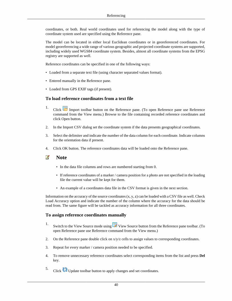
Referencing
40
coordinates, or both. Real world coordinates used for referencing the model along with the type ofcoordinate system used are specified using the Reference pane.
The model can be located in either local Euclidean coordinates or in georeferenced coordinates. Formodel georeferencing a wide range of various geographic and projected coordinate systems are supported,including widely used WGS84 coordinate system. Besides, almost all coordinate systems from the EPSGregistry are supported as well.
Reference coordinates can be specified in one of the following ways:
• Loaded from a separate text file (using character separated values format).
• Entered manually in the Reference pane.
• Loaded from GPS EXIF tags (if present).
To load reference coordinates from a text file
1.Click Import toolbar button on the Reference pane. (To open Reference pane use Referencecommand from the View menu.) Browse to the file containing recorded reference coordinates andclick Open button.
2. In the Import CSV dialog set the coordinate system if the data presents geographical coordinates.
3. Select the delimiter and indicate the number of the data column for each coordinate. Indicate columnsfor the orientation data if present.
4. Click OK button. The reference coordinates data will be loaded onto the Reference pane.
Note
• In the data file columns and rows are numbered starting from 0.
• If reference coordinates of a marker / camera position for a photo are not specified in the loadingfile the current value will be kept for them.
• An example of a coordinates data file in the CSV format is given in the next section.
Information on the accuracy of the source coordinates (x, y, z) can be loaded with a CSV file as well. CheckLoad Accuracy option and indicate the number of the column where the accuracy for the data should beread from. The same figure will be tackled as accuracy information for all three coordinates.
To assign reference coordinates manually
1.Switch to the View Source mode using View Source button from the Reference pane toolbar. (Toopen Reference pane use Reference command from the View menu.)
2. On the Reference pane double click on x/y/z cells to assign values to corresponding coordinates.
3. Repeat for every marker / camera position needed to be specified.
4. To remove unnecessary reference coordinates select corresponding items from the list and press Delkey.
5.Click Update toolbar button to apply changes and set coordinates.
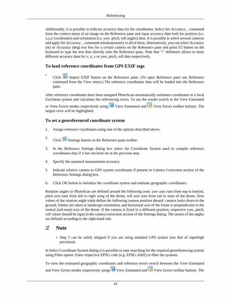
Referencing
41
Additionally, it is possible to indicate accuracy data for the coordinates. Select Set Accuracy... commandfrom the context menu of an image on the Reference pane and input accuracy data both for position (i.e.x,y,z coordinates) and orientation (i.e. yaw, pitch, roll angles) data. It is possible to select several camerasand apply Set Accuracy... command simultaneousely to all of them. Alternatively, you can select Accuracy(m) or Accuracy (deg) text box for a certain camera on the Reference pane and press F2 button on thekeyboard to type the text data directly onto the Reference pane. Note that "/" delimeter allows to enterdifferent accuracy data for x, y, z or yaw, pitch, roll data respectively.
To load reference coordinates from GPS EXIF tags
•Click Import EXIF button on the Reference pane. (To open Reference pane use Referencecommand from the View menu.) The reference coordinates data will be loaded into the Referencepane.
After reference coordinates have been assigned PhotoScan automatically estimates coordinates in a localEuclidean system and calculates the referencing errors. To see the results switch to the View Estimated
or View Errors modes respectively using View Estimated and View Errors toolbar buttons. Thelargest error will be highlighted.
To set a georeferenced coordinate system
1. Assign reference coordinates using one of the options described above.
2.Click Settings button on the Reference pane toolbar.
3. In the Reference Settings dialog box select the Coordinate System used to compile referencecoordinates data if it has not been set at the previous step.
4. Specify the assumed measurement accuracy.
5. Indicate relative camera to GPS system coordinates if present in Camera Correction section of theReference Settings dialog box.
6. Click OK button to initialize the coordinate system and estimate geographic coordinates.
Rotation angles in PhotoScan are defined around the following axes: yaw axis runs from top to bottom,pitch axis runs from left to right wing of the drone, roll axis runs from tail to nose of the drone. Zerovalues of the rotation angle triple define the following camera position aboard: camera looks down to theground, frames are taken in landscape orientation, and horizontal axis of the frame is perpendicular to thecentral (tail-nose) axis of the drone. If the camera is fixed in a different position, respective yaw, pitch,roll values should be input in the camera correction section of the Settings dialog. The senses of the anglesare defined according to the right-hand rule.
Note
• Step 5 can be safely skipped if you are using standard GPS system (not that of superhighprecision).
In Select Coordinate System dialog it is possible to ease searching for the required georeferencing systemusing Filter option. Enter respective EPSG code (e.g. EPSG::4302) to filter the systems.
To view the estimated geographic coordinates and reference errors switch between the View Estimated
and View Errors modes respectively using View Estimated and View Errors toolbar buttons. The
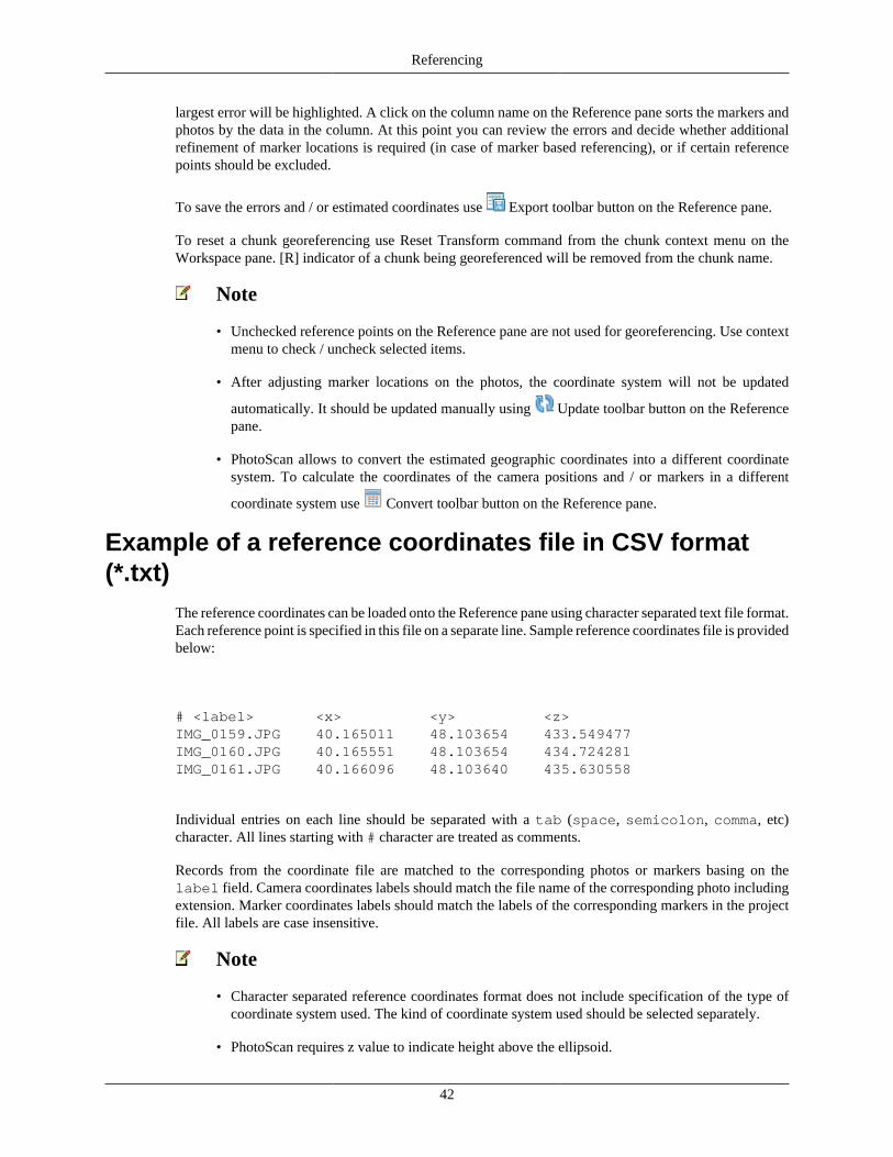
Referencing
42
largest error will be highlighted. A click on the column name on the Reference pane sorts the markers andphotos by the data in the column. At this point you can review the errors and decide whether additionalrefinement of marker locations is required (in case of marker based referencing), or if certain referencepoints should be excluded.
To save the errors and / or estimated coordinates use Export toolbar button on the Reference pane.
To reset a chunk georeferencing use Reset Transform command from the chunk context menu on theWorkspace pane. [R] indicator of a chunk being georeferenced will be removed from the chunk name.
Note
• Unchecked reference points on the Reference pane are not used for georeferencing. Use contextmenu to check / uncheck selected items.
• After adjusting marker locations on the photos, the coordinate system will not be updated
automatically. It should be updated manually using Update toolbar button on the Referencepane.
• PhotoScan allows to convert the estimated geographic coordinates into a different coordinatesystem. To calculate the coordinates of the camera positions and / or markers in a different
coordinate system use Convert toolbar button on the Reference pane.
Example of a reference coordinates file in CSV format(*.txt)
The reference coordinates can be loaded onto the Reference pane using character separated text file format.Each reference point is specified in this file on a separate line. Sample reference coordinates file is providedbelow:
# <label> <x> <y> <z>IMG_0159.JPG 40.165011 48.103654 433.549477IMG_0160.JPG 40.165551 48.103654 434.724281IMG_0161.JPG 40.166096 48.103640 435.630558
Individual entries on each line should be separated with a tab (space, semicolon, comma, etc)character. All lines starting with # character are treated as comments.
Records from the coordinate file are matched to the corresponding photos or markers basing on thelabel field. Camera coordinates labels should match the file name of the corresponding photo includingextension. Marker coordinates labels should match the labels of the corresponding markers in the projectfile. All labels are case insensitive.
Note
• Character separated reference coordinates format does not include specification of the type ofcoordinate system used. The kind of coordinate system used should be selected separately.
• PhotoScan requires z value to indicate height above the ellipsoid.
Referencing
43
Using different vertical datumsOn default PhotoScan requires all the source altitude values for both cameras and markers to be input asvalues mesuared above the ellipsoid. However, PhotoScan allows for the different geoid models utilizationas well. PhotoScan installation package includes only EGM96 geoid model, but additional geoid modelscan be downloaded from Agisoft's website if they are required by the coordinate system selected inthe Reference pane settings dialog; alternatively, a geoid model can be loaded from a custom PRJ file.Downloaded geoid model from the supported list should be copied to \geoids\ folder in PhotoScaninstallation directory before using the corresponding coordinate system from GUI.
Please refer to the following web-page to review the list of supported geoid models: http://www.agisoft.com/downloads/geoids/.
Optimization
Optimization of camera alignmentPhotoScan estimates internal and external camera orientation parameters during photo alignment. Thisestimation is performed using image data alone, and there may be some errors in the final estimates. Theaccuracy of the final estimates depends on many factors, like overlap between the neighboring photos, aswell as on the shape of the object surface. These errors can lead to non-linear deformations of the finalmodel.
During georeferencing the model is linearly transformed using 7 parameter similarity transformation (3parameters for translation, 3 for rotation and 1 for scaling). Such transformation can compensate only alinear model misalignment. The non-linear component can not be removed with this approach. This isusually the main reason for georeferencing errors.
Possible non-linear deformations of the model can be removed by optimizing the estimated point cloudand camera parameters based on the known reference coordinates. During this optimization PhotoScanadjusts estimated point coordinates and camera parameters minimizing the sum of reprojection error andreference coordinate misalignment error.
To achieve greater optimizing results it may be useful to edit sparse point cloud deleting obviouslymislocated points beforehand. To read about point cloud editing refer to the Editing point cloud sectionof the manual.
Georeferencing accuracy can be improved significantly after optimization. It is recommended to performoptimization if the final model is to be used for any kind of measurements.
To optimize camera alignment
1. Set the marker and/or camera coordinates to be used for optimization (if not done yet).
2.Click Settings toolbar button on the Reference pane and set the coordinate system (if not done yet).
3. In the Reference pane Settings dialog box specify the assumed accuracy of measured values as wellas the assumed accuracy of marker projections on the source photos.
4. Click OK button.
5. Indicate relative GPS device and/or INS to camera coordinates (if info is available) on GPS/INS tabof Camera Calibration dialog available from Tools menu.
Referencing
44
6. Check Fix GPS/INS offset box.
7. Click OK button.
8.Click Optimize toolbar button. In Optimize Camera Alignment dialog box check additionalcamera parameters to be optimized if needed. Click OK button to start optimization.
9. After the optimization is complete, the georeferencing errors will be updated.
Note
• Step 5 can be safely skipped if you are using standard GPS (not that of extremely high precision).
• Tangential distortion parameters p3, p4, are available for optimization only if p1, p2 values arenot equal to zero after alignment step.
• The model data (if any) is cleared by the optimization procedure. You will have to rebuild themodel geometry after optimization.
Image coordinates accuracy for markers indicates how precisely the markers were placed by the user oradjusted by the user after being automatically placed by the program.
Ground altitude parameter is used to make reference preselection mode of alignment procedure workeffectively for oblique imagery. See Aligning photos for details.
Camera, marker and scale bar accuracy can be set per item (i.d. per camera/marker/scale bar) usingAccuracy column on the Reference pane. Accuracy values can be typed in on the pane per item or for agroup of selected items. Alternatively accuracy values can be uploaded along with camera/marker dataas a text file (see Assigning reference coordinates subsection of Setting coordinate system). Additionally,different accuracies per coordinate can be indicated using "/" as a separator between values in the Accuracycolumn.
GPS/INS offset values input by the user can also be adjusted by PhotoScan with respect to measurementaccuracy that may be indicated on the GPS/INS tab of Camera Calibration dialog. Uncheck Fix GPS/INSoffset box to allow for adjustment procedure.
Generally it is reasonable to run optimization procedure based on markers data only. It is due to the fact thatGCPs coordinates are measured with significantly higher accuracy compared to GPS data that indicatescamera positions. Thus, markers data are sure to give more precise optimization results. Moreover, quiteoften GCP and camera coordinates are measured in different coordinate systems, that also prevents fromusing both cameras and markers data in optimization simultaneously.
The results of the optimization procedure can be evaluated with the help of error information on theReference pane. In addition, distortion plot can be inspected along with mean residuals visualised percalibration group. This data is available from Camera Calibration dialog (Tools menu), from context menuof a camera group - Distortion Plot... command. Note that residuals are averaged per cell of an imageand then across all the images in a camera group. Scale reference under the plot indicates the scale of thedistortions/residuals.
In case optimization results does not seem to be satisfactory, you can try recalculating with lower valuesof parameters, i.e. assuming ground control measurements to be more accurate.
Scale bar based optimization
Scale bar is program representation of any known distance within the scene. It can be a standard ruler ora specially prepared bar of a known length. Scale bar is a handy tool to add supportive reference data to
Referencing
45
your project. They can prove to be useful when there is no way to locate ground control points all overthe scene. Scale bars allow to save field work time, since it is significantly easier to place several scalebars with precisely known length, then to measure coordinates of a few markers using special equipment.In addition, PhotoScan allows to place scale bar instances between cameras, thus making it possible toavoid not only marker but ruler placement within the scene as well. Surely, scale bar based informationwill not be enough to set a coordinate system, however, the information can be successfully used whileoptimizing the results of photo alignment. It will also be enough to perform measurements in PhotoScansoftware. See Performing measurements on mesh.
To add a scale bar
1. Place markers at the start and end points of the bar. For information on marker placement please referto the Setting coordinate system section of the manual.
2. Select both markers on the Reference pane using Ctrl button.
3.Select Create Scale Bar command form the Model view context menu. The scale bar will becreated and an instant added to the Scale Bar list on the Reference pane.
4.Switch to the View Source mode using the Reference pane toolbar button.
5. Double click on the Distance (m) box next to the newly created scale bar name and enter the knownlength of the bar in meters.
To add a scale bar between cameras
1. Select the two cameras on the Workspace or Reference pane using Ctrl button. Alternatively, thecameras can be selected in the Model view window using selecting tools from the Toolbar.
2.Select Create Scale Bar command form the context menu. The scale bar will be created and aninstant added to the Scale Bar list on the Reference pane.
3.Switch to the View Source mode using the Reference pane toolbar button.
4. Double click on the Distance (m) box next to the newly created scale bar name and enter the knownlength of the bar in meters.
To run scale bar based optimization
1. On the Reference pane check all scale bars to be used in optimization procedure.
2.Click Settings toolbar button on the Reference pane. In the Reference pane Settings dialog boxspecify the assumed accuracy of scale bars measurements.
3. Click OK button.
4.Click Optimize toolbar button. In Optimize Camera Alignment dialog box check additionalcamera parameters to be optimized if needed. Click OK button to start optimization.
After the optimization is complete, cameras and markers estimated coordinates will be updated as well asall the georeferencing errors. To analyze optimization results switch to the View Estimated mode usingthe Reference pane toolbar button. In scale bar section of the Reference pane estimated scale bar distancewill be displayed.
Referencing
46
To delete a scale bar
1. Select the scale bar to be deleted on the Reference pane.
2. Right-click on it and chose Remove Scale Bars command from the context menu.
3. Click OK for the selected scale bar to be deleted.
What do the errors in the Reference pane mean?
Cameras section
1. Error (m) - distance between the input (source) and estimated positions of the camera.
2. Error (deg) - root mean square error calculated over all three orientation angles.
3. Error (pix) - root mean square reprojection error calculated over all feature points detected on thephoto.
Reprojection error is the distance between the point on the image where a reconstructed 3D point can beprojected and the original projection of that 3D point detected on the photo and used as a basis for the3D point reconstruction procedure.
Markers section
1. Error (m) - distance between the input (source) and estimated positions of the marker.
2. Error (pix) - root mean square reprojection error for the marker calculated over all photos wheremarker is visible.
Scale Bars section
• Error (m) - difference between the input (source) scale bar length and the measured distance betweentwo cameras or markers representing start and end points of the scale bar.
If the total reprojection error for some marker seems to be too large, it is recommended to inspectreprojection errors for the marker on individual photos. The information is available with Show Infocommand from the marker context menu on the Reference pane.
Working with coded and non-coded targets
OverviewCoded and non-coded targets are specially prepared, yet quite simple, real world markers that can add upto successful 3D model reconstruction of a scene. The difference between coded and non-coded targetsis that while a non-coded target looks like an ordinary full circle or a figure (circle / rectangular) with 4segments, the coded target has a ring parted in black and white segments around the central full circle.
Coded targets advantages and limitationsCoded targets (CTs) can be used as markers to define local coordinate system and scale of the model or astrue matches to improve photo alignment procedure. PhotoScan functionality includes automatic detectionand matching of CTs on source photos, which allows to benefit from marker implementation in the project
Referencing
47
while saving time on manual marker placement. Moreover, automatic CTs detection and marker placementis more precise then manual marker placement.
PhotoScan supports three types of circle CTs: 12 bit, 16 bit and 20 bit. While 12 bit pattern is consideredto be decoded more precisely, 16 bit and 20 bit patterns allow for a greater number of CTs to be usedwithin the same project.
To be detected successfully CTs must take up a significant number of pixels on the original photos. Thisleads to a natural limitation of CTs implementation: while they generally prove to be useful in close-rangeimagery projects, aerial photography projects will demand too huge CTs to be placed on the ground, forthe CTs to be detected correctly.
Coded targets in workflowSets of all patterns of CTs supported by PhotoScan can be generated by the program itself.
To create a printable PDF with coded targets
1. Select Print Markers... command from the Tools menu.
2. Specify the CTs type and desired print parameters in Print Markers dialog.
3. Click OK.
Once generated, the pattern set can be printed and the CTs can be placed over the scene to be shot andreconstructed.
When the images with CTs seen on them are uploaded to the program, PhotoScan can detect and matchthe CTs automatically.
To detect coded targets on source images
1. Select Detect Markers... command from the Tools menu.
2. Specify parameters of detector in Detect Markers dialog according to the CTs type.
3. Click OK.
PhotoScan will detect and match CTs and add corresponding markers to the Reference pane.
CTs generated with PhotoScan software contain even number of sectors. However, previous versions ofPhotoScan software had no restriction of the kind. Thus, if the project to be processed contains CTs fromprevious versions of PhotoScan software, it is required to disable parity check in order to make the detectorwork.
Non-coded targets implementationNon-coded targets can also be automatically detected by PhotoScan (see Detect Markers dialog) . However,for non-coded targets to be matched automatically, it is necessary to run align photos procedure first.
Non-coded targets are more appropriate for aerial surveying projects due to the simplicity of the patternto be printed on a large scale. But, looking alike, they does not allow for automatic identification, somanual assignment of an identifier is required if some referencing coordinates are to be imported froma file correctly.
48
Chapter 5. MeasurementsPerforming measurements on mesh
PhotoScan supports measuring of distances between control points, as well as of surface area and volumeof the reconstructed 3D model.
Distance measurementPhotoScan enables measurements of direct distances between the points of the reconstructed 3D scene. Thepoints used for distance measurement must be defined by placing markers in the corresponding locations.Model coordinate system must be also initialized before the distance measurements can be performed.Alternatively, the model can be scaled based on known distance (scale bar) information to become suitablefor measurements.
For instructions on placing markers, refining their positions and setting coordinate system please refer tothe Setting coordinate system section of the manual. Scale bar concept is described in the Optimizationsection.
To measure distance
1. Place the markers in the scene at the locations to be used for distance measurement. For informationon marker placement please refer to the Setting coordinate system section of the manual.
2. Select both markers to be used for distance measurements on the Reference pane using Ctrl button.
3.Select Create Scale Bar command form the 3D view context menu. The scale bar will be createdand an instant added to the Scale Bar list on the Reference pane.
4.Switch to the estimated values mode using View Estimated button from the Reference panetoolbar.
5. The estimated distance for the newly created scale bar equals to the distance that should have beenmeasured.
To measure distance between cameras
1. Select the two cameras on the Workspace or Reference pane using Ctrl button. Alternatively, thecameras can be selected in the Model view window using selecting tools from the Toolbar.
2.Select Create Scale Bar command form the context menu. The scale bar will be created and aninstant added to the Scale Bar list on the Reference pane.
3.Switch to the estimated values mode using View Estimated button from the Reference panetoolbar.
4. The estimated distance for the newly created scale bar equals to the distance that should have beenmeasured.
Note
• Please note that the scale bar used for distance measurements must be unchecked on theReference pane.
Measurements
49
Note
• The distance values measured by PhotoScan are displayed in meters.
Surface area and volume measurementSurface area or volume measurements of the reconstructed 3D model can be performed only after the scaleor coordinate system of the scene is defined. For instructions on setting coordinate system please refer tothe Setting coordinate system section of the manual.
To measure surface area and volume
1. Select Measure Area and Volume... command from the Tools menu.
2. The whole model surface area and volume will be displayed in the Measure Area and Volume dialogbox. Surface area is measured in square meters, while mesh volume is measured in cubic meters.
Volume measurement can be performed only for the models with closed geometry. If there are any holesin the model surface PhotoScan will report zero volume. Existing holes in the mesh surface can be filledin before performing volume measurements using Close Holes... command from the Tools menu.
Performing measurements on DEMPhotoScan is capable of DEM-based point, distance, area, and volume measurements as well as ofgenerating cross-sections for a part of the scene selected by the user. Additionally, contour lines can becalculated for the model and depicted either over DEM or Orthomosaic in Ortho view within PhotoScanenvironment. Measurements on the DEM are controlled with shapes: points, polylines and polygons.
ShapesShapes are used to indicate boundaries either for DEM/Orthomosaic export or for the measurementprocedures. Shapes can be drawn over DEM or Orthomosaic using buttons from the Ortho view toolbar.Alternatively, shapes can be loaded from a .SHP file using Import Shapes... subcommand of Import...command available from the Tools menu. Shapes created in PhotoScan can be exported using ExportShapes... subcommand of Export... command available from the Tools menu
To draw a shape
1. Open DEM/orthomosaic in Ortho view double clicking on DEM/orthomosaic label in the Workspacepane.
2.Select Draw Point / Draw Polyline / Draw Polygon instrument from the Ortho view toolbar.
3. Draw a point/polyline/polygon on the DEM/orthomosaic with a cursor.
4. Double click on the last point to indicate the end of a polyline. To complete a polygon, place the endpoint over the starting one.
5.Once the shape is drawn, a shape label will be added to the chunk data structure on the Workspacepane. All shapes drawn on the same DEM (and on the corresponding orthomosaic) will be shownunder the same label on the Workspace pane.
6. The program will switch to a navigation mode once a shape is completed.
Measurements
50
After a shape has been drawn, it can be edited using Insert Vertex / Delete Vertex commands from thecontext menu. Delete Vertex command is active only for a vertex context menu. To get access to the vertexcontext menu, select the shape with a double click first, and then select the vertex with a double click onit. To change position of a vertex, drag and drop it to a selected position with the cursor.
Point measurementOrtho view allows to measure coordinates of any point on the reconstructed model. X and Y coordinatesof the point indicated with the cursor as well as height of the point above the vertical datum selected bythe user are shown in the bottom right corner of the Ortho view.
Distance measurement
To measure distance
1.Connect the points of interest with a polyline using Draw Polyline tool from the Ortho viewtoolbar.
2. Double click on the last point to indicate the end of a polyline.
3. Right button click on the polyline and select Measure... command from the context menu.
4. In the Measure Shape dialog inspect the results. Perimeter value equals to the distance that shouldhave been measured.
In addition to polyline length value (see perimeter value in the Measure Shape), coordinates of the verticesof the polyline are shown on the Planar tab of the Measure Shape dialog.
Note
• Measure option is available from the context menu of a selected polyline. To select a polyline,double-click on it. A selected polyline is coloured in red.
Surface area and volume measurement
To measure area and volume
1.Draw a polygon on the DEM using Draw Polygon instrument to indicate the area to be measured.
2. Right button click on the polygon and select Measure... command from the context menu.
3. In the Measure Shape dialog inspect the results: see area value on the Planar tab and volume valueson the Volume tab.
PhotoScan allows to measure volume above best fit / mean level / custom level planes. Best fit and meanlevel planes are calculated based on the drawn polygon vertices. Volume measured against custom levelplane allows to trace volume changes for the same area in the course of time.
Note
• Measure option is available from the context menu of a selected polygon. To select a polygon,double-click on it. A selected polygon is coloured in red.
Measurements
51
Cross sections and contour linesPhotoScan enables to calculate cross sections, using shapes to indicate the plane(s) for a cut(s), the cutbeing made with a plane parallel to Z axis. For a polyline/polygon the program will calculate profiles alongall the edges starting from the first drawn side.
To calculate cross section
1.Indicate a line to make a cut of the model using Draw Polyline / Draw Polygon tool from theOrtho view toolbar.
2. Double click on the last point to indicate the end of a polyline.
3. Right button click on the polyline/polygon and select Measure... command from the context menu.
4. In the Measure Shape dialog inspect the results on the Profile tab of the dialog.
Generate Contours...command is available either from DEM label context menu on the Workspace paneor from the Tools menu.
To generate contours
1. Select Generate Contours...command from Tools menu.
2. In the Generate Contours dialog select DEM as the source data for calculation.
3. Set values for Minimal altitude, Maximal altitude parameters as well as the Interval for the contours.All the values shoudl be indicated in meters.
4. Click OK button once done.
5. The progress dialog box will appear displaying the current processing status. To cancel processingclick Cancel button.
6. When the procedure is finished, a contour lines label will be added to the project file structure shownon the Workspace pane.
Contour lines can be shown over the DEM or orthomosaic on the Ortho tab of the program window. Use
Show contour lines tool from the Ortho tab toolbal to switch the function on and off. Contour lines canbe deleted using Remove Contours command from the contour lines label context menu on the Workspacepane.
Contour lines can be exported using Export Contours command from the contour lines label context menuon the Workspace pane. Alternatively the command is available from the Tools menu. In the ExportContour Lines dialog it is necessary to select the type of the contour lines to be exported. A .SHP file canstore the lines of the same type only: either polygons or polylines.
Vegetation indices calculationPhotoScan enables to calculate NDVI and other vegetation indices based on the multispectral imageryinput. A vegetation index formula can be set by the user, thus allowing for great flexibility in data analysis.Calculated data can be exported as a grid of floating point index values calculated per pixel of orthomosaicor as an orthomosaic in pseudocolors according to a pallet set by the user.
Measurements
52
To calculate a vegetation index
1. Open orthomosaic in the Ortho tab doubleclicking on the orthomosaic label on the Workspace pane.
2.Open Raster Calculator tool using Raster Calculator button from the Ortho view toolbar.
3. Input an index expression using keyboard input and operators buttons of the raster calculator ifnecessary.
4. Check Enable transform box and press OK button to calculate index values.
5. Once the operation is completed, the result will be shown in the Ortho view, index values beingvisualised with colours according to the palette set in the Raster Calculator dialog.
Palette defines the colour for each index value to be shown with. PhotoScan offers several standard palettepresets on the Palette tab of the Raster Calculator dialog. A preset (NDVI, Heat, Gray scale) can be chosenfrom a drop-down list. Alternatively, the user can upload the palette from a Surfer Color Spectrum (*.clr)
file ( Import Palette), preliminary prepared in an external tool. The palette can also be edited within
PhotoScan environment using Add Color and Remove Color buttons on the Palette tab of the RasterCalculator dialog. For each new line added to the palette a certain index value should be typed in. Doubleclick on the newly added line to type the value in. A customised palette can be saved for future projects
using Export Palette button on the Palette tab of the Raster Calculator dialog.
PhotoScan enables to calculate contour lines based on the calculated index values.
To calculate contour lines based on vegetation index data
1. Select Generate Contours... command from the orthomosaic icon context menu on the Workspacepane, while index data is shown in the Ortho view.
2. Select Orthomosaic as the source for the contours calculation.
3. Adjust the min/max value and the interval parameters for the task.
4. Press OK button to calculate index values.
5. The progress dialog box will appear displaying the current processing status. To cancel processingclick Cancel button.
6. When the procedure is finished, a contour lines label will be added to the project file structure shownon the Workspace pane. The contour lines will be shown over the index data on the Ortho tab.
Note
• PhotoScan keeps only the latest contour lines data calculated. Thus, if you need to save contourlines calculated for the DEM data, use Export Contours... command from the contour lines labelcontext menu on the Workspace pane before generating contour lines for the index data.
After vegetation index results having been inspected, the original orthomosaic can be opened withunchecking Enable transform box in the Raster Calculator and pressing OK button.
Index data can be saved with Export orthomosaic command from the File menu. For guidance on the exportprocedure, please refer to NDVI data export section of the manual.
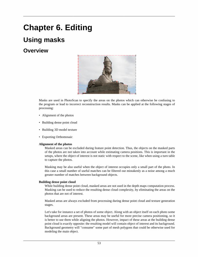
53
Chapter 6. EditingUsing masks
Overview
Masks are used in PhotoScan to specify the areas on the photos which can otherwise be confusing tothe program or lead to incorrect reconstruction results. Masks can be applied at the following stages ofprocessing:
• Alignment of the photos
• Building dense point cloud
• Building 3D model texture
• Exporting Orthomosaic
Alignment of the photosMasked areas can be excluded during feature point detection. Thus, the objects on the masked partsof the photos are not taken into account while estimating camera positions. This is important in thesetups, where the object of interest is not static with respect to the scene, like when using a turn tableto capture the photos.
Masking may be also useful when the object of interest occupies only a small part of the photo. Inthis case a small number of useful matches can be filtered out mistakenly as a noise among a muchgreater number of matches between background objects.
Building dense point cloudWhile building dense point cloud, masked areas are not used in the depth maps computation process.Masking can be used to reduce the resulting dense cloud complexity, by eliminating the areas on thephotos that are not of interest.
Masked areas are always excluded from processing during dense point cloud and texture generationstages.
Let's take for instance a set of photos of some object. Along with an object itself on each photo somebackground areas are present. These areas may be useful for more precise camera positioning, so itis better to use them while aligning the photos. However, impact of these areas at the building densepoint cloud is exactly opposite: the resulting model will contain object of interest and its background.Background geometry will "consume" some part of mesh polygons that could be otherwise used formodeling the main object.
Editing
54
Setting the masks for such background areas allows to avoid this problem and increases the precisionand quality of geometry reconstruction.
Building texture atlasDuring texture atlas generation, masked areas on the photos are not used for texturing. Masking areason the photos that are occluded by outliers or obstacles helps to prevent the "ghosting" effect on theresulting texture atlas.
Loading masksMasks can be loaded from external sources, as well as generated automatically from background imagesif such data is available. PhotoScan supports loading masks from the following sources:
• From alpha channel of the source photos.
• From separate images.
• Generated from background photos based on background differencing technique.
• Based on reconstructed 3D model.
To import masks
1. Select Import Masks... command from the Tools menu.
2. In the Import Mask dialog select suitable parameters. Click OK button when done.
3. When generating masks from separate or background images, the folder selection dialog will appear.Browse to the folder containing corresponding images and select it.
4. The progress dialog box will appear displaying the current processing status. To cancel processingclick Cancel button.
The following parameters can be specified during mask import:
Import masks forSpecifies whether masks should be imported for the currently opened photo, active chunk or entireWorkspace.
Current photo - load mask for the currently opened photo (if any).
Active chunk - load masks for active chunk.
Entire workspace - load masks for all chunks in the project.
MethodSpecifies the source of the mask data.
From Alpha - load masks from alpha channel of the source photos.
From File - load masks from separate images.
From Background - generate masks from background photos.
From Model - generate masks based on reconstructed model.

Editing
55
Mask file names (not used in From alpha mode)Specifies the file name template used to generate mask file names. This template can contain specialtokens, that will be substituted by corresponding data for each photo being processed. The followingtokens are supported:
{filename} - file name of the source photo without extension.
{fileext} - extension of the source photo.
{camera} - camera label.
{frame} - frame number.
{filenum} - sequential number of the mask being imported.
For example, {filename}_mask.png template can be used if masks are available in PNG format andhave a _mask suffix.
Tolerance (From Background method only)Specifies the tolerance threshold used for background differencing. Tolerance value should be setaccording to the color separation between foreground and background pixels. For larger separationhigher tolerance values can be used.
Editing masksModification of the current mask is performed by adding or subtracting selections. A selection is createdwith one of the supported selection tools and is not incorporated in the current mask until it is merged witha mask using Add Selection or Subtract Selection operations.
To edit the mask
1. Open the photo to be masked by double clicking on its name on the Workspace / Photo pane. Thephoto will be opened in the main window. The existing mask will be displayed as a shaded regionon the photo.
2. Select the desired selection tool and generate a selection.
3.Click on Add Selection toolbar button to add current selection to the mask, or Subtract
Selection to subtract the selection from the mask. Invert Selection button allows to invert currentselection prior to adding or subtracting it from the mask.
The following tools can be used for creating selections:
Rectangle selection toolRectangle selection tool is used to select large areas or to clean up the mask after other selection toolswere applied.
Intelligent scissors toolIntelligent scissors is used to generate a selection by specifying its boundary. The boundary is formedby selecting a sequence of vertices with a mouse, which are automatically connected with segments.The segments can be formed either by straight lines, or by curved contours snapped to the objectboundaries. To enable snapping, hold Ctrl key while selecting the next vertex. To complete theselection, the boundary should be closed by clicking on the first boundary vertex.
Editing
56
Intelligent paint toolIntelligent paint tool is used to "paint" a selection by the mouse, continuously adding small imageregions, bounded by object boundaries.
Magic wand toolMagic Wand tool is used to select uniform areas of the image. To make a selection with a MagicWand tool, click inside the region to be selected.
The range of pixel colors selected by Magic Wand is controlled by the tolerance value. At lowertolerance values the tool selects fewer colors similar to the pixel you click with the Magic Wand tool.Higher value broadens the range of colors selected.
Note
• To add new area to the current selection hold the Ctrl key during selection of additional area.
• To reset mask selection on the current photo press Esc key.
A mask can be inverted using Invert Mask command from the Photo menu. The command is active inPhoto View only. Alternatively, you can invert masks either for selected cameras or for all cameras in achunk using Invert Masks... command from a photo context menu on the Photos pane.
The masks are generated individually for each image. If some object should be masked out, it should bemasked out on all photos, where that object appears.
Saving masksCreated masks can be also saved for external editing or storage.
To export masks
1. Select Export Masks... command from the Tools menu.
2. In the Export Mask dialog select suitable parameters. Click OK button when done.
3. Browse to the folder where the masks should be saved and select it.
4. The progress dialog box will appear displaying the current processing status. To cancel processingclick Cancel button.
The following parameters can be specified during mask export:
Export masks forSpecifies whether masks should be exported for the currently opened photo, active chunk or entireWorkspace.
Current photo - save mask for the currently opened photo (if any).
Active chunk - save masks for active chunk.
Entire workspace - save masks for all chunks in the project.
File typeSpecifies the type of generated files.
Editing
57
Single channel mask image - generates single channel black and white mask images.
Image with alpha channel - generates color images from source photos combined with maskdata in alpha channel.
Mask file namesSpecifies the file name template used to generate mask file names. This template can contain specialtokens, that will be substituted by corresponding data for each photo being processed. The followingtokens are supported:
{filename} - file name of the source photo without extension.
{fileext} - extension of the source photo.
{camera} - camera label.
{frame} - frame number.
{filenum} - sequential number of the mask being exported.
For example, {filename}_mask.png template can be used to export masks in PNG format with _masksuffix.
Note
• When importing/exporting mask for the current photo only, PhotoScan will prompt for the actualimage instead of image folder. Mask file names parameter will not be used in this case.
Editing point cloudThe following point cloud editing tools are available in PhotoScan:
• Automatic filtering based on specified criterion (sparse cloud only)
• Automatic filtering based on applied masks (dense cloud only)
• Automatic filtering based on points colours (dense cloud only)
• Reducing number of points in cloud by setting tie point per photo limit (sparse cloud only)
• Manual points removal
Note
• Point cloud editing operation can be undone/redone using Undo/Redo command from the Editmenu.
Filtering points based on specified criterionIn some cases it may be useful to find out where the points with high reprojection error are located withinthe sparse cloud, or remove points representing high amount of noise. Point cloud filtering helps to selectsuch points, which usually are supposed to be removed.
PhotoScan supports the following criteria for point cloud filtering:

Editing
58
Reprojection errorHigh reprojection error usually indicates poor localization accuracy of the corresponding pointprojections at the point matching step. It is also typical for false matches. Removing such points canimprove accuracy of the subsequent optimization step.
Reconstruction uncertaintyHigh reconstruction uncertainty is typical for points, reconstructed from nearby photos with smallbaseline. Such points can noticeably deviate from the object surface, introducing noise in the pointcloud. While removal of such points should not affect the accuracy of optimization, it may be usefulto remove them before building geometry in Point Cloud mode or for better visual appearance of thepoint cloud.
Image countPhotoScan reconstruct all the points that are visible at least on two photos. However, points that arevisible only on two photos are likely to be located with poor accuracy. Image count filtering enablesto remove such unreliable points from the cloud.
Projection AccuracyThis criterion allows to filter out points which projections were relatively poorer localised due to theirbigger size.
To remove points based on specified criterion
1.Switch to Point Cloud view mode using Point Cloud toolbar button.
2. Select Gradual Selection... command from the Edit menu.
3. In the Gradual Selection dialog box specify the criterion to be used for filtering. Adjust the thresholdlevel using the slider. You can observe how the selection changes while dragging the slider. ClickOK button to finalize the selection.
4.To remove selected points use Delete Selection command from the Edit menu or click DeleteSelection toolbar button (or simply press Del button on the keyboard).
Filtering points based on applied masks
To remove points based on applied masks
1.Switch to Dense Cloud view mode using Dense Cloud toolbar button.
2. Choose Select Masked Points... command from the Dense Cloud submenu of the Tools menu.
3. In the Select Masked Points dialog box indicate the photos whose masks to be taken into account.Adjust the edge softness level using the slider. Click OK button to run the selection procedure.
4.To remove selected points use Delete Selection command from the Edit menu or click DeleteSelection toolbar button (or simply press Del button on the keyboard).
Filtering points based on points colors
To remove points based on points colors
1.Switch to Dense Cloud view mode using Dense Cloud toolbar button.
Editing
59
2. Choose Select Points by Color... command from the Dense Cloud submenu of the Tools menu.
3. In the Select Points by Color dialog box the color to be used as the criterion. Adjust the tolerancelevel using the slider. Click OK button to run the selection procedure.
4.To remove selected points use Delete Selection command from the Edit menu or click DeleteSelection toolbar button (or simply press Del button on the keyboard).
Tie point per photo limitTie point limit parameter could be adjusted before Align photos procedure. The number indicates the upperlimit for matching points for every image. Using zero value doesn't apply any tie-point filtering.
The number of tie points can also be reduced after the alignment process with Tie Points - Thin Point Cloudcommand available from Tools menu. As a results sparse point cloud will be thinned, yet the alignmentwill be kept unchanged.
Manual points removalIncorrect points can be also removed manually.
To remove points from a point cloud manually
1.Switch to Sparse Cloud view mode using Point Cloud toolbar button or to Dense Cloud view
mode using Dense Cloud toolbar button.
2.Select points to be removed using Rectangle Selection, Circle Selection or Free-FormSelection tools. To add new points to the current selection hold the Ctrl key during selection ofadditional points. To remove some points from the current selection hold the Shift key duringselection of points to be removed.
3.To delete selected points click the Delete Selection toolbar button or select Delete Selection
command from the Edit menu. To crop selection to the selected points click the Crop Selectiontoolbar button or select Crop Selection command from the Edit menu.
Classifying dense cloud pointsPhotoScan allows not only to generate and visualize dense point cloud but also to classify the points withinit. There are two options: automatic division of all the points into two classes - ground points and the rest,and manual selection of a group of points to be placed in a certain class from the standard list known forLIDAR data. Dense cloud points classification opens way to customize Build Mesh step: you can choosewhat type of objects within the scene you would like to be reconstructed and indicate the correspondingpoint class as a source data for mesh generation. For example, if you build mesh or DEM based on groundpoints only, it will be possible to export DTM (as opposed to DSM) at the next step.
Automatic classification of ground pointsFor the user to avoid extra manual work PhotoScan offers feature for automatic detection of ground points.

Editing
60
To classify ground points automatically
1. Select Classify Ground Points... command from the Dense Cloud submenu of the Tools menu.
2. In the Classify Ground Points dialog box select the source point data for the classification procedure.Click OK button to run the classification procedure.
Automatic classification procedure consists of two steps. At the first step the dense cloud is divided intocells of a certain size. In each cell the lowest point is detected. Triangulation of these points gives the firstapproximation of the terrain model.
At the second step new point is added to the ground class, providing that it satisfies two conditions: it lieswithin a certain distance from the terrain model and that the angle between terrain model and the line toconnect this new point with a point from a ground class is less than a certain angle. The second step isrepeated while there still are points to be checked.
The following parameters control automatic ground points classification procedure
Max angle (deg)Determines one of the conditions to be checked while testing a point as a ground one, i.e. sets limitationfor an angle between terrain model and the line to connect the point in question with a point from aground class. For nearly flat terrain it is recommended to use default value of 15 deg for the parameter.It is reasonable to set a higher value, if the terrain contains steep slopes.
Max distance (m)Determines one of the conditions to be checked while testing a point as a ground one, i.e. sets limitationfor a distance between the point in question and terrain model. In fact, this parameter determines theassumption for the maximum variation of the ground elevation at a time.
Cell size (m)Determines the size of the cells for point cloud to be divided into as a preparatory step in groundpoints classification procedure. Cell size should be indicated with respect to the size of the largestarea within the scene that does not contain any ground points, e. g. building or close forest.
Manual classification of dense cloud pointsPhotoScan allows to associate all the points within the dense cloud with a certain standard class (seeLIDAR data classification). This provides possibility to diversify export of the processing results withrespect to different types of objects within the scene, e. g. DTM for ground, mesh for buildings and pointcloud for vegetation.
To assign a class to a group of points
1.Switch to Dense Cloud view mode using using Dense Cloud toolbar button.
2.Select points to be placed to a certain class using Rectangle Selection, Circle Selection or
Free-Form Selection tools. To add new points to the current selection hold the Ctrl key duringselection of additional points. To remove some points from the current selection hold the Shift keyduring selection of points to be removed.
3. Select Assign Class... command from the Dense Cloud submenu of the Tools menu.
4. In the Assign Class dialog box select the source point data for the classification procedure and thetargeted class to be assigned to the selected points. Click OK button to run classification procedure.
Editing
61
Dense point cloud classification can be reset with Reset Classification command from Tools - Dense Cloudmenu.
Editing model geometryThe following mesh editing tools are available in PhotoScan:
• Decimation tool
• Close Holes tool
• Automatic filtering based on specified criterion
• Manual polygon removal
• Fixing mesh topology
More complex editing can be done in the external 3D editing tools. PhotoScan allows to export mesh andthen import it back for this purpose.
Note
• For polygon removal operations such as manual removal and connected component filtering itis possible to undo the last mesh editing operation. There are Undo/Redo commands in the Editmenu.
• Please note that undo/redo commands are not supported for mesh decimation and this operationcannot be undone.
Decimation toolDecimation is a tool used to decrease the geometric resolution of the model by replacing high resolutionmesh with a lower resolution one, which is still capable of representing the object geometry with highaccuracy. PhotoScan tends to produce 3D models with excessive geometry resolution, so mesh decimationis usually a desirable step after geometry computation.
Highly detailed models may contain hundreds of thousands polygons. While it is acceptable to work withsuch a complex models in 3D editor tools, in most conventional tools like Adobe Reader or Google Earthhigh complexity of 3D models may noticeably decrease application performance. High complexity alsoresults in longer time required to build texture and to export model in pdf file format.
In some cases it is desirable to keep as much geometry details as possible like it is needed for scientific andarchive purposes. However, if there are no special requirements it is recommended to decimate the modeldown to 100 000 - 200 000 polygons for exporting in PDF, and to 100 000 or even less for displaying inGoogle Earth and alike tools.
To decimate 3D model
1. Select Decimate Mesh... command from the Tools menu.
2. In the Decimate Mesh dialog box specify the target number of polygons, which should remain in thefinal model. Click on the OK button to start decimation.
3. The progress dialog box will appear displaying the current processing status. To cancel processingclick on the Cancel button.
Editing
62
Note
• Texture atlas is discarded during decimation process. You will have to rebuild texture atlas afterdecimation is complete.
Close Holes toolClose Holes tool provides possibility to repair your model if the reconstruction procedure resulted in amesh with several holes, due to insufficient image overlap for example.
Some tasks require a continuous surface disregarding the fact of information shortage. It is necessary togenerate a close model, for instance, to fulfill volume measurement task with PhotoScan.
Close holes tool enables to close void areas on the model substituting photogrammetric reconstructionwith extrapolation data. It is possible to control an acceptable level of accuracy indicating the maximumsize of a hole to be covered with extrapolated data.
To close holes in a 3D model
1. Select Close Holes... command from the Tools menu.
2. In the Close Holes dialog box indicate the maximum size of a hole to be covered with the slider. Clickon the OK button to start the procedure.
3. The progress dialog box will appear displaying the current processing status. To cancel processingclick on the Cancel button.
Note
• The slider allows to set the size of a hole in relation to the size of the whole model surface.
Polygon filtering on specified criterionIn some cases reconstructed geometry may contain the cloud of small isolated mesh fragments surroundingthe "main" model or big unwanted polygons. Mesh filtering based on different criteria helps to selectpolygons, which usually are supposed to be removed.
PhotoScan supports the following criteria for face filtering:
Connected component sizeThis filtering criteria allows to select isolated fragments with a certain number of polygons. Thenumber of polygons in all isolated components to be selected is set with a slider and is indicated inrelation to the number of polygons in the whole model. The components are ranged in size, so thatthe selection proceeds from the smallest component to the largest one.
Polygon sizeThis filtering criteria allows to select polygons up to a certain size. The size of the polygons to beselected is set with a slider and is indicated in relation to the size of the whole model. This functioncan be useful, for example, in case the geometry was reconstructed in Smooth type and there is a needto remove extra polygons automatically added by PhotoScan to fill the gaps; these polygons are oftenof a larger size that the rest.
To remove small isolated mesh fragments
1. Select Gradual Selection... command from the Edit menu.
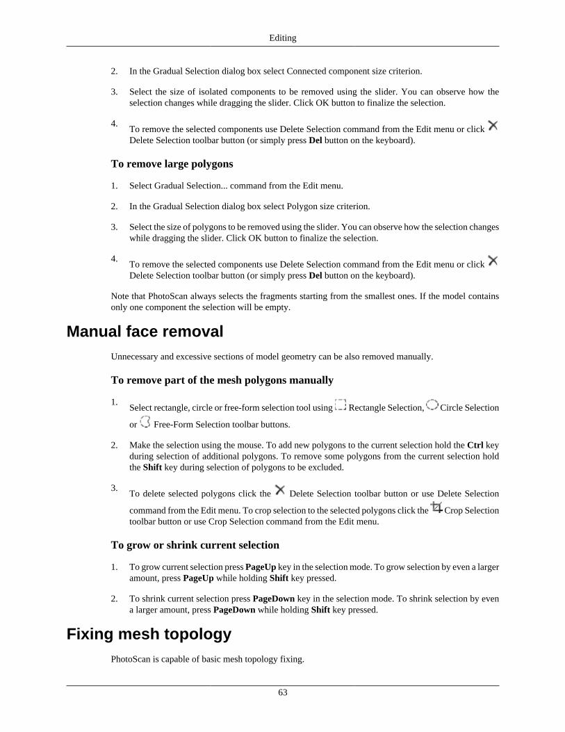
Editing
63
2. In the Gradual Selection dialog box select Connected component size criterion.
3. Select the size of isolated components to be removed using the slider. You can observe how theselection changes while dragging the slider. Click OK button to finalize the selection.
4.To remove the selected components use Delete Selection command from the Edit menu or click Delete Selection toolbar button (or simply press Del button on the keyboard).
To remove large polygons
1. Select Gradual Selection... command from the Edit menu.
2. In the Gradual Selection dialog box select Polygon size criterion.
3. Select the size of polygons to be removed using the slider. You can observe how the selection changeswhile dragging the slider. Click OK button to finalize the selection.
4.To remove the selected components use Delete Selection command from the Edit menu or click Delete Selection toolbar button (or simply press Del button on the keyboard).
Note that PhotoScan always selects the fragments starting from the smallest ones. If the model containsonly one component the selection will be empty.
Manual face removalUnnecessary and excessive sections of model geometry can be also removed manually.
To remove part of the mesh polygons manually
1.Select rectangle, circle or free-form selection tool using Rectangle Selection, Circle Selection
or Free-Form Selection toolbar buttons.
2. Make the selection using the mouse. To add new polygons to the current selection hold the Ctrl keyduring selection of additional polygons. To remove some polygons from the current selection holdthe Shift key during selection of polygons to be excluded.
3.To delete selected polygons click the Delete Selection toolbar button or use Delete Selection
command from the Edit menu. To crop selection to the selected polygons click the Crop Selectiontoolbar button or use Crop Selection command from the Edit menu.
To grow or shrink current selection
1. To grow current selection press PageUp key in the selection mode. To grow selection by even a largeramount, press PageUp while holding Shift key pressed.
2. To shrink current selection press PageDown key in the selection mode. To shrink selection by evena larger amount, press PageDown while holding Shift key pressed.
Fixing mesh topologyPhotoScan is capable of basic mesh topology fixing.
Editing
64
To fix mesh topology
1. Select View Mesh Statistics... command from the Tools menu.
2. In the Mesh Statistics dialog box you can inspect mesh parameters. If there are any topologicalproblems, Fix Topology button will be active and can be clicked to solve the problems.
3. The progress dialog box will appear displaying the current processing status. To cancel processingclick on the Cancel button.
Editing mesh in the external program
To export mesh for editing in the external program
1. Select Export Model... command from the File menu.
2. In the Save As dialog box, specify the desired mesh format in the Save as type combo box. Select thefile name to be used for the model and click Save button.
3. In the opened dialog box specify additional parameters specific to the selected file format. Click OKbutton when done.
To import edited mesh
1. Select Import Mesh... command from the Tools menu.
2. In the Open dialog box, browse to the file with the edited model and click Open.
Note
• PhotoScan supports loading models in Wavefront OBJ, 3DS, STL, COLLADA, Stanford PLY,Autodesk FBX, Autodesk DXF, OpenCTM and U3D file formats only. Please make sure to selectone of these file formats when exporting model from the external 3D editor.
• Please be aware that it is important to keep reference information for the model if any.
Orthomosaic seamlines editingPhotoScan software offers various blending options at orthomosaic generation step for the user to adjustprocessing to their data and task. However, in some projects moving objects can cause artifacts whichinterfere with visual quality of the orthomosaic. The same problem may result from oblique aerial imageryprocessing if the area of interest contains high buildings or if the user has captured facade from too obliquepositions. To eliminate mentioned artifacts PhotoScan offers seamline editing tool. The functionalityallows to choose manually the image or images to texture the indicated part of the orthomosaic from. Thus,the final orthomosaic can be improved visually according to the user's expectations.
Automatic seamlines can be turned on for inspection in the Ortho view with pressing the ShowSeamlines button from the Ortho view toolbar.
To edit orthomosaic seamlines
1.Draw a polygon on the orthomosaic using Draw Polygon instrument to indicate the area to beretextured.
Editing
65
2. Select Assign Images... command from the context menu of the selected polygon.
3. In the Assign Images dialog box select the image to texture the area inside the polygon from.Orthomosaic preview on the Ortho tab allows to evaluate the results of the selection. Click OK buttonto finalise the image selection process.
4.Click Update Orthomosaic button from the Ortho view toolbar to apply the changes.
Assign Images dialog allows to activate multiple selection option. If the Allow multiple selection optionis checked, it is possible to assign several images to texture the area inside the polygon from. However, in
this case there is no possibility to preview the resulting orthomosaic. It is necessary to Click UpdateOrthomosaic button from the Ortho view toolbar to apply the changes and see the results. Until the changesare applied, the area of interest will be marked with a net of blue colour to indicate that some edits arewaiting for enforcement. Blending method selected at build orthomosaic step will be implemented atorthomosaic editing step.
Assign Images dialog, alternatively, allows to exclude selected images from texturing the area of interest.Check Exclude selected images option to follow this way. Please note that in this case preview illustratesthe image to be excluded, i.d. the results one should expect after applying the changes are not shown. Click
Update Orthomosaic button from the Ortho view toolbar to apply the changes
66
Chapter 7. Automation
Using chunksWhen working with typical data sets, automation of general processing workflow allows to perform routineoperations efficiently. PhotoScan allows to assign several processing steps to be run one by one withoutuser intervention thanks to Batch Processing feature. Manual user intervention can be minimized evenfurther due to 'multiple chunk project' concept, each chunk to include one typical data set. For a project withseveral chunks of the same nature, common operations available in Batch Processing dialog are applied toeach selected chunk individually, thus allowing to set several data sets for automatic processing followingpredefined workflow pattern.
In addition, multiple chunk project could be useful when it turns out to be hard or even impossible togenerate a 3D model of the whole scene in one go. This could happen, for instance, if the total amountof photographs is too large to be processed at a time. To overcome this difficulty PhotoScan offers apossibility to split the set of photos into several separate chunks within the same project. Alignment ofphotos, building dense point cloud, building mesh, and forming texture atlas operations can be performedfor each chunk separately and then resulting 3D models can be combined together.
Working with chunks is not more difficult than using PhotoScan following the general workflow. In fact,in PhotoScan always exists at least one active chunk and all the 3D model processing workflow operationsare applied to this chunk.
To work with several chunks you need to know how to create chunks and how to combine resulting 3Dmodels from separate chunks into one model.
Creating a chunk
To create new chunk click on the Add Chunk toolbar button on the Workspace pane or select AddChunk command from the Workspace context menu (available by right-clicking on the root element onthe Workspace pane).
After the chunk is created you may load photos in it, align them, generate dense point cloud, generate meshsurface model, build texture atlas, export the models at any stage and so on. The models in the chunksare not linked with each other.
The list of all the chunks created in the current project is displayed in the Workspace pane along withflags reflecting their status.
The following flags can appear next to the chunk name:
R (Referenced)Notifies that 3D model in the chunk was referenced. Also will appear when two or more chunks arealigned with each other. See information on how to reference the model in Setting coordinate system.
S (Scaled)Notifies that 3D model in the chunk was scaled based on scale bars information only, with no referencecoordinates data being present. See information on scale bar placement in Optimization section.
To move photos from one chunk to another simply select them in the list of photos on the Workspace pane,and then drag and drop to the target chunk.
Automation
67
Working with chunksAll operations within the chunk are carried out following the common workflow: loading photographs,aligning them, generating dense point cloud, building mesh, building texture atlas, exporting 3D modeland so on.
Note that all these operations are applied to the active chunk. When a new chunk is created it is activatedautomatically. Save project operation saves the content of all chunks. To save selected chunks as a separateproject use Save Chunks command from the chunk context menu.
To set another chunk as active
1. Right-click on the chunk title on the Workspace pane.
2. Select Set Active command from the context menu.
To remove chunk
1. Right-click on the chunk title on the Workspace pane.
2. Select Remove Chunks command from the context menu.
Aligning chunksAfter the "partial" 3D models are built in several chunks they can be merged together. Before mergingchunks they need to be aligned.
To align separate chunks
1. Select Align Chunks command from the Workflow menu.
2. In the Align Chunks dialog box select chunks to be aligned, indicate reference chunk with a double-click. Set desired alignment options. Click OK button when done.
3. The progress dialog box will appear displaying the current processing status. To cancel processingclick the Cancel button.
Aligning chunks parameters
The following parameters control the chunks alignment procedure and can be modified in the Align Chunksdialog box:
MethodDefines the chunks alignment method. Point based method aligns chunks by matching photosacross all the chunks. Marker based method uses markers as common points for different chunks.The details on using markers are available in the Setting coordinate system section. Camera basedmethod is used to align chunks based on estimated camera locations. Corresponding cameras shouldhave the same label.
Accuracy (Point based alignment only)Higher accuracy setting helps to obtain more accurate chunk alignment results. Lower accuracy settingcan be used to get the rough chunk alignment in the shorter time.
Point limit (Point based alignment only)The number indicates upper limit of feature points on every image to be taken into account duringPoint based chunks alignment.
Automation
68
Fix scaleOption is to be enabled in case the scales of the models in different chunks were set precisely andshould be left unchanged during chunks alignment process.
Preselect image pairs (Point based alignment only)The alignment process of many chunks may take a long time. A significant portion of this time isspent for matching of detected features across the photos. Image pair preselection option can speedup this process by selection of a subset of image pairs to be matched.
Constrain features by mask (Point based alignment only)When this option is enabled, features detected in the masked image regions are discarded. Foradditional information on the usage of masks refer to the Using masks section.
Note
• Chunk alignment can be performed only for chunks containing aligned photos.
• There is no need to perform chunk alignment for georeferenced chunks, as they are already inthe same coordinate frame.
Merging chunksAfter alignment is complete the separate chunks can be merged into a single chunk.
To merge chunks
1. Select Merge Chunks command from the Workflow menu.
2. In the Merge Chunks dialog box select chunks to be merged and the desired merging options. ClickOK button when done.
3. PhotoScan will merge the separate chunks into one. The merged chunk will be displayed in the projectcontent list on Workspace pane.
The following parameters control the chunks merging procedure and can be modified in the Merge Chunksdialog box:
Merge dense cloudsDefines if dense clouds from the selected chunks are combined.
Merge modelsDefines if models from the selected chunks are combined.
Merge markersDefines if markers from the selected chunks are merged (only markers with the same labels wouldbe merged).
Chunks merging result (i.e. photos, point clouds and geometry) will be stored in the new chunk and it maybe treated as an ordinary chunk (e.g. the model can be textured and/or exported).
Batch processingPhotoScan allows to perform general workflow operations with multiple chunks automatically. It is usefulwhen dealing with a large number of chunks to be processed.
Automation
69
Batch processing can be applied to all chunks in the Workspace, to unprocessed chunks only, or to thechunks selected by the user. Each operation chosen in the Batch processing dialog will be applied to everyselected chunk before processing will move on to the next step.
Align Photos Align/Merge Chunks Save/Load Project
Optimize Alignment Reset Region Export/Import Cameras
Build Dense Cloud Decimate Mesh Export Points
Build Mesh Close Holes Export Model
Build Texture Import Masks Export Texture
Build Tiled Model Classify Ground Points Export Model Tiles
Build DEM Import Shapes Export DEM
Build Orthomosaic Generate Report Export Orthomosaic
To start batch processing
1. Select Batch Process... command from the Workflow menu.
2. Click Add to add the desired processing stages.
3. In the Add Job dialog select the kind of operation to be performed, the list of chunks it should beapplied to, and desired processing parameters. Click OK button when done.
4. Repeat the previous steps to add other processing steps as required.
5. Arrange jobs by clicking Up and Down arrows at the right of the Batch Process... dialog box.
6. Click OK button to start processing.
7. The progress dialog box will appear displaying the list and status of batch jobs and current operationprogress. To cancel processing click the Cancel button.
When the batch process includes import/export features that are applied to multiple chunks it is reasonableto use the following templates in the Path field of the import/export jobs:
• {filename} - filename (without extension),
• {fileext} - file extension,
• {camera} - camera label,
• {frame} - frame index,
• {chunklabel} - chunk label,
• {imagefolder} - folder containing images of an active chunk,
• {projectfolder} - path to the folder containing active project,
• {projectname} - active project filename.
The list of tasks for batch processing can be exported to XML structured file using Save button in the
Batch processing dialog and imported in a different project using Open button.

Automation
70
4D processing
OverviewPhotoScan supports reconstruction of dynamic scenes captured by a set of statically mounted synchronizedcameras. For this purpose multiple image frames captured at different time moments can be loaded foreach camera location, forming a multiframe chunk. In fact normal chunks capturing a static scene aremultiframe chunks with only a single frame loaded. Navigation through the frame sequence is performedusing Timeline pane.
Although a separate static chunk can be used to process photos for each time moment, aggregate multiframechunks implementation has several advantages:
• Coordinate systems for individual frames are guaranteed to match. There is no need to align chunks toeach other after processing.
• Each processing step can be applied to the entire sequence, with a user selectable frame range. There isno need to use batch processing, which simplifies the workflow.
• Accuracy of photo alignment is better due to the joint processing of photos from the entire sequence.
• Markers can be tracked automatically through the sequence.
• Intuitive interface makes navigation through the sequence pretty simple and fast.
Multiframe chunks can be also efficient (with some limitations) for processing of disordered photo sets ofthe same object or even different objects, provided that cameras remain static throughout the sequence.
Managing multiframe chunksMultiframe layout is formed at the moment of adding photos to the chunk. It will reflect the data layoutused to store image files. Therefore it is necessary to organize files on the disk appropriately in advance.The following data layouts can be used with PhotoScan:
a. All frames from corresponding camera are contained in a separate subfolder. The number of subfoldersis equal to the number of cameras.
b. Corresponding frames from all cameras are contained in a separate subfolder. The number of subfoldersis equal to the number of frames.
c. All frames from corresponding camera are contained in a separate multilayer image. The number ofmultilayer images is equal to the number of cameras.
d. Corresponding frames from all cameras are contained in a separate multilayer image. The number ofmultilayer images is equal to the number of frames.
Once the data is properly organized, it can be loaded into PhotoScan to form a multiframe chunk. Theexact procedure will depend on whether the multifolder layout (variants a and b) or multilayer (variantsc and d) layout is used.
To create a chunk from multifolder layout
1.Select Add Folder... command from the Workflow menu.
Automation
71
2. In the Add Folder dialog box browse to the parent folder containing subfolders with images. Thenclick Select Folder button.
3. In the Add Photos dialog select the suitable data layout. For layout a) above select "Create multiframecameras from folders as cameras". For layout b) select "Create multiframe cameras from folders asframes".
4. Created multiframe chunk will appear on the Workspace pane.
To create a chunk from multilayer images
1.Select Add Photos... command from the Workflow menu or click Add Photos toolbar button.
2. In the Add Photos dialog box browse to the folder containing multilayer images and select files tobe processed. Then click Open button.
3. In the Add Photos dialog select the suitable data layout. For layout c) above select "Create multiframecameras from files as cameras". For layout d) select "Create multiframe cameras from files as frames".
4. Created multiframe chunk will appear on the Workspace pane.
It is recommended to inspect the loaded frame sequence for errors. This can be done by scrolling the frameselector in the Timeline pane and inspecting thumbnails in the Photos pane during scrolling.
After multiframe chunk is created, it can be processed in the same way as normal chunks. For multiframechunks additional processing parameters allowing to select the range of frames to be processed will beprovided where appropriate.
Tracking markersPhotoScan allows to automatically track marker projections through the frames sequence, provided thatobject position doesn't change significantly between frames. This greatly simplifies the task of labeling ofa moving point if the number of frames is large.
To track markers through the frame sequence
1. Scroll frame selector in the Timeline pane to the 1st frame. Add markers for the 1st frame as describedin the Setting coordinate system section.
2. Select Track Markers... command from the Tools menu.
3. Adjust the starting and ending frame indices if necessary. Default values correspond to tracking fromthe current frame to the end of sequence. Click OK button to start tracking.
4.Check tracked marker locations. Automatically tracked markers will be indicated with icons. Incase of a placement error at some frame, adjust the wrong marker location within the frame where
the failure occurred. Once the marker location is refined by user, the marker icon will change to
5. Restart tracking from that frame using Track Markers... command again.
Note
• If the ending frame index is smaller than the starting index, tracking will be performed in thebackwards direction.

Automation
72
• Automatic marker tracking is likely to fail in case when structured light is used to add texturedetails to the object surface, as the light pattern will not be static with respect to the movingobject surface.
Python scriptingPhotoScan supports Python API, using Python 3.3 as a scripting engine.
Python commands and scripts can be executed in PhotoScan through one of the following options:
• PhotoScan Console pane can serve as standard Python console;
•Click Run Script button on Console pane toolbar or use Run Script... command from the Toolsmenu to run a Python script.
For details on PhotoScan functionality accessible through Python scripts please refer to Python APIReference document available on Agisoft official website (http://www.agisoft.com/downloads/user-manuals/).
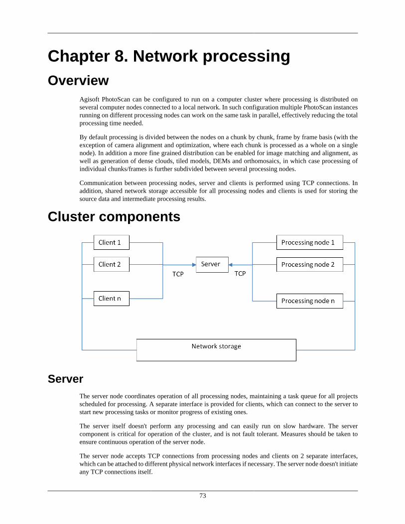
73
Chapter 8. Network processingOverview
Agisoft PhotoScan can be configured to run on a computer cluster where processing is distributed onseveral computer nodes connected to a local network. In such configuration multiple PhotoScan instancesrunning on different processing nodes can work on the same task in parallel, effectively reducing the totalprocessing time needed.
By default processing is divided between the nodes on a chunk by chunk, frame by frame basis (with theexception of camera alignment and optimization, where each chunk is processed as a whole on a singlenode). In addition a more fine grained distribution can be enabled for image matching and alignment, aswell as generation of dense clouds, tiled models, DEMs and orthomosaics, in which case processing ofindividual chunks/frames is further subdivided between several processing nodes.
Communication between processing nodes, server and clients is performed using TCP connections. Inaddition, shared network storage accessible for all processing nodes and clients is used for storing thesource data and intermediate processing results.
Cluster components
ServerThe server node coordinates operation of all processing nodes, maintaining a task queue for all projectsscheduled for processing. A separate interface is provided for clients, which can connect to the server tostart new processing tasks or monitor progress of existing ones.
The server itself doesn't perform any processing and can easily run on slow hardware. The servercomponent is critical for operation of the cluster, and is not fault tolerant. Measures should be taken toensure continuous operation of the server node.
The server node accepts TCP connections from processing nodes and clients on 2 separate interfaces,which can be attached to different physical network interfaces if necessary. The server node doesn't initiateany TCP connections itself.
Network processing
74
Processing nodesProcessing nodes perform actual calculations, and thus need to be run on fast hardware. Each processingnode connects to the server on startup and waits for a task to be assigned. Once the task is available, thenode starts processing, informing the server about the progress. When processing is finished, the resultsare stored on shared network storage, and the server is informed about completion. Then a node switchesto the next task when it becomes available.
Processing nodes can be added or removed from the cluster as needed. Abnormal shutdown of processingnode doesn't cause cluster failure in most cases. Nevertheless, it is highly recommended to stop particularnodes using Agisoft Network Monitor before disconnecting them from the cluster.
ClientsClients can connect to the server node to control cluster operation or to monitor its status. New tasks can besubmitted for processing using Agisoft PhotoScan software configured as a network client, while clustermonitoring is performed using Agisoft Network Monitor. Multiple clients can be connected to the servernode simultaneously.
Cluster setupBefore proceeding to the following steps please make sure that shared network storage is accessible fromall processing and client nodes using the same absolute path. It should be either mounted to the same folderon all nodes (Linux), or should have the same UNC network path (Windows). In case such configurationis not possible (for example in mixed Windows/Linux cluster), a path prefix can be specified on each nodeto compensate for the differences.
Starting serverIt is recommended to configure server with a static IP address, not dynamically assigned one. This IPaddress will be needed for each processing node and client.
The server process can be started by executing PhotoScan with the following command line arguments:photoscan --server --control <ip>[:port] --dispatch <ip>[:port] [--root prefix]
--server parameter specifies that PhotoScan should be started in a server mode.
--control parameter specifies the network interface to be used for communication with clients. In case portvalue is omitted, the default port 5840 is used.
--dispatch parameter specifies the network interface to be used for communication with processing nodes.In case port value is omitted, the default port 5841 is used.
--root parameter can be used to specify network storage mount point or prefix path in case it is not thesame across network.
Example:photoscan --server --control 10.0.1.1 --dispatch 10.0.1.1
In this case PhotoScan will use the same interface for both clients and processing nodes with default portvalues.
Starting network nodesThe processing node can be started by executing PhotoScan with the following command line arguments:
Network processing
75
photoscan --node --dispatch <ip>[:port] [--root prefix]
--node parameter specifies that PhotoScan should be started as a processing node.
--dispatch parameter specifies IP of the server to connect. In case port value is omitted, the default port5841 is used.
--root parameter can be used to specify network storage mount point or prefix path in case it is not thesame across network.
Example:photoscan --node --dispatch 10.0.1.1
This command will start processing node using 10.0.1.1 as a server IP with default port 5841.
Checking cluster statusStart Agisoft Network Monitor application. In the host name field enter server IP used for clientconnections (10.0.1.1 in our example). Modify port values in case non-default port was specified. ClickConnect button when done.
A list of available network nodes currently connected to the server will be displayed in the bottom part ofthe window. Please make sure that all started processing nodes are listed.
The top part lists tasks currently being processed (finished tasks are removed from the list as soon as theyare completed). The task list will be empty if no processing was started yet.
Starting network processing1. Configure Agisoft PhotoScan for network processing.
Start Agisoft PhotoScan on any computer connected to the cluster network.
Open Preferences dialog using Preferences... command from the Tools menu. On the Network tabmake sure Enable network processing option is turned on, and specify the server IP used for clientconnection in the Host name field. In case non-default port was configured on a server, modify theport value accordingly.
In case you are going to process a few single-frame chunks with large number of photos, werecommend to enable fine-level task distribution for all supported operations (Match Photos, AlignCameras, Build Dense Cloud, Build Tiled Model, Build DEM, Build Orthomosaic). In case you aregoing to process a large number of small chunks, or chunks with large number of frames, fine-leveltask distribution can be left in disabled state.
Press OK button when done.
2. Prepare project for network processing.
Open the project file to be processed. Make sure that the project is saved in PhotoScan Project (*.psx)format. Processing of projects in PhotoScan Archive (*.psz) format is not supported in network mode..
Important! Please make sure that source images are located on shared network storage and not on alocal hard drive. Otherwise processing nodes will be unable to load them.
3. Start processing.
Network processing
76
Start processing using corresponding command from the Workflow menu, or using Batch Processcommand to execute a command sequence. A network progress dialog should appear displayingcurrent progress.
4. Wait for processing to complete.
You can disconnect from the server at any time using Disconnect button in the Network Progressdialog in case you need to work on other projects. Processing will continue in the background.
To see processing status after you have disconnected from the server simply open corresponding .psxproject on the network storage. Alternatively you can use Agisoft Network Monitor to see processingstatus for all projects being processed.
5. Inspect processing results.
After processing is finished, click Close button to close Network Progress dialog. The project withprocessing results will be displayed in PhotoScan window.
Cluster administration
Adding processing nodesNew processing nodes can be added by starting Agisoft PhotoScan on additional computers in the networknode mode, as outlined in the Starting network nodes section above.
Removing processing nodesAborting or disconnecting processing node during cluster operation is not absolutely safe, and can lead toproject corruption if performed during final project update at the end of processing. Although the chancesof this situation are relatively low, we strongly recommend against such approach. To safely disconnectprocessing node from the cluster you need to stop processing on this node using Agisoft Network Monitorfirst.
1. Start Agisoft Network Monitor. Make sure the server IP is properly configured in the host name fieldand click Connect button.
2. In the bottom list of network nodes identify the node to be removed. From the node menu selectPause command to stop the node after it finishes current job, or Stop command to abort processingimmediately.
3. Wait until the Batch # and Progress items for a selected node become empty. This indicates that thenode has finished processing. The status of the node should be Paused.
4. Now you can safely disconnect the node by aborting PhotoScan process.

77
Appendix A. Graphical user interfaceApplication window
General view
General view of application window.
Model viewModel view tab is used for displaying 3D data as well as for mesh and point cloud editing. The view ofthe model depends on the current processing stage and is also controlled by mode selection buttons onthe PhotoScan toolbar.
Model can be shown as a dense cloud, with class indication or without, or as a mesh in shaded, solid,wireframe or textured mode. Along with the model the results of photo alignment can be displayed. These
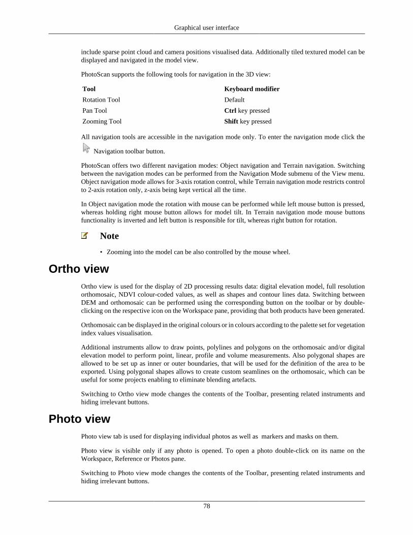
Graphical user interface
78
include sparse point cloud and camera positions visualised data. Additionally tiled textured model can bedisplayed and navigated in the model view.
PhotoScan supports the following tools for navigation in the 3D view:
Tool Keyboard modifier
Rotation Tool Default
Pan Tool Ctrl key pressed
Zooming Tool Shift key pressed
All navigation tools are accessible in the navigation mode only. To enter the navigation mode click the
Navigation toolbar button.
PhotoScan offers two different navigation modes: Object navigation and Terrain navigation. Switchingbetween the navigation modes can be performed from the Navigation Mode submenu of the View menu.Object navigation mode allows for 3-axis rotation control, while Terrain navigation mode restricts controlto 2-axis rotation only, z-axis being kept vertical all the time.
In Object navigation mode the rotation with mouse can be performed while left mouse button is pressed,whereas holding right mouse button allows for model tilt. In Terrain navigation mode mouse buttonsfunctionality is inverted and left button is responsible for tilt, whereas right button for rotation.
Note
• Zooming into the model can be also controlled by the mouse wheel.
Ortho viewOrtho view is used for the display of 2D processing results data: digital elevation model, full resolutionorthomosaic, NDVI colour-coded values, as well as shapes and contour lines data. Switching betweenDEM and orthomosaic can be performed using the corresponding button on the toolbar or by double-clicking on the respective icon on the Workspace pane, providing that both products have been generated.
Orthomosaic can be displayed in the original colours or in colours according to the palette set for vegetationindex values visualisation.
Additional instruments allow to draw points, polylines and polygons on the orthomosaic and/or digitalelevation model to perform point, linear, profile and volume measurements. Also polygonal shapes areallowed to be set up as inner or outer boundaries, that will be used for the definition of the area to beexported. Using polygonal shapes allows to create custom seamlines on the orthomosaic, which can beuseful for some projects enabling to eliminate blending artefacts.
Switching to Ortho view mode changes the contents of the Toolbar, presenting related instruments andhiding irrelevant buttons.
Photo viewPhoto view tab is used for displaying individual photos as well as markers and masks on them.
Photo view is visible only if any photo is opened. To open a photo double-click on its name on theWorkspace, Reference or Photos pane.
Switching to Photo view mode changes the contents of the Toolbar, presenting related instruments andhiding irrelevant buttons.
Graphical user interface
79
Workspace paneOn the Workspace pane all elements comprising the current project are displayed. These elements caninclude:
• List of chunks in the project
• List of cameras and camera groups in each chunk
• List of markers in each chunk
• List of scale bars in each chunk
• Tie points in each chunk
• Depth maps in each chunk
• Dense point clouds in each chunk
• 3D models in each chunk
• Tiled models in each chunk
• Digital elevation models in each chunk
• Orthomosaics in each chunk
• Shapes in each chunk
• Elevation contours in each chunk
Buttons located on the Workspace pane toolbar allow to:
• Add chunk
• Add photos
• Add marker
• Create scale bar
• Enable or disable certain cameras or chunks for processing at further stages.
• Remove items
Each element in the list is linked with the context menu providing quick access to some commonoperations.
Photos panePhotos pane displays the list of photos / masks in the active chunk in the form of thumbnails.
Buttons located on the Photos pane toolbar allow to:
• Enable / disable certain cameras
• Remove cameras
• Rotate selected photos clockwise / counterclockwise
• Reset current photo filtering option
Graphical user interface
80
• Switch between images and masks thumbnails
• Increase / decrease icons' size or display detailed information on photos including EXIF data
Console paneConsole pane is used for:
• Displaying auxiliary information
• Displaying error messages
• Python commands input
Buttons located on the pane toolbar allow:
• Save log
• Clear log
• Execute Python script
Reference paneReference pane is designed for:
• Displaying camera and / or marker coordinates
• Displaying scale bars lengths
• Displaying camera orientations
• Displaying estimation errors
Buttons located on the pane toolbar allow:
• Import / export reference coordinates
• Convert reference coordinates from one system to the other
• Optimize camera alignment and update data
• Switch between source coordinates, estimated coordinates and errors views
• Specify the coordinate system and measurement accuracy to be assumed through Settings dialog
Timeline paneTimeline pane is designed for:
• Working with multi-frame chunks
Buttons located on the pane toolbar allow:
• Add / remove frames from chunk
• Play / stop frame sequence
• Adjust frame rate through Settings dialog
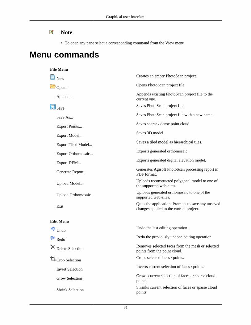
Graphical user interface
81
Note
• To open any pane select a corresponding command from the View menu.
Menu commands
File Menu
NewCreates an empty PhotoScan project.
Open...Opens PhotoScan project file.
Append...Appends existing PhotoScan project file to thecurrent one.
SaveSaves PhotoScan project file.
Save As...Saves PhotoScan project file with a new name.
Export Points...Saves sparse / dense point cloud.
Export Model...Saves 3D model.
Export Tiled Model...Saves a tiled model as hierarchical tiles.
Export Orthomosaic...Exports generated orthomosaic.
Export DEM...Exports generated digital elevation model.
Generate Report...Generates Agisoft PhotoScan processing report inPDF format.
Upload Model...Uploads reconstructed polygonal model to one ofthe supported web-sites.
Upload Orthomosaic...Uploads generated orthomosaic to one of thesupported web-sites.
ExitQuits the application. Prompts to save any unsavedchanges applied to the current project.
Edit Menu
UndoUndo the last editing operation.
RedoRedo the previously undone editing operation.
Delete SelectionRemoves selected faces from the mesh or selectedpoints from the point cloud.
Crop SelectionCrops selected faces / points.
Invert SelectionInverts current selection of faces / points.
Grow SelectionGrows current selection of faces or sparse cloudpoints.
Shrink SelectionShrinks current selection of faces or sparse cloudpoints.
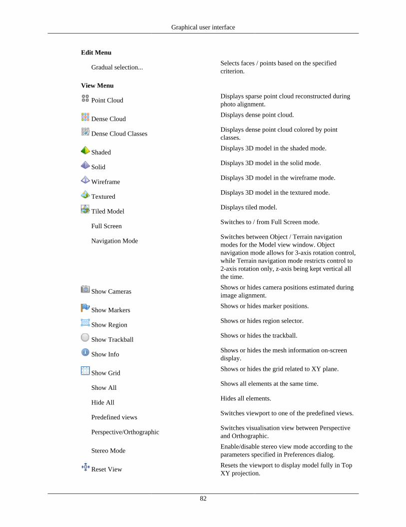
Graphical user interface
82
Edit Menu
Gradual selection...Selects faces / points based on the specifiedcriterion.
View Menu
Point CloudDisplays sparse point cloud reconstructed duringphoto alignment.
Dense CloudDisplays dense point cloud.
Dense Cloud ClassesDisplays dense point cloud colored by pointclasses.
ShadedDisplays 3D model in the shaded mode.
SolidDisplays 3D model in the solid mode.
WireframeDisplays 3D model in the wireframe mode.
TexturedDisplays 3D model in the textured mode.
Tiled ModelDisplays tiled model.
Full ScreenSwitches to / from Full Screen mode.
Navigation ModeSwitches between Object / Terrain navigationmodes for the Model view window. Objectnavigation mode allows for 3-axis rotation control,while Terrain navigation mode restricts control to2-axis rotation only, z-axis being kept vertical allthe time.
Show CamerasShows or hides camera positions estimated duringimage alignment.
Show MarkersShows or hides marker positions.
Show RegionShows or hides region selector.
Show TrackballShows or hides the trackball.
Show InfoShows or hides the mesh information on-screendisplay.
Show GridShows or hides the grid related to XY plane.
Show AllShows all elements at the same time.
Hide AllHides all elements.
Predefined viewsSwitches viewport to one of the predefined views.
Perspective/OrthographicSwitches visualisation view between Perspectiveand Orthographic.
Stereo ModeEnable/disable stereo view mode according to theparameters specified in Preferences dialog.
Reset ViewResets the viewport to display model fully in TopXY projection.

Graphical user interface
83
View Menu
WorkspaceShows or hides Workspace pane.
TimelineShows or hides Timeline pane.
ReferenceShows or hides Reference pane.
PhotosShows or hides Photos pane.
ConsoleShows or hides Console pane.
ToolbarShows or hides Toolbar.
Workflow Menu
Add Photos...Loads additional photos to be processed byPhotoScan.
Add Folder...Loads additional photos from folders to beprocessed by PhotoScan.
Align Photos...Generates camera positions and sparse point cloud.
Build Dense Cloud...Generates dense point cloud.
Build Mesh...Generates polygonal model.
Build Texture...Generates 3D model texture.
Build Tiled Model...Generates tiled textured model from the densecloud.
Build DEM...Generates digital elevation model.
Build Orthomosaic...Generates orthomosaic.
Align Chunks...Aligns multiple chunks.
Merge Chunks...Merges multiple chunks into the single chunk.
Batch Process...Opens Batch Process dialog box.
Tools Menu
Detect Markers...Creates markers from coded targets on photos.
Track Markers...Tracks marker locations across the framesequence.
Print Markers...Generates printable PDF file with coded targets.
Build Point Cloud...Builds sparse point cloud based on the estimatedcamera parameters available.
Thin Point Cloud...Thins sparse point cloud by reducing the numberof projections on the individual photos to the givenlimit.
Classify Ground Points...Classifies dense point cloud based on the userdefined settings.
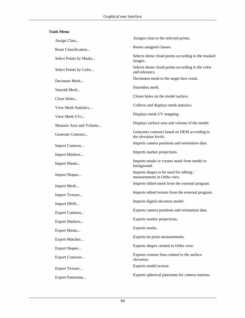
Graphical user interface
84
Tools Menu
Assign Class...Assigns class to the selected points.
Reset Classification...Resets assigned classes.
Select Points by Masks...Selects dense cloud points according to the maskedimages.
Select Points by Color...Selects dense cloud points according to the colorand tolerance.
Decimate Mesh...Decimates mesh to the target face count.
Smooth Mesh...Smoothes mesh.
Close Holes...Closes holes on the model surface.
View Mesh Statistics...Collects and displays mesh statistics.
View Mesh UVs...Displays mesh UV mapping.
Measure Area and Volume...Displays surface area and volume of the model.
Generate Contours...Generates contours based on DEM according tothe elevation levels.
Import Cameras...Imports camera positions and orientation data.
Import Markers...Imports marker projections.
Import Masks...Imports masks or creates mask from model orbackground.
Import Shapes...Imports shapes to be used for editing /measurements in Ortho view.
Import Mesh...Imports edited mesh from the external program.
Import Texture...Imports edited texture from the external program.
Import DEM...Imports digital elevation model.
Export Cameras...Exports camera positions and orientation data.
Export Markers...Exports marker projections.
Export Masks...Exports masks.
Export Matches...Exports tie point measurements.
Export Shapes...Exports shapes created in Ortho view.
Export Contours...Exports contour lines related to the surfaceelevation.
Export Texture...Exports model texture.
Export Panorama...Exports spherical panorama for camera stations.
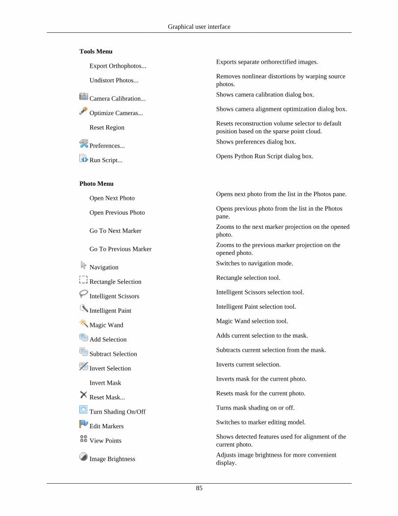
Graphical user interface
85
Tools Menu
Export Orthophotos...Exports separate orthorectified images.
Undistort Photos...Removes nonlinear distortions by warping sourcephotos.
Camera Calibration...Shows camera calibration dialog box.
Optimize Cameras...Shows camera alignment optimization dialog box.
Reset RegionResets reconstruction volume selector to defaultposition based on the sparse point cloud.
Preferences...Shows preferences dialog box.
Run Script...Opens Python Run Script dialog box.
Photo Menu
Open Next PhotoOpens next photo from the list in the Photos pane.
Open Previous PhotoOpens previous photo from the list in the Photospane.
Go To Next MarkerZooms to the next marker projection on the openedphoto.
Go To Previous MarkerZooms to the previous marker projection on theopened photo.
NavigationSwitches to navigation mode.
Rectangle SelectionRectangle selection tool.
Intelligent ScissorsIntelligent Scissors selection tool.
Intelligent PaintIntelligent Paint selection tool.
Magic WandMagic Wand selection tool.
Add SelectionAdds current selection to the mask.
Subtract SelectionSubtracts current selection from the mask.
Invert SelectionInverts current selection.
Invert MaskInverts mask for the current photo.
Reset Mask...Resets mask for the current photo.
Turn Shading On/OffTurns mask shading on or off.
Edit MarkersSwitches to marker editing model.
View PointsShows detected features used for alignment of thecurrent photo.
Image BrightnessAdjusts image brightness for more convenientdisplay.

Graphical user interface
86
Help Menu
ContentsDisplays help contents.
Check for Updates...Checks if PhotoScan update is available fordownload.
Activate Product...Activates / deactivates the product using theactivation key.
About PhotoScan...Displays program information, version number andcopyright.
Toolbar buttons
General commands
NewCreates a new PhotoScan project file.
OpenOpens a PhotoScan project file.
SaveSaves a PhotoScan project file.
3D view commands
UndoUndo the last editing operation.
RedoRedo the previously undone editing operation.
NavigationNavigation tool.
Rectangle SelectionRectangle selection tool.
Circle SelectionCircle selection tool.
Free-Form SelectionFree-form selection tool.
Resize regionVolume selection tool.
Rotate RegionVolume rotation tool.
Rotate ObjectModel rotation tool.
Delete SelectionRemoves selected faces / points.
Crop SelectionCrops selected faces / points.
3D view settings
Point CloudDisplays sparse point cloud reconstructed duringimage alignment.
Dense CloudDisplays dense point cloud model.
Dense Cloud ClassesDisplays dense point cloud coloured by pointclasses.
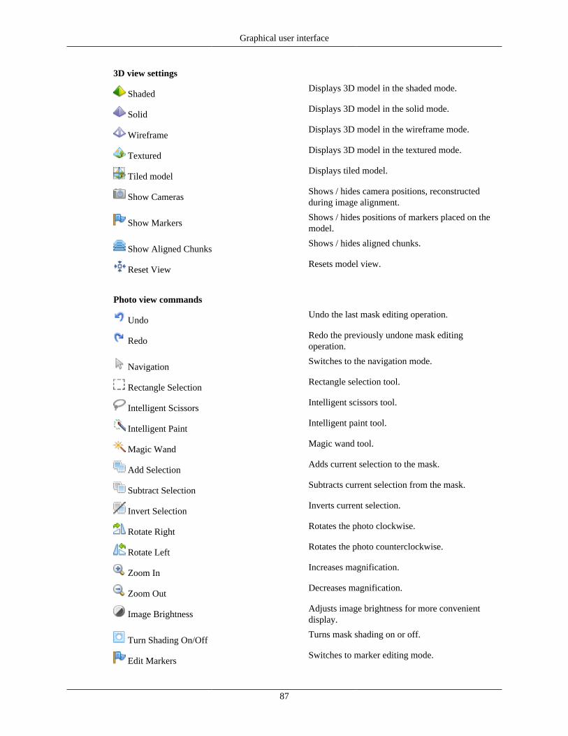
Graphical user interface
87
3D view settings
ShadedDisplays 3D model in the shaded mode.
SolidDisplays 3D model in the solid mode.
WireframeDisplays 3D model in the wireframe mode.
TexturedDisplays 3D model in the textured mode.
Tiled modelDisplays tiled model.
Show CamerasShows / hides camera positions, reconstructedduring image alignment.
Show MarkersShows / hides positions of markers placed on themodel.
Show Aligned ChunksShows / hides aligned chunks.
Reset ViewResets model view.
Photo view commands
UndoUndo the last mask editing operation.
RedoRedo the previously undone mask editingoperation.
NavigationSwitches to the navigation mode.
Rectangle SelectionRectangle selection tool.
Intelligent ScissorsIntelligent scissors tool.
Intelligent PaintIntelligent paint tool.
Magic WandMagic wand tool.
Add SelectionAdds current selection to the mask.
Subtract SelectionSubtracts current selection from the mask.
Invert SelectionInverts current selection.
Rotate RightRotates the photo clockwise.
Rotate LeftRotates the photo counterclockwise.
Zoom InIncreases magnification.
Zoom OutDecreases magnification.
Image BrightnessAdjusts image brightness for more convenientdisplay.
Turn Shading On/OffTurns mask shading on or off.
Edit MarkersSwitches to marker editing mode.
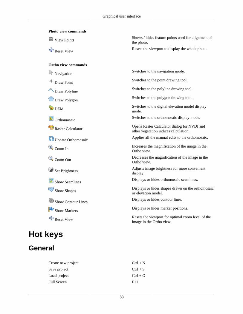
Graphical user interface
88
Photo view commands
View PointsShows / hides feature points used for alignment ofthe photo.
Reset ViewResets the viewport to display the whole photo.
Ortho view commands
NavigationSwitches to the navigation mode.
Draw PointSwitches to the point drawing tool.
Draw PolylineSwitches to the polyline drawing tool.
Draw PolygonSwitches to the polygon drawing tool.
DEMSwitches to the digital elevation model displaymode.
OrthomosaicSwitches to the orthomosaic display mode.
Raster CalculatorOpens Raster Calculator dialog for NVDI andother vegetation indices calculation.
Update OrthomosaicApplies all the manual edits to the orthomosaic.
Zoom InIncreases the magnification of the image in theOrtho view.
Zoom OutDecreases the magnification of the image in theOrtho view.
Set BrightnessAdjusts image brightness for more convenientdisplay.
Show SeamlinesDisplays or hides orthomosaic seamlines.
Show ShapesDisplays or hides shapes drawn on the orthomosaicor elevation model.
Show Contour LinesDisplays or hides contour lines.
Show MarkersDisplays or hides marker positions.
Reset ViewResets the viewport for optimal zoom level of theimage in the Ortho view.
Hot keys
General
Create new project Ctrl + N
Save project Ctrl + S
Load project Ctrl + O
Full Screen F11

Graphical user interface
89
Model ViewUndo (only for Delete, Assign Class / ClassifyGround Points,Masking and Close Holesoperations)
Ctrl + Z
Redo (only for Delete, Assign Class / ClassifyGround Points,Masking and Close Holesoperations)
Ctrl + Y
Switch between navigation and any otherpreviously selected mode
Space
Reset view 0
Switch to stereoview mode 9
Switch between orthographic and perspective viewmodes
5
Change the angle for perspective view Ctrl + mouse wheel
Assign dense cloud class (only if some points areselected)
Ctrl + Shift + C
Predefined Views
Top 7
Bottom Ctrl + 7
Right 3
Left Ctrl + 3
Front 1
Back Ctrl + 1
Rotate View
Rotate Up 8
Rotate Down 2
Rotate Left 4
Rotate Right 6
Photo ViewNext photo (according to Photos pane order) Page Up
Previous photo (according to Photos pane order) Page Down
Go to the next marker on the same photo Tab
Go to the previous marker on the same photo Shift + Tab
Navigation mode V
Selection Tools
Rectangle selection M
Intelligent scissors L
Intelligent paint P
Magic wand W
Add selection Ctrl + Shift + A

Graphical user interface
90
Selection Tools
Subtract selection Ctrl + Shift + S
Invert selection Ctrl + Shift + I
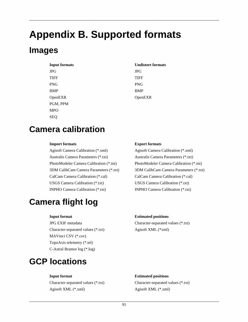
91
Appendix B. Supported formats
Images
Input formats Undistort formats
JPG JPG
TIFF TIFF
PNG PNG
BMP BMP
OpenEXR OpenEXR
PGM, PPM
MPO
SEQ
Camera calibration
Import formats Export formats
Agisoft Camera Calibration (*.xml) Agisoft Camera Calibration (*.xml)
Australis Camera Parameters (*.txt) Australis Camera Parameters (*.txt)
PhotoModeler Camera Calibration (*.ini) PhotoModeler Camera Calibration (*.ini)
3DM CalibCam Camera Parameters (*.txt) 3DM CalibCam Camera Parameters (*.txt)
CalCam Camera Calibration (*.cal) CalCam Camera Calibration (*.cal)
USGS Camera Calibration (*.txt) USGS Camera Calibration (*.txt)
INPHO Camera Calibration (*.txt) INPHO Camera Calibration (*.txt)
Camera flight log
Input format Estimated positions
JPG EXIF metadata Character-separated values (*.txt)
Character-separated values (*.txt) Agisoft XML (*xml)
MAVinci CSV (*.csv)
TopoAxis telemetry (*.tel)
C-Astral Bramor log (*.log)
GCP locations
Input format Estimated positions
Character-separated values (*.txt) Character-separated values (*.txt)
Agisoft XML (*.xml) Agisoft XML (*.xml)
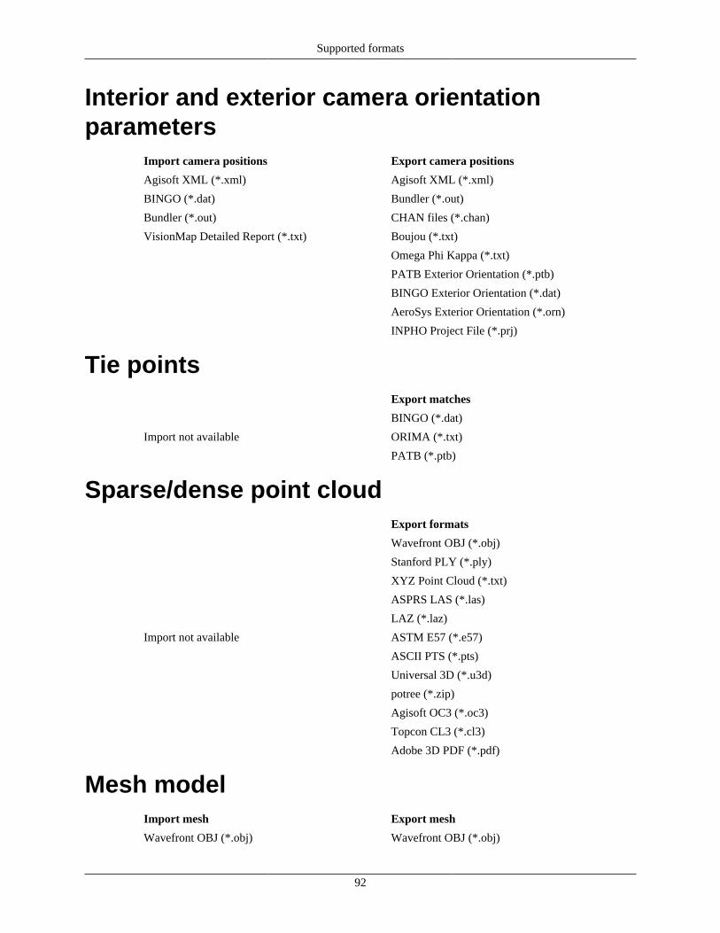
Supported formats
92
Interior and exterior camera orientationparameters
Import camera positions Export camera positions
Agisoft XML (*.xml) Agisoft XML (*.xml)
BINGO (*.dat) Bundler (*.out)
Bundler (*.out) CHAN files (*.chan)
VisionMap Detailed Report (*.txt) Boujou (*.txt)
Omega Phi Kappa (*.txt)
PATB Exterior Orientation (*.ptb)
BINGO Exterior Orientation (*.dat)
AeroSys Exterior Orientation (*.orn)
INPHO Project File (*.prj)
Tie points Export matches
BINGO (*.dat)
Import not available ORIMA (*.txt)
PATB (*.ptb)
Sparse/dense point cloud Export formats
Wavefront OBJ (*.obj)
Stanford PLY (*.ply)
XYZ Point Cloud (*.txt)
ASPRS LAS (*.las)
LAZ (*.laz)
Import not available ASTM E57 (*.e57)
ASCII PTS (*.pts)
Universal 3D (*.u3d)
potree (*.zip)
Agisoft OC3 (*.oc3)
Topcon CL3 (*.cl3)
Adobe 3D PDF (*.pdf)
Mesh modelImport mesh Export mesh
Wavefront OBJ (*.obj) Wavefront OBJ (*.obj)

Supported formats
93
Import mesh Export mesh
3DS models (*.3ds) 3DS models (*.3ds)
COLLADA (*.dae) COLLADA (*.dae)
Stanford PLY (*.ply) Stanford PLY (*.ply)
STL models (*.stl) STL models (*.stl)
Autodesk DXF (*.dxf) Autodesk DXF (*.dxf)
Autodesk FBX (*.fbx) Autodesk FBX (*.fbx)
Universal 3D models (*.u3d) Universal 3D models (*.u3d)
OpenCTM models VRML models (*.wrl)
Adobe 3D PDF (*.pdf)
Texture
Import texture Export texture
JPG JPG
TIFF TIFF
PNG PNG
BMP BMP
OpenEXR OpenEXR
PGM, PPM PGM, PPM
Orthomosaic
Export orthomosaic
GeoTIFF
JPG
PNG
Import not available Google Earth KML/KMZ
Google Map Tiles
MBTiles
World Wind Tiles
Digital elevation model (DSM/DTM)
Import DEM Export DEM
GeoTIFF elevation (*.tif) GeoTIFF elevation (*.tif)
Arc/Info ASCII Grid (*.asc)
Band interleaved file format (*.bil)
XYZ (*.xyz)
Sputnik KMZ (*.kmz)
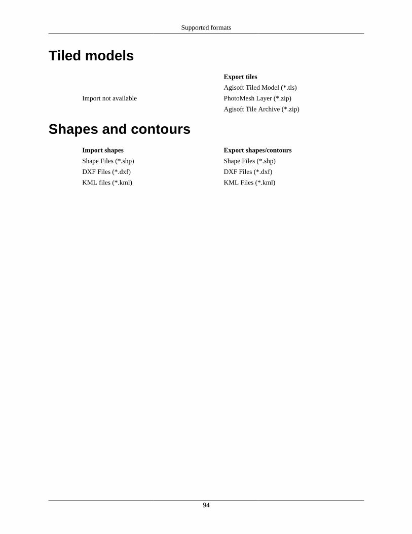
Supported formats
94
Tiled models Export tiles
Agisoft Tiled Model (*.tls)
Import not available PhotoMesh Layer (*.zip)
Agisoft Tile Archive (*.zip)
Shapes and contoursImport shapes Export shapes/contours
Shape Files (*.shp) Shape Files (*.shp)
DXF Files (*.dxf) DXF Files (*.dxf)
KML files (*.kml) KML Files (*.kml)
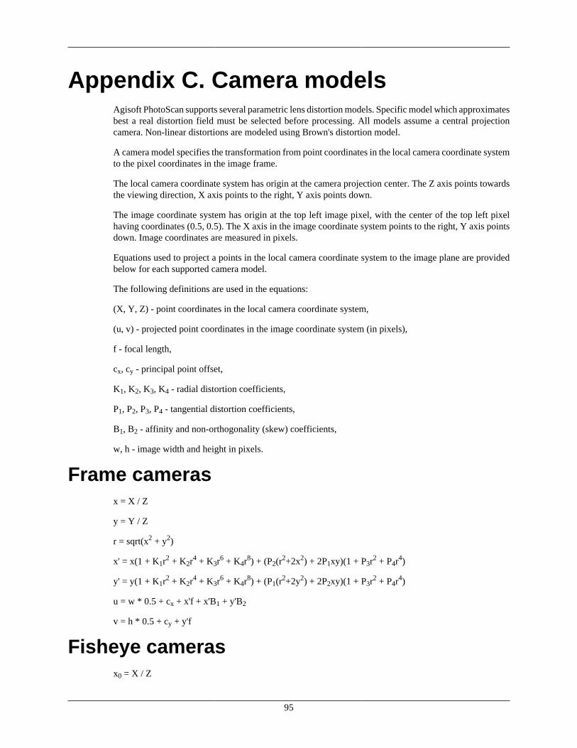
95
Appendix C. Camera modelsAgisoft PhotoScan supports several parametric lens distortion models. Specific model which approximatesbest a real distortion field must be selected before processing. All models assume a central projectioncamera. Non-linear distortions are modeled using Brown's distortion model.
A camera model specifies the transformation from point coordinates in the local camera coordinate systemto the pixel coordinates in the image frame.
The local camera coordinate system has origin at the camera projection center. The Z axis points towardsthe viewing direction, X axis points to the right, Y axis points down.
The image coordinate system has origin at the top left image pixel, with the center of the top left pixelhaving coordinates (0.5, 0.5). The X axis in the image coordinate system points to the right, Y axis pointsdown. Image coordinates are measured in pixels.
Equations used to project a points in the local camera coordinate system to the image plane are providedbelow for each supported camera model.
The following definitions are used in the equations:
(X, Y, Z) - point coordinates in the local camera coordinate system,
(u, v) - projected point coordinates in the image coordinate system (in pixels),
f - focal length,
cx, cy - principal point offset,
K1, K2, K3, K4 - radial distortion coefficients,
P1, P2, P3, P4 - tangential distortion coefficients,
B1, B2 - affinity and non-orthogonality (skew) coefficients,
w, h - image width and height in pixels.
Frame camerasx = X / Z
y = Y / Z
r = sqrt(x2 + y2)
x' = x(1 + K1r2 + K2r4 + K3r6 + K4r8) + (P2(r2+2x2) + 2P1xy)(1 + P3r2 + P4r4)
y' = y(1 + K1r2 + K2r4 + K3r6 + K4r8) + (P1(r2+2y2) + 2P2xy)(1 + P3r2 + P4r4)
u = w * 0.5 + cx + x'f + x'B1 + y'B2
v = h * 0.5 + cy + y'f
Fisheye camerasx0 = X / Z

Camera models
96
y0 = Y / Z
r0 = sqrt(x02 + y0
2)
x = x0 * tan-1r0 / r0
y = y0 * tan-1r0 / r0
r = sqrt(x2 + y2)
x' = x(1 + K1r2 + K2r4 + K3r6 + K4r8) + (P2(r2+2x2) + 2P1xy)(1 + P3r2 + P4r4)
y' = y(1 + K1r2 + K2r4 + K3r6 + K4r8) + (P1(r2+2y2) + 2P2xy)(1 + P3r2 + P4r4)
u = w * 0.5 + cx + x'f + x'B1 + y'B2
v = h * 0.5 + cy + y'f
Spherical cameras (equirectangular projection)u = w * 0.5 + f * tan-1(X / Z)
v = h * 0.5 + f * tan-1(Y / sqrt(X2 + Z2))
where:
f = w / (2 * pi)
Note
• Spherical (equirectangular) camera model doesn't support distortions. All distortions should becorrected before loading images in PhotoScan.
• In case you are capturing panoramas with a rotated frame/fisheye camera, we recommend toprocess original images in PhotoScan using camera station function instead of stitching them inexternal software.
Spherical cameras (cylindrical projection)u = w * 0.5 + f * tan-1(X / Z)
v = h * 0.5 + f * Y / sqrt(X2 + Z2)
where:
f = w / (2 * pi)
Note
• Spherical (cylindrical) camera model doesn't support distortions. All distortions should becorrected before loading images in PhotoScan.
• In case you are capturing panoramas with a rotated frame/fisheye camera, we recommend toprocess original images in PhotoScan using camera station function instead of stitching them inexternal software.