Robotics 1

Inverse kinematicsProf. Alessandro De Luca

Robotics 1 1

Inverse kinematicswhat are we looking for?

Robotics 1 2

direct kinematics is always unique;how about inverse kinematics for this 6R robot?

�

Inverse kinematics problem

n “given a desired end-effector pose (position + orientation), find the values of the joint variables that will realize it”

n a synthesis problem, with input data in the form

n T = = 0An(q)

n a typical nonlinear problemn existence of a solution (workspace definition)n uniqueness/multiplicity of solutions (r Î Rm, q ÎRn)n solution methods

R p000 1

pf

§ r = = fr(q), or for any other task vector

Robotics 1 3

classical formulation:inverse kinematics for a given end-effector pose

generalized formulation:inverse kinematics for a given value of task variables

Solvability and robot workspace(for tasks related to a desired end-effector Cartesian pose)

n primary workspace WS1: set of all positions p that can be reached with at least one orientation (f or R)n out of WS1 there is no solution to the problemn when p Î WS1, there is a suitable f (or R) for which a solution exists

n secondary (or dexterous) workspace WS2: set of positions p that can be reached with any orientation (among those feasible for the robot direct kinematics)n when p Î WS2, there exists a solution for any feasible f (or R)

n WS2 Í WS1

Robotics 1 4

Workspace of Fanuc R-2000i/165F

WS1⊂R3(≈ WS2 for spherical wrist

without joint limits)

Robotics 1 5

section for aconstant angle q1

rotating the base joint angle q1

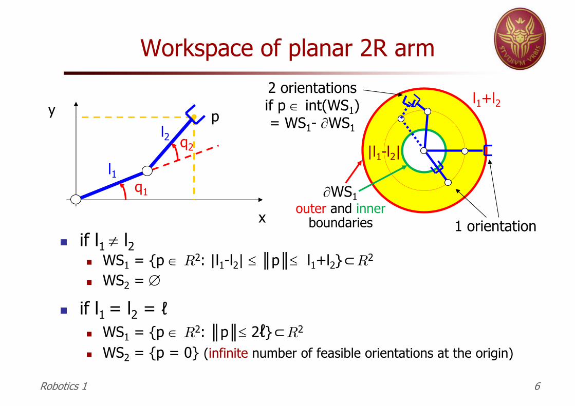
Workspace of planar 2R arm

n if l1 ¹ l2n WS1 = {p Î R2: |l1-l2| £ ║p║£ l1+l2}⊂R2

n WS2 = Æ

n if l1 = l2 = ℓn WS1 = {p Î R2: ║p║£ 2ℓ}⊂R2

n WS2 = {p = 0} (infinite number of feasible orientations at the origin)

x

y • p

l1

l2

q1

q2

l1+l2

|l1-l2|

2 orientationsif p Î int(WS1)= WS1- ¶WS1

1 orientation

¶WS1

Robotics 1 6

outer and innerboundaries

Wrist position and E-E poseinverse solutions for an articulated 6R robot

LEFT DOWN RIGHT DOWN

LEFT UP RIGHT UP

4 inverse solutionsout of singularities(for the position of

the wrist center only)

8 inverse solutions consideringthe complete E-E pose

(spherical wrist: 2 alternative solutions for the last 3 joints)

Unimation PUMA 560

Robotics 1 7

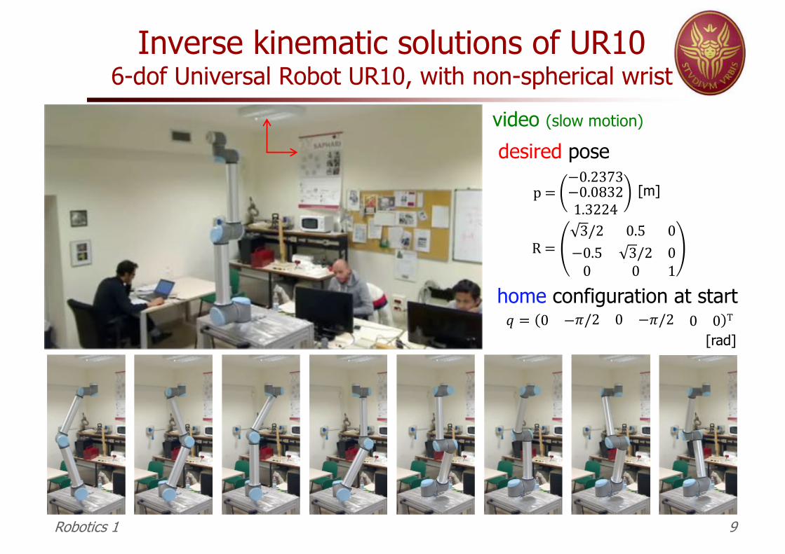
Inverse kinematic solutions of UR106-dof Universal Robot UR10, with non-spherical wrist

Robotics 1 9

video (slow motion)

desired pose

home configuration at start

[rad]

[m]p=−0.2373−0.08321.3224

R =3/2 0.5 0−0.5 3/2 00 0 1

0 = 0 −1/2 0 −1/2 0 0 T

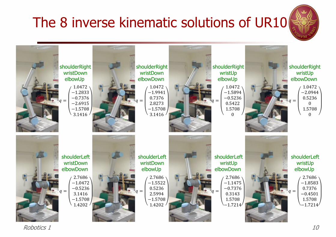
The 8 inverse kinematic solutions of UR10

Robotics 1 10

shoulderRightwristDownelbowUp

shoulderRightwristDown

elbowDown

shoulderRightwristUp

elbowUp

shoulderRightwristUp

elbowDown

shoulderLeftwristDown

elbowDown

shoulderLeftwristDownelbowUp

shoulderLeftwristUp

elbowDown

shoulderLeftwristUp

elbowUp

! =

1.0472−1.2833−0.7376−2.6915−1.57083.1416

! =

1.0472−1.99410.73762.8273−1.57083.1416

! =

1.0472−1.5894−0.52360.54221.57080

! =

1.0472−2.09440.52360

1.57080

! =

2.7686−1.85830.7376−0.45011.5708−1.7214

! =

2.7686−1.1475−0.73760.31431.5708−1.7214

! =

2.7686−1.55220.52362.5994−1.57081.4202

! =

2.7686−1.0472−0.52363.1416−1.57081.4202

Multiplicity of solutionssome examples

n E-E positioning (m=2) of a planar 2R robot arm

n 2 regular solutions in int(WS1)

n 1 solution on ¶WS1

n for l1 = l2: ¥ solutions in WS2

n E-E positioning of an articulated elbow-type 3R robot arm

n 4 regular solutions in WS1 (with singular cases yet to be investigated ...)

n spatial 6R robot arms

n £ 16 distinct solutions, out of singularities: this “upper bound” of

solutions was shown to be attained by a particular instance of

“orthogonal” robot, i.e., with twist angles ai = 0 or ±p/2 ("i)

n analysis based on algebraic transformations of robot kinematics

n transcendental equations are transformed into a single polynomial

equation of one variable

n seek for an equivalent polynomial equation of the least possible degree

singular solutions

Robotics 1 11

1. in WS1 : ¥1 regular solutions (except for 2. and 3.), at which the E-E can take a continuum of ¥ orientations (but not all orientations in the plane!)

2. if ║p║= 3ℓ : only 1 solution, singular

3. if ║p║= ℓ : ¥1 solutions, 3 of which singular

4. if ║p║< ℓ : ¥1 regular solutions (never singular)

A planar 3R armworkspace and number/type of inverse solutions

x

y• p

l1

l2

q1

q2

l3

q3 l1 = l2 = l3 = ℓ, n=3, m=2

WS1 = {p Î R2: ║p║£ 3ℓ}⊂R2

WS2 = {p Î R2: ║p║£ ℓ}⊂R2

any planar orientation is feasible in WS2

Robotics 1 12

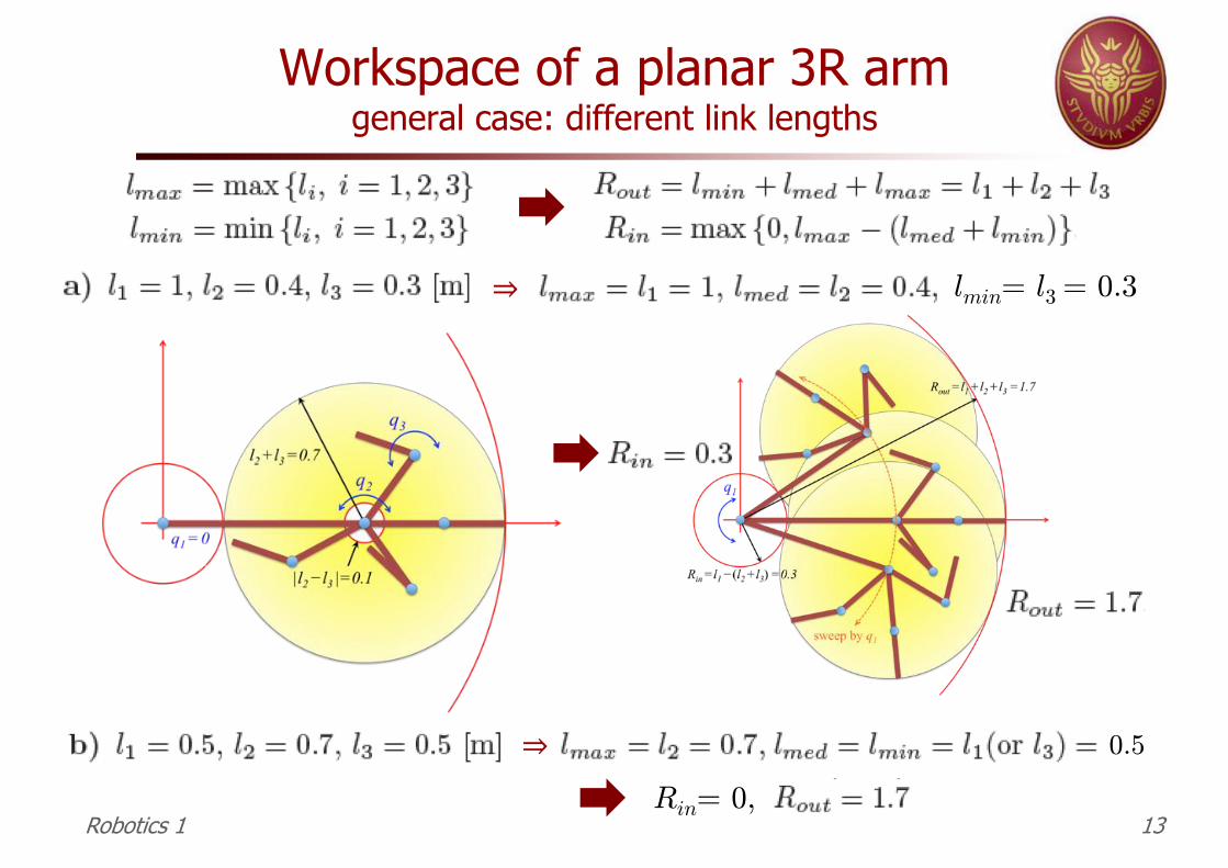
Workspace of a planar 3R armgeneral case: different link lengths

Robotics 1 13

lmin= l3 = 0.3⇒

⇒Rin= 0,

0.5

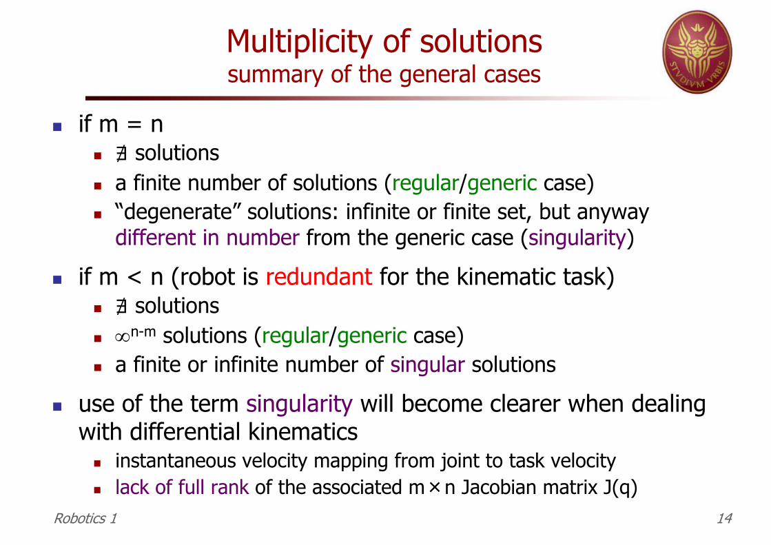
Multiplicity of solutionssummary of the general cases

n if m = nn ∄ solutionsn a finite number of solutions (regular/generic case)n “degenerate” solutions: infinite or finite set, but anyway

different in number from the generic case (singularity)

n if m < n (robot is redundant for the kinematic task)n ∄ solutionsn ¥n-m solutions (regular/generic case)n a finite or infinite number of singular solutions

n use of the term singularity will become clearer when dealing with differential kinematics

n instantaneous velocity mapping from joint to task velocityn lack of full rank of the associated m�n Jacobian matrix J(q)

Robotics 1 14

Dexter robot (8R arm)n m = 6 (position and orientation of E-E)n n = 8 (all revolute joints)n ¥2 inverse kinematic solutions (redundancy degree = n-m = 2)

exploring inverse kinematic solutions by a self-motion

video

Robotics 1 15

Solution methods

ANALYTICAL solution(in closed form)

NUMERICAL solution(in iterative form)

§ preferred, if it can be found*§ use ad-hoc geometric inspection§ algebraic methods (solution of

polynomial equations)§ systematic ways for generating a

reduced set of equations to be solved

* sufficient conditions for 6-dof arms• 3 consecutive rotational joint axes are

incident (e.g., spherical wrist), or• 3 consecutive rotational joint axes are

parallel

§ certainly needed if n>m (redundant case), or at/close to singularities

§ slower, but easier to be set up§ in its basic form, it uses the

(analytical) Jacobian matrix of the direct kinematics map

§ Newton method, Gradient method, and so on…

Jr(q) = ¶fr (q)¶q

Robotics 1 16D. Pieper, PhD thesis, Stanford University, 1968

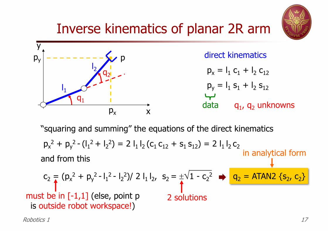
Inverse kinematics of planar 2R arm

x

y• p

l1

l2

q1

q2

px

py direct kinematicspx = l1 c1 + l2 c12

py = l1 s1 + l2 s12

data q1, q2 unknowns

“squaring and summing” the equations of the direct kinematicspx

2 + py2 - (l12 + l22) = 2 l1 l2 (c1 c12 + s1 s12) = 2 l1 l2 c2

and from this

c2 = (px2 + py

2 - l12 - l22)/ 2 l1 l2, s2 = ±Ö1 - c22 q2 = ATAN2 {s2, c2}

2 solutions

in analytical form

must be in [-1,1] (else, point pis outside robot workspace!)

Robotics 1 17

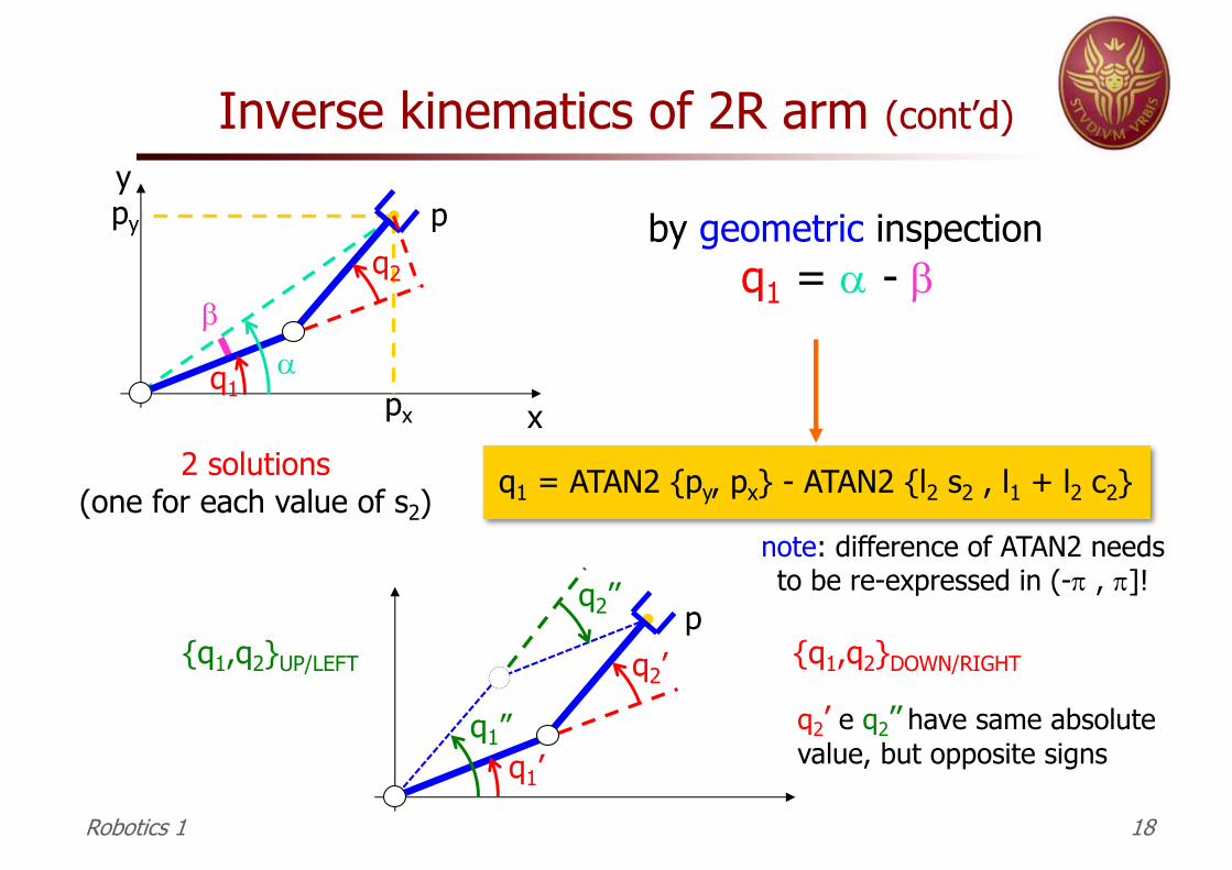
Inverse kinematics of 2R arm (cont’d)

x

y• p

q1

q2

px

py

q1 = ATAN2 {py, px} - ATAN2 {l2 s2 , l1 + l2 c2}

a

b

by geometric inspectionq1 = a - b

2 solutions (one for each value of s2)

note: difference of ATAN2 needsto be re-expressed in (-p , p]!

q2’ e q2’’ have same absolute value, but opposite signs

Robotics 1 18

• p

q1’

q2’

q2’’

q1”

{q1,q2}UP/LEFT {q1,q2}DOWN/RIGHT

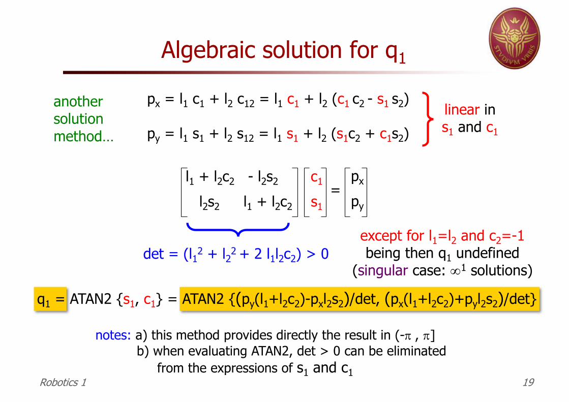
Algebraic solution for q1

l1 + l2c2 - l2s2

l2s2 l1 + l2c2

c1

s1

px

py=

q1 = ATAN2 {s1, c1} = ATAN2 {(py(l1+l2c2)-pxl2s2)/det, (px(l1+l2c2)+pyl2s2)/det}

det = (l12 + l22 + 2 l1l2c2) > 0except for l1=l2 and c2=-1being then q1 undefined

(singular case: ¥1 solutions)

notes: a) this method provides directly the result in (-p , p]b) when evaluating ATAN2, det > 0 can be eliminated

from the expressions of s1 and c1

px = l1 c1 + l2 c12 = l1 c1 + l2 (c1 c2 - s1 s2)

py = l1 s1 + l2 s12 = l1 s1 + l2 (s1c2 + c1s2)

linear ins1 and c1

another solution method…

Robotics 1 19

Robotics 1 20

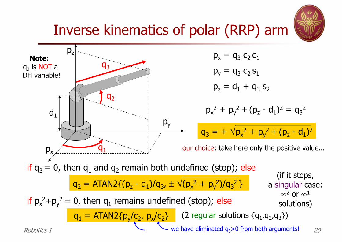
Inverse kinematics of polar (RRP) arm

px

py

pz

q1

q2

q3

d1

px = q3 c2 c1

py = q3 c2 s1

pz = d1 + q3 s2

q1 = ATAN2{py/c2, px/c2}

if px2+py

2 = 0, then q1 remains undefined (stop); else (2 regular solutions {q1,q2,q3})

q2 = ATAN2{(pz - d1)/q3, ± Ö(px2 + py

2)/q32 }

if q3 = 0, then q1 and q2 remain both undefined (stop); else (if it stops,

a singular case: ¥2 or ¥1

solutions)

we have eliminated q3>0 from both arguments!

px2 + py

2 + (pz - d1)2 = q32

q3 = + Öpx2 + py

2 + (pz - d1)2

our choice: take here only the positive value...

Note:q2 is NOT aDH variable!

Robotics 1 21

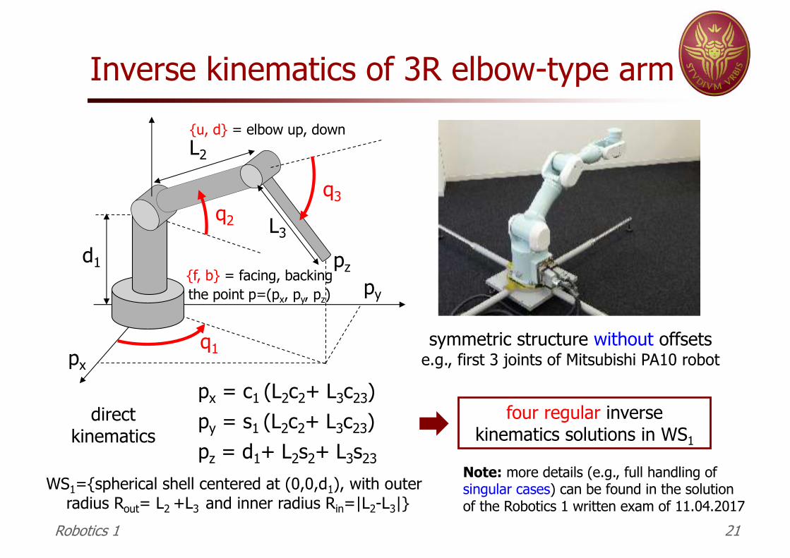
Inverse kinematics of 3R elbow-type arm

px

py

pz

q1

q2

q3

d1

L2

L3

symmetric structure without offsetse.g., first 3 joints of Mitsubishi PA10 robot

px = c1 (L2c2+ L3c23)py = s1 (L2c2+ L3c23)pz = d1+ L2s2+ L3s23

directkinematics

Note: more details (e.g., full handling of singular cases) can be found in the solution of the Robotics 1 written exam of 11.04.2017

{f, b} = facing, backingthe point p=(px, py, pz)

{u, d} = elbow up, down

four regular inverse kinematics solutions in WS1

WS1={spherical shell centered at (0,0,d1), with outer radius Rout= L2 +L3 and inner radius Rin=|L2-L3|}

Robotics 1 22

Inverse kinematics of 3R elbow-type arm

px

py

pz

q1

q2

q3

d1

L2

L3

px2 + py

2 + (pz-d1)2 = c12 (L2c2+ L3c23)2 + s1

2 (L2c2+ L3c23)2 + (L2s2+ L3s23)2

= ... = L22 + L3

2 + 2L2L3 (c2c23+s2s23) = L22 + L3

2 + 2L2L3 c3

c3 = (px2 + py

2 + (pz-d1)2 - L22 - L3

2) / 2L2L3 ∈ [-1,1] (else, p is out of workspace!)

q3{+} = ATAN2{s3, c3}

q3{-} = ATAN2{-s3, c3} = - q3

{+}two solutions�s3 = �Ö1 - c3

2

px = c1 (L2c2+ L3c23)py = s1 (L2c2+ L3c23)pz = d1+ L2s2+ L3s23

directkinematics

Robotics 1 23

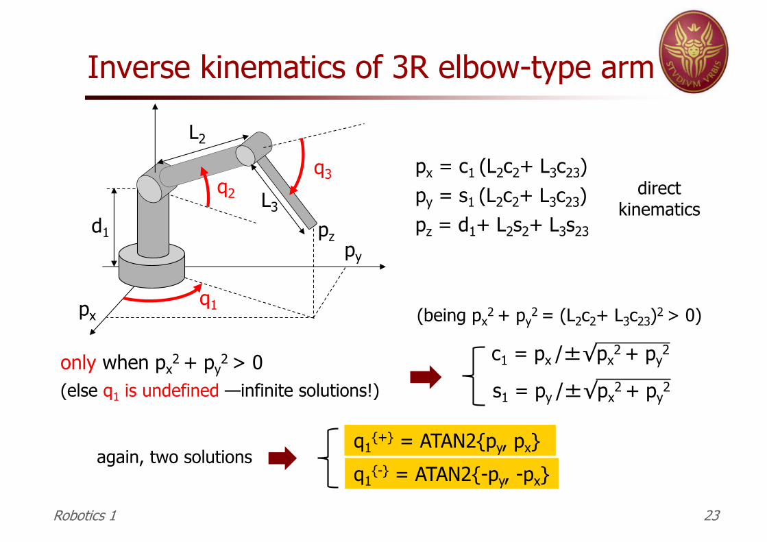
Inverse kinematics of 3R elbow-type arm

only when px2 + py

2 > 0

(else q1

is undefined —infinite solutions!)

px

py

pz

q1

q2

q3

d1

L2

L3

(being px2 + p

y2 = (L

2c

2+ L

3c

23)2 > 0)

q1{+} = ATAN2{py, px}

q1{-} = ATAN2{-p

y, -p

x}

again, two solutions

c1 = px /�√px2 + py

2

s1 = py /�√px2 + py

2

px = c1 (L2c2+ L3c23)

py

= s1 (L

2c

2+ L

3c

23)

pz = d1+ L2s2+ L3s23

direct

kinematics

Robotics 1 24

Inverse kinematics of 3R elbow-type arm

px

py

pz

q1

q2

q3

d1

L2

L3

define and solve a linear system Ax = b in the algebraic unknowns x = (c2, s2)

c1px + s1py = L2c2 + L3c23

= (L2+L3c3) c2 – L3s3 s2

pz – d1 = L2s2+ L3s23

= L3s3 c2 + (L2+L3c3) s2

combine the first two direct kinematicsequations and rearrange the last one

coefficient matrix A known vector b

four regular solutions for q2,depending on combinations of {+,-} from q1 and q3

provided det A = px2 + py

2 + (pz-d1)2 > 0(else q2 is undefined —infinite solutions!) q2

{{f,b},{u,d}}

= ATAN2{s2{{f,b},{u,d}}, c2

{{f,b},{u,d}}}

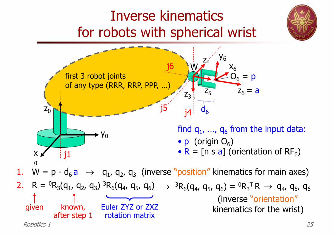
Inverse kinematics for robots with spherical wrist

x0

y0

z0

x6

y6

z6 = a

first 3 robot jointsof any type (RRR, RRP, PPP, …)

find q1, …, q6 from the input data:• p (origin O6)• R = [n s a] (orientation of RF6)

z3z5

j4j5

j6O6 = p

W

d6

j1

1. W = p - d6 a ® q1, q2, q3 (inverse “position” kinematics for main axes)

2. R = 0R3(q1, q2, q3) 3R6(q4, q5, q6)

(inverse “orientation” kinematics for the wrist)given Euler ZYZ or ZXZ

rotation matrixknown,

after step 1

® 3R6(q4, q5, q6) = 0R3T R

Robotics 1 25

z4

® q4, q5, q6

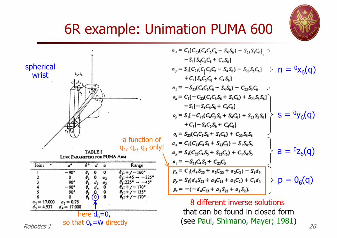
6R example: Unimation PUMA 600

8 different inverse solutions that can be found in closed form(see Paul, Shimano, Mayer; 1981)

sphericalwrist

Robotics 1 26

a = 0z6(q)

n = 0x6(q)

s = 0y6(q)

p = 06(q)

here d6=0, so that 06=W directly

a function ofq1, q2, q3 only!

¬ neglected

n use when a closed-form solution q to rd = fr(q) does not exist or is “too hard” to be found

n (analytical Jacobian)

n Newton method (here for m=n)n rd = fr(q) = fr(qk) + Jr(qk) (q - qk) + o(║q - qk║2)

qk+1 = qk + Jr-1(qk) [rd - fr(qk)]

n convergence if q0 (initial guess) is close enough to some q*: fr(q*) = rdn problems near singularities of the Jacobian matrix Jr(q) n in case of robot redundancy (m<n), use the pseudo-inverse Jr

#(q) n has quadratic convergence rate when near to solution (fast!)

Numerical solution of inverse kinematics problems

Jr(q) = ¶fr¶q

Robotics 1 27

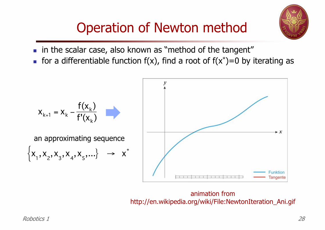
Operation of Newton method

n in the scalar case, also known as “method of the tangent”

n for a differentiable function f(x), find a root of f(x*)=0 by iterating as

Robotics 1 28

animation from

http://en.wikipedia.org/wiki/File:NewtonIteration_Ani.gif

an approximating sequence

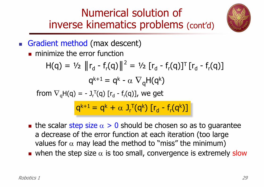
n Gradient method (max descent)n minimize the error function

H(q) = ½ ║rd - fr(q)║2 = ½ [rd - fr(q)]T [rd - fr(q)]

qk+1 = qk - a ÑqH(qk)from ÑqH(q) = - Jr

T(q) [rd - fr(q)], we get

qk+1 = qk + a JrT(qk) [rd - fr(qk)]

n the scalar step size a > 0 should be chosen so as to guarantee a decrease of the error function at each iteration (too large values for a may lead the method to “miss” the minimum)

n when the step size a is too small, convergence is extremely slow

Numerical solution of inverse kinematics problems (cont’d)

Robotics 1 29

Revisited as a “feedback” scheme

JrT(q) ó

õ

fr(q)

+

-

erd q.q

q(0)

rd = cost

e = rd - fr(q) ® 0 Û closed-loop equilibrium e=0 is asymptotically stable

V = ½ eTe ³ 0 Lyapunov candidate function.q

.e

.V = eT = eT d (

dt(rd - fr(q)) = - eT Jr = - eT Jr Jr

Te £ 0.V = 0 Û e Î Ker(Jr

T) in particular e = 0

asymptotic stability

(a = 1)

Robotics 1 30

r

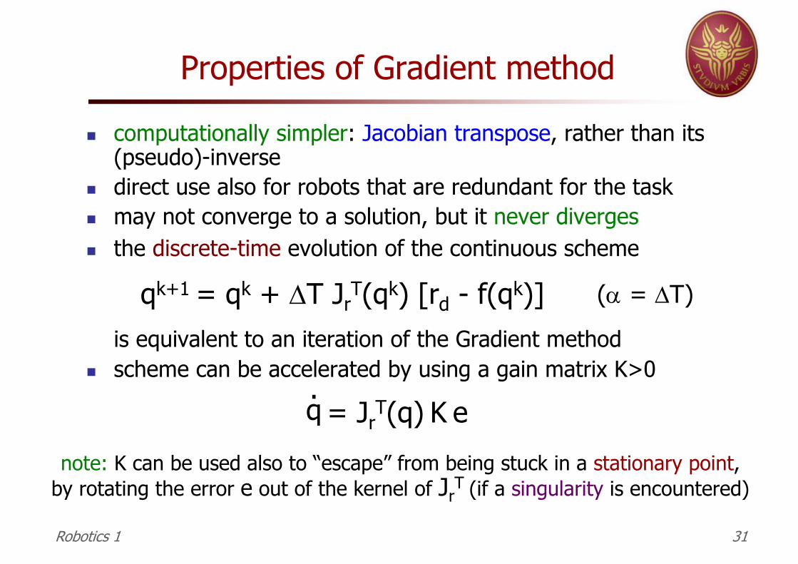
Properties of Gradient method

n computationally simpler: Jacobian transpose, rather than its (pseudo)-inverse

n direct use also for robots that are redundant for the taskn may not converge to a solution, but it never divergesn the discrete-time evolution of the continuous scheme

is equivalent to an iteration of the Gradient methodn scheme can be accelerated by using a gain matrix K>0

.q = Jr

T(q) K e

qk+1 = qk + DT JrT(qk) [rd - f(qk)] (a = DT)

note: K can be used also to “escape” from being stuck in a stationary point,by rotating the error e out of the kernel of Jr

T (if a singularity is encountered)

Robotics 1 31

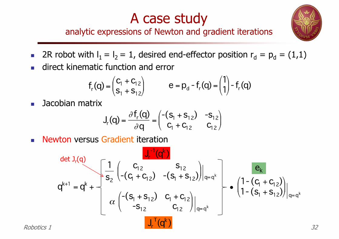
A case studyanalytic expressions of Newton and gradient iterations

n 2R robot with l1 = l2 = 1, desired end-effector position rd = pd = (1,1)n direct kinematic function and error

n Jacobian matrix

n Newton versus Gradient iteration

Robotics 1 32

•

ek

det Jr(q)

Error functionn 2R robot with l1=l2=1, desired end-effector position pd = (1,1)

Robotics 1 33

plot of ║e║2 as a function of q = (q1,q2)

e = pd - fr(q)

two local minima(inverse kinematic solutions)

Error reduction by Gradient methodn flow of iterations along the negative (or anti-) gradientn two possible cases: convergence or stuck (at zero gradient)

Robotics 1 34

start

one solution

local maximum(stop if this is the initial guess)

. .

another start...

...the other solution

saddle point(stop after some iterations)

(q1,q2)’ =(0,π/2) (q1,q2)” =(π/2,-π/2) (q1,q2)max =(-3π/4,0) (q1,q2)saddle =(π/4,0)

e Î Ker(JrT) !

Convergence analysiswhen does the gradient method get stuck?

n lack of convergence occurs whenn the Jacobian matrix Jr(q) is singular (the robot is in a “singular configuration”)n AND the error is in the “null space” of Jr

T(q)

Robotics 1 35

(q1,q2)max =(-3π/4,0)

(q1,q2)saddle =(π/4,0) e Î Ker(JrT)

pd

p

q1

q2

e ∉ Ker(JrT) !!

pd

p

e Î Ker(JrT)

pd

p

(q1,q2) =(π/9,0)

the algorithm will proceed in this case,

moving out ofthe singularity

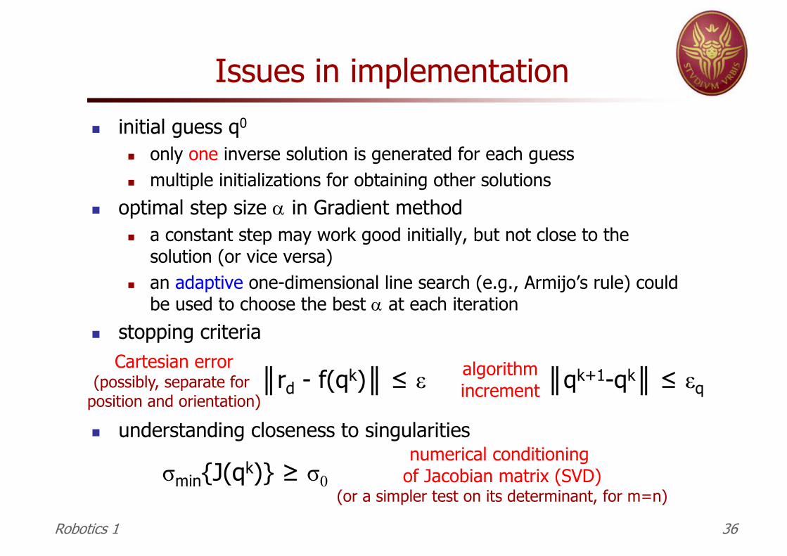
Issues in implementationn initial guess q0

n only one inverse solution is generated for each guessn multiple initializations for obtaining other solutions

n optimal step size a in Gradient methodn a constant step may work good initially, but not close to the

solution (or vice versa)n an adaptive one-dimensional line search (e.g., Armijo’s rule) could

be used to choose the best a at each iterationn stopping criteria

n understanding closeness to singularities

║qk+1-qk║ ≤ εq║rd - f(qk)║ ≤ εCartesian error

(possibly, separate for position and orientation)

algorithmincrement

σmin{J(qk)} ≥ σ0numerical conditioning

of Jacobian matrix (SVD)(or a simpler test on its determinant, for m=n)

Robotics 1 36

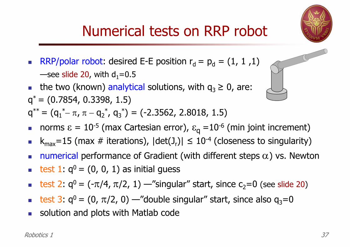
Numerical tests on RRP robot

n RRP/polar robot: desired E-E position rd = pd = (1, 1 ,1) —see slide 20, with d1=0.5

n the two (known) analytical solutions, with q3 ≥ 0, are:q* = (0.7854, 0.3398, 1.5)q** = (q1

*- p, p - q2*, q3

*) = (-2.3562, 2.8018, 1.5)

n norms ε = 10-5 (max Cartesian error), εq =10-6 (min joint increment)n kmax=15 (max # iterations), |det(Jr)| ≤ 10-4 (closeness to singularity)

n numerical performance of Gradient (with different steps a) vs. Newtonn test 1: q0 = (0, 0, 1) as initial guess

n test 2: q0 = (-p/4, p/2, 1) —”singular” start, since c2=0 (see slide 20)

n test 3: q0 = (0, p/2, 0) —”double singular” start, since also q3=0n solution and plots with Matlab code

Robotics 1 37

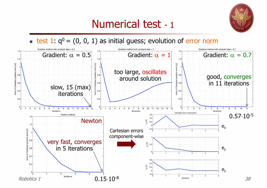
Numerical test - 1

n test 1: q0 = (0, 0, 1) as initial guess; evolution of error norm

Robotics 1 38

Gradient: a = 0.5 Gradient: a = 1 Gradient: a = 0.7

slow, 15 (max)iterations

too large, oscillatesaround solution good, converges

in 11 iterations

Newton

very fast, convergesin 5 iterations

0.15⋅10-8

0.57⋅10-5

Cartesian errorscomponent-wise

ex

ey

ez

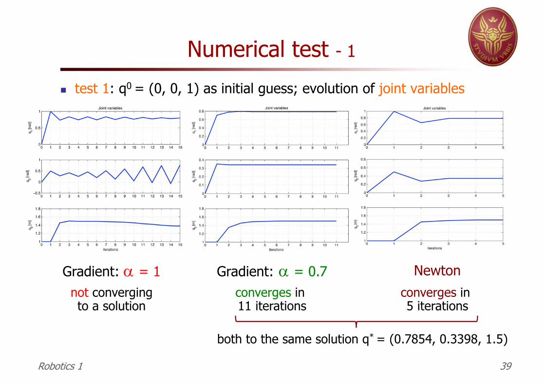
Numerical test - 1

n test 1: q0 = (0, 0, 1) as initial guess; evolution of joint variables

Robotics 1 39

Gradient: a = 1 Gradient: a = 0.7not convergingto a solution

converges in 11 iterations

Newtonconverges in 5 iterations

both to the same solution q* = (0.7854, 0.3398, 1.5)

Numerical test - 2

n test 2: q0 = (-p/4, p/2, 1): singular start

Robotics 1 40

Gradienta = 0.7

with check of singularity:

blocked at start

without check:it diverges!

Newton

erro

r nor

ms

starts towardsolution, butslowly stops

(in singularity):when Cartesian errorvector e ∈ Ker(Jr

T) join

t var

iabl

es

!!

Numerical test - 3

n test 3: q0 = (0, p/2, 0): “double” singular start

Robotics 1 41

Newtonis either

blocked at startor (w/o check)

explodes!→ “NaN” in Matlab

erro

r no

rm

Gradient (with a = 0.7)� starts toward solution� exits the double singularity� slowly converges in 19

iterations to the solutionq*=(0.7854, 0.3398, 1.5)

join

t va

riab

les

Car

tesi

an e

rror

s

�

�

�

0.96⋅10-5

Final remarks

n an efficient iterative scheme can be devised by combiningn initial iterations using Gradient (“sure but slow”, linear convergence rate)n switch then to Newton method (quadratic terminal convergence rate)

n joint range limits are considered only at the endn check if the solution found is feasible, as for analytical methods

n in alternative, an optimization criterion can be included in the search n driving iterations toward an inverse kinematic solution with nicer properties

n if the problem has to be solved on-linen execute iterations and associate an actual robot motion: repeat steps at

times t0, t1=t0+T, ..., tk=tk-1+T (e.g., every T=40 ms)

n the “good” choice for the initial guess q0 at tk is the solution of the previous problem at tk-1 (provides continuity, needs only 1-2 Newton iterations)

n crossing of singularities/handling of joint range limits need special care

n Jacobian-based inversion schemes are used also for kinematic control, along a continuous task trajectory rd(t)

Robotics 1 42