Productivity and the New Zealand Dollar: Balassa-Samuelson ... · Productivity and the New Zealand...

Productivity and the New Zealand Dollar: Balassa-Samuelson tests on sectoral data

AN 2013/01

Daan Steenkamp

June 2013

Reserve Bank of New Zealand Analytical Note series

ISSN 2230-5505

Reserve Bank of New Zealand PO Box 2498 Wellington

NEW ZEALAND

www.rbnz.govt.nz

The Analytical Note series encompasses a range of types of background papers prepared by Reserve Bank staff. Unless otherwise stated, views expressed are those of the authors, and do

not necessarily represent the views of the Reserve Bank.

http://www.rbnz.govt.nz/

Reserve Bank of New Zealand Analytical Note Series 2 _____________________________________________________________

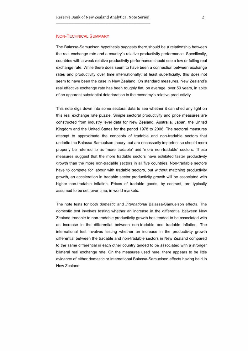
NON-TECHNICAL SUMMARY The Balassa-Samuelson hypothesis suggests there should be a relationship between

the real exchange rate and a country’s relative productivity performance. Specifically,

countries with a weak relative productivity performance should see a low or falling real

exchange rate. While there does seem to have been a connection between exchange

rates and productivity over time internationally; at least superficially, this does not

seem to have been the case in New Zealand. On standard measures, New Zealand’s

real effective exchange rate has been roughly flat, on average, over 50 years, in spite

of an apparent substantial deterioration in the economy’s relative productivity.

This note digs down into some sectoral data to see whether it can shed any light on

this real exchange rate puzzle. Simple sectoral productivity and price measures are

constructed from industry level data for New Zealand, Australia, Japan, the United

Kingdom and the United States for the period 1978 to 2006. The sectoral measures

attempt to approximate the concepts of tradable and non-tradable sectors that

underlie the Balassa-Samuelson theory, but are necessarily imperfect so should more

properly be referred to as ‘more tradable’ and ‘more non-tradable’ sectors. These

measures suggest that the more tradable sectors have exhibited faster productivity

growth than the more non-tradable sectors in all five countries. Non-tradable sectors

have to compete for labour with tradable sectors, but without matching productivity

growth, an acceleration in tradable sector productivity growth will be associated with

higher non-tradable inflation. Prices of tradable goods, by contrast, are typically

assumed to be set, over time, in world markets.

The note tests for both domestic and international Balassa-Samuelson effects. The

domestic test involves testing whether an increase in the differential between New

Zealand tradable to non-tradable productivity growth has tended to be associated with

an increase in the differential between non-tradable and tradable inflation. The

international test involves testing whether an increase in the productivity growth

differential between the tradable and non-tradable sectors in New Zealand compared

to the same differential in each other country tended to be associated with a stronger

bilateral real exchange rate. On the measures used here, there appears to be little

evidence of either domestic or international Balassa-Samuelson effects having held in

New Zealand.


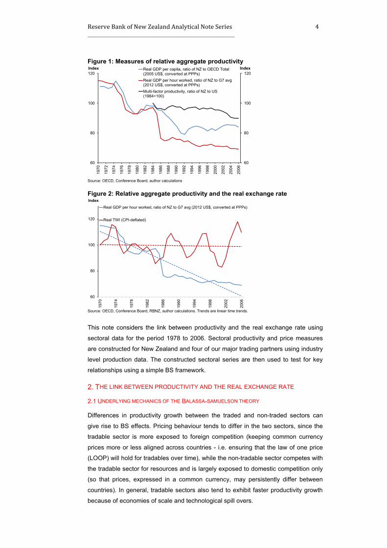
1. INTRODUCTION This note examines the longer-run relationship between New Zealand’s productivity

performance and the real exchange rate. Over recent decades, a substantial

aggregate productivity gap has opened up between New Zealand and other advanced

economies (Figure 1). All other things equal, the BS hypothesis suggests that such a

divergence in relative productivity should drive down the real exchange rate over the

long-term (i.e. once cyclical factors like house price fluctuations or slow price

adjustment can be abstracted from).1 But Figure 2 suggests that there has been no

positive relationship between various measures of relative productivity and the

Reserve Bank’s real trade-weighted index (TWI) measure of the real exchange rate

over this horizon. Empirical tests tend to struggle to find a statistically significant and

positive relationship between aggregate productivity and the real exchange rate in

New Zealand. 2 It is puzzling that the real exchange rate has, over the long-term,

resisted the apparent deterioration in the economy’s underlying competitiveness.

The BS hypothesis is often used to explain deviations from what the theory of

Purchasing Power Parity (PPP) would otherwise suggest for the evolution of the real

exchange rate. 3 The BS hypothesis suggests that relative productivity differences

between countries, and changes in relative productivity over time, will affect the real

exchange rate. This is because measures of the real exchange rate reflect relative

national price levels – which comprise prices in the traded and non-traded sectors –

across countries. If productivity growth accelerates in a country’s tradables sector –

whose product prices are determined internationally – activity in that sector will

expand and, in competition with non-tradables sector firms, real wages will be bid up

across the economy. All else equal, that will tend to raise prices in the non-tradable

sector relative to those in the tradable sector, raising that country’s real exchange

rate. If, on the other hand, productivity growth in a country’s tradable sector lags,

there will be less competition for resources in the non-tradable sector, and the real

exchange rate will tend to weaken. Section 2 and Box 1 explain the mechanics in

more detail.

1 See seminal papers by Balassa (1964) and Samuelson (1964). 2 Updating the Dynamic OLS results from Brook and Hargreaves (2001) provides some evidence of a positive relationship between various productivity proxies and the real bilateral exchanges rate between New Zealand and Australia, Japan and the UK, provided terms of trade are controlled for. No productivity proxies are significant for the comparison with the US. Most of the specifications tested however still had serial correlation in their residuals, so the autoregressive distributed lag approach of Pesaran and Shin (1999) and Pesaran et al (2001) was also considered. This approach can be used irrespective of the order of integration of the variables in the model and can improve efficiency in small samples relative to VAR approaches. Based on this approach, there is evidence of cointegration between the real exchange rate, relative productivity and relative terms of trade for the bilaterals with the US, Japan and the UK, but not Australia. Relative productivity is only significant in the regressions for Japan and the UK. In a dynamic panel setting using a sample running from 1973 to 2008, Chong, Jordà and Taylor (2012) find that there is support for the BS effect globally, although for New Zealand the effect is small and statistically insignificant (negative when the US is used as numeraire and positive when the sample average is used as reference). 3 Over the long-term, PPP suggests that aggregate price levels, expressed in a common currency, should be roughly equal across countries (known as absolute PPP). Likewise, PPP implies that the exchange rate should adjust to cross-country inflation differentials over time (known as relative PPP).


Figure 1: Measures of relative aggregate productivity

Source: OECD, Conference Board, author calculations

Figure 2: Relative aggregate productivity and the real exchange rate

Source: OECD, Conference Board, RBNZ, author calculations. Trends are linear time trends.

This note considers the link between productivity and the real exchange rate using

sectoral data for the period 1978 to 2006. Sectoral productivity and price measures

are constructed for New Zealand and four of our major trading partners using industry

level production data. The constructed sectoral series are then used to test for key

relationships using a simple BS framework.

2. THE LINK BETWEEN PRODUCTIVITY AND THE REAL EXCHANGE RATE

2.1 UNDERLYING MECHANICS OF THE BALASSA-SAMUELSON THEORY Differences in productivity growth between the traded and non-traded sectors can

give rise to BS effects. Pricing behaviour tends to differ in the two sectors, since the

tradable sector is more exposed to foreign competition (keeping common currency

prices more or less aligned across countries - i.e. ensuring that the law of one price

(LOOP) will hold for tradables over time), while the non-tradable sector competes with

the tradable sector for resources and is largely exposed to domestic competition only

(so that prices, expressed in a common currency, may persistently differ between

countries). In general, tradable sectors also tend to exhibit faster productivity growth

because of economies of scale and technological spill overs.

1970

1972

1974

1976

1978

1980

1982

1984

1986

1988

1990

1992

1994

1996

1998

2000

2002

2004

2006

60

80

100

120

60

80

100

120IndexIndex Real GDP per capita, ratio of NZ to OECD Total

(2005 US$, converted at PPPs)Real GDP per hour worked, ratio of NZ to G7 avg(2012 US$, converted at PPPs)Multi-factor productivity, ratio of NZ to US(1984=100)

60

80

100

120

1970

1974

1978

1982

1986

1990

1994

1998

2002

2006

IndexReal GDP per hour worked, ratio of NZ to G7 avg (2012 US$, converted at PPPs)

Real TWI (CPI-deflated)


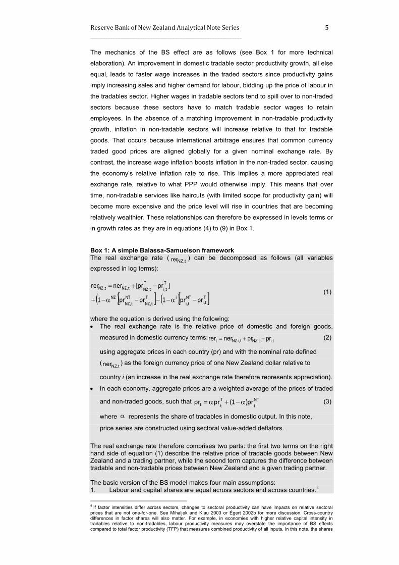
The mechanics of the BS effect are as follows (see Box 1 for more technical

elaboration). An improvement in domestic tradable sector productivity growth, all else

equal, leads to faster wage increases in the traded sectors since productivity gains

imply increasing sales and higher demand for labour, bidding up the price of labour in

the tradables sector. Higher wages in tradable sectors tend to spill over to non-traded

sectors because these sectors have to match tradable sector wages to retain

employees. In the absence of a matching improvement in non-tradable productivity

growth, inflation in non-tradable sectors will increase relative to that for tradable

goods. That occurs because international arbitrage ensures that common currency

traded good prices are aligned globally for a given nominal exchange rate. By

contrast, the increase wage inflation boosts inflation in the non-traded sector, causing

the economy’s relative inflation rate to rise. This implies a more appreciated real

exchange rate, relative to what PPP would otherwise imply. This means that over

time, non-tradable services like haircuts (with limited scope for productivity gain) will

become more expensive and the price level will rise in countries that are becoming

relatively wealthier. These relationships can therefore be expressed in levels terms or

in growth rates as they are in equations (4) to (9) in Box 1.

Box 1: A simple Balassa-Samuelson framework The real exchange rate ( t,NZrer ) can be decomposed as follows (all variables

expressed in log terms):

( )[ ] ( )[ ]Tt,i

NTt,i

iTt,NZ

NTt,NZ

NZ

Tt,i

Tt,NZt,NZt,NZ

prpr1prpr1

]prpr[nerrer

−α−−−α−+

−+= (1)

where the equation is derived using the following: • The real exchange rate is the relative price of domestic and foreign goods,

measured in domestic currency terms: t,it,NZt,i:NZt prprnerrer −+= (2)

using aggregate prices in each country (pr) and with the nominal rate defined

( t,NZner ) as the foreign currency price of one New Zealand dollar relative to

country i (an increase in the real exchange rate therefore represents appreciation).

• In each economy, aggregate prices are a weighted average of the prices of traded

and non-traded goods, such that NTt

Ttt pr)1(prpr α−+α= (3)

where α represents the share of tradables in domestic output. In this note,

price series are constructed using sectoral value-added deflators.

The real exchange rate therefore comprises two parts: the first two terms on the right hand side of equation (1) describe the relative price of tradable goods between New Zealand and a trading partner, while the second term captures the difference between tradable and non-tradable prices between New Zealand and a given trading partner.

The basic version of the BS model makes four main assumptions: 1. Labour and capital shares are equal across sectors and across countries.4

4 If factor intensities differ across sectors, changes to sectoral productivity can have impacts on relative sectoral prices that are not one-for-one. See Mihaljek and Klau 2003 or Égert 2002b for more discussion. Cross-country differences in factor shares will also matter. For example, in economies with higher relative capital intensity in tradables relative to non-tradables, labour productivity measures may overstate the importance of BS effects compared to total factor productivity (TFP) that measures combined productivity of all inputs. In this note, the shares


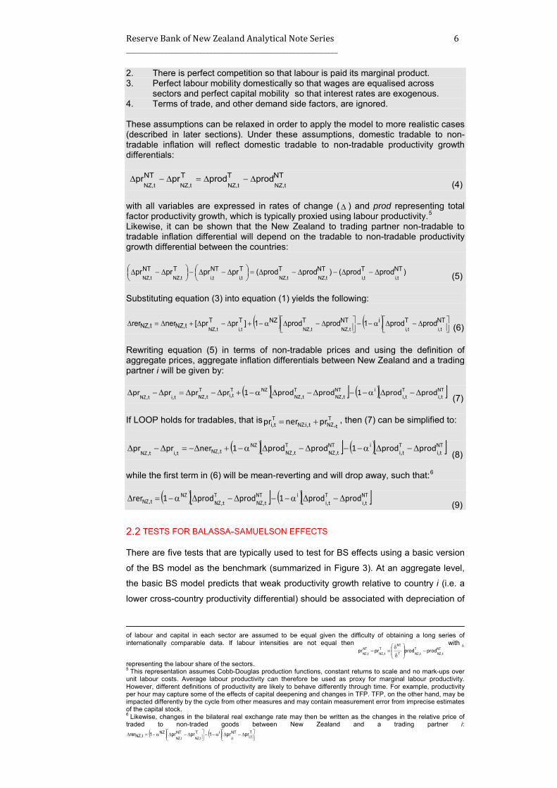
2. There is perfect competition so that labour is paid its marginal product. 3. Perfect labour mobility domestically so that wages are equalised across sectors and perfect capital mobility so that interest rates are exogenous. 4. Terms of trade, and other demand side factors, are ignored. These assumptions can be relaxed in order to apply the model to more realistic cases (described in later sections). Under these assumptions, domestic tradable to non-tradable inflation will reflect domestic tradable to non-tradable productivity growth differentials: NTTTNT

t,NZt,NZt,NZt,NZprodprodprpr ∆−∆=∆−∆

(4) with all variables are expressed in rates of change (∆ ) and prod representing total factor productivity growth, which is typically proxied using labour productivity.5 Likewise, it can be shown that the New Zealand to trading partner non-tradable to tradable inflation differential will depend on the tradable to non-tradable productivity growth differential between the countries:

)prodprod()prodprod(prprprpr NTTNTTTNTTNTt,it,it,NZt,NZt,it,it,NZt,NZ

∆−∆−∆−∆=

∆−∆−

∆−∆

(5)

Substituting equation (3) into equation (1) yields the following:

( ) ( )

∆−∆α−−

∆−∆α−+∆−∆+∆=∆ NTTiNTTNZTT

t,NZt,NZ t,it,it,NZt,NZt,it,NZprodprod1prodprod1]prpr[nerrer

(6) Rewriting equation (5) in terms of non-tradable prices and using the definition of aggregate prices, aggregate inflation differentials between New Zealand and a trading partner i will be given by:

( )[ ] ( )[ ]NTt,i

Tt,i

iNTt,NZ

Tt,NZ

NZTt,i

Tt,NZt,it,NZ

prodprod1prodprod1prprprpr ∆−∆α−−∆−∆α−+∆−∆=∆−∆ (7)

If LOOP holds for tradables, that is T

t,NZt,i:NZTt,i prnerpr += , then (7) can be simplified to:

(8) while the first term in (6) will be mean-reverting and will drop away, such that:6

( )[ ] ( )[ ]NTt,i

Tt,i

iNTt,NZ

Tt,NZ

NZt,NZ prodprod1prodprod1rer ∆−∆α−−∆−∆α−=∆

(9)

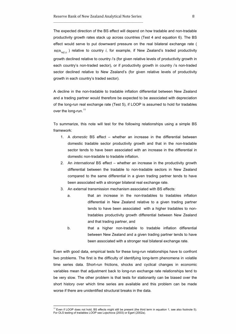
2.2 TESTS FOR BALASSA-SAMUELSON EFFECTS There are five tests that are typically used to test for BS effects using a basic version

of the BS model as the benchmark (summarized in Figure 3). At an aggregate level,

the basic BS model predicts that weak productivity growth relative to country i (i.e. a

lower cross-country productivity differential) should be associated with depreciation of

of labour and capital in each sector are assumed to be equal given the difficulty of obtaining a long series of internationally comparable data. If labour intensities are not equal then

NTt,NZ

Tt,NZT

NTT

t,NZNT

t,NZ prodprodprpr −

δδ

=− with δ

representing the labour share of the sectors. 5 This representation assumes Cobb-Douglas production functions, constant returns to scale and no mark-ups over unit labour costs. Average labour productivity can therefore be used as proxy for marginal labour productivity. However, different definitions of productivity are likely to behave differently through time. For example, productivity per hour may capture some of the effects of capital deepening and changes in TFP. TFP, on the other hand, may be impacted differently by the cycle from other measures and may contain measurement error from imprecise estimates of the capital stock. 6 Likewise, changes in the bilateral real exchange rate may then be written as the changes in the relative price of traded to non-traded goods between New Zealand and a trading partner i:

( ) ( )

∆−∆α−−

∆−∆α−=∆ T

t,iNTiTNTNZ

t,NZ prpr1prpr1rert,it,NZt,NZ

( )[ ] ( )[ ]NTt,i

Tt,i

iNTt,NZ

Tt,NZ

NZt,NZt,it,NZ

prodprod1prodprod1nerprpr ∆−∆α−−∆−∆α−+∆−=∆−∆


the real bilateral exchange rate (Test 1).7 Figure 2 suggests that this has not held in

New Zealand’s case.

The predicted aggregate relationship depends on implied relationships between

sectoral inflation and productivity differentials and the real exchange rate. The basic

model assumes that the domestic differential between non-tradable to tradable

inflation ( Tt,NZ

PR∆ less NTt,NZ

PR∆ ) reflects the differential between relative productivity

growth between the two sectors ( Tt,NZ

PROD∆ over NTt,NZ

PROD∆ ) (Test 2 using equation

4 in Box 1). This is sometimes called the domestic test of the BS effect.8

The external transmission mechanism of the BS effect relies on the assumption that a

country’s tradable to non-tradable productivity growth differential with different trading

partners are responsible for observed bilateral non-tradable to tradable inflation

differentials (Test 3 and equation 5).9 Said differently, this supposes that the domestic

BS relationship holds across trading partners – if the gap between New Zealand’s

tradable and non-tradable productivity increase relative to that in another country we

would also expect to see the gap between New Zealand’s tradable and non-tradable

inflation relative to that other country increase.10

Figure 3: Simple tests for BS effects

7 See, for example, Balassa (1964) or De Broeck and Slok (2001) in a cross-sectional setting, Alquist and Chinn (2002) in a time series cointegration setting, Drine and Rault (2005) in a panel context or Chowdhury (2011) for an ARDL application. 8 This is also sometimes referred to as the Baumol and Bowen (1966) effect. Productivity is expected to rise more slowly in service sectors, which tend to have higher labour intensity than the manufacturing sector. See Mihaljek and Klau (2003, 2008) for more detail. 9 See Égert (2002a) or (2002b) for examples. 10 Some studies proceed directly to testing whether bilateral inflation differentials can be explained by relative sectoral productivity differentials (i.e. using equation 7 or 8). See OLS studies by Lojschova 2003 or Mihaljek and Klau (2003, 2008). The latter also include a lagged dependent variable to deal with autocorrelation. Drine and Rault (2005) use only relative sectoral productivities and apply Johansen’s cointegration approach in a panel setting.

4

Aggregate Productivity Test

Sectoral Productivity - Prices Test

Sectoral Productivity Test1

5

Real bilateral exchange rate depreciates

Sectoral productivity differentials and sectoral price differentials

3

2

Domestic BS effect

International BS effect

∆

∆

∆

∆

NT

T

NT

T

i

i

NZ

NZ

PROD

PROD

PROD

PROD

i

NZoductivityPr

oductivityPr∆∆

NT

T

T

NT

i

i

i

i

PROD

PROD

PR

PR

∆

∆=

∆

∆

∆

∆

∆

∆

T

NT

T

NT

i

i

NZ

NZ

PR

PR

PR

PR

t,i:NZRER∆


The expected direction of the BS effect will depend on how tradable and non-tradable

productivity growth rates stack up across countries (Test 4 and equation 6). The BS

effect would serve to put downward pressure on the real bilateral exchange rate (

t,i:NZRER ) relative to country i, for example, if New Zealand’s traded productivity

growth declined relative to country i’s (for given relative levels of productivity growth in

each country’s non-traded sector), or if productivity growth in country i’s non-traded

sector declined relative to New Zealand’s (for given relative levels of productivity

growth in each country’s traded sector).

A decline in the non-tradable to tradable inflation differential between New Zealand

and a trading partner would therefore be expected to be associated with depreciation

of the long-run real exchange rate (Test 5), if LOOP is assumed to hold for tradables

over the long-run.11

To summarize, this note will test for the following relationships using a simple BS

framework:

1. A domestic BS effect – whether an increase in the differential between

domestic tradable sector productivity growth and that in the non-tradable

sector tends to have been associated with an increase in the differential in

domestic non-tradable to tradable inflation.

2. An international BS effect – whether an increase in the productivity growth

differential between the tradable to non-tradable sectors in New Zealand

compared to the same differential in a given trading partner tends to have

been associated with a stronger bilateral real exchange rate.

3. An external transmission mechanism associated with BS effects:

a. that an increase in the non-tradables to tradables inflation

differential in New Zealand relative to a given trading partner

tends to have been associated with a higher tradables to non-

tradables productivity growth differential between New Zealand

and that trading partner, and

b. that a higher non-tradable to tradable inflation differential

between New Zealand and a given trading partner tends to have

been associated with a stronger real bilateral exchange rate.

Even with good data, empirical tests for these long-run relationships have to confront

two problems. The first is the difficulty of identifying long-term phenomena in volatile

time series data. Short-run frictions, shocks and cyclical changes in economic

variables mean that adjustment back to long-run exchange rate relationships tend to

be very slow. The other problem is that tests for stationarity can be biased over the

short history over which time series are available and this problem can be made

worse if there are unidentified structural breaks in the data.

11 Even if LOOP does not hold, BS effects might still be present (the third term in equation 1, see also footnote 5). For OLS testing of tradables LOOP see Lojschova (2003) or Egert (2002a).


To address these problems, studies tend to opt for methodologies that use low

frequency time series or panel data to help improve the power of econometric tests.

Over recent years, cointegration techniques using higher frequency data have also

become popular in identifying long-run relationships between real exchange rates, BS

effects and other determinants of exchange rates. Given the short sample for which

data are available, the analysis here relies on the simple decomposition of the real

exchange rate outlined in Box 1 and some simple regressions.

3. DATA Getting good quality data to test for BS relationships is itself a challenge. Comparable

tradable and non-tradable measures for New Zealand and Australia, Japan, the

United Kingdom and the United States are constructed using sectoral output and

labour-input measures. In the absence of long series of internationally comparable

total factor productivity measures or data on hours worked, productivity is proxied

using output per worker. This is calculated as real value-added divided by total

number engaged using data from the OECD’s STAN database, which has data

available for New Zealand from 1977 to 2006. To obtain long series of New Zealand

industry level employment data, unofficial backdated series were obtained from

Statistics New Zealand. These series only go back to 1978 and are used for the full

sample – which is from 1978 to 2006.12 All series used are annual and are re-indexed

to a 1978 base year (1989 when comparing New Zealand and Australia since

Australian sectoral employment data is not available prior to that in the STAN

database).

It is also difficult to accurately separate tradable and non-tradable sectors.13 In the

main text, manufacturing plus agriculture and mining are together taken to represent

the tradable sector and total services plus construction and electricity are used to

represent the non-tradables sector. The labelling of services as non-tradables can be

quite problematic. For example, a substantial portion of New Zealand’s tourism and

education exports are captured as services and in the UK financial services make up

a substantial share of total exports.14 Because these categorisations are necessarily

imperfect, sectors should more properly be referred to as ‘more tradable’ and ‘more

non-tradable’.

In the Appendix, results are also presented using a narrower classification scheme

(Classification 2), in which the traded sector is represented as as manufacturing only,

while services are taken to represent non-tradables.

12 There are several caveats around the unofficial sector employment series used, which mean that these figures have not been completely quality assured by Statistics New Zealand. 13 Both tradable and non-tradable products and services will include intermediate inputs from the other sector and the share of tradable components in the aggregate output might have varied over time. 14 In the STAN database, services comprise wholesale and retail trade, restaurants and hotels; transport, storage and communications; finance, insurance, real estate and business services; community, social and personal services.


It is quite common to see discussion of tradables and non-tradables inflation drawing

on components of the Consumer Price Index (CPI) because of their international

comparability. Unfortunately, CPI-based measures of tradables and non-tradables are

not available for all the countries of interest for a sufficiently long sample. Sectoral

value-added deflators, on the other hand, are useful as they capture all production in

different sectors of the economy, though they will not capture import prices. In this

note, value-added deflators are used to calculate all price series to ensure

consistency in the measurement of productivity growth and sectoral inflation. 15

Likewise, all real exchange rates used for formal empirical work are computed on the

basis of value-added deflators.

Aggregate price series are created by using sectoral deflators and by weighting

tradables and non-tradables by their volume value-added shares in total output, as in

equation (3) in Box 1. The share of tradables in total output for each country, α in

equation (1), is calculated using the average values of α during the period 1978 to

2006, except Australia (where 1989 to 2006 is used). This yields an average tradable

share of 23 percent in the first classification and 21 percent in the second.16

Figure 4 shows that, for New Zealand and Australia, using a value-added definition of

sectoral prices produces very different inflation measures than those based on

consumer prices, especially for tradable prices. This distinction is particularly

important in the Australian case, where the high rate of tradables sector inflation

reflects the strong increase in the country’s commodity export prices over the period

(which has little direct bearing on general Australian consumer prices).

15 Producer prices could instead be used to capture tradables prices and consumer prices instead used to proxy non-tradables prices. Under the narrow sector classification 2, for example, over recent history tradable real bilateral exchange rates (

t,NZner + Tt,NZpr - T

t,ipr ) would be more appreciated against all four currencies. Relative non-tradable

prices ( )[ ] ( )[ ]Tt,i

NTt,i

iTt,NZ

NTt,NZ

NZ prpr1prpr1 −α−−−α− , on the other hand, would be higher compared to the US and UK

and lower for Japan and AU over recent history. Note also that using different measures of sector prices would give different weight to non-tradables in domestic prices. In Engel (1999), for example, the contribution to the price index of non-tradables is higher when using output series than when using CPI-based measures. 16 The use of sample averages to weight the sectors does not fully capture the decline in the share of manufacturing in production in Australia, the UK and New Zealand over the sample. Alternative weighting schemes were also considered: the first uses each country’s average tradable sector share over the sample (which yields US=0.17, JP=0.24,UK=0.24, NZ=0.27, AU=0.22 for classification 1, US=0.16, JP=0.25,UK=0.22, NZ=0.22, AU=0.16 for classification 2), while the second uses each country’s period by period shares of manufacturing to total value added. When changes in these shares through time are taken into account, the international BS effects are slightly larger, but this does not affect judgements about the relevance of BS effects. Note that the STAN data do not provide the unallocated components of production GDP or FISM for all countries considered so combined sectoral output does not equal total GDP. This makes is difficult to calculate the coverage of each classification scheme. The first scheme accounts for close to, but probably a little less than, full coverage, while the narrower classification covers roughly 80 percent of total output in all countries under consideration.


Figure 4: CPI- versus value-added deflator-based inflation (1999 – 2006)*

* The period selected reflects data availability.

4. SECTORAL PRODUCTIVITY AND PRICE MEASURES: SOME RESULTS This section compares how the levels of sectoral prices and productivity in New

Zealand and four of our major trading partners have changed over time. In section 5,

some of the tests from Figure 3 using prices and productivity data expressed in

growth rates are conducted.

Figure 5 compares developments in tradable and non-tradable sector productivity for

each country. In all five countries, tradable sector productivity growth has exceeded

non-tradable productivity growth. But New Zealand’s productivity growth, in both

tradable and non-tradable sectors, has been low relative to the other economies.

Figure 5: Tradable and non-tradable productivity

0

1

2

3

4

5

6

7

Tradable Non-Tradable Tradable Non-Tradable

Aver

age

annu

al p

erce

nt c

hang

e (1

999

to 2

006)

CPI-based Production-based

Australia New Zealand

-0.2

0.0

0.2

0.4

0.6

0.8

1.0

1.2

1978

1980

1982

1984

1986

1988

1990

1992

1994

1996

1998

2000

2002

2004

2006

Nat

ural

log

New Zealand

Tradables Non-tradables

-0.2

0.0

0.2

0.4

0.6

0.8

1.0

1.2

1978

1980

1982

1984

1986

1988

1990

1992

1994

1996

1998

2000

2002

2004

2006

Nat

ural

log

United States


-0.2

0.0

0.2

0.4

0.6

0.8

1.0

1.2

1978

1980

1982

1984

1986

1988

1990

1992

1994

1996

1998

2000

2002

2004

2006

Nat

ural

log

United Kingdom


-0.2

0.0

0.2

0.4

0.6

0.8

1.0

1.2

1978

1980

1982

1984

1986

1988

1990

1992

1994

1996

1998

2000

2002

2004

2006

Nat

ural

log

Japan



The BS hypothesis asserts that, over time, there is a positive relationship between

non-tradable to tradable price differentials and tradable to non-tradable productivity

growth differentials domestically, as well as across trading partners. Non-tradable to

tradable price differentials between New Zealand and the four countries considered

( )[ ] ( )[ ]Tt,i

NTt,i

iTt,NZ

NTt,NZ

NZ prpr1prpr1 −α−−−α− are plotted along with real bilateral exchange

rates (calculated using equation 1 in Box 1) in Figure 6. Here, the share of tradables

in total output for each country, alpha, is assumed to be equal for all countries.

Figure 6: Relative non-tradable to tradable price ratios (value-added measures) and real bilateral exchange rates (each with New Zealand)

The data do not permit direct comparison of level differences in common currency, so

our focus is on comparing how these measures have changed over time. To read

these, consider the US chart. The trend decline in the red line means that the gap

between tradable and non-tradable prices in the US has increased at a faster rate

over time than in New Zealand. The correlations between each country’s non-tradable

to tradable price differential with New Zealand and the bilateral real exchange rate are

positive but small in the US and Japanese cases (both 0.09), but larger in the case of

the UK (0.65) and Australia (0.53).17

17 For a large sample of OECD economies, Drozd and Nosal (2010) find that the median correlation between real exchange rates and relative non-tradable prices is 0.09 (-0.38 for the 10th percentile and 0.47 for the 90th

0.0

0.1

0.2

0.3

0.4

0.5

1978

1980

1982

1984

1986

1988

1990

1992

1994

1996

1998

2000

2002

2004

2006

Nat

ural

log

Australia


-0.4

-0.3

-0.2

-0.1

0.0

0.1

0.2

0.3

1978

1980

1982

1984

1986

1988

1990

1992

1994

1996

1998

2000

2002

2004

2006

Nat

ural

log

United States (equal alpha)

RER (value-added based)Relative NT:T ratio -0.2

-0.1

0.0

0.1

0.2

4.6

4.8

5.0

5.2

5.4

5.6

5.8

1978

1980

1982

1984

1986

1988

1990

1992

1994

1996

1998

2000

2002

2004

2006

Nat

ural

log

Nat

ural

log

Japan (equal alpha)

RER (value-added based)

Relative NT:T ratio (RHS)

-1.2

-1.0

-0.8

-0.6

-0.4

-0.2

0.0

0.2

0.4

1978

1980

1982

1984

1986

1988

1990

1992

1994

1996

1998

2000

2002

2004

2006

Nat

ural

log

United Kingdom (equal alpha)


Relative NT:T ratio

-0.4

-0.3

-0.2

-0.1

0.0

0.1

0.2

0.3

1978

1980

1982

1984

1986

1988

1990

1992

1994

1996

1998

2000

2002

2004

2006

Nat

ural

log

Australia (equal alpha)


Relative NT:T ratio


Figure 7 plots domestic non-tradable to tradable price ratios ( Tt,i

NTt,i prpr − ) against

domestic tradable to non- tradable productivity differentials ( Tt,iprod - NT

t,iprod ) for each of

the countries considered. This suggests that there may be evidence of a domestic BS

effect in the US, Japan, the UK and New Zealand. That is, in each country, prices of

non-tradables to tradables have tended to rise as the relative productivity of the

traded to the non-traded sector has risen. The correlations between the two series are

high for the US (over 0.9), Japan (over 0.9), UK (over 0.9) and New Zealand (0.89),

but negative for Australia. In Australia’s case the fall in the non-tradable to tradable

price ratio reflects its terms of trade boom starting from the mid-2000s.

Figure 7: Domestic non-tradable to tradable price ratios (value-added based) and domestic tradable to non-tradable productivity differentials

Figure 8 plots relative non-tradable to tradable price ratios between New Zealand and

each country ( ( )[ ] ( )[ ]Tt,i

NTt,i

iTt,NZ

NTt,NZ

NZ prpr1prpr1 −α−−−α− ) as well as relative productivity

differentials ( ( )[ ] ( )[ ]NTt,i

Tt,i

iNTt,NZ

Tt,NZ

NZ prodprod1prodprod1 −α−−−α− ). Relative to the US, in

particular, the behaviour of the differential between tradables and non-tradables

prices does appear to have been consistent with differences between the relative

percentile). The authors use a sample of 21 countries (210 country pairs) using annual hp-filtered (lambda = 100) data between 1970 and 2005 (deflators are also obtained from the STAN database) and a common tradable sector weight of 0.22 for all countries.

-0.2

0.0

0.2

0.4

0.6

0.8

1.0

1978

1980

1982

1984

1986

1988

1990

1992

1994

1996

1998

2000

2002

2004

2006

Nat

ural

log

New Zealand

T:NT productivity differential

NT:T price ratio

-0.2

0.0

0.2

0.4

0.6

0.8

1.0

1978

1980

1982

1984

1986

1988

1990

1992

1994

1996

1998

2000

2002

2004

2006

Nat

ural

log

United States


NT:T price ratio

-0.2

0.0

0.2

0.4

0.6

0.8

1.0

1978

1980

1982

1984

1986

1988

1990

1992

1994

1996

1998

2000

2002

2004

2006

Nat

ural

log

United Kingdom


NT:T price ratio

-0.2

0.0

0.2

0.4

0.6

0.8

1.0

1978

1980

1982

1984

1986

1988

1990

1992

1994

1996

1998

2000

2002

2004

2006

Nat

ural

log

Japan


NT:T price ratio

-0.1

0.0

0.1

0.2

1978

1980

1982

1984

1986

1988

1990

1992

1994

1996

1998

2000

2002

2004

2006

Nat

ural

log

Australia


NT:T price ratio


productivity performance of the tradable and non-tradable sectors in the two

countries. The charts show that New Zealand’s tradables to non-tradables productivity

differential has grown by less than those in Japan, the UK and the US, while New

Zealand’s non-tradables and tradables price ratio has risen by less than in Australia

(for the shorter period).

Figure 8: Relative non-tradable to tradable price ratios (value-added) and tradable to non-tradable productivity differentials (each with New Zealand)

Under the BS hypothesis, the real exchange rate is expected to depreciate if New

Zealand’s tradable sector productivity decreases relative to that in the non-tradable

sector, or if traded sector productivity decreases relative to trading partners (for given

relative levels of productivity in each country’s non-traded sector). Figure 9 plots

bilateral real exchange rates against tradable to non-tradable productivity between

New Zealand and each country ( )[ ] ( )[ ]NTt,i

Tt,i

iNTt,NZ

Tt,NZ

NZ prodprod1prodprod1 −α−−−α− . In

contrast to what the BS theory would predict, relative tradable to non-tradable

productivity differentials have not shown positive co-movement with the real bilateral

exchange rate with the US and Japan. The overall correlation between the two series

is, however, positive in the Australian case, although the correlation between the

series is only 0.17 over the period since data is first available.

Figure 9: Tradable to non-tradable productivity differentials (each with New Zealand) and real bilateral exchange rate

-0.3

-0.2

-0.1

0.0

0.1

0.2

0.3

1978

1980

1982

1984

1986

1988

1990

1992

1994

1996

1998

2000

2002

2004

2006

Nat

ural

log

United States (equal shares)

T:NT productivity differential (vs NZ)

NT:T price ratio (vs NZ)

-0.3

-0.2

-0.1

0.0

0.1

0.2

0.3

1978

1980

1982

1984

1986

1988

1990

1992

1994

1996

1998

2000

2002

2004

2006

Nat

ural

log

Japan (equal shares)



-0.3

-0.2

-0.1

0.0

0.1

0.2

0.3

1978

1980

1982

1984

1986

1988

1990

1992

1994

1996

1998

2000

2002

2004

2006

Nat

ural

log

United Kingdom (equal shares)


NT:T price ratio (vs NZ) -0.1

0.0

0.1

0.2

0.3

1978

1980

1982

1984

1986

1988

1990

1992

1994

1996

1998

2000

2002

2004

2006

Nat

ural

log

Australia (equal shares)



-0.3

-0.2

-0.1

0.0

0.1

0.2

0.3

1978

1980

1982

1984

1986

1988

1990

1992

1994

1996

1998

2000

2002

2004

2006

Nat

ural

log

United States (equal alpha)

RER (value-added based)T:NT productivity differential (vs NZ) -0.2

-0.1

0.0

0.1

4.6

4.8

5.0

5.2

5.4

5.6

5.8

1978

1980

1982

1984

1986

1988

1990

1992

1994

1996

1998

2000

2002

2004

2006

Nat

ural

log

Nat

ural

log

Japan (equal alpha)




5. TESTING THE DOMESTIC AND INTERNATIONAL TRANSMISSION CHANNELS OF BS EFFECTS Table 1 compares the growth rates of each country’s sectoral productivity and prices.

As predicted by the BS hypothesis, productivity has grown faster in the more tradable

sectors in all economies and (value-added) prices have risen faster in the more non-

tradable sectors, with the exception of Australia (especially since the early 2000s).

Both New Zealand’s domestic tradable to non-tradable productivity growth differential

and non-tradable to tradable inflation differential have been less than those in the US,

UK and Japan (Figure 10).

Table 1: Comparison of sectoral productivity growth and inflation (value-added based) (average annual percent changes)

Figure 10: Domestic non-tradable to tradable inflation (value-added based) and domestic tradable to non-tradable productivity growth differentials (1979 to 2006)

The BS hypothesis predicts a positive relationship between tradable to non-tradable

productivity differentials between trading partners and relative non-tradable to

tradable inflation differentials. Table 2 is based on equation 8 in Box 1 and

demonstrates that New Zealand’s average (value-added) inflation rate has, on

average since 1979, been higher than in the US, Japan and UK, and lower than

-1.2

-1.0

-0.8

-0.6

-0.4

-0.2

0.0

0.2

1978

1980

1982

1984

1986

1988

1990

1992

1994

1996

1998

2000

2002

2004

2006

Nat

ural

log

United Kingdom (equal alpha)

RER (value-added based)T:NT productivity differential (vs NZ)

-0.4

-0.3

-0.2

-0.1

0.0

0.1

0.2

1978

1980

1982

1984

1986

1988

1990

1992

1994

1996

1998

2000

2002

2004

2006

Nat

ural

log

Australia (equal alpha)


T:NT productivitydifferential (vs NZ)

Period Country

Inflation Tradable inflation (value-added)

(1)

Non-tradable inflation

(value-added) (2)

NT:T inflation differential (3)=(2)-(1)

(% pts)

Tradable productivity

(4)

Non-tradable productivity

(5)

T:NT productivity differential (6)=(4)-(5)

(% pts)

Australia 2.5 3.0 2.4 -0.6 2.4 1.5 0.9New Zealand 2.0 1.4 2.3 0.8 2.3 0.7 1.6United States 3.4 1.6 4.0 2.4 4.0 0.9 3.1Japan 0.7 -0.5 1.2 1.6 3.9 1.5 2.4United Kingdom 0.7 3.9 5.3 1.4 3.5 1.6 1.9New Zealand 5.7 4.8 6.2 1.4 2.3 0.5 1.8

1979 to 2006

Inflation (value-added) Productivity

1990 to 2006

0.0

0.5

1.0

1.5

2.0

2.5

3.0

3.5

Uni

ted

Stat

es

Japa

n

Uni

ted

King

dom

New

Zeal

andpe

rcen

tage

poi

nts

(ave

rage

ove

r sa

mpl

e)

Change in NT:T inflation ratio

Change in T:NT productivity differential


inflation in Australia since 1990. Relative tradable to non-tradable productivity growth

has been higher in New Zealand than in Australia, but lower than in the US, Japan

and the UK. The contribution of BS effects to bilateral (value-added) inflation

differentials is negative with the US and Japan and positive with Australia. This is

because the domestic BS effect was larger in Japan, the UK and US than in New

Zealand.

Table 2: Contribution of BS effects to (value-added based) inflation differentials compared to New Zealand (average annual percent changes)18

Table 3 summarises tests assessing whether BS effects have had a statistically

significant impact on domestic non-tradable to tradable inflation differentials for New

Zealand, the US, the UK and Japan between 1979 and 2006. Given short samples

(only 28 observations), the results from regressions should be interpreted with

caution. Tradable to non-tradable productivity growth differentials only have a

statistically significant relationship with non-tradable to tradable inflation differentials

in Japan and the United States. A one percentage point increase in the domestic

sectoral productivity differential is associated with a 0.36 percentage point increase in

domestic sectoral inflation differentials in the US, and 0.3 percentage points in Japan.

In both countries, the domestic BS effect accounts for almost half of the observed

change in the non-tradable to tradable inflation differential (though its contribution falls

when corrected for the share of the non-tradable sector).19

Finally, Table 4 shows that there has been no statistically significant relationship

between tradable to non-tradable productivity growth differentials between New

Zealand and the countries considered and changes in real bilateral exchange rates

(equations 6 and 9 in Box 1). The signs on the BS coefficients are also sensitive to

whether LOOP is assumed to hold for tradables.20

18 The assumption that LOOP holds for tradables can be relaxed (see equation 7 in Box 1), but this would not affect the value of the contribution of the BS effect in Table 2. 19 Tests of the contribution of the sectoral productivity differential to New Zealand-trading partner inflation differentials (Test 3 from Figure 2) were also carried out, but the results are not presented because they were sensitive to the approach used to deal with structural breaks in the relative inflation rate series. 20 Unit root tests do not reject null of non-stationarity for tradable prices with the US and Japan, implying that LOOP does not appear to hold across tradables for New Zealand and these two countries. Unit root tests provide some evidence, however, that tradable prices are equalised between New Zealand and the UK, over the sample.

Period CountryInflation

differential (value-added)

(1)

Change in nominal ER (inverted)

(2)

T:NT productivity growth differential

with NZ (3)

BS effect

(4)

1990 to 2006 Australia -0.5 -0.9 0.7 0.5United States 2.3 1.1 -1.3 -1.0Japan 5.0 3.1 -0.6 -0.5United Kingdom 0.8 1.2 0.0 0.0

1979 to 2006

1 is pnz - p*, 2 is an appreciation when the sign is negative, 3 is (prodTnz-prodNTnz)-(prodTi-prodNTi), 4 is (1-αNZ)(prodTnz-prodNTnz)-(1-αi)(prodTi-prodNTi).


Table 3: Estimates of the domestic BS effect

Table 4: Estimates of the BS effect on real exchange rates

To test whether the results are sensitive to the classification of sectors as tradable

and non-tradable, a second sectoral classification scheme is considered, using a

narrower definition of tradables and non-tradables as manufacturing and total

services respectively. This alternative approach raises New Zealand’s measure of

tradable inflation, lowering New Zealand’s overall non-tradable to tradable inflation

differential (see Tables A1 and A2 in the Appendix). The change also lowers the

measure of tradable sector productivity in New Zealand, causing the tradable to non-

tradable productivity differential to fall over the full sample.

The narrower classification lowers Japan’s tradable to non-tradable productivity

growth and non-tradable to tradable inflation differentials, but raises them with the UK

and the US, resulting in a larger negative value for the BS effect for these

comparisons.

Under the narrower classification, there is stronger empirical support for domestic BS

effects in the US and Japan and the BS term for the UK is significant at 10 percent

(Table A3). But tradable to non-tradable productivity growth differentials still do not

have a statistically significant relationship with non-tradable to tradable inflation in

New Zealand. And in contrast to the predicted relationship between the real exchange

rate and bilateral tradable to non-tradable productivity growth, the coefficients on beta

3 in Table A4 remain insignificant, as well as being negative against in the

regressions for the US and the UK.

BS term Contribution of T:NT productivity growth differential

to NT:T inflation differential (percentage points) (1)

Domestic BS effect (percentage points)

(2)

Country β R2

New Zealand 0.30 0.03 0.54 0.39United States 0.36** 0.20 1.09 0.90United Kingdom 0.07 0.00 0.12 0.09Japan 0.30*** 0.28 0.70 0.531 is calculated as beta times average productivity growth differential over the estimation period. 2 is calculated as the contribution variable times each country's share of non-tradables to domestic prices (here proxied using output shares). A constant is included in all regressions. Variables are in logged differences to ensure stationarity. Estimated using least squares. *, **, *** are 10, 5, 1 percent

Dependent variable: ∆pNTi,t-∆pTi,tExplanatory variables: ∆prodTi,t-∆prodNTi,t

Explanatory variables: ∆nert ∆pTnz ,t-∆pTi,t (1-αnz)∆prodNTi,t-(1-αi)∆prodTi,t

BS term

Country β1 β2 β3 R2

United States 1.02*** 1.24 0.14 0.87United Kingdom 1.01*** 1.04 0.18 0.84Japan 0.99*** 1.35* 0.31 0.86

United States -0.29 0.01United Kingdom -0.34 0.01Japan -0.11 0.00with rer calculated using the aggregate price indices weighting tradable and non-tradable prices together. A constant is included in all regressions. Variables are in logged differences to ensure stationarity. Estimated using least squares. *, **, *** are 10, 5, 1 percent significance.

Dependent variable: ∆rert

No tradables LOOP assumption

Assuming LOOP holds for tradables


5. IMPLICATIONS

Overall, this analysis suggests that changes in tradable to non-tradable productivity

have not had a material impact on changes in the ratio of non-traded to traded prices

in New Zealand or the real exchange rate over the period between 1977 and 2006. If

the data are adequately capturing the concepts used to test for BS effects, then other

factors must explain the long run behaviour of the real exchange rate. One potential

answer is that other relative prices (such as terms of trade – the ratio of export over

import prices) might have had an important influence over this horizon.21 Figure 11

plots a multilateral CPI-deflated measure of the real exchange rate and shows that

there has been a much stronger correlation between New Zealand’s terms of trade

and the real exchange rate than with economy-wide relative productivity. Future

research should relax the assumption in the basic BS model that trading partners

produce the same basket of tradable goods, and investigate the relationship between

changes in relative terms of trade and the real exchange rate.

Figure 11: Relative productivity, terms of trade and the real exchange rate

Source: OECD, Conference Board, RBNZ, authors calculations. Trends are linear time trends.

6. CONCLUSION

Productivity growth gaps between countries are expected to influence how sectoral

(non-tradable to tradable) inflation ratios move in different countries over time and

therefore how the real exchange rate behaves. The long-term deterioration in New

Zealand’s relative productivity against its major developed country peers over the last

several decades would suggest that the real exchange rate should have, all other

things equal, shown some material depreciation over this horizon.

This paper tested this notion using constructed sectoral data for New Zealand and

four of its major advanced economy trading partners. The sectoral composition

attempts to approximate the concepts of tradable and non-tradable sectors that

21 See Reddell (2013) for another possible explanation.

60

80

100

120

140

1970

1974

1978

1982

1986

1990

1994

1998

2002

2006

Index

GDP per hour worked, ratio of NZ to G7 avg (2012 US$, converted at PPPs)

Terms of trade

Real TWI (CPI-deflated)


underlie the Balassa-Samuelson theory, but are necessarily imperfect so should more

properly be are referred to as ‘more tradable’ and ‘more non-tradable’.

Constructed sectoral price and productivity measures show that the more tradable

sectors have exhibited faster productivity growth than the more non-tradable sectors

in all countries considered. But there appears to have been little correlation between

tradable to non-tradable productivity growth differentials between New Zealand and

our trading partners and changes in real bilateral exchange rates.


REFERENCES Alquist, R. and Chinn, M. D. (2002), ‘Productivity and the euro-dollar exchange rate puzzle’, NBER Working Paper 8824. Balassa, B. (1964), ‘The purchasing power parity doctrine: a reappraisal’, Journal of Political Economy, Vol.72. Baumol, W., and Bowen, W. (1996), ‘Performing arts: The economic dilemma’, Twentieth Century Fund, New York. Brook, A. and Hargreaves, D. (2001). ‘PPP-based analysis of New Zealand's equilibrium exchange rate,’ Reserve Bank of New Zealand Discussion Paper Series DP2001/01, Reserve Bank of New Zealand. Chong, Y., Jordà, O. and Taylor, A.M (2012), ‘The Harrod–Balassa–Samuelson Hypothesis: Real Exchange Rates And Their Long‐Run Equilibrium’, International Economic Review, Department of Economics, University of Pennsylvania and Osaka University Institute of Social and Economic Research Association, Vol. 53(2). Chowdhury, K. (2011). ‘Modelling the Balassa-Samuelson Effect in Australia’, Australasian Accounting Business and Finance Journal, Vol.5(1). De Broeck, M. and Slok, T. (2001), ‘Interpreting Real Exchange Rate Movements in Transition Countries’, IMF working paper 56. Drine, I. and Rault, C. (2005), ‘Can the Balassa-Samuelson theory explain long-run real exchange rate movements in OECD countries?’, Applied Financial Economics, Vol.15(8). Drozd, L.A and Nosal, J.B. (2010). ‘The Nontradable Goods’ Real Exchange Rate Puzzle,’ NBER Chapters, in: NBER International Seminar on Macroeconomics 2009, pp. 227-249, NBER Inc. Égert, B. (2002a), ‘Estimating the impact of the Balassa-Samuelson effect on inflation and the real exchange rate during transition’, Economic Systems, Vol.26. Égert, B. (2002b), ‘Investigating the Balassa-Samuelson Hypothesis in the Transition: Do We Understand what We See?’, Bank of Finland BOFIT Working Paper No. 2002-6. Engel, C. (1999), ‘Accounting for U.S. Real Exchange Rate Changes’, Journal of Political Economy, University of Chicago Press, Vol.107(3), pp.507-538. Lojschova, A. (2003), ‘Estimating the impact of the Balassa-Samuelson effect in transition economies’, Institute for Advanced Studies’, Working Paper no 140. Mihaljek, D. and Klau, M. (2003), ‘The Balassa-Samuelson Effect in Central Europe: A Disaggregated Analysis’. BIS Working Paper No. 143. Mihaljek, D. and Klau, M. (2008). ‘Catching-up and inflation in the transition economies: The Blassa-Samuelson effect revisited’. BIS Working Paper No. 270. Pesaran, M.H. and Shin, Y., (1999). ‘An autoregressive distributed lag modeling approach to cointegration analysis’. In: Strom, S. (Ed.), Econometrics and Economic Theory in the 20th Century: The Ragnar Frisch Centennial Symposium, chapter 11. Cambridge University Press, Cambridge. Pesaran, M.H., Shin, Y., and Smith, R.J., (2001). ‘Bounds testing approaches to the analysis of level relationships’. Journal of Applied Econometrics, Vol.16. Reddell, M. (2013). ‘The long-term level “misalignment” of the exchange rate: Some perspectives on causes and consequences’’, Paper prepared for the Reserve Bank/Treasury Exchange Rate Forum, Wellington, March 2013. Rogoff, K. (1992), ‘Traded Goods Consumption Smoothing and the Random Walk Behavior of the Real Exchange Rate,’ NBER Working Paper Number 4119. Samuelson, P. (1964), ‘Theoretical problems on trade problems’, Review of Economic and Statistic, Vol.46.


APPENDIX Classification 1 takes manufacturing plus agriculture and mining to represent the tradable sector and total services plus construction and electricity to represent the non-tradables sector. Classification 2 defines the traded sector as manufacturing only, while services are taken to represent non-tradables. Table A1: Comparison of sectoral productivity growth and inflation (value-added based) (Classification 2 less Classification 1, annual average percent changes)

Table A2: Contribution of BS effects to (value-added based) inflation differentials compared to New Zealand (Classification 1 vs Classification 2, annual average percent changes)

Table A3: Estimates of the domestic BS effect (Classification 2)

Table A4: Estimates of the BS effect on real exchange rates (Classification 2)

Period Country

Tradable inflation

(1)

Non-tradable inflation

(2)

Internal inflation differential (3)=(2)-(1)

Tradable productivity

(4)

Non-tradable productivity

(5)

Internal productivity differential (6)=(4)-

(5)Australia -0.6 0.1 0.7 -0.3 0.1 -0.4New Zealand 0.4 -0.1 -0.5 -0.4 0.0 -0.5United States -0.2 -0.1 0.1 0.2 0.2 0.1Japan 0.0 -0.2 -0.1 -0.4 0.2 -0.6United Kingdom -0.2 0.1 0.2 0.0 0.0 0.1New Zealand 0.7 0.0 -0.7 -0.4 -0.1 -0.3

Productivity

1990 to 2006

1979 to 2006

Inflation (value-added)

Period Country

1 2 1 2 1 21990 to 2006 Australia -1.5 -0.5 0.7 0.6 0.5 0.5

United States 3.2 4.1 -1.3 -1.6 -1.0 -1.3Japan 5.3 6.0 -0.6 -0.3 -0.5 -0.2United Kingdom 0.9 1.8 0.0 -0.4 0.0 -0.3

Relaxing the assumption that LOOP holds (equation 7 in Box 1). 1 prTnz-prTi, 2 is (prodTnz-prodNTnz)-(prodTi-prodNTi), 3 is (1-αNZ)(prodTnz-prodNTnz)-(1-αi)(prodTi-prodNTi).

1979 to 2006

Domestic BS effect (3)

Relative T:NT productivity growth differential (2)

Relative tradable inflation (1)

BS term

Contribution of T:NT productivity growth differential to NT:T inflation differential

(percentage points) (1)

Domestic BS effect (percentage points) (2)

Country β R2

New Zealand -0.14 0.02 -0.21 -0.15United States 0.38*** 0.49 1.16 0.96United Kingdom 0.35* 0.12 0.65 0.50Japan 0.36*** 0.39 0.63 0.48

Explanatory variables: ∆prodTi,t-∆prodNTi,t

1 is calculated as beta times average productivity growth differential over the estimation period. 2 is calculated as the contribution variable times each country's share of non-tradables to domestic prices (here proxied using output shares). A constant is included in all regressions.Variables are in logged differences to ensure stationarity. *, **, *** are 10, 5, 1 percent significance.

Dependent variable: ∆pNTi,t-∆pTi,t

Explanatory variables: ∆nert ∆pTnz ,t-∆pTi,t (1-αnz)∆prodNTi,t-(1-αi)∆prodTi,t

BS term

Country β1 β2 β3 R2

United States 1.06*** 4.21*** -0.12 0.95

United Kingdom 1.05*** 3.03*** -0.08 0.90Japan 1.00*** 3.485*** 0.04 0.93

United States -1.16* 0.12United Kingdom -0.49 0.03Japan -1.08* 0.13

No tradables LOOP assumption

with rer calculated using the aggregate price indices weighting tradable and non-tradable prices together. A constant is included in all regressions.Variables are in logged differences to ensure stationarity. Estimated using least squares. *, **, *** are 10, 5, 1 percent significance.

Assuming LOOP holds for tradables

Dependent variable: ∆rert

Productivity and the New Zealand Dollar: Balassa-Samuelson ... · Productivity and the New Zealand...

Documents

Transcript of Productivity and the New Zealand Dollar: Balassa-Samuelson ... · Productivity and the New Zealand...