Page 1 Decline-Curve Analysis Using Type Curves—Case Histories ...

POLITECNICO DI TORINO
Department of Environment, Land and Infrastructure Engineering
Master of Science in Petroleum Engineering
PRODUCTION DECLINE ANALYSIS
IN FORECASTING PERFORMANCE OF PRODUCING WELLS
Supervisor:
Prof. Dario VIBERTI
Candidate:
Samuel Wilson ASIEDU
MARCH 2017
Thesis submitted in compliance with the requirements for the Master of Science degree
Samuel Wilson Asiedu Production Decline Analysis ______________________________________________________________________________________________________________________
i
ABSTRACT
Production Data Analysis (PDA) has become a hotspot technique in recent reservoir
engineering practice used for the dynamic description of a reservoir property,
predicting the long-term performance and to quantify reservoirs characteristic
parameters by analyzing the daily production. It is also used to evaluate
communication relation between well and infill potential of a reservoir property.
Input data required for PDA are the production rates and sometimes flowing
pressures if available.
The study of PDA presents a way of applying production historical data to guess the
trend of production by fitting a curve through the production history and assuming
this line will continue into the future and to diagnose the reservoir parameters
contributing to a production decline. The parameters here in sought after includes
the reservoir permeability, skin factor, drainage radius and reserves. Popular
methods widely applied in PDA include the empirical methods like the Arps Decline
method, type curve matching technique like classical Fetkovish and Blasingame type
curves and the flowing material balance method. PDA and Pressure Transient
Analysis (PTA) has some features in common but are different in terms of precision
and methodology. While PDA is conducted using flow rate and pressure data which is
of countless quantity during production but with low resolution, PTA uses a high-
resolution pressure transient signals for analysis.
A blend of PDA and PTA enhances interpretation by reducing the uncertainties in the
parameters interpretation. PDA can be used as a means of confirming reservoir
characterization obtained during PTA since they complement each other but can
however be used independently to achieve equivalent results as applied in this work.
The strength of Production Data Analysis is seen through the resolution of the
historical data and the accuracy of the predicting tool. Estimated reserves and
projected performance trend enhances reservoir asset evaluation, devising
developmental strategies and making overall economic and investment plans.

Samuel Wilson Asiedu Production Decline Analysis ______________________________________________________________________________________________________________________
ii
DEDICATION
TO THE ALMIGHTY GOD

Samuel Wilson Asiedu Production Decline Analysis ______________________________________________________________________________________________________________________
iii
ACKNOWLEDGEMENTS
Salutations and prostrations to the Almighty God, without whom, I am not, for His
provision and mercies in this journey. I am grateful to you, Lord, for all you have done
for me.
I want to express my profound appreciation to my supervisor, Professor Dario Viberti
for his invaluable support, direction and patience, making time out of his busy
schedule, to ensure a satisfactory completion throughout this work. His timely
reviews and response cannot be overemphasized.
To the entire professors of the petroleum engineering group, for the intense training
that has made me confident in this career path I have chosen.
I would also like to greatly thank ENI Ghana and ENI Corporate University for their
tremendous financial support throughout my graduate studies in Politecnico di
Torino.
I appreciate my parents, Mr. Charles W. Asiedu and Mrs. Dora Asiedu, for their
support and encouragement. They once said, “where we couldn’t go and what we
couldn’t do, we will make sure you get there, if only you are willing”. It is your
parental contribution and support that has brought me this far and has savor this
success.
Valued thoughts I had with my fellow colleagues, Klewiah Koranteng Isaac (UiS) and
Rashid Shaibu (UiS) were key to the timely completion of this work.
To all who prayed for me and wished me well in this long academic endeavor, my
friends and loved ones, words are not enough to describe my sincere gratitude; loads
of blessings.
Finally, to all who thought I would fail in this endeavor, many thanks to you as well,
for you are the very reason I kept to my toes and strived hard.
Samuel Wilson Asiedu Production Decline Analysis ______________________________________________________________________________________________________________________
iv
Table of Contents
ABSTRACT ..................................................................................................................................................... i
DEDICATION ............................................................................................................................................... ii
ACKNOWLEDGEMENTS ........................................................................................................................ iii
LIST OF FIGURES ..................................................................................................................................... vi
LIST OF TABLES ...................................................................................................................................... vii
1 Introduction ...................................................................................................................................... 1
1.1 Study Objectives ...................................................................................................................... 2
1.2 Scope of Work ........................................................................................................................... 3
2 Literature Review ........................................................................................................................... 4
2.1 Basic Concept of Oil Production ........................................................................................ 4
2.1.1 Oil Recovery Methods ................................................................................................... 5
2.2 Fundamentals of fluid flow .................................................................................................. 9
2.3 Production Decline and Decline Rate ............................................................................ 10
2.4 Comparing Predictive Models .......................................................................................... 11
2.4.1 Volumetric Method ...................................................................................................... 12
2.4.2 Decline Curves Method .............................................................................................. 12
2.4.3 Material Balance Method ........................................................................................... 13
2.4.4 Reservoir Simulation Method .................................................................................. 14
2.5 The Decline Curve Analysis ............................................................................................... 14
2.5.1 Arps Decline Curve Analysis .................................................................................... 15
2.6 Further Developments to the Decline Curve Analysis (DCA) .............................. 22
2.6.1 Fetkovish DCA ................................................................................................................ 22
2.6.2 Blasingame DCA ............................................................................................................ 25
2.6.3 Material Balance Plot (Pressure Normalized Rate – Cumulative) ............. 27
3 Methodology ................................................................................................................................... 29
Samuel Wilson Asiedu Production Decline Analysis ______________________________________________________________________________________________________________________
v
3.1 Introduction ............................................................................................................................ 29
3.2 Synthetic Reservoir Model ................................................................................................ 30
3.3 PVT and Petrophysical Properties .................................................................................. 31
3.4 Simulation Controls .............................................................................................................. 32
3.5 Application of Arps Empirical Model............................................................................. 33
3.6 Analytical Simulation in TOPAZE .................................................................................... 34
3.6.1 Initialization ................................................................................................................... 34
3.6.2 Data Extraction and Diagnostics ............................................................................. 35
3.6.3 Model Generation ......................................................................................................... 35
3.6.4 Production Forecast and Sensitivity Analysis ................................................... 35
4 Results and Sensitivity Analysis .............................................................................................. 36
4.1 Results and Discussion ........................................................................................................ 36
4.2 Sensitivity on Skin and Permeability ............................................................................. 41
5 Conclusion ........................................................................................................................................ 44
6 References ........................................................................................................................................ 46
APPENDIX I ............................................................................................................................................... 49
APPENDIX II .............................................................................................................................................. 55
Samuel Wilson Asiedu Production Decline Analysis ______________________________________________________________________________________________________________________
vi
LIST OF FIGURES
Figure 1 Idealized behavior of an oilfield production [1] ........................................................ 1
Figure 2 Expected sequences of oil recovery methods in a typical oilfield [3] ............... 5
Figure 3 Oil with water production, giant Jay field in Florida, USA. In 2010, 2500
barrels of oil were produced from the field with 94 000 barrels of water per day [7] . 7
Figure 4 Decline curve-rate/time for exponential, hyperbolic and harmonic curves
[14] ............................................................................................................................................................... 17
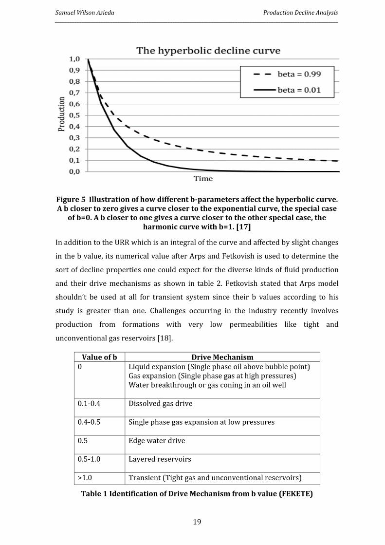
Figure 5 Illustration of how different b-parameters affect the hyperbolic curve. A b
closer to zero gives a curve closer to the exponential curve, the special case of b=0. A
b closer to one gives a curve closer to the other special case, the harmonic curve with
b=1. [16] ..................................................................................................................................................... 19
Figure 6 Production decline curve classifications [2] ............................................................. 21
Figure 7 A typical Fetkovich type curve [18] .............................................................................. 23
Figure 8 A typical Blasingame type curve [24] .......................................................................... 27
Figure 9 Material Balance Plot [18] ................................................................................................ 28
Figure 10 3D Reservoir Geometry .................................................................................................. 30
Figure 11 Reservoir Completion ...................................................................................................... 31
Figure 12 Oil PVT Data Plot ............................................................................................................... 32
Figure 13 Plot of Ln q(t) against t ................................................................................................... 36
Figure 14 Arps Model Forecast ........................................................................................................ 37
Figure 15 Production History Plot .................................................................................................. 38
Figure 16 Fetkovish Type Curve Plot ............................................................................................. 39
Figure 17 Blasingame Type Curve Plot ......................................................................................... 40
Figure 18 Normalized Rate-Cumulative Plot .............................................................................. 41
Figure 19 Sensitivity to Kh ................................................................................................................. 42
Figure 20 Sensitivity to Skin.............................................................................................................. 43

Samuel Wilson Asiedu Production Decline Analysis ______________________________________________________________________________________________________________________
vii
LIST OF TABLES
Table 1 Identification of Drive Mechanism from b value (FEKETE) ................................... 19
Table 2 ARPS’ EQUATIONS ................................................................................................................ 20
Table 3 Rock and Fluid Properties .................................................................................................. 31
Table 4 Parameters for Sensitivity ................................................................................................. 41
Table 5 Comparison of results from different methods .......................................................... 45

Samuel Wilson Asiedu Production Decline Analysis ______________________________________________________________________________________________________________________
1
1 Introduction
One widespread practice by petroleum engineers is to estimate hydrocarbon
reserves and to estimate or forecast the future performance of wells and also the
entire reservoir. This has so been achieved by many methods (Material Balance
Equation, Decline Curve and Type Curve technique), of which decline curve analysis
numbers among the earliest methods and yet the conventional tool most practically
applied. On a larger perspective, it aids as a means of identifying well production
problems. Its output (the estimation of remaining reserves) is completely dependent
and determined by certain initial conditions and the resolution of the history
production data of the well or field.
The entire production lifetime of hydrocarbon reservoirs shows three main phases
similar to what is described in figure 1: the ramp-up or build-up phase,
corresponding to the increasing field production rate as newly drilled and completed
producers are brought on stream; the plateau or peak phase, where a constant rate of
production is maintained which can last after some years for an oil field but longer
for a gas field; the rate decline phase, which is usually the longest period as all
producers would at this phase exhibit a decline in production [1]. For depletion drive
reservoirs, the peak phase is described by a decrease in bottomhole flowing pressure
until the decline phase where the flowing bottomhole pressure remains fairly
constant.
Figure 1 Idealized behavior of an oilfield production [1]
Samuel Wilson Asiedu Production Decline Analysis ______________________________________________________________________________________________________________________
2
Production data analysis is the most commonly used form of data analysis employed
in evaluation oil and gas production and predicting future performance. This data
analysis technique is grounded on the statement that the historical production trend
can be extrapolated and described by mathematical expressions. The method of
extrapolating a “trend” for the purpose of estimating future performance must gratify
the condition that the features which triggered changes in the past performance, i.e.,
decline in the flow rate, will function in the same way in the future [2]. The use of the
entire rate history from production to forecast the wells future performance is
achieved by the Arps empirical decline analysis. Though this method is extensively
applied and yields reliable results compared to other estimation methods, its results
can be compared to the others to evaluate new areas of investment. The projected
performance trend of the historical production is used in implementing technical
deductions, devising developmental strategies, making economic plans and as a
criterion to advice management.
Arps (1945) empirical method is applicable only to a stabilized reservoir (boundary
dominated flow) and assumes a constant bottomhole flowing pressure (BHFP). It
estimates the expected ultimate recovery (EUR) but cannot describe the transient
flow regime and determine the formation parameters unless extended by other
methods. Fetkovish (1980) began this extension by introducing the transient flow
equations in PTA to the Arps empirical equations making analysis possible for both
transient and boundary dominated flows and since its derived from the Arps
postulates, it also assumes a constant BHFP. Palacio and Blasingame (1993) removed
the limitation on the Arps and Fetkovish methods when they considered the
variability of the BHFP and the changes in Pressure-Volume-Temperature (PVT)
characteristics with pressure by normalizing the rate with the pressure changes and
introducing the concept of the material balance time (tc). They also used the flow rate
integral and its derivative as supplementary curves to reduce the uncertainty of
interpretation results [3].
1.1 Study Objectives
The core objective of this study is to provide an interpretation observed from a
history production data through the application of conventional, classical and
Samuel Wilson Asiedu Production Decline Analysis ______________________________________________________________________________________________________________________
3
modern production data analysis methods. Production data generated from a
synthetic reservoir model is used to envisage the future or the long-term production
performance of a well and to refine our understanding by identifying key parameters
that contributed to the production decline.
1.2 Scope of Work
This work involves a two-way approach; applying forward modelling by using a
numerical simulator to develop a synthetic reservoir model to create the production
data used in the analysis, and an inverse modelling approach by using an analytical
tool on the generated production data to describe the dynamic response from the
synthetic reservoir model. This analysis is based on a single producing well.
Production from multi wells draining the same reservoir are mostly manifolded,
hence a single well as in our case can be representative. As Decline curves still
remains a useful tool in production forecast, chapter 2 of this work is focused on
reviewing the various theoretical techniques applied and previous references related
to decline curves. In chapter 3, we applied the various techniques, the traditional
Arps method, classical Fetkovish’s type curves and the modern Blasingame’s type
curves, to our production data obtained from numerical simulation. Chapter 4
proceeds with the interpretation of our results and discussion to ascertain the
practical application of each technique with sensitivity analysis made on some
notable reservoir parameters and finally, work is concluded in chapter 5.
Samuel Wilson Asiedu Production Decline Analysis ______________________________________________________________________________________________________________________
4
2 Literature Review
This chapter lays a basis on which the proceeding chapters will be built on. In the
first subsection, the fundamentals of oil production are described and leads to
exposition of production decline in the next subsection. The techniques of decline
curve analysis (DCA) are discussed as well as the methods used for multiphase flows
and the impact resulting from drive mechanisms and reservoir rock and fluid
properties. The chapter completes with a description of theoretical work relating to
further developments to the DCA.
2.1 Basic Concept of Oil Production
The accumulation of conventional oil occurs through several geological processes of
organic materials buried over an extensive range of temperatures and pressures in
underground formations known as reservoirs. A typical reservoir is a rock of
considerable pore space where petroleum resides in the tiny void spaces between the
rock grains and is permeable as well, allowing for the rock to conduct the fluids
stored up within the pores, such as sandstone or carbonates. An oilfield may
comprise of one or numerous reservoirs in the subsurface accessible from the surface
by drilling. Distinction is usually made between unconventional and the conventional
oil resources; while the conventional resources are considered to be found in the
typical rock configurations with a source rock, a reservoir rock and a trap, the
unconventional resources are fossil resources where one or more of the components
of the conventional resources are missing.
Conventional oilfields account for more than 90 percent of global oil production, with
slight contributions coming from unconventional oil, natural gas liquids (ethane,
propane, butane and pentane) and other liquids [1]. Oil production fluid volume is
frequently measured in barrels (b or bbl) equivalent to a volume of 42 US gallons or
approximately 159 liters. Alternatively, production flow rate, expressed in barrels
per day (b/d or bbl/d) can be used. An oilfield may be described as a field containing
hydrocarbon, preferably oil, from less of a million barrels (MMbbl) to several billion
barrels (Bbbl). The overall number of oilfields number over 70,000 [4]. However, the
contribution of individual fields to the global oil supply varies widely, few hundreds
Samuel Wilson Asiedu Production Decline Analysis ______________________________________________________________________________________________________________________
5
of ‘giant’ fields (more than 500 million barrels) accounting for nearly one-half of total
oil production with about 25 fields accounting for one-fourth of it [1]. Thus, although
fields share parallel overall behavior, the degree of production can differ
significantly.
Höök [1] offers a typical production profile of an oilfield as seen in figure 1. His study
notes that, significant deviations can be triggered by development history, alteration
in production strategy or technology, oil price, political decisions, accidents, sabotage
and similar factors. For some fields, the plateau periods are very short, more like a
single peak, while others (especially large fields) may maintain relatively constant
production for many years. But, at some point in production time, all fields will reach
the inception of decline and as a result start to experience a decrease in production.
2.1.1 Oil Recovery Methods
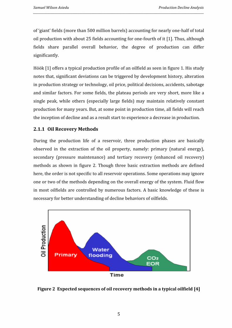
During the production life of a reservoir, three production phases are basically
observed in the extraction of the oil property, namely: primary (natural energy),
secondary (pressure maintenance) and tertiary recovery (enhanced oil recovery)
methods as shown in figure 2. Though three basic extraction methods are defined
here, the order is not specific to all reservoir operations. Some operations may ignore
one or two of the methods depending on the overall energy of the system. Fluid flow
in most oilfields are controlled by numerous factors. A basic knowledge of these is
necessary for better understanding of decline behaviors of oilfields.
Figure 2 Expected sequences of oil recovery methods in a typical oilfield [4]
Samuel Wilson Asiedu Production Decline Analysis ______________________________________________________________________________________________________________________
6
The physics of oil recovery is about flow of fluid through the porous media that
makes up the oilfield. Generally, movement of downhole fluids in a reservoir depend
on these outlined factors as described further expansively by Slatter et al (2008) [5]
• depletion (decline in reservoir flowing pressure),
• total compressibility of the system (rock or fluid or both),
• volume of gas phase dissolved into the liquid phase,
• angle of inclination (formation dip),
• capillary rise through minute pores,
• surrounding aquifer or overlying gas cap providing extra energy for pressure
maintenance
• water or gas injection, and
• manipulation of fluid properties or by thermal means.
2.1.1.1 Primary recovery
This is the first stage of petroleum production based on buoyancy (Archimedes
principle) and reservoir pressure, in which natural reservoir energy is used to push
the oil to the surface. During the initial phase of production, primary recovery
techniques are inherently applied by exploiting the natural energy within the
reservoir and using artificial lift procedures like pumps to push the oil to the surface.
In simple terms, the oil is made to flow under its own pressure, unless other fluids
are injected to sustain or support the energy of the reservoir system. This primary
recovery becomes limited at a point where the reservoir pressure is too low to
maintain economical production rates, that consequently results in a decline in the
rate of production. Typically, about 10-25% of the reservoirs oil originally in place is
extracted, making the proportion of the initial oil in place produced under the
primary recovery mechanism very small and therefore calls for extra methods to be
applied to ensure an optimum recovery [6].
2.1.1.2 Secondary recovery
The concentration of secondary recovery is on artificial pressure maintenance (APM)
strategy, where fluids are carefully injected to support the energy of the system by
maintaining reservoir pressure. In significantly larger oilfields, the largest percentage
Samuel Wilson Asiedu Production Decline Analysis ______________________________________________________________________________________________________________________
7
of the total oil recovery is achieved by secondary recovery methods [7]. One of the
mostly applied secondary recovery method for maintaining the reservoir pressure is
water flooding, done by injecting water in an area just beneath the oil-water contact.
When success of this method is achieved, the water forms a bank and pushes the oil
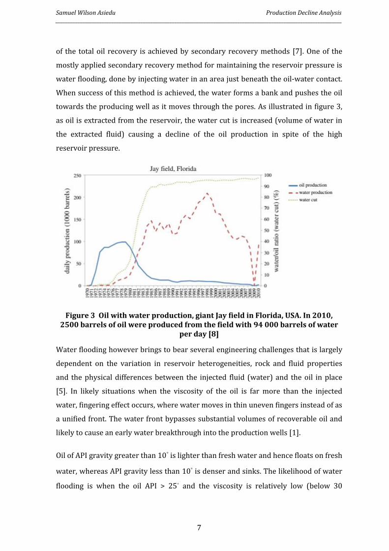
towards the producing well as it moves through the pores. As illustrated in figure 3,
as oil is extracted from the reservoir, the water cut is increased (volume of water in
the extracted fluid) causing a decline of the oil production in spite of the high
reservoir pressure.
Figure 3 Oil with water production, giant Jay field in Florida, USA. In 2010, 2500 barrels of oil were produced from the field with 94 000 barrels of water
per day [8]
Water flooding however brings to bear several engineering challenges that is largely
dependent on the variation in reservoir heterogeneities, rock and fluid properties
and the physical differences between the injected fluid (water) and the oil in place
[5]. In likely situations when the viscosity of the oil is far more than the injected
water, fingering effect occurs, where water moves in thin uneven fingers instead of as
a unified front. The water front bypasses substantial volumes of recoverable oil and
likely to cause an early water breakthrough into the production wells [1].
Oil of API gravity greater than 10◦ is lighter than fresh water and hence floats on fresh
water, whereas API gravity less than 10◦ is denser and sinks. The likelihood of water
flooding is when the oil API > 25◦ and the viscosity is relatively low (below 30
Samuel Wilson Asiedu Production Decline Analysis ______________________________________________________________________________________________________________________
8
centipoise). It works best in homogeneous reservoir formations. Consequently, as the
majority of the world’s oil producing fields attempts the secondary recovery, it’s not
always effective. A combination of primary and secondary recovery methods can
extract to about 30–50% of the oil in place and nearly most reservoirs that can take
advantage from APM are making use of it [1, 5].
2.1.1.3 Tertiary (enhanced) oil recovery
Enhanced Oil Recovery (EOR) methods which has become a more recognized term in
petroleum engineering literature instead of the usual tertiary recovery involves more
compound ways of manipulating rock and fluid properties targeted at increasing the
mobility of the oil to increase production [9].
According to Darcy’s law, oil movement can be enhanced in a reservoir by decreasing
its viscosity as long as delta pressure remains constant. For this reason, four key
methods to EOR has been presented by Höök et al (2014), that is chemical, thermal,
miscible and microbial methods; which are presented below.
The most commonly used approach is the thermal method which makes up to almost
half of entire worldwide EOR projects. Thermal EOR method, as the name implies,
comprises of altering the viscosity of oil by thermal means, such as hot-water
flooding, steam flooding or in situ combustion, which produces heat that burns a
portion of the oil in place by igniting the bottommost reservoir formation.
Miscible methods focus on injection of a gas or solvent miscible with the oil resulting
in an improved recovery efficiency. It accounts for near 41% of worldwide EOR
projects. Though the miscibility enhances the mobility of the oil, it also significantly
adds up to the intricacies of the process. Carbon dioxide injection is widely applicable
to many reservoirs than other methods at lower miscibility pressures [1, 5]. What
actually happens is that, the net volume swells up as a portion of the CO2 dissolves in
the oil and reduces the viscosity of the oil. Due to the low interfacial tension, it makes
it possible for the CO2 and oil to flow together as the miscibility progresses. Lighter
hydrocarbons (mainly natural gas) if available, can as well be injected to create
miscibility which decreases the oil viscosity while increasing oil volume via same
swelling process. In high-permeability reservoir formations holding light oil, nitrogen
or flue gas, is sometimes a substitute. From an oil recovery standpoint, these gases
Samuel Wilson Asiedu Production Decline Analysis ______________________________________________________________________________________________________________________
9
are generally somewhat less expensive, but inferior to CO2 or the lighter
hydrocarbons [1, 5].
Chemical flooding applies the injection of polymers, surfactants, and caustic alkaline
or other chemicals. Presently, on the global perspective, chemical flooding makes up
to about 11% of EOR projects. The conditions favorable for the water flooding
technique is also applied here since they are grounded on similar principle save the
polymer used instead of water. Polymers can be used to enhance water flooding
process by changing water viscosity and mobility. After the water floods, more oil
will be produced in the initial stage, and this is the key economic benefit, as ultimate
recovery is mostly the same as for conventional water flooding [1, 5]. Surfactants are
also used to recover extra oil by enhancing mobility and solubility of oil and
emulsifying oil and water.
2.2 Fundamentals of fluid flow
The transport of petroleum fluid through the reservoir formation is to a significant
extent dictated by physical properties related to the geological formation of the
reservoir under discussion and the characteristics of the petroleum it contains.
Disparities in these characteristics cause production rates to vary from field to field.
A reservoir houses its fluid in tiny microscopic pores inside the rock formation, and
the term porosity of a rock is defined as the ratio of the pore spaces to the rocks bulk
volume. The larger the porosity, the better the rock is at storing fluids.
In 1856 a French physicist, Henry Darcy, investigated the flow of fluid through a
layered bed of packed sand and came up with an expression to describe the fluids’
behavior, which is now known to be Darcy’s law (equation 2.1). The equation
postulated by Darcy considers important physical properties such as its permeability
which is the capacity of the porous media to conduct the fluid and its viscosity which
describes the degree of internal resistance to fluid flow. Comparing viscous forces to
gravity and capillary forces, the influence of the viscosity to fluid flow both produced
and injected fluids under normal conditions are superior than the later forces. This
suggests that fluids flowing through parallel layered porous media encounters few
disruptions (i.e. laminar flow conditions) and the rate of fluid flow is directly
relational to the pressure gradient in the reservoir [5].
Samuel Wilson Asiedu Production Decline Analysis ______________________________________________________________________________________________________________________
10
q = −kA
μ ∂P
∂L (2.1)
where q is the volumetric flow rate (cm3/s), k is the permeability (darcy), A is the
cross-sectional area to the flow (cm2), µ is the viscosity (centipoise), and 𝜕𝑃⁄𝜕𝐿 is the
pressure gradient over the length of the fluid flow path (atm/cm)2
Equation 2.1 describes a unidirectional flow, where the fluid is transmitted straight
in one single direction. However, the flow inside the rock formation is far more
complicated. Despite this, Darcy’s law is important when studying fluid flow in oil
reservoirs since it gives the physical boundaries to the possible production rate and
indicates in what manner the flow rate is affected by the different parameters [10].
The negative sign shows that the fluid flows from high pressure to low pressure. The
key constraint for the fluid to flow is the pressure gradient hence the greater the
pressure gradient, the greater the flow rate. When recovering oil or gas from a
reservoir, the pressure gradient decreases along with the extraction. When the
pressure in the reservoir has decreased to a level too low to drive the flow any longer
the pressure can be maintained by feeding additional energy into the reservoir by a
secondary recovery method, injecting water and/or gas [11].
Basically, Darcy’s law states that a fluid which has a high viscosity will have a low
flow rate at constant delta pressure; and that if the rock permeability is high, a high
flow rate is anticipated; and that pressure gradient is necessary for fluid to flow. The
negative sign in the Darcy’s equation also indicates that the fluid flows oppositely
(from higher to lower potential) of the pressure gradient [1].
2.3 Production Decline and Decline Rate
Oil and gas wells usually reach their peak output shortly after completion shown in
figure 1, and from that time begins to decline. Wells completed in water-drive
reservoirs may not suffer an early decline due to the support from the aquifer. The
speed of decline depends on the output of the wells and on other factors as earlier
described.
When estimating future production in an oil field or an oil well, the idea of decline
rate is fundamental. The decline rate, λ, is the reduction in the production rate from
an individual well, or a group of wells, after the production has peaked and is

Samuel Wilson Asiedu Production Decline Analysis ______________________________________________________________________________________________________________________
11
regularly stated on an annual or monthly or sometimes daily basis. Changes can
either be positive or negative but are usually negative so long as a field has passed its
peak of production [1]. It is expressed below;
Decline raten =Productionn−Productionn−1
Productionn−1 (2.2)
Physical and intrinsic factors driving the oil depletion like falling reservoir pressure,
increasing water cut etc., does not certainly relate to the decline rate studies. Non-
physical factors such as underinvestment, government policies, production shares,
damage or interruption has been observed to affect decline. In essence, decline rates
simply provide uncertain indications for unguarded analysts. Compound connections
between reservoir physics, economics, technology and decision-making has been
found to frequently influence decline in production. Production rates are influenced
by many factors and much care must be taken in extrapolating decline trend into the
future [1]. Decline rates seen in actual oilfields can vary significantly and research
has shown that those of small fields may vary from those of giant fields [11].
Since the early years of the petroleum industry, increasing exploitation and depleting
reserves have been related to declining production. The analysis of decline curves
has since then been a practical tool for predicting field behavior and forecasting well
life.
2.4 Comparing Predictive Models
Several models have so far been developed to estimate the original hydrocarbon in
place with the knowledge of some existing data acquired either through well log
interpretation, experimental analysis or pressure transient tests. These models use
numerical computations to arrive at their results.
The results of these computations can be presented as 1-, 2-, or 3-dimensional spatial
analysis of the reservoir operating under diverse well-configuration and different
conditions of depletion. These studies take a lot of time and is costly as well and
therefore calls for more information than required for a study of the decline curve
characteristics [12].
Samuel Wilson Asiedu Production Decline Analysis ______________________________________________________________________________________________________________________
12
Reservoir evaluation and the science of projecting future production can be sectioned
into four areas that roughly correspond to the allotted time and effort to be
consumed as well as the quantity and quality of information [12]. The advantages and
flaws of each method is herein discussed as described by Poston (2007);
2.4.1 Volumetric Method
The volume of hydrocarbon (N or G for oil and gas respectively) in the subsurface
reservoir formation depends on the reservoir bulk volume (Vb), fraction of the bulk
volume which is porous (∅), and the connate water saturation (Swc). The equations
below apply to oil and gas respectively;
N =Vb∅(1−Swc)
Boi (2.3)
G =Vb∅(1−Swc)
Bgi (2.4)
The volumetric method is an easy to understand evaluation technique for defining
hydrocarbon in-place. It’s a low-cost method such that isopach maps can be
combined with structural maps to provide a comprehensive picture for making
reservoir and field extent estimations. This method however has several limitations;
the results are dependent on the well spacing and the quality of porosity and
saturation values which are mostly not achieved due to the degree of reservoir
heterogeneities, especially using a single porosity as a representative for the entire
reservoir formation; the maps are also unable to generate future forecast and
difficulty in predicting recovery from layered or naturally fractured formation or in
reservoirs with commingled production [12].
2.4.2 Decline Curves Method
Many years ago, discovery has shown that plotting rate of production against time for
a single or several wells can be inferred into the future to provide an approximation
of the future rates of production of a well. With the future rates known, it is of course
possible to determine the future total production or reserves of the well [13].
Samuel Wilson Asiedu Production Decline Analysis ______________________________________________________________________________________________________________________
13
It’s of a great advantage to apply production decline curves due to the readily
availability of production data. It’s a low-cost method and time efficient as well as
being easy to be programmed for operation on personal computers [12].
The analysis of production decline curves comes with its own limitations some of
which include; the alteration of the profile of the decline curve when operating
conditions are changed, inability to quantitatively infer the reservoir characteristics
from the shape of the curve, and the struggle in interpretation of the future
performance in low-permeability, multilayered or fractured reservoirs due to the
high variability and uncertain effects of crossflow. Changes in operating conditions or
any probable changes must be carefully considered when developing the equation
representing a production decline curve and, more particularly, when predicting
performance. [12].
2.4.3 Material Balance Method
Reserve estimation with material balance (Shilthuis Equation) is based on production
history data. Pressure-dependent rock and fluid properties are built into a reservoir
material-balance-type equation. The material-balance analysis is a tank-type model
based on the conservation of mass, which does not take into consideration variable
flow conditions.
For a saturated oil reservoir with constant porous volume, its material balance on a
cartesian plot produces a straight line with a slope of slope N (Oil Originally in Place)
as shown in the equation below;
Np[Bo + Bg(Rp − Rs)] = N[Bo − Boi + Bg(Rsi − Rs)] (2.5)
The strong point of material-balance-type calculations include; Pressure-dependent
reservoir rock and fluid properties, as well as the production history are included in a
reservoir model; it is also a low-cost and time efficient analysis method that can be
easily computed with a computer program. This method can also be easily applied to
determine the depletion efficiency in a moderate-to-high permeability field.
Recovery factor is needed to calculate reserves which makes the material balance
method a weak asset in such estimation. Moreover, vertical and areal variations in
the reservoir character must be included as part of the reserves calculations.
Samuel Wilson Asiedu Production Decline Analysis ______________________________________________________________________________________________________________________
14
Recovery factors should be applied only to fairly homogeneous, modest-sized
reservoirs in which the producing zone exhibits permeability greater than 100 md
for oil reservoirs and 1 md or less for gas reservoirs [12].
2.4.4 Reservoir Simulation Method
The reservoir is upscaled and divided into a grid system. It applies a combination of
several equations; material balance equation, diffusivity flow equation, and equation
of state into an iterative process to calculate the effect of the depletion history for
each cell in the system.
They can be applied to a 2D or 3D system and also to systems with widely changing
fluid composition; it allows all probable variables to be involved in the model making
it easy to study the effects of reservoir heterogeneity and variation on future
performance.
The reservoir simulation method generally requires a person skilled in the technique
of running the model to be involved in the study; the models comes with its
complications and requires a considerable amount of time, effort and expense to run
and a huge volume of field data. The field model is often simplified by forcing
reservoir heterogeneities and geology to fit the computer model, therefore, the
results obtain are dependent on the quality of the input data [12].
2.5 The Decline Curve Analysis
Firstly, presented by Arps [14], decline curve analysis’ is a tool used extensively to
model and forecast production under the basic assumption that the driving
mechanism controlling the decline is depletion drive thus water drive is not in
existence. The used analysis techniques assume that the historical production trend
will stay same in the future, and hence could be expressed mathematically and the
productive indexes of the producing wells remains constant such that the reservoir
production rate is proportional to the change in reservoir pressure. The methodology
comprises analyzing production history and fitting certain type curves to the flowing
production data. The future production behavior can be predicted by extrapolating
the type curves. The great advantage of the methodology is that little data is required.
Only production data of sufficient length to cover the behavior is needed. A weak side
Samuel Wilson Asiedu Production Decline Analysis ______________________________________________________________________________________________________________________
15
is that non-physical factors such as government policies and production shares may
also be reflected by the production data hence care needs to be taken when
extrapolating production trends into the future.
Three factors characterize decline curves; initial rate of production (production at a
certain time), shape of the decline trend and rate at which the production declines.
The decline rate (see equation 2.2), λ, can also be expressed by means of derivatives
where q is production rate and t is time in arbitrary units. The solution in the
differential equation form allows for the expression of decline characteristics using
the decline rate (λt), its exponent (b) and a constant denoted C [1]
λt = −q̇
q= −
dqdt
⁄
q= Cqb (2.6)
The expression in equation 2.6 implies that the decline can be constant (b = 0),
directly proportional to production rate (b = 1) or proportionate to the fractional
power of the production rate (0 < b < 1). The presence of the negative sign in the
expression is a way of converting the negative decline rate to a positive one [12]. This
simple expression explains why no detailed reservoir data like permeability and
saturations are required for the decline curve extrapolations, but van be simply done
with the available production data which is somewhat acquired easily. The curve-
fitting method can also be used to evaluate ultimate recovery of the field. Several
reservoir studies of oil depletion have shown that, cases that involves the sum of
production from individual fields are mostly achieved with decline curve forecasts
and also for analyzing a single field or well [1]. Since its introduction by Arps, several
different decline curve models have been developed, all of which are hinged to the
work developed by Arps [14].
2.5.1 Arps Decline Curve Analysis
Arps (1945) proposed that the curve of the production rate against time can be
expressed by one of the hyperbolic family equations; Exponential (constant
percentage) decline, Harmonic decline and Hyperbolic decline. Mathematically, his
proposal was based on the theoretical concept of loss-ratio (1/D) and the derivative
of the loss-ratio (b), where D and b are the decline curve parameter and decline curve
exponent, respectively, expressed as follows [14]
Samuel Wilson Asiedu Production Decline Analysis ______________________________________________________________________________________________________________________
16
1
D= −
q
dqdt
⁄=
1
λt (2.7)
D = −1
q
dq
dt (2.8)
b =d
dt(
1
D) = −
d
dt(
q
dqdt
⁄) (2.9)
where 0 ≤ b ≤ 1
qt =qi
(1+bDit)1b
(3.0)
Np =qi−q
D (3.1)
where
qt = production flow rate at time t, stb/day or stb/time
qi = initial flow rate, stb/day or stb/time
Di = initial decline rate constant, 1/day or 1/time
Np = Cumulative production at time t, STB
b = Arp’s decline curve exponent.
t = time
The above equations are strictly applicable for pseudo-steady state flow conditions
(the existence of a boundary-dominated flow regime) which is observed for most
conventional reservoirs. The assumption governing Arp’s analysis rate-time decline
curves are constant drainage areas, wells are producing at or near capacity and
operation is under constant bottom-hole pressure. The idealistic shape of each of the
hyperbolic family equations from Arps’s deduction is shown in figure 4.
Samuel Wilson Asiedu Production Decline Analysis ______________________________________________________________________________________________________________________
17
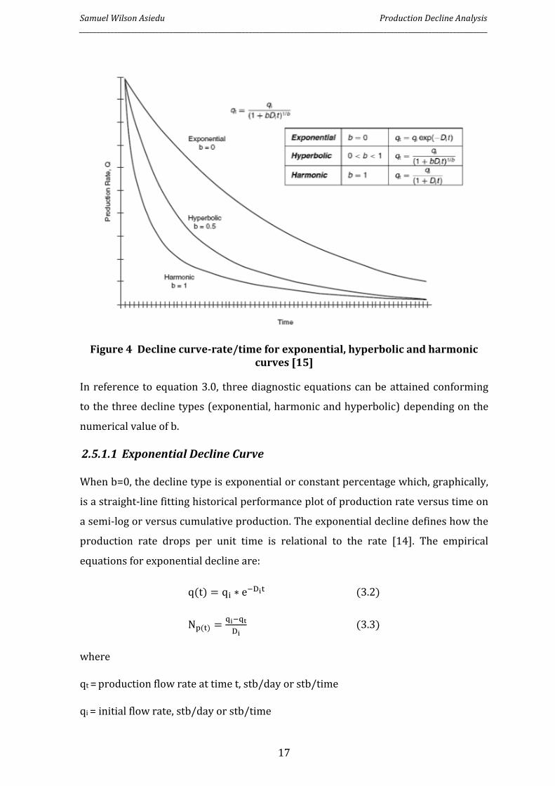
Figure 4 Decline curve-rate/time for exponential, hyperbolic and harmonic curves [15]
In reference to equation 3.0, three diagnostic equations can be attained conforming
to the three decline types (exponential, harmonic and hyperbolic) depending on the
numerical value of b.
2.5.1.1 Exponential Decline Curve
When b=0, the decline type is exponential or constant percentage which, graphically,
is a straight-line fitting historical performance plot of production rate versus time on
a semi-log or versus cumulative production. The exponential decline defines how the
production rate drops per unit time is relational to the rate [14]. The empirical
equations for exponential decline are:
q(t) = qi ∗ e−Dit (3.2)
Np(t) =qi−qt
Di (3.3)
where
qt = production flow rate at time t, stb/day or stb/time
qi = initial flow rate, stb/day or stb/time
Samuel Wilson Asiedu Production Decline Analysis ______________________________________________________________________________________________________________________
18
Di = initial decline constant
Np = Cumulative production at time t, STB
2.5.1.2 Hyperbolic Decline Curve
Hyperbolic decline is for the limit 0 < b < 1. The hyperbolic decline plot is a curve
(concave upwards) on the semi-log rate-time, since decline exponents change with
time, in contrast to the constant percentage decline [16]. Typical low productivity
wells exhibit hyperbolic-harmonic decline behavior [16]. Arps’ hyperbolic modeling
equations are as follows:
qt =qi
(1+bDit)1b
(3.4)
Np(t) =qi
Di(1−b)[1 − (
qt
qi)
(1−b)
] (3.5)
where
qt = production flow rate at time t, stb/day or stb/time
qi = initial flow rate, stb/day or stb/time
Di = initial decline rate constant, 1/day or 1/time
Np(t) = Cumulative production at time t, STB
b = Arp’s decline curve exponent.
t = time
The influence of the b value on the hyperbolic curve ranging 0.01 to 0.99 was
investigated by Hooke et al (2014) and illustrated in figure 5. In reservoir studies, the
Ultimate Recoverable Reserves (URR) is considered to be the integral of the curve.
Hence, only slight changes in the b-parameter have large impacts on the URR [1]. The
higher the b-parameter, the greater the URR estimate. The hyperbolic decline curve
suffers the danger of overestimating the URR and subsequently the economic yield of
a project, creating an argument to abandon the hyperbolic curve for a less optimistic
project concerning the late production (“tail production”) [1]
Samuel Wilson Asiedu Production Decline Analysis ______________________________________________________________________________________________________________________
19
Figure 5 Illustration of how different b-parameters affect the hyperbolic curve. A b closer to zero gives a curve closer to the exponential curve, the special case
of b=0. A b closer to one gives a curve closer to the other special case, the harmonic curve with b=1. [17]
In addition to the URR which is an integral of the curve and affected by slight changes
in the b value, its numerical value after Arps and Fetkovish is used to determine the
sort of decline properties one could expect for the diverse kinds of fluid production
and their drive mechanisms as shown in table 2. Fetkovish stated that Arps model
shouldn’t be used at all for transient system since their b values according to his
study is greater than one. Challenges occurring in the industry recently involves
production from formations with very low permeabilities like tight and
unconventional gas reservoirs [18].
Value of b Drive Mechanism 0 Liquid expansion (Single phase oil above bubble point)
Gas expansion (Single phase gas at high pressures) Water breakthrough or gas coning in an oil well
0.1-0.4 Dissolved gas drive
0.4-0.5 Single phase gas expansion at low pressures
0.5 Edge water drive
0.5-1.0 Layered reservoirs
>1.0 Transient (Tight gas and unconventional reservoirs)
Table 1 Identification of Drive Mechanism from b value (FEKETE)

Samuel Wilson Asiedu Production Decline Analysis ______________________________________________________________________________________________________________________
20
2.5.1.3 Harmonic Decline Curve
When b=1, decline is harmonic and forms a straight line on the semi-log plot of
production rate versus cumulative production. The empirical equations for harmonic
decline are:
qt =qi
(1+Dit) (3.6)
Np(t) = qi
Diln [(
qi
qt)] (3.7)
where
qt = production flow rate at time t, stb/day or stb/time
qi = initial flow rate, stb/day or stb/time
Di = initial decline rate constant, 1/day or 1/time
Np(t) = Cumulative production at time t, STB
b = Arp’s decline curve exponent.
t = time
On a linear plot of production vs time (see figure 5), the harmonic model gives a
decline curve that approaches an asymptote of a constant rate of production greater
than zero in the long run. In other words, the harmonic curve ends up in an infinite
URR, which cannot be probable in reality.
Table 1 is a summary of the variants of Arp’s production decline curve equations
Table 2 ARPS’ EQUATIONS
EXPONENTIAL HYPERBOLIC HARMONIC
DECLINE RATE qi − qt
(Np) (
qi
qt)
b
− 1
bt
= {qi
Np(1 − b)} {1
− [(qi
qt
)1−b
]}
qi
qt− 1
(t)=
qi
Np
lnqi
qt
Samuel Wilson Asiedu Production Decline Analysis ______________________________________________________________________________________________________________________
21
PROD. RATE, q qt = qi ∗ e−Dit qt =qi
(1 + bDit)1b
qt =qi
(1 + Dit)
CUM.PROD.,Np(t) Np(t) =qi − qt
Di
Np(t) =qi
Di(1 − b)[1 − (
qt
qi
)(1−b)
] Np(t) = qi
Diln [(
qi
qt)]
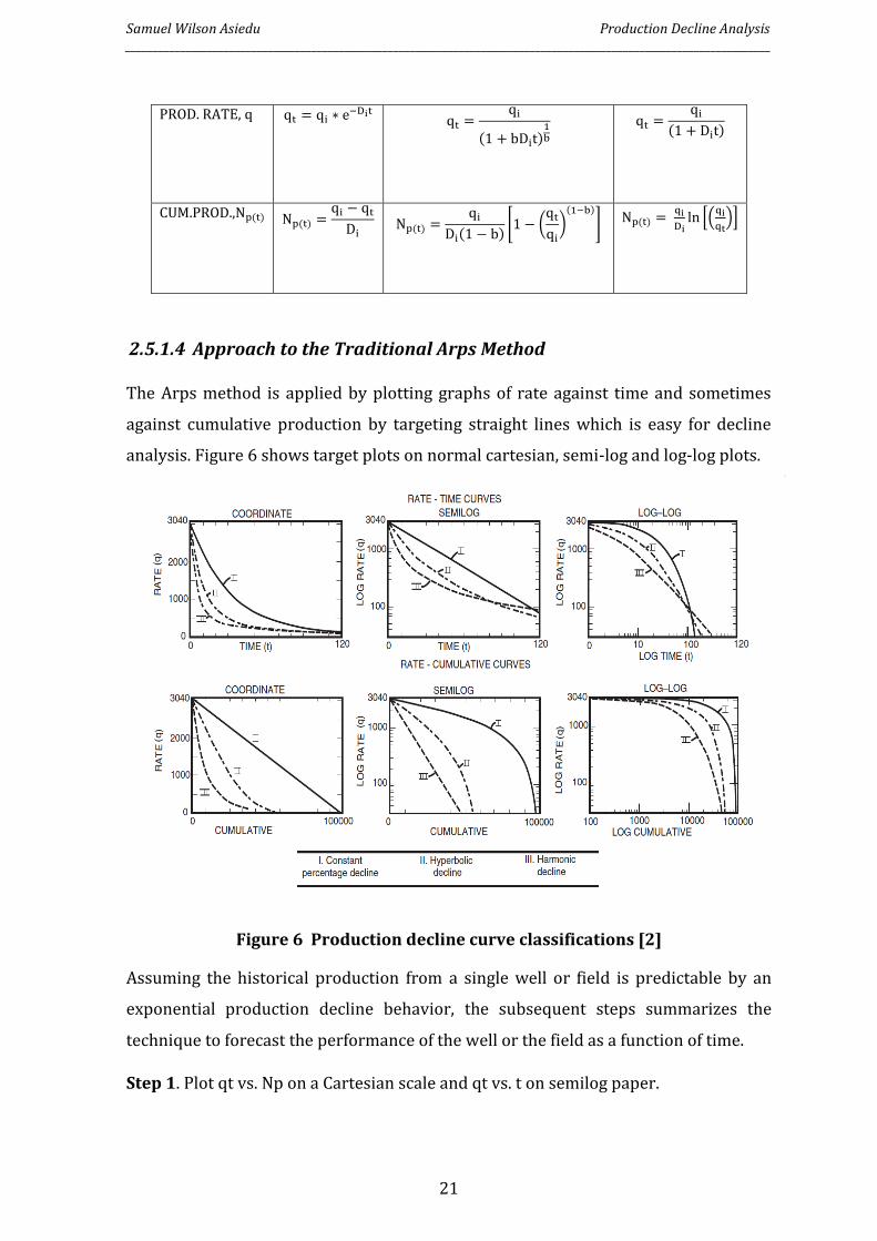
2.5.1.4 Approach to the Traditional Arps Method
The Arps method is applied by plotting graphs of rate against time and sometimes
against cumulative production by targeting straight lines which is easy for decline
analysis. Figure 6 shows target plots on normal cartesian, semi-log and log-log plots.
Figure 6 Production decline curve classifications [2]
Assuming the historical production from a single well or field is predictable by an
exponential production decline behavior, the subsequent steps summarizes the
technique to forecast the performance of the well or the field as a function of time.
Step 1. Plot qt vs. Np on a Cartesian scale and qt vs. t on semilog paper.

Samuel Wilson Asiedu Production Decline Analysis ______________________________________________________________________________________________________________________
22
Step 2. For both plots, draw the line of best fit through the points.
Step 3. Extrapolate the straight line on qt vs. Np to Np = 0 which intercepts the qt
axis at a flow rate value identified as the initial flow rate, qi.
Step 4. The initial decline rate, Di, is calculated by picking a point on the straight line
with coordinates of (qt, Np) or on a semilog line with coordinates of (qt, t) and
applying the exponential equations.
Step 5. Estimate the time to reach the economic flow rate limit qa (or any rate) and
the equivalent cumulative production from the exponential Equations in table 1. [2]
2.6 Further Developments to the Decline Curve Analysis (DCA)
Otherwise known as production analysis or rate transient analysis, various decline
curve analysis techniques for production forecasting have been established by
several authors for dealing with specific reservoir problems. Most of these methods
and techniques were improvements on the Arps traditional equations.
Pressure Transient Analysis is achieved with the availability of pressure and rate
data but has recently been complimented with the development of Production
Analysis (PA). Both analysis is achieved with the spread of Permanent Downhole
Gauge (PDG), which extract data applicable for both analysis techniques [19] .
The Arps decline curves are not applicable to all reservoirs due to its empirical
nature but applied as deemed fitting for any specific scenario. Some advanced models
of the decline curves for specific reservoir conditions are outlined below;
2.6.1 Fetkovish DCA
Fetkovich came up with his findings after identifying that the conventional Arps
decline method was applicable only during the depletion period (boundary
dominated flow condition) and for that matter, did not account for the early
production life (transient flow period) of the well. Fetkovich used analytical flow
equations in dimensionless terms to develop type curves which incorporated the
empirical decline curve equations initially documented by J.J. Arps resulting in its use
to analyze both transient and boundary-dominated flows [20].
Samuel Wilson Asiedu Production Decline Analysis ______________________________________________________________________________________________________________________
23
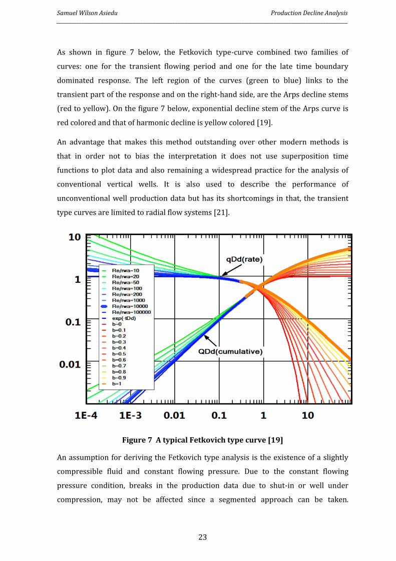
As shown in figure 7 below, the Fetkovich type-curve combined two families of
curves: one for the transient flowing period and one for the late time boundary
dominated response. The left region of the curves (green to blue) links to the
transient part of the response and on the right-hand side, are the Arps decline stems
(red to yellow). On the figure 7 below, exponential decline stem of the Arps curve is
red colored and that of harmonic decline is yellow colored [19].
An advantage that makes this method outstanding over other modern methods is
that in order not to bias the interpretation it does not use superposition time
functions to plot data and also remaining a widespread practice for the analysis of
conventional vertical wells. It is also used to describe the performance of
unconventional well production data but has its shortcomings in that, the transient
type curves are limited to radial flow systems [21].
Figure 7 A typical Fetkovich type curve [19]
An assumption for deriving the Fetkovich type analysis is the existence of a slightly
compressible fluid and constant flowing pressure. Due to the constant flowing
pressure condition, breaks in the production data due to shut-in or well under
compression, may not be affected since a segmented approach can be taken.
Samuel Wilson Asiedu Production Decline Analysis ______________________________________________________________________________________________________________________
24
However, Fetkovish analysis will not work for a rate restricted production [18]. The
original type-curve presented by Fetkovich displayed rate only but to reduce the
effect of the noise and bring more confidence in the matching process a merged
presentation including the cumulative was later introduced similar to figure 7 [19].
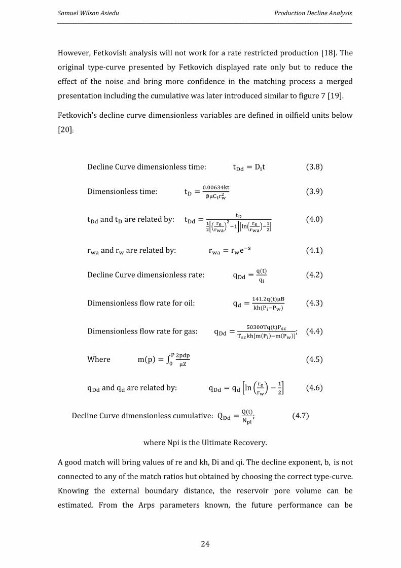
Fetkovich’s decline curve dimensionless variables are defined in oilfield units below
[20];
Decline Curve dimensionless time: tDd = Dit (3.8)
Dimensionless time: tD =0.00634kt
∅μCtrw2 (3.9)
tDd and tD are related by: tDd =tD
1
2[(
rerwa
)2
−1][ln(re
rwa)−
1
2] (4.0)
rwa and rw are related by: rwa = rwe−s (4.1)
Decline Curve dimensionless rate: qDd =q(t)
qi (4.2)
Dimensionless flow rate for oil: qd =141.2q(t)μB
kh(Pi−Pw) (4.3)
Dimensionless flow rate for gas: qDd =50300Tq(t)Psc
Tsckh[m(Pi)−m(Pw)]; (4.4)
Where m(p) = ∫2pdp
μZ
P
0 (4.5)
qDd and qd are related by: qDd = qd [ln (re
rw) −
1
2] (4.6)
Decline Curve dimensionless cumulative: QDd =Q(t)
Npi; (4.7)
where Npi is the Ultimate Recovery.
A good match will bring values of re and kh, Di and qi. The decline exponent, b, is not
connected to any of the match ratios but obtained by choosing the correct type-curve.
Knowing the external boundary distance, the reservoir pore volume can be
estimated. From the Arps parameters known, the future performance can be
Samuel Wilson Asiedu Production Decline Analysis ______________________________________________________________________________________________________________________
25
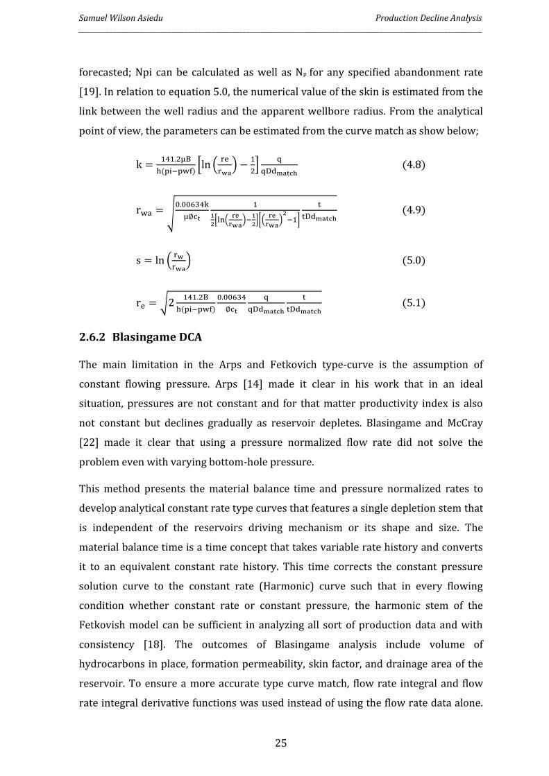
forecasted; Npi can be calculated as well as Np for any specified abandonment rate
[19]. In relation to equation 5.0, the numerical value of the skin is estimated from the
link between the well radius and the apparent wellbore radius. From the analytical
point of view, the parameters can be estimated from the curve match as show below;
k =141.2μB
h(pi−pwf)[ln (
re
rwa) −
1
2]
q
qDdmatch (4.8)
rwa = √0.00634k
μ∅ct
1
1
2[ln(
re
rwa)−
1
2][(
re
rwa)
2−1]
t
tDdmatch (4.9)
s = ln (rw
rwa) (5.0)
re = √2141.2B
h(pi−pwf)
0.00634
∅ct
q
qDdmatch
t
tDdmatch (5.1)
2.6.2 Blasingame DCA
The main limitation in the Arps and Fetkovich type-curve is the assumption of
constant flowing pressure. Arps [14] made it clear in his work that in an ideal
situation, pressures are not constant and for that matter productivity index is also
not constant but declines gradually as reservoir depletes. Blasingame and McCray
[22] made it clear that using a pressure normalized flow rate did not solve the
problem even with varying bottom-hole pressure.
This method presents the material balance time and pressure normalized rates to
develop analytical constant rate type curves that features a single depletion stem that
is independent of the reservoirs driving mechanism or its shape and size. The
material balance time is a time concept that takes variable rate history and converts
it to an equivalent constant rate history. This time corrects the constant pressure
solution curve to the constant rate (Harmonic) curve such that in every flowing
condition whether constant rate or constant pressure, the harmonic stem of the
Fetkovish model can be sufficient in analyzing all sort of production data and with
consistency [18]. The outcomes of Blasingame analysis include volume of
hydrocarbons in place, formation permeability, skin factor, and drainage area of the
reservoir. To ensure a more accurate type curve match, flow rate integral and flow
rate integral derivative functions was used instead of using the flow rate data alone.
Samuel Wilson Asiedu Production Decline Analysis ______________________________________________________________________________________________________________________
26
These integral functions are also capable of removing problems associated with
production data with inconsistent rate and bottom-hole pressure behavior. Different
reservoir types make a practical use of the Blasingame type curve method and
include:
• Radial and Elliptical flow wells
• Wells produced under water drive mechanism
• Fractured wells (cylindrical)
• Horizontal well
With this method, given a type curve match, formation permeability, skin, fracture
half length, dimensionless fracture conductivity, drainage area, original oil- or gas-in-
place can be found if reservoir thickness, total compressibility, and wellbore radius
are known [20].
Palacio and Blasingame [23] further came up with type-curves that could be used
extensively for variable flowing pressure conditions. The Bourdet [24] derivative was
also considered to offer improvement to the type-curve analysis, but due to the noise
characteristic of the production data, the derivative was applied to the normalized
flow rate integral but not to the normalized flow rate. More precisely, the Palacio-
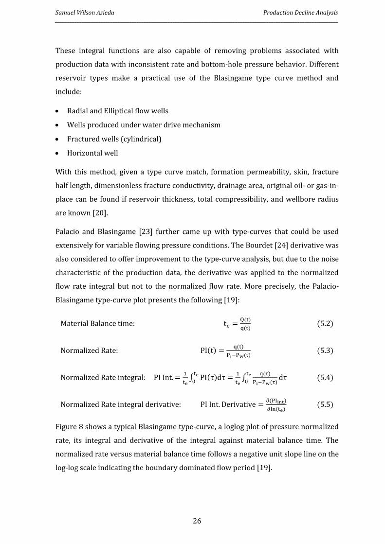
Blasingame type-curve plot presents the following [19]:
Material Balance time: te =Q(t)
q(t) (5.2)
Normalized Rate: PI(t) =q(t)
Pi−Pw(t) (5.3)
Normalized Rate integral: PI Int. =1
te∫ PI(τ)dτ
te
0=
1
te∫
q(τ)
Pi−Pw(τ)dτ
te
0 (5.4)
Normalized Rate integral derivative: PI Int. Derivative =∂(PIint)
∂ln (te) (5.5)
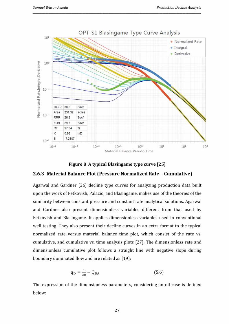
Figure 8 shows a typical Blasingame type-curve, a loglog plot of pressure normalized
rate, its integral and derivative of the integral against material balance time. The
normalized rate versus material balance time follows a negative unit slope line on the
log-log scale indicating the boundary dominated flow period [19].
Samuel Wilson Asiedu Production Decline Analysis ______________________________________________________________________________________________________________________
27
Figure 8 A typical Blasingame type curve [25]
2.6.3 Material Balance Plot (Pressure Normalized Rate – Cumulative)
Agarwal and Gardner [26] decline type curves for analyzing production data built
upon the work of Fetkovish, Palacio, and Blasingame, makes use of the theories of the
similarity between constant pressure and constant rate analytical solutions. Agarwal
and Gardner also present dimensionless variables different from that used by
Fetkovish and Blasingame. It applies dimensionless variables used in conventional
well testing. They also present their decline curves in an extra format to the typical
normalized rate versus material balance time plot, which consist of the rate vs.
cumulative, and cumulative vs. time analysis plots [27]. The dimensionless rate and
dimensionless cumulative plot follows a straight line with negative slope during
boundary dominated flow and are related as [19];
qD =1
2π− QDA (5.6)
The expression of the dimensionless parameters, considering an oil case is defined
below:
Samuel Wilson Asiedu Production Decline Analysis ______________________________________________________________________________________________________________________
28
qd =141.2qμB
kh(Pi−Pw) (5.7)
QDA =0.8936QB
∅hACt(Pi−Pw) (5.8)
The dimensionless cumulative production can as well be stated in terms of the fluid
in place, in STB/D:
N =∅hA
5.615B (5.9)
QDA =0.8936QB
∅hACt(Pi−Pw)=
Q
2πNCt(Pi−Pw) (6.0)
So, the linear relationship between dimensionless rate and cumulative becomes:
141.2qμB
kh(Pi−Pw)=
1
2π−
0.8936QB
5.615NCt(Pi−Pw) (6.1)
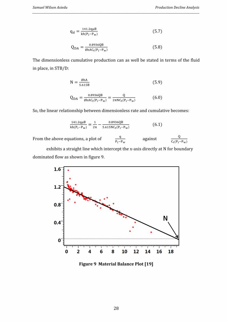
From the above equations, a plot of q
Pi−Pw against
Q
Ct(Pi−Pw)
exhibits a straight line which intercept the x-axis directly at N for boundary
dominated flow as shown in figure 9.
Figure 9 Material Balance Plot [19]
Samuel Wilson Asiedu Production Decline Analysis ______________________________________________________________________________________________________________________
29
3 Methodology
3.1 Introduction
As discussed earlier, the petroleum industry is masked by huge financial
commitments. This makes it necessary for production performance forecast of the
reservoir property towards making good and quality decisions. In a field, after some
years of production, information about the depletion and historical performance can
be used as a benchmark to gain understanding into the future production
performance if well’s production strategy remains unaltered.
In this work, numerical reservoir simulations were applied to build a synthetic
reservoir model that represents the static and dynamic performance of the reservoir.
This numerical model is built on series of mathematical equations, sets of
assumptions, initial and boundary conditions and the purpose to which it was
employed in terms of operating conditions. Schlumberger’s commercialized software,
ECLIPSE was the numerical simulator used in this research work. Ecrin’s TOPAZE
software (commercialized by KAPPA Engineering) was used to provide analytical
interpretation of the numerically simulated production data obtained from ECLIPSE.
The reason for assuming a numerical simulator and an analytical software is for the
fact that it acts as a dependable and flexible tool to identify optimum production and
management approaches by developing several operating scenarios. Due to lack of
real life data, a complete set of synthetic data with reservoir, fluid and production
properties was employed. Again, the synthetic data provides the opportunity to make
sensitivity analysis on significant parameters.
The production data (time function of rate and pressures) used for the rate transient
analysis is generated by the numerical simulator. The decline curve analysis was then
performed analytically to make a production forecast and obtain the reservoir
parameters that contributed to the rate decline. For the purpose of our study, a base
case scenario was considered which is described here in this chapter. This work
seeks out to investigate the integrity of the various developments in forecasting
production performance, their strengths and weaknesses, when to and when not to
apply a method. In this case, the traditional Arps methods as well as several modern
Samuel Wilson Asiedu Production Decline Analysis ______________________________________________________________________________________________________________________
30
methods were investigated to identify coherence and limitations. Details of the
simulation workflow and computations are described in this chapter.
3.2 Synthetic Reservoir Model
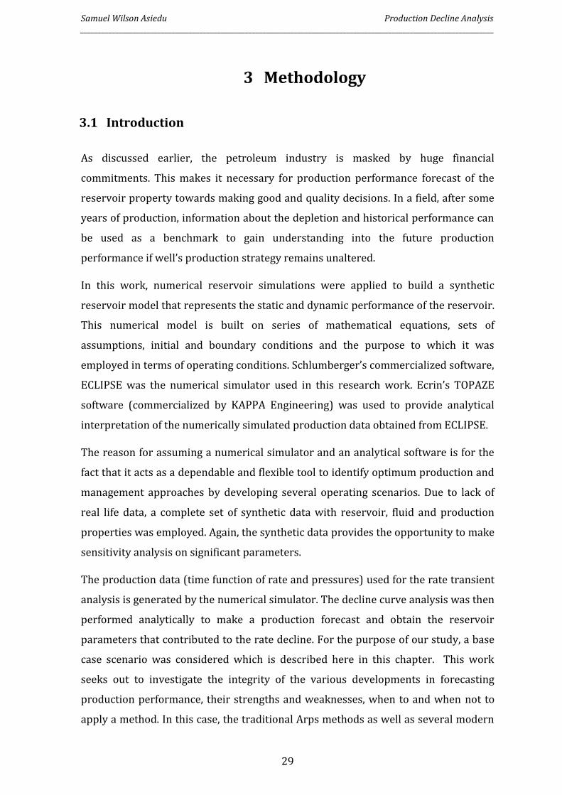
To obtain production data used for our analysis, Schlumberger’s Eclipse 100 (Black
Oil) Simulator was used to model a synthetic rectangular reservoir. An
undersaturated oil reservoir with initial pressure (Pi) of about 5000 psi at a datum
depth, 8000 ft ss and a reservoir temperature of 212oF. The reservoir is made up of
1200 active grid cells, 20 each in the x and y direction, and 3 in the z direction as
shown in figure 10. Each cell has dimension 300ft by 300ft by 50ft in the x, y and z
direction respectively. The reservoir top is at a depth of 8000 ft ss. The reservoir is
100% saturated with oil, such that, there is no irreducible water saturation. The Oil-
Water contact (OWC) is positioned at a depth of 9000ft ss, far below the bottommost
depth and that stands to mean that the reservoir is producing under depletion drive
mechanism.
Figure 10 3D Reservoir Geometry
The reservoir is homogeneous and isotropic with a single vertical production well of
radius, 0.328 ft placed at the center of the square-shaped bounded geometry (10,10)
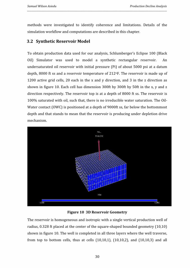
shown in figure 10. The well is completed in all three layers where the well traverse,
from top to bottom cells, thus at cells (10,10,1), (10,10,2), and (10,10,3) and all
Samuel Wilson Asiedu Production Decline Analysis ______________________________________________________________________________________________________________________
31
completed cells are open to production as shown in figure 11. The well is producing
at a constant bottomhole flowing pressure of 3200 psia, which is sometimes known
as the critical bottomhole pressure (Pwfc).
Figure 11 Reservoir Completion
3.3 PVT and Petrophysical Properties
The reservoir, fluid and rock properties defined at a reference pressure of 5000 psia
are summarized in the table below;
Table 3 Rock and Fluid Properties
Reservoir Fluid Properties Values
Oil Gravity 30 oAPI
Oil Viscosity (µo) 1.0842 cp
Oil Formation Volume Factor (Boi) 1.2487 rb/stb
Oil Saturation (So) 1.0000
Water Saturation (Sw) 0.0000
Water Formation Volume Factor (Bw) 1.0050 rb/stb
Water Compressibility 2.5E-06 psi-1
Constant Flowing Bottomhole Pressure (Pwfc)
3200 psia
Reservoir Rock Properties
Samuel Wilson Asiedu Production Decline Analysis ______________________________________________________________________________________________________________________
32
Formation compressibility (Cf) 3.8E-06 psi-1
Porosity (ø) 0.2300
Total Compressibility (Ct) 1.1809E-05 psi-1
Net to Gross Ratio (NTG) 1.0000
Permeability (K) 100 mD
Pay Zone Thickness (h) 150 ft
Transmissibility (Kh) 15000 mD.ft
No Flow Boundaries (North, South, East, West)
3000 ft
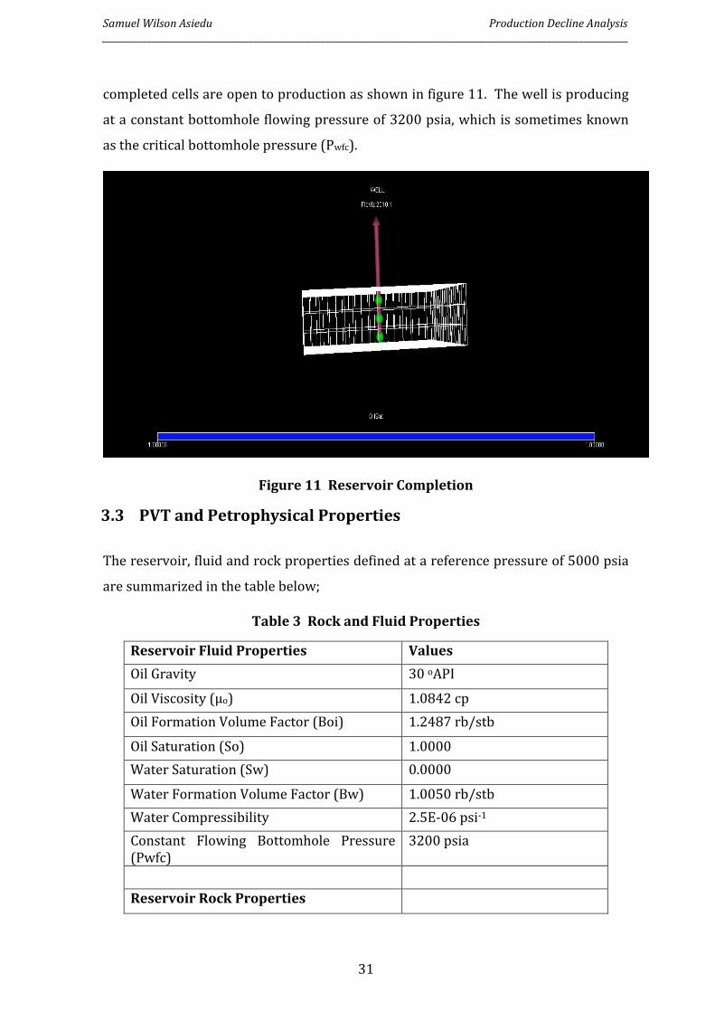
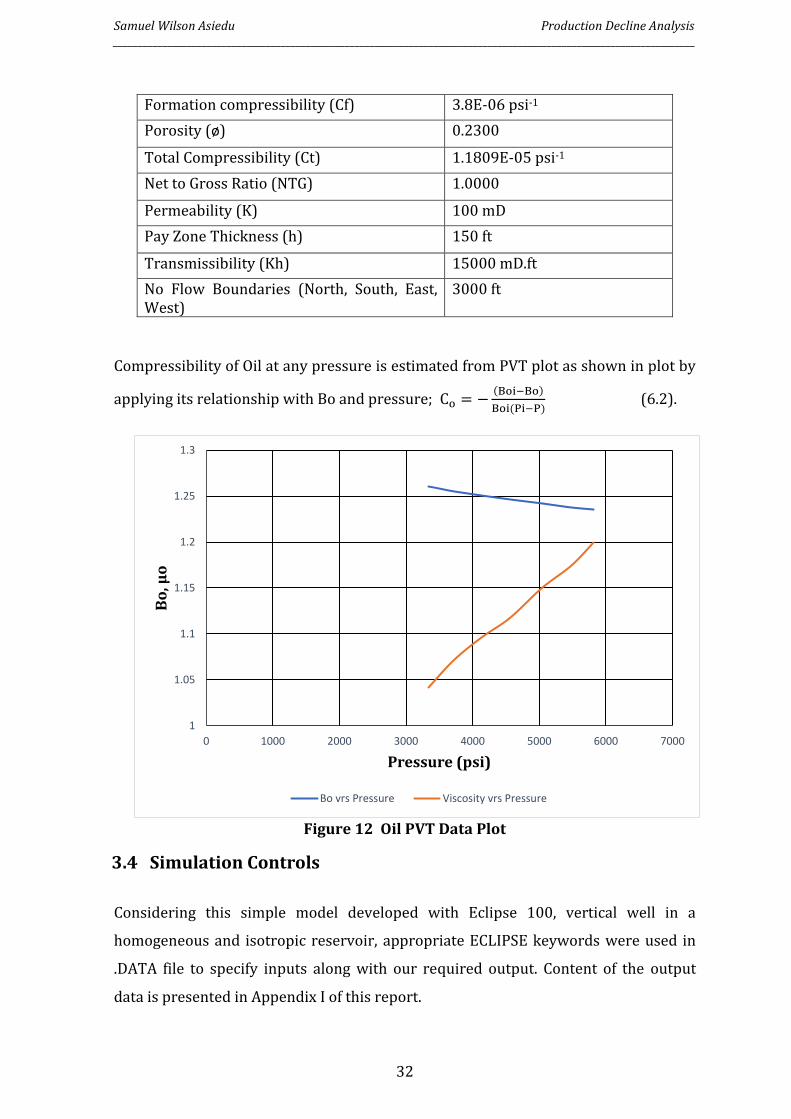
Compressibility of Oil at any pressure is estimated from PVT plot as shown in plot by
applying its relationship with Bo and pressure; Co = −(Boi−Bo)
Boi(Pi−P) (6.2).
Figure 12 Oil PVT Data Plot
3.4 Simulation Controls
Considering this simple model developed with Eclipse 100, vertical well in a
homogeneous and isotropic reservoir, appropriate ECLIPSE keywords were used in
.DATA file to specify inputs along with our required output. Content of the output
data is presented in Appendix I of this report.
1
1.05
1.1
1.15
1.2
1.25
1.3
0 1000 2000 3000 4000 5000 6000 7000
Bo
, µo
Pressure (psi)
Bo vrs Pressure Viscosity vrs Pressure
Samuel Wilson Asiedu Production Decline Analysis ______________________________________________________________________________________________________________________
33
SCHEDULE section of the eclipse dataset defines the well data and production
schedule. The WELSPECS keyword defines the specifications of the well by describing
its name and the position of the wellhead, its bottomhole reference depth and other
specification data. COMPDAT keyword was used to specify where the well was
placed, and the connections opened to flow from the reservoir. This keyword was
also used to specify the wellbore diameter. In order to generate the outcome of a
declining oil well, the well control used was BHP instead of ORAT such that the well
produces at the constant bottomhole pressure (Pwf). The simulator was set to give an
output report every 10 days interval, continuously for 1850 days of production and
thus our decline was monitored for about 5 years. Several output parameters were
requested to be reported after each time step but the most relevant of it were;
1. Well Oil Production Rate, WOPR (STB/D)
2. Well Oil Production Total, WOPT (STB)
3. Well Bottomhole Pressure, WBHP (psia)
4. Field Oil in Place, FOIP (STB)
The Field Oil in Place requested from the simulation run was used as a means of
verifying the correctness of the analytical model built from Ecrin’s Topaze.
3.5 Application of Arps Empirical Model
The parameters required for the Arps model were the time interval in years, Well Oil
Production Rate and the Well Oil Production Total. The conventional Arps model uses
the rate history data alone without the pressure history. After the simulation run was
completed, the 5 years production data were reported on the .RSM file and exported
to EXCEL.
Data from the first year of production was extracted and was used to identify the
model that best suites the decline and was consequently used to determine the
decline parameters. In this case, we chose the first year of production as the historical
data and was then used to forecast the production for the following two years.
Data quality and resolution has been found to be one of the set-backs of the Arps
Empirical Model application, such that, a short-term data cannot be evidently
ascribed to a specific model. To clear our doubts in relation to the model selected,

Samuel Wilson Asiedu Production Decline Analysis ______________________________________________________________________________________________________________________
34
two years production was also selected as history and was used to forecast the
production for the following year and fortunately, the same result was achieved.
Our data showed a complete drawdown period with no build up or intervention to
satisfy the assumption that fluid flow follows an uninterrupted condition and that,
causes that controlled the trend of the curve previously will remain same into the
future.
As summarized in figure 6, cartesian plot, semi-log and log-log plots were applied to
the production data with the aim of obtaining a straight line for an easier description
of the model unless the decline follows the hyperbolic model which will inevitably
produce a curve from all the plots. After a suitable model was identified, its
corresponding empirical equation from the hyperbolic family as listed in table 1 is
used to evaluate the initial flow rate, decline rate constant and Arps decline exponent.
3.6 Analytical Simulation in TOPAZE
3.6.1 Initialization
The analytical simulation in Ecrin’s Topaze begins with the initialization procedure
which required the input of PVT data, geometric well and the reservoir information.
Data required for our analysis include;
1. Production history
2. Pressure history
3. PVT, Correlations, tables or constraints
4. Wellbore radius
5. Porosity
6. Net vertical drained thickness
A new document is created in TOPAZE for Single Well Production Analysis and the
reservoir information is keyed in. In the PVT parameter dialog opened, the formation
volume factor and viscosities are computed from PVT table used in the numerical
simulation. Compressibility is selected to be correlated from the formation volume
factor table. Setting this up makes the document ready for analysis.
TOPAZE makes use of the available data thus both rate and pressure histories. For
our analysis, two years production history is imported from the EXCEL spreadsheet
Samuel Wilson Asiedu Production Decline Analysis ______________________________________________________________________________________________________________________
35
obtained from the numerical simulation and loaded into the new document created
in TOPAZE. After the data upload, the software uses the production history to
generate the cumulative production automatically. Pressure data is also loaded and
displayed in the history plot. The analysis page now displays production data on top
the pressure data in a single window.
3.6.2 Data Extraction and Diagnostics
After data has been synchronized, analysis begin by using the extraction button to
select the step amount of rate and pressure gauge for interpretation within a defined
range of time. The selected time range will be same for both pressure and rate
histories. In addition to the history data, other plots generated by the software
include;
1. Fetkovish plot and its type curves
2. Blasingame plot and its type curves
3. The log-log plot
4. Normalized Rate-Cumulative plot
3.6.3 Model Generation
After the diagnostics, analytical models are selected as we try to simultaneously
obtain a match between the models and the real data in all applicable plots including
the history plot. Knowledge of the well configuration and the reservoir was used as a
contrast between the real and the model. The model parameters were finally varied
until a realistic match was obtained.
3.6.4 Production Forecast and Sensitivity Analysis
A production forecast was later performed after obtaining a reasonable and realistic
match by defining a bottomhole flowing pressure. This was done to extend the model,
in terms of pressure and rate by adding to the present history for the following year.
At this point, we concluded the interpretation of the model by making sensitivity
analysis, achieved by running different values of a given parameter and display of
model generations that corresponds to it to compare with the history.
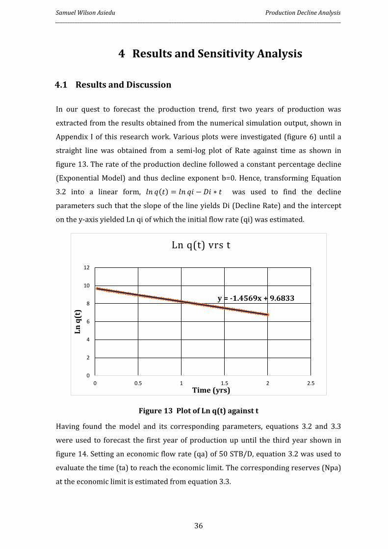
Samuel Wilson Asiedu Production Decline Analysis ______________________________________________________________________________________________________________________
36
4 Results and Sensitivity Analysis
4.1 Results and Discussion
In our quest to forecast the production trend, first two years of production was
extracted from the results obtained from the numerical simulation output, shown in
Appendix I of this research work. Various plots were investigated (figure 6) until a
straight line was obtained from a semi-log plot of Rate against time as shown in
figure 13. The rate of the production decline followed a constant percentage decline
(Exponential Model) and thus decline exponent b=0. Hence, transforming Equation
3.2 into a linear form, 𝑙𝑛 𝑞(𝑡) = 𝑙𝑛 𝑞𝑖 − 𝐷𝑖 ∗ 𝑡 was used to find the decline
parameters such that the slope of the line yields Di (Decline Rate) and the intercept
on the y-axis yielded Ln qi of which the initial flow rate (qi) was estimated.
Figure 13 Plot of Ln q(t) against t
Having found the model and its corresponding parameters, equations 3.2 and 3.3
were used to forecast the first year of production up until the third year shown in
figure 14. Setting an economic flow rate (qa) of 50 STB/D, equation 3.2 was used to
evaluate the time (ta) to reach the economic limit. The corresponding reserves (Npa)
at the economic limit is estimated from equation 3.3.
y = -1.4569x + 9.6833
0
2
4
6
8
10
12
0 0.5 1 1.5 2 2.5
Ln
q(t
)
Time (yrs)
Ln q(t) vrs t
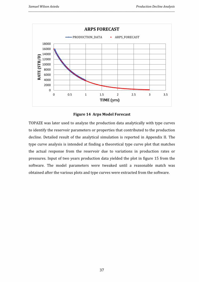
Samuel Wilson Asiedu Production Decline Analysis ______________________________________________________________________________________________________________________
37
Figure 14 Arps Model Forecast
TOPAZE was later used to analyze the production data analytically with type curves
to identify the reservoir parameters or properties that contributed to the production
decline. Detailed result of the analytical simulation is reported in Appendix II. The
type curve analysis is intended at finding a theoretical type curve plot that matches
the actual response from the reservoir due to variations in production rates or
pressures. Input of two years production data yielded the plot in figure 15 from the
software. The model parameters were tweaked until a reasonable match was
obtained after the various plots and type curves were extracted from the software.
0
2000
4000
6000
8000
10000
12000
14000
16000
18000
0 0.5 1 1.5 2 2.5 3 3.5
RA
TE
(S
TB
/D
)
TIME (yrs)
ARPS FORECAST
PRODUCTION_DATA ARPS_FORECAST
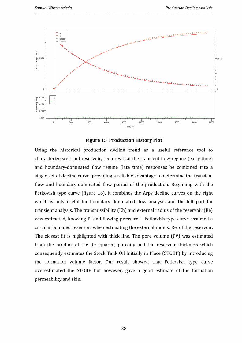
Samuel Wilson Asiedu Production Decline Analysis ______________________________________________________________________________________________________________________
38
Figure 15 Production History Plot
Using the historical production decline trend as a useful reference tool to
characterize well and reservoir, requires that the transient flow regime (early time)
and boundary-dominated flow regime (late time) responses be combined into a
single set of decline curve, providing a reliable advantage to determine the transient
flow and boundary-dominated flow period of the production. Beginning with the
Fetkovish type curve (figure 16), it combines the Arps decline curves on the right
which is only useful for boundary dominated flow analysis and the left part for
transient analysis. The transmissibility (Kh) and external radius of the reservoir (Re)
was estimated, knowing Pi and flowing pressures. Fetkovish type curve assumed a
circular bounded reservoir when estimating the external radius, Re, of the reservoir.
The closest fit is highlighted with thick line. The pore volume (PV) was estimated
from the product of the Re-squared, porosity and the reservoir thickness which
consequently estimates the Stock Tank Oil Initially in Place (STOIIP) by introducing
the formation volume factor. Our result showed that Fetkovish type curve
overestimated the STOIIP but however, gave a good estimate of the formation
permeability and skin.
0
10000
Liq
uid
ra
te [S
TB
/D]
0
2E+6
Liq
uid
vo
lum
e [S
TB
]
q
Q
q model
Q model
0 2000 4000 6000 8000 10000 12000 14000 16000 18000
Time [hr]
3200
3700
4200
4700
Pre
ssu
re [p
sia
]
Pi
p
Production history plot (Liquid rate [STB/D], Pressure [psia] vs Time [hr])
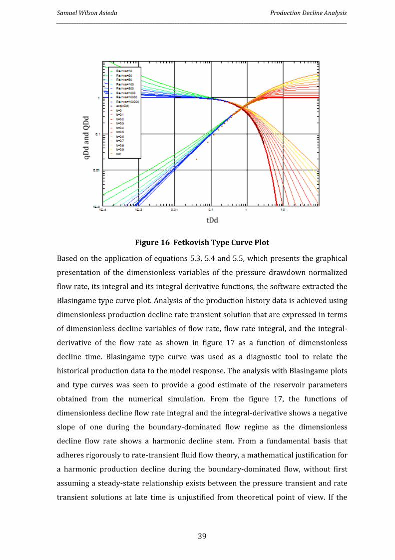
Samuel Wilson Asiedu Production Decline Analysis ______________________________________________________________________________________________________________________
39
Figure 16 Fetkovish Type Curve Plot
Based on the application of equations 5.3, 5.4 and 5.5, which presents the graphical
presentation of the dimensionless variables of the pressure drawdown normalized
flow rate, its integral and its integral derivative functions, the software extracted the
Blasingame type curve plot. Analysis of the production history data is achieved using
dimensionless production decline rate transient solution that are expressed in terms
of dimensionless decline variables of flow rate, flow rate integral, and the integral-
derivative of the flow rate as shown in figure 17 as a function of dimensionless
decline time. Blasingame type curve was used as a diagnostic tool to relate the
historical production data to the model response. The analysis with Blasingame plots
and type curves was seen to provide a good estimate of the reservoir parameters
obtained from the numerical simulation. From the figure 17, the functions of
dimensionless decline flow rate integral and the integral-derivative shows a negative
slope of one during the boundary-dominated flow regime as the dimensionless
decline flow rate shows a harmonic decline stem. From a fundamental basis that
adheres rigorously to rate-transient fluid flow theory, a mathematical justification for
a harmonic production decline during the boundary-dominated flow, without first
assuming a steady-state relationship exists between the pressure transient and rate
transient solutions at late time is unjustified from theoretical point of view. If the
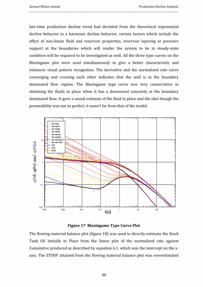
Samuel Wilson Asiedu Production Decline Analysis ______________________________________________________________________________________________________________________
40
late-time production decline trend had deviated from the theoretical exponential
decline behavior to a harmonic decline behavior, certain factors which include the
effect of non-linear fluid and reservoir properties, reservoir layering or pressure
support at the boundaries which will render the system to be in steady-state
condition will be required to be investigated as well. All the three type curves on the
Blasingame plot were used simultaneously to give a better characteristic and
enhances visual pattern recognition. The derivative and the normalized rate curve
converging and crossing each other indicates that the well is in the boundary
dominated flow regime. The Blasingame type curve was very conservative in
obtaining the fluids in place when it has a downward concavity at the boundary
dominated flow. It gave a sound estimate of the fluid in place and the skin though the
permeability was not so perfect, it wasn’t far from that of the model.
Figure 17 Blasingame Type Curve Plot
The flowing material balance plot (figure 18) was used to directly estimate the Stock
Tank Oil Initially in Place from the linear plot of the normalized rate against
Cumulative produced as described by equation 6.1, which was the intercept on the x-
axis. The STOIIP attained from the flowing material balance plot was overestimated
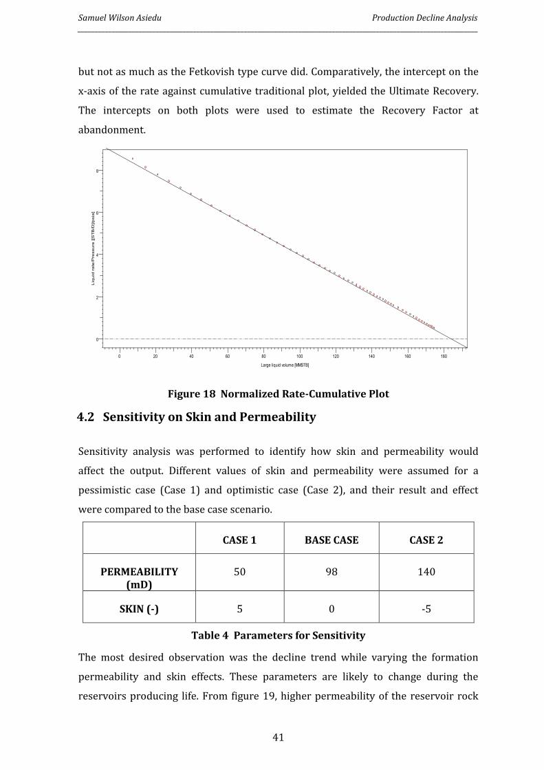
Samuel Wilson Asiedu Production Decline Analysis ______________________________________________________________________________________________________________________
41
but not as much as the Fetkovish type curve did. Comparatively, the intercept on the
x-axis of the rate against cumulative traditional plot, yielded the Ultimate Recovery.
The intercepts on both plots were used to estimate the Recovery Factor at
abandonment.
Figure 18 Normalized Rate-Cumulative Plot
4.2 Sensitivity on Skin and Permeability
Sensitivity analysis was performed to identify how skin and permeability would
affect the output. Different values of skin and permeability were assumed for a
pessimistic case (Case 1) and optimistic case (Case 2), and their result and effect
were compared to the base case scenario.
CASE 1 BASE CASE CASE 2
PERMEABILITY (mD)
50 98 140
SKIN (-) 5 0 -5
Table 4 Parameters for Sensitivity
The most desired observation was the decline trend while varying the formation
permeability and skin effects. These parameters are likely to change during the
reservoirs producing life. From figure 19, higher permeability of the reservoir rock
0 20 40 60 80 100 120 140 160 180
Large liquid volume [MMSTB]
0
2
4
6
8
Liq
uid
ra
te/P
ress
ure
[[S
TB
/D]/p
sia
]
Normalized Rate-Cumulative: q/(Pi-Pwf) [[STB/D]/psia] vs Q/Ct/(Pi-Pwf) [MMSTB]
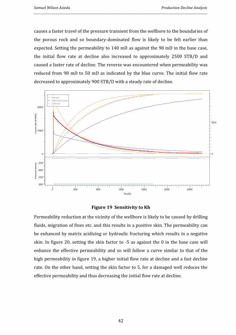
Samuel Wilson Asiedu Production Decline Analysis ______________________________________________________________________________________________________________________
42
causes a faster travel of the pressure transient from the wellbore to the boundaries of
the porous rock and so boundary-dominated flow is likely to be felt earlier than
expected. Setting the permeability to 140 mD as against the 98 mD in the base case,
the initial flow rate at decline also increased to approximately 2500 STB/D and
caused a faster rate of decline. The reverse was encountered when permeability was
reduced from 98 mD to 50 mD as indicated by the blue curve. The initial flow rate
decreased to approximately 900 STB/D with a steady rate of decline.
Figure 19 Sensitivity to Kh
Permeability reduction at the vicinity of the wellbore is likely to be caused by drilling
fluids, migration of fines etc. and this results in a positive skin. The permeability can
be enhanced by matrix acidizing or hydraulic fracturing which results in a negative
skin. In figure 20, setting the skin factor to -5 as against the 0 in the base case will
enhance the effective permeability and so will follow a curve similar to that of the
high permeability in figure 19, a higher initial flow rate at decline and a fast decline
rate. On the other hand, setting the skin factor to 5, for a damaged well reduces the
effective permeability and thus decreasing the initial flow rate at decline.
0
10000
20000
Liq
uid
ra
te [S
TB
/D]
0
2E+6
Liq
uid
vo
lum
e [S
TB
]
7500 md.ft
14690.9 md.ft (current)
21000 md.ft
0 4000 8000 12000 16000 20000 24000
Time [hr]
3200
3700
4200
4700
Pre
ssu
re [p
sia
]
Sensitivity to k.h (Liquid volume [STB], Pressure [psia] vs Time [hr])
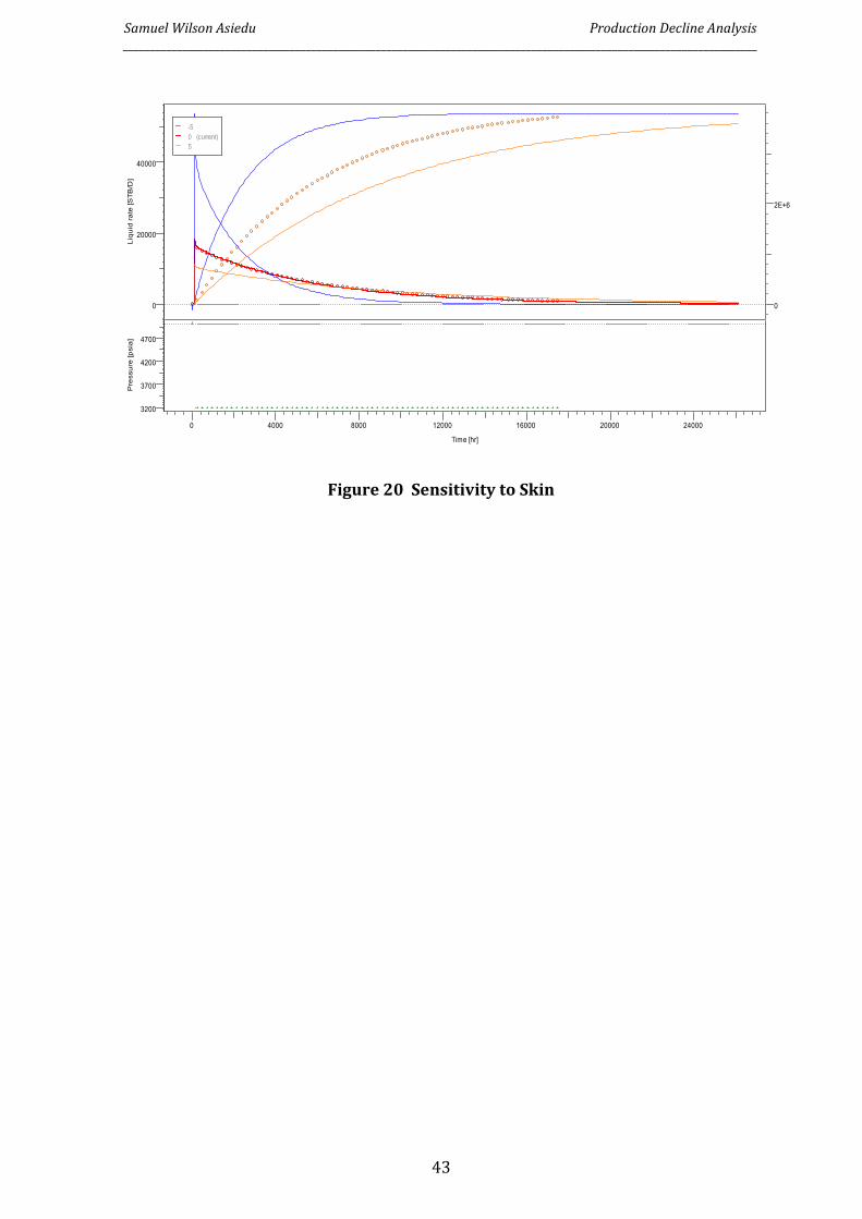
Samuel Wilson Asiedu Production Decline Analysis ______________________________________________________________________________________________________________________
43
Figure 20 Sensitivity to Skin
0
20000
40000
Liqu
id ra
te [S
TB/D
]
0
2E+6
Liqu
id v
olum
e [S
TB]
-5
0 (current)
5
0 4000 8000 12000 16000 20000 24000
Time [hr]
3200
3700
4200
4700
Pre
ssur
e [p
sia]
Sensitivity to Skin (Liquid volume [STB], Pressure [psia] vs Time [hr])
Samuel Wilson Asiedu Production Decline Analysis ______________________________________________________________________________________________________________________
44
5 Conclusion
Throughout this work, a comprehensive approach for the interpretation of
production data for predicting the long-term production of a producing well while
using same data as a means of diagnosing the reservoir characteristics. Various
methods have been discussed with their diagnostic plots and characteristic
signatures on each plot.
The Arps traditional method was successfully applied to forecast the historical
production data and to estimate the reserves. However, the method should not be
absolutely relied on since it may overestimate or underestimate the reserves due to
the fact that it ignores the pressure data, though it gives a reasonable approximation
of the reserves. Seen from our results, as shown in Table 5 the Arps Exponential
method overestimated the cumulative produced. Moreover, for transient production
data, this method cannot be applied since it only works for boundary-dominated
flows. The b value was expected to be zero (b=0) since it had already been stated
categorically that, the reservoir was producing by depletion drive and nothing more
could have been expected other than an exponential decline and more so producing
at constant operating conditions of pressure and variable rate.
On the basis of comparison (Table 5), the Blasingame type curve plot was seen to
provide a good estimate of the fluid in place as well as the parameters contributing to
the reservoir response. However, the Fetkovish type curve gave a close estimate of
the permeability than that of the Blasingame type curve, though not by any wide
margin.
In this study, application of both numerical simulation and rate transient analytical
methods using commercialized software, Schlumberger’s Eclipse and Ecrin TOPAZE
from KAPPA helped to comprehend the effect of reservoir parameters on the
inconsistencies in our imposed values.
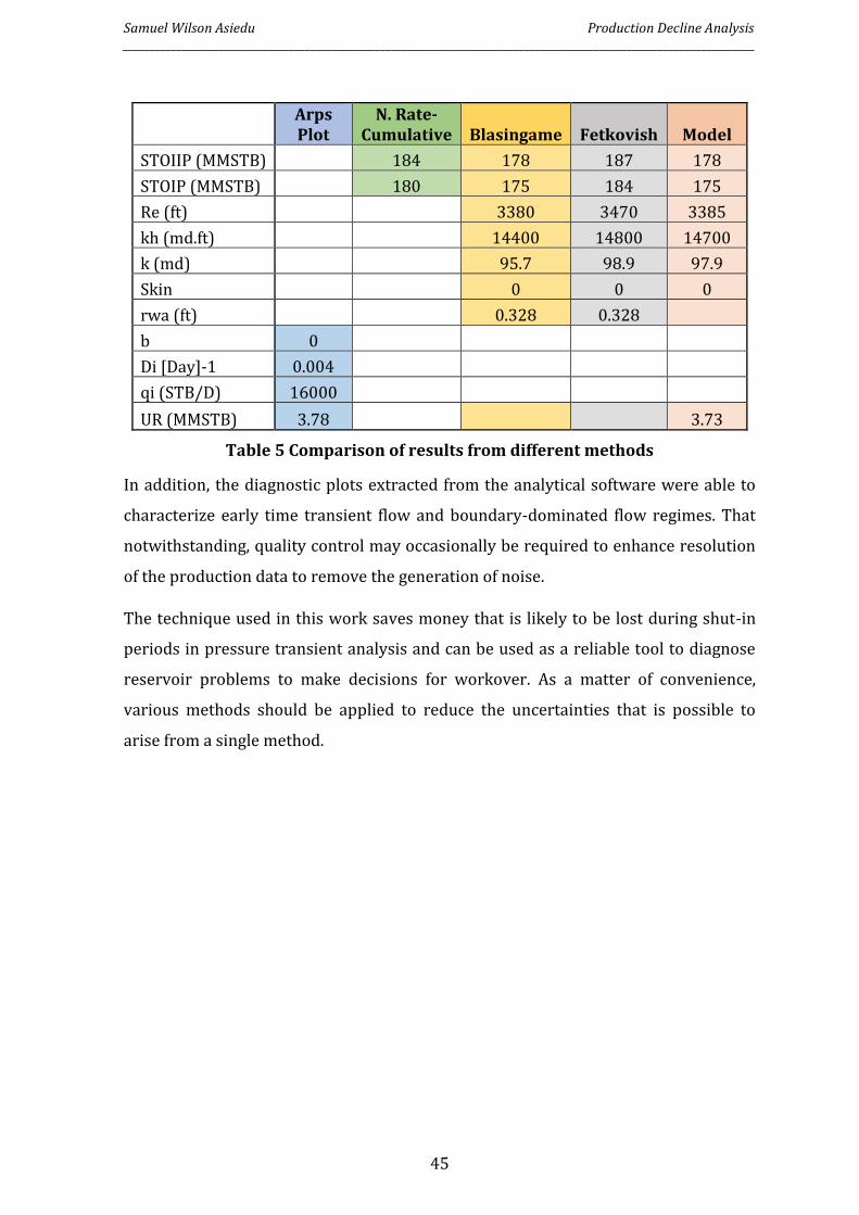
Samuel Wilson Asiedu Production Decline Analysis ______________________________________________________________________________________________________________________
45
Arps Plot
N. Rate-Cumulative Blasingame Fetkovish Model
STOIIP (MMSTB) 184 178 187 178
STOIP (MMSTB) 180 175 184 175
Re (ft) 3380 3470 3385
kh (md.ft) 14400 14800 14700
k (md) 95.7 98.9 97.9
Skin 0 0 0
rwa (ft) 0.328 0.328
b 0
Di [Day]-1 0.004
qi (STB/D) 16000
UR (MMSTB) 3.78 3.73
Table 5 Comparison of results from different methods
In addition, the diagnostic plots extracted from the analytical software were able to
characterize early time transient flow and boundary-dominated flow regimes. That
notwithstanding, quality control may occasionally be required to enhance resolution
of the production data to remove the generation of noise.
The technique used in this work saves money that is likely to be lost during shut-in
periods in pressure transient analysis and can be used as a reliable tool to diagnose
reservoir problems to make decisions for workover. As a matter of convenience,
various methods should be applied to reduce the uncertainties that is possible to
arise from a single method.

Samuel Wilson Asiedu Production Decline Analysis ______________________________________________________________________________________________________________________
46
6 References
[1] H. M, D. S, T. X and J. S, "Decline and depletion rates of oil production: a
comprehensive investigation," Philosophical transactions of the royal society, p.
0448, 2014.
[2] T. Ahmed and P. McKinney, "Decline Curve Analysis," in Advanced Reservoir
Engineering, Gulf Professional Publishing, 2005, pp. 237-264.
[3] H. Sun, Advanced Production Decline Analysis and Application, H. Sun, Ed.,
Elsevier, 2015.
[4] International Energy Agency, "World energy outlook," 2008. [Online]. Available:
http://www. worldenergyoutlook.org/publications/2008-1994/.
[5] S. A, I. GM and B. JL, Practical enhanced reservoir engineering, Tulsa: Pennwell
Books, 2008.
[6] T. E, G. A, G. C. C and P. S. D, "Enhanced Oil Recovery using Carbon Dioxide in the
European Energy System," European Commission Joint Research Center.
[7] R. Amit, "Petroleum reservoir exploitation: switching from primary to
secondary recovery," Oper. Res, vol. 34, pp. 534-549, 1986.
[8] F. Robelius, "Giant oil fields: the highway to oil: giant oil fields and their
importance for future oil production," Doctoral thesis, Uppsala University,
Sweden, 2007.
[9] A. Muggeridge, A. Cockin, K. Webb, H. Frampton, I. Collins, T. Moulds and P.
Salino, "Recovery rates, enhanced oil recovery and technological limits," Phil.
Trans. R. Soc, vol. A 372, 2014.
[10] H. M, . S. B, . J. K and A. K, " The evolution of giant oil field production
behaviour," Natural Resources Research, vol. 18, no. March, pp. 39-56, 2009.
Samuel Wilson Asiedu Production Decline Analysis ______________________________________________________________________________________________________________________
47
[11] M. Höök, "Depletion rate analysis of fields and regions: A methodological
foundation," Fuel, vol. 121, pp. 95-108, 2014.
[12] S. W. a. P. B. D. Poston, Analysis of Production Decline Curves, Richardson:
Society of Petroleum Engineers, 2007.
[13] H. Slider, Worldwide Practical Petroleum Reservoir Engineering Methods,
Pennwell Publishing Company, 1983.
[14] Arps and J. J, "Analysis of Decline Curves," Transactions of the American Institute
of Mining, Metallurgical and Petroleum Engineers, pp. 160,228-247, 1945.
[15] A. A. Hamouda, "Production Technology," Stavanger, 2015.
[16] A. J. Clark, Decline Curve Analysis in Unconventional Resource Play using
Logistic Growth Models, The University Texas at Austin, 2011.
[17] L. Lund, "Decline Curve Analysis of Shale Oil Production," Uppsala Universitet,
Uppsala, 2014.
[18] D. A. (. A. I. L. Mattar, "A Systematic and Comprehensive Methodology for
Advanced Analysis of Production Data," in SPE Annual Technical Conference and
Exhibition, Denver, Colorado, 2003.
[19] O. Houze, D. Viturat, O. S. Fjaere and (. al), Dynamic Data Analysis; The theory
and practice of Pressure Transient, Production Analysis, Well Performance
Analysis, Production Logging and the use of Permanent Downhole Gauge Data,
KAPPA, 1988-2012.
[20] Fekete, "Fetkovich Typecurve Analysis Theory," 2014. [Online]. Available:
http://www.fekete.com/SAN/WebHelp/FeketeHarmony/Harmony_WebHelp/
Content/HTML_Files/Reference_Material/Analysis_Method_Theory/Fetkovich_
Theory.htm. [Accessed September 2017].
[21] PetroWiki, "Types of decline analysis in production forecasting," 2012. [Online].
Available:
http://petrowiki.org/Types_of_decline_analysis_in_production_forecasting.
Samuel Wilson Asiedu Production Decline Analysis ______________________________________________________________________________________________________________________
48
[Accessed September 2017].
[22] T. A. M. T. L. &. L. W. J. Blasingame, "Decline Curve Analysis for Variable
Pressure Drop/Variable Flowrate Systems," OnePetro, 1 January 1991.
[23] J. a. T. B. Palacio, "Decline-Curve Analysis Using Type Curves - Analysis of Gas
Well Production Data," in SPE Joint Rocky Mountain Regional and Low
Permeability Reservoirs Symposium, Denver, CO, 1993.
[24] D. A. J. A. &. P. Y. M. Bourdet, "Use of Pressure Derivative in Well Test
Interpretation," OnePetro, no. Paper SPE 12777, 1 June 1989.
[25] A. H. C. OPT, "http://www.optpt.com/prodforecastgas/," Optimization
Petroleum Technologies, [Online]. Available:
http://optpt.com/imgs/modules/ProdForecastGas_5.jpg. [Accessed 9 October
2017].
[26] R. G. D. S. &. F. D. Agarwal, "Analyzing Well Production Data Using Combined-
Type-Curve Analysis and Decline-Curve-Analysis Concepts," OnePetro.org, vol.
2, no. 05, 1 October 1991.
[27] Fekete, "Agarwal-Gardner Typecurve Analysis Theory," 2014. [Online].
Available:
http://www.fekete.com/SAN/WebHelp/FeketeHarmony/Harmony_WebHelp/
Content/HTML_Files/Reference_Material/Analysis_Method_Theory/Agarwal-
Gardner_Theory.htm. [Accessed Tuesday September 2017].
[28] A. Adasani and B. Bai, "Analysis of EOR projects and updated screening criteria,"
J. Pet. Sci. Eng, vol. 79, pp. 10-24, 2011.
[29] Z. L. C. &. K. M. Wang, "Validation and Extension of Asymptotic Solutions of
Diffusivity Equation and Their Applications to Synthetic Cases," OnePetro, 20
February 2017.
[30] A. T. M. S. H. M. H. M. Istiak Hussain, "Dynamic Material Balance Study of Gas
Reservoir Using Production Data: A Case Study of New Gas Sand of Kailashtila
Gas Field," International Journal of Oil, Gas and Coal Engineering. , vol. 4, no. 4,

Samuel Wilson Asiedu Production Decline Analysis ______________________________________________________________________________________________________________________
49
pp. 38-44, 2016.
APPENDIX I
Simulation Data Output & Arps Exponential Model
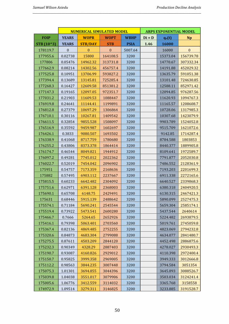
Samuel Wilson Asiedu Production Decline Analysis ______________________________________________________________________________________________________________________
50
NUMERICAL SIMULATED MODEL ARPS EXPONENTIAL MODEL
FOIP YEARS WOPR WOPT WBHP Di = D qo(t) Np
STB (10^3) YEARS STB/DAY STB PSIA 1.46 16000
178119.7 0 0 0 5007.64 16000 0
177955.6 0.02738 15800 164108.5 3200 15373.04 156739.78
177806 0.05476 14962.32 313731.8 3200 14770.67 307332.34
177662.9 0.08214 14302.56 456757.4 3200 14191.88 452029.32
177525.8 0.10951 13706.99 593827.2 3200 13635.79 591051.38
177394.4 0.13689 13145.81 725285.4 3200 13101.48 724630.85
177268.3 0.16427 12609.58 851381.2 3200 12588.11 852971.42
177147.3 0.19165 12097.05 972351.7 3200 12094.85 976287.56
177031.2 0.21903 11609.53 1088447 3200 11620.93 1094767.3
176919.8 0.24641 11144.41 1199891 3200 11165.57 1208608.7
176812.8 0.27379 10697.29 1306864 3200 10728.06 1317985.3
176710.1 0.30116 10267.81 1409542 3200 10307.68 1423079.9
176611.5 0.32854 9855.528 1508097 3200 9903.789 1524052.8
176516.9 0.35592 9459.987 1602697 3200 9515.709 1621072.6
176426.1 0.3833 9080.507 1693502 3200 9142.85 1714287.4
176338.9 0.41068 8717.759 1780680 3200 8784.588 1803853
176255.2 0.43806 8373.378 1864414 3200 8440.377 1889905.8
176174.7 0.46544 8049.821 1944912 3200 8109.641 1972589.7
176097.2 0.49281 7745.012 2022362 3200 7791.877 2052030.8
176022.7 0.52019 7454.042 2096902 3200 7486.552 2128361.9
175951 0.54757 7173.359 2168636 3200 7193.203 2201699.3
175882 0.57495 6903.112 2237667 3200 6911.338 2272165.6
175815.5 0.60233 6642.482 2304092 3200 6640.527 2339868.3
175751.6 0.62971 6391.128 2368003 3200 6380.318 2404920.5
175690.1 0.65708 6148.75 2429491 3200 6130.315 2467421.3
175631 0.68446 5915.139 2488642 3200 5890.099 2527475.3
175574.1 0.71184 5690.241 2545544 3200 5659.304 2585174.1
175519.4 0.73922 5473.541 2600280 3200 5437.544 2640614
175466.7 0.7666 5264.65 2652926 3200 5224.482 2693879.5
175416.1 0.79398 5063.401 2703560 3200 5019.761 2745059.8
175367.4 0.82136 4869.485 2752255 3200 4823.069 2794232.8
175320.6 0.84873 4683.304 2799088 3200 4634.077 2841480.7
175275.5 0.87611 4503.209 2844120 3200 4452.498 2886875.6
175232.3 0.90349 4328.29 2887403 3200 4278.027 2930493.3
175190.7 0.93087 4160.826 2929012 3200 4110.398 2972400.4
175150.7 0.95825 3999.358 2969005 3200 3949.333 3012666.8
175112.2 0.98563 3844.235 3007448 3200 3794.584 3051354
175075.3 1.01301 3694.855 3044396 3200 3645.893 3088526.7
175039.8 1.04038 3551.017 3079906 3200 3503.034 3124241.4
175005.6 1.06776 3412.559 3114032 3200 3365.768 3158558
174972.9 1.09514 3279.311 3146825 3200 3233.885 3191528.7

Samuel Wilson Asiedu Production Decline Analysis ______________________________________________________________________________________________________________________
51
174941.3 1.12252 3151.094 3178336 3200 3107.166 3223208.6
174911.1 1.1499 3027.732 3208613 3200 2985.416 3253646
174882 1.17728 2909.054 3237704 3200 2868.433 3282891.8
174854 1.20465 2794.894 3265653 3200 2756.037 3310990.7
174827.2 1.23203 2685.09 3292504 3200 2648.042 3337989.5
174801.4 1.25941 2579.485 3318298 3200 2544.282 3363929.4
174776.6 1.28679 2477.928 3343078 3200 2444.585 3388853.8
174752.8 1.31417 2380.272 3366880 3200 2348.797 3412800.7
174730 1.34155 2286.375 3389744 3200 2256.76 3435810
174708 1.36893 2196.098 3411705 3200 2168.332 3457917
174686.9 1.3963 2109.31 3432798 3200 2083.366 3479158.5
174666.6 1.42368 2025.881 3453057 3200 2001.732 3499566.9
174647.2 1.45106 1945.686 3472514 3200 1923.295 3519176.3
174628.5 1.47844 1868.606 3491200 3200 1847.933 3538016.7
174610.5 1.50582 1794.524 3509145 3200 1775.522 3556119.5
174593.3 1.5332 1723.328 3526378 3200 1705.951 3573512.3
174576.8 1.56058 1654.909 3542928 3200 1639.103 3590224.2
174560.9 1.58795 1589.163 3558819 3200 1574.877 3606280.7
174545.6 1.61533 1525.989 3574079 3200 1513.166 3621708.6
174531 1.64271 1465.289 3588732 3200 1453.875 3636531.4
174516.9 1.67009 1406.969 3602802 3200 1396.905 3650773.9
174503.4 1.69747 1350.94 3616311 3200 1342.169 3664457.8
174490.4 1.72485 1297.112 3629282 3200 1289.576 3677606
174478 1.75222 1245.403 3641736 3200 1239.046 3690238.5
174466 1.7796 1195.73 3653694 3200 1190.494 3702376.5
174454.5 1.80698 1148.015 3665174 3200 1143.845 3714038.9
174443.5 1.83436 1102.184 3676196 3200 1099.025 3725243.8
174432.9 1.86174 1058.163 3686777 3200 1055.959 3736010.1
174422.8 1.88912 1015.882 3696936 3200 1014.583 3746354.2
174413 1.9165 975.2745 3706689 3200 974.8268 3756293.3
174403.6 1.94387 936.2749 3716052 3200 936.6297 3765842.6
174394.7 1.97125 898.8209 3725040 3200 899.9279 3775018
174386 1.99863 862.8522 3733668 3200 864.6655 3783833.6
174377.7 2.02601 828.3112 3741951 3200 830.7836 3792304.1
174369.8 2.05339 795.1418 3749903 3200 798.2306 3800442.4
174362.2 2.08077 763.2907 3757536 3200 766.952 3808262
174354.8 2.10815 735.5416 3764891 3200 736.9001 3815775
174347.7 2.13552 705.3469 3771944 3200 708.0247 3822993.8
174341 2.1629 677.1795 3778716 3200 680.2818 3829929.6
174334.5 2.19028 649.8374 3785215 3200 653.625 3836593.8
174328.2 2.21766 623.7424 3791452 3200 628.0136 3842996.6
174322.3 2.24504 598.6023 3797438 3200 603.4049 3849148.8
174316.5 2.27242 574.5234 3803184 3200 579.7614 3855059.6
174311 2.2998 551.3734 3808697 3200 557.0435 3860739.1
174305.7 2.32717 529.1736 3813989 3200 535.2165 3866195.9
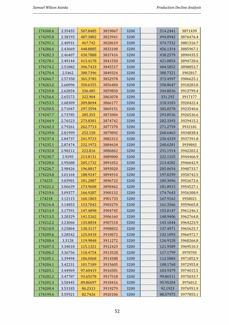
Samuel Wilson Asiedu Production Decline Analysis ______________________________________________________________________________________________________________________
52
174300.6 2.35455 507.8485 3819067 3200 514.2441 3871439
174295.8 2.38193 487.3882 3823941 3200 494.0942 3876476.4
174291.1 2.40931 467.742 3828619 3200 474.7332 3881316.7
174286.6 2.43669 448.8885 3833108 3200 456.1314 3885967.1
174282.3 2.46407 430.7888 3837416 3200 438.2579 3890435.5
174278.1 2.49144 413.4178 3841550 3200 421.0854 3894728.6
174274.2 2.51882 396.7433 3845517 3200 404.5852 3898853.7
174270.4 2.5462 380.7396 3849324 3200 388.7321 3902817
174266.7 2.57358 365.3785 3852978 3200 373.4997 3906625.1
174263.2 2.60096 350.6355 3856484 3200 358.8647 3910283.8
174259.8 2.62834 336.485 3859850 3200 344.8026 3913799.4
174256.6 2.65572 322.904 3863078 3200 331.292 3917177
174253.5 2.68309 309.8694 3866177 3200 318.3103 3920422.4
174250.5 2.71047 297.3594 3869151 3200 305.8378 3923540.6
174247.7 2.73785 285.353 3872004 3200 293.8536 3926536.6
174244.9 2.76523 273.8301 3874742 3200 282.3393 3929415.2
174242.3 2.79261 262.7713 3877370 3200 271.2759 3932181
174239.8 2.81999 252.158 3879892 3200 260.6463 3934838.4
174237.4 2.84737 241.9723 3882312 3200 250.4329 3937391.8
174235.1 2.87474 232.1972 3884634 3200 240.6201 3939845
174232.8 2.90212 222.816 3886862 3200 231.1914 3942202.2
174230.7 2.9295 213.8131 3889000 3200 222.1325 3944466.9
174228.6 2.95688 205.1732 3891052 3200 213.4282 3946642.9
174226.7 2.98426 196.8817 3893020 3200 205.0654 3948733.7
174224.8 3.01164 188.9247 3894910 3200 197.0299 3950742.5
174223 3.03901 181.2887 3896722 3200 189.3096 3952672.6
174221.2 3.06639 173.9608 3898462 3200 181.8915 3954527.1
174219.6 3.09377 166.9287 3900132 3200 174.7643 3956308.9
174218 3.12115 160.1803 3901733 3200 167.9162 3958021
174216.4 3.14853 153.7043 3903270 3200 161.3366 3959665.8
174214.9 3.17591 147.4898 3904745 3200 155.0147 3961246.3
174213.5 3.20329 141.5262 3906160 3200 148.9406 3962764.8
174212.2 3.23066 135.8034 3907518 3200 143.1044 3964223.9
174210.9 3.25804 130.3117 3908822 3200 137.4971 3965625.7
174209.6 3.28542 125.0418 3910072 3200 132.1093 3966972.7
174208.4 3.3128 119.9848 3911272 3200 126.9328 3968266.8
174207.3 3.34018 115.1321 3912423 3200 121.9589 3969510.3
174206.2 3.36756 110.4754 3913528 3200 117.1799 3970705
174205.1 3.39494 106.0068 3914588 3200 112.5884 3971852.9
174204.1 3.42231 101.7189 3915605 3200 108.1768 3972955.8
174203.1 3.44969 97.60419 3916581 3200 103.9379 3974015.5
174202.2 3.47707 93.65578 3917518 3200 99.86511 3975033.7
174201.3 3.50445 89.86697 3918416 3200 95.95204 3976012
174200.4 3.53183 86.2313 3919279 3200 92.1923 3976951.9
174199.6 3.55921 82.7426 3920106 3200 88.57975 3977855.1
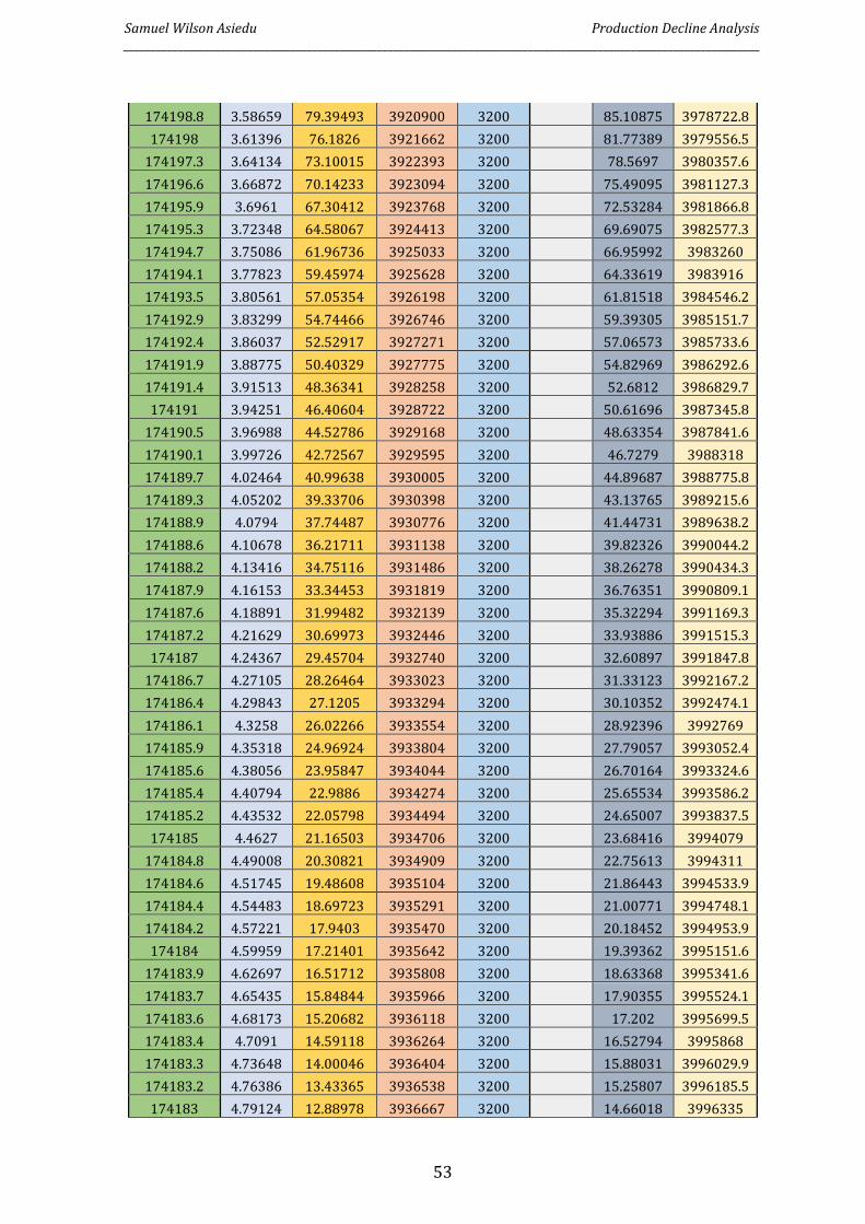
Samuel Wilson Asiedu Production Decline Analysis ______________________________________________________________________________________________________________________
53
174198.8 3.58659 79.39493 3920900 3200 85.10875 3978722.8
174198 3.61396 76.1826 3921662 3200 81.77389 3979556.5
174197.3 3.64134 73.10015 3922393 3200 78.5697 3980357.6
174196.6 3.66872 70.14233 3923094 3200 75.49095 3981127.3
174195.9 3.6961 67.30412 3923768 3200 72.53284 3981866.8
174195.3 3.72348 64.58067 3924413 3200 69.69075 3982577.3
174194.7 3.75086 61.96736 3925033 3200 66.95992 3983260
174194.1 3.77823 59.45974 3925628 3200 64.33619 3983916
174193.5 3.80561 57.05354 3926198 3200 61.81518 3984546.2
174192.9 3.83299 54.74466 3926746 3200 59.39305 3985151.7
174192.4 3.86037 52.52917 3927271 3200 57.06573 3985733.6
174191.9 3.88775 50.40329 3927775 3200 54.82969 3986292.6
174191.4 3.91513 48.36341 3928258 3200 52.6812 3986829.7
174191 3.94251 46.40604 3928722 3200 50.61696 3987345.8
174190.5 3.96988 44.52786 3929168 3200 48.63354 3987841.6
174190.1 3.99726 42.72567 3929595 3200 46.7279 3988318
174189.7 4.02464 40.99638 3930005 3200 44.89687 3988775.8
174189.3 4.05202 39.33706 3930398 3200 43.13765 3989215.6
174188.9 4.0794 37.74487 3930776 3200 41.44731 3989638.2
174188.6 4.10678 36.21711 3931138 3200 39.82326 3990044.2
174188.2 4.13416 34.75116 3931486 3200 38.26278 3990434.3
174187.9 4.16153 33.34453 3931819 3200 36.76351 3990809.1
174187.6 4.18891 31.99482 3932139 3200 35.32294 3991169.3
174187.2 4.21629 30.69973 3932446 3200 33.93886 3991515.3
174187 4.24367 29.45704 3932740 3200 32.60897 3991847.8
174186.7 4.27105 28.26464 3933023 3200 31.33123 3992167.2
174186.4 4.29843 27.1205 3933294 3200 30.10352 3992474.1
174186.1 4.3258 26.02266 3933554 3200 28.92396 3992769
174185.9 4.35318 24.96924 3933804 3200 27.79057 3993052.4
174185.6 4.38056 23.95847 3934044 3200 26.70164 3993324.6
174185.4 4.40794 22.9886 3934274 3200 25.65534 3993586.2
174185.2 4.43532 22.05798 3934494 3200 24.65007 3993837.5
174185 4.4627 21.16503 3934706 3200 23.68416 3994079
174184.8 4.49008 20.30821 3934909 3200 22.75613 3994311
174184.6 4.51745 19.48608 3935104 3200 21.86443 3994533.9
174184.4 4.54483 18.69723 3935291 3200 21.00771 3994748.1
174184.2 4.57221 17.9403 3935470 3200 20.18452 3994953.9
174184 4.59959 17.21401 3935642 3200 19.39362 3995151.6
174183.9 4.62697 16.51712 3935808 3200 18.63368 3995341.6
174183.7 4.65435 15.84844 3935966 3200 17.90355 3995524.1
174183.6 4.68173 15.20682 3936118 3200 17.202 3995699.5
174183.4 4.7091 14.59118 3936264 3200 16.52794 3995868
174183.3 4.73648 14.00046 3936404 3200 15.88031 3996029.9
174183.2 4.76386 13.43365 3936538 3200 15.25807 3996185.5
174183 4.79124 12.88978 3936667 3200 14.66018 3996335

Samuel Wilson Asiedu Production Decline Analysis ______________________________________________________________________________________________________________________
54
174182.9 4.81862 12.36793 3936791 3200 14.08574 3996478.6
174182.8 4.846 11.86721 3936910 3200 13.53379 3996616.6
174182.7 4.87337 11.38675 3937024 3200 13.00349 3996749.1
174182.6 4.90075 10.92574 3937133 3200 12.49395 3996876.5
174182.5 4.92813 10.4834 3937238 3200 12.00438 3996998.9
174182.4 4.95551 10.05896 3937338 3200 11.534 3997116.5
174182.3 4.98289 9.651711 3937435 3200 11.08206 3997229.5
174182.2 5.01027 9.260944 3937527 3200 10.64781 3997338
174182.1 5.03765 8.885997 3937616 3200 10.23059 3997442.4
174182 5.06502 8.526228 3937702 3200 9.829705 3997542.6

Samuel Wilson Asiedu Production Decline Analysis ______________________________________________________________________________________________________________________
55
APPENDIX II
Ecrins TOPAZE Report

Samuel Wilson Asiedu Production Decline Analysis ______________________________________________________________________________________________________________________
56
[psi
a]
[ST
B/D
]
[ST
B
]
Production history plot Analysis 1 Company Field
Well Reference well Test Name / #
10000 2E+6
0 0
4500
4000
3500
0 10000 20000
Liquid rate [STB/D], Liquid volume [STB], Pressure [psia] vs Time [hr]
Rate
q Main Model Parameters
Q Tmin 0 hr
q model Tmax 17508 hr
Q model Total Skin 0
k.h, total 14700 md.ft
Pressure k, average 97.9 md
Pi Pi 5000 psia
P STOIIP 178 MMSTB
Forecast STOIP 175 MMSTB
Qo(tmax) 3.72 MMSTB
Pressure - Production Model Parameters
Tmin 0 hr Well & Wellbore parameters (Reference well)
Tmax 17508 hr Skin 0
Pi 5000 psia Reservoir & Boundary parameters
Pi 5000 psia
Selected Model k.h 14700 md.ft
Model Option Standard Model k 97.9 md
Well Vertical S - No flow 3000 ft
Reservoir Homogeneous E - No flow 3000 ft
Boundary Rectangle, No flow N - No flow 3000 ft
W - No flow 3000 ft
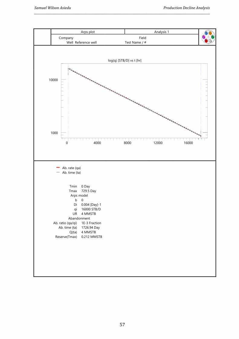
Samuel Wilson Asiedu Production Decline Analysis ______________________________________________________________________________________________________________________
57
Arps plot Analysis 1 Company
Well
Reference
well
Field
Test Name / #
log(q) [STB/D] vs t [hr]
10000
1000
0 4000 8000 12000 16000
Ab. rate (qa)
Ab. time (ta)
Tmin 0 Day
Tmax 729.5 Day
Arps model
b 0
Di 0.004 [Day]-1
qi 16000 STB/D
UR 4 MMSTB
Abandonment
Ab. ratio (qa/qi) 1E-3 Fraction
Ab. time (ta) 1726.94 Day
Q(ta) 4 MMSTB
Reserve(Tmax) 0.212 MMSTB
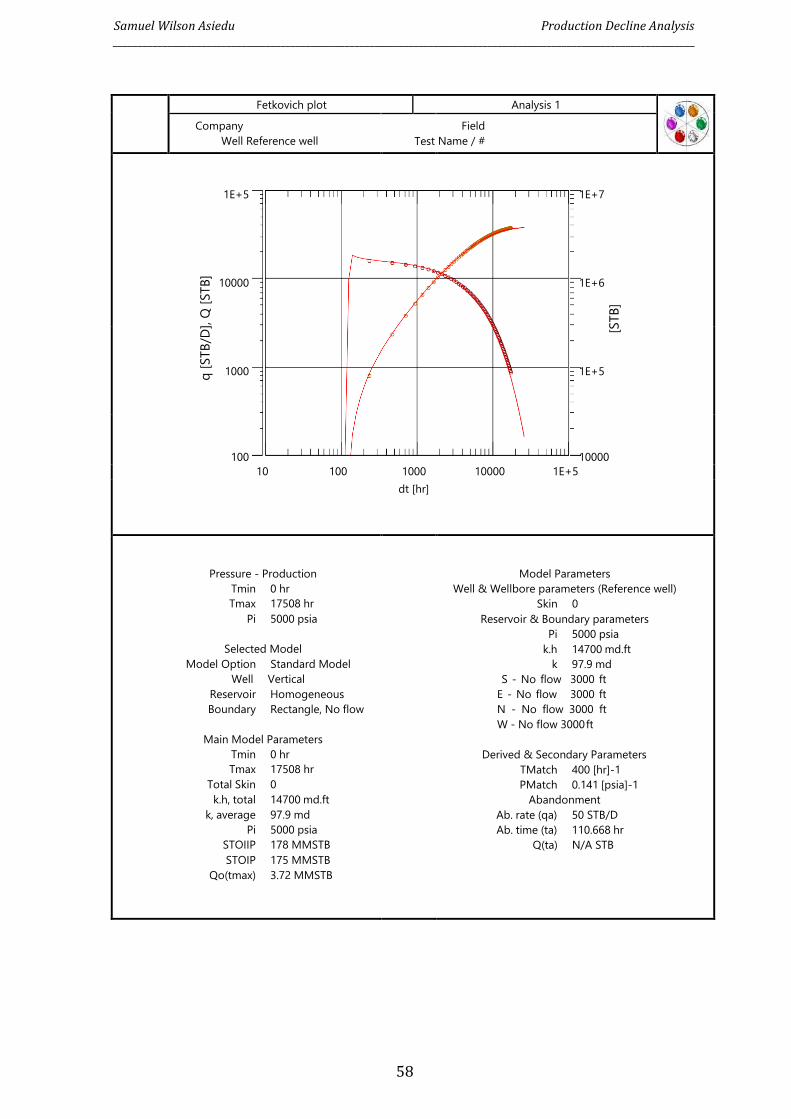
Samuel Wilson Asiedu Production Decline Analysis ______________________________________________________________________________________________________________________
58
q [
STB
/D], Q
[STB
]
[STB
]
Fetkovich plot Analysis 1
Company
Well Reference well
Test
Field
Name / #
1E+5
1E+7
10000
1E+6
1000
1E+5
100
10000
10 100 1000 10000 1E+5
dt [hr]
Pressure - Production
Tmin 0 hr
Tmax 17508 hr
Pi 5000 psia
Selected Model
Model Option Standard Model
Well Vertical
Reservoir Homogeneous
Boundary Rectangle, No flow
Main Model Parameters
Tmin 0 hr
Tmax 17508 hr
Total Skin 0
k.h, total 14700 md.ft
k, average 97.9 md
Pi 5000 psia
STOIIP 178 MMSTB
STOIP 175 MMSTB
Qo(tmax) 3.72 MMSTB
Model Parameters
Well & Wellbore parameters (Reference well)
Skin 0
Reservoir & Boundary parameters
Pi 5000 psia
k.h 14700 md.ft
k 97.9 md
S - No flow 3000 ft
E - No flow 3000 ft
N - No flow 3000 ft
W - No flow 3000 ft
Derived & Secondary Parameters
TMatch 400 [hr]-1
PMatch 0.141 [psia]-1
Abandonment
Ab. rate (qa) 50 STB/D
Ab. time (ta) 110.668 hr
Q(ta) N/A STB
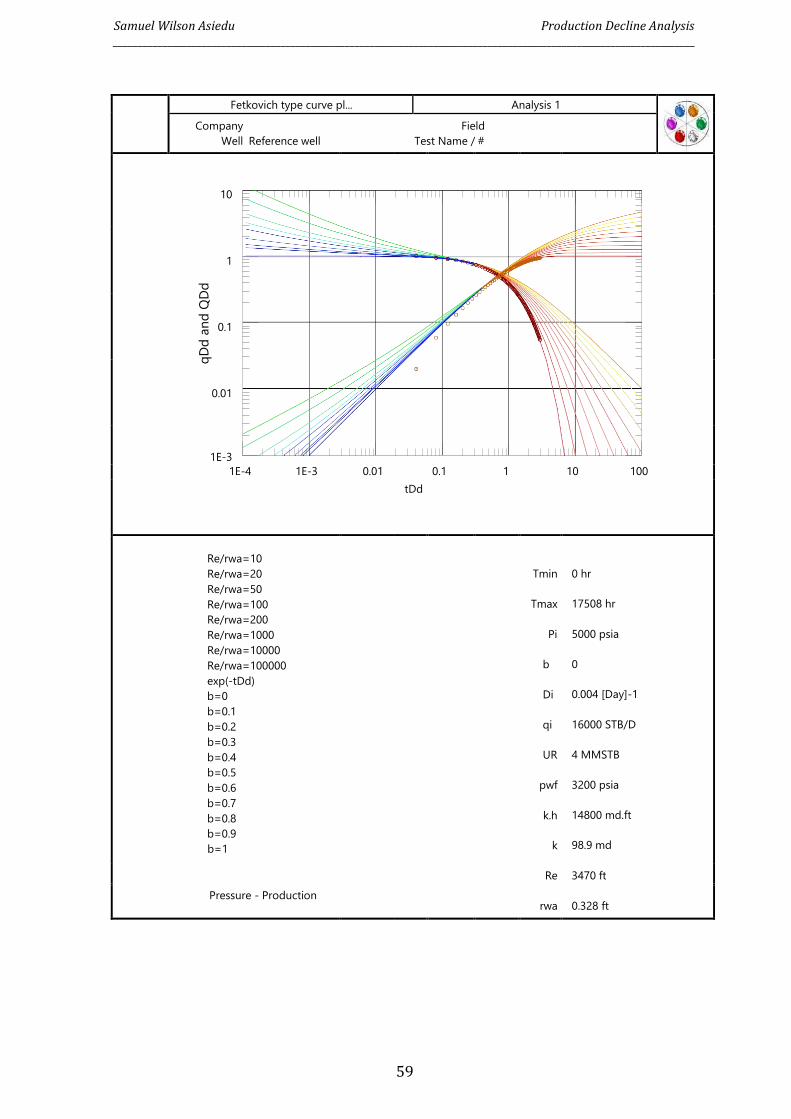
Samuel Wilson Asiedu Production Decline Analysis ______________________________________________________________________________________________________________________
59
qD
d a
nd
QD
d
Fetkovich type curve pl... Analysis 1
Company Field
Well Reference well Test Name / #
10
1
0.1
0.01
1E-3
1E-4 1E-3 0.01 0.1 1 10 100
tDd
Re/rwa=10
Re/rwa=20
Re/rwa=50
Re/rwa=100
Re/rwa=200
Re/rwa=1000
Re/rwa=10000
Re/rwa=100000
exp(-tDd)
b=0
b=0.1
b=0.2
b=0.3
b=0.4
b=0.5
b=0.6
b=0.7
b=0.8
b=0.9
b=1
Tmin
Tmax
Pi
b
Di
qi
UR
pwf
k.h
k
0 hr
17508 hr
5000 psia
0
0.004 [Day]-1
16000 STB/D
4 MMSTB
3200 psia
14800 md.ft
98.9 md
Re 3470 ft
Pressure - Production rwa 0.328 ft
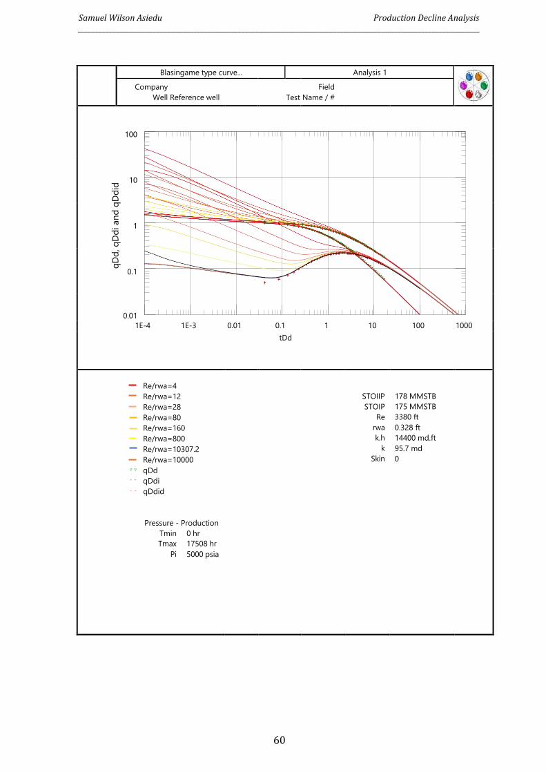
Samuel Wilson Asiedu Production Decline Analysis ______________________________________________________________________________________________________________________
60
qD
d, q
Dd
i an
d q
Dd
id
Blasingame type curve... Analysis 1
Company
Well Reference well
Test
Field
Name / #
100
10
1
0.1
0.01
1E-4 1E-3 0.01 0.1 1 10 100 1000
tDd
Re/rwa=4
Re/rwa=12
Re/rwa=28
Re/rwa=80
Re/rwa=160
Re/rwa=800
Re/rwa=10307.2
Re/rwa=10000
qDd
qDdi
qDdid
Pressure - Production
Tmin 0 hr
Tmax 17508 hr
Pi 5000 psia
STOIIP
STOIP
Re
rwa
k.h
k
Skin
178 MMSTB
175 MMSTB
3380 ft
0.328 ft
14400 md.ft
95.7 md
0
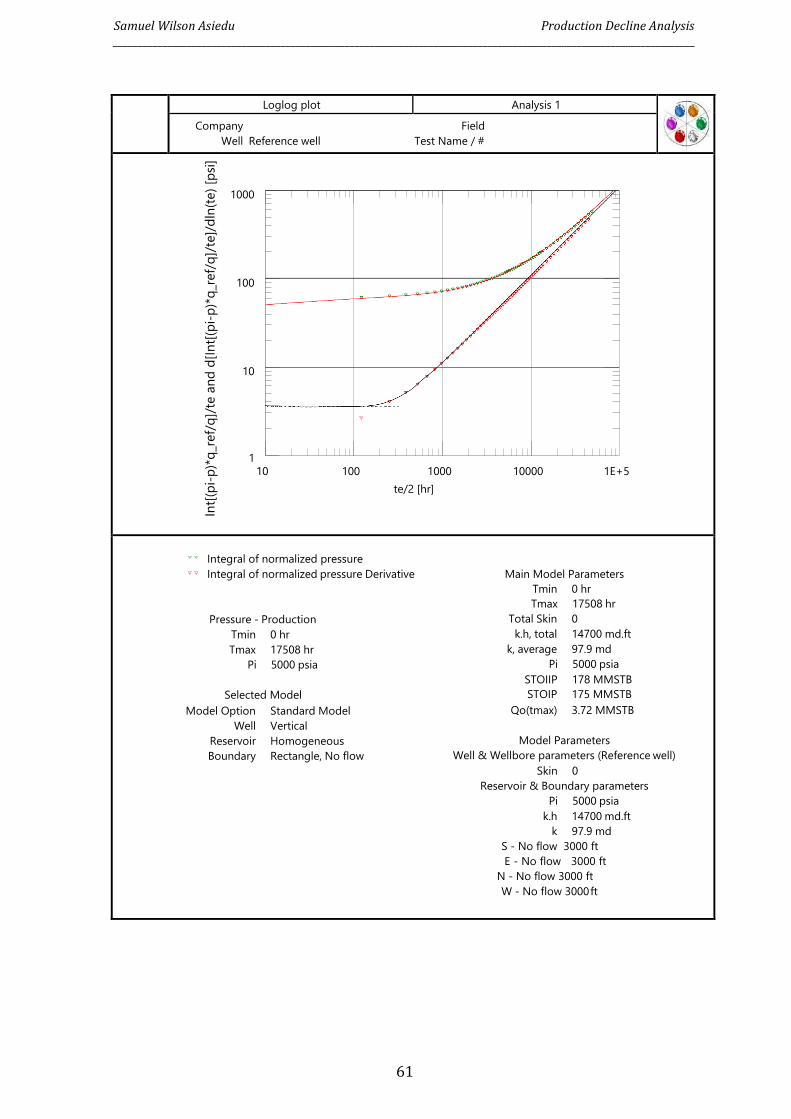
Samuel Wilson Asiedu Production Decline Analysis ______________________________________________________________________________________________________________________
61
Int[
(pi-
p)*
q_r
ef/
q]/
te a
nd
d[I
nt[
(pi-
p)*
q_r
ef/
q]/
te]/
dln
(te)
[psi
]
Loglog plot Analysis 1
Company Field
Well Reference well Test Name / #
1000
100
10
1 10 100 1000 10000 1E+5
te/2 [hr]
Integral of normalized pressure
Integral of normalized pressure Derivative Main Model Parameters
Tmin 0 hr
Tmax 17508 hr
Pressure - Production Total Skin 0
Tmin 0 hr k.h, total 14700 md.ft
Tmax 17508 hr k, average 97.9 md
Pi 5000 psia Pi 5000 psia
STOIIP 178 MMSTB
Selected Model STOIP 175 MMSTB
Model Option Standard Model Qo(tmax) 3.72 MMSTB
Well Vertical
Reservoir Homogeneous Model Parameters
Boundary Rectangle, No flow Well & Wellbore parameters (Reference well)
Skin 0
Reservoir & Boundary parameters
Pi 5000 psia
k.h 14700 md.ft
k 97.9 md
S - No flow 3000 ft
E - No flow 3000 ft
N - No flow 3000 ft
W - No flow 3000 ft
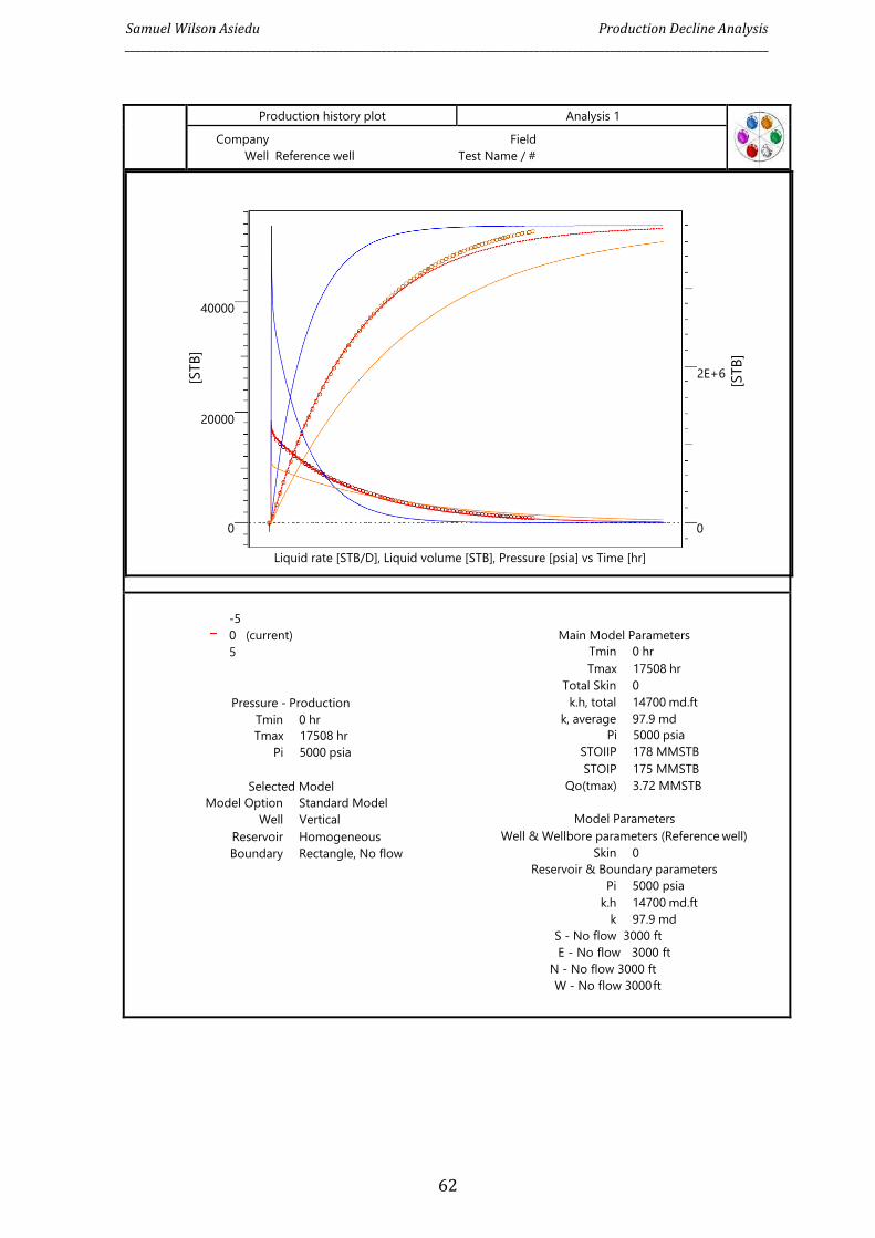
Samuel Wilson Asiedu Production Decline Analysis ______________________________________________________________________________________________________________________
62
[STB
]
[STB
]
Production history plot Analysis 1
Company Field
Well Reference well Test Name / #
40000
2E+6
20000
0 0
Liquid rate [STB/D], Liquid volume [STB], Pressure [psia] vs Time [hr]
-5
0 (current) Main Model Parameters
5 Tmin 0 hr
Tmax 17508 hr
Total Skin 0
Pressure - Production k.h, total 14700 md.ft
Tmin 0 hr k, average 97.9 md
Tmax 17508 hr Pi 5000 psia
Pi 5000 psia STOIIP 178 MMSTB
STOIP 175 MMSTB
Selected Model Qo(tmax) 3.72 MMSTB
Model Option Standard Model
Well Vertical Model Parameters
Reservoir Homogeneous Well & Wellbore parameters (Reference well)
Boundary Rectangle, No flow Skin 0
Reservoir & Boundary parameters
Pi 5000 psia
k.h 14700 md.ft
k 97.9 md
S - No flow 3000 ft
E - No flow 3000 ft
N - No flow 3000 ft
W - No flow 3000 ft
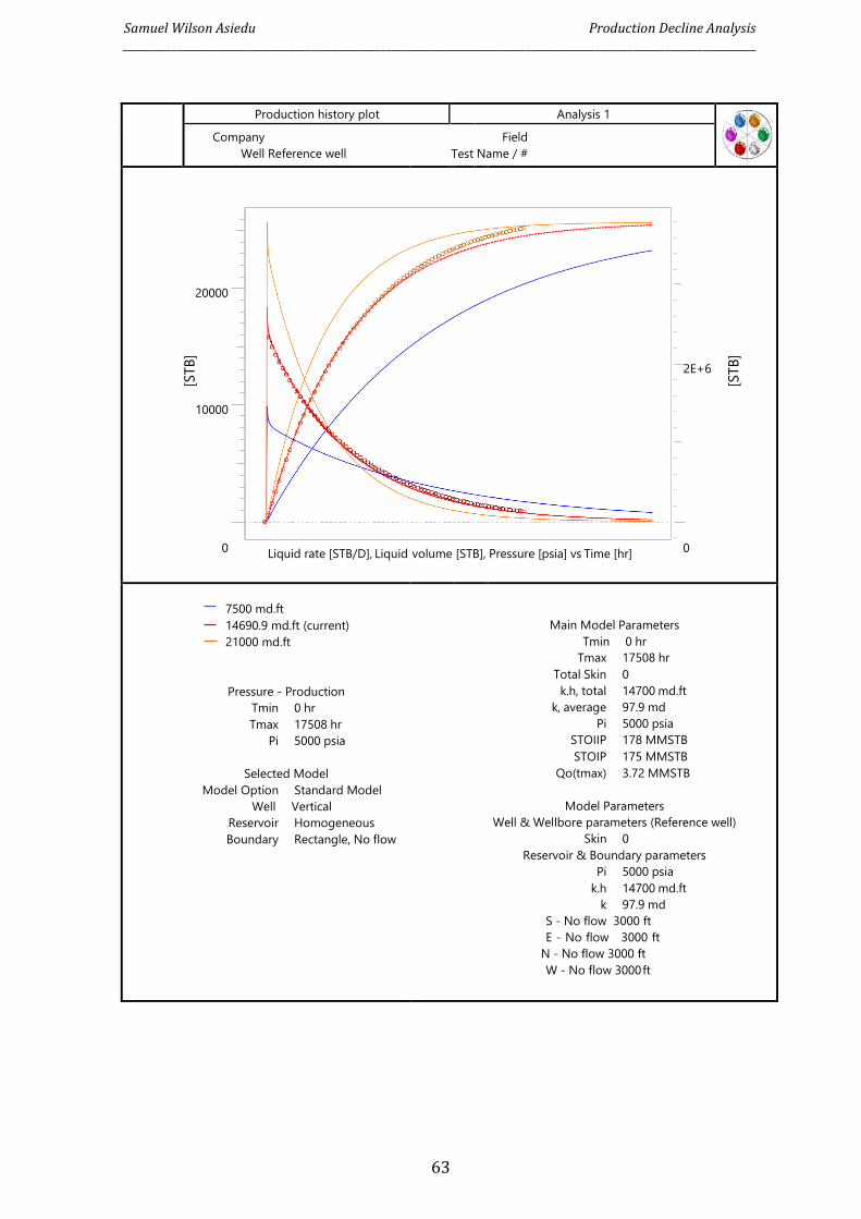
Samuel Wilson Asiedu Production Decline Analysis ______________________________________________________________________________________________________________________
63
[STB
]
[STB
]
Production history plot Analysis 1
Company
Well Reference well
Test
Field
Name / #
20000
10000
0 Liquid rate [STB/D], Liquid
volume
[STB],
2E+6
Pressure [psia] vs Time [hr] 0
7500 md.ft
14690.9 md.ft (current)
21000 md.ft
Pressure - Production
Tmin 0 hr
Tmax 17508 hr
Pi 5000 psia
Selected Model
Model Option Standard Model
Well Vertical
Reservoir Homogeneous
Boundary Rectangle, No flow
Main Model Parameters
Tmin 0 hr
Tmax 17508 hr
Total Skin 0
k.h, total 14700 md.ft
k, average 97.9 md
Pi 5000 psia
STOIIP 178 MMSTB
STOIP 175 MMSTB
Qo(tmax) 3.72 MMSTB
Model Parameters
Well & Wellbore parameters (Reference well)
Skin 0
Reservoir & Boundary parameters
Pi 5000 psia
k.h 14700 md.ft
k 97.9 md
S - No flow 3000 ft
E - No flow 3000 ft
N - No flow 3000 ft
W - No flow 3000 ft
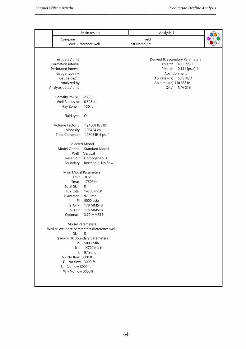
Samuel Wilson Asiedu Production Decline Analysis ______________________________________________________________________________________________________________________
64
Main results Analysis 1
Company Field
Well Reference well Test Name / #
Test date / time Derived & Secondary Parameters
Formation interval TMatch 400 [hr]-1
Perforated interval PMatch 0.141 [psia]-1
Gauge type / # Abandonment
Gauge depth Ab. rate (qa) 50 STB/D
Analyzed by Ab. time (ta) 110.668 hr
Analysis date / time Q(ta) N/A STB
Porosity Phi (%) 23.2
Well Radius rw 0.328 ft
Pay Zone h 150 ft
Fluid type Oil
Volume Factor B 1.24868 B/STB
Viscosity 1.08424 cp
Total Compr. ct 1.18085E-5 psi-1
Selected Model
Model Option Standard Model
Well Vertical
Reservoir Homogeneous
Boundary Rectangle, No flow
Main Model Parameters
Tmin 0 hr
Tmax 17508 hr
Total Skin 0
k.h, total 14700 md.ft
k, average 97.9 md
Pi 5000 psia
STOIIP 178 MMSTB
STOIP 175 MMSTB
Qo(tmax) 3.72 MMSTB
Model Parameters
Well & Wellbore parameters (Reference well)
Skin 0
Reservoir & Boundary parameters
Pi 5000 psia
k.h 14700 md.ft
k 97.9 md
S - No flow 3000 ft
E - No flow 3000 ft
N - No flow 3000 ft
W - No flow 3000 ft

![Prediction of Reservoir Performance Applying Decline Curve ... · Decline curve analysis is the most currently method used available and sufficient [1].The most popular decline curve](https://static.fdocuments.in/doc/165x107/5eb99c14e247933c8377a1f7/prediction-of-reservoir-performance-applying-decline-curve-decline-curve-analysis.jpg)