Product Quality, Linder, and the Direction of Trade

Juan Carlos Hallak∗

University of Michigan

June 2004

Abstract

A substantial amount of theoretical work predicts that quality plays an important role as a

determinant of the global patterns of bilateral trade. This paper develops an empirical frame-

work to estimate the empirical relevance of this prediction. In particular, it identifies the effect

of quality operating on the demand side through the relationship between per capita income and

aggregate demand for quality. The model yields predictions for bilateral flows at the sectoral

level, and is estimated using cross-sectional data for bilateral trade among 60 countries in 1995.

The empirical results confirm the theoretical prediction: rich countries tend to import relatively

more from countries that produce high quality goods. The paper also shows that a severe ag-

gregation bias explains the failure of the literature so far to find consistent empirical support for

the “Linder hypothesis”, the conjectured corollary to the first theory relating product quality

and the direction of trade.

∗Department of Economics, 351C Lorch Hall, Ann Arbor, MI 48109. e-mail: hallak@umich.edu. I am particularly

grateful to Elhanan Helpman and Marc Melitz for their guidance and support, to Alan Deardorff for very helpful

discussions and comments, and to Peter Morrow for excellent research assistance. I also thank Robert Barro, Francesco

Caselli, Edwin Diewert, Doireann Fitzgerald, Daniel Hamermesh, Jim Levinsohn, Rosa Matzkin, Gary Solon, Silvana

Tenreyro, and seminar participants at Columbia, Di Tella, Duke, Harvard, Michigan, Michigan State, Purdue, San

Andres, Texas-Austin, Toronto, University of British Columbia, the World Bank, Yale, and the EIIT Conference for

helpful comments and suggestions.

1

1 Introduction

Increasing evidence indicates that there are large differences across countries in the quality of the

products that they produce and export. While traditional theories of international trade neglect

the existence of product quality differences across countries, a substantial amount of theoretical

work predicts that quality systematically affects the direction of international trade. In spite of the

theoretical predictions, there is yet no evidence evaluating the empirical relevance of quality as a

determinant of bilateral trade volumes. Understanding the influence of quality on the direction of

trade might be crucial for enhancing the predictive power of benchmark empirical trade models,

which will result in improved assessments of the impact of other determinants of trade, such as

commercial policies or natural barriers to international exchange.

Linder (1961) first noted the role of quality as a determinant of the direction of trade. He

argued that richer countries spend a larger proportion of their income on high quality goods.

He also argued that closeness to demand is a source of comparative advantage, providing richer

countries with a comparative advantage in the production of high quality goods–the goods that

they demand. He then conjectured that the congruence of production and consumption patterns

leads countries with similar income per capita to trade more with one another. This is the Linder

hypothesis, the earliest theory explaining the effects of quality differences on the direction of trade.

It has received considerable attention for its contrast with the standard Heckscher-Ohlin theory,

which predicts trade intensity to be higher between countries of dissimilar income per capita–as

the latter reflects differences in relative factor endowments.

More recent theoretical work has developed general equilibrium models to formalize the role of

quality as a determinant of trade patterns.1 These models share two key features with Linder’s

theory. First, rich countries have a comparative advantage in the production of high quality goods

(comparative advantage comes here from productivity or factor endowment differences). Second,

rich countries consume high quality goods in larger proportions than poorer countries. Even though

the models yield theoretical results in the spirit of the Linder hypothesis, they do not obtain this

conjecture as a general result.

Recent empirical work provides support for the supply-side relationship between per capita in-

come and quality production postulated by Linder and subsequent theorists. Schott (2004) shows

1See Falvey and Kierzkowski (1987), Flam and Helpman (1987), Stokey (1991), Murphy and Shleifer (1997).

2

that export unit values increase systematically with exporter per capita income and relative fac-

tor endowments, while Hummels and Klenow (2002) use quantities exported and proxies for the

number of varieties to argue that quality differences are necessary to explain (at least part of) the

observed differences in unit values. In contrast to the evidence on the supply side, the demand-side

relationship between per capita income and quality consumption, and the impact of this relation-

ship on bilateral trade flows, have not been the subject of similar empirical scrutiny. In particular,

there is yet no attempt at estimating the existence and magnitude of such a quality-driven demand

effect on the global patterns of bilateral trade.2

A vast related literature has concentrated on estimating the Linder hypothesis. Since this is a

conjectured corollary to a theory that places quality at center stage, tests of this hypothesis could be

interpreted as evidence on the role of quality. This literature typically uses the gravity equation as

benchmark3, and adds a “Linder term”, a measure of income dissimilarity between pairs of countries.

The Linder hypothesis predicts a negative sign for the estimated coefficient on the Linder term.

But the empirical results on the sign of this coefficient are mixed.4 There is nevertheless an even

more fundamental problem than failure to confirm the Linder hypothesis: the empirical framework

used by this literature cannot properly identify the role of quality as a determinant of the direction

of trade. First, the prediction that the intensity of trade is higher between countries with similar

income per capita can also result from inter-sectoral non-homotheticities in demand, not related

to quality. This is the case if income elasticities differ across sectors, and richer countries have a

comparative advantage in sectors with high income elasticities.5 Second, quality effects coexist with

other traditional (inter-sectoral) determinants of trade, such as differences in factor proportions.

But the gravity-equation framework does not nest these different forces. It is thus unable to isolate

the role of quality from other inter-sectoral determinants of trade.

This paper provides a testable framework to estimate the impact of quality on the direction

2Brooks (2003) provides evidence of this effect in a specific context. She shows that differences in export shares

among Colombian firms (in industries with exports largely oriented to the US) depend negatively on the industry-level

quality gap relative to G7 countries, as measured by differences in unit value of exports to the US.3The gravity equation, in its traditional form, postulates a log-linear relationship between the volume of bilateral

trade, the GDP of each country, and the distance between them.4See surveys in Deardorff (1984), Leamer and Levinsohn (1995), and McPherson, Redfearn, and Tieslau (2001).5The role of this type of non-homotheticities has been addressed by Markusen (1986), Hunter and Markusen

(1988), Bergstrand (1989), Hunter (1991), Deardorff (1998), and Matsuyama (2000).

3

of trade. In particular, it identifies the effect of quality operating on the demand side through

the relationship between income and aggregate demand for quality. The theoretical framework,

described in section 2, yields an empirical specification for estimating bilateral trade that has a

strong resemblance to the gravity equation. However, it yields predictions for bilateral trade flows

at the sectoral instead of at the aggregate level. By focusing on sectoral trade, the empirical

specification embeds and controls for inter-sectoral determinants of comparative advantage. A

parameter in the demand system captures the extent to which income per capita affects quality

choice. In the empirical specification, this parameter translates into the coefficient on an interaction

term between the exporter quality and the importer per capita income. If income affects quality

demand–and therefore trade patterns–this coefficient is predicted to be positive.

Quality is unobservable. I follow two complementary approaches to deal with unobserved qual-

ity. First, based on recent empirical findings, in section 3 I use exporter income per capita as a

proxy for quality. The relevant term in the empirical specification then becomes the interaction

between exporter and importer per capita incomes, capturing respectively supply of and demand

for quality. I estimate the empirical model using a cross-section of sectoral bilateral trade flows (at

the 3-digit level) among 60 countries in 1995. Sectors are divided into three categories according

to Rauch (1999): Differentiated, Reference-priced, and Homogeneous. The theory is primarily ap-

plicable to Differentiated sectors. In those sectors, the results support the theoretical prediction:

rich countries tend to import relatively more from other rich countries–those that produce higher

quality goods. I also estimate the empirical model for sectors in the other two categories to check

that it is indeed quality that drives the results. In Reference-priced sectors, where the theory may

still reasonably apply, the results are similar to those obtained for Differentiated sectors. In Homo-

geneous sectors, however, the theory is not expected to apply, as the income interaction term no

longer captures supply of and demand for quality. Consistent with this prediction, the results are

very different here; the interaction term shows no systematic effect on trade.

Since the interaction term is very similar to a Linder term, the results can be interpreted as a

sector-level confirmation of the Linder hypothesis. Furthermore, they are not sensitive to the use

of alternative Linder terms often used in the literature. But when the empirical specification is

estimated on aggregate trade flows–as is typically done–the results are reversed. I show that this

is the result of an aggregation bias, the direction of which depends on the extent of cross-country

4

correlation between per capita income and sectoral pattern of specialization. The aggregation bias

explains the failure of the literature so far to find consistent evidence in support of the Linder

hypothesis. If quality drives its main insight–as originally conjectured by Linder–this suggests

a reformulation of the hypothesis as a sector-level prediction, requiring inter-sectoral determinants

of trade to be controlled for.

Keeping constant factors such as production costs, we expect higher quality goods to command

higher prices. Export prices then convey useful information on product quality. In section 4, I

construct export price indices at the sectoral level from unit values of exports to the US (calculated

at the finest possible level of aggregation). I then use these indices as indicators of quality. The

advantage of this approach, relative to the approach in the previous section, is the use of cross-

sector variation in export price indices within countries to capture cross-sector variation in quality

levels. The disadvantage is that measurement error is pervasive in the dataset used to construct the

indices. The findings here are still consistent with the theoretical prediction: rich countries tend

to import relatively more from countries that produce higher quality goods. These results further

support the findings in the previous section on the role of quality as a determinant of trade. They

also provide complementary evidence that it is quality–as opposed to other factors correlated with

income per capita but unrelated to quality– that drives those results. Section 5 concludes.

2 Theoretical Framework

2.1 The Demand System

Demand in each country k is generated by a representative consumer with a two-tier utility function.

The upper tier utility is weakly separable into subutility indices defined for each differentiated-good

sector z = 1, ..., Z, and for each homogeneous-good sector g = Z + 1, ...,G,

Uk = Uhuk1, ..., u

kz , ..., u

kZ , u

kZ+1, ..., u

kg , ..., u

kG

i. (1)

The subutility index ukg is a general function of the quantity consumed of good g. The subutility

index ukz takes the specific form:

ukz =

⎡⎣Xh∈Hz

³θγkzh qh

´αz⎤⎦ 1αz

0 < αz, γkz < 1 ∀z, k (2)

5

where ukz is defined over all varieties h ∈ Hz in sector z. In (2), qh and θh are the quantity and

quality of variety h, and the parameter γkz is the intensity of preference for quality of country k.

None of the parameters is restricted to be the same across sectors.

The subutility functions ukz are an augmented version of the Dixit-Stiglitz structure of pref-

erences. Quality enters as a utility shifter, while there is still a horizontal dimension of product

differentiation (consumers love variety). This specification of utility is designed to capture differ-

ences across countries in quality demand, stemming from their differences in income. For a given

shape of the income distribution, we expect countries with higher average income to consume a

larger proportion of high-quality goods. In the demand system that this utility generates, the pa-

rameter γk captures–in a reduced form–the effect of income on quality demand at the aggregate

level.

The representative consumer uses two-stage budgeting. In the first stage, for a given expenditure

allocation across sectors Ek1 , ..., E

kZ , ..., E

kG, expenditure on variety h in sector z is:

pkhqkh =

µpkh

θγkzh

¶1−σzP

r∈Hz

µpkr

θγkzr

¶1−σz Ekz = sk(h)Ek

z , (3)

where σz = 1/(1 − αz) > 1 is the elasticity of substitution, and pkh is the price of h faced by

consumers in country k. Equation (3) shows expenditure on h as a share sk(h) of total expenditure

in sector z. This share depends on the value of γk, and it changes with this parameter according

to:

∂sk(h)

∂γkz= λkhz

"ln θh −

Xr∈Hz

s(r) ln θr

#, λkhz=

µpkh

θγkzh

¶1−σz(σz − 1)

Pr∈Hz

µpkr

θγkzr

¶1−σz > 0. (4)

Equation (4) highlights the main characteristic of the demand system. For a variety h of above-

average quality–the term in brackets in (4) is positive–a higher γk induces a larger share spent

on h. For a variety h of below-average quality, a higher γk induces a smaller share spent on h.

Countries with higher γk thus spend a larger share of their income on high quality goods. Allowing

γk to vary across countries, this demand system has the convenient property of accommodating

in a simple form cross-country differences in the pattern of expenditures for goods of different

6

quality.6 A special case arises when γk is the same for every country. In that case, the demand

system is equivalent to the demand system generated by the Dixit-Stiglitz structure of preferences,

where there are no differences across countries in quality choice.7 Since Dixit-Stiglitz preferences

are standard in international trade models and empirical frameworks with product differentiation,

the proposed demand system has the additional advantage of embedding a meaningful benchmark

against which to assess the impact of quality on aggregate demand and trade.

2.2 Bilateral trade flows at the sectoral level

Country i produces Niz different varieties in sector z. These varieties are symmetric; they share the

same quality and sell at the same price.8 We can multiply equation (3) by the number of varieties

Niz to obtain country k’s total imports from i in sector z:

impkiz = Niz

µpizτkiz

θγkziz

¶1−σzP

r∈Hz

µprτkr

θγkzr

¶1−σz Ekz , (5)

where we use pkiz = pizτkiz, the equality between import price and the product of export price and

trade cost factor between i and k.

Countries differ in the quality of the goods they produce and in their pattern of sectoral spe-

cialization. Recent empirical work [Schott (2004), Hummels and Klenow (2002)] provides evidence

characterizing supply-side determinants of quality production. This paper instead takes the distrib-

ution of quality production across countries as given and, conditional on this distribution, attempts

to identify the effect of quality on the direction of trade operating on the demand side through the

relationship between income and quality choice. Income as a determinant of the demand for prod-

uct quality–and hence of the intensity of trade between country pairs–has been one the main

ingredients of most theoretical work addressing the impact of quality on the direction of trade.

6 I do not address here the effects of differences in higher moments of the income distribution. See Francois and

Kaplan (1996) and Dalgin, Mitra, and Trindade (2004) for an empirical treatment of inequality and trade based on

inter-sectoral non-homotheticities.7 In this case, quantity substitutes for quality at the same rate in every country. Quantities and prices can then

be renormalized to "common-quality" units to obtain the typical Dixit-Stiglitz specification.8This will not be a strong restriction so long as the variation of quality levels within countries is small compared

to the variation of quality levels between countries.

7

However, there is yet no empirical evidence identifying this effect in global patterns of trade.

The proposed demand system allows quality choice to depend on a country-specific parameter.

In the special case with equal γk across countries, the demand system is equivalent to the standard

Dixit-Stiglitz structure of preferences, which does not allow the demand for quality to vary across

countries. I show next that Dixit-Stiglitz preferences impose a strong restriction on the relationship

between bilateral flows at the sectoral level. This restriction is independent of the distribution of

quality production across countries, and thus provides a key for identifying quality effects on the

direction of trade.

Using (5), consider US (country k) imports of Rubber Tires (sector z) from Germany (country

i). Consider also US imports of tires from Turkey (country j) by replacing i with j in (5). The ratio

between these two expressions indicates the ratio of US imports of tires from Germany relative to

those originating from Turkey, and is independent of the expenditure level and the price index for

tires in the US:

ratiokij(z) =Niz

Njz

⎛⎝ pizτkiz/θ

γkziz

pjzτkjz/θγkzjz

⎞⎠1−σz . (6)

Replacing k with l in (6), consider the same ratio for a different importer, Argentina (country

l). Then, compare these two ratios by taking the ratio between the two:

rklij (z) =ratiokij(z)

ratiolij(z)=

Ãτkiz/τ

kjz

τ liz/τljz

!1−σz "(θiz/θjz)

γkz

(θiz/θjz)γlz

#σz−1. (7)

To abstract from the impact of trade costs, assume for now thatτkiz/τ

kjz

τ liz/τljz= 1. Then,

rklij (z) =

"(θiz/θjz)

γkz

(θiz/θjz)γlz

#σz−1. (8)

There are three possible cases in (8). The first one is trivial. If Germany and Turkey produce

the same quality of tires (θi = θj), then relative imports from Germany and Turkey are the

same for both the US and Argentina (rklij = 1). A much more relevant case is the second one,

which is our benchmark case of no income effects on quality choice. If the US and Argentina

have the same intensity of preference for quality (γk = γl), then relative imports from Germany

and Turkey will still be the same for both importers (rklij = 1), even if qualities are different

(θi 6= θj). As argued before, standard Dixit-Stiglitz preferences can accommodate this case after an

8

appropriate normalization to “common-quality” units. Thus interpreted, these preferences impose

the restriction that any two countries’ relative imports from any other two countries are identical,

i.e. rklij = 1, regardless of the quality produced by the two exporting countries.9 The restriction

does not neglect inter-sectoral determinants of trade. Suppose that Germany has a comparative

advantage in producing tires. Then, Germany will have many firms in this sector. Niz will be large,

and Germany will be a large exporter of tires.10 But exports from Germany will be large to both

the US and Argentina without affecting rklij . A similar exercise focusing on an importer provides the

same answer. Suppose that Argentina has a comparative advantage in producing tires. We then

expect a large number of firms there, leading to a low price index for tires since domestic goods do

not pay trade costs. Relative prices of imported varieties will then be high, discouraging Argentina’s

imports from both Germany and Turkey. But again, rklij will not be affected. Finally, suppose that

Ekz is large for the US because of a combination of size and inter-sectoral non-homotheticities in

demand. This will affect US imports from both countries proportionally, but it will still not affect

the relative ratio rklij .

It is only in the third case, where both quality and the intensity of preference for quality are

different (θi 6= θj and γk 6= γl), that rklij 6= 1. Only then will quality affect the relative intensity of

sectoral trade between different country pairs. If Germany’s quality is higher (θi > θj) and US’s

intensity of preference for quality is higher (γk > γl), then the US will import relatively more from

Germany while Argentina will import relatively more from Turkey. More generally, countries with

higher γk will import relatively more from countries that produce higher quality goods.

Taking logarithms on both sides of equation (5), we obtain the following prediction for bilateral

trade:

ln impkiz = lnNiz − eσz ln piz − ln Xr∈Hz

Ãpkr

θγkzr

!−eσz+ lnEk

z − eσz ln τkiz + eσzγkz ln θiz, (9)

where eσz = σz − 1. In a cross-section of bilateral trade flows, the first two terms on the RHS

are specific to exporting country i. These terms take the same value when i is the exporter,

independent of who importer k is. In the econometric specification, they will be captured by

exporter fixed effects. Similarly, the next two terms are specific to importer k and take the same9In the more general case, this is only true after controlling for differences in bilateral trade costs.10Romalis (2004) derives the effect of comparative advantage on the number of firms in a Heckscher-Ohlin model

that accounts for product differentiation and trade costs.

9

value independent of exporter i. These terms will be captured by importer fixed effects. Only the

last two terms are specific to the bilateral pair. I assume that trade costs are determined by:

ln τkiz = ηz lnDistki +eβzI

ki − vkiz, (10)

where Distki is the bilateral distance between each country pair, vkiz is a random disturbance, andeβz is a vector of parameters associated with dummy variables I

ki indicating whether the country

pair shares, respectively, a common border, a common language, a preferential trade agreement, a

colonial relationship, or a common colonizer.11 I also postulate a relationship between the intensity

of demand for quality–captured by γkz–and income12:

γkz = γz + µz ln yk. (11)

Under the null hypothesis that income does not affect aggregate demand for quality, µz = 0, and

γkz = γz. This is the benchmark Dixit-Stiglitz case. Under the alternative hypothesis that it does

affect aggregate demand for quality, µz > 0, and γkz increases with income.

Combining (10) and (11) with (9), we obtain:

ln impkiz = ϕiz + ψkz − eσzηz lnDistki + βzI

ki + eσzµz ln θiz ln yk + eσzvkiz, (12)

where ϕiz and ψkz are fixed effects for exporter and importer country, respectively, and βz = −eσzeβz.

I am unable to estimate (12) because I do not observe quality (θiz). The next two sections deal

with unobserved quality in two different ways. First, exporter income is used as a proxy for quality.

Second, export price indices (constructed from export unit values) are used as indicators of quality.

3 Exporter Income as Proxy for Quality

There is increasing evidence that suggests the existence of a positive relationship between per capita

income and quality supply. Different trade theories are consistent with this evidence. For example,

a Ricardian view of quality specialization would predict that richer countries will produce higher

11The empirical specification would not change if trade costs depended on quality, so long as they are modeled

with a (negative) function of quality as an additive term in (10). This term would be subsumed into the exporter

fixed effect.12Throughout the paper–unless explicitly noted–income will refer to income per capita.

10

quality goods if they have a relatively larger productivity advantage in the production of those

goods. Alternatively, a factor proportions view of quality specialization would predict that richer

countries, which tend to be capital abundant, will have a comparative advantage in the production

of high quality goods if these goods are capital intensive.13 Based on the evidence of a positive

relationship between quality supply and income, but without taking a stand on which underlying

theory generates this relationship, I postulate the following stochastic log-linear equation:

ln θiz = δz ln yi + ηiz. (13)

The random disturbance ηiz introduces quality variation between sectors for a given country, al-

lowing the cross-country ordering of sectoral quality levels to differ from the ordering of income.

Substituting (13) into (12), we obtain:

ln impkiz = ϕiz + ψkz − eσzηz lnDistki + βzI

ki + eσzµzδz ln yi ln yk + εkiz, (14)

where εkiz = eσzµzηiz+eσzvkiz.14 The component disturbances ηiz and vkiz are assumed to be uncorre-lated with the regressors; therefore, so is εkiz. I will estimate (14) on a cross-section of bilateral trade

flows at the sectoral level. Unfortunately, I will not be able to separately identify the magnitude of

µz. But since eσz > 0, if based on the available evidence we maintain the assumption that δz > 0,

then a test of the joint hypothesis eσzµzδz = 0 will imply a test of the hypothesis µz = 0.Several sectors used in the estimation contain intermediate goods. If we interpret (1) and (2)

as a production function of a final good based on the use of intermediate inputs, then (3) is the

demand function for these inputs. In that case, it may be reasonable to assume that γkz is not a

function of the importer income as in (11), but of the quality of the final good θkz (assuming that

it is demanded in only one sector). Since the quality of the final good is in turn a function of the

importer income by (13), we can still derive (14). The error term contains additional terms in this

case, but it is still uncorrelated with the regressors.

Equation (14) is a prediction for bilateral trade at the sectoral level. Estimating it with aggregate

data would only be appropriate if the parameters were constrained to be equal across sectors. This

restriction is not plausible in general. In particular, it will be strongly violated in the case of the

exporter and importer fixed effects, which must be sector-specific as they control for inter-sectoral13Schott (2004) provides empirical evidence in support of this view.14A constant in (13) would be absorbed in the fixed effect ψkz , without affecting (14).

11

determinants of comparative advantage. I thus estimate (14) sector by sector. Also, to obtain a

single estimate of the parameter of interest, I estimate (14) pooling the observations across sectors.

In this case, I allow all the parameters to take sector-specific values except for the cross-sector

restriction eσzµzδz = eσµδ.Finally, I focus on differentiated-good sectors because the theory underlying (14) is only valid

for those sectors. But I also use other sectors to benchmark the results.

3.1 Data and sample selection

The data consist of a cross section of bilateral trade flows and country-level variables for 60 countries

in 1995. Bilateral trade data, disaggregated at the sectoral level, come from Feenstra (2000). The

dataset is based on the World Trade Analyzer assembled by Statistics Canada. I define sectors at

the 3-digit SITC (Rev.2) level.

I follow Rauch’s (1999) classification of 4-digit SITC sectors into three categories. Homogeneous

sectors include goods that are internationally traded in organized exchanges, with a well-defined

price (e.g., wheat). Reference-priced sectors include goods that are not traded in organized ex-

changes, but have reference prices available in specialized publications (e.g., polyethylene). Differ-

entiated sectors are those sectors that do not satisfy either of the two previous criteria. Rauch uses

two standards to make his classification, one “liberal” and one “conservative”. I use the liberal

standard because it is more stringent in the classification of goods as Differentiated. When a 3-digit

sector includes 4-digit subsectors that belong to different classifications, the 3-digit sector is broken

down accordingly, each part including only the relevant 4-digit sectors.

There is a large proportion of bilateral country pairs with zero trade. The proportion is larger

for smaller countries. Since I want to prevent zero-trade observations from dominating the sample,

I concentrate only on relatively large countries. I include countries with a population larger than 3

million, and with more than 2 billion-dollar imports of Differentiated goods. Hungary is additionally

excluded because sectoral trade data are of poor quality. Algeria, Iran, Libya, and the US are

excluded because they lack data on export unit values, used in the next section of the paper. In

the case of the US, export unit values are not available because they are obtained from a database

on US imports. The final sample consists of 60 countries, listed in Table A1. I also drop very

small sectors, keeping only sectors with a volume of trade (within the 60 selected countries) above

12

2 billion dollars. The final sample includes 114 Differentiated sectors, 51 Reference-priced sectors,

and 38 Homogeneous sectors. They are listed in Tables A2, A3, and A4, respectively.

Distance measures great circle distance between capital cities and was prepared by Howard

Shatz (1997). Dummies for border, common language, colonizer-colony relationship, and common-

colonizer relationship were constructed using the CIA Factbook. Only “official” languages are

considered in the construction of the common language variable. An exception is made for Malaysia-

Singapore, which is recorded as having a common language. Colonial links are only considered if the

colonizer-colony relationship was still in force after 1922. The indicator variable for Preferential

Trade Agreement includes PTAs in force and with substantial coverage in 1995: Andean Pact,

ASEAN, CACM, EFTA, EEA, EU, MERCOSUR, NAFTA, Australia-New Zealand, EC-Turkey,

EFTA-Turkey, EC-Israel, EFTA-Israel. Data on PPP GDP come from the World Bank WDI.

3.2 Estimation results

I first estimate (14) separately for each Differentiated sector using OLS. Since I cannot report de-

tailed regression results for all 114 sectors, I provide summary results for the distribution of the esti-

mated coefficients according to sign and significance levels in Table 1. In all cases, heteroskedasticity-

robust standard errors are used. The results for the coefficient of interest (the interaction term)

are shown in the first row. This coefficient is positive in more than 2/3 of the sectors (78), and

negative in less than 1/3 (36) of the sectors. The coefficient is positive and significant in almost

1/2 of the sectors (56), and negative and significant in 1/5 (23).

The median coefficient across sectors is 0.1218. The interpretation of this coefficient is related

to the ratio of ratios in equations (7) and (8). Keeping trade costs constant, and denoting bµz theestimate of eσzµzδz, we can use (14) to calculate the predicted ratio of ratios:

ln(rklijz) = bµz ln yiyjln

yk

yl. (15)

To understand this expression, take countries at the 75th percentile (Sweden and the UK) and the

25th percentile (Dominican Republican and Lebanon) of the income distribution in our sample.

Consider Dominican Republic’s ratio of imports from the UK relative to those from Lebanon. How

much would this ratio increase if the Dominican Republic were to have the income of Sweden?

Substituting for the actual income values in (15), we obtain: rklijz = exp(0.1218∗1.6115∗ .1.5912) =

13

1.366; Dominican Republic’s imports from the UK relative to Lebanon would increase by 36.6% (in

the median sector). This is the relevant exercise for interpreting the estimated magnitude of the

quality effect. Other typical measures of explanatory power such as the beta coefficient are very

small because size (captured by the dummy variables) and distance dominate most of the variation

in bilateral trade flows.

The last column of Table 1 shows results for the pooled regression, where the coefficient on the

interaction term is constrained to be the same across sectors. Here, as in every pooled regression,

the estimates are reported with heteroskedasticity-robust standard errors and clustering by country

pair across sectors. The pooled coefficient is substantially smaller than the median of the sectoral

coefficients. But we can reject the null hypothesis that µ = 0 at the 1% level of significance.

The estimated coefficients for the rest of the variables have the expected signs in most sectors.

Distance hinders trade, whereas Border, Common Language, PTA, Colonial relationships, and

Common Colony relationships facilitate trade, presumably through a reduction in trade costs. A

similar set of results for these variables is available from the pooled regression. Since the coefficients

are allowed to take sector-specific values, there is not a unique value to report, as is the case with

the (constrained) coefficient on the interaction term. To save space, I do not report these results,

which are very similar to those from the sectoral regressions.

Both the sectoral and the pooled regression results are consistent with the theoretical prediction:

rich countries tend to import relatively more from other rich countries, which are those assumed

to produce higher quality goods. However, there are two reasons for concern. First, the estimated

coefficient is significantly negative in a substantial number of sectors (23 out of 114). This suggests

that factors other than product quality might affect the estimates. Second, per capita income

is correlated with many other characteristics of countries besides quality supply and demand, and

these other characteristics instead of quality might be driving the results. To address these concerns,

I repeat the estimation using Reference-priced and Homogeneous sectors.

Equation (14) is derived under the assumptions that there are cross-country differences in

quality levels and that quality levels are correlated with income. Even though quality differences

still exist in Reference-priced sectors and even possibly in Homogeneous sectors, the differences

in those sectors are less likely to be large. They are also less likely to be strongly correlated

with income, since higher product quality may stem from the higher quality of natural resources–

14

not obviously correlated with income–instead of the accumulation of human or physical capital.

Evidence on export prices discussed in the next section suggests that, as we move from Differentiated

to Homogeneous goods, both the dispersion of quality levels and the correlation between quality and

income decrease. Equation (14) is also derived under the assumption that there are horizontal and

vertical components of product differentiation. Absent the horizontal component, goods of similar

quality would be close substitutes, and the pattern of sectoral bilateral trade would tend to have

corner solutions. In that case, (14) would not be an accurate predictor of bilateral trade. However,

so long as quality differences are substantial and are also correlated with income, (14) might still be

able to capture the quality effect on average. Rich countries will still import relatively more from

countries that produce high quality, although they will import from only a few such countries. Since

the classification into the three categories of goods was originally designed to distinguish sectors

according to their degree of product differentiation, we can expect the extent of this problem to

increase as we move from Differentiated to Homogeneous goods. In sum, we expect the theory

to work for Differentiated sectors, and we expect it not to work for Homogeneous sectors. For

Reference-priced sectors, the theoretical prediction is ambiguous, as we ignore the extent to which

the premises of the theory apply to them.

Table 2 compares the distribution of estimates for the interaction term in each category. To

facilitate comparability, the results for Differentiated goods are repeated in this table. In the case of

Reference-priced sectors, the results are similar to those for Differentiated sectors. The coefficient

is positive in 2/3 of the sectors (33) and is negative in 1/3 (18). It is positive and significant in 1/3

of the sectors (17), and negative and significant in 1/8 (6). The median coefficient is considerably

lower than for Differentiated goods, but the coefficient in the pooled regression is only slightly

smaller (and also significant at the 1% level). For Homogeneous goods, however, the results are

very different. The estimated coefficient is more often negative than positive, and more often

negative and significant than positive and significant. In addition, both the median coefficient

and the pooled coefficient are negative. The contrast can be visually appreciated in Graph 1,

which shows the frequency distribution of the estimated coefficient for each category. These results

support the idea that it is quality, and not other factors correlated with income, that drives most

of the estimated effect of the income interaction term. The coefficient on this term matches the

predicted sign only in those categories for which the (quality-based) theory is expected to apply.

15

3.3 Fixed costs of exporting

Almost half of all sectoral bilateral pairs in the sample report no trade. Since the estimating equa-

tion uses the logarithm of bilateral trade, these observations must be discarded when using OLS.

Researchers working with the gravity equation have long acknowledged that dropping observations

with zero values might induce selection bias. I address this concern here using fixed costs of ex-

porting to explain the substantial fraction of zero values in bilateral trade. International trade only

occurs when the profits it generates cover the fixed costs.

This is a censored data problem. However, the use of a standard censoring model for estimation

is not convincing for two reasons. First, we do not know the censoring value. Second, fixed

exporting costs are likely to vary across bilateral pairs. I model the (unobserved) censoring value

for country-pair ik in sector z as:

log ckiz = δ0z + δdz logDistki + δzIki + δxz logGDPi + δmz logGDP k + ukiz, (16)

where Iki is the same vector of dummy variables as in (14), GDPi and GDP k are total income of i

and k, respectively, and ukiz is a normally distributed random disturbance.

Given the demand structure in (3), mark-ups are constant, and profits are a constant fraction

of the value of exports: πkiz =1σzimpkiz.

15 Countries trade if the profits that export sales generate

are sufficient to cover the fixed costs. Hence, exports occur if πkiz =1σzimpkiz > F k

iz, which implies

impkiz > σzFkiz = ckiz. Therefore, up to a constant shift, (16) is in fact the equation determining

bilateral fixed costs. The empirical specification is then a censoring model with two equations, (14)

and (16), where in the first equation the dependent variable is now a latent variable; (16) determines

the (unobserved) censoring point ckiz, and (14) only takes non-zero values if imp∗kiz > ckiz. Even

though the censoring point is unobservable, the parameters of both equations can be estimated

jointly by maximum likelihood. This specification is a more general version of the standard Tobit

estimation, with unknown and random censoring value.16 A shortcoming of this approach is the

implicit assumption that the decision to export is made at the country-sector level, while fixed

exporting costs are in fact borne at the firm level. Another shortcoming is the need to assume a

15With a finite number of varieties, this is only true as a limiting property.16A similar approach was taken by Cogan (1981) to model labor supply with fixed costs of entry into the labor

market.

16

particular distribution for the error disturbances. However, it is an appealing robustness exercise

for assessing the potential magnitude of the selection bias.

The estimation is performed sector by sector, assuming a bivariate normal distribution for the

random disturbances. Table 3 shows the results for the coefficient on the interaction term in the

case of Differentiated, Reference-priced, and Homogeneous goods.17 In this and in the next tables,

I do not report results on the other controls, as they are very similar to the results in Table 1.

Despite some differences, the censoring model broadly confirms the OLS results. For the Dif-

ferentiated sectors, the coefficient on the interaction term is positive in almost 2/3 of the sectors

(72) and is positive and significant in almost 1/2 of them (52). The sign of the coefficient matches

the sign obtained under OLS in all but 10 sectors, in 9 of which the coefficient is statistically in-

significant in both specifications. The median magnitude of the coefficient is considerably lower in

the maximum likelihood estimation, and it is now closer to the estimate obtained from the pooled

specification. This indicates that discarding zero-valued observations does not induce important dif-

ferences in sign and significance of the estimated coefficients but might overestimate the coefficient

magnitude. For Reference-priced and Homogeneous sectors, the results lead to similar conclusions

to those obtained using OLS. For these sectors, the magnitude of the estimated coefficient is not

largely affected.

3.4 Aggregation bias and the Linder Hypothesis

The prediction that richer countries will import relatively more from countries that produce higher

quality goods, i.e. other rich countries, strongly resembles the Linder hypothesis, which states that

countries of similar income will trade more with one another. The Linder hypothesis is typically

tested by introducing some measure of income dissimilarity between countries–the Linder term–

into a standard empirical framework for estimating bilateral trade, such as the gravity equation.

Examples of Linder terms used in the literature are:¯̄yi − yk

¯̄, ln

¯̄yi − yk

¯̄, and

¯̄ln yi − ln yk

¯̄. The

results of estimating (14) are in fact not sensitive to the use of any of these Linder terms instead of

the income interaction term ln yi ln yk. This is shown in Table 4, where the signs of the coefficient

on the Linder terms are reversed to facilitate comparability. Both for the sector-by-sector and the

pooled estimations, the results using the Linder terms are very similar to the results using the

17Due to computational constraints, I do not perform the maximum likelihood estimation on the pooled data.

17

interaction term. Thus, we can interpret the (quality-driven) predictions of this paper as Linder-

type predictions, and the results as a sectoral-level confirmation of the Linder hypothesis.

As opposed to the standard Linder hypothesis, however, these predictions hold at the sectoral

instead of at the aggregate level. At the sectoral level, inter-sectoral determinants of comparative

advantage can be controlled for. Failure to control for these determinants introduces a severe

(aggregation) bias, which obscures the effect of quality on demand and trade patterns. Furthermore,

this bias explains the failure of the literature, which uses aggregate data, to find systematic support

for the Linder hypothesis. I next discuss a very simple example, artificially constructed, that conveys

the basic intuition of how aggregation might induce systematic bias. Then, I estimate (14) using

aggregate data and show that the bias is empirically relevant.

Consider the countries of our previous example: two exporters, the UK and Lebanon, and two

importers, Sweden and the Dominican Republic (DR). Table 5 shows hypothetical exports of the

UK and Lebanon to Sweden and DR in two sectors, Machinery and Apparel. This artificial example

abstracts from trade costs and differences in size. The UK and Sweden have similar income and

a comparative advantage in Machinery. Lebanon and DR have similar income and a comparative

advantage in Apparel. Therefore, the UK is a large exporter of Machinery relative to Lebanon and

Sweden is a large importer of Apparel relative to DR. UK’s quality is higher in both sectors.

The prediction for the quality effect holds at the sectoral level. In Machinery, Sweden imports

relatively more from the UK, and DR imports relatively more from Lebanon. The ratio of ratios

discussed in section 2 is higher than 1 (rklij = 1.5). The same is true in Apparel, where rklij = 1.5.

However, when we aggregate trade in both sectors, the quality effect appears to be reversed. In the

aggregate, Sweden imports relatively more from Lebanon and DR imports relatively more from the

UK (rklij = 0.73) . Using the empirical framework of this paper on the aggregated data, we would

probably find a misleading negative coefficient on the interaction term. The reason is the failure to

control for inter-sectoral determinants of comparative advantage. In the aggregate, Sweden imports

relatively more from Lebanon than from the UK, not because Sweden’s demand is biased towards

low-quality goods but because Sweden is a large importer of Apparel, the sector in which Lebanon

is a large exporter. Similarly, DR imports relatively more from the UK than from Lebanon, not

because DR’s demand is biased towards high-quality goods, but because DR is a large importer of

Machinery, the sector in which the UK is a large exporter.

18

The particular direction of the aggregation bias in this example (opposite to the prediction)

hinges on the assumption that countries with similar income specialize in the same sectors. This

might not always be a reasonable assumption. The first column of table 6 shows the results

of estimating (14) using our data of actual trade flows aggregated across sectors in each of the

three different categories of goods. In contrast to the sectoral results, the estimated coefficient is

now negative for the aggregate of Differentiated sectors. Even though at the sectoral level richer

countries import relatively more from other rich countries, the quality effect is overshadowed in the

aggregate by a (more powerful) composition effect, the aggregation bias described in the artificial

example. This example is particularly applicable to Differentiated sectors because the assumption

that the determinants of comparative advantage are correlated with income level is likely to hold

in those sectors. For example, richer countries are typically skilled-labor abundant, and thus they

tend to be relatively large exporters of skilled-labor intensive sectors, such as Machinery. When

(14) is estimated on an aggregate of only Reference-priced goods, the coefficient is also reversed,

but it is not significantly different from zero. It is not surprising that the bias is weaker here,

since differences in comparative advantage among Reference-priced sectors are often caused by

differences in the relative abundance of natural resources, which are not systematically related to

income. This is more obviously true in the case of Homogeneous sectors, where the estimated

coefficient is positive, but not significantly different from zero. Finally, the last two rows of table

6 show the results when all sectors in the sample are aggregated into one, and when all trade

is aggregated, including sectors both in the sample and out of the sample. In both cases, the

aggregation bias is sufficiently strong to reverse the sign of the estimated coefficient. Incidentally,

Linder himself explicitly argued that the quality effect on demand operated mostly within sectors

instead of across sectors (Linder 1961, p. 95): “Qualitative product differences are not well brought

out in empirical studies of consumer behavior along the lines first followed by Engel. The qualitative

factor is submerged by taking broad groups of goods such as “food” or “clothing”.”

The estimation of (14) using aggregate trade is similar to a standard test of the Linder hypoth-

esis. In fact, it is primarily the Linder term that distinguishes it from usual empirical specifications

used to test it.18 The last three columns of table 6 show that the existence and direction of the

bias are not sensitive to which Linder term is used in the estimation (the signs on the alternative

18Using exporter and importer GDP instead of fixed effects does not substantially affect the results.

19

Linder terms are again reversed to facilitate comparability). Regardless of the Linder term, there

is no support for the Linder hypothesis from estimations using aggregate data.

By addressing explicitly the within-sector demand effect of quality, this paper provides a uni-

fying framework for understanding simultaneously the long appeal of Linder’s premises and the

failure to find consistent empirical support for the Linder hypothesis (the hypothesized corollary).

Linder’s premises are correct: countries with similar income have similar production and consump-

tion patterns–they produce and consume goods of higher quality. But the Linder hypothesis,

that countries of similar income trade more with each other, only holds at the sectoral level, and

relative to a benchmark where sectoral differences in comparative advantage are controlled for. At

the aggregate level, it is not a valid hypothesis, since it does not follow from the premises that are

supposed to imply it. Moreover, its empirical rejection using aggregate data is uninformative about

the validity of the premises, as the estimates come from a misspecified empirical model.

3.5 A caveat on the notion of sectoral comparative advantage

In traditional models of international trade, both the supply and the demand side treat varieties

within sectors symmetrically. For example, on the supply side of the factor-proportions model,

all firms in a sector share the same production technology. On the demand side, varieties in a

sector are either perfect substitutes (homogeneous goods) or closer substitutes for one another

than for varieties in other sectors (differentiated goods). Sectoral comparative advantage is thus

well defined, as it refers to all varieties in a sector. When quality is introduced, this is no longer

true. A skill-abundant country may have a comparative advantage in skill-intensive high-quality

varieties but a comparative disadvantage in unskill-intensive low-quality varieties. While a sector

might still be well defined on the demand side, the production technologies for the different varieties

may be very different.19 Despite this problem, the reference to sectoral patterns of comparative

advantage might still meaningfully characterize average properties of sectors. For example, exports

of Apparel are systematically larger as a fraction of total exports in poor countries, and exports

of Machinery are systematically larger in rich countries. Even though rich countries might have

19Schott (2003) argues that we should consider goods of different qualities as different sectors. This approach,

although appealing from a supply-side perspective, still needs to deal with the demand-side links between goods of

different qualities.

20

a comparative advantage in high-quality apparel, poor countries have a comparative advantage in

a range of qualities that accounts for most of world demand in that sector. The opposite is true

for Machinery. It is only in this average sense that we should understand any reference to sectoral

comparative advantage in this context (e.g. in the artificial example of table 5). This caveat,

however, does not undermine the validity of the empirical framework used here for estimation,

since it does not rely on any particular interpretation of comparative advantage.

4 Export Price as Indicator of Quality

Other things equal, higher quality goods are expected to sell at higher prices. Hence, we can use

prices to extract information on quality levels. This section uses export price indices, constructed

from export unit values, as indicators of quality supply. The results provide complementary evidence

of the existence of a quality-driven demand effect on trade patterns. They also provide further

evidence, in addition to the use of different categories of goods, that it is product quality that

drives the results of the previous section.

4.1 Export price indices

I construct export price indices piz, for country i and 3-digit sector z, based on cross-country

differences in export unit values. Unit values measure, for a given export category, the ratio between

the value and the quantity of exports. They are the average price for the category. Composition

problems are pervasive in unit value comparisons. If a category includes different goods, then

differences in unit values might not merely reflect differences in prices but also differences in the

composition of exports within the category. To minimize the incidence of composition problems,

I measure unit values at the finest possible level of aggregation for which data are available. The

NBER Trade Database compiled by Feenstra, Romalis, and Schott (2002) classifies US imports by

country of origin and type of good at the 10-digit level of the Harmonized Tariff Schedule (HTS),

the level at which import duties are defined. For each of these categories and source countries, the

database provides information on the customs value and quantity of US imports, and the units in

which quantities are measured.20 Examples of 10-digit categories are:

20Customs values do not include freight, and are used as the basis for duty assessment. They are intended to serve

as arm’s length transaction values for commodities.

21

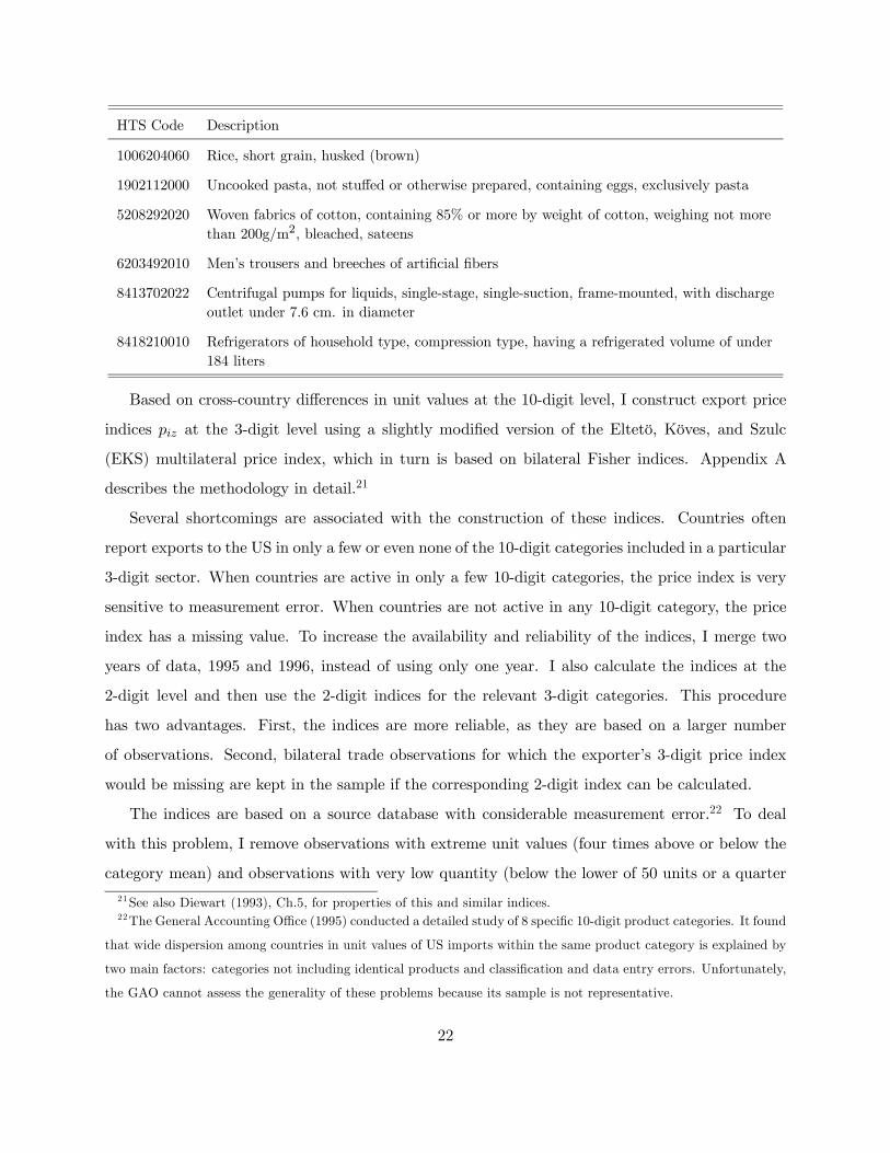
HTS Code Description

1006204060 Rice, short grain, husked (brown)

1902112000 Uncooked pasta, not stuffed or otherwise prepared, containing eggs, exclusively pasta

5208292020 Woven fabrics of cotton, containing 85% or more by weight of cotton, weighing not morethan 200g/m2, bleached, sateens

6203492010 Men’s trousers and breeches of artificial fibers

8413702022 Centrifugal pumps for liquids, single-stage, single-suction, frame-mounted, with dischargeoutlet under 7.6 cm. in diameter

8418210010 Refrigerators of household type, compression type, having a refrigerated volume of under184 liters

Based on cross-country differences in unit values at the 10-digit level, I construct export price

indices piz at the 3-digit level using a slightly modified version of the Eltetö, Köves, and Szulc

(EKS) multilateral price index, which in turn is based on bilateral Fisher indices. Appendix A

describes the methodology in detail.21

Several shortcomings are associated with the construction of these indices. Countries often

report exports to the US in only a few or even none of the 10-digit categories included in a particular

3-digit sector. When countries are active in only a few 10-digit categories, the price index is very

sensitive to measurement error. When countries are not active in any 10-digit category, the price

index has a missing value. To increase the availability and reliability of the indices, I merge two

years of data, 1995 and 1996, instead of using only one year. I also calculate the indices at the

2-digit level and then use the 2-digit indices for the relevant 3-digit categories. This procedure

has two advantages. First, the indices are more reliable, as they are based on a larger number

of observations. Second, bilateral trade observations for which the exporter’s 3-digit price index

would be missing are kept in the sample if the corresponding 2-digit index can be calculated.

The indices are based on a source database with considerable measurement error.22 To deal

with this problem, I remove observations with extreme unit values (four times above or below the

category mean) and observations with very low quantity (below the lower of 50 units or a quarter

21See also Diewart (1993), Ch.5, for properties of this and similar indices.22The General Accounting Office (1995) conducted a detailed study of 8 specific 10-digit product categories. It found

that wide dispersion among countries in unit values of US imports within the same product category is explained by

two main factors: categories not including identical products and classification and data entry errors. Unfortunately,

the GAO cannot assess the generality of these problems because its sample is not representative.

22

of the category mean quantity). Lastly, aggregation problems may still be present at the 10-digit

level, but I expect these problems to be minimized at the 10-digit level of aggregation.

Table A1 provides summary measures of the export price indices. Ordering countries by income,

and normalizing the indices so that Canada has a value of 1 in every sector, the table shows the

geometric average of the sectoral indices for each goods category. Graphs 2a to 2c provide the

same information. The correlation between export price indices and income is positive for all

Differentiated sectors, and for most of Reference-priced and Homogenous sectors. The average

correlation across sectors is 0.45 for Differentiated sectors, 0.36 for Reference-priced sectors, and 0.23

for Homogeneous sectors. This is consistent with the supply-side assumptions of most theoretical

trade models accounting for vertical differentiation, and it confirms the findings of Hummels and

Klenow (2002) and Schott (2004). The average across sectors of the cross-country dispersion of

price indices is also higher for Differentiated sectors (0.43) than for Reference-priced (0.40) and

Homogeneous (0.34) sectors.23 For any given country, there is also considerable variation in export

prices across sectors. The average across countries of the cross-sector dispersion of price indices is

0.49 for Differentiated goods, 0.40 for Referenced-priced goods, and 0.35 for Homogeneous goods.24

4.2 Empirical Specification

Quality differences are presumably one of the main sources of cross-country variation in export

prices. However, this variation might also reflect differences in prices for goods of the same quality,

which might stem, for example, from differences in production costs. I postulate a reduced-form

specification for the determination of the export price that includes both quality level and exporter

income per capita. The inclusion of the latter variable attempts to capture cross-country variation

in production costs systematically related to income. Distance of country i to the US is also included

to control for selection bias in the quality composition of exports to the US. Export prices are thus

determined by:

ln piz = ζ0z + ζ1z ln θiz + ζ2z ln yi + ζ3z lnDistUSi + ξiz. (17)

The partial relationship between product quality and export price is given by ζ1z. Since it is23Dispersion measures are calculated taking the logarithm of the indices. Thus, their magnitude does not depend

on which particular country is used to normalize.24The MATLAB code used to construct the indices and the detailed tables with the export price indices sector by

sector are available online: http://www.econ.lsa.umich.edu/~hallak/papers.html

23

more costly to produce goods of higher than of lower quality, we expect this relationship to be

positive. The sign of ζ2z is instead ambiguous. Once we control for product quality, differences in

comparative advantage are likely to drive any systematic relationship between income and produc-

tion costs (and hence export prices). The relationship can take either sign. Higher income countries

often have a comparative advantage in capital-intensive sectors, as they tend to be capital abun-

dant. In those sectors, higher income implies stronger comparative advantage, and a lower export

price. We thus expect ζ2z < 0. For other (labor-intensive) sectors, higher income is associated with

comparative disadvantage. We thus expect ζ2z > 0. The caveat about the inappropriateness of a

sectoral understanding of comparative advantage also applies here. But it now applies more force-

fully since it affects the empirical specification. Once we introduce quality differences, sectors might

not be either capital or labor intensive. Within a sector, high quality varieties might be capital

intensive while low quality varieties are labor intensive. More generally, we expect the relationship

between income and production costs to vary according to quality. The constant parameter ζ2z in

(17) can only capture the sectoral average of this (quality-dependent) relationship.

The distance to the US is included in (17) to capture the Alchian-Allen conjecture. In the

presence of quality differences, trade costs might not be proportional to price. In particular, if

transport costs depend on weight, these costs will be lower as a fraction of price for high quality

goods. The quality composition of exports will then depend on the magnitude of transport costs,

which in turn depends on the distance between trading partners. Hummels and Skiba (2003)

provide evidence on the empirical relevance of this conjecture. In our sample of unit values of US

imports, this might induce selection bias as only high quality varieties will be exported to the US

by distant countries. Hence, controlling for a country’s average quality of exports to all countries

(θiz), a larger distance to the US will imply a higher quality selection of exports to that market,

and thus a higher observed price index piz. We thus expect a positive sign for ζ3z.25

The main advantage of using export price indices, compared to the use of income in the previous

section, is that their cross-sector variation is able to capture variation across sectors in quality

supply. However, there is considerable measurement error in the price indices, and their reliability

as price measures is yet untested. The indices will be a very noisy indicator of quality if the variance

25The assumption of uniform quality within country-sector in fact rules out the Alchian-Allen effect. I still include

distance to the US to prevent this effect from causing selection bias in the estimation.

24

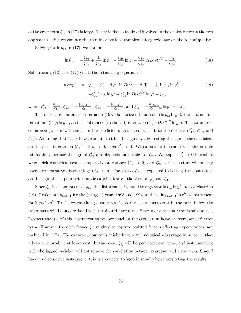
of the error term ξiz in (17) is large. There is then a trade-off involved in the choice between the two

approaches. But we can use the results of both as complementary evidence on the role of quality.

Solving for ln θiz in (17), we obtain:

ln θiz = −ζ0zζ1z

+1

ζ1zln piz −

ζ2zζ1z

ln yi −ζ3zζ1z

lnDistUSi − ξizζ1z

. (18)

Substituting (18) into (12) yields the estimating equation:

ln impkiz = ϕiz + ψkz − eσzηz lnDistki + βzI

ki + ζ 01z ln piz ln y

k (19)

+ζ 02z ln yi ln yk + ζ 03z lnDistUSi ln yk + ξ0iz,

where ζ 01z =eσzµzζ1z

, ζ 02z = −eσzµzζ2zζ1z

, ζ 03z = −eσzµzζ3zζ1z

, and ξ0iz = −eσzµzζ1z

ξiz ln yk + eσzνki .

There are three interaction terms in (19): the “price interaction” (ln piz ln yk), the “income in-

teraction” (ln yi ln yk), and the “distance (to the US) interaction” (lnDistUSi ln yk). The parameter

of interest µz is now included in the coefficients associated with these three terms (ζ01z, ζ

02z, and

ζ 03z). Assuming that ζ1z > 0, we can still test for the sign of µz by testing the sign of the coefficient

on the price interaction (ζ 01z). If µz > 0, then ζ 01z > 0. We cannot do the same with the income

interaction, because the sign of ζ 02z also depends on the sign of ζ2z. We expect ζ02z > 0 in sectors

where rich countries have a comparative advantage (ζ2z < 0) and ζ 02z < 0 in sectors where they

have a comparative disadvantage (ζ2z > 0). The sign of ζ03z is expected to be negative, but a test

on the sign of this parameter implies a joint test on the signs of µz and ζ3z.

Since ξiz is a component of piz, the disturbance ξ0iz and the regressor ln piz ln y

k are correlated in

(19). I calculate piz,t−1 for the (merged) years 1993 and 1994, and use ln piz,t−1 ln yk as instrument

for ln piz ln yk. To the extent that ξiz captures classical measurement error in the price index, the

instrument will be uncorrelated with the disturbance term. Since measurement error is substantial,

I expect the use of this instrument to remove much of the correlation between regressor and error

term. However, the disturbance ξiz might also capture omitted factors affecting export prices, not

included in (17). For example, country i might have a technological advantage in sector z that

allows it to produce at lower cost. In that case, ξiz will be persistent over time, and instrumenting

with the lagged variable will not remove the correlation between regressor and error term. Since I

have no alternative instrument, this is a concern to keep in mind when interpreting the results.

25

4.3 Estimation results

I estimate (19) using 2SLS, sector by sector and pooling across sectors. I first focus on Differentiated

goods, and impose the restrictions that ζ2z = 0 and ζ3z = 0, thus keeping only the price interaction.

Under these restrictions, it is only differences in quality (plus a random disturbance) that drive

differences in export prices.26 This is primarily a benchmarking exercise to compare the performance

of the price interaction with the performance of the income interaction (as used in the previous

section). The first row of Table 7 shows the results. Comparing them with those of Table 1, we

find that the number of positive and negative estimated coefficients is very similar. However, the

estimates using exporter price are on average less precisely estimated; while in Table 1 there are

only 35 sectors with non-significant coefficients, there are 54 of these sectors when price is used

instead of income. The last two columns of Table 7 show the results of the pooled regression, where

only the coefficient on the price interaction is constrained to be the same across sectors. The first

of these columns shows the unweighted 2SLS results. The second column shows estimation results

with observations weighted according to the precision of the price index. Denoting by Giz the

number of active 10-digit categories used in the construction of piz, I assume that the precision of

piz is positively related to Giz, and use weights w =pln(Giz). In both cases, results are reported

with heteroskedasticity-robust standard errors and clustering by country pair. The unweighted and

weighted regressions show similar results. Both coefficient estimates are positive and statistically

significant at the 5% level. Maintaining the assumption that ζ1 > 0, this implies that µ > 0.

The lower precision of the sector-by-sector estimates of Table 7 compared to those of Table 1

suggests that, since export prices are correlated with income, the price interaction might be merely

picking up the explanatory power of the (omitted) income interaction, itself unrelated to quality.

The second specification deals with this concern by including both the price and income interactions

(still imposing ζ3z = 0). The results are shown below in Table 7. When both price and income

interactions are included, the price interaction retains considerable explanatory power. In the

sectoral regressions, the sign of the price interaction is still positive in the same number of sectors,

even though the number of them with significantly positive coefficient decreases substantially. The

change is even stronger, however, for the estimates of the income interaction. The coefficient is less

often positive, and it is positive and significant in only a few more sectors than it is negative and

26A previous version of this paper (Hallak 2003) implicitly imposed these restrictions.

26

significant. Furthermore, the coefficient on the income interaction is more affected by the inclusion

of the price interaction than viceversa. This is consistent with the prediction. Once export prices

are controlled for, the sign of the income interaction depends on the relationship between income

and production costs, and is no longer expected to be uniformly positive.

In the pooled regression, only the coefficient on the price interaction is constrained to be the

same across sectors. The coefficients on all other variables are free to take sector-specific values. In

particular, the coefficient on the income interaction is allowed to vary across sectors to control for

the (sector-specific) average relationship between income and production costs. In the unweighted

estimation, we cannot reject the null that µ = 0. This in part reflects the fact that, while the

coefficient on the price interaction is positive in almost 2/3 of the sectors, it is still negative in a

substantial number of them (39). But it might also reflect the fact that, in sectors where the price

indices are not accurately measured, the income interaction might end up misleadingly capturing,

because of its correlation with the price interaction, the quality effect that the price term is unable

to capture itself. This is partly supported by the results of the last column, where both the

magnitude and the significance of the coefficient increase as observations are weighted according to

the precision of the price measure.

The last set of results corresponds to the full specification, where distance to the US is measured

by the distance from capital cities to New York. The results here are slightly more consistent with

the theoretical predictions. The coefficient on the price interaction is more often positive and

significant and less often negative and significant, while the median across sectors increases. The

estimates for the income interaction are unaffected, except for a decrease in the median magnitude.

The coefficient on the distance interaction is weekly consistent with the Alchian-Allen prediction;

it is more often negative than positive, and more often negative and significant than positive and

significant. The median coefficient is also negative. In most of the sectors, however, the estimates

are statistically insignificant. Since the empirical specification captures the Alchian-Allen effect

only indirectly–as it is not designed for that purpose–it is not surprising that it fails to identify

this effect with precision.

The pooled estimates resemble those of the previous specification. The unweighted regression

yields a positive but statistically insignificant coefficient (the p-value is 0.11). But the coefficient

on the price interaction is significant at the 5% level when observations are weighted according

27

to the precision of the export price index. The difference between the unweighted and weighted

results for the price interaction suggests that measurement error in the export price indices might

be an important reason explaining the paucity of significantly positive coefficients in the sectoral

regressions. In addition, the substantial change in the estimates for the income interaction term

when the price interaction is included in the regression further support the idea that quality drives

the (stronger) results of section 3. It is nevertheless appropriate here to keep in mind two strong

caveats already raised. First, the estimates may be biased due to the correlation between the

disturbance term and the instrument (the lagged price interaction). Second, the coefficient on

the interaction term fails to capture the quality-dependent nature of the relationship between

production costs and income.

Table 8 shows the results of estimating (19) using OLS and alternative measures of GDP and

distance to the US. The OLS estimates are in the top panel. The sector-by-sector regressions

show that the coefficient on the price interaction is less often positive and less often significant,

while the coefficient on the income interaction is more often positive and more often positive and

significant. The median coefficient also decreases for the price interaction and increases for the

income interaction. In contrast to the sectoral results, the pooled regressions show an increase in

both the magnitude and significance of the estimated coefficients for the price interaction term.

The middle panel shows results using per capita GDP not adjusted for purchasing power parity.

The results are not very sensitive to which measure is used. The most salient change is that the

coefficient on the price interaction in the weighted pooled regression is now significant at only the

10% level (the higher variance of this alternative GDP measure explains the smaller magnitude of

the estimates). Finally, the bottom panel shows results when distance to the closest US coast (Los

Angeles or New York) is used as an alternative measure of distance to the US. Here, the results are

almost unchanged.

Even though the baseline results in Table 7 are in general consistent with the theoretical pre-

diction, the sign of the estimated coefficient has the opposite sign in many sectors. In 14 of these

sectors, the estimates are significantly different from zero. To evaluate whether sectors with similar

results have common characteristics, Graph 3 groups the 114 sectors into 11 broader categories.

For each of these groups, the upper bar summarizes the results for the coefficient on the price

interaction and the lower bar for the coefficient on the income interaction. The part of the bar to

28

the right (left) of the vertical center line counts the number of sectors with positive (negative) coef-

ficients. Darker colors represent significant coefficients. The results are systematic for some of these

groups. For example, the sign of the coefficient on the price interaction is positive, as predicted,

in all 17 sectors in the group “Textiles, Apparel, and Footwear”. It is positive and significant in

14 of these sectors. In “Chemicals”, the coefficient is positive in 6 out of 7 sectors, and positive

and significant in 3. In contrast, the coefficient tends to be negative in the groups “Household

Appliances and Electronics” (5 out of 6), “Electrical Machinery and Apparatus” (6 out of 7), and

“Professional and Scientific Equipment” (5 out of 7). There is no single convincing explanation for

the observed pattern of results. Since prices are measured with considerable error, if in the latter

sectors most of the cross-country variation of export prices is due to quality differences and not to

differences in production costs, then the information conveyed by cross-country variation in export

prices not already contained in the variation of income may consist of mere noise. In that case,

the income interaction might end up capturing most of the quality effect. Although in principle

appealing, this explanation presumes–without evidence supporting it–that export prices reflect

mostly quality instead of costs in these sectors. In addition, it fails to explain why the estimated

coefficient is significantly negative in some sectors. The coefficient on the income interaction tends

to be negative, as predicted, in groups such as “Food and Beverages” and “Textiles, Apparel, and

Footwear”, where it is plausible that lower income countries have a comparative advantage. It tends

to be positive in groups such “Agricultural and Industrial Machinery” and “Electrical Machinery

and Apparatus”, where we expect higher income countries to have a comparative advantage.

Table 9 shows the results of estimating (19) for Reference-priced and Homogeneous sectors

(the top panel replicates results for Differentiated sectors shown in Table 7). For Referenced-price

sectors, the distribution of the estimated coefficient on the price interaction in terms of sign and

significance is similar to the case of Differentiated sectors. The coefficient is positive in 2/3 of

the sectors (35) and positive and significant in 1/3 (14). However, the median magnitude of the

estimated coefficient almost doubles the median for Differentiated goods. This result is confirmed

by the pooled regression estimates; the coefficient is positive and significant at the 1% level in both

the unweighted and weighted regressions. The coefficient on the income interaction term is now

more often negative than positive and the median magnitude is negative. This is consistent with the

theoretical prediction if higher income is a source of comparative disadvantage in a higher proportion

29

of Reference-priced sectors than of Differentiated sectors. Finally, the distance interaction gives

stronger support to the Alchian-Allen conjecture. In sum, the results for Reference-priced sectors

are consistent with the main theoretical prediction. But the theory would also predict weaker rather

than stronger results than those for Differentiated sectors.

As in the previous section, the estimates are very different for Homogeneous goods. Both the

coefficient on the price interaction and on the income interaction are in more sectors negative than

positive. They are almost never significant. The distance term is negative in most sectors, but it

is also not significant. In all three cases, the median coefficient is negative.

5 Conclusions and Further Comments

A substantial amount of theoretical work predicts that product quality plays an important role

as a determinant of the direction of trade. This paper provides evidence supporting the empirical

relevance of this prediction. A key aspect of the paper is its strategy for identifying unobserved

cross-country differences in product quality. Exporter income per capita is first used as a proxy,

yielding results that are consistent with the theoretical prediction in a majority of Differentiated-

good sectors: rich countries tend to import relatively more from countries that produce high quality

goods. These results can be interpreted as a sector-level confirmation of the Linder hypothesis.

Furthermore, the inability of typical specifications using aggregate data to control for inter-sectoral

determinants of comparative advantage explains the failure so far to find empirical support for this

hypothesis.

Concerns about forces other than quality driving the results are addressed in two ways. First,

still using income as proxy for quality, the estimation is performed on Referenced-priced sectors,

where the theory can reasonably be expected to apply, and on Homogeneous sectors, where the

theory should not apply. The results are strongly consistent with the predictions. Second, export

price indices are used as indicators of quality. The results here are weaker, but they are still

consistent with the predictions. An overall assessment of the evidence presented in the paper

provides a compelling case for quality as a significant factor explaining global patterns of bilateral

trade.

Further research will hopefully improve many aspects of the theoretical framework and empir-

30

ical strategy used here. First, an advantage of the proposed demand system is its simplicity for

capturing income effects on quality choice. However, it could be extended to allow for more flexible

substitution patterns, in particular, closer substitutability between goods of similar quality. This

possibility is ruled out here, which might explain why, in several sectors, the results contradict

the theoretical prediction. Second, as suggested by the theoretical work on trade with vertical

differentiation, it is not merely the mean but the entire distribution of income that matters as a

determinant of international trade. Third, the accuracy and reliability of the export price indices

used in this study is yet untested. Since unit values are likely to be the best, although indirect,

available source of information on cross-country differences in quality levels covering a broad range

of goods, further research focused on these indices seems necessary and promising.

References

[1] Bergstrand, J. (1989), “The Generalized Gravity Equation, Monopolistic Competition, and

the Factor-Proportions Theory of International Trade,” Review of Economics and Statistics,

71 (1), 143-153.

[2] Brooks, E. (2003), “Why Don’t Firms Export More? Product Quality and Colombian Plants,”

UC Santa Cruz, mimeo.

[3] Cogan, J. (1981), “Fixed Costs and Labor Supply,” Econometrica, 49, 945-963.

[4] Dalgin, M., Mitra, D., and V. Trindade (2004), “Inequality, Nonhomothetic Preferences, and

Trade: A Gravity Approach,” mimeo.

[5] Deardorff, A. (1984), “Testing Trade Theories and Predicting Trade Flows,” in R.W.Jones and

P.B.Kenen, ed., Handbook of International Economics, Vol.1, (Amsterdam, Elsevier).

[6] Deardorff, A. (1998), “Determinants of Bilateral Trade: Does Gravity Work in a Neoclassical

World?,” in J. Frankel, ed., The Regionalization of the World Economy, (Chicago, Chicago

University Press).

[7] Diewert, W. (1993), “Index Numbers,” in W. Diewert and A. Nakamura, Essays in Index

Number Theory, Vol. 1, (Amsterdam, Elsevier Science Publishers B.V.).

31

[8] Falvey, R. and H. Kierzkowski (1987), “Product Quality, Intra-industry Trade and (Im)perfect

Competition,” in H. Kierzkowski, ed., Protection and Competition in International Trade,

(Oxford: Basil Blackwell).

[9] Feenstra, R, Romalis, J., and P. Schott (2002), “US Imports, Exports, and Tariff Data, 1989-

2001,” NBER Working Paper 9387.

[10] Feenstra, R. (2000), “World Trade Flows, 1980-1997,” Center for International Data, Institute

of Governmental Affairs, UC Davis.

[11] Flam, H., and E. Helpman (1987), “Vertical Product Differentiation and North-South Trade,”

American Economic Review, 77 (5), 810-822.

[12] Francois, J. and S. Kaplan (1996), “Aggregate Demand Shifts, Income Distribution, and the

Linder Hypothesis,” Review of Economics and Statistics, 78, 244-250.

[13] General Accounting Office (1995), “US Imports: Unit Values Vary Widely for Identically

Classified Commodities,” Report GAO/GGD-95-90.

[14] Hallak, J. (2003), “The Effect of Cross-Country Differences in Product Quality on the Direction

of International Trade,” RSIE Working Paper 493.

[15] Hummels, D. and P. Klenow (2002), “The Variety and Quality of a Nation’s Exports,” mimeo.

[16] Hummels, D. and A. Skiba (2003), “Shipping the Good Apples Out? An Empirical Confir-

mation of the Alchian-Allen Conjecture,” Purdue University, mimeo. Forthcoming Journal of

Political Economy.

[17] Hunter, L. (1991), “The Contribution of Non-homothetic Preferences to Trade,” Journal of

International Economics, 30, 345-358.

[18] Hunter, L. and J. Markusen (1988), “Per-Capita Income as a Determinant of Trade, in R.

Feenstra, ed., Empirical Methods for International Trade, (Cambridge, MA, MIT Press).

[19] Leamer, E. and J. Levinsohn (1995), “International Trade Theory: The Evidence,” in G.

Grossman and K. Rogoff, ed., Handbook of International Economics, Vol.3, (Amsterdam, El-

sevier).

32

[20] Linder (1961), S., An Essay on Trade and Transformation, (Stockholm: Almqvist & Wiksell).

[21] Markusen, J. (1986), “Explaining the Volume of Trade: An Eclectic Approach,” American

Economic Review, 76 (5), 1002-1011.

[22] Matsuyama, K. (2000), “A Ricardian Model with a Continuum of Goods under Nonhomothetic

Preferences: Demand Complementarities, Income Distribution, and North-South Trade, Jour-

nal of Political Economy, 108 (6), 1093-1120.

[23] McPherson, M., M. Redfearn, and M. Tieslau (2001), “International Trade and Developing

Countries: An Empirical Investigation of the Linder Hypothesis,” Applied Economics, 33,

649-657.

[24] Murphy, K.M. and A. Shleifer (1997), “Quality and Trade,” Journal of Development Eco-

nomics, 53, 1-15.

[25] Rauch, J. (1999), “Networks versus Markets in International Trade,” Journal of International

Economics, 48, 7-35.

[26] Romalis, J. (2004), “Factor Proportions and the Structure of Commodity Trade”, American

Economic Review, 94, 67-97.

[27] Schott, P. (2003), “One Size Fits All? Heckscher-Ohlin Specialization in Global Production,”

American Economic Review, 93, 686-708.

[28] Schott, P. (2004), “Across-Product versus Within-Product Specialization in International

Trade,” Forthcoming Quarterly Journal of Economics.

[29] Shatz, H. (1997), “Note on Distance Data”, Harvard University, mimeo.

[30] Stokey, N. (1991), “The Volume and Composition of Trade between Rich and Poor Countries.”

Review of Economic Studies, 58, 63-80.

33

A Appendix: Methodology of construction of export price indices

A representative 2-digit sector z includes 10-digit categories n = 1, ..., N . Dividing the value by

the quantity of imports in each of these categories, we obtain the unit value (average export price)

pin for country i in category n. Based on 10-digit-level prices pin, I will construct multilateral price

indices piz at the 2-digit level. Country i is “active” in category n if pin is non-missing. Country i

is active in sector z if it has at least two active categories. Otherwise, piz takes a missing value.

There is considerable measurement error in the source database. I use the following procedure

to detect and remove outliers. For each category n, I calculate the geometric mean of unit values

across countries, excluding the observations with maximum and minimum values. I then remove

observations with unit values 4 times above or below the mean. Since observations with extreme

unit values show disproportionately low export quantities, I remove observations with quantity

below the minimum of 50 units or a quarter of the average quantity for the category.

I then take country j as a numeraire. For each other country i, I calculate the bilateral Fisher

price index P ji between i and j, using only their common active categories (P

ji takes a missing value

if i and j do not have any common active category). As a result, I obtain a vector of bilateral price

indices P j , with country j as the numeraire. I repeat this procedure taking alternatively all countries

as numeraire, and obtain vectors P j , j = 1, ..., C, where C is the number of active countries in the

sector. These vectors are separated into three groups. The first group contains vectors j = 1, ..., C1,

those with non-missing values. The second group contains vectors j = C1 + 1, ..., C2, with at most

5 missing values. The third group contains the remaining vectors j = C2 + 1, ...C.

I then follow a three step procedure. I take the first group and normalize each vector to sum

up to 1. Denote normalized vectors by eP j . The geometric weighted average of these vectors is:

P 1z =CYj=1

³ eP j´wj

, (20)

where wj is the number of active categories of country j in sector z. In the second step, I take

each vector P j in the second group and normalize it to sum up to 1 −mj , where mj is the sum

of the entries in P 1z corresponding to the the missing elements in P j . I then impute the values in

P 1z to the missing elements in P j , thus obtaining a normalized (to 1) vector eP j . Using normalized

vectors eP j , j = 1, ...C2, I recalculate (20) and obtain P 2z . In the third step, I repeat the procedure

for the remaining vectors. I finally calculate pz =QC

j=1

³ eP j´wj

, where each element is piz.

34

Table 1: Basic Results OLS - Differentiated goods (114 Sectors)

Regressions by Sector

Pooled Regression

Sign

Significance (5%)

Pos. Neg. Pos. Not Sig. Neg. Median

Coefficient ln(yi)*ln(yk) 78 36 56 35 23 0.1218 0.0782***

(0.0230) ln(Distanceik) 0 114 0 0 114 -1.0451 Borderik 103 11 41 73 0 0.3260 Common Languageik 112 2 95 19 0 0.5366 PTAik 95 19 61 51 2 0.3755 Colonial Linkik 110 4 89 25 0 0.8288 Common Colonyik 88 26 20 92 2 0.3351

Notes: Heteroskedasticity-robust standard errors in all regressions. Clustering by country pair across sectors in pooled regression. Columns 2 and 3 provide a breakdown of the total number of sectors by sign of the estimated coefficient. Columns 4 to 6 provide a breakdown by sign and significance. * Significant at the 10% level ** Significant at the 5% level *** Significant at the 1% level

Table 2: All Sectors OLS - Coefficient on interaction term

Regressions by Sector

Pooled Regression

Sign

Significance (5%)

Pos. Neg. Pos. Not Sig. Neg. Median

Coefficient Differentiated Goods ln(yi)*ln(yk) 78 36 56 35 23 0.1218 0.0782***

(0.0230) Reference Priced Goods ln(yi)*ln(yk) 33 18 17 28 6 0.0776 0.0723***

(0.0252) Homogenous Goods ln(yi)*ln(yk) 18 20 3 29 6 -0.0498 -0.0453

(0.0295)

Notes: Heteroskedasticity-robust standard errors in all regressions. Clustering by country pair across sectors in pooled regression. Columns 2 and 3 provide a breakdown of the total number of sectors by sign of the estimated coefficient. Columns 4 to 6 provide a breakdown by sign and significance. * Significant at the 10% level ** Significant at the 5% level *** Significant at the 1% level

Table 3: Fixed Exporting Costs MLE – Coefficient on interaction term

Regressions by Sector

Sign

Significance (5%)

Pos. Neg. Pos. Not Sig. Neg. Median Differentiated Goods ln(yi)*ln(yk) 72 42 52 36 26 0.0797 Reference Priced Goods ln(yi)*ln(yk) 36 15 24 22 5 0.0661 Homogenous Goods ln(yi)*ln(yk) 12 26 3 24 11 -0.0372

Notes: Heteroskedasticity-robust standard errors in all regressions. Columns 2 and 3 provide a breakdown of the total number of sectors by sign of the estimated coefficient. Columns 4 to 6 provide a breakdown by sign and significance.

Table 4: Sectoral data: Alternative Linder Terms OLS – Coefficient on Linder term (signs reversed)

Regressions by Sector

Pooled Regression

Sign

Significance (5%)

Pos. Neg. Pos. Not Sig. Neg. Median

Coefficient Differentiated Goods ln(yi)*ln(yk) 78 36 56 35 23 0.1218 0.0782***

(0.0230) -|yi-yk| 79 35 55 41 18 0.0118 0.0090***

(0.0025) -ln(|yi-yk|) 77 37 51 44 19 0.0504 0.0343***

(0.0129) -|ln(yi)-ln(yk)| 78 36 58 36 20 0.1530 0.1033***

(0.0273) Reference Priced Goods ln(yi)*ln(yk) 33 18 17 28 6 0.0776 0.0723***

(0.0252) -|yi-yk| 32 19 16 28 7 0.0072 0.0070**

(0.0028) -ln(|yi-yk|) 33 18 14 33 4 0.0327 0.0307**

(0.0143) -|ln(yi)-ln(yk)| 32 19 16 29 6 0.0968 0.0826***

(0.0302) Homogenous Goods ln(yi)*ln(yk) 18 20 3 29 6 -0.0498 -0.0453

(0.0295) -|yi-yk| 15 23 5 26 7 -0.0079 -0.0067**

(0.0034) -ln(|yi-yk|) 18 20 5 29 4 -0.0097 -0.0152

(0.0182) -|ln(yi)-ln(yk)| 17 21 4 27 7 -0.0860 -0.0712**

(0.0357)

Notes: Heteroskedasticity-robust standard errors in all regressions. Clustering by country pair across sectors in pooled regression. Columns 2 and 3 provide a breakdown of the total number of sectors by sign of the estimated coefficient. Columns 4 to 6 provide a breakdown by sign and significance. * Significant at the 10% level ** Significant at the 5% level *** Significant at the 1% level

Table 5: The Aggregation Bias An artificial example

Importer

Machinery

Apparel

Total Exporter

Sweden

(S)

Domin. Rep. (DR)

Total

Exports

Sweden

(S)

Domin. Rep. (DR)

Total Exports

Sweden

(S)

Domin. Rep. (DR)

Total Exports

UK 150 300 450 150 50 200 300 350 650 Lebanon (L) 50 150 200 300 150 450 350 300 650 Total Imports 200 450 650 450 200 650 650 650 1300 Ratio UK/L 3 2 0.5 0.33 0.86 1.17 Ratio of Ratios (UK/L)S /(UK/L)DR

1.5

1.5

0.73

Table 6: Aggregate data - Failure of Standard Test of the Linder Hypothesis OLS - Coefficient on Linder term (signs reversed)

Linder Term

ln(yi)*ln(yk)

-|yi-yk|

-ln|yi-yk|

-|ln(yi)-ln(yk)|

Differentiated Goods -.1812***

(0.0321) -0.0203***

(0.0035) -0.0893***

(0.0197) -0.1953***

(0.0386) Reference Priced Goods -0.0267

(0.0384) -0.0045 (0.0041)

-0.0206 (0.0210)

-0.0254 (0.0453)

Homogenous Goods 0.0726

(0.0489)

0.0062 (0.0054)

0.0110 (0.0271)

0.0690 (0.0560)

Total (All Sectors in Sample)

-0.0447 (0.0298)

-0.0068** (0.0034)

-0.0378** (0.0175)

-0.0574* (0.0349)

Total (All Sectors) -0.0371

(0.0311) -0.0082** (0.0034)

-0.0286 (0.0176)

-0.0406 (0.0358)

Notes: Heteroskedasticity-robust standard errors in all regressions. The coefficients and standard errors in the third column are multiplied by 1,000. * Significant at the 10% level ** Significant at the 5% level *** Significant at the 1% level

Table 7: Price as Indicator of Quality

IV - Differentiated goods

Regressions by Sector Pooled Regression

Sign

Significance (5%)

Pos. Neg. Pos. Not Sig. Neg. Median

Coefficient

(unweighted)

Coefficient (weighted)

Price Only

ln(Pi)*ln(yk) 75 39 44 54 16 0.1880 0.1056** (0.0441)

0.1016** (0.0462)

Price and Income

ln(Pi)*ln(yk) 75 39 33 66 15 0.1858 0.0648 (0.0541)

0.0981* (0.0579)

ln(yi)*ln(yk) 66 48 35 51 28 0.1016

Price, Income, and Distance to US

ln(Pi)*ln(yk) 75 39 36 64 14 0.1923 0.0877 (0.0553)

0.1304** (0.0596)

ln(yi)*ln(yk) 66 48 35 51 28 0.0823

ln(DistiUS)* ln(yk) 53 61 11 87 16 -0.0181

Notes: The lagged export price index (93-94) is used as instrument for the current index (95-96). Heteroskedasticity-robust standard errors in all regressions. Clustering by country pair across sectors in pooled regression. Columns 2 and 3 provide a breakdown of the total number of sectors by sign of the estimated coefficient. Columns 4 to 6 provide a breakdown by sign and significance. * Significant at the 10% level ** Significant at the 5% level *** Significant at the 1% level

Table 8: Robustness IV - Differentiated goods

Regressions by Sector Pooled Regression

Sign

Significance (5%)

Pos. Neg. Pos. Not Sig. Neg. Median

Coefficient (unweighted)

Coefficient (weighted)

OLS

Price, Income, and Distance to US

ln(Pi)*ln(yk) 69 45 34 68 12 0.1582 0.0958** (0.0393)

0.1405*** (0.0455)

ln(yi)*ln(yk) 69 45 47 39 28 0.1113

ln(DistiUS)* ln(yk) 57 57 14 84 16 0.0006

GDP – no PPP adjustment

Price, Income, and Distance to US

ln(Pi)*ln(yk) 73 41 36 64 14 0.1322

0.0472 (0.0351)

0.0720* (0.0382)

ln(yi)*ln(yk) 66 48 34 52 28 0.0228

ln(DistiUS)* ln(yk) 54 60 11 87 16 -0.0125

Distance to closest US coast

Price, Income, and Distance to US

ln(Pi)*ln(yk) 75 39 36 65 13 0.1894

0.0891 (0.0554)

0.1315** (0.0597)

ln(yi)*ln(yk) 66 48 35 52 27 0.0803

ln(DistiUS)* ln(yk) 54 60 13 85 16 -0.0086

Notes: The lagged export price index (93-94) is used as instrument for the current index (95-96). Heteroskedasticity-robust standard errors in all regressions. Clustering by country pair across sectors in pooled regression. Columns 2 and 3 provide a breakdown of the total number of sectors by sign of the estimated coefficient. Columns 4 to 6 provide a breakdown by sign and significance. * Significant at the 10% level ** Significant at the 5% level *** Significant at the 1% level

Table 9: All sectors IV Estimation

Regressions by Sector Pooled Regression

Sign

Significance (5%)

Pos. Neg. Pos. Not Sig. Neg. Median

Coefficient

(unweighted)

Coefficient (weighted)

Differentiated Goods

Price, Income, and Distance to US

ln(Pi)*ln(yk) 75 39 36 64 14 0.1923 0.0877 (0.0553)

0.1304** (0.0596)

ln(yi)*ln(yk) 66 48 35 51 28 0.0823

ln(DistiUS)* ln(yk) 53 61 11 87 16 -0.0181

Reference Priced Goods

Price, Income, and Distance to US

ln(Pi)*ln(yk) 35 16 14 33 4 0.3608

0.3066*** (0.0679)

0.3868*** (0.0771)

ln(yi)*ln(yk) 23 28 9 32 10 -0.0291

ln(DistiUS)* ln(yk) 19 32 5 35 11 -0.0436

Homogeneous Goods

Price, Income, and Distance to US

ln(Pi)*ln(yk) 17 21 0 37 1 -0.1355

-0.0839 (0.1494)

-0.0709 (0.1519)

ln(yi)*ln(yk) 12 26 0 36 2 -0.1369

ln(DistiUS)* ln(yk) 10 28 1 35 2 -0.1186

Notes: The lagged export price index (93-94) is used as instrument for the current index (95-96). Heteroskedasticity-robust standard errors in all regressions. Clustering by country pair across sectors in pooled regression. Columns 2 and 3 provide a breakdown of the total number of sectors by sign of the estimated coefficient. Columns 4 to 6 provide a breakdown by sign and significance. * Significant at the 10% level ** Significant at the 5% level *** Significant at the 1% level

Table A1 Geometric Mean of Sectoral Price Indices

Country GDP per Capita

(PPP) Differentiated Goods Reference Priced Goods Homogenous Goods

Switzerland 25,475 1.64 1.79 1.00 Norway 24,693 1.46 1.47 1.23 Japan 23,211 1.48 1.92 1.31 Canada 23,085 1.00 1.00 1.00 Denmark 22,947 1.51 1.48 1.58 Belgium-Lux. 22,700 1.45 1.41 0.97 Singapore 22,270 1.09 1.26 1.17 Hong Kong 22,166 0.79 1.28 1.06 Austria 22,089 1.43 1.71 1.16 Germany 21,478 1.46 1.49 1.14 Australia 21,267 1.29 1.36 1.00 Netherlands 20,812 1.41 1.39 1.20 Italy 20,512 1.33 1.41 1.25 France 20,492 1.54 1.64 1.42 Sweden 20,030 1.46 1.56 1.49 United Kingdom 19,465 1.39 1.47 1.25 Finland 18,764 1.60 1.39 1.24 New Zealand 17,705 1.30 1.39 0.95 Israel 17,394 1.33 1.57 1.27 Ireland 17,264 1.46 1.76 1.13 Spain 15,163 1.29 1.21 0.93 Portugal 13,613 1.20 1.24 1.12 South Korea 13,502 0.91 1.25 1.28 Taiwan 13,335 0.81 1.38 1.20 Greece 13,147 1.10 1.20 1.13 Saudi Arabia 10,766 1.12 1.27 1.13 Argentina 10,736 1.02 1.10 1.00 South Africa 8,581 1.11 1.19 1.02 Malaysia 8,145 0.94 1.14 1.04 Uruguay 7,831 1.04 0.79 1.02 Chile 7,544 1.00 0.98 1.19 Mexico 7,061 0.74 0.95 1.02 Poland 6,605 0.86 1.11 1.09 Brazil 6,572 0.89 1.07 1.07 Romania 6,430 0.81 0.72 1.02 Thailand 6,217 0.79 1.15 0.96 Colombia 6,151 0.87 1.04 1.11 Venezuela 5,979 0.73 0.89 0.82 Costa Rica 5,940 0.97 1.18 0.92 Turkey 5,803 0.93 1.33 0.98 Bulgaria 5,608 0.91 0.86 0.79 Tunisia 4,870 1.02 1.36 1.36 Paraguay 4,598 0.83 0.48 0.83 Peru 4,329 1.02 1.06 0.98 Dominican Rep. 3,997 0.87 0.93 0.89 Lebanon 3,964 0.94 1.13 1.13 Philippines 3,518 0.89 1.06 0.92 Guatemala 3,444 0.87 0.98 0.90 Syria 3,211 1.06 1.40 0.93 Ecuador 3,162 0.89 1.02 0.89 Morocco 3,052 0.94 1.34 2.37* Indonesia 2,869 0.80 1.01 0.88 Egypt 2,869 1.05 0.88 0.68 Sri Lanka 2,741 0.70 1.06 1.11 China 2,560 0.63 1.02 1.06 India 1,877 0.82 0.97 0.87 Pakistan 1,733 0.82 0.70 0.81 Vietnam 1,478 0.70 1.02 0.65 Bangladesh 1,253 0.76 1.34 0.58 Nigeria 832 0.81 0.97 0.73

Average correlation b/w sectoral index and GDP Per Capita

0.45

0.36

0.23

Note: The bottom row gives the average across sectors of the correlation between PPP GDP per capita and the price index. * Morocco has price indices for only two sectors.

Table A2. List of 3-digit SITC sectors included Differentiated sample (some 4-digit sectors may be excluded)

Sector Description Sector Description

34 Fish,fresh (live or dead),chilled or frozen 727 Food processing machines and parts 48 Cereal prepar. & preps. Of flour of fruits or veg. 728 Mach.& Equipment specialized for particular ind. 56 Vegetab.,roots & tubers,prepared/preserved,n.e.s. 736 Mach.tools for working metal or met.carb., Parts 73 Chocolate & other food preptns. Containing cocoa 741 Heating & cooling equipment and parts 98 Edible products and preparations n.e.s. 742 Pumps for liquids.liq.elevators and parts

111 Non alcoholic beverages,n.e.s. 743 Pumps & compressors,fans & blowers,centrifuges 248 Wood,simply worked,and railway sleepers of wood 744 Mechanical handling equip.and parts 431 Animal & vegetable oils and fats,processed & waxes 745 Other non-electrical mach.tools,apparatus & parts 533 Pigments,paints,varnishes & related materials 749 Non-electric parts and accessories of machines 541 Medicinal and pharmaceutical products 751 Office machines 551 Essential oils,perfume and flavour materials 752 Automatic data processing machines & units thereof 553 Perfumery,cosmetics and toilet preparations 759 Parts of and accessories suitable for 751--or 752- 554 Soap,cleansing and polishing preparations 761 Television receivers 591 Disinfectants,insecticides,fungicidesweed killers 762 Radio-broadcast receivers 598 Miscellaneous chemical products,n.e.s. 764 Telecommunications equipment and parts 611 Leather 771 Electric power machinery and parts thereof 612 Manufactures of leather/of composition leather nes 772 Elect.app.such as switches,relays,fuses,pwgs etc. 621 Materials of rubber(e.g.,pastes.plates,sheets,etc) 773 Equipment for distributing electricity 625 Rubber tyres,tyre cases,etc.for wheels 774 Electric apparatus for medical purposes,(radiolog) 628 Articles of rubber,n.e.s. 775 Household type,elect.& Non-electrical equipment 635 Wood manufactures,n.e.s. 776 Thermionic,cold & photo-cathode valves,tubes,parts 642 Paper and paperboard,cut to size or shape 778 Electrical machinery and apparatus,n.e.s. 651 Textile yarn 781 Passenger motor cars,for transport of pass.& Good 652 Cotton fabrics,woven 782 Motor vehicles for transport of goods/materials 653 Fabrics,woven,of man-made fibres 783 Road motor vehicles,n.e.s. 654 Textil.fabrics,woven,oth.than cotton/man-made fibr 784 Parts & accessories of 722-,781--,782-,783- 655 Knitted or crocheted fabrics 785 Motorcycles,motor scooters,invalid carriages 656 Tulle,lace,embroidery,ribbons,& other small wares 786 Trailers & other vehicles,not motorized 657 Special textile fabrics and related products 791 Railway vehicles & associated equipment 658 Made-up articles,wholly/chiefly of text.materials 792 Aircraft & associated equipment and parts 659 Floor coverings,etc. 793 Ships,boats and floating structures 661 Lime,cement,and fabricated construction materials 812 Sanitary,plumbing,heating,lighting fixtures 662 Clay construct.materials & refractory constr.mate 821 Furniture and parts thereof 663 Mineral manufactures,n.e.s 831 Travel goods,handbags,brief-cases,purses,sheaths 665 Glassware 842 Outer garments,mens,of textile fabrics 666 Pottery 843 Outer garments,womens,of textile fabrics 667 Pearls,precious& semi-prec.stones,unwork./worked 844 Under garments of textile fabrics 673 Iron and steel bars,rods,angles.shapes & sections 845 Outer garments and other articles,knitted 678 Tubes,pipes and fittings,of iron or steel 846 Under garments,knitted or crocheted 679 Iron & steel castings,forgings & stampings;rough 847 Clothing accessories of textile fabrics 691 Structures& parts of struc.;iron,steel,aluminium 848 Art.of apparel & clothing accessories,no textile 692 Metal containers for storage and transport 851 Footwear 694 Nails,screws,nuts,bolts etc.of iron.steel,copper 871 Optical instruments and apparatus 695 Tools for use in hand or in machines 872 Medical instruments and appliances 696 Cutlery 874 Measuring,checking,analysing instruments 697 Household equipment of base metal,n.e.s. 881 Photographic apparatus and equipment,n.e.s. 699 Manufactures of base metal,n.e.s. 882 Photographic & cinematographic supplies 711 Steam & other vapour generating boilers & parts 884 Optical goods,n.e.s. 713 Internal combustion piston engines& parts 885 Watches and clocks 714 Engines & motors,non-electric 892 Printed matter 716 Rotating electric plant and parts 893 Articles of materials described in division 58 721 Agricultural machinery and parts 894 Baby carriages,toys,games and sporting goods 722 Tractors fitted or not with power take-offs, etc. 895 Office and stationery supplies,n.e.s. 723 Civil engineering & contractors plant and parts 896 Art,collectors pieces & antiques 724 Textile & leather machinery and parts 897 Jewellery,goldsmiths and other art. Of precious m. 725 Paper & pulp mill mach.,mach for manuf.of paper 898 Musical instruments,parts and accessories 726 Printing & bookbinding mach.and parts 899 Other miscellaneous manufactured articles

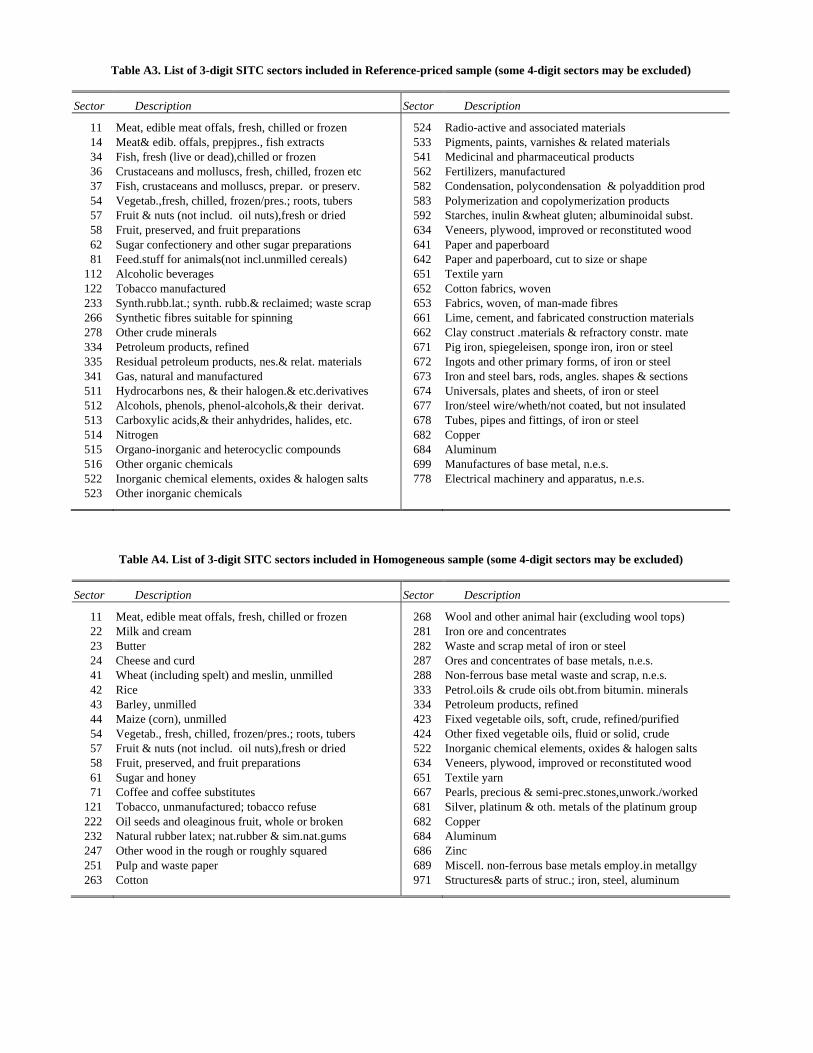
Table A3. List of 3-digit SITC sectors included in Reference-priced sample (some 4-digit sectors may be excluded)

Sector Description Sector Description

11 Meat, edible meat offals, fresh, chilled or frozen 524 Radio-active and associated materials 14 Meat& edib. offals, prepjpres., fish extracts 533 Pigments, paints, varnishes & related materials 34 Fish, fresh (live or dead),chilled or frozen 541 Medicinal and pharmaceutical products 36 Crustaceans and molluscs, fresh, chilled, frozen etc 562 Fertilizers, manufactured 37 Fish, crustaceans and molluscs, prepar. or preserv. 582 Condensation, polycondensation & polyaddition prod 54 Vegetab.,fresh, chilled, frozen/pres.; roots, tubers 583 Polymerization and copolymerization products 57 Fruit & nuts (not includ. oil nuts),fresh or dried 592 Starches, inulin &wheat gluten; albuminoidal subst. 58 Fruit, preserved, and fruit preparations 634 Veneers, plywood, improved or reconstituted wood 62 Sugar confectionery and other sugar preparations 641 Paper and paperboard 81 Feed.stuff for animals(not incl.unmilled cereals) 642 Paper and paperboard, cut to size or shape

112 Alcoholic beverages 651 Textile yarn 122 Tobacco manufactured 652 Cotton fabrics, woven 233 Synth.rubb.lat.; synth. rubb.& reclaimed; waste scrap 653 Fabrics, woven, of man-made fibres 266 Synthetic fibres suitable for spinning 661 Lime, cement, and fabricated construction materials 278 Other crude minerals 662 Clay construct .materials & refractory constr. mate 334 Petroleum products, refined 671 Pig iron, spiegeleisen, sponge iron, iron or steel 335 Residual petroleum products, nes.& relat. materials 672 Ingots and other primary forms, of iron or steel 341 Gas, natural and manufactured 673 Iron and steel bars, rods, angles. shapes & sections 511 Hydrocarbons nes, & their halogen.& etc.derivatives 674 Universals, plates and sheets, of iron or steel 512 Alcohols, phenols, phenol-alcohols,& their derivat. 677 Iron/steel wire/wheth/not coated, but not insulated 513 Carboxylic acids,& their anhydrides, halides, etc. 678 Tubes, pipes and fittings, of iron or steel 514 Nitrogen 682 Copper 515 Organo-inorganic and heterocyclic compounds 684 Aluminum 516 Other organic chemicals 699 Manufactures of base metal, n.e.s. 522 Inorganic chemical elements, oxides & halogen salts 778 Electrical machinery and apparatus, n.e.s. 523 Other inorganic chemicals

Table A4. List of 3-digit SITC sectors included in Homogeneous sample (some 4-digit sectors may be excluded)

Sector Description Sector Description

11 Meat, edible meat offals, fresh, chilled or frozen 268 Wool and other animal hair (excluding wool tops) 22 Milk and cream 281 Iron ore and concentrates 23 Butter 282 Waste and scrap metal of iron or steel 24 Cheese and curd 287 Ores and concentrates of base metals, n.e.s. 41 Wheat (including spelt) and meslin, unmilled 288 Non-ferrous base metal waste and scrap, n.e.s. 42 Rice 333 Petrol.oils & crude oils obt.from bitumin. minerals 43 Barley, unmilled 334 Petroleum products, refined 44 Maize (corn), unmilled 423 Fixed vegetable oils, soft, crude, refined/purified 54 Vegetab., fresh, chilled, frozen/pres.; roots, tubers 424 Other fixed vegetable oils, fluid or solid, crude 57 Fruit & nuts (not includ. oil nuts),fresh or dried 522 Inorganic chemical elements, oxides & halogen salts 58 Fruit, preserved, and fruit preparations 634 Veneers, plywood, improved or reconstituted wood 61 Sugar and honey 651 Textile yarn 71 Coffee and coffee substitutes 667 Pearls, precious & semi-prec.stones,unwork./worked

121 Tobacco, unmanufactured; tobacco refuse 681 Silver, platinum & oth. metals of the platinum group 222 Oil seeds and oleaginous fruit, whole or broken 682 Copper 232 Natural rubber latex; nat.rubber & sim.nat.gums 684 Aluminum 247 Other wood in the rough or roughly squared 686 Zinc 251 Pulp and waste paper 689 Miscell. non-ferrous base metals employ.in metallgy 263 Cotton 971 Structures& parts of struc.; iron, steel, aluminum

Graph 1:

Histogram of OLS Estimates of Interaction Term Coefficient

0

5

10

15

20

25

<0.5 -0.5 - -0.4

-0.4 - -0.3

-0.3 --0.2

-0.2 --0.1

-0.1 - 0

0 - 0.1

0.1 -0.2

0.2 -0.3

0.3 - 0.4

0.4 - 0.5

>0.5

Differentiated Goods Reference Priced Goods Homogenous Goods

Graphs 2a-2c: Relationship Between Average Price Indices and Income per Capita

Differentiated Goods

-0.75

-0.5

-0.25

0

0.25

0.5

0.75

6.5 7 7.5 8 8.5 9 9.5 10 10.5

ln(Income per Capita)

ln(A

vera

ge P

rice

Inde

x)

Reference Priced Goods

-0.75

-0.5

-0.25

0

0.25

0.5

0.75

6.5 7 7.5 8 8.5 9 9.5 10 10.5

ln(Income per Capita)

ln(A

vera

ge P

rice

Inde

x)

Homogenous Goods

-0.75

-0.5

-0.25

0

0.25

0.5

0.75

6.5 7 7.5 8 8.5 9 9.5 10 10.5

ln(Income per Capita)

ln(A

vera

ge P

rice

Inde

x)

Graph 3: Distribution of Coefficients by Group

Note: The upper and lower bars in each group show the distribution of the coefficients on the price and income interactions by size and significance levels, respectively.

20 15 10 5 0 5 10 15 20

5020 15 10 5 10 15 20

Food and Beverages

Chemicals

Textiles, Apparel and Footwear

Agricultural and Industrial Machinery

Household Appliances and Electronics

Electrical Machinery and Apparatus

Road Vehicles and Transportation Equipment

Professional and Scientific Equipment

Miscellaneous Manufactures

Manuf. of Leather, Rubber, Cork, Wood and Paper

Manuf. of Metals and Non-metallic Minerals

Significantly negative

Not significant

Significantly positive

Number of sectors