Product Line Design for Consumer Durables: An …lluo/ProductLine_Final.pdf · 1 Product Line...
38
1 Product Line Design for Consumer Durables: An Integrated Marketing and Engineering Approach Lan Luo March 2010 Forthcoming in Journal of Marketing Research _________________________________________________________________ Lan Luo is an Assistant Professor of Marketing, at the Marshall School of Business, University of Southern California, Los Angeles, CA 90089. The author greatly appreciates P.K. Kannan, Babak Besharati, Shapour Azarm for their valuable inputs to this research. She also wishes to thank the editors-in-chief, the associate editors, the four anonymous reviewers, and seminar attendants at the 2006 INFORMS Marketing Science conference, the 2006 INFORMS Annual Meeting, the 2007 Product and Service Innovations Conference in Utah, the 2008 Research Frontiers in Marketing Science Conference at University of Texas at Dallas, the 2008 Marketing Innovations Conference at Rensselaer Polytechnic Institute for their constructive comments and helpful guidance.
Transcript of Product Line Design for Consumer Durables: An …lluo/ProductLine_Final.pdf · 1 Product Line...
1
Product Line Design for Consumer Durables: An Integrated Marketing and Engineering Approach
Lan Luo
March 2010
Forthcoming in Journal of Marketing Research
_________________________________________________________________
Lan Luo is an Assistant Professor of Marketing, at the Marshall School of Business, University of Southern California, Los Angeles, CA 90089.
The author greatly appreciates P.K. Kannan, Babak Besharati, Shapour Azarm for their valuable inputs to this research. She also wishes to thank the editors-in-chief, the associate editors, the four anonymous reviewers, and seminar attendants at the 2006 INFORMS Marketing Science conference, the 2006 INFORMS Annual Meeting, the 2007 Product and Service Innovations Conference in Utah, the 2008 Research Frontiers in Marketing Science Conference at University of Texas at Dallas, the 2008 Marketing Innovations Conference at Rensselaer Polytechnic Institute for their constructive comments and helpful guidance.

1
Abstract Product line design for consumer durables often relies on close coordination between marketing and engineering domains. Product lines that evolve as “optimal” from marketers’ perspective may not be “optimal” from an engineering viewpoint, and vice versa. Although extant research has proposed sophisticated techniques to handle problems that characterize each individual domain, the majority of these developments have not addressed the interdependent issues across marketing and engineering. We present a product line optimization method that enables managers to simultaneously consider factors deemed as important from both domains of marketing and engineering. One major advantage of this method is that it takes into account the strategic reactions from the incumbent manufacturers and the retailer in the design of the product line. We demonstrate in a simulation study that this method is applicable to problems with a reasonably large scale. Using data collected in a power tool development project undertaken by a major U.S. manufacturer, we illustrate that the proposed method leads to a more profitable product line than alternative approaches that consider requirements from these two domains separately. Keywords: Product Line, New Products, Product Design, Marketing Engineering Integration,
Optimization Methods, Genetic Algorithm, Simulated Annealing
2
Product line design is a critical decision that determines many firms’ successes (Hauser,
Tellis and Griffin 2006). In a product line design project, close coordination between the
marketing and engineering domains is essential. For example, when designing a power tool
product line, the product designer must take into account not only consumers’ preferences for the
product’s features and prices, but also other important engineering issues such as whether the
products are safe and robust in a variety of usage environments. Similar argument can be applied
to many consumer durable products such as toys, appliances, trucks, airplanes, laptops, and etc.
In the design of a product line, such marketing and engineering considerations are often
highly interdependent. For example, a consumer may think about a power tool in terms of
attributes such as power amp and product life, whereas an engineering designer may think of
these same concepts in terms of technical variables such as housing, gear ratio and gearbox type.
Such highly interconnected relationships between the two domains imply that any required
action in one domain can potentially influence the outcomes in the other domain. Therefore, in
the design of an optimal or near-optimal product line, the marketing and engineering
requirements often cannot be pursued separately or even sequentially.
Despite the compelling need for a unified framework that integrates design
considerations from both disciplines concurrently, the vast majority of extant research has
emphasized issues from the perspective of each individual discipline. This discipline-centric
focus is largely determined by the complexity of the overall product line design problem. When
designing a line of consumer durable products, firms need to account for not only the
interrelationships between consumer preferences and engineering feasibility/restrictions in the
design of each individual product, but also the revenue and cost interactions across the products
in the product line. Furthermore, in order to accurately forecast the revenue from a product line,
3
it is critical to account for the strategic reactions from competing manufacturers and the retailer
when the new product line enters into the market. Within this context, a simultaneous
consideration of all these essential issues across both disciplines is considerably challenging both
conceptually and computationally.
The primary goal of this research is to propose a product line optimization method to
tackle this combinatorial challenge. In particular, we propose a procedure in which the marketing
and engineering criteria are considered concurrently in the search for a profit-maximizing
product line. We demonstrate in a simulation study that this method is applicable to problems
with a reasonably large scale. Using data collected in a power tool development project
undertaken by a major U.S. manufacturer, we illustrate that the proposed method leads to a more
profitable product line than alternative approaches that consider requirements from these two
domains separately.
The rest of the paper is organized as follows. First, we discuss the relationship of this
paper to extant literature and the contribution of this research. Second, we present the details of
our product line optimization. Third, we describe a simulation study in which we investigate the
computational characteristics of our method. Next, we describe the empirical application. We
conclude by summarizing contributions and discussing limitations and future research.
RELATIONSHIP TO EXISTING RESEARCH
There are four streams of research related to this paper. The first stream investigates
product line design from a marketing perspective (e.g. Balakrishnan, Gupta, and Jacob 2004,
2006; Belloni, Freund, Selove, and Simester 2008; Chen and Hausman 2000; Dobson and Kalish
1988 and 1993; Green and Krieger 1985; Kannan, Pope, and Jain 2009; McBride and Zufryden
1988; Moore, Louviere, and Verma 1999; Nair, Thakur and Wen 1995; Steiner and Hruschka

4
2003). This research stream utilizes conjoint data and searches for an optimal or near-optimal
product line by selecting levels of consumer attributes. The second stream of papers examines
the product line design problem with an engineering focus (e.g. Farrell and Simpson 2003; Rai
and Allada 2003; Simpson, Seeperad, and Mistree 2001). This line of research has generally
focused on platform management in which researchers strive for balance between the
commonality of the product platform and the individual product’s engineering performance. The
third stream consists of papers investigating how to integrate engineering and marketing
considerations into the design of a single product (e.g. Besharati, Luo, Azarm, and Kannan 2004
and 2006; Griffin and Hauser 1993; Hauser and Clausing 1988; Li and Azarm 2000; Luo,
Kannan, Besharati, and Azarm 2005; Michalek, Feinberg, and Papalambros 2005; Srinivasan,
Lovejoy, and Beach 1997; Tarasewich and McMullen 2001; Tarasewich and Nair 2001). Finally,
the fourth stream consists of papers that aim to incorporate marketing and engineering
considerations in a product line design (e.g. D’Souza and Simpson 2003; Farrell and Simpson
2009; Heese and Swaminathan 2006; Jiao and Zhang 2005; Kumar, Chen, and Simpson 2009; Li
and Azarm 2002; Michalek, Feinberg, Ebbes, Adiguzel, and Papalambros 2009; Michalek,
Ceryan, Papalambros, and Koren 2006).
In the following we discuss how our paper extends the four streams of research.
From a substantive perspective, we contribute to the literature by providing an effective
coordination of a number of essential issues across both disciplines of marketing and
engineering. Specifically, on the marketing side, we evaluate the market potential of the product
line by 1) modeling consumers’ heterogeneous product preferences; and 2) estimating how the
competing manufacturers and the retailer will respond to the launch of the new product line. On

5
the engineering side, we focus on 1) ensuring the engineering feasibility and robustness of the
products; and 2) maximizing the cost synergy across the products in the product line.
Given the complex nature of product line design, our optimization method by no means
exclusively accounts for all the marketing and engineering criteria currently being considered in
the design of a product line. We focus on the above issues due to their considerable significance
in the product design literature. Since any of these issues can have a substantial impact on the
profitability of the final product line, we contribute to the literature by tackling the combinatorial
challenge of integrating these essential issues across both disciplines of marketing and
engineering. Particularly, one major advantage of the proposed model is that it directly accounts
for the strategic responses from the competing manufacturers and the retailer. Although
recognized as an important challenge in product line design problem (Belloni et al. 2008), these
issues have never been addressed in previous work.
From a methodological perspective, we contribute to the literature by searching for an
optimal product line in a large design space with a mix of discrete and continuous design
variables. Due to the complexity of the product line design problem, a number of previous
researchers have limited the composition of a product line within a fairly small set of initial
products (e.g. Kumar et al. 2009; Morgan, Daniels, and Kouvelis 2001; Ramdas and Sawhney
2001). In practice, however, the product design space for a consumer durable product can be
very large or virtually infinite. In attempts to address this issue, Michalek et al. (2006 and 2009)
proposed an analytical target cascading (ATC) method that enables the search of an optimal
product line in a complex design space. Although the ATC method is highly efficient in
coordinating marketing and engineering considerations (we will demonstrate this in a simulation
study), it is not directly applicable in a product design space with discrete product attributes.

6
Therefore, one major advantage of our method is its ability to accommodate both discrete and
continuous variables in a large design space. However, the approach we take comes with the cost
of combinatorial complexity. The ability of this method to scale up to a large problem is
discussed later in the paper.
PROPOSED METHOD
Following Kaul and Rao (1995) and Michalek et al. (2009), we begin by defining a set of
consumer attributes and design variables as the starting point of our model. The vector of
consumer attributes (denoted as x) represents all the attributes directly considered by consumers
in a product purchase decision (e.g. power amp, product life). The identification of these
attributes follows the typical procedure used to determine which product attributes will be
included in a conjoint experiment. And the design variables (denoted as y) are variables that the
product designer needs to decide upon in the design of a product (e.g. gear ratio, housing type).
These variables determine the values of the consumer attribute vector (excluding brand and price)
and are collectively needed for proper functioning of the product. Next, we proceed to define an
engineering response function r(y) that calculates the values of x as a function of y (i.e. x=r(y)).
As discussed by Michalek et al. (2009), while the specification of the response function r(y)
needs to be determined on a case-by-case basis, the general principles of such mapping are well
established in the literature (see Web Appendix A for additional implementation details). Given
the set of design variables (y), consumer attributes (x), and their interrelationships (x=r(y)), the
focal problem of our product line optimization is to determine the design variable configuration
and the wholesale price of each product in the product line under a set of marketing and
engineering criteria.
7
In the following we first describe the specifics of our marketing and engineering
considerations. We then demonstrate how we merge these considerations into a product line
optimization procedure.
Marketing Considerations
From the marketing side, we take into account: 1) how consumers form their preferences
towards each product; and 2) how the competitors and the retailer respond to the launch of the
new product line.
Consumer Preference Model
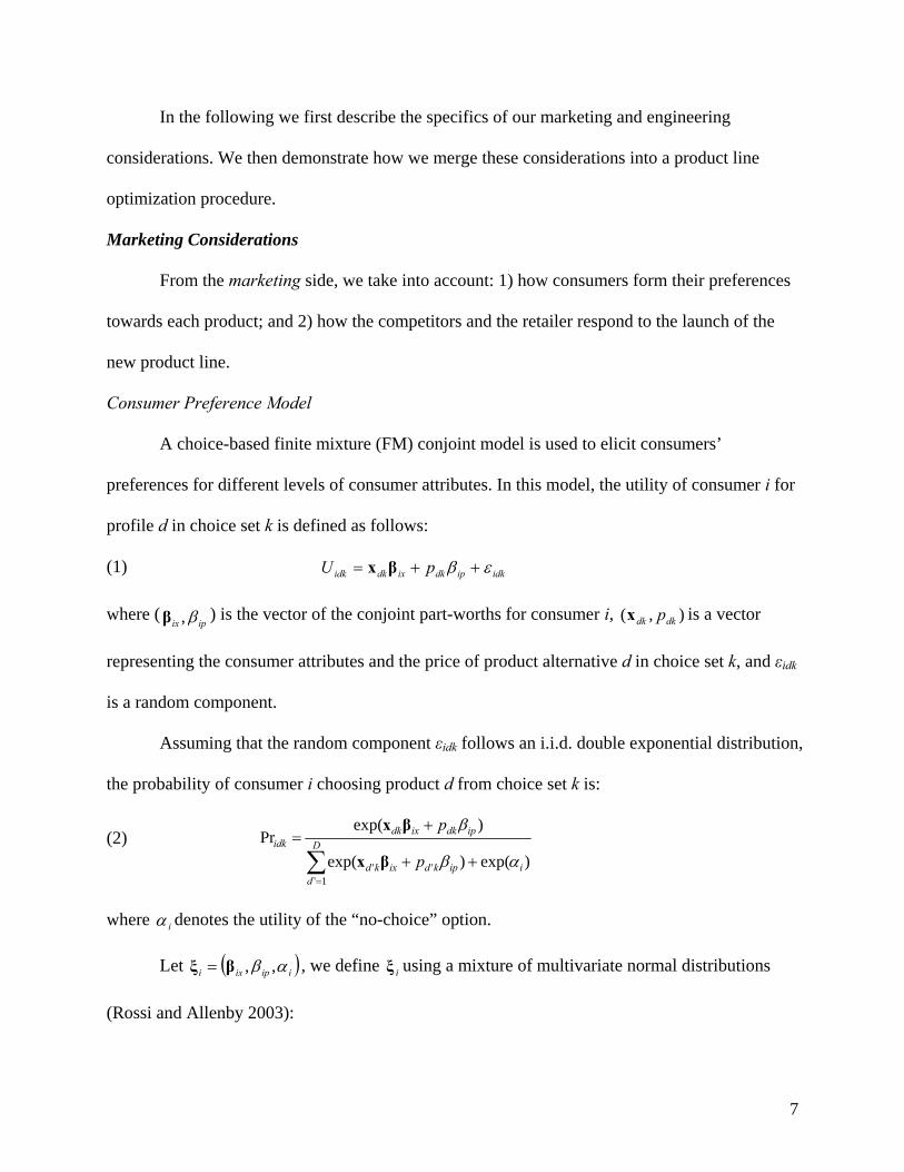
A choice-based finite mixture (FM) conjoint model is used to elicit consumers’
preferences for different levels of consumer attributes. In this model, the utility of consumer i for
profile d in choice set k is defined as follows:
(1) idkipdkixdkidk pU βx
where (ipix ,β ) is the vector of the conjoint part-worths for consumer i, ),( dkdk px is a vector
representing the consumer attributes and the price of product alternative d in choice set k, and εidk
is a random component.
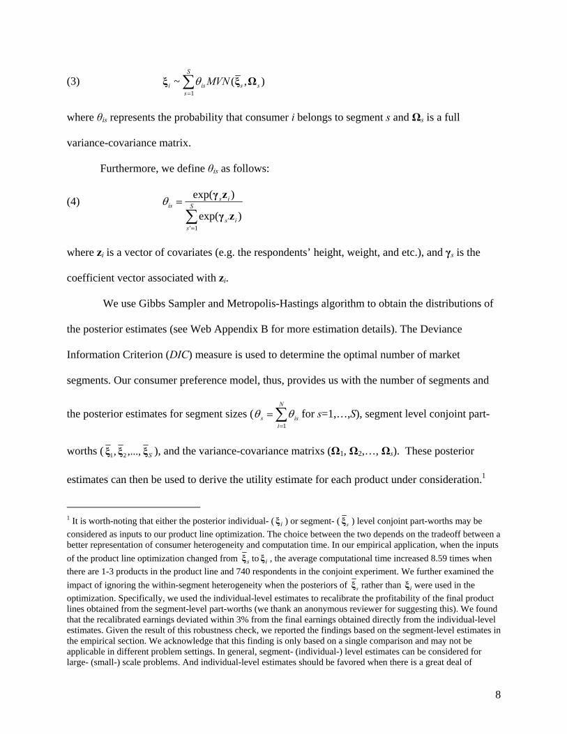
Assuming that the random component εidk follows an i.i.d. double exponential distribution,
the probability of consumer i choosing product d from choice set k is:
(2)
D
diipkdixkd
ipdkixdkidk
p
p
1''' )exp()exp(
)exp(Pr
βx
βx
where i denotes the utility of the “no-choice” option.
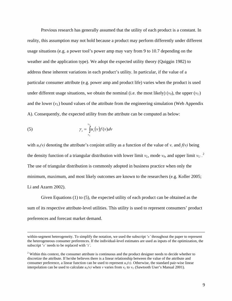
Let iipixi ,,βξ , we define iξ using a mixture of multivariate normal distributions
(Rossi and Allenby 2003):
8
(3) ),(~1
ss
S
sisi MVN Ωξξ
where θis represents the probability that consumer i belongs to segment s and Ωs is a full
variance-covariance matrix.
Furthermore, we define θis as follows:
(4)
S
sis
isis
1'' )exp(
)exp(
zγ
zγ
where zi is a vector of covariates (e.g. the respondents’ height, weight, and etc.), and γs is the
coefficient vector associated with zi.
We use Gibbs Sampler and Metropolis-Hastings algorithm to obtain the distributions of
the posterior estimates (see Web Appendix B for more estimation details). The Deviance
Information Criterion (DIC) measure is used to determine the optimal number of market
segments. Our consumer preference model, thus, provides us with the number of segments and
the posterior estimates for segment sizes (
N
iiss
1
for s=1,…,S), segment level conjoint part-
worths ( Sξξξ ,...,, 21 ), and the variance-covariance matrixs (Ω1, Ω2,…, Ωs). These posterior
estimates can then be used to derive the utility estimate for each product under consideration.1
1 It is worth-noting that either the posterior individual- ( iξ ) or segment- ( sξ ) level conjoint part-worths may be
considered as inputs to our product line optimization. The choice between the two depends on the tradeoff between a better representation of consumer heterogeneity and computation time. In our empirical application, when the inputs
of the product line optimization changed from sξ to iξ , the average computational time increased 8.59 times when
there are 1-3 products in the product line and 740 respondents in the conjoint experiment. We further examined the
impact of ignoring the within-segment heterogeneity when the posteriors of sξ rather than iξ were used in the
optimization. Specifically, we used the individual-level estimates to recalibrate the profitability of the final product lines obtained from the segment-level part-worths (we thank an anonymous reviewer for suggesting this). We found that the recalibrated earnings deviated within 3% from the final earnings obtained directly from the individual-level estimates. Given the result of this robustness check, we reported the findings based on the segment-level estimates in the empirical section. We acknowledge that this finding is only based on a single comparison and may not be applicable in different problem settings. In general, segment- (individual-) level estimates can be considered for large- (small-) scale problems. And individual-level estimates should be favored when there is a great deal of
9
Previous research has generally assumed that the utility of each product is a constant. In
reality, this assumption may not hold because a product may perform differently under different
usage situations (e.g. a power tool’s power amp may vary from 9 to 10.7 depending on the
weather and the application type). We adopt the expected utility theory (Quiggin 1982) to
address these inherent variations in each product’s utility. In particular, if the value of a
particular consumer attribute (e.g. power amp and product life) varies when the product is used
under different usage situations, we obtain the nominal (i.e. the most likely) (v0), the upper (vU)
and the lower (vL) bound values of the attribute from the engineering simulation (Web Appendix
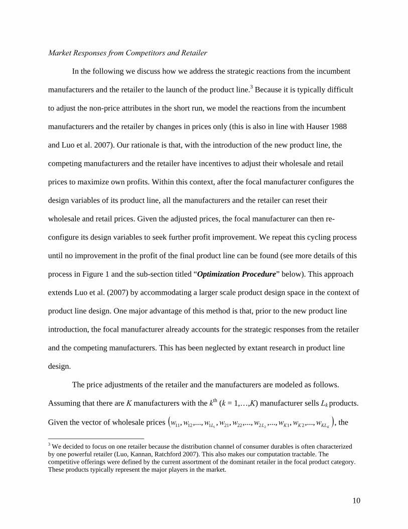
A). Consequently, the expected utility from the attribute can be computed as below:
(5) dvvfvuU
L
v
v
ss )(
with us(v) denoting the attribute’s conjoint utility as a function of the value of v, and f(v) being
the density function of a triangular distribution with lower limit vL, mode v0, and upper limit vU .2
The use of triangular distribution is commonly adopted in business practice when only the
minimum, maximum, and most likely outcomes are known to the researchers (e.g. Koller 2005;
Li and Azarm 2002).
Given Equations (1) to (5), the expected utility of each product can be obtained as the
sum of its respective attribute-level utilities. This utility is used to represent consumers’ product
preferences and forecast market demand.
within-segment heterogeneity. To simplify the notation, we used the subscript ‘s’ throughout the paper to represent the heterogeneous consumer preferences. If the individual-level estimates are used as inputs of the optimization, the subscript ‘s’ needs to be replaced with ‘i’. 2 Within this context, the consumer attribute is continuous and the product designer needs to decide whether to discretize the attribute. If he/she believes there is a linear relationship between the value of the attribute and consumer preference, a linear function can be used to represent us(v). Otherwise, the standard pair-wise linear interpolation can be used to calculate us(v) when v varies from vL to vU (Sawtooth User’s Manual 2001).
10
Market Responses from Competitors and Retailer
In the following we discuss how we address the strategic reactions from the incumbent
manufacturers and the retailer to the launch of the product line.3 Because it is typically difficult
to adjust the non-price attributes in the short run, we model the reactions from the incumbent
manufacturers and the retailer by changes in prices only (this is also in line with Hauser 1988
and Luo et al. 2007). Our rationale is that, with the introduction of the new product line, the
competing manufacturers and the retailer have incentives to adjust their wholesale and retail
prices to maximize own profits. Within this context, after the focal manufacturer configures the
design variables of its product line, all the manufacturers and the retailer can reset their
wholesale and retail prices. Given the adjusted prices, the focal manufacturer can then re-
configure its design variables to seek further profit improvement. We repeat this cycling process
until no improvement in the profit of the final product line can be found (see more details of this
process in Figure 1 and the sub-section titled “Optimization Procedure” below). This approach
extends Luo et al. (2007) by accommodating a larger scale product design space in the context of
product line design. One major advantage of this method is that, prior to the new product line
introduction, the focal manufacturer already accounts for the strategic responses from the retailer
and the competing manufacturers. This has been neglected by extant research in product line
design.
The price adjustments of the retailer and the manufacturers are modeled as follows.
Assuming that there are K manufacturers with the kth (k = 1,…,K) manufacturer sells Lk products.
Given the vector of wholesale prices KKLKKLL wwwwwwwww ,...,,,...,,...,,,,...,, 212222111211 21
, the
3 We decided to focus on one retailer because the distribution channel of consumer durables is often characterized by one powerful retailer (Luo, Kannan, Ratchford 2007). This also makes our computation tractable. The competitive offerings were defined by the current assortment of the dominant retailer in the focal product category. These products typically represent the major players in the market.

11
retailer chooses the retail price of each product in its assortment to maximize own profit. The
retailer’s profit maximization can be written as:
(6)
K
kk
T
t
K
k
L
l
ttklklkl
r
ppppLscrDwpm
k
KKLKL 11 1 1,...,,...,,...,
1/)(*max11111
(7) with
S
ss
K
k
L
lsplksxlk
spklsxklskl
k
p
pm
1
1' 1'''
'''
'
)exp()exp(
)exp('
βx
βx
where πr is the category profit of the retailer, mkl represents the market share of the lth product
from the kth manufacturer, pkl and wkl denote this product’s retail and wholesale prices, Dt is the
overall market demand in year t, r is a discount rate, and sc is the marginal shelf cost. Following
Gordon (2009), we assume that Dt is observed and determined exogenously (as a function of the
products’ replacement cycles, overall economic condition, and etc.). The parameters
sspsxs ,,,β in Equation (7) correspond to posterior conjoint part-worth estimates obtained
from the finite mixture Bayesian estimation.
Given the vector of new retail prices KKLKL pppp ,...,,...,,..., 1111 1
, each manufacturer (k =
1,…,K) will adjust the wholesale prices of the Lk products in its product line to maximize its
profit. Note that this differs from Luo et al. (2007) in that the manufacturer will choose a set of
wholesale prices rather than a single price.
(8) k
T
t
L
l
ttklklkl
mk
wwwFrDmcw
k
kkLkk
1 1,...,,
1/**)(max21
k = 1,…, K
where ckl is the variable cost of the lth product from manufacturer k, Fk is the fixed cost of this
manufacturer.
Similar to Luo et al. (2007), the new wholesale and retail prices are estimated by solving
Equations (6) and (8) iteratively (details in Web Appendix B). A major challenge faced by all
12
existing research in product line design is that multi-product firms with logit demand do not have
log-supermodular profit functions (Hanson and Martin 1996). Therefore, we face the possibility
of multiple price equilibria in our solutions. To alleviate this issue, researchers can empirically
investigate the shapes of the profit functions and run the algorithm with different initial prices in
attempts to move from a local optimum to a better solution. It is also worth-noting that, since we
only account for the retailer and the incumbents’ potential reactions in price adjustments, this
method does not apply in situations where the incumbents change their non-price attributes in
response to the entry of the new product line.
Engineering Considerations
From the engineering side, we take into account: 1) the feasibility and robustness of each
product in the product line; and 2) the cost synergy across the products in the product line.
Engineering Feasibility and Robustness
It is well-established in the engineering literature (e.g. Kouvelis and Yu 1997; Ulrich and
Eppinger 2004) that one essential goal of product design in many product categories (e.g. power
tools, cars, appliances) is to ensure that products will remain feasible and robust under a variety
of usage situations (e.g. different weather conditions and application types). Therefore, our
primary engineering consideration is to evaluate whether each product under consideration
satisfies the feasibility and robustness criteria imposed by the engineering designer. A common
approach to assess whether a product will satisfy these criteria is to examine the lower and upper
bounds of its engineering performance metrics (e.g. motor temperature, motor output speed),
which are created as an output of the design simulation (see Web Appendix A).
In particular, the goal of our feasibility criteria is to ensure that all the products in the
product do not break down under any known usage situation. Let 111211 ,...,, Lyyy
denote the

13
design variable configurations of the L1 products in the focal manufacturer’s product line (i.e. we
set k=1 for the focal manufacturer). Adopted from Besharati, et al. (2004) and (2006), the
feasibility criteria associated with each product can be expressed as follows (h is the index for
the hth feasibility criterion):
(9) 0)],(,0max[1
1
H
hlhg pay
with UPLW papapa ; l = 1,…, L1
where y1l denotes the the design variable vector, pa represents the vector of the engineering
parameters ranging from the lower bound paLW and the upper bound paUP, and g is a dummy
variable indicating whether the product violates the feasibility criterion (g = 1 if violated; g = 0
otherwise).
Following Besharati et al. (2004, 2006) and Ulrich and Eppinger (2004), the vector of
engineering parameters “pa” characterize the uncontrollable variations in the product’s usage
environment. A product line will be penalized in the optimization if it contains any product
violating any of the H constraints.
Our robustness criteria ensure that undesirable variations in the product’s engineering
performance are limited to a reasonably small amount. A product satisfies the robustness criteria
if the undesirable variations of its engineering performance metrics are bounded within the limits
specified by the product designer. Following Besharati et al. (2004) and (2006), the mathematical
representation of the robustness criteria is given in Equation (10):
(10) Jblblb fff
),(),(max 011 paypay
with b =1,…,B; UPLW papapa ; l = 1,…, L1

14
where the index b (b =1,…,B) denotes the bth robustness constraint,
),(),(max 011 paypay lblb ff is the observed maximum variation in the product’s engineering
performance when the engineering parameters deviate from the nominal value 0pa , and Jbf
denotes the maximum acceptable variation specified by the engineering designer. A product line
will be penalized in the optimization if it contains any product violating any of the B constraints.
Cost Synergy
Given the increasing popularity of platform production (Morgan et al. 2001), our cost
model is constructed for platform-based product categories. Within this context, the
manufacturer purchases the components from outside vendors, assembles the components into
the final products, provides after-sale maintenance support, and salvages the product at the end
of its life cycle. Accordingly, the variable cost of product l is computed as follows:
(11) slmlal
R
rrwlrwll ccccvc
11 *)1( l = 1,…, L1
In Equation (11), the variable cost lvc1 is jointly determined by the component cost rwlc
( r is the index for the component, e.g. motor type; and w is the index for the type of the
component, e.g. motor #1), a discount factor rwl associated with component sharing, the
assembly cost alc , the maintenance cost mlc , and the salvage cost slc .
In the platform-management literature, researchers generally refer to the parts firms use
to build the product as components. For example, the major components related to a power tool
are things like motor, gearbox, housing, and etc. Because they define the product from the
designer’s perspective, within our context, these components are essentially a part of the
product’s design variables. When different products within a product line share the same types of
15
components, the cost associated with acquiring each unit of the shared component is scaled down
due to economy of scale. We use a discount factor rwl to capture this effect. In Web Appendix B,
we provide more details on how to define rwl and the other cost elements in Equation (11).
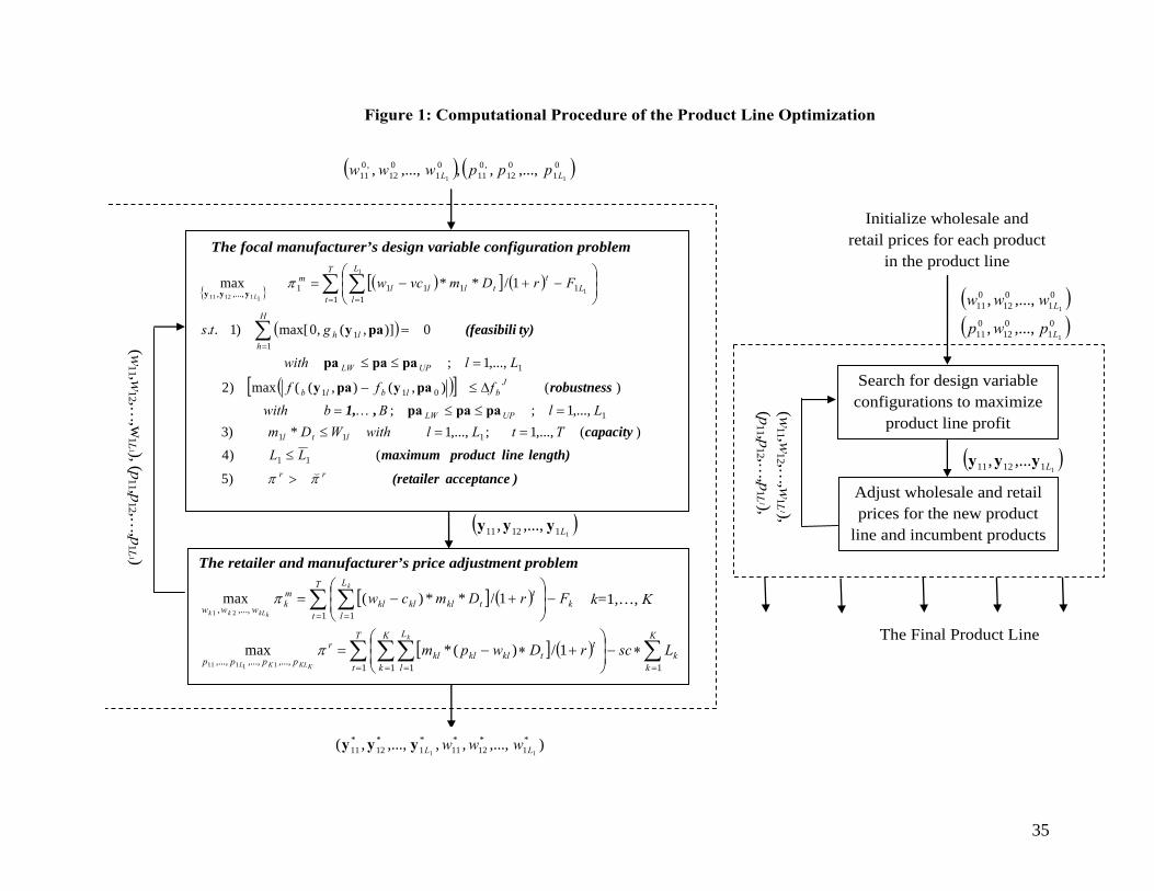
Optimization Procedure
The overall procedure of our product line optimization is provided in Figure 1. As shown
in this figure, the proposed product line optimization includes two inner loop optimizations
(denoted as the focal manufacturer’s design variable configuration problem and the retailer and
manufacturers’ price adjustment problem) and an outer loop optimization (i.e. the iterative
procedure that solves the two inner optimizations iteratively until convergence).
This optimization starts with initializing the vectors of wholesale prices 01
012
011 1
,...,, Lwww
and retail prices 01
012
011 1
,...,, Lppp for the focal manufacturer (denoted as the first manufacturer,
i.e. k = 1). Given these initial wholesale prices, the focal manufacturer searches for vectors of
design variables 111211 ,...,, Lyyy to maximize its product line profit, subject to a set of
constraints (i.e. first block of Figure 1). The first two constraints ensure that each product in the
product line satisfies the engineering feasibility and robustness criteria. The third constraint is the
capacity constraint. Note that the assembly of platform products typically requires different
machine setup for each product. Therefore, we set the capacity constraint based on the
production of each product (i.e. W1l) rather than the sum of production across all the products in
the product line. When a product’s market demand exceeds the capacity constraint, the product’s
production volume will be set at the level of the capacity constraint. The fourth constraint sets
the maximum length of the product line (i.e. 1L ), which is typically pre-specified by the focal
manufacturer. A number of previous papers assumed a fixed number of products in the product
line (e.g. Balakrishnan et al. 2004; Belloni et al. 2008). We relax this assumption by allowing an
16
upper limit of product line length. Finally, the channel acceptance criterion is determined by
comparing the retailer’s new category profit with its current category profit (denoted as r ).
The outputs of this inner loop optimization are the vectors of the design variables
111211 ,...,, Lyyy and their corresponding non-price consumer attributes
111211 ,...,, Lxxx . Next, the
retailer and the manufacturers (including the focal and the competing manufacturers) adjust the
retail and wholesale prices in response to the market entry of this product line (second block of
Figure 1).
Given the adjusted prices, the focal manufacturer re-searches vectors of design variables
to maximize its product line profit. This cycling process continues until no improvement in the
profit of the final product line results. This outer loop optimization is depicted by the dotted box
in Figure 1.
<Insert Figure 1 about here>
This procedure is performed for each possible product line length. The final product line
is chosen as the one that maximizes the firm’s profit as the product line length varies from 1 to
1L . Note that if product line length is fixed (as in Balakrishnan et al. 2004 and Belloni et al.
2008), we only need to perform the optimization once. Additionally, although the retailer may
only consider part of the product line as acceptable, we indirectly accounted for this because the
shorter product line lengths have been considered under this procedure.
Due to the NP-hard property of the product line design (Kohli and Sukumar 1990), the
primary goal of previous research in this area has been finding near-optimal solutions in a
reasonable amount of time. We follow this line of work by using heuristic methods to solve the
focal manufacturer’s design variable configuration problem (first block of Figure 1) and gradient
search methods to search for the adjusted wholesale and retail prices (second block of Figure 1).
17
Although past research has suggested that the heuristic methods of genetic algorithm and
simulated annealing do have the ability to escape from a locally optimal solution (Belloni et al.
2008; Balakrishnan et al. 2004), the solutions provided by these methods do not ensure global
optimality. Similarly, multiple price equilibria may exist when the manufacturers and the retailer
make price adjustments. Therefore, we cannot guarantee a global maximum in our optimization
results. This is a common limitation shared by all extant research in product line design. To
alleviate this issue, researchers can run the optimization multiple times with different starting
values to assess the overall quality of the final solution. On a related note, because the focal
manufacturer’s ultimate goal is to maximize its profit and multiple product lines may generate
identical (or highly similar) profits, the quality of the final solution is evaluated by the earning
levels associated with the product line (Belloni et al. 2008) rather than the closeness in the
configurations of the products. In a similar spirit, the convergence criterion of our product
optimization is based on the level of the final earning rather than the closeness of the solutions.
SIMULATION STUDY
In this section we examine the computational characteristics of the proposed optimization
procedure using simulated data. The primary goals of this simulation study are to empirically
investigate: 1) the use of different computational algorithms in the focal manufacturer’s design
variable configuration problem (the first block of Figure 1); 2) the applicability of the overall
procedure to large scale problems; and 3) the convergence property of this procedure. All the
computations were conducted in Matlab on a Pentium 4 personal computer.
First, we compared the performance of three algorithms in the focal manufacturer’s
design variable configuration problem (the first block of Figure 1). Note that because this
comparison is only related to the first block of Figure 1, the wholesale prices and the retail

18
markups were assumed to be fixed so that we can confine our comparison to this particular part
of the overall problem. Specifically, genetic algorithm (GA), simulated annealing (SA), and
analytical target cascading (ATC) were included in our comparison because previous research
has shown that these methods perform well in product line design problems (e.g. Balakrishnan et
al. 2004; Belloni et al. 2008; and Michalek et al. 2009). In this simulation study, the focal
manufacturer designs a product line consisting of 1 to 8 products, each composed of 4 design
variables (we will extend this to include more design variables in the second part of the
simulation study). Because the ATC method only handles continuous design variables, we
investigated 16 different problem sizes (8 with a mix of discrete and continuous variables and 8
with continuous variables only). For each problem size, we created 5 problem instances, which
results in a total of 80 simulated problems. Web Appendix C provides more details of our
simulation procedure and a brief description of these optimization methods.
Table 1 provides the result comparisons. When the design variable vector included both
discrete and continuous attributes, the average earnings of the product lines were quite
comparable, regardless whether GA or SA was used to solve the optimization. However, in terms
of CPU time, GA is much more efficient than SA. These findings are consistent across different
problem sizes. When the design variable vector included only continuous attributes, the same
pattern resulted between the methods of GA and SA. Note that the results of our comparison for
these two algorithms are also in line with the findings of Belloni et al. (2008). It is possible that
the computational inefficiency of SA results from its extensive search process, as SA sometimes
accept product line configurations that reduce earnings in attempts to escape from a local
optimum. With regard to ATC, this method performs quite well in terms of both the quality of
the solutions and the computation time. In particular, we noticed that ATC seems to generate
19
better solutions than GA and SA as the problem size increases. Our conjecture is that, when there
are many products in the product line, the decompositional-based ATC approach facilitates a
more effective and efficient search as compared to the combinatorial-based GA and SA
approaches. Given the findings above, we suggest using GA in the focal manufacturer’s design
variable configuration problem when the products contain both discrete and continuous design
variables. When the products consist of only continuous variables, the ATC method may be
superior, particularly when there are a great number of products in the product line.
<Insert Table 1 about here>
We further investigated the computation time required to obtain a final solution based on
our overall procedure (the entire Figure 1) across different problem sizes. In this simulation task,
the focal manufacturer designs a product line consisting of 1 to 8 products, each composed of 4,
8, 12, 16, 20, or 24 design variables. This results in a total of 48 simulation problems. In this task,
we used GA to solve the focal manufacturer’s design variable configuration problem (the first
block of Figure 1). We chose GA because it not only handles both continuous and discrete
design variables but also is computationally desirable. The required computation time for our
overall procedure (the entire Figure 1) varied between 2 to 10.4 hours, as the problem sizes range
from a small problem with 1-3 products and 4-8 design variables to a large problem with 6-8
products and 20-24 design variables (more details in Web Appendix C).
Finally, the proposed procedure converged within a reasonable amount of time for all the
simulation problems discussed above. These results suggest that, by and large, our overall
procedure is applicable to problems with a reasonably large scale.4
4 We also compared the performance of our product line optimization to the global optimum (obtained through complete enumeration) for the case of 4 design variables with 1-2 products in the product line. We limited this comparison to only small scale problems for which the global optimum could be obtained in a reasonable amount of time. The average final earnings from our optimization are at 96% of the true optimum.
20
EMPIRICAL APPLICATION
We applied the proposed product line optimization in a case study using data collected in
a power tool product development project undertaken by a large U.S. manufacturer. Teaming
with our industrial partner, we conducted exploratory research (e.g. field trips, focus group
studies) to identify the set of consumer attributes deemed as the most critical by the end users of
this power tool. The identification of these attributes follows the typical procedure used in
determining which attributes to be included in a conjoint experiment. We discovered that
consumers generally take into account the power tool’s brand, price, power amp, product life,
switch type, and girth type in a purchase decision. More details of the conjoint design are
provided in Web Appendix D.5 Given these consumer attributes, we proceeded to determine the
set of design variables. The following design variables were identified because they determine
the values of the consumer attribute vector and are collectively needed for proper functioning of
the product: motor type, speed reduction unit or gearbox type, gear ratio, switch type, and
housing type. See Web Appendix D for more details on the design space defined by these design
variables.
After identifying the vectors of the consumer attributes and design variables, we
proceeded to establish the mapping between the two vectors. The consumer attributes switch
type and girth type are identical to their corresponding design variables (with a small girth
mapped from a small housing and a large girth mapped from a large housing). As for power amp
and product life, an engineering simulation similar to the one described in Web Appendix A was
used to establish the mapping relations. Specifically, the inputs of the simulation are the
configuration of the design variables motor type, gearbox type, gear ratio. The outputs of the
5 We camouflaged some actual attribute names as well as the values of attribute levels, cost estimates, and capacity constraints to protect the proprietary information of our industrial partner.

21
simulation are the values of the product’s 1) power amp and product life (consumer attributes);
and 2) motor temperature, motor output speed, and mass material removal per application
(engineering performance metrics). The former directly influences consumer’s purchase decision.
The latter were used to evaluate whether the product satisfies the feasibility and robustness
constraints specified by the product designer. The uncontrollable variations in the product’s
usage environment were represented by a set of engineering parameters (see Web Appendix D
for more details). And the outputs of the simulation provided the nominal, the lower, and the
upper bound values of each output variable.
Given the sets of consumer attributes, design variables, and their mapping relationships,
the focal problem of our product line optimization is to search for a profit maximizing product
line.
Marketing Considerations
A choice-based conjoint study was conducted with 740 power tool users across the US
market. Each respondent was given 18 choice sets with each choice set including two products
and a no-choice option (see Web Appendix D for more details of the conjoint design).
Additionally, each respondent provided some demographic information including trade(s), glove
size, height, and age. These covariates were used to identify segment membership and facilitate
the estimation of the conjoint part-worths.
We estimated the finite mixture conjoint model based on scenarios of one to five market
segments. Using the DIC measure, the optimal number of market segments was selected as two.
The estimation results are shown in Table 2 (see Web Appendix D for the estimates related to the
covariates). The hyper-parameter of the no-choice option in segment 1 was fixed to zero for
identification. In each market segment, the sum of the conjoint part-worths across the different

22
levels of a product attribute was fixed to zero for identification. To make the scale of the conjoint
part-worths comparable across different attributes, the continuous variable price was also mean-
centered.
<Insert Table 2 about here>
Note that a power tool’s power amp and product life may differ under various usage
situations. Equation (5) was used to calculate their expected conjoint part-worths given their
nominal, lower, and upper bounds values. We also relaxed the assumption of a total drop-off at
the end points by allowing the probabilities at the minimum and maximum outcomes to be 2.5%.
Prior to the entry of the new product line, there were three incumbent manufacturers.
Two manufacturers offer product lines with two products and one manufacturer sells one product
(see Web Appendix D for their consumer attribute specifications). For each product line under
consideration, we used the algorithm described in Web Appendix B to calculate the wholesale
and retail price adjustments.
Engineering Considerations
The feasibility criterion required that the product’s motor temperature must be less than
125C under any usage situation. This constraint was imposed to ensure that the product will not
break down under demanding application conditions. Therefore, for each product under
consideration, we checked the upper bound of its motor temperature (provided as an output
variable from the engineering simulation). If this upper bound value is greater than 125C, the
product line consisting of this product will be penalized in the optimization.
With regard to robustness requirements, the following two criteria were considered: 1)
the variation between the actual and the nominal motor output speed must be less than 4,000 rpm;
2) the variation between the actual and the nominal mass material removal per application must
23
be less than 5 grams. Consequently, for each product under consideration, we calculated the
maximum variation associated with each of the above engineering performance metric (for
example, if a product’s nominal, lower, and upper bounds of mass material removal rates are 12,
5, 16 grams respectively, the maximum variation is calculated as 71612,125max ). In
our optimization, a product line will be penalized if it consists of product(s) violating any of
these robustness requirements.
The variable cost of each product in the product line was calculated using Equation (11).
The major components of this product are: motor, gearbox, product switch, and housing type.
The unit cost of each component type and the associated discount factor were obtained from a
look-up table. The specific combination of these components determined the assembly cost,
which was also obtained from a look-up table. The maintenance cost was calculated based on the
lower bound of product life. And the salvage cost for each product was estimated to be $3. The
fixed cost estimates were given by our industrial partner. For product lines consisting of one, two,
and three products, the fixed costs were estimated to be $15 million, $18 million, and $25
million, respectively.
Product Line Optimization Results
Given the specifics of our engineering and marketing considerations, we searched for a
profit-maximizing product line using the procedure described in Figure 1. Brand was fixed at the
level of own brand. We used GA to solve the focal manufacturer’s design variable configuration
problem (first block in Figure 1). The initial population of product lines was randomly chosen.
Given the products’ initial wholesale and retail prices, the focal manufacturer first searched for
the design variable configurations of a profit-maximizing product line. Next, the retailer and the
manufacturers reset prices to maximize own profit. On the basis of the adjusted prices, the focal

24
manufacturer re-searched a set of design variables to maximize its profit. This cycling process
continues until no improvement in the profit of the final product line results (see Web Appendix
D for more estimation details). 6
Because the dominant retailer rarely accepts more than three products from the same
manufacturer in the focal product category, the maximum length of the product line was set to be
three. As a result, we repeated the proposed optimization procedure when there were one, two,
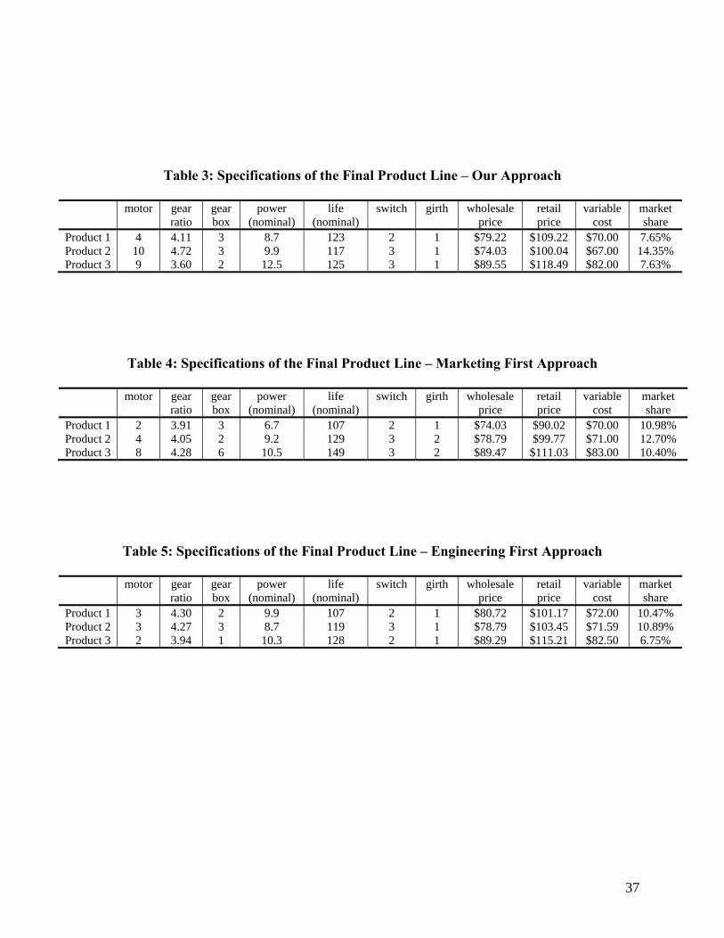
and three products in the product line. The product line with the following specifications
provided the highest earning (see Table 3). We observed that the high earning level of this
product line benefited a great deal from component sharing (the first two products shared the
same gear box type, the last two products used the same switch type, and all three products
consisted of the same girth type). Meanwhile, the product line also exploits the heterogeneous
consumer preferences in the marketplace (see the different power amp, product life, and prices of
these products). Over a five-year horizon, the discounted long-term profit is estimated to be
$52.8 million. We also conducted some robustness checks and found that this final earning level
was not overly sensitive to the parameter specifications of the model (see details in Web
Appendix D).
<Insert Table 3 about here>
Comparison to Benchmark Approaches
We now compare the empirical results obtained from the proposed procedure with two
benchmark approaches in which the marketing and engineering considerations are addressed in a
sequential order. Both approaches comprise two stages. In the marketing-first approach, the
marketing team’s primary goal in the first stage is to search for vectors of consumer attributes
6 The GA parameters used here are the same as the parameters used in the simulation study. We varied the GA parameters several times to evaluate how sensitive the final earning level is to the GA parameters. We also assessed the quality of the solution by using different starting values. No major differences were found in the final earnings.
25
that maximize the product line profitability. The key differences between the optimization at this
stage and the one described in Figure 1 are that: a) the decision variables 111211 ,...,, Lyyy are
replaced by 111211 ,...,, Lxxx and b) the five constraints in the first block of the figure are reduced
to constraints 3) to 5). Because a product’s variable cost is an inherent function of a product’s
design variable configuration and its cost interactions with the other products in the product line,
we had to approximate the product’s cost based on a weighted sum of its attribute levels
(excluding brand and price).7 The other aspects of this optimization are identical to the ones
described in Figure 1. In the second stage, given the consumer attribute specification of each
product in the final product line, the engineering team searches for a combination of design
variables that best match the required values of consumer attributes at the nominal operation
condition. Additionally, the engineering team evaluates whether these design variable
configurations satisfy the engineering feasibility and robustness criteria (the first two constraints
in the first block of Figure 1). If the product violates one or more engineering requirements, the
engineering team will move onto a design variable configuration that produces the second
smallest deviation from the required consumer attribute values. This process continues until all
products satisfy the engineering requirements.
Under this approach, the final product line consisted of three products with the following
specifications (Table 4). The cost and market share estimates in this table are recalibrated using
each product’s actual design variable configurations. As a result of separating marketing and
engineering considerations, this sequential approach led to a sub-optimal product line. In
7 We obtained the weights from a multiple regression using the cost estimates of current products and some hypothetical products. We thank two anonymous reviewers for this suggestion. Additionally, we would like to point out that if the marketing team were able to incorporate cost synergy into the variable cost estimation, the primary advantage of our approach vs. the marketing-first approach hinges on the rigidity of the engineering criteria. If there are a substantial number of engineering requirements, the marketing-first approach may result in a local search in a sub-optimal space. On the other hand, if the vast majority of product candidates satisfy the engineering requirements, the results may not differ much between the proposed and the marketing-first approaches.
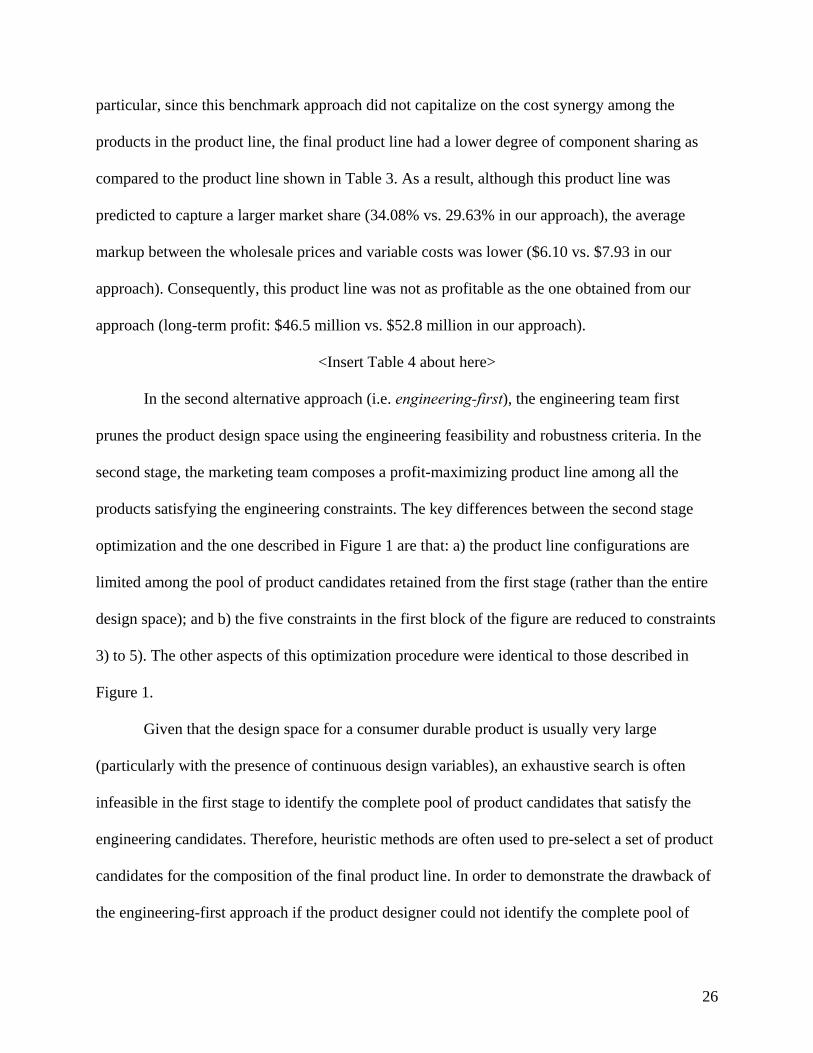
26
particular, since this benchmark approach did not capitalize on the cost synergy among the
products in the product line, the final product line had a lower degree of component sharing as
compared to the product line shown in Table 3. As a result, although this product line was
predicted to capture a larger market share (34.08% vs. 29.63% in our approach), the average
markup between the wholesale prices and variable costs was lower ($6.10 vs. $7.93 in our
approach). Consequently, this product line was not as profitable as the one obtained from our
approach (long-term profit: $46.5 million vs. $52.8 million in our approach).
<Insert Table 4 about here>
In the second alternative approach (i.e. engineering-first), the engineering team first
prunes the product design space using the engineering feasibility and robustness criteria. In the
second stage, the marketing team composes a profit-maximizing product line among all the
products satisfying the engineering constraints. The key differences between the second stage
optimization and the one described in Figure 1 are that: a) the product line configurations are
limited among the pool of product candidates retained from the first stage (rather than the entire
design space); and b) the five constraints in the first block of the figure are reduced to constraints
3) to 5). The other aspects of this optimization procedure were identical to those described in
Figure 1.
Given that the design space for a consumer durable product is usually very large
(particularly with the presence of continuous design variables), an exhaustive search is often
infeasible in the first stage to identify the complete pool of product candidates that satisfy the
engineering candidates. Therefore, heuristic methods are often used to pre-select a set of product
candidates for the composition of the final product line. In order to demonstrate the drawback of
the engineering-first approach if the product designer could not identify the complete pool of

27
product candidates satisfying the engineering criteria in the first stage, we randomly sampled the
design space until obtaining 1,000 products satisfying the engineering criteria. Next, an
exhaustive search was conducted to obtain the profit-maximizing product line when there are 1-3
products in the product line. Table 5 provides the specifications of the most profitable product
line. Because the composition of the final product line was limited to the set of 1,000 products,
some promising product candidates from the marketing perspective may be neglected. Therefore,
although this product line included some degree of component sharing, it was not as profitable as
the one obtained using our approach (profit: $48.3 million vs. $52.8 million in our approach).8
<Insert Table 5 about here>
CONCLUSIONS
In this paper, we introduced a procedure of product line optimization where the
marketing and engineering criteria are considered concurrently in the search for a profit-
maximizing product line. We propose that the product designer needs to take into account both
marketing and engineering considerations concurrently in a product line design. In particular, our
method extends beyond extant methods in product line design by accounting for the strategic
reactions from the competing manufacturers and the retailer in response to the entry of the new
product line. Through a simulation study and an empirical application, we demonstrated that the
proposed optimization procedure provides an effective solution to this challenging problem.
We also contribute to the literature by proposing an optimization method that works in
relatively large-scale design problems consisting of both discrete and continuous design
variables. Particularly, we suggest that genetic algorithm (GA) provides an efficient and effective
8 Note that since the design space in our empirical application is relatively small, we could technically discretize the continuous design variable gear ratio and perform an exhaustive search in the first stage. Under this scenario, the results from the engineering-first approach should be similar to that of ours.
28
solution to the focal manufacturer’s design variable configuration problem in a variety of
problem settings. In contrast, despite of their comparable performance in finding profit-
maximizing product lines, the heuristic method of simulated annealing (SA) is only suitable for
small-scale problems (given its computational inefficiency) and the decompositional method of
analytical target cascading (ATC) is applicable to problems with only continuous design
variables.
Our research is not without limitations. First, the proposed method is built upon the
assumption that the product designer has complete knowledge about the various inputs needed
for the optimization. Therefore, exploratory research will be needed if some inputs are unknown.
Second, because the product line design problem is NP-hard, our optimization procedure may
recover a local maximum rather than a global maximum. Future research may investigate
optimization methods that can guarantee a global optimality. Third, although accounting for the
retailer and the incumbent’s strategic price reactions, our method is limited in addressing the
incumbents’ strategic responses in non-price attributes. Finally, because our optimization method
is combinatorial by nature, firms facing extremely large problems may encounter computational
difficulty. Future research may develop a decompositional approach that handles both discrete
and continuous design variables. In time, as both the algorithm and computational power
improve, further research may be able to extend our work by guaranteeing global optimality in a
considerably large scale product line design problem.
References
Balakrishnan, P.V., Rakesh Gupta, Varghese S. Jacob (2004), “Development of Hybrid Genetic
Algorithms for Product Line Designs”, IEEE Transactions on Systems, Man, and
Cybernetics – Part B: Cybernetics, Vol. 34, No. 1, 468-483.

29
Balakrishnan, P.V., Rakesh Gupta, Varghese S. Jacob (2006), “An Investigation of Mating and
Population Maintenance Strategies in Hybrid Genetic Heuristics for Product Line
Designs”, Computer & Operations Research, Vol.33, Issue 3, 639-659.
Belloni, Alexandre, Robert Freund, Matthew Selove, and Duncan Simester (2008), “Optimizing
Product Line Designs: Efficient Methods and Comparisons”, Management Science,
Vol.54, No.9, 1544-1552.
Besharati, Babak, Lan Luo, Shapour Azarm, and P. K. Kannan (2004), “An Integrated Robust
Design and Marketing Approach for Product Design Selection Process”, ASME IDETC
2004 Proceedings, Salt Lake City, UT.
Besharati, Babak, Lan Luo, Shapour Azarm, and P. K. Kannan (2006), “Multi-Objective Single
Product Robust Optimization: An Integrated Design and Marketing Approach”, ASME
Journal of Mechanical Design, Vol. 128, No. 4, 884-892.
Chen, Kyle D. and Warren H. Hausman (2000), “Mathematical Properties of the Optimal
Product Line Selection Problem using Choice-Based Conjoint Analysis”, Management
Science, Vol. 46, No. 2, 327-332.
Dobson, Gregory and Shlomo Kalish (1988), “Positioning and Pricing a Product Line”,
Marketing Science, Vol. 7, No. 2, 107-125.
Dobson, Gregory and Shlomo Kalish (1993), “Heuristics for Pricing and Positioning a Product-
line using Conjoint and Cost Data”, Management Science, Vol. 39, No. 2, 1993.
D’Souza, Bryan and Timothy W. Simpson (2003), “A Genetic Algorithm Based Method for
Product Family Design Optimization”, Engineering Optimization, Vol. 35, No. 1, 1-18.

30
Farrell, Ronald S. and Timothy W. Simpson (2003), “Product Platform Design to Improve
Commonality in Custom Products”, Journal of Intelligent Manufacturing, Vol.14, No.6,
541-556.
Farrell, Ronald S. and Timothy W. Simpson (2009), “Improving cost effectiveness in an existing
product line using component product platforms”, International Journal of Production
Research, Published Online May 2009.
Gordon, Brett (2009), “A Dynamic Model of Consumer Replacement Cycles in the PC Processor
Industry”, forthcoming, Marketing Science.
Green, Paul E. and Abba M. Krieger (1985), “Models and Heuristics for Product Line Selection”,
Marketing Science, Vol. 4, No. 1, 1-19.
Griffin, Abbie and John R. Hauser (1993), “The Voice of the Customer”, Marketing Science, Vol.
12, No. 1, 1-27.
Hanson, Ward and Kipp Martin (1996), “Optimizing Multinomial Logit Profit Functions”,
Management Science, Vol. 42, No. 7, 992-1003.
Hauser, John R. (1988), “Competitive Price and Pricing Strategies”, Marketing Science, Vol.7,
No.1, 76-91.
Hauser, John R. and Clausing, D. (1988), “The House of Quality”, Harvard Business Review,
Vol.3, 63-73.
Hauser, John R., Gerard J. Tellis, and Abbie Griffin (2006), “Research on Innovation: A Review
and Agenda for Marketing Science”, Marketing Science, Vol.25, No.6, 687-717.
Heese, Hans S. and Jayashankar M. Swaminathan (2006), “Product Line Design with
Component Commonality and Cost-Reduction Effort”, Manufacturing & Service
Operations Management, Vol. 8, No.2, 206-219.
31
Jiao, Jianxin and Yiyang Zhang (2005), “Product Portfolio Planning with Customer-Engineering
Interaction”, IIE Transactions, Vol. 37, No.9, 801-814.
Kalsi, Monu, Kurt Hacker, and Kemper Lewis (2001), “A Comprehensive Robust Design
Approach for Decision Trade-Offs in Complex Systems Design”, ASME Journal of
Mechanical Design, Vol. 123, No. 1, 1-10.
Kannan, P.K., Barbara K. Pope, and Sanjay Jain (2009), “Pricing Digital Content Product Lines:
A Model and Application for the National Academies Press”, Marketing Science, Vol. 28,
No. 4, 620-636.
Kaul, Anil and Vithala R. Rao (1995), “Research for Product Positioning and Design Decisions:
An Integrative Review”, Internal Journal of Research in Marketing, Vol. 12, No.4, 293-
320.
Kohli, Rajeev and R. Sukumar (1990), “Heuristics for Product-Line Design using Conjoint
Analysis”, Management Science, Vol. 36, No.12, 1464-1478.
Kouvelis, Panos and Yu, G. (1997), Robust Discrete Optimization and Its Applications, Kluwer
Academic Publishers, Dordrecht, Netherlands.
Kumar, Deepak, Wei Chen, and Timothy W. Simpson (2009), “A Market-Driven Approach to
the Design of Platform-Based Product Families”, International Journal of Production
Research, Vol. 47, No. 1, 71-104.
Li, Hui, and Shapour Azarm (2000), “Product design selection under uncertainty and with
competitive advantage”, ASME Journal of Mechanical Design, Vol. 122, No. 4, 411-418.
Li, Hui, and Shapour Azarm (2002), “An Approach for Product Line Design Selection under
Uncertainty and Competition”, ASME Journal of Mechanical Design, Vol. 124, No. 3,
385-392.
32
Luo, Lan, P.K. Kannan, Babak Besharati, and Shapour Azarm (2005), “Design of Robust New
Products under Variability: Marketing Meets Design”, Journal of Product Innovation
Management, Vol. 22, No. 2, 177-192.
Luo, Lan, P.K. Kannan, and Brian T. Ratchford (2007), “New Product Development Under
Channel Acceptance”, Marketing Science, Vol. 26, No. 2, 149-163.
McBride, Richard D. and Fred S. Zufryden (1988), “An Integer Programming Approach to the
Optimal Product Line Selection Problem”, Marketing Science, Vol. 7, No. 2, 126-140.
Michalek, Jeremy J., Oben Ceryan, Panos Y. Papalambros, and Yoram Koren (2006),
“ Balancing Marketing and Manufacturing Objectives in Product Line Design”, ASME
Journal of Mechanical Design, Vol. 128, No. 6, 1196-1204.
Michalek, Jeremy J., Fred M. Feinberg, and Panos Y. Papalambros (2005), “Linking Marketing
and Engineering Product Design Decisions via Analytical Target Cascading”, Journal of
Product Innovation Management, Vol. 21, No. 1, 42-62.
Michalek, Jeremy J., Fred M. Feinberg, Peter Ebbes, Feray Adigüzel, and Panos Y. Papalambros
(2009), “Optimal Feasible Product Design for Heterogenous Markets”, working paper.
Moore, William L, Jordan J. Louviere and Rohit Verma (1999), “Using Conjoint Analysis to
Help Design Product Platforms”, Journal of Product Innovation Management, Vol.16,
27-39.
Morgan, Leslie O., Richard L. Daniels, and Panos Kouvelis (2001), “Marketing/Manufacturing
Trade-Offs in Product Line Management”, IIE Transactions, Vol. 33, No. 11, 949-962.
Nair, Suresh K, Lakshman S. Thakur, and Kuang-Wei Wen (1995), “Near Optimal Solutions for
Product Line Design and Selection: Beam Search Heuristics”, Management Science, Vol.
41, No. 5, 767-785.
33
Quiggin, John (1982), “A Theory of Anticipated Utility”, Journal of Economic Behavior and
Organization, Vol. 3, 323-343.
Rai, Rahul and Venkat Allada (2006), “Agent-based Optimization for Product Family Design”,
Annals of Operations Research, Vol.143, No.1, 147-156.
Ramdas, Kamalini and Mohanbir S. Sawhney (2001), “A Cross-Functional Approach to
Evaluating Multiple Line Extensions for Assembled Products”, Management Science,
Vol. 47, No. 1, 22-36.
Rossi, Peter E. and Greg M. Allenby (2003), “Bayesian Statistics and Marketing”, Marketing
Science, Vol. 22, No. 3, 304-328.
Sawtooth Choice-Based Conjoint User Manual (2001), Sawtooth Software Inc., Sequim, WA. Simpson, Timothy W. (2004), “Product Platform Design and Customization: Status and
Promise”, Artificial Intelligence for Engineering Design, Analysis and Manufacturing,
Vol. 18, No.1, 3-20.
Simpson, Timothy W., Carolyn Conner Seepersad, and Farrokh Mistree (2001), “Balancing
Commonality and Performance within the Concurrent Design of Multiple Products in a
Product Family”, Concurrent Engineering: Research and Applications, Vol. 0, No. 0, 1-
14.
Srinivasan, V., William S. Lovejoy, and David Beach (1997), “Integrated Product Design for
Marketability and Manufacturing”, Journal of Marketing Research, Vol. 34, No. 1, 154-
163.
Steiner, Winfried and Harald Hruschka (2003), “Genetic Algorithms for Product Design: How
Well Do They Really Work?”, International Journal of Market Research, Vol. 45,
Quarter 2, 229-240.

34
Tarasewich, Peter and Patrick R. McMullen (2001), “A Pruning Heuristic for Use with
Multisource Product Design”, European Journal of Operational Research, Vol.128, 58-
73.
Tarasewich, Peter and Suresh K. Nair (2001), “Designer-Moderated Product Design”, IEEE
Transactions On Engineering Management, Vol. 48, No.2, 175-188.
Ulrich, Karl T. and Steven D. Eppinger (2004), Product Design and Development, McGraw-
Hill/Irwin Publishing, New York.
35
Figure 1: Computational Procedure of the Product Line Optimization
k
T
t
L
l
ttklklkl
mk
wwwFrDmcw
k
kkLkk
1 1,...,,
1/**)(max21
01
012
,011
01
012
,011 11
,...,,,,...,, LL pppwww
),...,,,,...,,( *1
*12
*11
*1
*12
*11 11 LL wwwyyy
(w11 ,w
12 ,…,w
1L1 ), (p
11 ,p12 ,…
,p1L
1 )
111211 ,...,, Lyyy
0
1012
011
01
012
011
1
1
,...,,
,...,,
L
L
pwp
www
Initialize wholesale and retail prices for each product
in the product line
Search for design variable configurations to maximize
product line profit
111211 ,..., Lyyy
Adjust wholesale and retail prices for the new product
line and incumbent products
(w11 ,w
12 ,…,w
1L1),
(p11 ,p
12 ,…,p
1L1),
The Final Product Line
The focal manufacturer’s design variable configuration problem
)acceptance (retailer
length)line product maximum
capacity
,1,
robustness
ty)(feasibili
rr
ltl
UPLW
Jblblb
UPLW
H
hlh
T
t
L
lL
ttlll
m
LL
TtLlwithWDm
LlBbwith
fff
Llwith
gts
FrDmvcwL
)5
()4
)(,...,1;,...,1*)3
,...,1;;
)(),(),((max)2
,...,1;
0)],(,0max[)1..
1/**max
11
111
1
011
1
11
1 111111
,...,,
1
1111211
papapa
paypay
papapa
pay
yyy
The retailer and manufacturer’s price adjustment problem
k
T
t
L
l
ttklklkl
mk
wwwFrDmcw
k
kkLkk
1 1,...,,
1/**)(max21
K
kk
T
t
K
k
L
l
ttklklkl
r
ppppLscrDwpm
k
KKLKL 11 1 1,...,,...,,...,
1/)(*max11111
k=1,…, K

36
Table 1: Algorithm Comparisons for the Focal Manufacturer’s
Design Variable Configuration Problem (First Block of Figure 1)
Note: the average profits are presented in millions and the average CPU time is presented in seconds.
Table 2: Bayesian Finite Mixture Conjoint Part-worth Estimates
Segment 1 Segment 2
Segment Size 0.147 0.853
Posterior Part-worth Mean SD* Mean SD Own Brand 0.859 0.857 0.164 0.205 Brand 1 1.077 0.533 -0.299 0.270 Brand 2 2.233 1.139 0.298 0.268 Brand 3 -4.169 1.885 -0.163 0.362
Price (mean-centered) -0.342 0.181 -0.044 0.517
Power amp: 6 -1.630 0.577 -0.318 0.412 Power amp: 9 0.240 0.376 0.090 0.427 Power amp: 12 1.390 0.434 0.228 0.603
Product Life: 80 hrs -3.682 1.636 -0.334 0.476 Product Life: 110 hrs -1.346 1.602 0.028 0.525 Product Life: 150 hrs 5.028 1.436 0.306 0.584
Switch type 1: paddle -1.503 0.661 -0.333 0.588 Switch type 2: top slider 1.966 0.676 0.320 0.485 Switch type 3: side slider 0.593 0.565 0.517 0.305 Switch type 4: trigger -1.056 0.608 -0.504 0.414
Girth type 1: small 1.173 1.006 -0.035 0.180 Girth type 2: large -1.173 1.006 0.035 0.180
No-Choice - - 0.477 0.211
*These entries are the posterior estimates of the square roots of the diagonal terms in the variance-covariance matrix (i.e. sΩ ). They represent the degree of heterogeneity within each consumer segment.
Number of products
Mix of discrete & continuous variables Continuous variables only
GA SA GA SA ATC
Ave Profit
Ave CPU time
Ave profit
Ave CPU time
Ave profit
Ave CPU time
Ave profit
Ave CPU time
Ave profit
Ave CPU time
Small (1-3) 65.5 0.9 63.9 29.0 68.8 1.1 68.1 40.8 69.0 0.9 Medium (4-5) 105.2 1.2 107.8 78.8 103.2 1.3 105.1 117.5 104.7 2.3
Large (6-8) 92.2 1.8 90.9 195.7 87.4 1.9 88.6 232.9 90.5 3.6
37
Table 3: Specifications of the Final Product Line – Our Approach
motor gear ratio
gear box
power (nominal)
life (nominal)
switch girth wholesale price
retail price
variable cost
market share
Product 1 4 4.11 3 8.7 123 2 1 $79.22 $109.22 $70.00 7.65% Product 2 10 4.72 3 9.9 117 3 1 $74.03 $100.04 $67.00 14.35% Product 3 9 3.60 2 12.5 125 3 1 $89.55 $118.49 $82.00 7.63%
Table 4: Specifications of the Final Product Line – Marketing First Approach
motor gear ratio
gear box
power (nominal)
life (nominal)
switch girth wholesale price
retail price
variable cost
market share
Product 1 2 3.91 3 6.7 107 2 1 $74.03 $90.02 $70.00 10.98% Product 2 4 4.05 2 9.2 129 3 2 $78.79 $99.77 $71.00 12.70% Product 3 8 4.28 6 10.5 149 3 2 $89.47 $111.03 $83.00 10.40%
Table 5: Specifications of the Final Product Line – Engineering First Approach
motor gear ratio
gear box
power (nominal)
life (nominal)
switch girth wholesale price
retail price
variable cost
market share
Product 1 3 4.30 2 9.9 107 2 1 $80.72 $101.17 $72.00 10.47% Product 2 3 4.27 3 8.7 119 3 1 $78.79 $103.45 $71.59 10.89% Product 3 2 3.94 1 10.3 128 2 1 $89.29 $115.21 $82.50 6.75%