Producer Theory - Gies College of Business - University of ... · PDF fileProducer Theory...
37
Chapter 5 Producer Theory Markets have two sides: consumers and producers. Up until now we have been studying the consumer side of the market. We now begin our study of the producer side of the market. The basic unit of activity on the production side of the market is the firm. The task of the firm is take commodities and turn them into other commodities. The objective of the firm (in the neoclassical model) is to maximize profits. That is, the firm chooses the production plan from among all feasible plans that maximizes the profit earned on that plan. In the neoclassical (competitive) production model, the firm is assumed to be one firm among many others. Because of this (as in the consumer model), prices are exogenous in the neoclassical production model. Firms are unable to affect the prices of either their inputs or their outputs. Situations where the firm is able to affect the price of its output will be studied later under the headings of monopoly and oligopoly. Our study of production will be divided into three parts: First, we will consider production from a purely technological point of view, characterizing the firm’s set of feasible production plans in terms of its production set Y . Second, we will assume that the firm produces a single output using multiple inputs, and we will study its profit maximization and cost minimization problems using a production function to characterize its production possibilities. Finally, we will consider a special class of production models, where the firm’s production function exhibits constant returns to scale. 121
Transcript of Producer Theory - Gies College of Business - University of ... · PDF fileProducer Theory...
Chapter 5
Producer Theory
Markets have two sides: consumers and producers. Up until now we have been studying the
consumer side of the market. We now begin our study of the producer side of the market.
The basic unit of activity on the production side of the market is the firm. The task of the
firm is take commodities and turn them into other commodities. The objective of the firm (in
the neoclassical model) is to maximize profits. That is, the firm chooses the production plan
from among all feasible plans that maximizes the profit earned on that plan. In the neoclassical
(competitive) production model, the firm is assumed to be one firm among many others. Because
of this (as in the consumer model), prices are exogenous in the neoclassical production model.
Firms are unable to affect the prices of either their inputs or their outputs. Situations where the
firm is able to affect the price of its output will be studied later under the headings of monopoly
and oligopoly.
Our study of production will be divided into three parts: First, we will consider production
from a purely technological point of view, characterizing the firm’s set of feasible production plans
in terms of its production set Y . Second, we will assume that the firm produces a single output
using multiple inputs, and we will study its profit maximization and cost minimization problems
using a production function to characterize its production possibilities. Finally, we will consider a
special class of production models, where the firm’s production function exhibits constant returns
to scale.
121

Nolan Miller Notes on Microeconomic Theory: Chapter 5 ver: Aug. 2006
5.1 Production Sets
Consider an economy with L commodities. The task of the firm is to change inputs into outputs.
For example, if there are three commodities, and the firm uses 2 units of commodity one and
3 units of commodity two to produce 7 units of commodity three, we can write this production
plan as y = (−2,−3, 7), where, by convention, negative components mean that that commodity is
an input and positive components mean that that commodity is an output. If the prices of the
three commodities are p = (1, 2, 2), then a firm that chooses this production plan earns profit of
π = p · y = (1, 2, 2) · (−2,−3, 7) = 6.
Usually, we will let y = (y1, ..., yL) stand for a single production plan, and Y ⊂ RL stand for
the set of all feasible production plans. The shape of Y is going to be driven by the way in which
different inputs can be substituted for each other in the production process.
A typical production set (for the case of two commodities) is shown in MWG Figure 5.B.1.
The set of points below the curved line represents all feasible production plans. Notice that in this
situation, either commodity 1 can be used to produce commodity 2 (y1 < 0, y2 > 0), commodity
2 can be used to produce commodity 1 (y1 > 0, y2 < 0), nothing can be done (y1 = y2 = 0) or
both commodities can be used without producing an output, (y1 < 0, y2 < 0). Of course, the last
situation is wasteful — if it has the option of doing nothing, then no profit-maximizing firm would
ever choose to use inputs and incur cost without producing any output. While this is true, it is
useful for certain technical reasons to allow for this possibility.
Generally speaking, it will not be profit maximizing for the firm to be wasteful. What is meant
by wasteful? Consider a point y inside Y in Figure 5.B.1. If y is not on the northeast frontier
of Y then it is wasteful. Why? Because if this is the case the firm can either produce more
output using the same amount of input or the same output using less input. Either way, the firm
would earn higher profit. Because of this it is useful to have a mathematical representation for the
frontier of Y . The tool we have for this is called the transformation function, F (y) , and we
call the northeast frontier of the production set the production frontier. The transformation
function is such that
F (y) = 0 if y is on the frontier
< 0 if y is in the interior of Y
> 0 if y is outside of Y .
Thus the transformation function implicitly defines the frontier of Y . Thus if F (y) < 0, y represents
122

Nolan Miller Notes on Microeconomic Theory: Chapter 5 ver: Aug. 2006
some sort of waste, although F () tells us neither the form of the waste nor the magnitude.
The transformation function can be used to investigate how various inputs can be substituted
for each other in the production process. For example, consider a production plan y such that
F (y) = 0. The slope of the transformation frontier with respect to commodities i and j is given
by:∂yi∂yj
= −Fj (y)Fi (y)
.
The absolute value of the right-hand side of this expression, Fj(y)Fi(y), is known as the marginal rate
of transformation of good j for good i at y (MRTji).
MRTji =Fj (y)
Fi (y)
It tells how much you must increase the (net) usage of factor j if you decrease the net usage
of factor i in order to remain on the transformation frontier. It is important to note that factor
usage can be either positive or negative in this model. In either case, increasing factor usage means
moving to the right on the number line. Thus if you are using −5 units of an input, going to −4
units of that input is an increase, as far as the MRT is concerned.
For example, suppose we are currently at y = (−2, 7) , that F (−2, 7) = 0, and that we are
interested in MRT12, the marginal rate of transformation of good 1 for good 2. MRT12 =F1(−2,7)F2(−2,7) .
Now, if the net usage of good 1 increases, say from −2 to −1, then we move out of the production
set, and F (−1, 7) > 0. Hence F1 (−2, 7) > 0. If we increase commodity 3 a small amount, say to
8, we also move out of the production set, and F (−2, 8) > 0. So, MRT12 > 0.
The slope of the transformation frontier asks how much the net usage of factor 2 must be
changed if the net usage of factor 1 is increased. Thus it is a negative number. This is why the
slope of the transformation frontier is negative when comparing an input and an output, but the
MRT is positive.
5.1.1 Properties of Production Sets
There are a number of properties that can be attributed to production sets. Some of these will be
assumed for all production sets, and some will only apply to certain production sets.
Properties of All Production Sets
Here, I will list properties that we assume all production sets satisfy.
123
Nolan Miller Notes on Microeconomic Theory: Chapter 5 ver: Aug. 2006
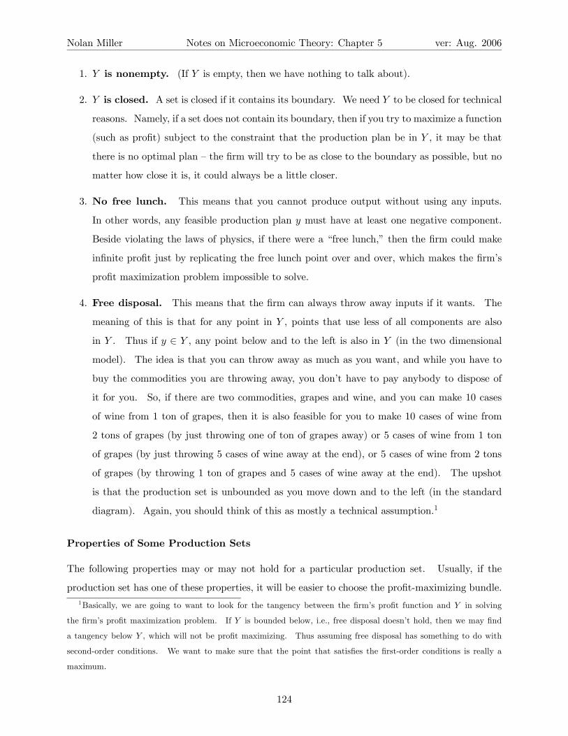
1. Y is nonempty. (If Y is empty, then we have nothing to talk about).
2. Y is closed. A set is closed if it contains its boundary. We need Y to be closed for technical
reasons. Namely, if a set does not contain its boundary, then if you try to maximize a function
(such as profit) subject to the constraint that the production plan be in Y , it may be that
there is no optimal plan — the firm will try to be as close to the boundary as possible, but no
matter how close it is, it could always be a little closer.
3. No free lunch. This means that you cannot produce output without using any inputs.
In other words, any feasible production plan y must have at least one negative component.
Beside violating the laws of physics, if there were a “free lunch,” then the firm could make
infinite profit just by replicating the free lunch point over and over, which makes the firm’s
profit maximization problem impossible to solve.
4. Free disposal. This means that the firm can always throw away inputs if it wants. The
meaning of this is that for any point in Y , points that use less of all components are also
in Y . Thus if y ∈ Y , any point below and to the left is also in Y (in the two dimensional
model). The idea is that you can throw away as much as you want, and while you have to
buy the commodities you are throwing away, you don’t have to pay anybody to dispose of
it for you. So, if there are two commodities, grapes and wine, and you can make 10 cases
of wine from 1 ton of grapes, then it is also feasible for you to make 10 cases of wine from
2 tons of grapes (by just throwing one of ton of grapes away) or 5 cases of wine from 1 ton
of grapes (by just throwing 5 cases of wine away at the end), or 5 cases of wine from 2 tons
of grapes (by throwing 1 ton of grapes and 5 cases of wine away at the end). The upshot
is that the production set is unbounded as you move down and to the left (in the standard
diagram). Again, you should think of this as mostly a technical assumption.1
Properties of Some Production Sets
The following properties may or may not hold for a particular production set. Usually, if the
production set has one of these properties, it will be easier to choose the profit-maximizing bundle.1Basically, we are going to want to look for the tangency between the firm’s profit function and Y in solving
the firm’s profit maximization problem. If Y is bounded below, i.e., free disposal doesn’t hold, then we may find
a tangency below Y , which will not be profit maximizing. Thus assuming free disposal has something to do with
second-order conditions. We want to make sure that the point that satisfies the first-order conditions is really a
maximum.
124
Nolan Miller Notes on Microeconomic Theory: Chapter 5 ver: Aug. 2006
1. Irreversibility. Irreversibility says that the production process cannot be undone. That
is, if y ∈ Y and y 6= 0, then −y /∈ Y . Actually, the laws of physics imply that all production
processes are irreversible. You may be able to turn gold bars into jewelry and then jewelry
back into gold bars, but in either case you use energy. So, this process is not really reversible.
The reason why I call this a property of some production sets is that, even though it is true
of all real technologies, we often do not need to invoke irreversibility in order to get the
results we are after. And, since we don’t like to make assumptions we don’t need, in many
cases it won’t be stated. On the other hand, you should beware of results that hinge on the
reversibility of a technology, for the physics reasons I mentioned earlier.
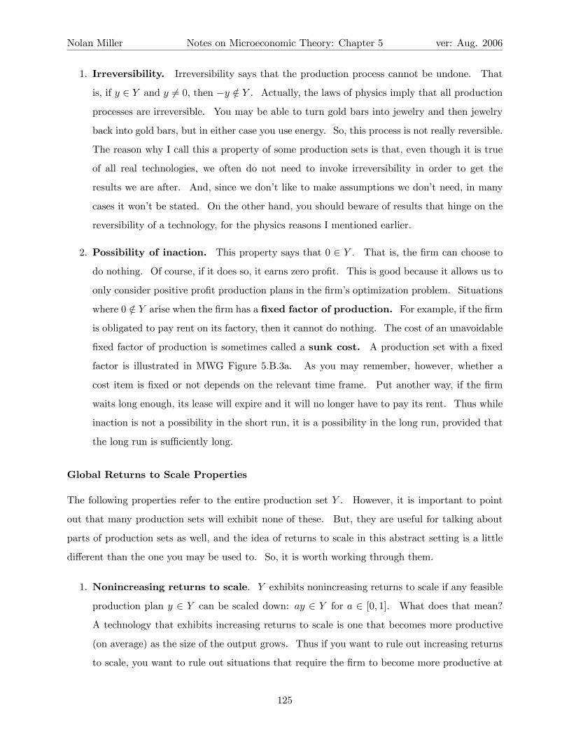
2. Possibility of inaction. This property says that 0 ∈ Y . That is, the firm can choose to
do nothing. Of course, if it does so, it earns zero profit. This is good because it allows us to
only consider positive profit production plans in the firm’s optimization problem. Situations
where 0 /∈ Y arise when the firm has a fixed factor of production. For example, if the firm
is obligated to pay rent on its factory, then it cannot do nothing. The cost of an unavoidable
fixed factor of production is sometimes called a sunk cost. A production set with a fixed
factor is illustrated in MWG Figure 5.B.3a. As you may remember, however, whether a
cost item is fixed or not depends on the relevant time frame. Put another way, if the firm
waits long enough, its lease will expire and it will no longer have to pay its rent. Thus while
inaction is not a possibility in the short run, it is a possibility in the long run, provided that
the long run is sufficiently long.
Global Returns to Scale Properties
The following properties refer to the entire production set Y . However, it is important to point
out that many production sets will exhibit none of these. But, they are useful for talking about
parts of production sets as well, and the idea of returns to scale in this abstract setting is a little
different than the one you may be used to. So, it is worth working through them.
1. Nonincreasing returns to scale. Y exhibits nonincreasing returns to scale if any feasible
production plan y ∈ Y can be scaled down: ay ∈ Y for a ∈ [0, 1]. What does that mean?
A technology that exhibits increasing returns to scale is one that becomes more productive
(on average) as the size of the output grows. Thus if you want to rule out increasing returns
to scale, you want to rule out situations that require the firm to become more productive at
125

Nolan Miller Notes on Microeconomic Theory: Chapter 5 ver: Aug. 2006
higher levels of production. The way to do this is to require that any feasible production
plan y can be scaled down to ay, for a ∈ [0, 1]. If this holds, then the feasibility of y does not
depend on the fact that it involves a large scale of production and the firm gets more efficient
at large scale.
2. Nondecreasing returns to scale. Y exhibits nondecreasing returns to scale if any feasible
production plan y ∈ Y can be scaled up: ay ∈ Y for a ≥ 1. Decreasing returns to scale
is a situation where the firm grows less productive at higher levels of output. Thus if we
want to rule out the case of decreasing returns to scale, we must rule out the case where y
is feasible, but if that same production plan were scaled larger to ay, it would no longer be
feasible because the firm is less productive at the higher scale. Thus we require that ay ∈ Y
for a ≥ 1.
• Note that if a firm has fixed costs, it may exhibit nondecreasing returns to scale but
cannot exhibit nonincreasing returns to scale. See MWG Figure 5.B.6.
3. Constant returns to scale. Y exhibits constant returns to scale if it exhibits both non-
increasing returns to scale and non-decreasing returns to scale at all y. That is, for all
a ≥ 0, if y ∈ Y , then ay ∈ Y. Constant returns to scale means that the firm’s productivity is
independent of the level of production. Thus it means that any feasible production plan can
either be scaled upward or downward.
• Constant returns to scale implies the possibility of inaction.
4. Convexity. If Y exhibits nonincreasing returns to scale, then Y is convex.
Note that the list of returns to scale properties is by no means exhaustive. In fact, most
real technologies exhibit none of these. The “typical” technology that we think of is one that
at first exhibits increasing returns to scale, and then exhibits decreasing returns to scale. This
would be the case, for example, for a manufacturing firm whose factory size is fixed. At first,
as output increases, its average productivity increases as it spreads the factory cost over more
output. However, eventually the firm’s output becomes larger than the factory is designed for. At
this point, the firm’s average productivity falls as the workers become crowded, machines become
overworked, etc. A typical example of this type of technology is illustrated in MWG Figure 5.F.2.
126

Nolan Miller Notes on Microeconomic Theory: Chapter 5 ver: Aug. 2006
So, while the previous definitions were global, we can also think of local versions. A technology
exhibits nonincreasing returns at a point on the transformation frontier if the transformation frontier
is locally concave there, and it exhibits nondecreasing returns at a point if the transformation
function is locally convex there. Also note, decreasing returns to scale means that returns are
nonincreasing and not constant — thus the transformation frontier is locally strictly concave. The
opposite goes for increasing returns — the transformation frontier is locally strictly convex.
5.1.2 Profit Maximization with Production Sets
As we said earlier, the firm’s objective is to maximize profit. Using the production plan approach we
outlined earlier, the profit earned on production plan y is p·y. Hence the firm’s profit maximization
problem (PMP) is given by:
maxy
p · y
s.t. y ∈ Y.
Since Y = {y|F (y) ≤ 0}, this problem can be rewritten as:
maxy
p · y
s.t. : F (y) ≤ 0.
If F () is differentiable, this problem can be solved using standard Lagrangian techniques. The
graphical solution to this problem is depicted in Figure 5.1. The Lagrangian is:
L = p · y − λF (y)
which implies first-order conditions:
pi = λFi (y∗) , for i = 1, ..., L
F (y∗) ≤ 0.
As before, we can solve the first-order conditions for goods i and j in terms of λ and set them
equal, yielding:
piFi (y∗)
= λ =pj
Fj (y∗)
Fi (y∗)
Fj (y∗)=
pipj. (5.1)
127

Nolan Miller Notes on Microeconomic Theory: Chapter 5 ver: Aug. 2006
F(y) = 0
p.y = constant
y*
y2
y1
Figure 5.1: The Profit Maximization Problem
Also, since we established that points strictly inside Y are wasteful, and wasteful behavior is not
profit maximizing, we know that the constraint will bind. Hence F (y∗) = 0.
Condition 5.1 is a tangency condition, similar to the one we derived in the consumer’s problem.
It says that at the profit maximizing production plan y∗, the marginal rate of transformation
between any two commodities is equal to the ratio of their prices.
Figure 5.1 presents the PMP. The profit isoquant is a downward sloping line with slope −p1p2.
We move the profit line up and to the right until we find the point of tangency. This is the point
that satisfies the optimality condition 5.1. Note that unless Y is convex, the first-order conditions
will not be sufficient for a maximum. Generally, second-order conditions will need to be checked.
This can be seen in Figure 5.1, since there is a point of tangency that is not a maximum.
The solution to the profit maximization problem, y (p), is called the firm’s net supply function.
The value function for the profit maximization problem, π (p) = p · y (p), is called the profit
function.2
One thing to worry about is whether this solution exists. When Y is strictly convex and the
production frontier becomes sufficiently flat (i.e., the firm experiences strongly decreasing returns)
at some high level of production, it is not too hard to show that a solution exists.
Problems can arise when the firm’s production set is not convex, i.e., its technology exhibits
nondecreasing returns to scale. In this case, the production frontier is convex.3 If you go through
the graphical analysis we did earlier, you’ll discover that if the firm maximizes profit, it either
produces nothing at all (if the output price is small relative to the input price), or else it can
2There is a direct correspondence to consumer theory. y (p) is like x (p, w), and π (p) is like v (p,w).3Again, remember the distinction between a convex set and a convex function.
128
Nolan Miller Notes on Microeconomic Theory: Chapter 5 ver: Aug. 2006
always increase profit by moving further out on its production frontier. Thus its production
becomes infinite, as do its profits. This problem also arises when the firm’s production function
exhibits increasing returns to scale only over a region of its transformation frontier. It is fairly
straightforward to show that the firm’s profit maximizing point will never be on a part of the
production frontier exhibiting increasing returns (formally, because the second order conditions
will not hold). As a result, we will focus most of our attention on technologies that exhibit
nonincreasing returns.
5.1.3 Properties of the Net Supply and Profit Functions
Just like the demand functions and indirect utility functions from consumer theory, the net supply
function and profit function also have many properties worth knowing.
Let Y be the firm’s production set, and suppose y (p) solves the firm’s profit maximization
problem. Let π (p) = p · y (p) be the associated profit function. The net supply function y (p) has
the following properties:
1. y (p) is homogeneous of degree zero in p. The reason for this is the same as always.
The optimality conditions for the PMP involve a tangency condition, and tangencies are not
affected by re-scaling all prices by the same amount.
2. If Y is convex, y (p) is a convex set. If Y is strictly convex, then y (p) is a single
point. The reason for this is the same as in the UMP. But, notice that while it made sense
to think of utility as being quasiconcave, it is not always reasonable to think of Y as being
convex. Recall that a convex set Y corresponds to non-increasing returns. But, many real
productive processes exhibit increasing returns, at least over some range. So, the convexity
assumption rules out more important cases in profit maximization than quasiconcavity did
in the consumer problem.
The profit function π (p) has the following properties:
1. π (p) is homogenous of degree 1 in p. Again, the reason for this is the same as the
reason why h (p, u) is homogenous of degree zero but e (p, u) is homogeneous of degree 1.
π (p) = p · y (p). π (ap) = ap · y (ap) = ap · y (p) = aπ (p). Since scaling all prices by a > 0
does not change relative prices, the optimal production plan does not change. However,
multiplying all prices by a multiplies profit by a as well. Thus profit is homogenous of degree
1.
129
Nolan Miller Notes on Microeconomic Theory: Chapter 5 ver: Aug. 2006
p p’ price
Price of Output Increases profitp
rearrange plan
don’t rearrange plan
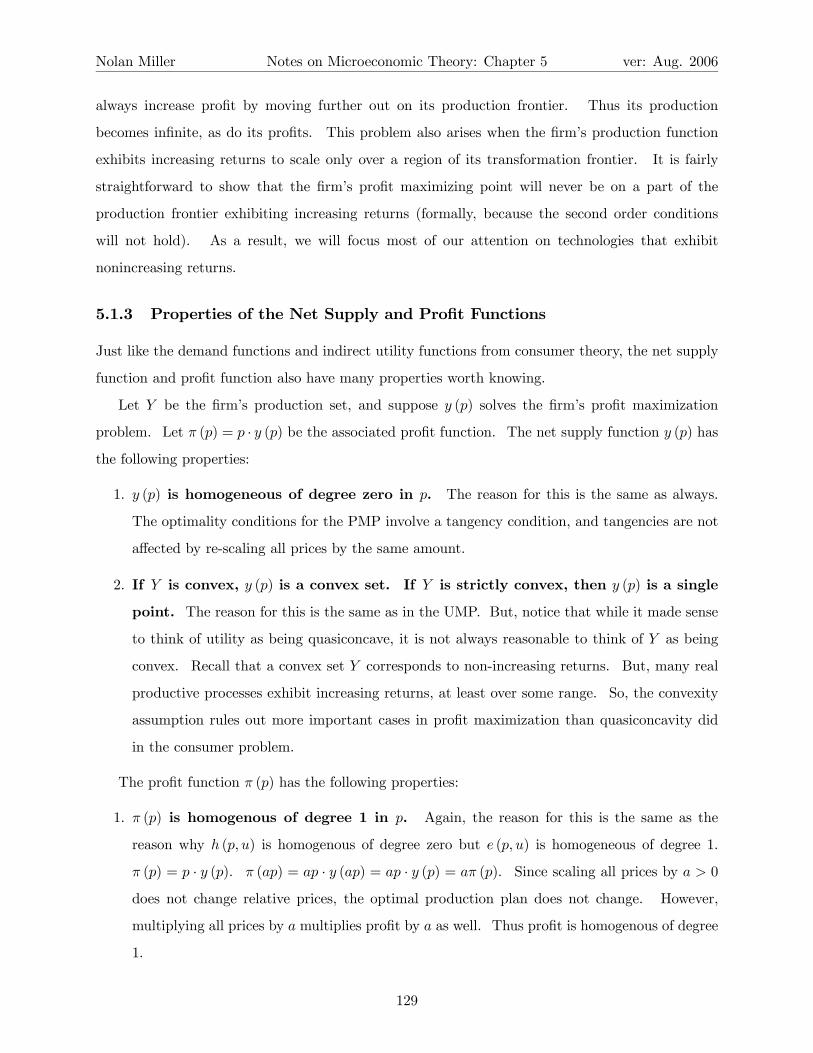
Figure 5.2: Convexity of π (p)
p p’ price
Price of Input Increases
rearrange plan
don’t rearrange plan
profitp
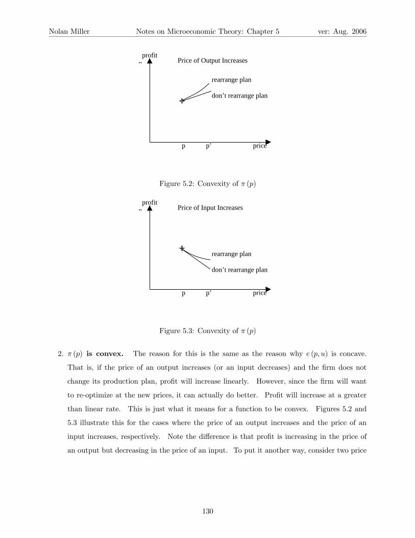
Figure 5.3: Convexity of π (p)
2. π (p) is convex. The reason for this is the same as the reason why e (p, u) is concave.
That is, if the price of an output increases (or an input decreases) and the firm does not
change its production plan, profit will increase linearly. However, since the firm will want
to re-optimize at the new prices, it can actually do better. Profit will increase at a greater
than linear rate. This is just what it means for a function to be convex. Figures 5.2 and
5.3 illustrate this for the cases where the price of an output increases and the price of an
input increases, respectively. Note the difference is that profit is increasing in the price of
an output but decreasing in the price of an input. To put it another way, consider two price
130
Nolan Miller Notes on Microeconomic Theory: Chapter 5 ver: Aug. 2006
vectors p and p0, and pa = ap+ (1− a) p0.
pa · y (pa) = ap · y (pa) + (1− a) p0 · y (pa)
≤ ap · y (p) + (1− a) p0 · y¡p0¢
= aπ (p) + (1− a)π¡p0¢.
This provides a formal proof of convexity that mirrors the proof that e (p, u) is concave.
The next two properties relate the net supply functions and the profit function. Note the
similarity to the relationship between h (p, u) and e (p, u).4
1. Hotelling’s Lemma: If y (p) is single-valued at p, then ∂π(p)∂pi
= yi (p). This follows directly
from the envelope theorem. The Lagrangian of the PMP is
L = p · y − λF (y) .
The envelope theorem says that
dπ (p)
dpi=
∂L
∂piby=y(p)= yi (p) .
This is the direct analog to ∂e(p,u)∂pi
= hi (p, u). In other words, the increase in profit due
to an increase in pi is simply equal to the net usage of commodity i. Indirect effects (the
effect of rearranging the production plan in response to the price change) can be ignored. If
commodity i is an output, yi (p) > 0, and increasing pi increases profit. On the other hand,
if commodity i is an input, yi (p) < 0, and increasing pi decreases profit.
To see the derivation without the Envelope Theorem, follow the method we used several
times in consumer theory.
d
dpi(π (p)) =
d
dpi(p · y (p)) = yi +
Xpj∂yj∂pi
= yi + λX
Fj∂yj∂pi
= yi + λ (0) = yi.
4The PMP is actually more similar to the EMP than the UMP because both the PMP and EMP do not have to
worry about wealth effects, which was the chief complicating factor in the UMP. In fact, rewriting the EMP as a
maximization problem shows that
maxx−p · x
s.t. : u (x) ≥ u
is directly analogous to the PMP when there are distinct inputs and outputs.
131
Nolan Miller Notes on Microeconomic Theory: Chapter 5 ver: Aug. 2006
The second line comes from substituting in the first-order condition pj = λFj . The third line
comes from noting that if the constraint binds, i.e., F (y (p)) ≡ 0, thenP
j Fj∂yj∂pi
= 0 (you
can see this by differentiating F (y (p)) ≡ 0 with respect to pi).
2. If y () is single-valued and differentiable at p, then ∂yi(p)∂pj
=∂yj(p)∂pi
. Again, the
explanation is the same as in the EMP. Because each of the derivatives in the previous
equality are equal to ∂2π(p)∂pi∂pj
, Young’s theorem implies the result.
3. If y () is single-valued and differentiable at p, the second-derivative matrix of π (p),
with typical term∂2π(p)∂pi∂pj
, is a symmetric, positive semi-definite matrix.
That ∂2π(p)∂pi∂pj
is a symmetric, positive semi-definite (p.s.d.) matrix follows from the convexity
of π (p) in prices. Just as in the case of n.s.d. matrices, p.s.d. matrices have nice properties as
well. One of them is that the diagonal elements are non-negative: ∂yi∂pi≥ 0. Hence if the price
of an output increases, production of that output increases, and if the price of an input increases,
utilization of that input decreases (since for an input, yi < 0, and hence when it increases it becomes
closer to zero, meaning that its magnitude decreases. Thus it becomes “less negative,” meaning
less of the input is used). This is a statement of what is commonly known as the Law of Supply.
Note that there is no need for a “compensated law of supply” because there is nothing like a wealth
effect in the PMP.
5.1.4 A Note on Recoverability
The profit function π (p) gives the firm’s maximum profit given the prices of inputs and outputs. At
first glance, one would think that π (p) contains less information about the firm than its technology
set Y , since π (p) contains only information about optimal behavior. However, a remarkable result
in the theory of the firm is that if Y is convex, Y and π (p) contain the exact same information.
Thus π (p) contains a complete description of the productive possibilities open to the firm. I’ll
briefly sketch the argument.
First, it is easy to show that π (p) can be generated from Y , since the very definition of π (p)
is that it solves the PMP. Thus solving the PMP for any p gives you the profit function. The
difficult direction is to show that if you know π (p), you can recover the production set Y , provided
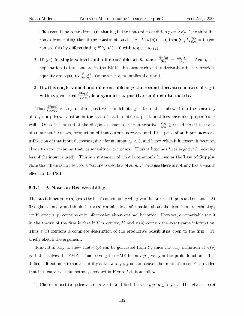
that it is convex. The method, depicted in Figure 5.4, is as follows:
1. Choose a positive price vector p >> 0, and find the set {y|p · y ≤ π (p)}. This gives the set
132
Nolan Miller Notes on Microeconomic Theory: Chapter 5 ver: Aug. 2006
Figure 5.4: Recovering the Technology Set
of points that earn less profit than the optimal production plan, y (p).
2. Since y (p) is the optimal point in Y , we know that Y ⊂ {y|p · y ≤ π (p)}, and that any point
not in {y|p · y ≤ π (p)} cannot be in Y . So, eliminate all points not in {y|p · y ≤ π (p)}. If
output is on the vertical axis and input on the horizontal axis, all points above and to the
right of the price line are eliminated.
3. If we repeat steps 1-2 for all possible positive price vectors, we can eliminate all points that
cannot be in Y for any price vector. And, if Y is convex, every point on the transformation
frontier is optimal for some price vector. Thus by repeating this process we can trace out
the entire transformation frontier, effectively recovering the set Y as
Y = {y|p · y ≤ π (p) for all p >> 0} whenever Y is convex.
The importance of this result is that π (p) is analytically much easier to work with than Y .
But, we should be concerned that by working with π (p) we miss some important features of the
firm’s technology. However, since Y can be recovered in this way, we know that there is no loss of
generality in working with the profit function and net supply functions instead of the full production
set.
5.2 Production with a Single Output
An important special case of production models is where the firm produces a single output using
a number of inputs. In this case, we can make use of a production function (which you probably
133

Nolan Miller Notes on Microeconomic Theory: Chapter 5 ver: Aug. 2006
remember from intermediate micro). In order to distinguish between outputs and inputs, we will
denote the (single) output by q and the inputs by z.5 In contrast to the production-plan approach
examined earlier, inputs will be non-negative vectors when we use this approach, z ∈ RL−1+ . When
there is only one output, the firm’s production set can be characterized by a production function
f (z), where f (z) gives the quantity of output produced when input vector z is employed by the
firm. That is, the relationship between output q and inputs z is given by q = f (z) . The firm’s
production set, Y , can be written as:
Y = {(−z, q) |q − f (z) ≤ 0 and z ≥ 0} .
The analog to the marginal rate of transformation in this model is the marginal rate of
technical substitution. The marginal rate of technical substitution of input j for input i when
output is q is given by:
MRTSji =fj (q)
fi (q).
MRTSji gives the amount by which input j should be decreased in order to keep output constant
following an increase in input i. Note that defined this way, the MRTS between two inputs will be
positive, even though the slope of the production function isoquant is negative.
5.2.1 Profit Maximization with a Single Output
Let p > 0 be the price of the firm’s output and w = (w1, ..., wL−1) ≥ 0 be the prices of the L− 1
inputs, z.6 Thus w · z is the cost of using input vector z. The firm’s profit maximization problem
can be written as
maxz≥0
pq − w · z
s.t : f (z) ≥ q.
Since p > 0, the constraint will always bind. Hence the firm’s problem can be written in terms of
the unconstrained maximization problem:
maxz≥0
pf (z)− w · z.
5For simplicity, we will assume that none of the output will be used to produce the output. For example, electricity
is used to produce electricity. We could easily generalize the model to take account of this possibility.6We should be careful not to confuse w the input price vector with w the consumer’s wealth. This is unfortunate,
but there isn’t much we can do about it.
134
Nolan Miller Notes on Microeconomic Theory: Chapter 5 ver: Aug. 2006
Since this is an unconstrained problem, we don’t need to set up a Lagrangian. However, we do
need to be concerned with “corner solutions” since the firm may not use all inputs in production,
especially if some are very close substitutes. The Kuhn-Tucker first-order conditions are given by:
pfi (z∗)− wi ≤ 0, with equality if z∗i > 0, for ∀ i
As you may recall, fi (z∗) is the marginal product of input zi, the amount by which output increases
if you increase input zi by a small amount. pfi (z∗) is then the amount by which revenue increases
if you increase zi by a small amount, which is sometimes called the marginal revenue product. Of
course, wi is the amount by which cost increases when you increase zi by a small amount. So, the
condition says that at the optimum it must be that the increase in revenue due to increasing zi
by a small amount is less than the increase in cost. If z∗i > 0, then the increase in revenue must
exactly equal the increase in cost. If z∗i = 0, then it may be that pfi (z∗) < wi, meaning that the
increase in revenue due to using even a small amount of input i is not greater than its cost.
We can also rearrange the optimality conditions above to get a familiar tangency condition.
Assume that z∗i and z∗j are strictly positive. Then the above condition can be rewritten as:
fi (z∗)
fj (z∗)=
wi
wj,
which says that the marginal rate of technical substitution between any two inputs must equal the
ratio of their prices. This is just a restatement in this version of the model that the marginal rate
of transformation between any two commodities must equal the ratio of their prices, a condition
we found in the production-plan version of the PMP.
For the case of a single input, this condition becomes pf 0 (z∗) = w, or f 0 (z∗) = wp . Since
inputs are positive, f (z) increases in z on (z1, q) space. Profit isoquant slopes upward at wp , since
pq −wz = k, q = wp z +
kp . Thus, finding f
0 (z∗) = wp means finding the point of tangency between
the profit isoquant and the production function. Graphically, we move the profit line up and to the
left until tangency is found. Note that this is the same thing that is going on in the multiple-input
case: we are finding the tangency between profit and the production function.
We can denote the solution to this problem as z (w, p) , which is called the factor demand
function, since it says how much of the inputs are used at prices p and w. Note that z (w, p) is
an L − 1 dimensional vector. If we plug z (w, p) into the production function, we get q (w, p) =
f (z (w, p)), which is known as the (output) supply function. And, if we plug z (p,w) into the
objective function, we get another version of the firm’s profit function:
135
Nolan Miller Notes on Microeconomic Theory: Chapter 5 ver: Aug. 2006
π (w, p) = pf (z (w, p))−w · z = pq (w, p)− w · z (w, p) .
Note that the firm’s net supply function y (p) that was examined in the previous section is
equivalent to:
y (w, p) = (−z1 (w, p) , ...,−zL−1 (w, p) , q (w, p)) .
Thus you should think of the model we are working with now as a special case of the one from the
previous section, where now we have designated that commodity L is the output and commodities
1 through L− 1 are the inputs, whereas previously we had allowed for any of the commodities to
be either inputs or outputs.
Because of this connection between the single-output model and the production-plan model, the
supply function q (w, p) and factor demand functions z (w, p) will have similar properties to those
enumerated in the previous section. A good test of your understanding would be if you could
reproduce the results regarding the properties of the net supply function y (p) and profit function
π (p) for the single-output model.
5.3 Cost Minimization
Consider the model of profit maximization when there is a single output, as in the previous section.
At price p, let z (w, p) be the firm’s factor demand function and q (w, p) = f (z (w, p)) be the
firm’s supply function. At a particular price vector, (w∗, p∗), let q∗ = q (w∗, p∗) . An interesting
implication of the profit maximization problem is that z∗ = z (w∗, p∗) solves the following problem:
minz
w∗ · z
s.t. : f (z) ≥ q∗.
That is, z∗ is the input bundle that produces q∗ at minimum cost when prices are (w∗, p∗). If a
firm maximizes profit by producing q∗ using z∗, then z∗ is also the input bundle that produces q∗
at minimum cost. The reason for this is clear. Suppose there is another bundle z0 6= z∗ such that
w∗ · z0 < w∗ · z∗ and f (z0) ≥ q∗. But, if this is so, then:
p∗f¡z0¢−w∗ · z0 ≥ p∗q∗ −w∗ · z∗ = p∗f (z∗)− w∗ · z∗,
which contradicts the assumption that z∗ was the profit maximizing input bundle. If there was
another bundle that produced q∗ at lower cost than z∗ does, the firm should have used it in the
136
Nolan Miller Notes on Microeconomic Theory: Chapter 5 ver: Aug. 2006
first place. In other words, a necessary condition for the firm to be profit maximizing is that the
input bundle it chooses minimize the cost of producing that level of output.
The fact that cost minimization is necessary for profit maximization points toward another way
to attack the firm’s problem. First, for any level of output, q, find the input bundle that minimizes
the cost of producing that level of output at the current level of prices. That is, solve the following
problem:
minw · z
s.t. : f (z) ≥ q.
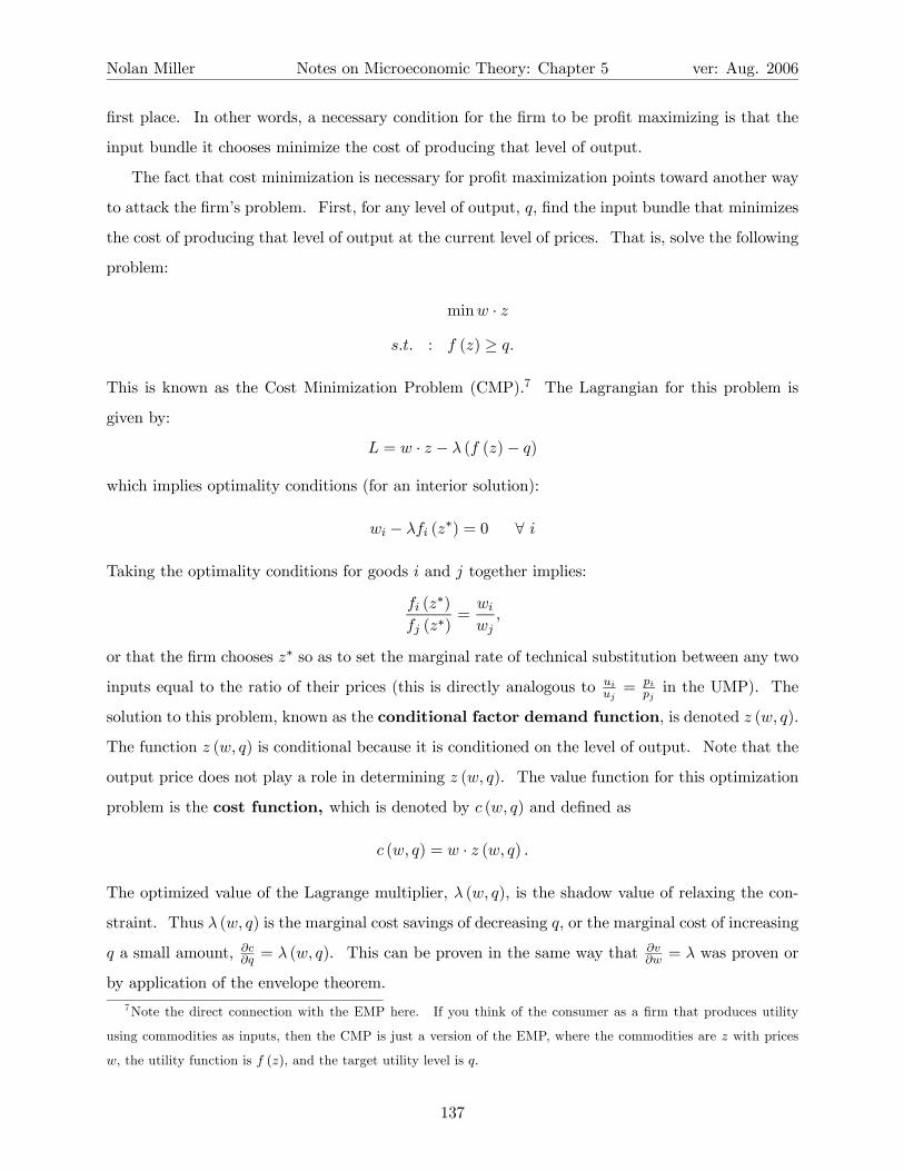
This is known as the Cost Minimization Problem (CMP).7 The Lagrangian for this problem is
given by:
L = w · z − λ (f (z)− q)
which implies optimality conditions (for an interior solution):
wi − λfi (z∗) = 0 ∀ i
Taking the optimality conditions for goods i and j together implies:
fi (z∗)
fj (z∗)=
wi
wj,
or that the firm chooses z∗ so as to set the marginal rate of technical substitution between any two
inputs equal to the ratio of their prices (this is directly analogous to uiuj= pi
pjin the UMP). The
solution to this problem, known as the conditional factor demand function, is denoted z (w, q).
The function z (w, q) is conditional because it is conditioned on the level of output. Note that the
output price does not play a role in determining z (w, q). The value function for this optimization
problem is the cost function, which is denoted by c (w, q) and defined as
c (w, q) = w · z (w, q) .
The optimized value of the Lagrange multiplier, λ (w, q), is the shadow value of relaxing the con-
straint. Thus λ (w, q) is the marginal cost savings of decreasing q, or the marginal cost of increasing
q a small amount, ∂c∂q = λ (w, q). This can be proven in the same way that ∂v
∂w = λ was proven or
by application of the envelope theorem.7Note the direct connection with the EMP here. If you think of the consumer as a firm that produces utility
using commodities as inputs, then the CMP is just a version of the EMP, where the commodities are z with prices
w, the utility function is f (z), and the target utility level is q.
137
Nolan Miller Notes on Microeconomic Theory: Chapter 5 ver: Aug. 2006
The conditional factor demand function gives the least costly way of producing output q when
input prices are w, and the cost function gives the cost of producing that level of output, assuming
that the firm minimizes cost. Thus we can rewrite the firm’s profit maximization problem in terms
of the cost function:
maxq
pq − c (w, q) .
In other words, the firm’s problem is to choose the level of output that maximizes profit, given
that the firm will choose the input bundle that minimizes the cost of producing that level of output
at the current input prices, w. Solving this problem will yield the same input usage and output
production as if the PMP had been solved in its original form.
5.3.1 Properties of the Conditional Factor Demand and Cost Functions
As always, there are a number of properties of the cost function. Once again, they are similar to the
properties derived in the consumer’s version of this problem, the EMP. We start with properties
of z (w, q):
1. z (w, q) is homogeneous of degree zero in w. The usual reason applies. Since the
optimality condition determining z (w, q) is a tangency condition, and the slope of the profit
isoquant and the marginal rate of substitution between any pair of quantities is unaffected
by scaling w to aw, for a > 0, the cost-minimizing point is also unaffected by this scaling
(although the cost of that point will be).
2. If {z ≥ 0|f (z) ≥ q} is convex, then z (w, q) is a convex set. If {z ≥ 0|f (z) ≥ q} is
strictly convex, then z (w, q) is single-valued. Again, the usual argument applies.
Next, there are properties of the cost function c (w, q).
1. c (w, q) is homogeneous of degree one in w. This follows from the fact that z (w, q) is
homogeneous of degree zero in w. c (aw, q) = aw · z (aw, q) = aw · z (w, q) = ac (w, q).
2. c (w, q) is non-decreasing in q. This one is straightforward. Suppose that c (w, q0) >
c (w, q) but q0 < q. In this case, q = f (z (w, q)) > q0, so z (w, q) is feasible in the CMP
for w and q0, and c (w, q) < c (w, q0), which contradicts the assumption that q0 was optimal.
Basically, this property just means that if you want to produce more output, you have to use
more inputs, and as long as inputs are not free, this means that you will incur higher cost.
138
Nolan Miller Notes on Microeconomic Theory: Chapter 5 ver: Aug. 2006
3. c (w, q) is a concave function of w. The argument is exactly the same as the argument
for why the expenditure function is concave. Let wa = aw + (1− a)w0.
c (wa, q) = aw · z (wa, q) + (1− a)w0 · z (wa, q)
≥ aw · z (w, q) + (1− a)w0 · z¡w0, q
¢= ac (w, q) + (1− a) c
¡w0, q
¢.
As usual, going from the first to second line is the crucial step, and the inequality follows
from the fact that z (wa, q) produces output q but is not the cost minimizing way to do so at
either w or w0.
The next properties relate z (w, q) and c (w, q):
1. Shepard’s Lemma. If z (w, q) is single valued at w, then ∂c(w,q)∂wi
= zi (w, q). Again, proof
is by application of the envelope theorem or by using the first-order conditions. I’ll leave this
one as an exercise for you. Hint: Think of c (w, q) as e (p, u), and z (w, q) as h (p, u).
2. If z (w, q) is differentiable, then ∂2c(w,q)∂wi∂wj
=∂zj(w,q)∂wi
= ∂zi(w,q)∂wj
. Again, the proof is the
same.
3. If z (w, q) is differentiable, then the matrix of second derivativesh∂2c(w,q)∂wi∂wj
iis a
symmetric (see number 2 above) negative semi-definite (since c (w, q) is concave)
matrix.
5.3.2 Return to Recoverability
Previously we showed that the profit function contains all of the same information as the firm’s
production set Y . Surprisingly, the firm’s cost function also contains all of the same information
as Y under certain conditions (namely, that the production function is quasiconcave). In order to
show this, we have to show that Y can be recovered from c (w, q), and that c (w, q) can be derived
from Y . Since the cost function is generated by solving the cost minimization problem, c (w, q)
can clearly be derived from Y . Thus all we have to show is that Y can be recovered from c (w, q).
The method is similar to the method used to recover Y from π (p).
Begin by fixing an output quantity, q. Then, choose an input price vector w and find the set
{z ≥ 0|w · z ≥ c (w, q)} .
139
Nolan Miller Notes on Microeconomic Theory: Chapter 5 ver: Aug. 2006
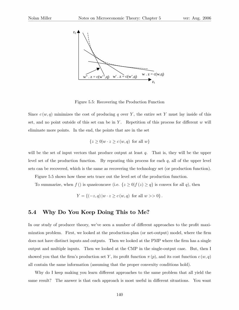
z1
z2
w . z = c(w,q)w' . z = c(w’,q)w'' . z = c(w’’,q)
Figure 5.5: Recovering the Production Function
Since c (w, q) minimizes the cost of producing q over Y , the entire set Y must lay inside of this
set, and no point outside of this set can be in Y . Repetition of this process for different w will
eliminate more points. In the end, the points that are in the set
{z ≥ 0|w · z ≥ c (w, q) for all w}
will be the set of input vectors that produce output at least q. That is, they will be the upper
level set of the production function. By repeating this process for each q, all of the upper level
sets can be recovered, which is the same as recovering the technology set (or production function).
Figure 5.5 shows how these sets trace out the level set of the production function.
To summarize, when f () is quasiconcave (i.e. {z ≥ 0|f (z) ≥ q} is convex for all q), then
Y = {(−z, q) |w · z ≥ c (w, q) for all w >> 0} .
5.4 Why Do You Keep Doing This to Me?
In our study of producer theory, we’ve seen a number of different approaches to the profit maxi-
mization problem. First, we looked at the production-plan (or net-output) model, where the firm
does not have distinct inputs and outputs. Then we looked at the PMP where the firm has a single
output and multiple inputs. Then we looked at the CMP in the single-output case. But, then I
showed you that the firm’s production set Y , its profit function π (p), and its cost function c (w, q)
all contain the same information (assuming that the proper convexity conditions hold).
Why do I keep making you learn different approaches to the same problem that all yield the
same result? The answer is that each approach is most useful in different situations. You want
140
Nolan Miller Notes on Microeconomic Theory: Chapter 5 ver: Aug. 2006
to pick and choose the proper approach, depending on the problem you are working with.
The production-plan approach is useful for proving very general propositions, and necessary to
deal with situations where you don’t know which commodities will be inputs and which will be
outputs. This approach is widely used in the study of general equilibrium, where the output of
one industry is the input of another.
The CMP approach actually turns out to be very useful. We often have better data on the cost
a firm incurs than its production function. But, thanks to the recoverability results, we know that
the cost information contains everything we want to know about the firm. Thus the cost-function
approach can be very useful from an empirical standpoint.
In addition, recall that the PMP is not very useful for technologies with increasing returns to
scale. This is not so with the CMP. The CMP is perfectly well-defined as long as the production
function is quasiconcave, even if it exhibits increasing returns. Hence the CMP may allow us to
say things about firms when the PMP does not.
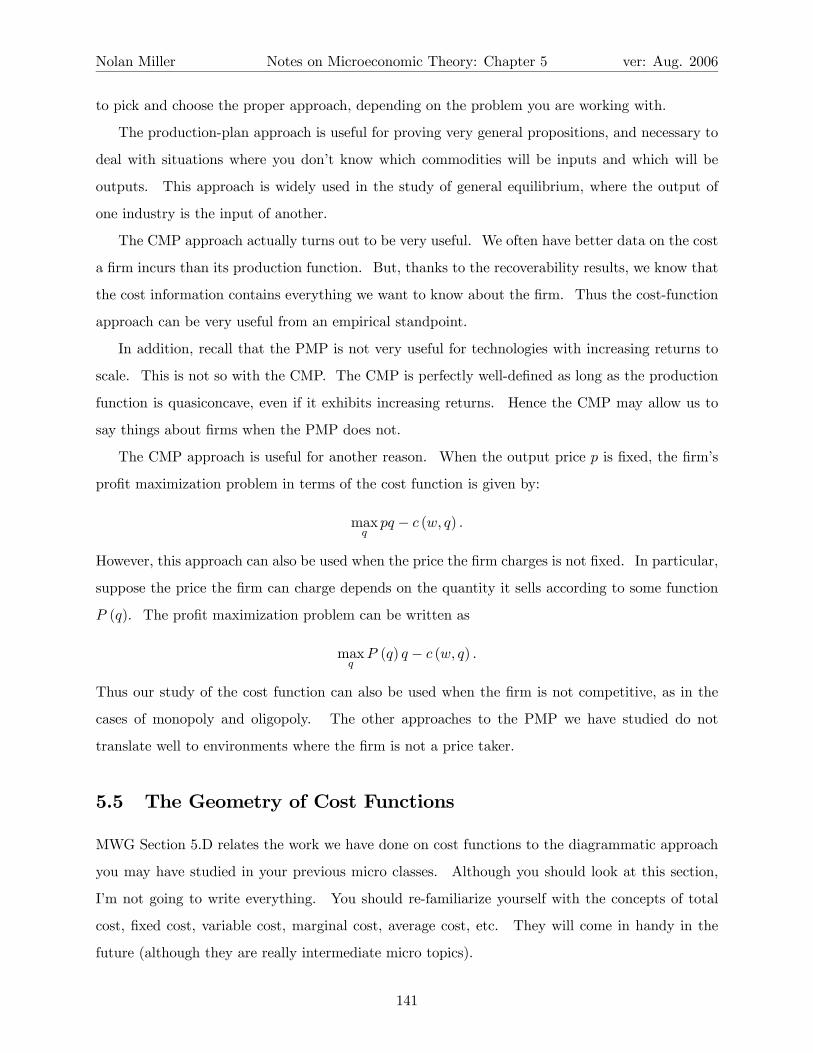
The CMP approach is useful for another reason. When the output price p is fixed, the firm’s
profit maximization problem in terms of the cost function is given by:
maxq
pq − c (w, q) .
However, this approach can also be used when the price the firm charges is not fixed. In particular,
suppose the price the firm can charge depends on the quantity it sells according to some function
P (q). The profit maximization problem can be written as
maxq
P (q) q − c (w, q) .
Thus our study of the cost function can also be used when the firm is not competitive, as in the
cases of monopoly and oligopoly. The other approaches to the PMP we have studied do not
translate well to environments where the firm is not a price taker.
5.5 The Geometry of Cost Functions
MWG Section 5.D relates the work we have done on cost functions to the diagrammatic approach
you may have studied in your previous micro classes. Although you should look at this section,
I’m not going to write everything. You should re-familiarize yourself with the concepts of total
cost, fixed cost, variable cost, marginal cost, average cost, etc. They will come in handy in the
future (although they are really intermediate micro topics).
141
Nolan Miller Notes on Microeconomic Theory: Chapter 5 ver: Aug. 2006
5.6 Aggregation of Supply
MWG summarizes this topic by saying, “If firms maximize profits taking prices as given, then the
production side of the economy aggregates beautifully.” To this let me add that the whole problem
with aggregation on the consumer side was with wealth effects. Since there is no budget constraint
here, there are no wealth effects, and thus there is no problem aggregating.
To aggregate supply, just add up the individual supply functions. Let there be m producers,
and let ym (p) be the net supply function for the mth firm. Aggregate supply can be written as:
yT (p) =MXm=1
ym (p) .
In fact, we can easily think of the aggregate production function as having been produced by
an aggregate producer. Define the aggregate production set Y T = Y 1+ ...+YM , where Y m is the
production set of the mth consumer. Thus Y T represents the opportunities that are available if all
sets are used together. Now, consider yT in Y T . This is an aggregate production plan. It can be
divided into parts, yT1, ..., yTM , where yTm ∈ Y m andP
m yTm = yT . That is, it can be divided
into parts, each of which lies in the production set of some firm. Fix a price vector p∗ and consider
the profit maximizing aggregate supply vector yT (p∗). The question we want to ask is this: Can
yT (p∗) be divided into parts yTm (p∗) such that yTm (p∗) = ym (p∗) andP
m yTm (p∗) = yT (p∗)? In
other words, is it the case that the profit maximizing production plan for the aggregate production
set is the same as would be generated by allowing each of the firms to maximize profit separately
and then adding up the profit-maximizing production plans for each firm? The answer is yes.
For all strictly positive prices, p >> 0, yT (p) =P
ym (p), and πT (p) =P
m πm (p). Thus the
aggregate profit obtained by each firm maximizing profit is the same as is attained by choosing the
profit-maximizing production plan from the aggregate production set.
The fact that production aggregates so nicely is a big help because aggregation tends to convexify
the production set. For example, see MWG 5.E.2. Even if each individual firm’s production
possibilities are non-convex, as in panel a), when you aggregate production possibilities and look
at the average production set, it becomes almost convex. Since non-convexities are a big problem
for economists, it is good to know that when you aggregate supply, the problems tend to go away.
142

Nolan Miller Notes on Microeconomic Theory: Chapter 5 ver: Aug. 2006
5.7 A First Crack at the Welfare Theorems
When economists talk about the fundamental theorems of welfare economics, they are really not
talking about welfare at all. What they are really talking about is efficiency. This is because,
traditionally, economists have not been willing to say what increases society’s “welfare,” since doing
so involves making judgments about how the benefits of various people should be compared. These
kind of judgments, which deal with equity or fairness, it is thought, are not the subject of pure
economics, but of public policy and philosophy.
However, while economists do not like to make equity judgments, we are willing to make the
following statement: Wasteful things are bad. That is, if you are doing something in a wasteful
manner, it would be better if you didn’t. That (unfortunately) is what we mean by welfare.
Actually, I’m giving economists too hard a time. The reason why we focus on wastefulness
(or efficiency) concerns is that while there will never be universal agreement on what is fair, there
can be universal agreement on what is wasteful. And as long as we believe that wastefulness is
bad, then anything that is fair can be made more fair by eliminating its wastefulness, at least in
principle.
Now let’s put this idea in practice. We will consider the question of whether profit maximizing
firms will choose production plans that are not wasteful. We will call a production plan y ∈ Y
efficient if there is no vector y0 ∈ Y such that y0i ≥ yi for all i, and y0 6= y. In other words, a
production plan is efficient if there is no other feasible production plan that could either: 1) produce
the same output using fewer inputs (i.e. y0j = yj and y0k > yk, where j denotes the output goods
and k denotes at least one of the input goods; y0k > yk when y0 uses less of input k, since y0k is
less negative than yk); or 2) produce greater output using the same amount of inputs (i.e. y0j > yj
and y0k = yk, where j denotes at least one of the output goods and k denotes all the input goods).
Thus, production plans that are not efficient are wasteful.
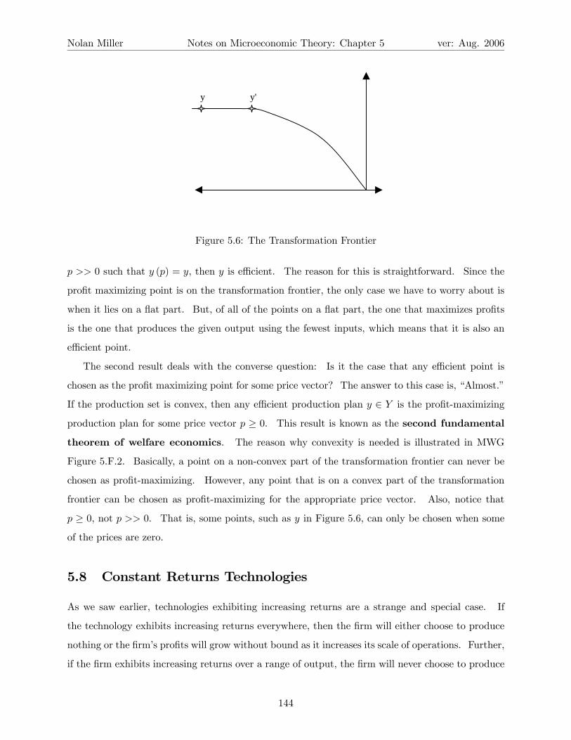
Efficient production plans are located on the firm’s transformation frontier. But, note that
there may be points on the transformation frontier that are not efficient, as is the case in Figure
5.6, where the transformation frontier has a horizontal segment. Points on the interior of the
horizontal part produce the same output as the point furthest to the right on the flat part, but use
more inputs. Hence they are not efficient (i.e., they are wasteful).
The first result, which is a version of the first fundamental theorem of welfare economics,
says that if a production plan is profit maximizing, then it is efficient. Formally, if there exists
143
Nolan Miller Notes on Microeconomic Theory: Chapter 5 ver: Aug. 2006
y y'
Figure 5.6: The Transformation Frontier
p >> 0 such that y (p) = y, then y is efficient. The reason for this is straightforward. Since the
profit maximizing point is on the transformation frontier, the only case we have to worry about is
when it lies on a flat part. But, of all of the points on a flat part, the one that maximizes profits
is the one that produces the given output using the fewest inputs, which means that it is also an
efficient point.
The second result deals with the converse question: Is it the case that any efficient point is
chosen as the profit maximizing point for some price vector? The answer to this case is, “Almost.”
If the production set is convex, then any efficient production plan y ∈ Y is the profit-maximizing
production plan for some price vector p ≥ 0. This result is known as the second fundamental
theorem of welfare economics. The reason why convexity is needed is illustrated in MWG
Figure 5.F.2. Basically, a point on a non-convex part of the transformation frontier can never be
chosen as profit-maximizing. However, any point that is on a convex part of the transformation
frontier can be chosen as profit-maximizing for the appropriate price vector. Also, notice that
p ≥ 0, not p >> 0. That is, some points, such as y in Figure 5.6, can only be chosen when some
of the prices are zero.
5.8 Constant Returns Technologies
As we saw earlier, technologies exhibiting increasing returns are a strange and special case. If
the technology exhibits increasing returns everywhere, then the firm will either choose to produce
nothing or the firm’s profits will grow without bound as it increases its scale of operations. Further,
if the firm exhibits increasing returns over a range of output, the firm will never choose to produce
144
Nolan Miller Notes on Microeconomic Theory: Chapter 5 ver: Aug. 2006
an output on the interior of this range. It will either choose the smallest or largest production plan
on the segment with increasing returns.
Because of the difficulties involved with increasing returns technologies, we tend to focus on
nonincreasing returns technologies. But, nonincreasing returns technologies can be divided into
two groups: technologies that exhibit decreasing returns and technologies that exhibit constant
returns.
In the single-output case, decreasing returns technologies are characterized by strictly concave
production functions. For example, a firm that uses machinery and labor to produce output may
have a production function of the Cobb-Douglas form:
q = f (zm, zl) = bz13mz
13l ,
where b > 0 is some positive real number (for the moment). This production function exhibits
decreasing returns to scale:
f (azm, azl) = b (azm)13 (azl)
13 = a
23 kzmzl = a
23 f (zm, zl) .
We can tell a story accounting for decreasing returns in this case. Suppose the firm has a
factory, and in it are some machines and some workers. At low levels of output, there is plenty
of room for the machines and workers. However, as output increases, additional machines and
workers are hired, and the factory begins to get crowded. Soon, the workers and machines begin
to interfere with each other, making them less productive. Eventually, the place gets so crowded
that nobody can get any work done. This is why the firm experiences decreasing returns to scale.
While the preceding story is realistic, notice that it depends on the fact that the size of the
factory is fixed. To put it another way, if the firm’s plant just kept growing as it hired more
workers and machines, they would never interfere with each other. Because of this, there would
be no decreasing returns.
The point of the argument I just gave is to point out that decreasing returns can usually be
traced back to some fixed input into the productive process that has not been recognized. In
this case, it was the fact that the firm’s factory was fixed. To illustrate, suppose that the b from
the previous production function really had to do with the fixed level of the plant. In particular,
suppose b = (zb)13 , where zb is the current size of the firm’s plant (building). Taking this into
account, the firm’s production function is really:
f (xm, xl, xb) = x13b x
13mx
13l ,
145
Nolan Miller Notes on Microeconomic Theory: Chapter 5 ver: Aug. 2006
and this production function exhibits constant returns to scale.
To paraphrase MWG on this point (bottom of p. 134), the production set Y represents techno-
logical possibilities, not limits on resources. If a firm’s current production plan can be replicated,
i.e., build an identical plant and fill it with identical machines and workers, then it should exhibit
constant returns to scale. Of course, it may not actually be possible to replicate everything in
practice, but it should be possible in theory. Because of this, it has been argued that decreasing
returns must reflect the underlying scarcity of an input into the productive process. Frequently
this is managerial know-how, special locations, or something else. However, if this factor could be
varied, the technology would exhibit constant returns. Because of this, many people believe that
constant returns technologies are the most important sub-category of convex technologies. And,
because of that, we’ll spend a little time looking at some of the peculiar features of constant returns
production functions.
Suppose that the firm produces output q from inputs labor (L) and capital (K) according to
q = f (K,L). If f () exhibits constant returns,
q = f (tK, tL) ≡ tf (K,L) , for any t > 0.
Since this holds for any t, it also holds for t = 1q . Making this substitution:
1 = f
µK
q,L
q
¶.
If we let Kq = k and L
q = l, then we can write the previous statement as:
f (k, l) = 1,
where k is the amount of capital used to produce one unit of output and l is the amount of labor
used to produce one unit of output.
To see why this is important, consider the following cost minimization problem:
minK,L
rK + sL
s.t. f (K,L) = q,
where r is the price of capital and s is the price of labor. We can rewrite this problem as:
minK,L
qrK + sL
q
s.t.1
qf (K,L) = 1,
146

Nolan Miller Notes on Microeconomic Theory: Chapter 5 ver: Aug. 2006
but 1qf (K,L) = f³Kq ,
Lq
´= f (k, l). Thus the CMP becomes:
min q (rk + sl)
s.t. f (k, l) = 1.
Thus if we want to solve the firm’s CMP, we can first find the cost-minimizing way to produce one
unit of output at the current input prices, and then replicate this production plan q times.
In other words, we can learn everything we want to know about the firm’s production function
by studying a single isoquant — in this case the unit isoquant.
As another special case of a constant returns technology, we can think of the situation where
the firm only has a finite number of alternative production plans. For example, suppose that it
can either produce 1 unit of output using 5 units of capital and 3 unit of labor or 2 units of capital
and 7 units of labor. Frequently we will call the different production plans in this environment
“activities.” Thus activity 1 is (5, 3) and activity 2 is (2, 7).
If the firm has the two activities above, then it can produce one unit of output using either
inputs (5, 3) or inputs (2, 7). But, we can also allow the firm to mix the two activities. Thus it
can also produce one unit of output by producing 0 ≤ a ≤ 1 units of output using activity 1 and
1 − a units of output using activity 2. Hence for a firm with these two activities available, the
firm’s unit isoquant consists of the curve:
(k, 3) when k > 5
a (5, 3) + (1− a) (2, 7) for a ∈ [0, 1]
(2, l) for l > 7.
Figure 5.7 depicts this unit isoquant. Note that the vertical and horizontal segments follow from
our assumption of free disposal. Also note that if we had more activities, we would begin to
trace out something that looks like the nicely differentiable isoquants we have been dealing with
all along. Thus differentiable isoquants can be thought of as the limit of having many activities
and the “convexification” process we did above.
As a final point, let me make a connection to something you might have seen in your macro
classes. Go back to:
q = f (tK, tL) ≡ tf (K,L) , for any t > 0.
Instead of dividing by q, as we did above, we can divide by the available labor, L. If we do this,
147

Nolan Miller Notes on Microeconomic Theory: Chapter 5 ver: Aug. 2006
(5,3)
(2,7)
k
L
q = 1
Figure 5.7: The Unit Isoquant
we get:q
L= f
µK
L, 1
¶.
Here we have a version of the production function that gives per capita output as a function of
capital. This is something that is useful in macro models. I just wanted to show you that this
formula, which you may have seen, is grounded in the production theory we have been studying.
5.9 Household Production Models
Now that we have studied both consumer and producer theories, we can begin to think about how
these parts fit together. Chapter 7 explores this topic at the level of the whole economy, but here
we start by looking at the individual household as the unit of both production and consumption.
In particular, we consider consumers who are able to produce one of the commodities using (at
least in part) their own labor. Consider, for example, a consumer who owns a small farm and has
preferences over leisure and consumption of the farm’s output, which we will call “food.” Labor
for the farm can either be provided by the farmer or by hiring labor from the market, and food
produced by the farm can either be consumed internally by the farmer or sold on the market. Thus
it appears that the farmer’s decision about how much leisure and food to consume is intertwined
with his decision about how much food to produce on the farm and how much labor to hire.
However, we will show that if the market for labor is complete, then the farmer’s production and
consumption decisions can be separated. The farmer can maximize utility by first choosing the
amount of total labor that maximizes profit from the farm and then deciding how much of the labor
he will provide himself.
148

Nolan Miller Notes on Microeconomic Theory: Chapter 5 ver: Aug. 2006
5.9.1 Agricultural Household Models with Complete Markets
Models of situations such as we’ve been talking about are known as Agricultural Household Models
(AHM). The version I’ll give you here is a simplification of the model in Bardhan and Udry,
Development Microeconomics, Chapter 2.
Consider a farm owner who can either work on the farm, work off the farm, or not work (leisure).
Similarly, he can use his farm land for his own farming, rent it to others to use, or not use it. In
addition, the farmer can buy additional labor from the market or rent additional land from the
market. Total output produced by the farm depends on the total land used and total labor used
on the farm.
We assume that the farmer faces a complete set of markets and that the buying and selling
prices for food, labor, and land are the same. Let p be the price of output, w be the price of labor
and r be the rental price of land.8
The farmer has utility defined over consumption of food and leisure:
u (c, l)
where c is consumption and l is leisure per person.
The total size of the output is given by
F (L,A)
where L is the total amount of labor employed on the farm and A is the total amount of land that
is cultivated.
The farmer owns a farm with AE acres. These acres can either be used on the farm or rented
to others on the market. Let AU be the number of acres used on the farm and AS be the number
of acres rented to (sold to) others. Since the farmer gets no utility from having idle land, it
is straightforward to show that all acres will either be used internally or rented to the market.
Similarly, the farmer has initial endowment of LE of labor. Let LU and LS be the number of units
of labor that are used on the farm and sold to the market, respectively. Thus we have two resource
constraints:
AE = AU +AS
LE = LU + LS + l.8The natural units are for w to be the price per day of labor and r to be the price per season of an acre of land.
149
Nolan Miller Notes on Microeconomic Theory: Chapter 5 ver: Aug. 2006
These constraints say that all land is either used internally or sold to the market, and all labor
is either used internally, sold to the market, or consumed as leisure.
Let AB and LB, respectively, be the number of units of land and labor bought from the market.
Total labor used on the farm is then given by:
L = LU + LB
and total land used on the farm is given by:
A = AU +AB.
The household’s utility maximization problem can be written as:
maxu (c, l)
s.t :
wLB + rAB ≤ p (F (L,A)− c) + wLS + rAS
L = LU + LB
A = AU +AB
l = LE − LU − LS
0 = AE −AU −AS.
The first constraint is a budget constraint. The left-hand side consists of expenditure on labor
(wLB) and land (rAB) purchased from the market. The right-hand side consists of net revenue
from selling the crop to the market (the price is p, and the amount sold is equal to total production
F (L,A) less the amount consumption internally, c), plus revenue from selling labor to the market
wLS and revenue from selling land to the market rAS. The remaining constraints are the definitions
of land and labor used on the farm and the resource constraints on available time and land.
Through simplification, the constraints can be rewritten as:
w (LB − LS) + r (AB −AS) ≤ p (F (L,A)− c)
L− LU = LB
l − LE + LU = −LS
A−AU = AB
AU −AE = −AS .
150
Nolan Miller Notes on Microeconomic Theory: Chapter 5 ver: Aug. 2006
or
w (L+ l − LE) + r (A−AE) ≤ p (F (L,A)− c)
or
wl + pc ≤ pF (L,A)−wL+wLE − rA+ rAE
or
wl + pc ≤ Π+ wLE + rAE
Π = pF (L,A)− wL− rA.
The last version says that the total expenditure on commodities, wl+ pc, must be less than the
profit earned by running the farm, Π, plus the value of the farmer’s initial endowment, wLE+rAE .
But, notice that L and A appear only on the right-hand side of the budget constraint. Because of
this, we can solve the farmer’s problem in two stages. First, solve
maxL,A
pF (L,A)−wL− rA
for the optimal total labor and land to be used on the farm. Second, solve the farmer’s utility
maximization problem:
maxl,c
u (c, l)
s.t. : wl + pc ≤ Π∗ +wLE + rAE
where
Π∗ = maxL,A
pF (L,A)− wL− rA
is the maximum profit that can be generated on the farm at prices p, w, and r.
What does this mean? Well, the variables l and c have to do with the farmer’s consumption
decisions. The variables L and A have to do with his production decisions. The essence of this
result says that if you want to solve the farmer’s overall utility maximization problem, you can
separate his production and consumption decisions. First, choose the production variables that
maximize the profit produced on the farm.9 Then, choose the consumption bundle that maximizes9There is some degeneracy in the solution to this problem. To see why, suppose the farmer owns 100 acres of
land and chooses to cultivate 80 acres himself. Based on the math of the problem, the farmer is indifferent between
using 80 acres of his own land and renting 20 on the outside market and, for example, renting all 100 acres of his
own land on the market and renting 80 different acres from the market. For simplicity, we’ll just assume that the
farmer first uses his own land and rents any remaining land to the market (or, if A > AE , that he uses all of his own
land and rents the remainder from the market).
151
Nolan Miller Notes on Microeconomic Theory: Chapter 5 ver: Aug. 2006
utility subject to the “ordinary” budget constraint, where wealth is the sum of maximized profit
and endowment wealth. To put it another way, the farmer has two separate decisions to make:
how much land and labor to use on the farm, and how much leisure and food to consume. These
two decisions can be made separately. In particular, the farmer can decide how much labor to use
on the farm without deciding how much of his own labor he should use on the farm. Similarly,
the farmer can decide how much food to produce without deciding how much food he, himself, is
going to consume.
The result stated in the previous paragraph is known as the separation property of the AHP:
When markets are complete, the production and consumption decisions of the household are sep-
arate from each other. The farmer chooses total labor and land in order to maximize profit, and
then chooses how much labor and land to consume as if in an ordinary UMP, where wealth is the
sum of maximized profit from production and endowment wealth.
The separation property is an implication of utility maximization and complete markets, and
it arises endogenously as an implication of the model. Completeness of markets plays a critical
role in the result. For our purposes, a market is complete if the farmer can buy or sell as much of
the commodity as he wants at a particular price that is the same regardless of whether the farmer
buys or sells. A market can fail to be complete if either the price at which someone buys an item
is different than the price at which he sells the item, or if there are limits on the quantity that can
be bought or sold of an item.10
A graphical illustration of the separation property may help. For illustration (because three
dimensional graphs are hard to draw), we will assume that there is no market for land. The farmer
has AE = A∗ acres of land, and uses them all on the farm. The first stage of the optimization
problem is to choose the amount of labor to use on the farm. This is done by maximizing the
profit earned on the farm, pc − wL, subject to the constraint that c = F (L,A∗). This profit
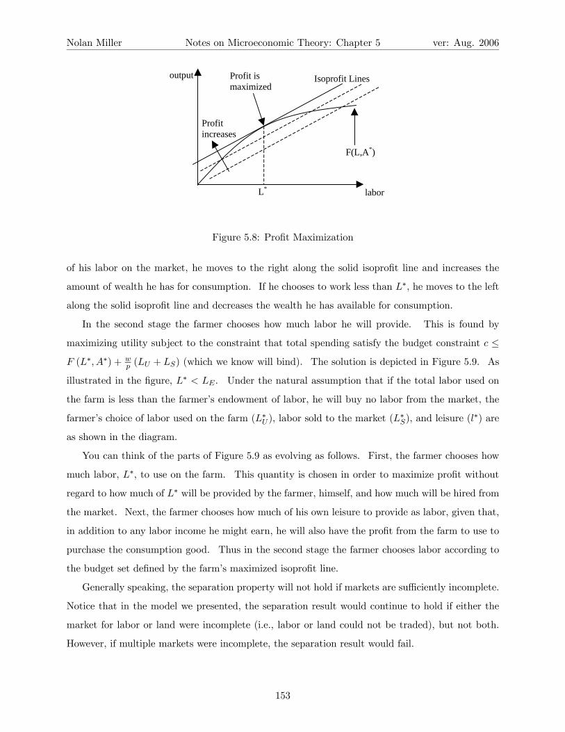
maximization problem is illustrated in Figure 5.8. Thus the first stage in the farmer’s decision
results in L∗ units of labor being used on the farm. When this amount of labor is used, the farm’s
profit is given by the level of the solid black isoprofit line at L∗. The equation of this line is given
by c = F (L∗, A∗) + wp (LU + LS).11 If the farmer chooses to work more than L∗ by selling some
10One of the chief “market failures” in developing economies is incompleteness of labor markets. It is often
impossible to buy labor regardless of the price offered because it is costly for the people who have jobs to find the
people who are willing to work.11This isoprofit line makes intuitive sense if you think about it as a budget line. Consumption equals the total
product of the farm plus the value of labor provided by the farmer, normalized to the units of consumption (w/p).
152
Nolan Miller Notes on Microeconomic Theory: Chapter 5 ver: Aug. 2006
Isoprofit Lines
Profitincreases
Profit ismaximized
F(L,A*)
L* labor
output
Figure 5.8: Profit Maximization
of his labor on the market, he moves to the right along the solid isoprofit line and increases the
amount of wealth he has for consumption. If he chooses to work less than L∗, he moves to the left
along the solid isoprofit line and decreases the wealth he has available for consumption.
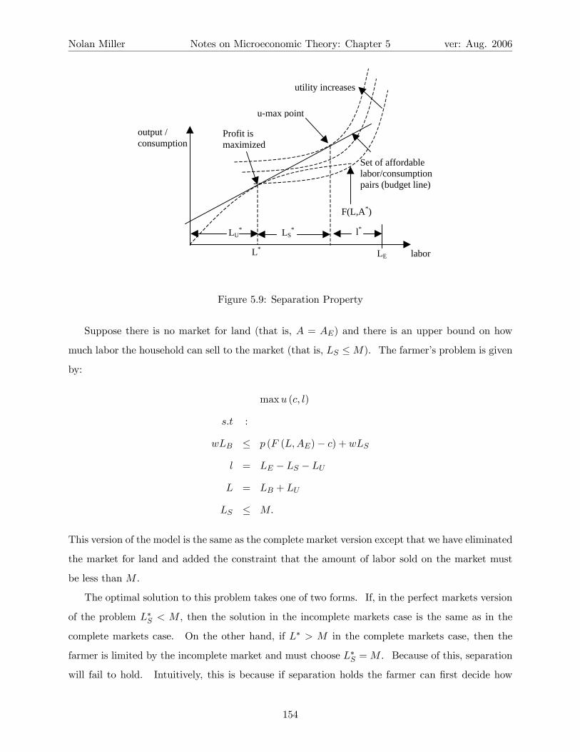
In the second stage the farmer chooses how much labor he will provide. This is found by
maximizing utility subject to the constraint that total spending satisfy the budget constraint c ≤
F (L∗, A∗) + wp (LU + LS) (which we know will bind). The solution is depicted in Figure 5.9. As
illustrated in the figure, L∗ < LE. Under the natural assumption that if the total labor used on
the farm is less than the farmer’s endowment of labor, he will buy no labor from the market, the
farmer’s choice of labor used on the farm (L∗U ), labor sold to the market (L∗S), and leisure (l
∗) are
as shown in the diagram.
You can think of the parts of Figure 5.9 as evolving as follows. First, the farmer chooses how
much labor, L∗, to use on the farm. This quantity is chosen in order to maximize profit without
regard to how much of L∗ will be provided by the farmer, himself, and how much will be hired from
the market. Next, the farmer chooses how much of his own leisure to provide as labor, given that,
in addition to any labor income he might earn, he will also have the profit from the farm to use to
purchase the consumption good. Thus in the second stage the farmer chooses labor according to
the budget set defined by the farm’s maximized isoprofit line.
Generally speaking, the separation property will not hold if markets are sufficiently incomplete.
Notice that in the model we presented, the separation result would continue to hold if either the
market for labor or land were incomplete (i.e., labor or land could not be traded), but not both.
However, if multiple markets were incomplete, the separation result would fail.
153
Nolan Miller Notes on Microeconomic Theory: Chapter 5 ver: Aug. 2006
Profit ismaximized
F(L,A*)
L* labor
output /consumption
Set of affordablelabor/consumptionpairs (budget line)
utility increases
LE
u-max point
LU* l*LS
*
Figure 5.9: Separation Property
Suppose there is no market for land (that is, A = AE) and there is an upper bound on how
much labor the household can sell to the market (that is, LS ≤M). The farmer’s problem is given
by:
maxu (c, l)
s.t :
wLB ≤ p (F (L,AE)− c) + wLS
l = LE − LS − LU
L = LB + LU
LS ≤ M.
This version of the model is the same as the complete market version except that we have eliminated
the market for land and added the constraint that the amount of labor sold on the market must
be less than M .
The optimal solution to this problem takes one of two forms. If, in the perfect markets version
of the problem L∗S < M , then the solution in the incomplete markets case is the same as in the
complete markets case. On the other hand, if L∗ > M in the complete markets case, then the
farmer is limited by the incomplete market and must choose L∗S =M . Because of this, separation
will fail to hold. Intuitively, this is because if separation holds the farmer can first decide how
154
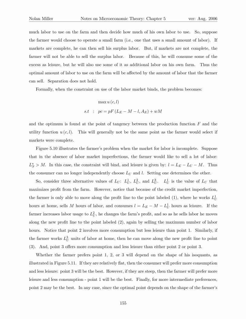
Nolan Miller Notes on Microeconomic Theory: Chapter 5 ver: Aug. 2006
much labor to use on the farm and then decide how much of his own labor to use. So, suppose
the farmer would choose to operate a small farm (i.e., one that uses a small amount of labor). If
markets are complete, he can then sell his surplus labor. But, if markets are not complete, the
farmer will not be able to sell the surplus labor. Because of this, he will consume some of the
excess as leisure, but he will also use some of it as additional labor on his own farm. Thus the
optimal amount of labor to use on the farm will be affected by the amount of labor that the farmer
can sell. Separation does not hold.
Formally, when the constraint on use of the labor market binds, the problem becomes:
maxu (c, l)
s.t : pc = pF (LE −M − l, AE) +wM
and the optimum is found at the point of tangency between the production function F and the
utility function u (c, l). This will generally not be the same point as the farmer would select if
markets were complete.
Figure 5.10 illustrates the farmer’s problem when the market for labor is incomplete. Suppose
that in the absence of labor market imperfections, the farmer would like to sell a lot of labor:
L∗S > M. In this case, the constraint will bind, and leisure is given by: l = LE − LU −M . Thus
the consumer can no longer independently choose LU and l. Setting one determines the other.
So, consider three alternative values of LU : L1U , L2U , and L3U . L1U is the value of LU that
maximizes profit from the farm. However, notice that because of the credit market imperfection,
the farmer is only able to move along the profit line to the point labeled (1), where he works L1U
hours at home, sells M hours of labor, and consumes l = LE −M − L1U hours as leisure. If the
farmer increases labor usage to L2U , he changes the farm’s profit, and so as he sells labor he moves
along the new profit line to the point labeled (2), again by selling the maximum number of labor
hours. Notice that point 2 involves more consumption but less leisure than point 1. Similarly, if
the farmer works L3U units of labor at home, then he can move along the new profit line to point
(3). And, point 3 offers more consumption and less leisure than either point 2 or point 3.
Whether the farmer prefers point 1, 2, or 3 will depend on the shape of his isoquants, as
illustrated in Figure 5.11. If they are relatively flat, then the consumer will prefer more consumption
and less leisure: point 3 will be the best. However, if they are steep, then the farmer will prefer more
leisure and less consumption - point 1 will be the best. Finally, for more intermediate preferences,
point 2 may be the best. In any case, since the optimal point depends on the shape of the farmer’s
155
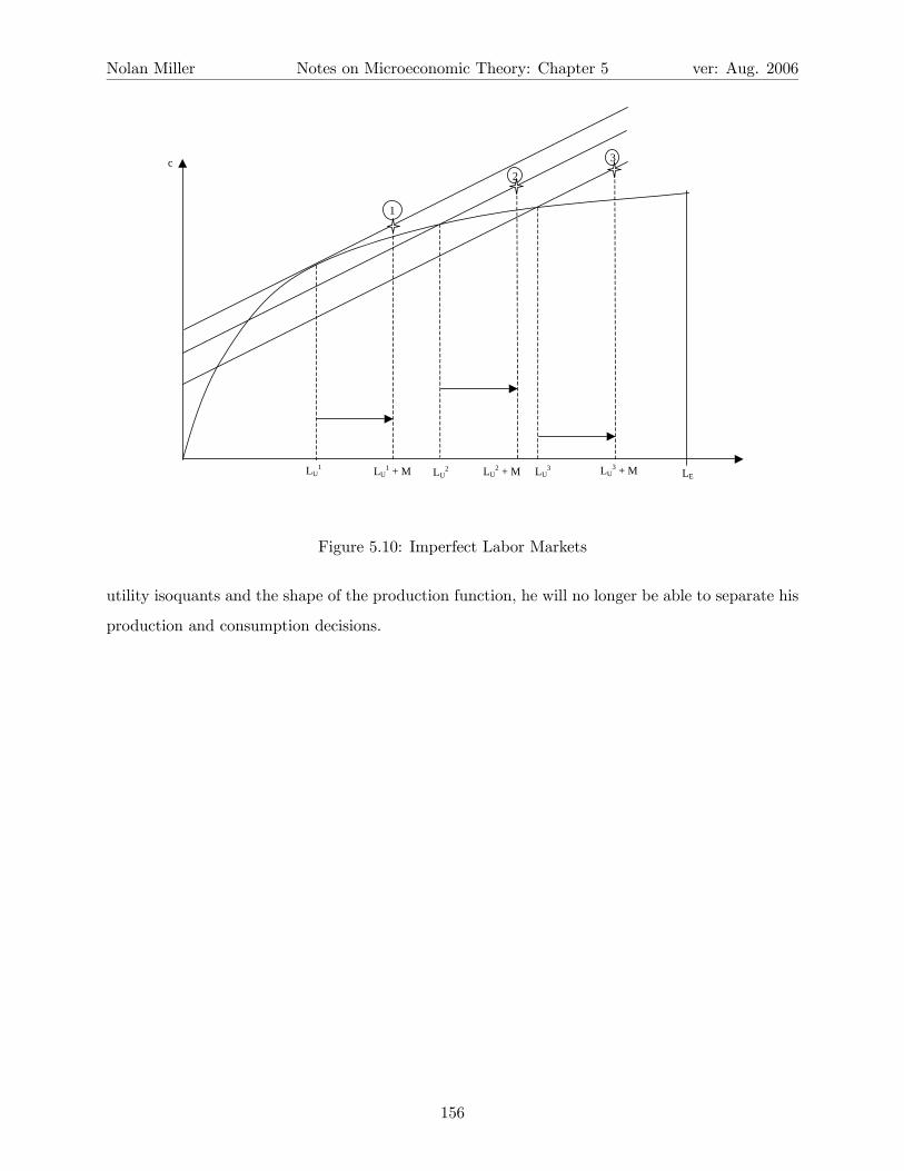
Nolan Miller Notes on Microeconomic Theory: Chapter 5 ver: Aug. 2006
LU1 + M LU
2 + M LU3 + MLU
1 LU2 LU
3
1
2
3c
LE
Figure 5.10: Imperfect Labor Markets
utility isoquants and the shape of the production function, he will no longer be able to separate his
production and consumption decisions.
156

Nolan Miller Notes on Microeconomic Theory: Chapter 5 ver: Aug. 2006
LU1 + M LU
2 + M LU3 + MLU
1 LU2 LU
3
1
2
3c
LE
Figure 5.11: AHP Without Separation
157