Processing XML Streams with Deterministic Automata and ...suciu/paper-tods2004.pdf · Processing...
48
Processing XML Streams with Deterministic Automata and Stream Indexes Todd J. Green University of Pennsylvania Ashish Gupta University of Washington Gerome Miklau University of Washington Makoto Onizuka NTT Cyber Space Laboratories, NTT Corporation and Dan Suciu University of Washington 1. INTRODUCTION Several applications of XML stream processing have emerged recently: content- based XML routing [Snoeren et al. 2001], selective dissemination of information (SDI) [Altinel and Franklin 2000; Chan et al. 2002; Diao et al. 2003], continuous queries [Chen et al. 2000], and processing of scientific data stored in large XML files [Higgins et al. 1992; Thierry-Mieg and Durbin 1992; Borne ]. They commonly need to process a large collection of XPath expressions (say 10,000 to 1,000,000), on a continuous stream of XML data, at a high sustained throughput. For illustration, consider XML Routing [Snoeren et al. 2001]. Here a network of XML routers forwards a continuous stream of XML packets from data producers to consumers. A router forwards each XML packet it receives to a subset of its output links (other routers or clients). Forwarding decisions are made by evaluating a large number of XPath filters, corresponding to clients’ subscription queries, on the stream of XML packets. Data processing is minimal: there is no need for the router to have an internal representation of the packet, or to buffer the packet after it has forwarded it. Performance, however, is critical, and [Snoeren et al. 2001] reports very poor performance with publicly available XPath processing tools. Our goal is to develop techniques for evaluating a large collection of XPath expres- sions on a stream of XML packets. First we describe a technique that guarantees a sustained throughput, which is largely independent of the number of XPath expres- sions. In contrast, in all other techniques proposed for processing XPath expressions the throughput decreases as the number of XPath expressions increases. [Altinel and Franklin 2000; Chan et al. 2002; Diao et al. 2003]. Second, we describe a lightweight binary data structure, called Stream IndeX (SIX), which can be added to the XML packets for further speedups. The first and main contribution is to show that a Deterministic Finite Automaton ACM Transactions on Computational Logic, Vol. ??, No. 4, 12 2004, Pages 1–0??.
Transcript of Processing XML Streams with Deterministic Automata and ...suciu/paper-tods2004.pdf · Processing...
Processing XML Streams with DeterministicAutomata and Stream Indexes
Todd J. Green
University of Pennsylvania
Ashish Gupta
University of Washington
Gerome Miklau
University of Washington
Makoto Onizuka
NTT Cyber Space Laboratories, NTT Corporation
and
Dan Suciu
University of Washington
1. INTRODUCTION
Several applications of XML stream processing have emerged recently: content-based XML routing [Snoeren et al. 2001], selective dissemination of information(SDI) [Altinel and Franklin 2000; Chan et al. 2002; Diao et al. 2003], continuousqueries [Chen et al. 2000], and processing of scientific data stored in large XMLfiles [Higgins et al. 1992; Thierry-Mieg and Durbin 1992; Borne ]. They commonlyneed to process a large collection of XPath expressions (say 10,000 to 1,000,000),on a continuous stream of XML data, at a high sustained throughput.
For illustration, consider XML Routing [Snoeren et al. 2001]. Here a network ofXML routers forwards a continuous stream of XML packets from data producers toconsumers. A router forwards each XML packet it receives to a subset of its outputlinks (other routers or clients). Forwarding decisions are made by evaluating alarge number of XPath filters, corresponding to clients’ subscription queries, on thestream of XML packets. Data processing is minimal: there is no need for the routerto have an internal representation of the packet, or to buffer the packet after it hasforwarded it. Performance, however, is critical, and [Snoeren et al. 2001] reportsvery poor performance with publicly available XPath processing tools.
Our goal is to develop techniques for evaluating a large collection of XPath expres-sions on a stream of XML packets. First we describe a technique that guarantees asustained throughput, which is largely independent of the number of XPath expres-sions. In contrast, in all other techniques proposed for processing XPath expressionsthe throughput decreases as the number of XPath expressions increases. [Altineland Franklin 2000; Chan et al. 2002; Diao et al. 2003]. Second, we describe alightweight binary data structure, called Stream IndeX (SIX), which can be addedto the XML packets for further speedups.
The first and main contribution is to show that a Deterministic Finite AutomatonACM Transactions on Computational Logic, Vol. ??, No. 4, 12 2004, Pages 1–0??.
2 · Todd J. Green et al.
(DFA) can be used effectively to process a large collection of XPath expressions,at guaranteed throughput. Our approach is to convert all XPath expressions intoa single DFA, then evaluate it on the input XML stream. DFAs are the mostefficient means to process XPath expressions, but they were thought to be uselessfor workloads with a large number of XPath expressions, because their size growsexponentially with size of the workload.
Our solution to the state explosion problem consists of constructing the DFAlazily. A lazy DFA is one whose states and transitions are computed from thecorresponding NFA at runtime, not at compile time. A new entry in the transitiontable or a new state is computed only when the input data requires the DFA tofollow that transition or enter that state. The transitions and states in the lazyDFA form a subset of those in the standard DFA, which we call eager DFA in thispaper. As a consequence, the lazy DFA can sometimes be much smaller than theeager DFA.
We show that, for XML processing, the number of states in the lazy DFA is smalland depends only on the structure of the XML data. It is largely independent onthe number of XPath expressions in the workload. More precisely, the size ofthe lazy DFA is at most the size of the data guide [Goldman and Widom 1997]of the XML data, which is typically very small for XML data that has a fairlyregular structure. In hindsight, after we first announced this result in [Green et al.2003], this fact may sound obvious, but it was far from obvious before. Previouswork in this area [Altinel and Franklin 2000; Chan et al. 2002; Diao et al. 2003]explicitly avoided using DFAs, and developed alternative processing techniques thatare slower, but have guaranteed space bounds.
To support the claim that the number of states in the lazy DFA is small, wepresent here a series of theoretical results characterizing the size of both the eagerand the lazy DFA for XPath expressions. These results are of general interest inXPath processing, beyond stream applications.
The second contribution in this paper consists of a light-weight technique forspeeding up processing XML documents in a network application. The observationhere is that, in many applications processing streams of XML messages, the mainbottleneck consists of parsing, or tokenizing each message. To address that, somecompanies use a proprietary tokenized format instead of the XML text representa-tion [Florescu et al. 2003], but this suffers from lack of interoperability. We proposea more lightweight technique, that adds a small amount of binary data to eachXML document, facilitating access into the document. We call this data a StreamIndeX (SIX). The SIX is computed once, when the XML document is first gener-ated, and attached somehow to the document (for example using DIME [Corp. ]).All applications receiving the document that understand the SIX can then accessthe XML data much faster. If they don’t understand the SIX, then they can fallback on the traditional parse/evaluate model. Space-wise, the overhead of a SIXis very small (typical values are, say, 7% of the data, and can be reduced further),so there is little or no penalty from using it. We note that the general principleof adding a small amount of binary data to facilitate access in the XML documentalso admits other implementations, see [Gupta et al. 2002; Gupta et al. 2003].
Finally, we illustrate an application of our techniques by describing the XMLACM Transactions on Computational Logic, Vol. ??, No. 4, 12 2004.
Processing XML Streams with Deterministic Automata and Stream Indexes · 3
Toolkit (XMLTK), for highly scalable processing of XML files. Our goal is toprovide to the public domain a collection of stand-alone XML tools, in analogywith Unix commands for text files. Current tools include sorting, aggregation,nesting, unnesting, and a converter from a directory hierarchy to an XML file. Eachtool performs one single kind of transformation, but can scale to arbitrarily largeXML documents in, essentially, linear time, and using only a moderate amount ofmain memory. By combining tools in complex pipelines users can perform complexcomputations on the XML files. There is a need for such tools in user communitiesthat have traditionally processed data formatted in line-oriented text files, such asnetwork traffic logs, web server logs, telephone call records, and biological data.Today, many of these applications are done by combinations of Unix commands,such as grep, sed, sort, and awk. All these data formats can and should betranslated into XML, but then all the line-oriented Unix commands become useless.Our goal is to provide tools that can process the data after it has been migrated toXML.
Discussion This paper focuses only on linear XPath expressions. Applicationsrarely have such simple workloads, and are more likely to use XPath expressionswith nested predicates. Scalable techniques for such workloads require a separateinvestigation and are out of the scope of this paper. However, the techniques de-scribed here are relevant to the general XPath processing problem, for two reasons.First, processing linear expressions is a subproblem in processing more complexworkloads, and needs to be addressed somehow. In fact we describe here a simpleway to evaluate XPath expressions with nested predicates by decomposing theminto linear fragments, and we found this simple technique to work well on smallworkloads. Second, at a deeper level, it has been shown in [Gupta and Suciu 2003]that our results about the DFA extend, although not in a trivial way, to a pushdownautomaton, which can process an arbitrarily complex workload of XPath expres-sions with nested predicates. Thus, the results and techniques discussed in thispaper can be seen as building blocks for more powerful processors.
Paper Organization We begin with an overview in Sec. 2 of the processingmodel and the system’s architecture. We describe in detail processing with a DFAin Sec. 3, then discuss its construction in Sec. 4 and analyze its size. We describethe SIX in Sec. 5. We report our experimental results in Sec. 6 and describe theXML Toolkit in Sec. 7. Sec 8 contains related work, and we conclude in Sec. 9.The Appendix contains some of the proofs and more details on the XML Toolkit.
2. OVERVIEW
2.1 The Event-Based Processing Model
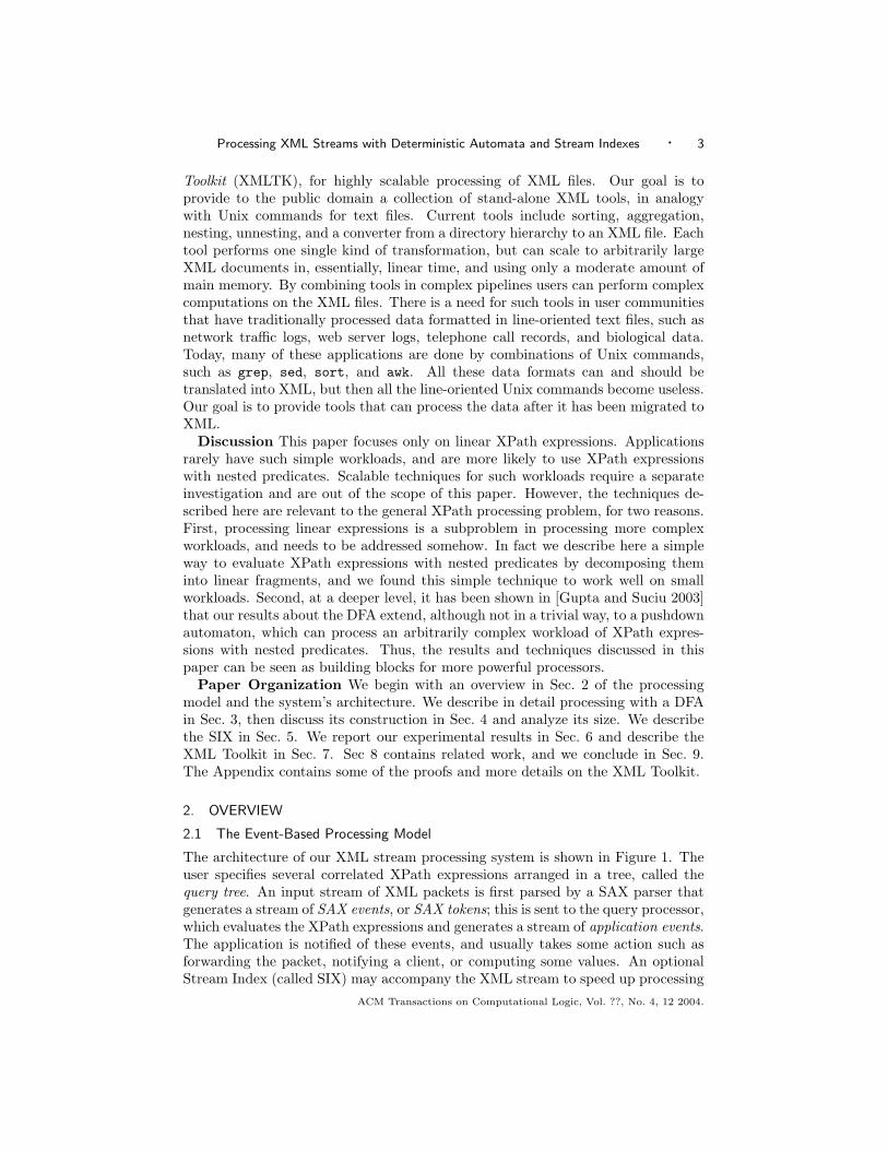
The architecture of our XML stream processing system is shown in Figure 1. Theuser specifies several correlated XPath expressions arranged in a tree, called thequery tree. An input stream of XML packets is first parsed by a SAX parser thatgenerates a stream of SAX events, or SAX tokens; this is sent to the query processor,which evaluates the XPath expressions and generates a stream of application events.The application is notified of these events, and usually takes some action such asforwarding the packet, notifying a client, or computing some values. An optionalStream Index (called SIX) may accompany the XML stream to speed up processing
ACM Transactions on Computational Logic, Vol. ??, No. 4, 12 2004.
4 · Todd J. Green et al.
SIX Manager
SAX Parser Application
XML
Stream
SIX
Stream
Tree Pattern
skip(k)
skip(k)
SAX Events Application Events
(Lazy DFA)
Query Processor
Fig. 1. System’s Architecture
(Section 5).We consider linear XPath expressions, P , given by the following grammar:
P ::= /N | //N | PP
N ::= E | A | ∗ | text() | text() = S (1)
Here E and A are element label and attribute label respectively, / denotes thechild axis, // denotes the descendant axis, ∗ is the wild card, and S is a stringconstant. As explained earlier, nested predicates are not discussed here, and haveto be decomposed into linear XPath expressions, as shown below.
A query tree, Q, has nodes labeled with variables and the edges with linear pathexpressions. There is a distinguished variable, $R, which is always bound to theroot node of the XML packet. Each node in the tree also carries a boolean flag,called sax f. When its value is true, then the SAX events under that node areforwarded to the application; otherwise they are not forwarded to the application.The sax f can be set on and off at various nodes in the query tree. The sax f flagis used by the stream index, Sec. 5.
Example 2.1 The following is a query tree (tags taken from the NASA dataset [Borne]):
$D IN $R/datasets/dataset$H IN $D/history$T IN $D/title sax f = true$TH IN $D/tableHead sax f = true$N IN $D//tableHead//*$F IN $TH/field$V IN $N/text()="Galaxy"
Fig. 2 shows this query tree graphically. Here the application requests the SAXevents under $T, and $TH only. Fig. 3 shows the result of evaluating this querytree on an XML input stream: the first column shows the XML stream, the secondshows the SAX events generated by the parser, and the last column shows theevents forwarded to the application. Only some of the SAX events are seen by theapplication, namely exactly those that occur within a $T or $TH variable event.
Nested Predicates When an XPath expression contains nested predicates, thenthe application needs to decompose them into linear XPath expressions. For exam-ACM Transactions on Computational Logic, Vol. ??, No. 4, 12 2004.

Processing XML Streams with Deterministic Automata and Stream Indexes · 5
/datasets/dataset
/history /tableHead/title
$F
$D
$T $N $H $TH
$V
$R
/field
//tableHead//*
/text("Galaxy")sax_f=true
sax_f=true
Fig. 2. A Query Tree
XML Stream Parser Events: Application Events:SAX Events SAX and variable events
<datasets> startElement(datasets) startVariable($R)<dataset> startElement(dataset) startVariable($D)<history> startElement(history) startVariable($H)<date> startElement(date)10/10/59 text("10/10/59")</date> endElement(date)</history> endElement(history) endVariable($H)<title> startElement(title) startVariable($T)
startElement(title)<subtitle> startElement(subtitle) startElement(subtitle)Study text("Study") text("Study")</subtitle> endElement(subtitle) endElement(subtitle)</title> endElement(title) endElement(title)
endVariable($T)</dataset> endElement(dataset) endVariable($D)</datasets> endElement(datasets) endVariable($R)
Fig. 3. Events generated by a Query Tree
ACM Transactions on Computational Logic, Vol. ??, No. 4, 12 2004.
6 · Todd J. Green et al.
Q: Q’:
$Y IN $R/catalog/product $Y IN $R/catalog/product
$Z IN $Y/@category/text()="tools" $Z IN $R/catalog/product/@category/text()="tools"
$U IN $Y/sales/@price $U IN $R/catalog/product/sales/@price
$X IN $Y/quantity $X IN $R/catalog/product/quantity
Fig. 4. A query tree Q and an equivalent query set Q′ of absolute XPath expressions.
ple, given the expression:
$X IN $R/catalog/product[@category="tools"][sales/@price > 200]/quantity
the application needs to decompose it into four linear XPath expression, which formthe query tree Q shown in Fig. 4. The query processor will notify the application offive events, $R, $Y, $Z, $U, $X, and the application needs to do extra work to combinethese events, as follows. It uses two boolean variables, b1, b2. On a $Z event, itsets b1 to true; on a $U event test the following text value and, if it is > 200,then sets b2 to true. At the end of a $Y event it checks whether b1=b2=true.Some extra care is needed for the descendant axis, //. This simple method workswell in the case when there are few XPath expressions, like in the XML Toolkitdescribed in Sec. 7. Workloads with large numbers of XPath expressions and nestedpredicates require more complex processing techniques, and this is outside of thescope of this paper. We note, however, that the DFA-based processing method thatwe study in this paper has been incorporated into a highly scalable technique forXPath expressions with nested predicates [Gupta and Suciu 2003].
The Event-based Processing Problem The problem that we address is: givena query tree Q, pre-process it, and then evaluate it on an incoming XML stream.The goal is to maximize the throughput at which we can process the XML stream.
The special case that we will study in Section 4 is that of a query tree in whichevery XPath expression is absolute, i.e. starts at the root node. In that case wecall Q a query set, or simply a set, because it just consists of a set of absoluteXPath expressions. For the purpose of application events only, a query tree Q canbe rewritten into an equivalent query set Q′, as illustrated in Fig. 4. Moreoverthe DFAs for Q and Q′ are isomorphic, so it suffices to study the size of the DFAonly for absolute path expressions (Sec. 4). However, in practice the DFA for Qis somewhat more efficient to compute than that for Q′, and for that reason thequery processor works on the query tree Q directly.
3. PROCESSING WITH DFAS
3.1 Generating a DFA from a Query Tree
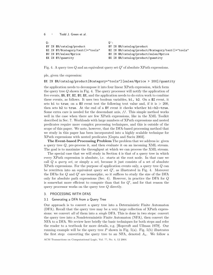
Our approach is to convert a query tree into a Deterministic Finite Automaton(DFA). Recall that the query tree may be a very large collection of XPath expres-sions: we convert all of them into a single DFA. This is done in two steps: convertthe query tree into a Nondeterministic Finite Automaton (NFA), then convert theNFA to a DFA. We review here briefly the basic techniques for both steps and referthe reader to a textbook for more details, e.g. [Hopcroft and Ullman 1979]. Ourrunning example will be the query tree P shown in Fig. 5(a). Fig. 5(b) illustratesthe first step: converting the query tree to an NFA, denoted An. We follow aACM Transactions on Computational Logic, Vol. ??, No. 4, 12 2004.

Processing XML Streams with Deterministic Automata and Stream Indexes · 7
popular method for converting XPath expression into an NFA, which was used inTukwila [Ives et al. 2002], our own work [Green et al. 2003], and in YFilter [Diaoet al. 2003]; for a detailed overview of various methods for converting a regularexpression to an NFA we refer to Watson’s survey [Watson 1993]. In Fig. 5(b), thetransitions labeled ∗ correspond to ∗ or // in P ; there is one initial state; there is oneterminal state for each variable ($X, $Y, . . . ); and there are ε-transitions. The latterare needed to separate the loops from the previous state. For example if we mergestates 2, 3, and 6 into a single state then the ∗ loop (corresponding to //) wouldincorrectly apply to the right branch. This justifies 2 ε→ 3; the other ε-transitionsare introduced by compositional rules, which are straightforward and omitted. No-tice that, in general, the number of states in the NFA, An, is proportional to thesize of P .
Let Σ denote the set of all tags, attributes, and text constants occurring in thequery tree P , plus a special symbol ω representing any other symbol that couldbe matched by ∗ or //. For w ∈ Σ∗ let An(w) denote the set of states in An
reachable on input w. In our example we have Σ = {a, b, d, ω}, and An(ε) = {1},An(ab) = {3, 4, 7}, An(aω) = {3, 4}, An(b) = ∅.
The DFA for P , Ad, has the following set of states and the following transitions:
states(Ad) = {An(w) | w ∈ Σ∗} (2)δ(An(w), a) = An(wa), a ∈ Σ
Our running example Ad is illustrated1 in Fig. 5 (c). Each state has unique tran-sitions, and one optional [other] transition, denoting any symbol in Σ except theexplicit transitions at that state: this is different from ∗ in An which denotes anysymbol. For example [other] at state {3, 4, 8, 9} denotes either a or ω, while[other] at state {2, 3, 6} denotes a, d, or ω. Terminal states may be labeled nowwith more than one variable, e.g. {3, 4, 5, 8, 9} is labeled $Y and $Z. A sax f flagis defined for each DFA state as follows: it value is true if at least one of the NFAstates in that DFA state has sax f = true; otherwise it is false.
3.2 The DFA at Run time
One can process an XML stream with a DFA very efficiently. It suffices to maintaina pointer to the current DFA state, and a stack of DFA states. SAX events areprocessed as follows. On a startElement(e) event we push the current state on thestack, and replace the state with the state reached by following the e transition2;on an endElement(e) we pop a state from the stack and set it as the currentstate. Attributes and text values are handled similarly. At any moment, the statesstored in the stack are exactly those at which the ancestors of the current nodewere processed, and at which one may need to come back later when exploringsubsequent children nodes of those ancestors. If the current state has any variablesassociated to it, then for each such variable $V we send a startVariable($V) (inthe case of a startElement) or endVariable($V) (in the case of a endElement)
1Technically, the state ∅ is also part of the DFA, and behaves like a “failure” state, collecting allmissing transitions. We do not illustrate it in our examples.2The state’s transitions are stored in a hash table.
ACM Transactions on Computational Logic, Vol. ??, No. 4, 12 2004.

8 · Todd J. Green et al.
$X IN $R/a
$Y IN $X//*/b
$Z IN $X/b/*
$U IN $Z/d
$R
/a
//*/b /b/*
/d
$Y $Z
$U
$X
(a)
εε
* b
$Z
*
ε
d
$U
$Y
b
3
6
7
4 8
95
10
*
a
$R
$X
1
2
(b)
a
$R
$X2,3,6
3,4,73,4
[other]
3,4,5
b
b[other] [other]
3,4,5,8,9
b
$Y, $Z
3,4,8,9
$Z
3,4,10
d
$U
[other]
[other]
$Yb
d
[other]
b
b
b
1
[other]
(c)
Fig. 5. (a) A query tree P ; (b) its NFA, An, and (c) its DFA, Ad.
ACM Transactions on Computational Logic, Vol. ??, No. 4, 12 2004.
Processing XML Streams with Deterministic Automata and Stream Indexes · 9
(a)
b
a
b
a
a
*
5
0
1
2
4
3
$X
[other]0
01
012 02
0123 023 013 03
01234 0234 0134 034 . . . .
. . . .
a
a
a
a
a
[other]
[other] [other]
[other] [other]
a
012345
a a a
01345 01245
. . . .
. . . . . . . . .
$X $X $X $X
$X
a
*
*
*
*
*0
5
1
2
4
3
b
a
b
a
a
0[other]
$X
01
02
013
014
025
[other]
[other]
b
[other]
[other] a
[other]
a
(b) (c) (d)
a
0145
a
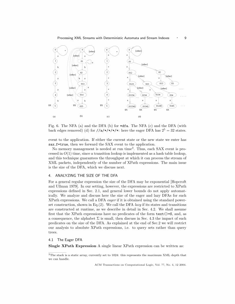
Fig. 6. The NFA (a) and the DFA (b) for *dfa. The NFA (c) and the DFA (withback edges removed) (d) for //a/*/*/*/*: here the eager DFA has 25 = 32 states.
event to the application. If either the current state or the new state we enter hassax f=true, then we forward the SAX event to the application.
No memory management is needed at run time3. Thus, each SAX event is pro-cessed in O(1) time, since a transition lookup is implemented as a hash table lookup,and this technique guarantees the throughput at which it can process the stream ofXML packets, independently of the number of XPath expressions. The main issueis the size of the DFA, which we discuss next.
4. ANALYZING THE SIZE OF THE DFA
For a general regular expression the size of the DFA may be exponential [Hopcroftand Ullman 1979]. In our setting, however, the expressions are restricted to XPathexpressions defined in Sec. 2.1, and general lower bounds do not apply automat-ically. We analyze and discuss here the size of the eager and lazy DFAs for suchXPath expressions. We call a DFA eager if it is obtained using the standard power-set construction, shown in Eq.(2). We call the DFA lazy if its states and transitionsare constructed at runtime, as we describe in detail in Sec. 4.2. We shall assumefirst that the XPath expressions have no predicates of the form text()=S, and, asa consequence, the alphabet Σ is small, then discuss in Sec. 4.3 the impact of suchpredicates on the size of the DFA. As explained at the end of Sec.2 we will restrictour analysis to absolute XPath expressions, i.e. to query sets rather than querytrees.
4.1 The Eager DFA
Single XPath Expression A single linear XPath expression can be written as:
3The stack is a static array, currently set to 1024: this represents the maximum XML depth that
we can handle.
ACM Transactions on Computational Logic, Vol. ??, No. 4, 12 2004.
10 · Todd J. Green et al.
P = p0//p1// . . . //pk
where each pi is N1/N2/ . . . /Nni, i = 0, . . . , k, and each Nj is given by Eq.(1) in
Sec. 2.1. We consider the following parameters:
k = number of //’sni = length of pi, i = 0, . . . , km = max # of ∗’s in each pi
n = length (or depth) of P , i.e.∑
i=0,k ni
s = alphabet size =| Σ |
For example if P = //a/∗//a/∗/b/a/∗/a/b, then k = 2 (p0 = ε, p1 = a/∗, p2 =a/∗/b/a/∗/a/b), s = 3 (Σ = {a, b, ω}), n = 9 (node tests: a, ∗, a, ∗, b, a, ∗, a, b), andm = 2 (we have 2 ∗’s in p2). The following theorem gives an upper bound on thenumber of states in the DFA. The proof is in the Appendix.
Theorem 4.1. Given a linear XPath expression P , define prefix(P ) = n0 andbody(P ) = (k2−1
2k2 (n − n0)2 + 2(n − n0) − nk + 1)sm when k > 0, and body(P ) = 1when k = 0. Then the eager DFA for P has at most prefix(P ) + body(P ) states. Inparticular, if m = 0 and k ≤ 1, then the DFA has at most (n + 1) states.
We first illustrate the theorem in the case where there are no wild-cards (m = 0)and k = 1. Then n = n0 +n1 and there are at most n0 +2(n−n0)−n1 +1 = n+1states in the DFA. For example, if p = //a/b/a/a/b, then k = 1, n = 5: the NFAand DFA are shown in Fig. 6 (a) and (b) respectively, and indeed the latter has 6states. This generalizes to //N1/N2/ . . . /Nn: the DFA has only n + 1 states, andis an isomorphic copy of the NFA plus some back transitions: this corresponds toKnuth-Morris-Pratt’s string matching algorithm [Cormen et al. 1990].
When there are wild cards (m > 0), the theorem gives an exponential upperbound because of the factor sm. There is a corresponding exponential lower bound,illustrated in Fig. 6 (c), (d), showing that the DFA for p = //a/∗/∗/∗/∗, has 25
states. It is easy to generalize this example and see that the DFA for //a/∗/ . . . /∗has 2m+1 states, where m is the number of ∗’s. While a simple hack enables us to//a/∗/ . . . /∗ on an XML document using constant space without converting it intoa DFA, this is no longer possible if we modify the expression to //a/∗/ . . . /∗/b.
Thus, the theorem shows that the only thing that can lead to an exponen-tial growth of the DFA is the maximum number of ∗’s between any two con-secutive //’s. One expects this number to be small in most practical applica-tions; arguably users write expressions like /catalog//product//color ratherthan /catalog//product/*/*/*/*/*/*/*/*/*/color. Some implementations ofXQuery already translate a single linear XPath expression into DFAs [Ives et al.2002].
Multiple XPath Expressions For sets of XPath expressions, the DFA alsogrows exponentially with the number of expressions containing //. We illustratethis first, then state the lower and upper bounds.
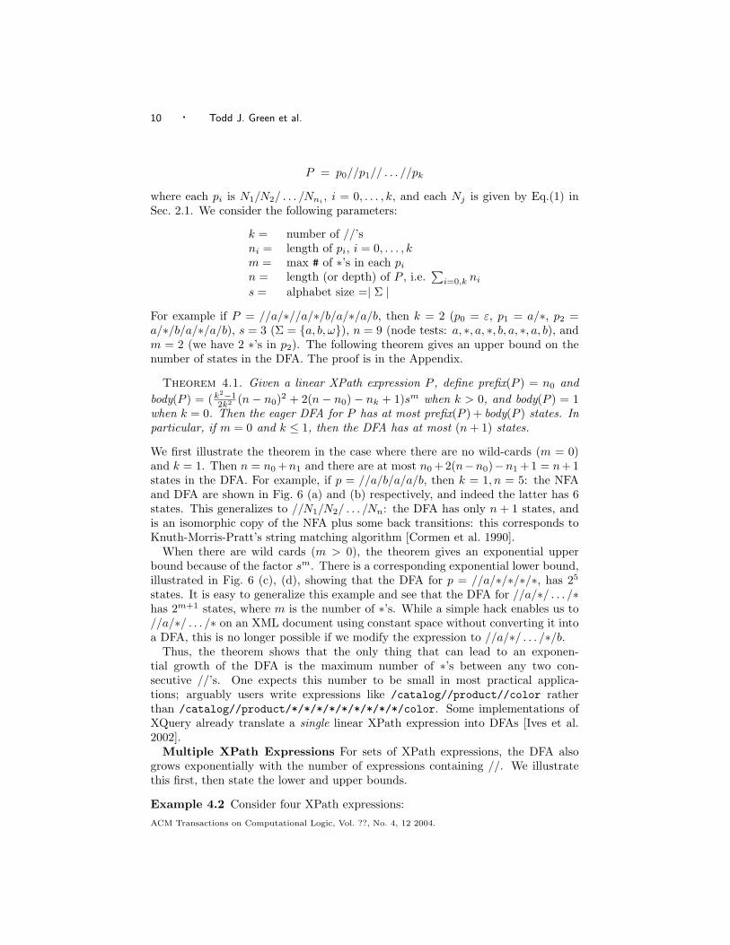
Example 4.2 Consider four XPath expressions:ACM Transactions on Computational Logic, Vol. ??, No. 4, 12 2004.
Processing XML Streams with Deterministic Automata and Stream Indexes · 11
$X1 IN $R//book//figure$X2 IN $R//table//figure$X3 IN $R//chapter//figure$X4 IN $R//note//figure
The eager DFA needs to remember what subset of tags of {book, table, chapter, note}it has seen, resulting in at least 24 states. We generalize this below.
Proposition 4.3. Consider p XPath expressions:$X1 IN $R//a1//b
...$Xp IN $R//ap//b
where a1, . . . , ap, b are distinct tags. Then the DFA has at least 2p states.4
For all practical purposes, this means that the size of the DFA for a set of XPathexpressions is exponential. The theorem below refines the exponential upper bound,and its proof is in the Appendix.
Theorem 4.4. Let Q be a set of XPath expressions. Then the number of statesin the eager DFA for Q is at most:
∑P∈Q(prefix(P )) +
∏P∈Q(1 + body(P )). In
particular, if A,B are constants s.t. ∀P ∈ Q, prefix(P ) ≤ A and body(P ) ≤ B,then the number of states in the eager DFA is ≤ p · A + (1 + B)p′ , where p is thenumber of XPath expressions in Q and p′ is the number of such expressions thatcontain //.
Recall that body(P ) already contains an exponent, which we argued is small inpractice. The theorem shows that the extra exponent added by having multipleXPath expressions is precisely the number of expressions with //’s. This resultshould be compared with Aho and Corasick’s dictionary matching problem [Ahoand Corasick 1975; Rozenberg and Salomaa 1997]. There we are given a dictionaryconsisting of p words, {w1, . . . , wp}, and have to compute the DFA for the set Q ={//w1, . . . , //wp}. Hence, this is a special case where each XPath expression has asingle, leading //, and has no ∗. The main result in the dictionary matching problemis that the number of DFA states is linear in the total size of Q. Theorem 4.4 isweaker in this special case, since it counts each expression with a // toward theexponent. The theorem could be strengthened to include in the exponent onlyXPath expressions with at least two //’s, thus technically generalizing Aho andCorasick’s result. However, XPath expressions with two or more occurrences of// must be added to the exponent, as Proposition 4.3 shows. We chose not tostrengthen Theorem 4.4 since it would complicate both the statement and proof,with little practical significance.
Sets of XPath expressions like the ones we saw in Example 4.2 are common inpractice, and rule out the eager DFA, except in trivial cases. The solution is toconstruct the DFA lazily, which we discuss next.
4Although this requires p distinct tags, the result can be shown with only 2 distinct tags, and
XPath expressions of depths n = O(log p), using binary encoding of tags.
ACM Transactions on Computational Logic, Vol. ??, No. 4, 12 2004.
12 · Todd J. Green et al.
4.2 The Lazy DFA
The lazy DFA is constructed at run-time, on demand. Initially it has a single state(the initial state), and whenever we attempt to make a transition into a missingstate we compute it, and update the transition. The hope is that only a small setof the DFA states needs to be computed.
This idea has been used before in text processing [Laurikari 2000], but it hasnever been applied to large numbers of expressions as required in our applications.A careful analysis of the size of the lazy DFA is needed to justify its feasibility. Weprove two results, giving upper bounds on the number of states in the lazy DFA,that are specific to XML data, and that exploit either the schema, or the dataguide. We stress, however, that neither the schema nor the data guide need to beknown to the query processor in order to use the lazy DFA, and only serve for thetheoretical results.
Formally, let Al be the lazy DFA. Its states and transitions are described by thefollowing equations, which should be compared to Eq.(2) in Sec. 3.1:
states(Al) = {An(w) | w ∈ Ldata} (3)δ(An(w), a) = An(wa), wa ∈ Ldata (4)
Here Ldata is the set of all root-to-leaf sequences of tags in the input XML streams.Thus, the size of the lazy DFA is determined by two factors: (1) the number ofstates, i.e. | states(Al) |, and (2) the size of each state, i.e. | An(w) |, for w ∈ Ldata.Recall that each state in the lazy DFA is represented by a set of states from theNFA, which we call an NFA table. In the eager DFA the NFA tables can be droppedafter the DFA has been computed, but in the lazy DFA they need to be kept, sincewe never really complete the construction of the DFA (they are technically neededto apply Equation (4) at runtime). Therefore the NFA tables also contribute to thesize of the lazy DFA. We analyze in this section both factors.
4.2.1 The number of states in the lazy DFA. The first size factor, the numberof states in the lazy DFA may be, in theory, exponentially large, and hence is ourfirst concern. Assuming that the XML stream conforms to a schema (or DTD),denote Lschema all root-to-leaf sequences allowed by the schema: we have Ldata ⊆Lschema ⊆ Σ∗.
We use graph schema [Abiteboul et al. 1999; Buneman et al. 1997] to formalizeour notion of schema, where nodes are labeled with tags and edges denote inclusionrelationships. A graph schema S is a graph with a designated root node, and withnodes labeled with symbols from Σ. Each path from the root defines a word w ∈ Σ∗,and the set of all such words forms a regular language denoted Lschema. Definea simple cycle, c, in a graph schema to be a set of nodes c = {x0, x1, . . . , xn−1}which can be ordered s.t. for every i = 0, . . . , n − 1, there exists an edge from xi
to x(i+1) mod n. We say that a graph schema is simple, if for any two simple cyclesc 6= c′, we have c ∩ c′ = ∅.
We illustrate with the DTD in Fig. 7, which also shows its graph schema. ThisDTD is simple, because the only cycles in its graph schema (shown in Fig. 7 (a)) areself-loops. All non-recursive DTDs are simple. Recall that a simple path in a graphis a path where each node occurs at most once. For a simple graph schema we denoteACM Transactions on Computational Logic, Vol. ??, No. 4, 12 2004.
Processing XML Streams with Deterministic Automata and Stream Indexes · 13
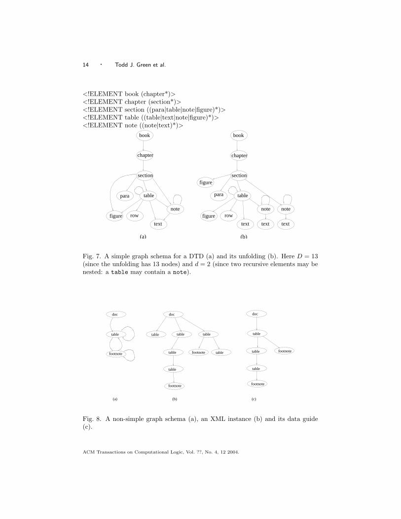
d the maximum number of simple cycles that a simple path can intersect (henced = 0 for non-recursive schemes), and D the total number of nonempty, simple pathsstarting at the root: D can be thought of as the number of nodes in the unfolding5.In our example d = 2, D = 13, since the path book/chapter/section/table/noteintersects two simple cycles, {table} and {note}, and there are 13 different simplepaths that start at the root: they correspond to the nodes in the unfolded graphschema shown in Fig. 7 (b). For a query set Q, denote n its depth, i.e. the maximumnumber of symbols in any P ∈ Q (i.e. the maximum n, as in Sec. 4.1). We provethe following result in the Appendix:
Theorem 4.5. Consider a simple graph schema with d, D, defined as above, andlet Q be a set of XPath expressions of maximum depth n. Then, on any XML inputsatisfying the schema, the lazy DFA has at most 1 + D × (1 + n)d states.
The result is surprising, because the number of states does not depend on thenumber of XPath expressions, only on their depths. In Example 4.2 the depth isn = 2: for the DTD above, the theorem guarantees at most 1 + 13 × 32 = 118states in the lazy DFA. In practice, the depth is larger: for n = 10, the theoremguarantees ≤ 1574 states, even if the number of XPath expressions increases to,say, 100,000. By contrast, the eager DFA may have ≥ 2100000 states (see Prop. 4.3).Fig. 6 (d) shows another example: of the 25 states in the eager DFA only 9 areexpanded in the lazy DFA.
Theorem 4.5 has many applications. First for non-recursive DTDs (d = 0) thelazy DFA has at most 1 + D states6. Second, in data-oriented XML instances,recursion is often restricted to hierarchies, e.g. departments within departments,parts within parts. Hence, their DTD is simple, and d is usually small. Finally, thetheorem also covers applications that handle documents from multiple DTDs (e.g.in XML routing): here D is the sum over all DTDs, while d is the maximum overall DTDs.
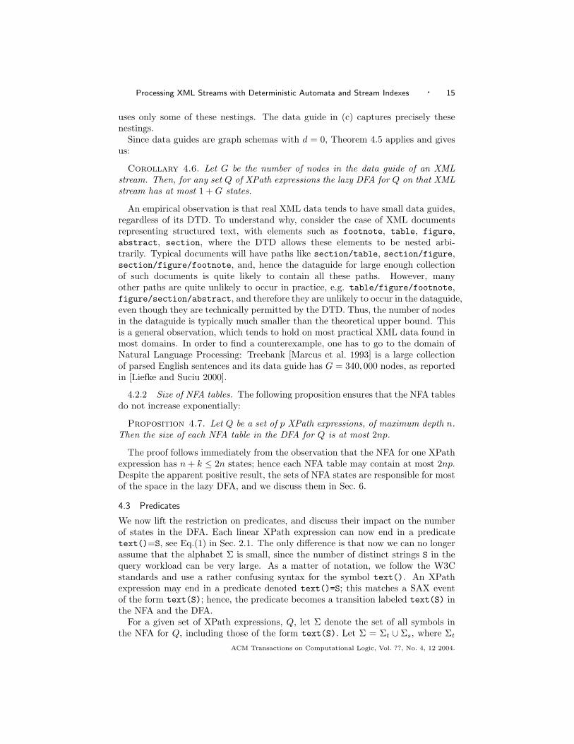
The theorem does not apply, however, to document-oriented XML data. Thesehave non-simple DTDs : for example a table may contain a table or a footnote,and a footnote may also contain a table or a footnote. Hence, both {table}and {table, footnote} are cycles, and they share a node. This is illustrated inFig. 8 (a). For such cases we give an upper bound on the size of the lazy DFA interms of data guides [Goldman and Widom 1997]. Given an XML data instance,the data guide G is that schema which is (a) deterministic7 (b) it captures exactlythe sequence of labels in the data, Lschema = Ldata, and (c) G is unfolded, i.e. it isa tree. The latter property is possible to enforce since Ldata is finite, hence the dataguide has no cycles. Figure 8 illustrates the connection between graph schemas,XML data, and data guides. The graph schema in (a) is non-simple, and showsall possible nestings that are allowed in the data. An actual XML instance in (b)
5The constant D may, in theory, be exponential in the size of the schema because of the unfolding,but in practice the shared tags typically occur at the bottom of the DTD structure (see [Sahuguet2000]), hence D is only modestly larger than the number of tags in the DTD.6This also follows directly from (3) since in this case Lschema is finite and has 1 + D elements:one for w = ε, and one for each non-empty, simple path.7For each label a ∈ Σ, a node can have at most one child labeled with a.
ACM Transactions on Computational Logic, Vol. ??, No. 4, 12 2004.
14 · Todd J. Green et al.
<!ELEMENT book (chapter*)><!ELEMENT chapter (section*)><!ELEMENT section ((para|table|note|figure)*)><!ELEMENT table ((table|text|note|figure)*)><!ELEMENT note ((note|text)*)>
table
note
tablepara
text text text
note note
text
chapter
book
section
chapter
book
rowfigure rowfigure
figuresection
para
(a) (b)
Fig. 7. A simple graph schema for a DTD (a) and its unfolding (b). Here D = 13(since the unfolding has 13 nodes) and d = 2 (since two recursive elements may benested: a table may contain a note).
footnote
(c)(b)(a)
doc
table
footnote
doc
table table table
table footnote
table
table
table
doc
table
table
footnote
footnote
Fig. 8. A non-simple graph schema (a), an XML instance (b) and its data guide(c).
ACM Transactions on Computational Logic, Vol. ??, No. 4, 12 2004.
Processing XML Streams with Deterministic Automata and Stream Indexes · 15
uses only some of these nestings. The data guide in (c) captures precisely thesenestings.
Since data guides are graph schemas with d = 0, Theorem 4.5 applies and givesus:
Corollary 4.6. Let G be the number of nodes in the data guide of an XMLstream. Then, for any set Q of XPath expressions the lazy DFA for Q on that XMLstream has at most 1 + G states.
An empirical observation is that real XML data tends to have small data guides,regardless of its DTD. To understand why, consider the case of XML documentsrepresenting structured text, with elements such as footnote, table, figure,abstract, section, where the DTD allows these elements to be nested arbi-trarily. Typical documents will have paths like section/table, section/figure,section/figure/footnote, and, hence the dataguide for large enough collectionof such documents is quite likely to contain all these paths. However, manyother paths are quite unlikely to occur in practice, e.g. table/figure/footnote,figure/section/abstract, and therefore they are unlikely to occur in the dataguide,even though they are technically permitted by the DTD. Thus, the number of nodesin the dataguide is typically much smaller than the theoretical upper bound. Thisis a general observation, which tends to hold on most practical XML data found inmost domains. In order to find a counterexample, one has to go to the domain ofNatural Language Processing: Treebank [Marcus et al. 1993] is a large collectionof parsed English sentences and its data guide has G = 340, 000 nodes, as reportedin [Liefke and Suciu 2000].
4.2.2 Size of NFA tables. The following proposition ensures that the NFA tablesdo not increase exponentially:
Proposition 4.7. Let Q be a set of p XPath expressions, of maximum depth n.Then the size of each NFA table in the DFA for Q is at most 2np.
The proof follows immediately from the observation that the NFA for one XPathexpression has n + k ≤ 2n states; hence each NFA table may contain at most 2np.Despite the apparent positive result, the sets of NFA states are responsible for mostof the space in the lazy DFA, and we discuss them in Sec. 6.
4.3 Predicates
We now lift the restriction on predicates, and discuss their impact on the numberof states in the DFA. Each linear XPath expression can now end in a predicatetext()=S, see Eq.(1) in Sec. 2.1. The only difference is that now we can no longerassume that the alphabet Σ is small, since the number of distinct strings S in thequery workload can be very large. As a matter of notation, we follow the W3Cstandards and use a rather confusing syntax for the symbol text(). An XPathexpression may end in a predicate denoted text()=S; this matches a SAX eventof the form text(S); hence, the predicate becomes a transition labeled text(S) inthe NFA and the DFA.
For a given set of XPath expressions, Q, let Σ denote the set of all symbols inthe NFA for Q, including those of the form text(S). Let Σ = Σt ∪ Σs, where Σt
ACM Transactions on Computational Logic, Vol. ??, No. 4, 12 2004.
16 · Todd J. Green et al.
contains all element and attribute labels and ω, while Σs contains all symbols ofthe form text(S). The NFA for Q has a special, 2-tier structure: first an NFAover Σt, followed by some Σs-transitions into sink states, i.e. with no outgoingtransitions. The corresponding DFA also has a two-tier structure: first the DFAfor the Σt part, denote it At, followed by Σs transitions into sink states. Allour previous upper bounds on the size of the lazy DFA apply to At. We nowhave to count the additional sink states reached by text(S) transitions. For that,let Σs = {text(S1), . . . , text(Sq)}, and let Qi, i = 1, . . . , q, be the set of XPathexpressions in Q that end in text() = Si; we assume w.l.o.g. that every XPathexpression in Q ends in some predicate in Σs, hence Q = Q1 ∪ . . . ∪ Qq. DenoteAi the DFA for Qi, and At
i its Σt-part. Let si be the number of states in Ati,
i = 1, . . . , q. All the previous upper bounds, in Theorem 4.1, Theorem 4.5, andCorollary 4.6 apply to each si. We prove the following in the Appendix.
Theorem 4.8. Given a set of XPath expressions Q, containing q distinct pred-icates of the form text()=S, the additional number of sink states in the lazy DFAdue to the constant values is at most
∑i=1,q si.
5. THE STREAM INDEX (SIX)
Parsing and tokenizing the XML document is generally accepted to be a major bot-tleneck in XML processing. An obvious solution is to represent an XML documentin binary, as a string of binary tokens. In an XML message system, the messagesare now binary representations of XML, rather than real XML, or they are con-verted into binary when they enter the system. Some commercial implementationsadopt this approach in order to increase performance [Florescu et al. 2003]. Thedisadvantage is that all servers in the network must understand that binary for-mat. This defeats the purpose of the XML standard, which is supposed to addressprecisely the lack of interoperability that is associated with a binary format.
We favor an alternative approach: keep the XML packets in their native textformat, and add a small amount of binary data that allows fast access to thedocument. We describe here one such technique: a different technique based on thesame philosophy is described in [Gupta et al. 2003].
5.1 Definition
Given an XML document, a Stream IndeX (SIX) for that document is an orderedset of byte offsets pairs:
(beginOffset, endOffset)
where beginOffset is the byte offset of some begin tag, and endOffset of thecorresponding end tag (relative to the begin tag). Both numbers are representedin binary, to keep the SIX small. The SIX is computed only once, by the producerof the XML stream, attached to the XML packet somehow (e.g. using the DIMEstandard [Corp. ]), then sent along with the XML stream and used by everyconsumer of that stream (e.g. by every router, in XML routing). A server thatdoes not understand the SIX can simply ignore it.
The SIX is sorted by beginOffset. The query processor starts parsing the XMLdocument and matches SIX entries with XML tags. Depending on the queriesACM Transactions on Computational Logic, Vol. ??, No. 4, 12 2004.

Processing XML Streams with Deterministic Automata and Stream Indexes · 17
that need to be evaluated, the query processor may decide to skip over elementsin the XML document, using endOffset. Thus, a simple addition of two integersreplaces parsing an entire subelement, generating all SAX events, and looking forthe matching end tag. This is a significant savings.
The SIX module (see Fig. 1 in Sec. 2.1) offers a single interface: skip(k), wherek ≥ 0 denotes the number of open XML elements that need to be skipped. Thusskip(0) means “skip to the end of the most recently opened XML element”. Theexample below illustrates the effect of a skip(0) call, issued after reading <c>:
XML stream:<a> <b> <c> <d> </d> </c> <e> </e> </b> <f> . . .
|skip(0)
parser:<a> <b> <c> <e> </e> </b> <f> . . .
while the following shows the effect of a skip(1) call:
XML stream:<a> <b> <c> <d> </d> </c> <e> </e> </b> <f> . . .
|skip(1)
parser:<a> <b> <c> <f> . . .
5.2 Using the SIX
A SIX can be used by any application that processes XML documents using a SAXparser.
Example 5.1 Consider a very simple application counting how many products ina stream of messages have more than 10 complaints:
count(/message/product[count(complaint) >= 10])
While looking for product, if some other tag is encountered then the applicationissues a skip(0). Inside a product, the application listens for complaint: if someother tag is read, then issue a skip(0). If a complaint is read then increment thecount. If the count is >=10 then issue skip(1), otherwise skip(0).
A DFA can use a SIX effectively. From the transition table of a DFA state it cansee what transitions it expects. If a begin tag does not correspond to any transitionand its sax f flag is set to false, then it issues a skip(0). As we show in Sec. 6this results in dramatic speed-ups.
5.3 Implementation
The SIX is very robust: arbitrary entries may be removed without compromisingconsistency. Entries for very short elements are candidates for removal because theyprovide little benefit. Very large elements may need to be removed (as we explainnext), and skipping over them can be achieved by skipping over their children,yielding largely the same benefit.
ACM Transactions on Computational Logic, Vol. ??, No. 4, 12 2004.
18 · Todd J. Green et al.
The SIX works on arbitrarily large XML documents. After exceeding 232 bytesin the input stream, beginOffset wraps around; the only constraint is that eachwindow of 232-bytes in the data has at least one entry in the SIX8. The endOffsetcannot wrap around: elements longer than 232 bytes cannot be represented in theSIX and must be removed.
The SIX is just a piece of binary data that needs to travel with the XML doc-ument. Some application decides to compute it and attaches it to the XML docu-ment. Later consumers of that document can then benefit from it. In our imple-mentation the SIX is a binary file, with the same name as the XML file and withextension .six. In an application like XML packet routing, the SIX needs to beattached somehow to the XML document, e.g. by using the DIME format [Corp.], and identified with a special tag. In both cases, applications that understand theSIX format may use it, while those that don’t understand it will simply ignore it.
The SIX for an XML document is constructed while the XML text output isgenerated, as follows. The application maintains a circular buffer containing a tailof the SIX, and a stack of pointers into the buffer. The application also maintains acounter representing the total number of bytes written so far into the XML output.Whenever the application writes a startElement to the XML output, it adds a(beginOffset, endOffset) entry to the SIX buffer, with beginOffset set to thecurrent byte count, and endOffset set to NULL. Then it pushes a pointer to thisentry on the stack. Whenever the application writes a endElement to the XMLoutput, it pops the top pointer from the stack, and updates the endOffset valueof the corresponding SIX entry to the current byte offset. In most cases the sizeof the entire SIX is sufficiently small for the application to keep it in the buffer.However, if the buffer overflows, then application fetches the bottom pointer on thestack and deletes the corresponding SIX entry from the buffer, then flushes fromthe buffer all subsequent SIX entries that have their endOffset value completed.This, in effect, deletes a SIX entry for a large XML element.
5.4 Speedup of a SIX
The effectiveness of the SIX depends on the selectivity. Given a query tree P andan XML stream let n be the total number of XML nodes, and let n0 be the numberof selected nodes, i.e. that match at least one variable in P . Define the selectivityas θ = n0/n. Examples: the selectivity of the XPath expression //* is 1; theselectivity of /a/b/no-such-tag is 0 (assuming no-such-tag does not occur in thedata); referring to Fig. 3, we have n = 8 (one has to count only the startElement()and text() SAX events), n0 = 4, hence θ = 0.5. The maximum speed-up froma SIX is 1/θ. At one extreme, the expression /no-such-tag has θ = 0, and mayresult in arbitrary large speed-ups, since every XML packet is skipped entirely. Atthe other extreme the SIX is ineffective when θ ≈ 1.
The presence of ∗’s and, especially, //’s may reduce the effectiveness of the SIXconsiderably, even when θ is small. For example the XPath expression //no-such-taghas θ = 0, but the SIX is ineffective since the system needs to inspect every singletag while searching for no-such-tag. In order to increase the SIX’ effectiveness,
8The only XML document for which the SIX cannot be computed is one that has a text value
longer than 232 bytes. In that case the SIX is not computed, and replaced with an error code.
ACM Transactions on Computational Logic, Vol. ??, No. 4, 12 2004.
Processing XML Streams with Deterministic Automata and Stream Indexes · 19
the ∗’s and //’s should be eliminated, or at least reduced in number, by specializingthe XPath expressions with respect to the DTD, using query pruning. This is amethod, described in [Fernandez and Suciu 1998], by which an XPath expressionis specialized to a certain DTD. For example the XPath expression //a may bespecialized to (/b/c/d/a) | (/b/e/a) by inspecting how a DTD allows elementsto be nested. Query pruning eliminates all ∗’s from the DFA, and therefore increasethe effectiveness of the SIX.
6. EXPERIMENTS
We evaluated our techniques in a series of experiments addressing the followingquestions. How much memory does the lazy DFA require in practice ? How efficientis the lazy DFA in processing large workloads of XPath expressions ? And howeffective is the SIX ?
We used a variety of DTDs summarized in Fig. 9. All DTDs were downloadedfrom the Web, except simple, which is a synthetic DTD created by us. We gener-ated synthetic XML data for each DTD using the generator fromhttp://www.alphaworks.ibm.com/tech/xmlgenerator. For three of the DTDswe also found large, real XML data instances on the Web, which are shown as threeseparate rows in the table: protein(real), nasa(real), treebank(real). For ex-ample the row for protein represents the synthetic XML data while protein(real)the real XML data, and both have the same DTD.
We generated several synthetic workloads of XPath expressions for each DTD,using the generator described in [Diao et al. 2003]. It allowed us to tune the prob-ability of ∗ and //, denoted Prob(∗) and Prob(//) respectively, and the maximumdepth of the XPath expressions, denoted n. In all our experiments below the depthswas n = 10.
Our system was a Dell Dual P-III 700Mhz, 2GB RAM running RedHat 7.1. Wecompiled the Lazy DFA with the gcc compiler version 2.96 without any optimizationoptions. We also run a different system, YFilter, which was written in Java: herewe used Java version 1.4.2 04.
6.1 Validation of the Size of the Lazy DFA
The goal of the first set of experiments was to evaluate empirically the amountof memory required by the lazy DFA. This is as a complement to the theoreticalevaluation in Sec. 4. For each of the datasets we generated workloads of 1k, 10k,and 100k XPath expressions, with Prob(∗) = Prob(//) = 5% and depth n = 10.
We first counted the number of states generated in the lazy DFA. Recall that, forsimple DTDs, Theroem 4.5 gives the upper bound 1+D×(1+n)d on the number ofstates in the lazy DFA, where D is the number of elements in the unfolded DTD, dis the maximum nesting depths of recursive elements, and n is the maximum depthof any XPath expression. For real XML data, Corollary 4.6 offers the additionalupper bound 1 + G, where G is the size of the dataguide of the real data instance,which, we claimed, is in general small for a real data instance. By contrast, asynthetic data instance may have a very large dataguide, perhaps as large as thedata itself, and therefore the upper bound in Corollary 4.6 is of no practical use.
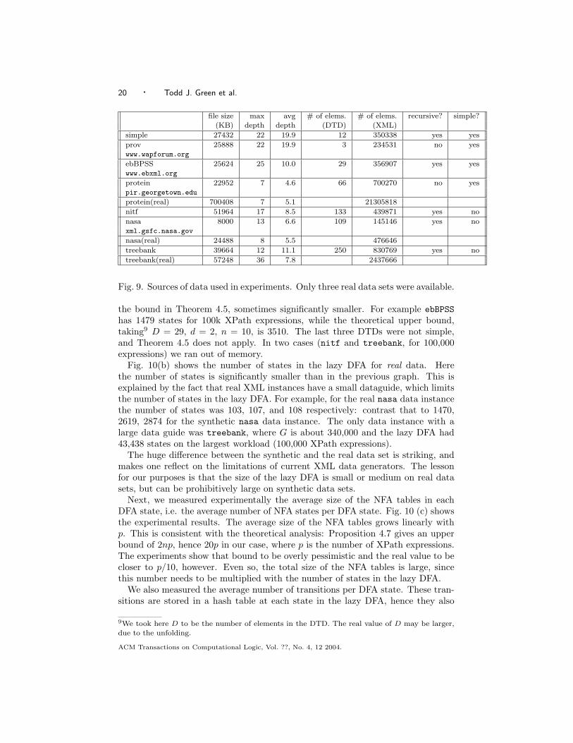
Fig. 10(a) shows the number of states in the lazy DFA on synthetic XML data.The first four DTDs are simple, and the number of states was indeed smaller than
ACM Transactions on Computational Logic, Vol. ??, No. 4, 12 2004.
20 · Todd J. Green et al.
file size max avg # of elems. # of elems. recursive? simple?(KB) depth depth (DTD) (XML)
simple 27432 22 19.9 12 350338 yes yes
prov 25888 22 19.9 3 234531 no yeswww.wapforum.org
ebBPSS 25624 25 10.0 29 356907 yes yeswww.ebxml.org
protein 22952 7 4.6 66 700270 no yes
pir.georgetown.edu
protein(real) 700408 7 5.1 21305818
nitf 51964 17 8.5 133 439871 yes no
nasa 8000 13 6.6 109 145146 yes noxml.gsfc.nasa.gov
nasa(real) 24488 8 5.5 476646
treebank 39664 12 11.1 250 830769 yes no
treebank(real) 57248 36 7.8 2437666
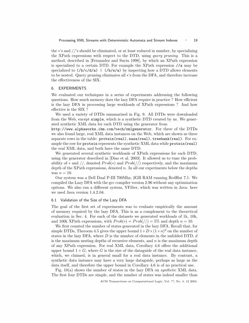
Fig. 9. Sources of data used in experiments. Only three real data sets were available.
the bound in Theorem 4.5, sometimes significantly smaller. For example ebBPSShas 1479 states for 100k XPath expressions, while the theoretical upper bound,taking9 D = 29, d = 2, n = 10, is 3510. The last three DTDs were not simple,and Theorem 4.5 does not apply. In two cases (nitf and treebank, for 100,000expressions) we ran out of memory.
Fig. 10(b) shows the number of states in the lazy DFA for real data. Herethe number of states is significantly smaller than in the previous graph. This isexplained by the fact that real XML instances have a small dataguide, which limitsthe number of states in the lazy DFA. For example, for the real nasa data instancethe number of states was 103, 107, and 108 respectively: contrast that to 1470,2619, 2874 for the synthetic nasa data instance. The only data instance with alarge data guide was treebank, where G is about 340,000 and the lazy DFA had43,438 states on the largest workload (100,000 XPath expressions).
The huge difference between the synthetic and the real data set is striking, andmakes one reflect on the limitations of current XML data generators. The lessonfor our purposes is that the size of the lazy DFA is small or medium on real datasets, but can be prohibitively large on synthetic data sets.
Next, we measured experimentally the average size of the NFA tables in eachDFA state, i.e. the average number of NFA states per DFA state. Fig. 10 (c) showsthe experimental results. The average size of the NFA tables grows linearly withp. This is consistent with the theoretical analysis: Proposition 4.7 gives an upperbound of 2np, hence 20p in our case, where p is the number of XPath expressions.The experiments show that bound to be overly pessimistic and the real value to becloser to p/10, however. Even so, the total size of the NFA tables is large, sincethis number needs to be multiplied with the number of states in the lazy DFA.
We also measured the average number of transitions per DFA state. These tran-sitions are stored in a hash table at each state in the lazy DFA, hence they also
9We took here D to be the number of elements in the DTD. The real value of D may be larger,due to the unfolding.
ACM Transactions on Computational Logic, Vol. ??, No. 4, 12 2004.
Processing XML Streams with Deterministic Automata and Stream Indexes · 21
1
10
100
1000
10000
100000
simple prov ebBPSS protein nasa nitf treebank
Number of DFA States - SYNTHETIC Data
1k XPEs10k XPEs100k XPEs
1
10
100
1000
10000
100000
protein (real) nasa (real) treebank (real)
Number of DFA States - REAL Data
1k XPEs
10k XPEs
100k XPEs
(a) (b)
Average NFA States per DFA state
1
10
100
1000
10000
100000
simple
prot
ein (r
eal)
prot
ein
nasa
(rea
l)na
sa
treeb
ank (
real)
treeb
ank
prov
ebBPSS nit
f
1k XPEs10k XPEs100k XPEs
Average Transitions per DFA State
1
10
100
1000
simple
prot
ein (r
eal)
prot
ein
nasa
(rea
l)na
sa
treeb
ank (
real)
treeb
ank
prov
ebBPSS nit
f
1k XPEs
10k XPEs
100k XPEs
(c) (d)
NFA/DFA MemoryUsage - REAL Data
0.1
1
10
100
1000
10000
protein(NFA)
protein(DFA)
NASA(NFA)
NASA(DFA)
treebank(NFA)
treebank(DFA)
MB
1k XPEs
10k XPEs
100k XPEs
(e)
Fig. 10. Size of the lazy DFA for synthetic data (a), and real data (b); average sizeof an NFA table (c), and of a transition table (d); total memory used by a lazyDFA (e). 1k XPEs means 1000 XPath expressions.
ACM Transactions on Computational Logic, Vol. ??, No. 4, 12 2004.
22 · Todd J. Green et al.
contribute to the total size. Notice that the number of transitions at a state isbounded by the number of elements in the DTD. Our experimental results in Fig. 10(d) confirm that. The transition tables are much smaller than the NFA tables.
Next we measured the total amount of memory used by the lazy DFA, expressedin MB’s.: this is shown in Fig. 10 (e). The most important observation is thatthe total amount of memory used by the lazy DFA grows largely linearly with thenumber of XPath expressions. This is explained by the fact that the number ofstates is largely invariant, while the average size of an NFA table at each stategrows linearly with the workload. We also measured the amount of memory usedby a naive NFA, without any of the state sharing optimization implemented inYFilter. The graph shows that this is comparable to the size of the lazy DFA.On one hand the total size of the NFA tables in the lazy DFA is larger than thenumber of states in the NFA, on the other hand the DFA makes up by having fewertransition tables.
None of the experiments above included any predicates on data values. To con-clude our evaluation of the memory usage of the lazy DFA, we measured the impactof predicates. Recall that the theoretical analysis for this case was done in Sec.4.3,and we refer to the notations in that section. We generated a workload of 200000XPath expressions with constant values. We used a subset of size 9.12MB of theprotein data set, and selected randomly constants that actually occur in this data.In order to select values randomly from this data instance we had to store the en-tire data in main memory. For that reason, we used only a subset of the proteindata set. The number of distinct constants used was q = 29740. The first tier ofthe automaton had 80 states (slightly less than Fig. 10 (b) because we used onlya fragment of the protein data), while the number of additional states was 63412states. That is, each distinct constant occurring in the predicates contributed toapproximatively two new states in the second tier of the automaton. The averagesize of the NFA tables at these states is at most as large as the average numberof XPath expressions containing each distinct constant, i.e. 200000/29740 ≈ 6.7.Since these states have no transition tables, each distinct value occurring in any ofthe predicates used about 13.4∗4 ≈ 54 bytes of main memory. While non-negligible,this amount is of the same order of magnitude as the predicate itself.
6.2 Throughput
In our second sets of experiments we measured the speed at which the lazy DFAprocesses the real XML data instances nasa and protein. Our first goal here wasto evaluate the speed of the lazy DFA during the stable phase, when most or all ofits states have been computed, and the lazy DFA reaches its maximum speed. Oursecond goal was to measure the length of the warmup phase, when most time isspent constructing new DFA states. To separate the warmup phase from the stablephase, we measured the instantaneous throughput, as a function of the amount ofXML data processed: we measured at 5MB intervals for nasa and 100MB intervalsfor protein, or more often when necessary.
We compared the lazy DFA to YFilter [Diao et al. 2003], a system that uses ahighly optimized NFA to evaluate large workloads of XPath expressions. Thereare many factors that make a direct comparison of the two systems difficult: theimplementation language (C++ for the lazy DFA v.s. Java for YFilter), the XMLACM Transactions on Computational Logic, Vol. ??, No. 4, 12 2004.
Processing XML Streams with Deterministic Automata and Stream Indexes · 23
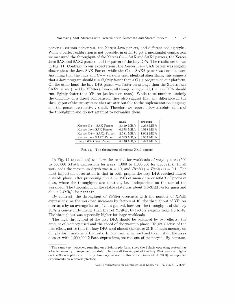
parser (a custom parser v.s. the Xerces Java parser), and different coding styles.While a perfect calibration is not possible, in order to get a meaningful comparisonwe measured the throughput of the Xerces C++ SAX and SAX2 parsers, the XercesJava SAX and SAX2 parsers, and the parser of the lazy DFA. The results are shownin Fig. 11. Contrary to our expectations, the Xerces C++ SAX parser was slightlyslower than the Java SAX Parser, while the C++ SAX2 parser was even slower.Assuming that the Java and C++ versions used identical algorithms, this suggeststhat a Java program should run slightly faster than a C++ program on our platform.On the other hand the lazy DFA parser was faster on average than the Xerces JavaSAX2 parser (used by YFilter), hence, all things being equal, the lazy DFA shouldrun slightly faster than YFilter (at least on nasa). While these numbers underlythe difficulty of a direct comparison, they also suggest that any difference in thethroughput of the two systems that are attributable to the implementation languageand the parser are relatively small. Therefore we report below absolute values ofthe throughput and do not attempt to normalize them.
nasa protein
Xerces C++ SAX Parser 5.449 MB/s 4.238 MB/sXerces Java SAX Parser 6.678 MB/s 6.518 MB/s
Xerces C++ SAX2 Parser 2.581 MB/s 1.902 MB/s
Xerces Java SAX2 Parser 6.663 MB/s 6.503 MB/s
Lazy DFA C++ Parser 8.476 MB/s 6.429 MB/s
Fig. 11. The throughput of various XML parsers.
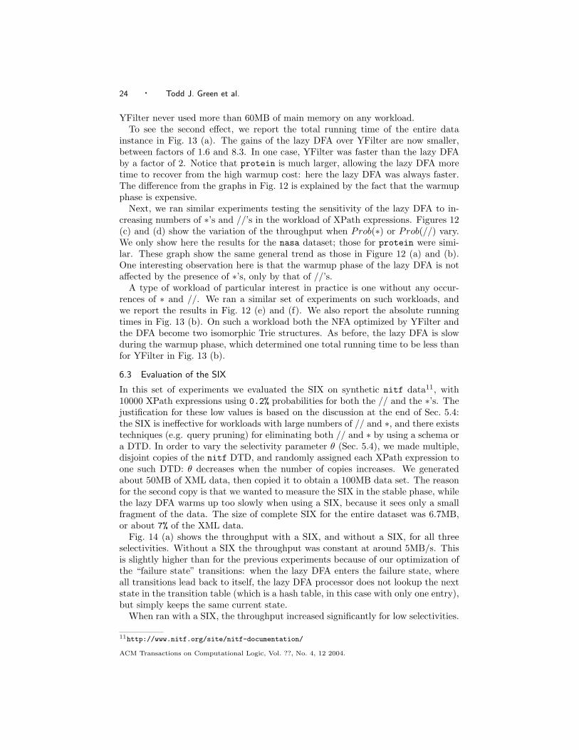
In Fig. 12 (a) and (b) we show the results for workloads of varying sizes (500to 500,000 XPath expressions for nasa, 1,000 to 1,000,000 for protein). In allworkloads the maximum depth was n = 10, and Prob(∗) = Prob(//) = 0.1. Themost important observation is that in both graphs the lazy DFA reached indeeda stable phase, after processing about 5-10MB of nasa data or 50MB of proteindata, where the throughput was constant, i.e. independent on the size of theworkload. The throughput in the stable state was about 3.3-3.4Mb/s for nasa andabout 2.4Mb/s for protein.
By contrast, the throughput of YFilter decreases with the number of XPathexpressions: as the workload increases by factors of 10, the throughput of YFilterdecreases by an average factor of 2. In general, however, the throughput of the lazyDFA is consistently higher than that of YFilter, by factors ranging from 4.6 to 48.The throughput was especially higher for large workloads.
The high throughput of the lazy DFA should be balanced by two effects: theamount of memory used and the speed of the warmup phase. To get a sense of thefirst effect, notice that the lazy DFA used almost the entire 2GB of main memory onour platform in some of the tests. In one case, when we tried to run it on the nasadataset with 1,000,000 XPath expressions, we ran out of memory10. By contrast,
10The same test, however, runs fine on a Solaris platform, since the Solaris operating system has
a better memory management module. The overall throughput of the lazy DFA was also higheron the Solaris platform. In a preliminary version of this work [Green et al. 2003] we reported
experiments on a Solaris platform.
ACM Transactions on Computational Logic, Vol. ??, No. 4, 12 2004.
24 · Todd J. Green et al.
YFilter never used more than 60MB of main memory on any workload.To see the second effect, we report the total running time of the entire data
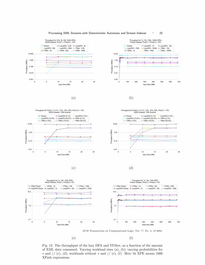
instance in Fig. 13 (a). The gains of the lazy DFA over YFilter are now smaller,between factors of 1.6 and 8.3. In one case, YFilter was faster than the lazy DFAby a factor of 2. Notice that protein is much larger, allowing the lazy DFA moretime to recover from the high warmup cost: here the lazy DFA was always faster.The difference from the graphs in Fig. 12 is explained by the fact that the warmupphase is expensive.
Next, we ran similar experiments testing the sensitivity of the lazy DFA to in-creasing numbers of ∗’s and //’s in the workload of XPath expressions. Figures 12(c) and (d) show the variation of the throughput when Prob(∗) or Prob(//) vary.We only show here the results for the nasa dataset; those for protein were simi-lar. These graph show the same general trend as those in Figure 12 (a) and (b).One interesting observation here is that the warmup phase of the lazy DFA is notaffected by the presence of ∗’s, only by that of //’s.
A type of workload of particular interest in practice is one without any occur-rences of ∗ and //. We ran a similar set of experiments on such workloads, andwe report the results in Fig. 12 (e) and (f). We also report the absolute runningtimes in Fig. 13 (b). On such a workload both the NFA optimized by YFilter andthe DFA become two isomorphic Trie structures. As before, the lazy DFA is slowduring the warmup phase, which determined one total running time to be less thanfor YFilter in Fig. 13 (b).
6.3 Evaluation of the SIX
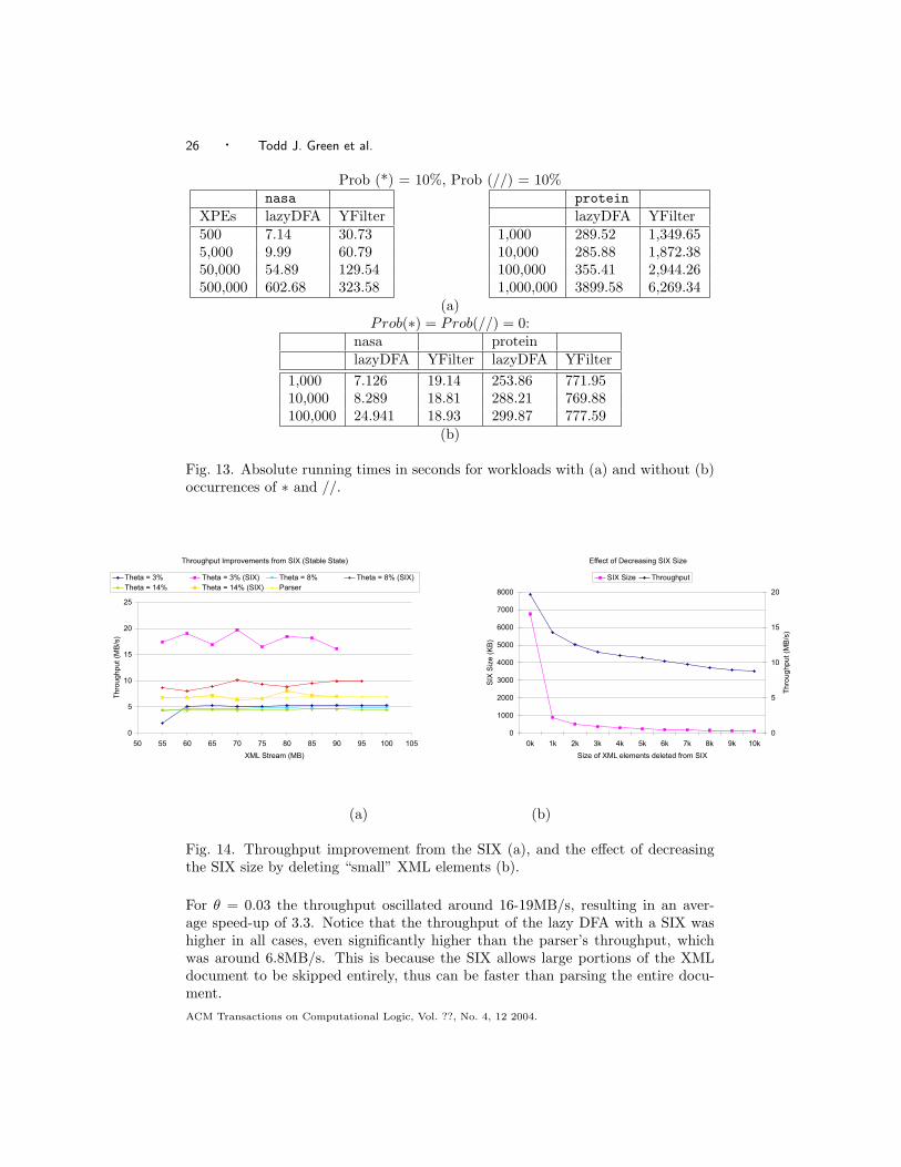
In this set of experiments we evaluated the SIX on synthetic nitf data11, with10000 XPath expressions using 0.2% probabilities for both the // and the ∗’s. Thejustification for these low values is based on the discussion at the end of Sec. 5.4:the SIX is ineffective for workloads with large numbers of // and ∗, and there existstechniques (e.g. query pruning) for eliminating both // and ∗ by using a schema ora DTD. In order to vary the selectivity parameter θ (Sec. 5.4), we made multiple,disjoint copies of the nitf DTD, and randomly assigned each XPath expression toone such DTD: θ decreases when the number of copies increases. We generatedabout 50MB of XML data, then copied it to obtain a 100MB data set. The reasonfor the second copy is that we wanted to measure the SIX in the stable phase, whilethe lazy DFA warms up too slowly when using a SIX, because it sees only a smallfragment of the data. The size of complete SIX for the entire dataset was 6.7MB,or about 7% of the XML data.
Fig. 14 (a) shows the throughput with a SIX, and without a SIX, for all threeselectivities. Without a SIX the throughput was constant at around 5MB/s. Thisis slightly higher than for the previous experiments because of our optimization ofthe “failure state” transitions: when the lazy DFA enters the failure state, whereall transitions lead back to itself, the lazy DFA processor does not lookup the nextstate in the transition table (which is a hash table, in this case with only one entry),but simply keeps the same current state.
When ran with a SIX, the throughput increased significantly for low selectivities.
11http://www.nitf.org/site/nitf-documentation/
ACM Transactions on Computational Logic, Vol. ??, No. 4, 12 2004.
Processing XML Streams with Deterministic Automata and Stream Indexes · 25
Throughput for 0.5k, 5k, 50k, 500k XPEsNASA Dataset, Prob(*) = Prob(//) = 10%
0.001
0.010
0.100
1.000
10.000
0 5 10 15 20 25
Input Size (MB)
Thr
ough
put (
MB
/s)
Parser LazyDFA - 0.5k LazyDFA - 5kLazyDFA - 50k LazyDFA - 500k Yfilter - 0.5kYfilter - 5k Yfilter - 50k Yfilter - 500k
Throughput for 1k, 10k, 100k, 1000k XPEsProtein Dataset, Prob(*) = Prob(//) = 10%
0.00
0.01
0.10
1.00
10.00
0 100 200 300 400 500 600 700
Input Size (MB)
Thr
ough
put (
MB
/s)
Parser LazyDFA - 1k LazyDFA - 10kLazyDFA - 100k LazyDFA - 1000k Yfilter - 10kYfilter - 1k Yfilter - 100k Yfilter - 1000k
(a) (b)
Throughput for Prob(*) = 0.1%, 1.0%, 10%, 50%, Prob (//) = 10%NASA Dataset, 100k Queries
0.01
0.10
1.00
10.00
0 5 10 15 20 25
Input Size (MB)
Thr
ough
put (
MB
/s)
Parser LazyDFA (0.1%) LazyDFA (1.0%)LazyDFA (10.0%) LazyDFA (50.0%) Yfilter (0.1%)Yfilter (1.0%) Yfilter (10.0%) Yfilter (50.0%)
Throughput for Prob(//) = 0.1%, 1.0%, 10%, 50%, Prob(*) = 10%NASA Dataset, 100k Queries
0.01
0.10
1.00
10.00
0 5 10 15 20 25
Input Size (MB)
Thr
ough
put (
MB
/s)
Parser LazyDFA (0.1%) LazyDFA (1.0%)LazyDFA (10.0%) LazyDFA (50.0%) Yfilter (0.1%)Yfilter (1.0%) Yfilter (10.0%) Yfilter (50.0%)
(c) (d)
Throughput for 1k, 10k, 100k XPEsNASA Dataset, Prob(*) = Prob(//) = 0%
0.1
1.0
10.0
0 5 10 15 20 25
Data Size (MB)
Thr
ough
put (
MB
/s)
Yfilter Parser YFilter - 1k YFilter - 10k YFilter - 100kLazyDFA Parser LazyDFA - 1k LazyDFA - 10k LazyDFA - 100K
Throughput for 1k, 10k, 100k XPEsProtein Dataset, Prob(*) = Prob(//) = 0%
0.1
1.0
10.0
0 100 200 300 400 500 600 700
Data Size (MB)
Thr
ough
put (
MB
/s)
Yfilter Parser YFilter - 1k YFilter -10k YFilter -100kLazyDFA Parser LazyDFA - 1k LazyDFA - 10k LazyDFA - 100k
(e) (f)
Fig. 12. The throughput of the lazy DFA and YFilter, as a function of the amountof XML data consumed. Varying workload sizes (a), (b); varying probabilities for∗ and // (c), (d); workloads without ∗ and // (e), (f). Here 1k XPE means 1000XPath expressions.
ACM Transactions on Computational Logic, Vol. ??, No. 4, 12 2004.
26 · Todd J. Green et al.
Prob (*) = 10%, Prob (//) = 10%nasa
XPEs lazyDFA YFilter500 7.14 30.735,000 9.99 60.7950,000 54.89 129.54500,000 602.68 323.58
proteinlazyDFA YFilter
1,000 289.52 1,349.6510,000 285.88 1,872.38100,000 355.41 2,944.261,000,000 3899.58 6,269.34
(a)Prob(∗) = Prob(//) = 0:
nasa proteinlazyDFA YFilter lazyDFA YFilter
1,000 7.126 19.14 253.86 771.9510,000 8.289 18.81 288.21 769.88100,000 24.941 18.93 299.87 777.59
(b)
Fig. 13. Absolute running times in seconds for workloads with (a) and without (b)occurrences of ∗ and //.
Throughput Improvements from SIX (Stable State)
0
5
10
15
20
25
50 55 60 65 70 75 80 85 90 95 100 105
XML Stream (MB)
Thr
ough
put (
MB
/s)
Theta = 3% Theta = 3% (SIX) Theta = 8% Theta = 8% (SIX)Theta = 14% Theta = 14% (SIX) Parser
Effect of Decreasing SIX Size
0
1000
2000
3000
4000
5000
6000
7000
8000
0k 1k 2k 3k 4k 5k 6k 7k 8k 9k 10k
Size of XML elements deleted from SIX
SIX
Siz
e (K
B)
0
5
10
15
20
Thr
ough
put (
MB
/s)
SIX Size Throughput
(a) (b)
Fig. 14. Throughput improvement from the SIX (a), and the effect of decreasingthe SIX size by deleting “small” XML elements (b).
For θ = 0.03 the throughput oscillated around 16-19MB/s, resulting in an aver-age speed-up of 3.3. Notice that the throughput of the lazy DFA with a SIX washigher in all cases, even significantly higher than the parser’s throughput, whichwas around 6.8MB/s. This is because the SIX allows large portions of the XMLdocument to be skipped entirely, thus can be faster than parsing the entire docu-ment.ACM Transactions on Computational Logic, Vol. ??, No. 4, 12 2004.
Processing XML Streams with Deterministic Automata and Stream Indexes · 27
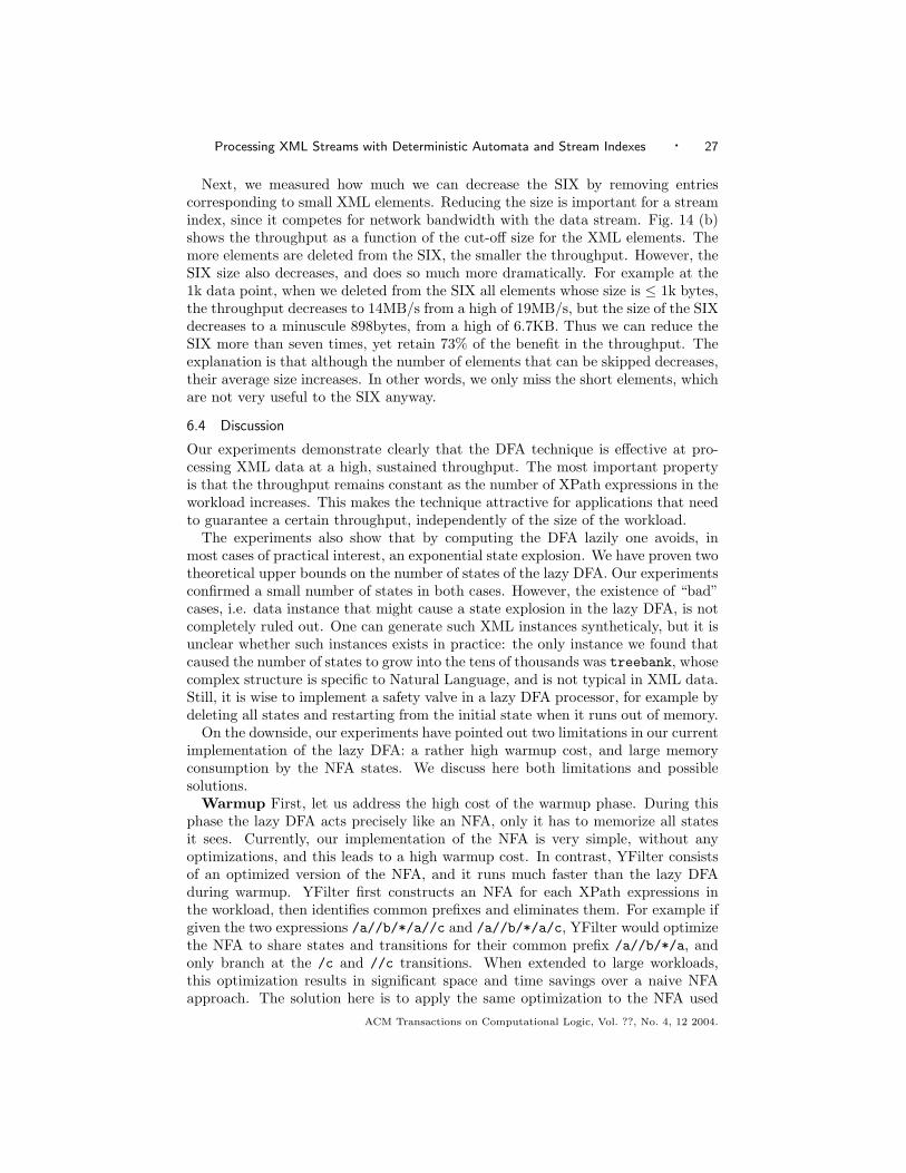
Next, we measured how much we can decrease the SIX by removing entriescorresponding to small XML elements. Reducing the size is important for a streamindex, since it competes for network bandwidth with the data stream. Fig. 14 (b)shows the throughput as a function of the cut-off size for the XML elements. Themore elements are deleted from the SIX, the smaller the throughput. However, theSIX size also decreases, and does so much more dramatically. For example at the1k data point, when we deleted from the SIX all elements whose size is ≤ 1k bytes,the throughput decreases to 14MB/s from a high of 19MB/s, but the size of the SIXdecreases to a minuscule 898bytes, from a high of 6.7KB. Thus we can reduce theSIX more than seven times, yet retain 73% of the benefit in the throughput. Theexplanation is that although the number of elements that can be skipped decreases,their average size increases. In other words, we only miss the short elements, whichare not very useful to the SIX anyway.
6.4 Discussion
Our experiments demonstrate clearly that the DFA technique is effective at pro-cessing XML data at a high, sustained throughput. The most important propertyis that the throughput remains constant as the number of XPath expressions in theworkload increases. This makes the technique attractive for applications that needto guarantee a certain throughput, independently of the size of the workload.
The experiments also show that by computing the DFA lazily one avoids, inmost cases of practical interest, an exponential state explosion. We have proven twotheoretical upper bounds on the number of states of the lazy DFA. Our experimentsconfirmed a small number of states in both cases. However, the existence of “bad”cases, i.e. data instance that might cause a state explosion in the lazy DFA, is notcompletely ruled out. One can generate such XML instances syntheticaly, but it isunclear whether such instances exists in practice: the only instance we found thatcaused the number of states to grow into the tens of thousands was treebank, whosecomplex structure is specific to Natural Language, and is not typical in XML data.Still, it is wise to implement a safety valve in a lazy DFA processor, for example bydeleting all states and restarting from the initial state when it runs out of memory.
On the downside, our experiments have pointed out two limitations in our currentimplementation of the lazy DFA: a rather high warmup cost, and large memoryconsumption by the NFA states. We discuss here both limitations and possiblesolutions.
Warmup First, let us address the high cost of the warmup phase. During thisphase the lazy DFA acts precisely like an NFA, only it has to memorize all statesit sees. Currently, our implementation of the NFA is very simple, without anyoptimizations, and this leads to a high warmup cost. In contrast, YFilter consistsof an optimized version of the NFA, and it runs much faster than the lazy DFAduring warmup. YFilter first constructs an NFA for each XPath expressions inthe workload, then identifies common prefixes and eliminates them. For example ifgiven the two expressions /a//b/*/a//c and /a//b/*/a/c, YFilter would optimizethe NFA to share states and transitions for their common prefix /a//b/*/a, andonly branch at the /c and //c transitions. When extended to large workloads,this optimization results in significant space and time savings over a naive NFAapproach. The solution here is to apply the same optimization to the NFA used
ACM Transactions on Computational Logic, Vol. ??, No. 4, 12 2004.
28 · Todd J. Green et al.
by the lazy DFA. It suffices to replace the currently naive NFA with YFilter’soptimized NFA, and leave the rest of the lazy DFA unchanged. This would speedup the warmup phase considerably, making it comparable to YFilter, and wouldnot affect the throughput in the stable phase.
With or without optimizations, the manipulation of the NFA tables is expensive,and we have put a lot of thought into their implementation. There are threeoperations done on NFA tables: create, insert, and compare. To illustrate theircomplexity, consider an example where the lazy DFA ends up having 10,000 states,each with an NFA table with 30,000 entries, and that the alphabet Σ has 50 symbols.Then, during warm-up phase we need to create 50 × 10, 000 = 500, 000 new sets;insert 30, 000 NFA states in each set; and compare, on average, 500, 000×10, 000/2pairs of sets, of which only 490,000 comparisons return true, the others returnfalse. We found that implementing sets as sorted arrays of pointers offered thebest overall performance. An insertion takes O(1) time, because we insert at theend, and sort the array when we finish all insertions. We compute a hash value(signature) for each array, thus comparisons with negative answers take O(1) invirtually all cases.
Memory Second, we will discuss the high memory consumption of the lazy DFA.As our experiments show, this is due to the NFA tables, not the number of states inthe lazy DFA. There are several possible approaches to address this, but studyingtheir effectiveness remains part of future work. The simplest one is to adopt theYFilter optimizations as explained above: in addition to speeding up the warmupphase this can also decrease the average size of the NFA tables. A second is todelete the NFA tables from “completed” DFA states. A completed DFA state isone in which all its transitions have already been expanded. The NFA table in aDFA state is only needed when a new transition is followed, in order to constructthe new destination DFA state. Once all such transitions have been expanded,there is no more need for the NFA table.
We notice however that, when run on smaller workloads, the lazy DFA uses farless memory than many other systems. Peng and Chwawathe [Peng and Chawathe2003] evaluate the throughput and the memory usage of seven systems, includingthe XML Toolkit (which is based on the lazy DFA and is described here in Sec. 7).In their evaluation the XML Toolkit used by far the least amount of memory, somecases by several orders of magnitude.
Finally, we discuss here the effectiveness of the SIX. Like with any index, it onlybenefits queries or workloads that retrieve only a very small portion of the data.Our experiments showed the SIX to be effective for workload of 10,000, but on adataset where we decreased the selectivity artificially. In order to use the SIX in anapplication like XML packet routine, one needs to cluster XPath expressions intoworkloads in order to reduce the θ factor for each workload. When this is possible,then the SIX can be very effective.
7. AN APPLICATION: THE XML TOOLKIT (XMLTK)
We describe here an application of our XPath processing techniques, to a set of toolsfor highly performant processing of large XML files. The XML Toolkit is modeledafter the Unix tools for processing text files, and is available at http://xmltk.sourceforge.net.ACM Transactions on Computational Logic, Vol. ??, No. 4, 12 2004.
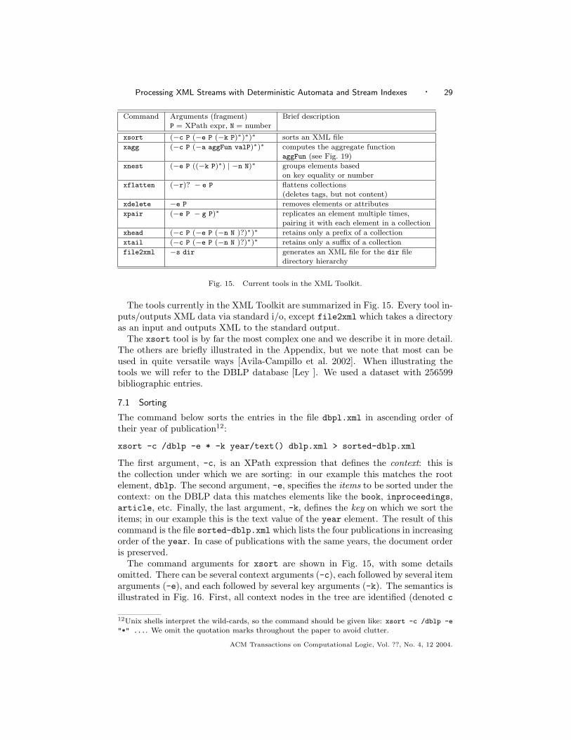
Processing XML Streams with Deterministic Automata and Stream Indexes · 29
Command Arguments (fragment) Brief description
P = XPath expr, N = number
xsort (−c P (−e P (−k P)∗)∗)∗ sorts an XML file
xagg (−c P (−a aggFun valP)∗)∗ computes the aggregate functionaggFun (see Fig. 19)
xnest (−e P ((−k P)∗) | −n N)∗ groups elements based
on key equality or number
xflatten (−r)? − e P flattens collections(deletes tags, but not content)
xdelete −e P removes elements or attributes
xpair (−e P − g P)∗ replicates an element multiple times,pairing it with each element in a collection
xhead (−c P (−e P (−n N )?)∗)∗ retains only a prefix of a collection
xtail (−c P (−e P (−n N )?)∗)∗ retains only a suffix of a collection
file2xml −s dir generates an XML file for the dir file
directory hierarchy
Fig. 15. Current tools in the XML Toolkit.
The tools currently in the XML Toolkit are summarized in Fig. 15. Every tool in-puts/outputs XML data via standard i/o, except file2xml which takes a directoryas an input and outputs XML to the standard output.
The xsort tool is by far the most complex one and we describe it in more detail.The others are briefly illustrated in the Appendix, but we note that most can beused in quite versatile ways [Avila-Campillo et al. 2002]. When illustrating thetools we will refer to the DBLP database [Ley ]. We used a dataset with 256599bibliographic entries.
7.1 Sorting
The command below sorts the entries in the file dbpl.xml in ascending order oftheir year of publication12:
xsort -c /dblp -e * -k year/text() dblp.xml > sorted-dblp.xml
The first argument, -c, is an XPath expression that defines the context: this isthe collection under which we are sorting: in our example this matches the rootelement, dblp. The second argument, -e, specifies the items to be sorted under thecontext: on the DBLP data this matches elements like the book, inproceedings,article, etc. Finally, the last argument, -k, defines the key on which we sort theitems; in our example this is the text value of the year element. The result of thiscommand is the file sorted-dblp.xml which lists the four publications in increasingorder of the year. In case of publications with the same years, the document orderis preserved.
The command arguments for xsort are shown in Fig. 15, with some detailsomitted. There can be several context arguments (-c), each followed by several itemarguments (-e), and each followed by several key arguments (-k). The semantics isillustrated in Fig. 16. First, all context nodes in the tree are identified (denoted c
12Unix shells interpret the wild-cards, so the command should be given like: xsort -c /dblp -e
"*" .... We omit the quotation marks throughout the paper to avoid clutter.
ACM Transactions on Computational Logic, Vol. ??, No. 4, 12 2004.
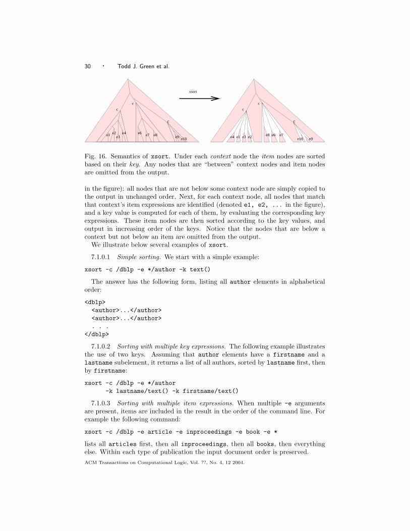
30 · Todd J. Green et al.
c
c
c
e3e4 e2e1 e8 e7e6e10 e9
c
c
c
e1 e2e3
e4 e6 e7 e8 e9 e10
xsort
Fig. 16. Semantics of xsort. Under each context node the item nodes are sortedbased on their key. Any nodes that are “between” context nodes and item nodesare omitted from the output.
in the figure): all nodes that are not below some context node are simply copied tothe output in unchanged order. Next, for each context node, all nodes that matchthat context’s item expressions are identified (denoted e1, e2, ... in the figure),and a key value is computed for each of them, by evaluating the corresponding keyexpressions. These item nodes are then sorted according to the key values, andoutput in increasing order of the keys. Notice that the nodes that are below acontext but not below an item are omitted from the output.
We illustrate below several examples of xsort.
7.1.0.1 Simple sorting. We start with a simple example:
xsort -c /dblp -e */author -k text()
The answer has the following form, listing all author elements in alphabeticalorder:
<dblp><author>...</author><author>...</author>. . .
</dblp>
7.1.0.2 Sorting with multiple key expressions. The following example illustratesthe use of two keys. Assuming that author elements have a firstname and alastname subelement, it returns a list of all authors, sorted by lastname first, thenby firstname:
xsort -c /dblp -e */author-k lastname/text() -k firstname/text()
7.1.0.3 Sorting with multiple item expressions. When multiple -e argumentsare present, items are included in the result in the order of the command line. Forexample the following command:
xsort -c /dblp -e article -e inproceedings -e book -e *
lists all articles first, then all inproceedings, then all books, then everythingelse. Within each type of publication the input document order is preserved.ACM Transactions on Computational Logic, Vol. ??, No. 4, 12 2004.
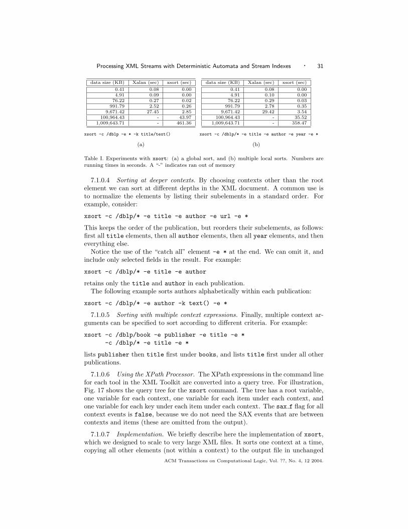
Processing XML Streams with Deterministic Automata and Stream Indexes · 31
data size (KB) Xalan (sec) xsort (sec)
0.41 0.08 0.004.91 0.09 0.00
76.22 0.27 0.02991.79 2.52 0.26
9,671.42 27.45 2.85100,964.43 - 43.97
1,009,643.71 - 461.36
xsort -c /dblp -e * -k title/text()
(a)
data size (KB) Xalan (sec) xsort (sec)
0.41 0.08 0.004.91 0.10 0.00
76.22 0.29 0.03991.79 2.78 0.35
9,671.42 29.42 3.54100,964.43 - 35.52
1,009,643.71 - 358.47
xsort -c /dblp/* -e title -e author -e year -e *
(b)
Table I. Experiments with xsort: (a) a global sort, and (b) multiple local sorts. Numbers are
running times in seconds. A “-” indicates ran out of memory
7.1.0.4 Sorting at deeper contexts. By choosing contexts other than the rootelement we can sort at different depths in the XML document. A common use isto normalize the elements by listing their subelements in a standard order. Forexample, consider:
xsort -c /dblp/* -e title -e author -e url -e *
This keeps the order of the publication, but reorders their subelements, as follows:first all title elements, then all author elements, then all year elements, and theneverything else.
Notice the use of the “catch all” element -e * at the end. We can omit it, andinclude only selected fields in the result. For example:
xsort -c /dblp/* -e title -e author
retains only the title and author in each publication.The following example sorts authors alphabetically within each publication:
xsort -c /dblp/* -e author -k text() -e *
7.1.0.5 Sorting with multiple context expressions. Finally, multiple context ar-guments can be specified to sort according to different criteria. For example:
xsort -c /dblp/book -e publisher -e title -e *-c /dblp/* -e title -e *
lists publisher then title first under books, and lists title first under all otherpublications.
7.1.0.6 Using the XPath Processor. The XPath expressions in the command linefor each tool in the XML Toolkit are converted into a query tree. For illustration,Fig. 17 shows the query tree for the xsort command. The tree has a root variable,one variable for each context, one variable for each item under each context, andone variable for each key under each item under each context. The sax f flag for allcontext events is false, because we do not need the SAX events that are betweencontexts and items (these are omitted from the output).
7.1.0.7 Implementation. We briefly describe here the implementation of xsort,which we designed to scale to very large XML files. It sorts one context at a time,copying all other elements (not within a context) to the output file in unchanged
ACM Transactions on Computational Logic, Vol. ??, No. 4, 12 2004.
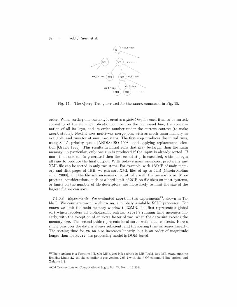
32 · Todd J. Green et al.
. . . . . .
$E1 $E2
$K1
$R
$C1 $C2
$K2
. . . . . .
. . . . . .
sax_f = true
sax_f = truesax_f = true
sax_f = true sax_f = true
Fig. 17. The Query Tree generated for the xsort command in Fig. 15.
order. When sorting one context, it creates a global key for each item to be sorted,consisting of the item identification number on the command line, the concate-nation of all its keys, and its order number under the current context (to makexsort stable). Next it uses multi-way merge-join, with as much main memory asavailable, and runs for at most two steps. The first step produces the initial runs,using STL’s priority queue [ANDIS/ISO 1998], and applying replacement selec-tion [Graefe 1993]. This results in initial runs that may be larger than the mainmemory: in particular, only one run is produced if the input is already sorted. Ifmore than one run is generated then the second step is executed, which mergesall runs to produce the final output. With today’s main memories, practically anyXML file can be sorted in only two steps. For example, with 128MB of main mem-ory and disk pages of 4KB, we can sort XML files of up to 4TB [Garcia-Molinaet al. 2000], and the file size increases quadratically with the memory size. Morepractical considerations, such as a hard limit of 2GB on file sizes on most systems,or limits on the number of file descriptors, are more likely to limit the size of thelargest file we can sort.
7.1.0.8 Experiments. We evaluated xsort in two experiments13, shown in Ta-ble I. We compare xsort with xalan, a publicly available XSLT processor. Forxsort we limit the main memory window to 32MB. The first represents a globalsort which reorders all bibliographic entries: xsort’s running time increases lin-early, with the exception of an extra factor of two, when the data size exceeds thememory size. The second table represents local sorts, with small contexts. Here asingle pass over the data is always sufficient, and the sorting time increases linearly.The sorting time for xalan also increases linearly, but is an order of magnitudelonger than for xsort. Its processing model is DOM-based.
13The platform is a Pentium III, 800 MHz, 256 KB cache 128 MB RAM, 512 MB swap, runningRedHat Linux 2.2.18, the compiler is gcc version 2.95.2 with the “-O” command-line option, and
Xalan-c 1.3.
ACM Transactions on Computational Logic, Vol. ??, No. 4, 12 2004.
Processing XML Streams with Deterministic Automata and Stream Indexes · 33
8. RELATED WORK
The problem of evaluating large collections of XPath expressions on a stream ofXML documents was first introduced in [Altinel and Franklin 2000], for a publish-subscribe system called XFilter. Improved techniques have been discussed in XTrie [Chanet al. 2002] (based on a trie), our preliminary version of this work [Green et al. 2003](based on lazy DFAs), and YFilter [Diao et al. 2003] (based on optimized NFAs). Inall methods, except ours, there is a space guarantee that is proportional to the totalsize of all XPath expressions in the workload, but no guarantee on the throughput.Our method makes the opposite tradeoff.
Two optimizations of the lazy DFA are described in [Onizuka 2003]. In one,the XPath expressions are clustered according to their axis types (/ or //) at eachdepth level. This is shown to reduce the number of DFA states: for example, it isshown that by clustering into 8 DFAs, memory usage decreases by a factor of 40and throughput only by a factor of 8. In the other optimization, NFA tables areallowed to share common subsets, thus saving memory.
More recently, some systems have been described that process more complexXPath expressions [Peng and Chawathe 2003; Gupta and Suciu 2003], or fragmentsof XQuery [Ludaescher et al. 2002; Diao and Franklin 2003]. A complete XQueryengine for streaming data is described in [Florescu et al. 2003].
A related problem is the event detection problem described in [Nguyen et al.2001]. Each event is a set of atomic events, and they trigger queries defined byother sets of events. The technique used here is also a variation on the Trie datastructure.
Ives et al. [Ives et al. 2002] describe a general-purpose XML query processorthat, at the lowest level, uses an event based processing model, and show howsuch a model can be integrated with a highly optimized XML query processor.We were influenced by [Ives et al. 2002] in designing our stream processing model.Query processors like [Ives et al. 2002] can benefit from an efficient low-level streamprocessor. Specializing regular expressions w.r.t. schemas is described in [Fernandezand Suciu 1998; McHugh and Widom 1999].
The conversion problem from regular expression to an NFA has been intensivelystudied in the 60s and 70s: see [Watson 1993] for a review. The most popularmethods is due to Thompson [Thompson 1968] and is adopted by most textbooks.
Empirical studies of the (eager) DFA construction time have been done in theautomaton community [Watson 1996], for NFAs with up to 30 to 50 states.
9. CONCLUSION
We have described two techniques for processing linear XPath expressions on streamsof XML packets: using a Deterministic Finite Automaton, and a Stream IndeX(SIX). The main problem with the DFA is that the worst case memory requirementis exponential in the size of the XPath workload. We have presented a combinationof theoretical results and experimental validations that together prove that the sizeof the lazy DFA remains small, for all practical purposes. Some of the theoreticalresults offer insights into the structure of XPath expressions that is of independentinterest. We also validated lazy DFAs on streaming XML data and shown thatthey indeed have a very high throughput, which is independent on the number of
ACM Transactions on Computational Logic, Vol. ??, No. 4, 12 2004.
34 · Todd J. Green et al.
XPath expressions in the workload. The SIX is a simple technique that adds somesmall amount of binary data to an XML document, which helps speed up a queryprocessor by several factors. Finally, we described a simple application of theseXPath processing techniques: the XML Toolkit, a collection of command-line toolsfor highly scalable XML data processing.
Electronic Appendix The electronic appendix for this article can be accessedin the ACM Digital Library. The appendix contains the proofs of many theoremsfrom the main body of the article, and a description of several tools in the XMLtoolkit.
Acknowledgment We thank Peter Buneman, AnHai Doan, Zack Ives, and Ar-naud Sahuguet for their comments on earlier versions of this paper. We also thankIliana Avila-Campillo, Yana Kadiyska, Jason Kim, and Demian Raven for theircontributions to the XML Toolkit, Cristine Haertl for pointing out a bug in thesecond example in Fig. 6 and suggesting the fix, and the anonymous reviewers fortheir useful comments. Suciu was partially supported by the NSF CAREER GrantIIS-0092955, NSF Grants IIS-0140493 and IIS-0205635, a gift from Microsoft, anda Sloan Fellowship.
REFERENCES
Abiteboul, S., Buneman, P., and Suciu, D. 1999. Data on the Web : From Relations to
Semistructured Data and XML. Morgan Kaufmann.
Aho, A. and Corasick, M. 1975. Efficient string matching: an aid to bibliographic search.Communications of the ACM 18, 333–340.
Altinel, M. and Franklin, M. 2000. Efficient filtering of XML documents for selective dissem-ination. In Proceedings of VLDB. Cairo, Egipt, 53–64.
ANDIS/ISO 1998. C++ Standard. ANDIS/ISO.
Avila-Campillo, I., Green, T. J., Gupta, A., Onizuka, M., Raven, D., and Suciu, D. 2002.
XMLTK: An XML toolkit for scalable XML stream processing. In Proceedings of PLANX.
Borne, K. D. NASA’s astronomical data center. ADC XML resource page.http://xml.gsfc.nasa.gov/.
Buneman, P., Davidson, S., Fernandez, M., and Suciu, D. 1997. Adding structure to un-
structured data. In Proceedings of the International Conference on Database Theory. SpringerVerlag, Deplhi, Greece, 336–350.
Buneman, P., Naqvi, S. A., Tannen, V., and Wong, L. 1995. Principles of programming withcomplex objects and collection types. Theoretical Computer Science 149, 1, 3–48.
Chan, C., Felber, P., Garofalakis, M., and Rastogi, R. 2002. Efficient filtering of XML
documents with XPath expressions. In Proceedings of the International Conference on DataEngineering.
Chen, J., DeWitt, D., Tian, F., and Wang, Y. 2000. NiagaraCQ: a scalable continuous querysystem for internet databases. In Proceedings of the ACM/SIGMOD Conference on Manage-
ment of Data. 379–390.
Cormen, T. H., Leiserson, C. E., and Rivest, R. L. 1990. Introduction to Algorithms. MITPress.
Corp., M. DIME - direct internet message encapsulation spec-ification index page. IETF Internet Draft, available fromhttp://msdn.microsoft.com/webservices/understanding/gxa/default.aspx.
Diao, Y., Altinel, M., Franklin, M., Zhang, H., and Fischer, P. 2003. Path sharing andpredicate evaluation for high-performance XML filtering. ACM Transations on Database Sys-
tems 28, 4, 467–516.
Diao, Y. and Franklin, M. 2003. Query processing for high-volume XML message brokering.
In Proceedings of VLDB. Berlin, Germany.
ACM Transactions on Computational Logic, Vol. ??, No. 4, 12 2004.
Processing XML Streams with Deterministic Automata and Stream Indexes · 35
Fernandez, M. and Suciu, D. 1998. Optimizing regular path expressions using graph schemas.
In Proceedings of the International Conference on Data Engineering. 14–23.
Florescu, D., Hillary, C., Kossmann, D., P.Lucas, Riccardi, F., Westmann, T., Carey,M., Sundararajan, A., and Agrawal, G. 2003. The bea/xqrl streaming xquery processor. In
VLDB. Berlin, Germany, 997–1008.
Garcia-Molina, H., Ullman, J. D., and Widom, J. 2000. Database System Implementation.
Prentice Hall, Upper Saddle River, New Jersey 07458.
Goldman, R. and Widom, J. 1997. DataGuides: enabling query formulation and optimization
in semistructured databases. In Proceedings of Very Large Data Bases. 436–445.
Graefe, G. 1993. Query evaluation techniques for large databases. ACM Computing Sur-
veys 25, 2 (June), 73–170.
Green, T. J., Miklau, G., Onizuka, M., and Suciu, D. 2003. Processing XML streams withdeterministic automata. In Proceedings of ICDT. 173–189.
Gupta, A., Halevy, A., and Suciu, D. 2002. View selection for XML stream processing. In
WebDB.
Gupta, A. and Suciu, D. 2003. Stream processing of XPath queries with predicates. In Proceedingof ACM SIGMOD Conference on Management of Data.
Gupta, A., Suciu, D., and Halevy, A. 2003. The view selection problem for XML content based
routing. In Proceeding of PODS.
Higgins, D. G., Fuchs, R., Stoehr, P. J., and Cameron, G. N. 1992. The EMBL data library.
Nucleic Acids Research 20, 2071–2074.
Hopcroft, J. and Ullman, J. 1979. Introduction to automata theory, languages, and computa-tion. Addison-Wesley.
Ives, Z., Halevy, A., and Weld, D. 2002. An XML query engine for network-bound data.
VLDB Journal 11, 4, 380–402.
Laurikari, V. 2000. Nfas with tagged transitions, their conversion to deterministic automataand application to regular expressions. In Proceedings of SPIRE. 181–187.
Ley, M. Computer science bibliography (dblp). http://dblp.uni-trier.de.
Liefke, H. and Suciu, D. 2000. XMill: an efficent compressor for XML data. In Proceedings of
SIGMOD. Dallas, TX, 153–164.
Ludaescher, B., Mukhopadhyay, P., and Papakonstantinou, Y. 2002. A transducer-based
XML query processor. In Proceedings of VLDB. 227–238.
Marcus, M., Santorini, B., and M.A.Marcinkiewicz. 1993. Building a large annotated corpus
of English: the Penn Treenbak. Computational Linguistics 19.
McHugh, J. and Widom, J. 1999. Query optimization for XML. In Proceedings of VLDB.
Edinburgh, UK, 315–326.
Nguyen, B., Abiteboul, S., Cobena, G., and Preda, M. 2001. Monitoring XML data on theweb. In Proceedings of the ACM SIGMOD Conference on Management of Data. Santa Barbara,
437–448.
Onizuka, M. 2003. Light-weight xpath processing of XML stream with deterministic automata.
In Proc. CIKM. 342–349.
Peng, F. and Chawathe, S. 2003. XPath queries on streaming data. In Proceedings ACMSIGMOD International Conference on Management of Data. ACM Press, 431–442.
Rozenberg, G. and Salomaa, A. 1997. Handbook of Formal Languages. Springer Verlag.
Sahuguet, A. 2000. Everything you ever wanted to know about DTDs, but were afraid to ask.
In Proceedings of WebDB, D. Suciu and G. Vossen, Eds. Sringer Verlag, 171–183.
Snoeren, A., Conley, K., and Gifford, D. 2001. Mesh-based content routing using XML. InProceedings of the 18th Symposium on Operating Systems Principles.
Thierry-Mieg, J. and Durbin, R. 1992. Syntactic Definitions for the ACEDB Data Base Man-
ager. Tech. Rep. MRC-LMB xx.92, MRC Laboratory for Molecular Biology, Cambridge,CB2
2QH, UK.
Thompson, K. 1968. Regular expression search algorithm. Communication of the ACM 11, 6,
419–422.
ACM Transactions on Computational Logic, Vol. ??, No. 4, 12 2004.
36 · Todd J. Green et al.
Watson, B. W. 1993. A taxonomy of finite automata construction algorithms. Computing Science
Report 93/43, University of Technology Eindhoven, The Netherlands.
Watson, B. W. 1996. Implementing and using finite automata toolkits. Journal of NaturalLanguage Engineering 2, 4 (December), 295–302.
ACM Transactions on Computational Logic, Vol. ??, No. 4, 12 2004.
Processing XML Streams with Deterministic Automata and Stream Indexes · App–1
This document is the online-only appendix to:
Processing XML Streams with Deterministic Automata andStream IndexesTodd J. GreenUniversity of PennsylvaniaAshish GuptaUniversity of WashingtonGerome MiklauUniversity of WashingtonMakoto OnizukaNTT Cyber Space Laboratories, NTT Corporation
andDan SuciuUniversity of Washington
ACM Transactions on Computational Logic, Vol. ??, No. 4, 12 2004, Pages 1–0??.
Permission to make digital/hard copy of all or part of this material without fee for personal
or classroom use provided that the copies are not made or distributed for profit or commercial
advantage, the ACM copyright/server notice, the title of the publication, and its date appear, andnotice is given that copying is by permission of the ACM, Inc. To copy otherwise, to republish,to post on servers, or to redistribute to lists requires prior specific permission and/or a fee.c© 2004 ACM 1529-3785/2004/0700-0001 $5.00
ACM Transactions on Computational Logic, Vol. ??, No. 4, 12 2004.
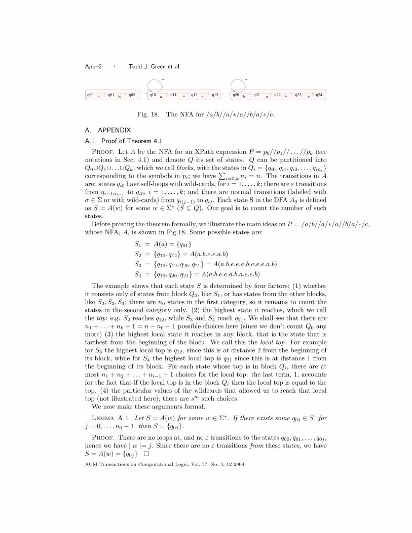
App–2 · Todd J. Green et al.
a b a a b * c* a
* *
q00 q01 q02 q10 q11 q12 q13 q20 q21 q22 q23 q24
Fig. 18. The NFA for /a/b//a/∗/a//b/a/∗/c.
A. APPENDIX
A.1 Proof of Theorem 4.1
Proof. Let A be the NFA for an XPath expression P = p0//p1// . . . //pk (seenotations in Sec. 4.1) and denote Q its set of states. Q can be partitioned intoQ0∪Q1∪. . .∪Qk, which we call blocks, with the states in Qi = {qi0, qi1, qi2, . . . , qini}corresponding to the symbols in pi; we have
∑i=0,k ni = n. The transitions in A
are: states qi0 have self-loops with wild-cards, for i = 1, . . . , k; there are ε transitionsfrom qi−1ni−1 to qi0, i = 1, . . . , k; and there are normal transitions (labeled withσ ∈ Σ or with wild-cards) from qi(j−1) to qij . Each state S in the DFA A0 is definedas S = A(w) for some w ∈ Σ∗ (S ⊆ Q). Our goal is to count the number of suchstates.
Before proving the theorem formally, we illustrate the main ideas on P = /a/b//a/∗/a//b/a/∗/c,whose NFA, A, is shown in Fig.18. Some possible states are:
S1 = A(a) = {q01}S2 = {q10, q12} = A(a.b.e.e.a.b)S3 = {q10, q12, q20, q21} = A(a.b.e.e.a.b.a.e.e.a.b)S4 = {q10, q20, q21} = A(a.b.e.e.a.b.a.e.e.b)
The example shows that each state S is determined by four factors: (1) whetherit consists only of states from block Q0, like S1, or has states from the other blocks,like S2, S3, S4; there are n0 states in the first category, so it remains to count thestates in the second category only. (2) the highest state it reaches, which we callthe top: e.g. S2 reaches q12, while S3 and S4 reach q21. We shall see that there aren1 + . . . + nk + 1 = n− n0 + 1 possible choices here (since we don’t count Q0 anymore) (3) the highest local state it reaches in any block, that is the state that isfarthest from the beginning of the block. We call this the local top. For examplefor S3 the highest local top is q12, since this is at distance 2 from the beginning ofits block, while for S4 the highest local top is q21 since this is at distance 1 fromthe beginning of its block. For each state whose top is in block Qi, there are atmost n1 + n2 + . . . + ni−1 + 1 choices for the local top: the last term, 1, accountsfor the fact that if the local top is in the block Qi then the local top is equal to thetop. (4) the particular values of the wildcards that allowed us to reach that localtop (not illustrated here); there are sm such choices.
We now make these arguments formal.
Lemma A.1. Let S = A(w) for some w ∈ Σ∗. If there exists some q0j ∈ S, forj = 0, . . . , n0 − 1, then S = {q0j}.
Proof. There are no loops at, and no ε transitions to the states q00, q01, . . . , q0j ,hence we have | w |= j. Since there are no ε transitions from these states, we haveS = A(w) = {q0j}ACM Transactions on Computational Logic, Vol. ??, No. 4, 12 2004.
Processing XML Streams with Deterministic Automata and Stream Indexes · App–3
This enables us to separate the sets S = A(w) into two categories: those thatcontain some q0j , j < n0, and those that don’t. Notice that the state q0n0 does notoccur in any set of the first category, and occurs in exactly one set of the secondcategory, namely {q0n0 , q10}, if k > 0 (because of the ε transition between them),and {q0n0}, if k = 0 respectively. There are exactly n0 = prefix(P ) sets S in thefirst category. It remains to count the sets in the second category, and we will showthat there are at most (k2−1
2k2 (n− n0)2 + (n− n0) + (n− n0 − nk) + 1)sm such sets,when k > 0, and exactly one when k = 0: hence, the number of sets of the secondcategory is body(P ), and the total number of states is ≤ prefix(P ) + body(P ). Wewill consider only sets S of the second kind from now on. When k = 0, then theonly such set is {q0n0}, hence we will only consider the case k > 0 in the sequel.
Lemma A.2. Let S = A(w). If qde ∈ S for some d > 0, then for every i =1, . . . , d we have qi0 ∈ S.
Proof. This follows from the fact that the automaton A is linear, hence in orderto reach the state qde the computation for w must go through the state qi0, andfrom the fact that qi0 has a self loop with a wild card.
Lemma A.3. Let S = A(w) and qde ∈ S for some d > 0. Let qij be a statebefore qde, i.e. i < d or i = d and j ≤ e. Then, if we split w into w1.w2 where thelength of w2 is ≤ j, then qi0 ∈ A(w1).
Proof. If the computation for w reaches qde, then it must go through qi0, qi1, . . . , qij .Hence, if we delete j or fewer symbols from the end of w and call the remainingsequence w1 then the computation for w1 will still reach qi0, hence qi0 ∈ A(w1)because of the selfloop at qt0.
We can finally count the maximum number of states S = A(w). We fix a wfor each such S (choosing one nondeterministically) and further associate to S thefollowing triple (qde, qtr, v): qde is the top, i.e. the highest state in S (defined by:∀qij ∈ S, either i < d or i = d and j ≤ e); qtr ∈ S is the local top, i.e. the statewith the largest r (defined formally by ∀qij ∈ S, either j < r or j = r and i ≤ t;that is, in the case of a tie we choose the largest t); finally v is the sequence of thelast r symbols in w. We claim that the triple (qde, qtr, v) uniquely determines S.
First we show that this claim proves the upper bound on the number of setsof the second category, hence proves the theorem. Indeed there are n1 + . . . +nk + 1 = n − n0 + 1 choices for qde. This is because in each block i we canchoose qi0, qi1, . . . , qini−1 as top state: we cannot choose qini
as top state since thisautomatically makes q(i+1)0 the top state, except when i = k then the top statemay be qknk
(and this accounts for the ending +1). For each top state qde there are≤ n1 +n2 + . . .+nd−1 +1 choices for the local top. This is because if we choose thelocal top in some block j with j < d then there are ≤ nj choices14; but if we choosethe local top in the same block d as the global top, then there is a single choice,namely qde, and this accounts for the ending +1. The total number of choices for
14There are exactly nj − e choices when nj > e, and 0 choices when nj ≤ e.
ACM Transactions on Computational Logic, Vol. ??, No. 4, 12 2004.

App–4 · Todd J. Green et al.
(qde, qtr) is bounded by:∑1≤j<i≤k
njni +k∑1
ni︸ ︷︷ ︸when qde 6= qknk
+k−1∑1
ni + 1︸ ︷︷ ︸when qde = qknk
=
=(∑k
1 ni)2 −∑k
1 n2i
2+
k∑1
ni +k−1∑1
ni + 1
≤ 12((
∑ni)2 −
1k2
(∑
ni)2) +k∑1
ni +k−1∑1
ni + 1
=k2 − 12k2
(n− n0)2 + (n− n0) + (n− n0 − nk) + 1
Here we used the inequality:
(k∑
i=1
ni)2 ≤ k2k∑
i=1
n2i
Finally, there are at most sm choices for v since these correspond to choosingsymbols for the wild cards on the path from qt1 to qtr. The total is ≤ (k2−1
2k2 (n −n0)2 + (n− n0) + (n− n0 − nk) + 1)sm, which, as we argued, suffices to prove thetheorem.
It remains to show that the triple (qde, qtr, v) uniquely determines S. Con-sider two states, S, S′, resulting in the same triples (qde, qtr, v). We have S =A(w.v), S′ = A(w′.v) for some sequences u, u′. It suffices to prove that S ⊆ S′ (theinclusion S′ ⊆ S is shown similarly). Let qij ∈ S. Clearly qij is before qde, andj ≤ r. Take out the last j symbols from v: this is possible since the length of vis r, hence v can be written as v = v1.v2, with the lenght of v2 equal to j. Sinceqij is before qde and qde ∈ A(w′.v), by Lemma A.3 we also have qi0 ∈ A(w′.v1).The path from state qi0 to state qij accepts the word v2 because qij ∈ A(w.v1.v2).Hence, qij ∈ A(w′.v1.v2) = S′.
A.2 Proof of Theorem 4.4
Proof. Given a set of XPath expressions Q, one can construct its DFA, A, asfollows. First, for each P ∈ Q, construct the DFA AP . Then, A is given by theproduct automaton
∏P∈Q AQ. From the proof of Theorem 4.1 we know that the
states of AP form two classes: a prefix, which is a linear chain of states, with exactlyprefix(P ) states, followed by a more complex structure with body(P ) states. In theproduct automaton each state in the prefix of some AP occurs exactly once: theseaccount for
∑P∈Q prefix(P ) states in A. The remaining states in A consists of sets
of states, with at most one state from each AP : there are at most∏
P∈Q(1+body(P ))such states.
A.3 Proof of Theorem 4.5
Proof. We introduce some definitions. Let S be a graph schema with symbolsfrom Σ and r its root node. A path is a sequence of nodes, p = (x0, x1, . . . , xn),ACM Transactions on Computational Logic, Vol. ??, No. 4, 12 2004.
Processing XML Streams with Deterministic Automata and Stream Indexes · App–5
n ≥ 0. Every path consists of at least one node, and we denote last(p) = xn itslast node. A rooted path is one that starts at the root, i.e. x0 = r. We denote withL(p) ∈ Σ∗ the sequence of labels on p and L(S) = {L(p) | p rooted path in S}.
To prove the theorem we will replace S with a graph Su obtained by unfoldingS s.t. L(S) = L(Su). In the traditional definition of unfolding the nodes of theunfolded graph are all the rooted path in S, while an edge connects tow paths p,p′ when p′ extends p with one more node. Under this definition, the unfolding is atree, which is infinite in general. We will modify the definition to ensure that theunfolding is finite. Intuitively, we will unfold S in the traditional way, expanding allpossible paths, but checking along each branch that we don’t have repeated nodes.When we are about to repeat a node along a branch, we stop the unfolding andconstruct an edge back to that node on the branch.
Formally, call a path simple if all nodes are distinct. We define the unfoldingof S to be the graph Su whose nodes are all the rooted simple paths in S andwhose edges (p, p′) are of two kinds. Forward edges: p′ extends p with anothernode. Backwards edges: p′ is a prefix of p and there exists an edge from last(p)to last(p′) in S. Clearly the forward edges form a tree, while the backwards edgesintroduce cycles. Finally, Su is labeled as follows: the label of a node p in Su is thesame as the label of last(p) in S.
Recall that a graph schema is simple if any two simple cycles either have disjointsets of nodes or are identical.
Example A.4 We will illustrate some of the concepts in the proof with the fol-lowing example. Consider the following schema S:
Nodes(S):. 1, 2, 3, 4, 5, 6, 7, labels a, b, c, d, e, f, g (i.e. node 1 is labeled a, etc).Edges(S):.
1 → 2 → 3 → 4 → 5 → 6 → 54 → 2
1 → 3 → 7
There are two simple cycles, (2, 3, 4) and (5, 6), and since they are disjoint theschema is ’simple’. The unfolding is:
Nodes(Su):. all simple paths, e.g. 1, 12, 123, 1234, 1237, etc. The label of 12 isb, the label of 123 is c, etc.
Edges(Su). The forward edges, which form a tree, are marked →; Backwardsedges are marked ⇒:
1 → 12 → 123 → 1234 → 12345 → 123456 ⇒ 123451234 ⇒ 12
123 → 12371 → 13 → 134 → 1345 → 13456 ⇒ 1345
134 → 1342 ⇒ 1313 → 137
ACM Transactions on Computational Logic, Vol. ??, No. 4, 12 2004.
App–6 · Todd J. Green et al.
In the following lemmas we fix S a simple graph schema and p = (x0, . . . , xn) arooted simple path.
Lemma A.5. Let C be a simple cycle s.t. C ∩ p 6= ∅. Then there exists i ≤ j s.t.C ∩ p = {xi, xi+1, . . . , xj}; we call this set an interval and denote it [i, j].
Proof. Let xi be the first and xj the last node in C ∩ p, and suppose C ∩ p hasa gap, i.e. xk, xl ∈ C ∩ p but xk+1, xk+2, . . . , xl−1 6∈ C. Let p′ be the set of nodesfrom xk to xl on the cycle C. Define C ′ = (C − p′)∪{xk, xk+1, . . . , xl}. Clearly C ′
is also a simple cycle different from C, and we have C ∩ C ′ 6= ∅, contradicting thefact that S is simple.
Lemma A.6. Let C,C ′ be two different simple cycles s.t. C∩p 6= ∅ and C ′∩p 6=∅. Let [i, j] and [i′, j′] be the intervals as defined in Lemma A.5. Then the intervals[i, j] and [i′, j′] are disjoint.
Proof. Follows immediately from the fact that C and C ′ are disjoint.
Lemma A.7. Let d be the number of simple cycles that p intersects, and denotethese cycles C1, . . . , Cd. Denote with L(p) ⊆ Σ∗ the set of all sequences of labelson all paths in Su from the root to p. Then there exists words w0, w1, . . . , wd ∈ Σ∗
and z1, . . . , zd ∈ Σ+ s.t. L(p) = w0.z∗1 .w1 . . . wd−1.z
∗d .wd.
Example A.8 Before giving the proof, we illustrate the lemma on our runningexample:
L(1234) = a(bcd)∗bcdL(12345) = a(bcd)∗bcd(ef)∗eL(137) = acg
L(1237) = a(bcd)∗bcgL(1342) = a(cdb)∗cdb
Proof. Let [i1, j1], . . . , [id, jd] be the disjoint intervals obtained by intersectingp with C1, . . . , Cd, i.e. p has the form:
p = (. . . , xi1 , . . . , xj1 , . . . , xi2 , . . . , xj2 , . . . , xid, . . . , xjd
, . . .)
and each Ck intersects p precisely at xik, xik+1, . . . , xjk
. Consider any path p0, p1, . . . , pm
in the unfolded schema Su from the root to p, where each pq is a simple path in S,q = 0, . . . ,m. Call pq good if it is either a of the form (x0, . . . , xk (i.e. a prefix ofp), or it is of the form (x0, . . . , xjk
, y1, . . . , yl), where y1, . . . , yl ∈ Ck (i.e. a prefixof p followed by some fragment of Ck). We claim that for each q, pq is good. Inparticular last(pq) is a node belonging either to p or to some cycle Ck. If this claimholds, then it suffices to pick each wk to be the word between xik
and xik+1 (withxi0 defined to be x0 and xid+1 defined to be last(p)), and to pick zk to be the wordon the cycle Ck when traversed starting at the node xik
and it follows that the pathp0, p1, . . . , pm spells out a word in the language w0.z
∗1 .w1 . . . wd−1.z
∗d .wd.
ACM Transactions on Computational Logic, Vol. ??, No. 4, 12 2004.
Processing XML Streams with Deterministic Automata and Stream Indexes · App–7
To prove the claim let q be the largest index for which pq is not good. Then pq+1
is good, hence it is a prefix of pq (because, if pq were a prefix of pq+1, then pq werealso good). Hence there is a cycle C ′ in S going from last(pq+1) to last(pq) andwith one edge back to last(pq+1). This cycle is not one of C1, . . . , Cp (otherwise pq
were the concatenation of pq+1, which is good, and a cycle Ck, and then pq werealso good). We have already established that last(pq+1) belongs to this cycle. Onthe other hand, since pq+1 is good, the node last(qq+1) belongs either to p or toone of the cycles C1, . . . , Cp. The first case however contradicts the fact that p onlyintersects the cycles C1, . . . , Cp, not C ′; the second case contradicts the fact thattwo distinct cycles are disjoint.
Finally, let L(S) be the regular set of all labels on all rooted path in a graphschema S: we have denoted this Lschema in Sec. 4.2.1. Then:
Lemma A.9. If S is a simple graph schema then L(S) = L(Su).
Proof. Obviously L(Su) ⊆ L(S). For the converse, let p = (x0, x1, . . . , xn)be a rooted path in S, and let C1, . . . , Cd be all the simple cycles that it in-tersects. Reasoning as in the proof of Lemma A.7, p can be decomposed intop = p0C
m11 p1C
m22 p2 . . . Cmd
d pd, for some numbers m1, . . . ,md > 0. A similar samepath exists then in Su, hence the word spelled by p is in L(Su).
We now return to the proof of Theorem 4.5. We consider a graph schema S and,by using Lemma A.9 we can assume that S is already unfolded, and that Lemma A.7holds. Then the set of all root-to-leaf sequences allowed by S, L(S) ⊆ Σ∗, can beexpressed as:
L(S) = {ε} ∪⋃
x∈nodes
L(x)
where L(x) denotes all sequences of tags up to the node x in S. Our goal is tocompute the number of states, as given by Eq.(3), with Ldata replaced by L(S).Since the graph schema is simple and each simple path intersects at most d cycles,we have by Lemma A.7:
L(x) = {w0.zm11 .w1 . . . zmd
d .wd |m1 ≥ 1, . . . ,md ≥ 1} (5)
where w0, . . . , wd ∈ Σ∗ and z1, . . . , zd ∈ Σ+. (To simplify the notation we assumedthat the path to x intersects exactly d cycles.) We use a pumping lemma to arguethat, if we increase some mi beyond n (the depth of the query set), then no newstates are generated by Eq.(3). Let u.zm.v ∈ L(x) s.t. m > n. We will show thatAn(u.zm.v) = An(u.zn.v). Assume q ∈ An(u.zn.v). Following the transitions inAn determined by the sequence u.zn.v we notice that the word zn must traverse aself-loop in An, because n is the depth; the self-loop, of course, corresponds to a //in one of the XPath expressions. It follows that u.zm.v has the same computationin An: just follow that loop an additional number of times, hence q ∈ An(u.zm.v).Conversely, let q ∈ An(u.zm.v) and consider the transitions in An determined bythe sequence u.zm.v. Let q′ and q′′ be the beginning and end states of the zm
segment. The shortest path from q′ to q′′ in An has at most n Σ ∪ {∗}-transitionsACM Transactions on Computational Logic, Vol. ??, No. 4, 12 2004.
App–8 · Todd J. Green et al.
(since the depth of the XPath expression is ≤ n), and at most n − 1 self-loops.Consider the smallest number p s.t. ∀p1, p ≤ p1 ≤ m there is a computation fromq′ to q′′ accepting the word zp1 . We will prove that p ≤ n. Suppose the contrary,p > n, and consider a computation of zp from q′ to q′′. Then the computation musttraverse at least one loop |z| times or more, where |z| ≥ 1 is the length of the wordz: for if not, then the word spelled out by the computation has at most length(n−1)(|z|−1)+n < (n−1)|z|+1, hence it couldn’t spell out the word zp. Removeexactly |z| consecutive symbols from zp that traverse that self-loop. The remainingword is zp−1 and there exists a computation for it from q′ to q′′, contradicting thefact that p is minimal such. This proves that u.zn.v also has a computation fromthe initial state in An to q. We have thus concluded that An(u.zm.v) = An(u.zn.v).
As a consequence, there are at most (1+n)d sets in {An(w) | w ∈ L(x)} (namelycorresponding to all possible choices of mi = 0, 1, 2, . . . , n, for i = 1, . . . , d in Eq.(5)).It follows that there are at most 1 + D(1 + n)d states in Al.
A.4 Proof of Theorem 4.8
Proof. Each state in Ati can have at most one transition labeled text(Si):
hence, the number of sink states in Ai is at most si. The automaton for Q = Q1 ∪. . .∪Qq is can be described as the cartesian product automaton A = A1× . . .×Aq,assuming each Ai has been extended with the global sink state ∅, as explained inSec. 3.1. The Σs-sink states15 in A will thus consists of the disjoint union of theΣs-sink states from each Ai, because the transitions leading to Σs-sink states in Ai
and Aj are incompatible, when i 6= j. Hence, there are∑
i si sink states.
A.5 Other Tools in the XML Toolkit
All the other tools are designed to do a single pass over the XML data; we illustratethem here only briefly. Some are straightforward, like xdelete; others are quiteversatile, like xagg, but we omit more interesting examples for lack of space.
A.5.0.9 Aggregation. The xagg command line is given in Fig 15, while somedetails of the -a argument are given in Fig. 19. We illustrate it here with threeexamples:
xagg -c /dblp -a count text *xagg -c /dblp -a count text *
-a count text */author -a avg float */pricexagg -c /dblp/* -a first text title-a count text author -a count text url
The first example counts the total number of publications under dblp. Its resultis:
<xagg><context path="/dblp"><agg type="count" path="*">256599</agg>
</context></xagg>
15We call them that way in order not to confuse them with the ∅ sink state.
ACM Transactions on Computational Logic, Vol. ??, No. 4, 12 2004.
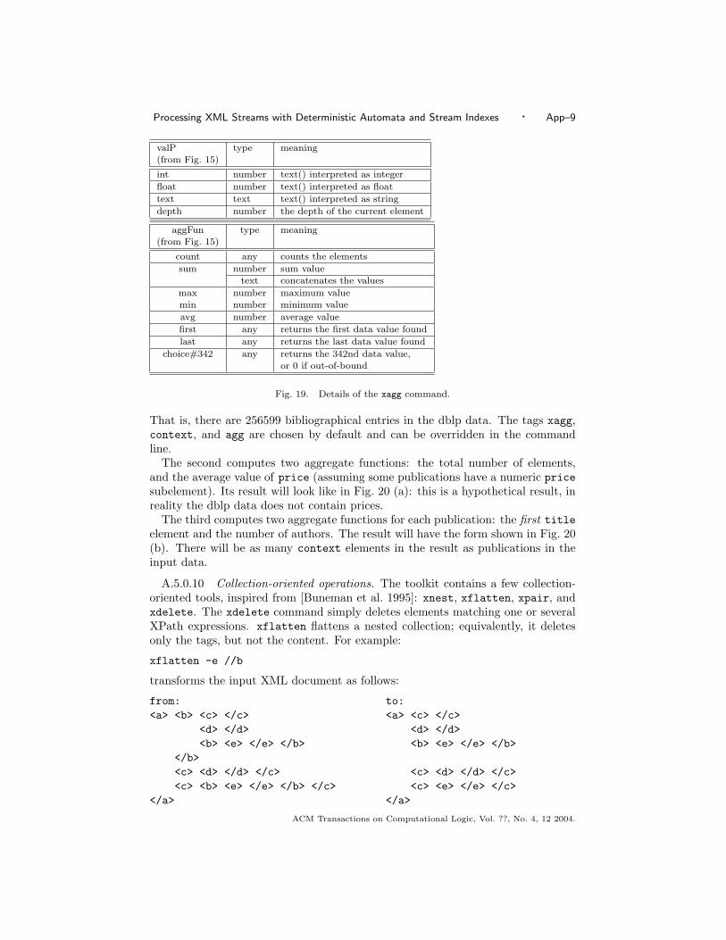
Processing XML Streams with Deterministic Automata and Stream Indexes · App–9
valP type meaning
(from Fig. 15)
int number text() interpreted as integer
float number text() interpreted as float
text text text() interpreted as string
depth number the depth of the current element
aggFun type meaning
(from Fig. 15)
count any counts the elements
sum number sum value
text concatenates the values
max number maximum value
min number minimum value
avg number average value
first any returns the first data value found
last any returns the last data value found
choice#342 any returns the 342nd data value,
or 0 if out-of-bound
Fig. 19. Details of the xagg command.
That is, there are 256599 bibliographical entries in the dblp data. The tags xagg,context, and agg are chosen by default and can be overridden in the commandline.
The second computes two aggregate functions: the total number of elements,and the average value of price (assuming some publications have a numeric pricesubelement). Its result will look like in Fig. 20 (a): this is a hypothetical result, inreality the dblp data does not contain prices.
The third computes two aggregate functions for each publication: the first titleelement and the number of authors. The result will have the form shown in Fig. 20(b). There will be as many context elements in the result as publications in theinput data.
A.5.0.10 Collection-oriented operations. The toolkit contains a few collection-oriented tools, inspired from [Buneman et al. 1995]: xnest, xflatten, xpair, andxdelete. The xdelete command simply deletes elements matching one or severalXPath expressions. xflatten flattens a nested collection; equivalently, it deletesonly the tags, but not the content. For example:
xflatten -e //b
transforms the input XML document as follows:
from: to:<a> <b> <c> </c> <a> <c> </c>
<d> </d> <d> </d><b> <e> </e> </b> <b> <e> </e> </b>
</b><c> <d> </d> </c> <c> <d> </d> </c><c> <b> <e> </e> </b> </c> <c> <e> </e> </c>
</a> </a>
ACM Transactions on Computational Logic, Vol. ??, No. 4, 12 2004.
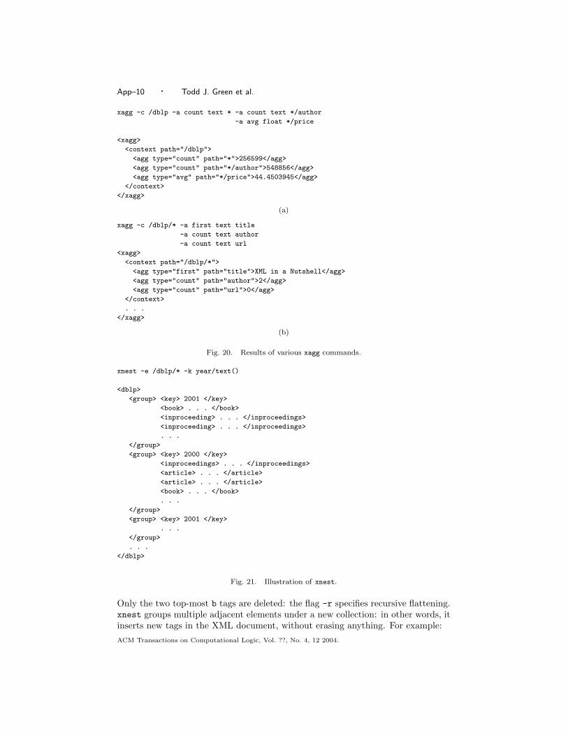
App–10 · Todd J. Green et al.
xagg -c /dblp -a count text * -a count text */author
-a avg float */price
<xagg>
<context path="/dblp">
<agg type="count" path="*">256599</agg>
<agg type="count" path="*/author">548856</agg>
<agg type="avg" path="*/price">44.4503945</agg>
</context>
</xagg>
(a)
xagg -c /dblp/* -a first text title
-a count text author
-a count text url
<xagg>
<context path="/dblp/*">
<agg type="first" path="title">XML in a Nutshell</agg>
<agg type="count" path="author">2</agg>
<agg type="count" path="url">0</agg>
</context>
. . .
</xagg>
(b)
Fig. 20. Results of various xagg commands.
xnest -e /dblp/* -k year/text()
<dblp>
<group> <key> 2001 </key>
<book> . . . </book>
<inproceeding> . . . </inproceedings>
<inproceeding> . . . </inproceedings>
. . .
</group>
<group> <key> 2000 </key>
<inproceedings> . . . </inproceedings>
<article> . . . </article>
<article> . . . </article>
<book> . . . </book>
. . .
</group>
<group> <key> 2001 </key>
. . .
</group>
. . .
</dblp>
Fig. 21. Illustration of xnest.
Only the two top-most b tags are deleted: the flag -r specifies recursive flattening.xnest groups multiple adjacent elements under a new collection: in other words, itinserts new tags in the XML document, without erasing anything. For example:ACM Transactions on Computational Logic, Vol. ??, No. 4, 12 2004.
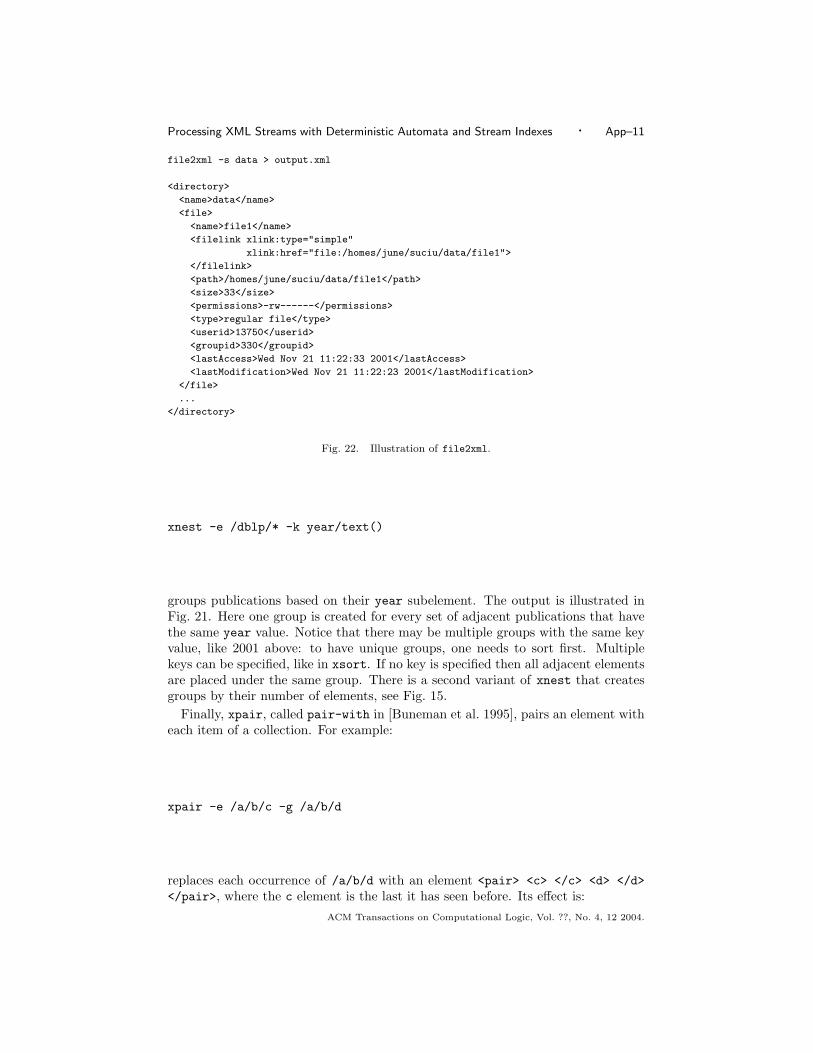
Processing XML Streams with Deterministic Automata and Stream Indexes · App–11
file2xml -s data > output.xml
<directory>
<name>data</name>
<file>
<name>file1</name>
<filelink xlink:type="simple"
xlink:href="file:/homes/june/suciu/data/file1">
</filelink>
<path>/homes/june/suciu/data/file1</path>
<size>33</size>
<permissions>-rw------</permissions>
<type>regular file</type>
<userid>13750</userid>
<groupid>330</groupid>
<lastAccess>Wed Nov 21 11:22:33 2001</lastAccess>
<lastModification>Wed Nov 21 11:22:23 2001</lastModification>
</file>
...
</directory>
Fig. 22. Illustration of file2xml.
xnest -e /dblp/* -k year/text()
groups publications based on their year subelement. The output is illustrated inFig. 21. Here one group is created for every set of adjacent publications that havethe same year value. Notice that there may be multiple groups with the same keyvalue, like 2001 above: to have unique groups, one needs to sort first. Multiplekeys can be specified, like in xsort. If no key is specified then all adjacent elementsare placed under the same group. There is a second variant of xnest that createsgroups by their number of elements, see Fig. 15.
Finally, xpair, called pair-with in [Buneman et al. 1995], pairs an element witheach item of a collection. For example:
xpair -e /a/b/c -g /a/b/d
replaces each occurrence of /a/b/d with an element <pair> <c> </c> <d> </d></pair>, where the c element is the last it has seen before. Its effect is:
ACM Transactions on Computational Logic, Vol. ??, No. 4, 12 2004.
App–12 · Todd J. Green et al.
from<a> <b> <c> 1 </c>
<d> 2 </d><d> 3 </d>
</b><b> <d> 4 </d> </b><b> <c> 5 </c>
<d> 6 </d></b>
</a>
to<a> <b> <c> 1 </c>
<pair> <c> 1 </c><d> 2 </d>
</pair><pair> <c> 1 </c>
<d> 3 </d></pair>
</b><b> <pair> <c> 1 </c>
<d> 4 </d></pair>
</b><b> <c> 5 </c>
<pair> <c> 5 </c><d> 6 </d>
</pair></b>
</a>
A.5.0.11 Heads or Tails?. xhead and xtail select and output the head or tailof a sequence of elements matching one or several XPath expressions. For example:
xhead -c /dblp -e book -n 20 -e article
outputs only the first 20 book elements and the first 10 (default value) articleelements under dblp.
A.5.0.12 File Directories to XML. The file2xml generates an XML file thatdescribes a file directory hierarchy. For example:
file2xml -s data > output.xml
traverses the data directory and all its subdirectories and creates the output.xmldocument which has an isomorphic structure to the directory hierarchy. The outputis shown in Fig. 22.
As another example, the command below lists the top ten largest files in a direc-tory hierarchy:
file2xml -s . | xsort -b -c /directory-e //file -k size/text():%i |xhead -c /directory -e file
The %i option in xsort indicates that size is an integer field.
ACM Transactions on Computational Logic, Vol. ??, No. 4, 12 2004.