16‐731

“Processesofadpatationinfarmdecision‐makingmodels.Areview”

MarionRobert,AlbanThomasandJacques‐EricBergez

November2016

PROCESSES OF ADAPTATION IN FARM DECISION-MAKING 1

MODELS. A REVIEW 2

3

4

Marion Robert1,*, Alban Thomas2, Jacques-Eric Bergez1 5

6

¹ INRA, Université Fédérale de Toulouse, UMR 1248 AGIR, F-31326 Castanet-Tolosan, France 7

² Toulouse School of Economics, INRA, University of Toulouse, F-31000 Toulouse, France 8

9

*: Corresponding author, Tel: +33 (0)5 61 28 50 30. E-mail: marion.robert@toulouse.inra.fr 10

11

12

Forthcoming in Agronomy for Sustainable Development 13

Review Article 14

15

ABSTRACT 16

Agricultural production systems are facing new challenges due to an ever changing global 17

environment that is a source of risk and uncertainty. To adapt to these environmental changes, farmers 18

must adjust their management strategies and remain competitive while also satisfying societal 19

preferences for sustainable food systems. Representing and modeling farmers’ decision-making 20

processes by including adaptation, when representing farmers’ practices ,is therefore an important 21

challenge for the agricultural research community. 22

Bio-economic and bio-decisional approaches have addressed adaptation at different planning horizons 23

in the literature. We reviewed approximately 40 articles using bio-economic and bio-decisional models 24

in which strategic and tactical decisions were considered dynamic adaptive and expectation-based 25

processes. The main results of this literature survey are as follows: i) adaptability, flexibility and 26

dynamic processes are common ways to characterize farmers’ decision-making, ii) adaptation can be a 27

reactive or a proactive process depending on farmers’ flexibility and expectation capabilities, and iii) 28

different modeling approaches are used to model decision stages in time and space, and some 29

approaches can be combined to represent a sequential decision-making process. Focusing attention on 30

short- and long-term adjustments in farming production plans, coupled with sequential and 31

anticipatory approaches should lead to promising improvements for assisting decision makers. 32

33

Keywords: farmers’ decision-making, bio-economic model, bio-decisional model, uncertainty, 34

adaptation 35

Abstract ................................................................................................................................................... 2 36

1.  Introduction ..................................................................................................................................... 4 37

2.  Background on modeling decisions in agricultural economics and agronomy ............................... 6 38

3.  Method ............................................................................................................................................ 8 39

4.  Formalisms to manage adaptive decision-making processes .......................................................... 9 40

4.1.  Formalisms in proactive adaptation processes ........................................................................ 9 41

4.1.1.  Anticipated shocks in sequential decision-making processes ............................................. 9 42

4.1.2.  Flexible plan with optional paths and interchangeable activities ...................................... 10 43

4.1.3.  Relaxed constraints on executing activities ....................................................................... 10 44

4.2.  Formalisms in reactive adaptation processes......................................................................... 10 45

4.2.1.  Gradual adaptation in a repeated process .......................................................................... 10 46

4.2.2.  Adaptation in sequential decision-making processes ........................................................ 11 47

4.2.3.  Reactive plan with revised and new decision rules ........................................................... 12 48

5.  Modeling adaptive decision-making processes in farming systems .............................................. 12 49

5.1.  Adaptations and strategic decisions for the entire farm ........................................................ 12 50

5.2.  Adaptation and tactic decisions ............................................................................................. 13 51

5.2.1.  Adaptation for the agricultural season and the farm .......................................................... 13 52

5.2.2.  Adaptation of daily activities at the plot scale ................................................................... 14 53

5.3.  Sequential adaptation of strategic and tactical decisions ....................................................... 15 54

6.  Discussion ..................................................................................................................................... 16 55

6.1.  Adaptation: reactive or proactive process? ............................................................................ 16 56

6.2.  Decision-making processes: multiple stages and sequential decisions ................................. 17 57

6.3.  What about social sciences? .................................................................................................. 18 58

6.4.  Uncertainty and dynamic properties ...................................................................................... 18 59

7.  Conclusion ..................................................................................................................................... 19 60

Acknowledgements ............................................................................................................................... 19 61

References ............................................................................................................................................. 20 62

Table caption ......................................................................................................................................... 28 63

Figure caption ........................................................................................................................................ 30 64

1. INTRODUCTION 65

Agricultural production systems are facing new challenges due to a constantly changing global 66

environment that is a source of risk and uncertainty, and in which past experience is not sufficient to 67

gauge the odds of a future negative event. Concerning risk, farmers are exposed to production risk 68

mostly due to climate and pest conditions, to market risk that impact input and output prices, and 69

institutional risk through agricultural, environmental and sanitary regulations (Hardaker 2004). 70

Farmers may also face uncertainty due to rare events affecting, e.g., labor, production capital stock, 71

and extreme climatic conditions , which add difficulties to producing agricultural goods and calls for 72

re-evaluating current production practices. To remain competitive, farmers have no choice but to adapt 73

and adjust their daily management practices (Hémidy et al. 1996; Hardaker 2004; Darnhofer et al. 74

2010; Dury 2011). In the early 1980s, Petit developed the theory of the “farmer’s adaptive behavior” 75

and claimed that farmers have a permanent capacity for adaptation (Petit 1978). Adaptation refers to 76

adjustments in agricultural systems in response to actual or expected stimuli through changes in 77

practices, processes and structures and their effects or impacts on moderating potential modifications 78

and benefiting from new opportunities (Grothmann and Patt 2003; Smit and Wandel 2006). Another 79

important concept in the scientific literature on adaptation is the concept of adaptive capacity or 80

capability (Darnhofer 2014). This refers to the capacity of the system to resist evolving hazards and 81

stresses (Ingrand et al. 2009; Dedieu and Ingrand 2010) and it is the degree to which the system can 82

adjust its practices, processes and structures to moderate or offset damages created by a given change 83

in its environment (Brooks and Adger 2005; Martin 2015). For authors in the early 1980s such as Petit 84

(1978) and Lev and Campbell (1987), adaptation is seen as the capacity to challenge a set of 85

systematic and permanent disturbances. Moreover, agents integrate long-term considerations when 86

dealing with short term changes in production. Both claims lead to the notion of a permanent need to 87

keep adaptation capability under uncertainty. Holling (2001) proposed a general framework to 88

represent the dynamics of a socio-ecological system based on both ideas above, in which dynamics are 89

represented as a sequence of “adaptive cycles”, each affected by disturbances. Depending on whether 90

the latter are moderate or not, farmers may have to reconfigure the system, but if such redesigning 91

fails, then the production system collapses. 92

Some of the most common dimensions in adaptation research on individual behavior refer to the 93

timing and the temporal and spatial scopes of adaptation (Smit et al. 1999; Grothmann and Patt 2003). 94

The first dimension distinguishes proactive vs. reactive adaptation. Proactive adaptation refers to 95

anticipated adjustment, which is the capacity to anticipate a shock (change that can disturb farmers’ 96

decision-making processes); it is also called anticipatory or ex-ante adaptation. Reactive adaptation is 97

associated with adaptation performed after a shock; it is also called responsive or ex-post adaptation 98

(Attonaty et al. 1999; Brooks and Adger 2005; Smit and Wandel 2006). The temporal scope 99

distinguishes strategic adaptations from tactical adaptations, the former referring to the capacity to 100

adapt in the long term (years), while the latter are mainly instantaneous short-term adjustments 101

(seasonal to daily) (Risbey et al. 1999; Le Gal et al. 2011). The spatial scope of adaptation opposes 102

localized adaptation versus widespread adaptation. In a farm production context, localized adaptations 103

are often at the plot scale, while widespread adaptation concerns the entire farm. Temporal and spatial 104

scopes of adaptation are easily considered in farmers’ decision-making processes; however, 105

incorporating the timing scope of farmers’ adaptive behavior is a growing challenge when designing 106

farming systems. 107

System modeling and simulation are interesting approaches to designing farming systems which allow 108

limiting the time and cost constraints (Rossing et al. 1997; Romera et al. 2004; Bergez et al. 2010) 109

encountered in other approaches, such as diagnosis (Doré et al. 1997), systemic experimentation 110

(Mueller et al. 2002) and prototyping (Vereijken 1997). Modeling adaptation to uncertainty, when 111

representing farmers’ practices and decision-making processes, has been addressed in bio-economic 112

and bio-decisional approaches (or management models) and addressed at different temporal and 113

spatial scales. 114

The aim of this paper is to review the way adaptive behavior in farming systems has been considered 115

(modeled)in bio-economic and bio-decisional approaches. This work reviews several modeling 116

formalisms that have been used in bio-economic and bio-decisional approaches, comparing their 117

features and selected relevant applications. We chose to focus on the formalisms rather than the tools 118

as they are the essence of the modeling approach. 119

Approximately 40 scientific references on this topic were found in the agricultural economics and 120

agronomy literature. This paper reviews approaches used to model farmers’ adaptive behavior when 121

they encounter uncertainty in specific stages of, or throughout, the decision-making process. There is a 122

vast literature on technology adoption in agriculture, which can be considered a form of adaptation, 123

but which we do not consider here, to focus on farmer decisions for a given production technology. 124

After presenting some background on modeling decisions in agricultural economics and agronomy and 125

the methodology used, we present formalisms describing proactive behavior and anticipation decision-126

making processes and formalisms for representing reactive adaptation decision-making processes. 127

Then, we illustrate the use of such formalisms in papers on modeling farmers’ decision-making 128

processes in farming systems. Finally, we discuss the need to include adaptation and anticipation to 129

uncertain events in modeling approaches of the decision-making process and discuss adaptive 130

processes in other domains. 131

2. BACKGROUND ON MODELING DECISIONS IN AGRICULTURAL ECONOMICS AND 132

AGRONOMY 133

Two main fields dominate decision-making approaches in farm management: agricultural economics 134

(with bio-economic models) and agronomy (with bio-decisional models). Agricultural economists are 135

typically interested in the analysis of year-to-year strategical (sometimes tactical) decisions originating 136

from long-term strategies (e.g., investment and technical orientation). In contrast, agronomists focus 137

more on day-to-day farm management described in tactical decisions. The differences in temporal 138

scale are due to the specific objective of each approach. For economists, the objective is to efficiently 139

use scarce resources by optimizing the configuration and allocation of farm resources given farmers’ 140

objectives and constraints in a certain production context. For agronomists, it is to organize farm 141

practices to ensure farm production from a bio-physical context (Martin et al. 2013). Agronomists 142

identify relevant activities for a given production objective, their interdependency, what preconditions 143

are needed to execute them and how they should be organized in time and space. Both bio-economic 144

and bio-decisional models represent farmers’ adaptive behavior. 145

146

Bio-economic models integrate both biophysical and economic components (Knowler 2002; Flichman 147

2011). In this approach, equations describing a farmer’s resource-management decisions are combined 148

with those representing inputs to and outputs from agricultural activities (Janssen and van Ittersum 149

2007). The main goal of farm-resource allocation in time and space is to improve economic 150

performance of farming systems, usually along with environmental performance. Bio-economic 151

models indicate the optimal management behavior to adopt by describing agricultural activities. 152

Agricultural activities are characterized by an enterprise and a production technology used to manage 153

the activity. Technical coefficients represent relations between inputs and outputs by stating the 154

amount of inputs needed to achieve a certain amount of outputs (e.g., matrix of input-output 155

coefficients, see Janssen and van Ittersum 2007). Many farm-management decisions can be formulated 156

as a multistage decision-making process in which farmer decision-making is characterized by a 157

sequence of decisions made to meet farmer objectives. The time periods that divide the decision-158

making process are called stages and represent the moments when decisions must be made. Decision 159

making is thus represented as a dynamic and sustained process in time (Bellman 1954; Mjelde 1986; 160

Osman 2010). This means that at each stage, technical coefficients are updated to proceed to the next 161

round of optimization. Three major mathematical programming techniques are commonly used to 162

analyze and solve models of decision under uncertainty: recursive models, dynamic stochastic 163

programming, and dynamic programming (see Miranda and Fackler 2004). Agricultural economic 164

approaches usually assume an idealized situation for decision, in which the farmer has clearly 165

expressed goals from the beginning and knows all the relevant alternatives and their consequences. 166

Since the farmer’s rationality is considered to be complete, it is feasible to use the paradigm of utility 167

maximization (Chavas et al. 2010). Simon (1950) criticized this assumption of full rationality and 168

claimed that decision-makers do not look for the best decision but for a satisfying one given the 169

amount of information available. This gave rise to the concept of bounded and adaptive rationality 170

(Simon 1950; Cyert and March 1963), in which the rationality of decision-makers is limited by the 171

information available, cognitive limitations of their minds and the finite timing of the decision. In 172

bounded rationality, farmers tend to seek satisfactory rather than utility maximization when making 173

relevant decisions (Kulik and Baker, 2008). From complete or bounded rationality, all bio-economic 174

approaches are characterized by the common feature of computing a certain utility value for available 175

options and then selecting the one with the best or satisfactory value. In applied agricultural 176

economics, stochastic production models are more and more commonly used to represent the 177

sequential production decisions by farmers, by specifying the production technology through a series 178

of operational steps involving production inputs. These inputs have often the dual purpose of 179

controlling crop yield or cattle output level on the one hand, and controlling production risk on the 180

other (Burt 1993; Maatman et al. 2002; Ritten et al. 2010). Furthermore, sequential production 181

decisions with risk and uncertainty can also be specified in a dynamic framework, to account for 182

intertemporal substitutability between inputs (Fafchamps 1993). Dynamic programming models have 183

been used as guidance tools in policy analysis and to help farmers identify irrigation strategies (Bryant 184

et al. 1993). 185

Biophysical models have been investigated since the 1970s, but the difficulty in transferring 186

simulation results to farmers and extension agents led researchers to investigate farmers’ management 187

practices closely and develop decision models (Bergez et al. 2010). A decision model, also known as a 188

decision-making process model or farm-management model, comes from on-farm observations and 189

extensive studies of farmers’ management practices. These studies, which show that farmers’ technical 190

decisions are planned, led to the “model for action” concept (Matthews et al. 2002), in which decision-191

making processes are represented as a sequence of technical acts. Rules that describe these technical 192

acts are organized in a decision schedule that considers sequential, iterative and adaptive processes of 193

decisions (Aubry et al. 1998). In the 1990s, combined approaches represented farming systems as bio-194

decisional models that link the biophysical component to a decisional component based on a set of 195

decision rules (Aubry et al. 1998; Attonaty et al. 1999; Bergez et al. 2006; Bergez et al. 2010). Bio-196

decisional models describe the appropriate farm-management practice to adopt as a set of decision 197

rules that drives the farmer’s actions over time (e.g., a vector returning a value for each time step of 198

the simulation). Bio-decisional models are designed (proactive) adaptations to possible but anticipated 199

changes. By reviewing the decision rules, these models also describe the farmer’s reactive behavior. 200

3. METHOD 201

To achieve the above goal, a collection of articles was assembled through three steps. The first step 202

was a search on Google Scholar using the following combination of Keywords: Topic = ((decision-203

making processes) or (decision model) or (knowledge-based model) or (object-oriented model) or 204

(operational model)) AND Topic = ((bio-economics or agricultural economics) or (agronomy or bio-205

decisional)) AND Topic = ((adaptation) or (uncertainty) or (risk)). The first topic defines the tool of 206

interest: only work using decision-making modeling (as this is the focus of this paper). Given that 207

different authors use slightly different phrasings, the present paper incorporated the most-commonly 208

used alternative terms such as knowledge-based model, object-oriented model, and operational model. 209

The second topic restricts the search to be within the domains of bio-economics and agronomy. The 210

third topic reflects the major interest of this paper, which relates to farmer adaptations facing uncertain 211

events. This paper did not use “AND” to connect the parts within topics because this is too restrictive 212

and many relevant papers are filtered out. 213

The second step was a classification of formalisms referring to the timing scopes of the adaptation. We 214

retained the timing dimension as the main criteria for the results description in our paper. The timing 215

dimension is an interesting aspect of adaptation to consider when modeling adaptation in farmers’ 216

decision-making processes. Proactive processes concern the ability to anticipate future and external 217

shocks affecting farming outcomes and to plan corresponding adjustments. In this case, adaptations 218

processes are time-invariant and formalisms describing static processes are the most appropriate since 219

they describe processes that do not depend explicitly on time. Reactive processes describe the farmer’s 220

capacity to react to a shock. In this case, adaptation concerns the ability to update the representation of 221

a shock and perform adaptations without any anticipation. In this case adaptation processes are time-222

dependent and formalisms describing dynamic processes are the most appropriate since they describe 223

processes that depend explicitly on time (Figure 1). Section 4 will present the results of running this 224

step. 225

The third step was a classification of articles related to farm management in agricultural economics 226

and agronomy referring to the temporal and spatial scopes of the adaptation. This last step aimed at 227

illustrating the use of the different formalisms presented in the second step to model adaptation within 228

farmer decision-making processes. This section is not supposed to be exhaustive but to provide 229

examples of use in farming system literature. Section 5 will be presenting the results of running this 230

step. 231

4. FORMALISMS TO MANAGE ADAPTIVE DECISION-MAKING PROCESSES 232

This section aims at listing formalisms used to manage adaptive decision-making processes in both 233

bio-economic and bio-decision models. Various formalisms are available to describe adaptive 234

decision-making processes. Adaptation processes can be time-invariant when it is planned beforehand 235

with a decision tree, alternative and optional paths and relaxed constraints to decision processes. 236

Adaptation processes can be time-varying when it is reactive to a shock with dynamic internal changes 237

of the decision process via recursive decision, sequential decision or reviewed rules. We distinguish 238

proactive or anticipated processes to reactive processes. Six formalisms were included in this review. 239

4.1. Formalisms in proactive adaptation processes 240

In proactive or anticipated decision processes, adaptation consists in the iterative interpretation of a 241

flexible plan built beforehand. The flexibility of this anticipatory specification that allows for 242

adaptation is obtained by the ability to use alternative paths, optional paths or by relaxing constraints 243

that condition a decision. 244

4.1.1. Anticipated shocks in sequential decision-making processes 245

When decision-making process is assumed to be a succession of decisions to make, it follows that 246

farmers are able to integrate new information about the environment at each stage and adapt to 247

possible changes occurring between two stages. Farmers are able to anticipate all possible states of the 248

shock (change) to which they will have to react. In 1968, Cocks stated that discrete stochastic 249

programming (DSP) could provide solutions to sequential decision problems (Cocks 1968). DSP 250

processes sequential decision-making problems in discrete time within a finite time horizon in which 251

knowledge about random events changes over time (Rae 1971; Apland and Hauer 1993). During each 252

stage, decisions are made to address risks. One refers to “embedded risk” when decisions can be 253

divided between those initially made and those made at a later stage, once an uncertain event has 254

occurred (Trebeck and Hardaker 1972; Hardaker 2004). The sequential and stochastic framework of 255

the DSP can be represented as a decision tree in which nodes describe the decision stages and branches 256

describe anticipated shocks. Considering two stages of decision, the decision-maker makes an initial 257

decision ( ) with uncertain knowledge of the future. After one of the states of nature of the uncertain 258

event occurs (k), the decision-maker will adjust by making another decision ( ) in the second stage, 259

which depends on the initial decision and the state of nature k of the event. Models can become 260

extremely large when numerous states of nature are considered; this “curse of dimensionality” is the 261

main limitation of these models (Trebeck and Hardaker 1972; Hardaker 2004). 262

4.1.2. Flexible plan with optional paths and interchangeable activities 263

In manufacturing, proactive scheduling is well-suited to build protection against uncertain events into 264

a baseline schedule (Herroelen and Leus 2004; Darnhofer and Bellon 2008). Alternative paths are 265

considered and choices are made at the operational level while executing the plan. This type of 266

structure has been used in agriculture as well, with flexible plans that enable decision-makers to 267

anticipate shocks. Considering possible shocks that may occur, substitutable components, 268

interchangeable partial plans, and optional executions are identified and introduced into the nominal 269

plan. Depending on the context, a decision is made to perform an optional activity or to select an 270

alternative activity or partial plan (Martin-Clouaire and Rellier 2009). Thus, two different sequences of 271

events would most likely lead to performing two different plans. Some activities may be cancelled in 272

one case but not in the other depending on whether they are optional or subject to a context-dependent 273

choice (Bralts et al. 1993; Castellazzi et al. 2008; Dury et al. 2010; Castellazzi et al. 2010). 274

4.1.3. Relaxed constraints on executing activities 275

Management operations on biophysical entities are characterized by a timing of actions depending on 276

their current states. The concept of bounded rationality, presented earlier, highlights the need to obtain 277

satisfactory results instead of optimal ones. Following the same idea, Kemp and Michalk (2007) point 278

out that “farmers can manage more successfully over a range than continually chasing optimum or 279

maximum values”. In practice, one can easily identify an ideal time window in which to execute an 280

activity that is preferable or desirable based on production objectives instead of setting a specific 281

execution date in advance (Shaffer and Brodahl 1998a; Aubry et al. 1998; Taillandier et al. 2012). 282

Timing flexibility helps in managing uncontrollable factors. 283

4.2. Formalisms in reactive adaptation processes 284

In reactive decision processes, adaptation consists in the ability to perform decisions without any 285

anticipation by integrating gradually new information. Reactivity is obtained by multi-stage and 286

sequential decision processes and the integration of new information or the set-up of unanticipated 287

path within forehand plan. 288

4.2.1. Gradual adaptation in a repeated process 289

The recursive method was originally developed by Day (1961) to describe gradual adaptation to 290

changes in exogenous parameters after observing an adjustment between a real situation and an 291

optimal situation obtained after optimization (Blanco-Fonseca et al. 2011). Recursive models 292

explicitly represent multiple decision stages and optimize each one; the outcome of stage n is used to 293

reinitialize the parameters of stage n+1. These models consist of a sequence of mathematical 294

programming problems in which each sub-problem depends on the results of the previous sub-295

problems (Day 1961; Day 2005; Janssen and van Ittersum 2007; Blanco-Fonseca et al. 2011). In each 296

sub-problem, dynamic variables are re-initialized and take the optimal values obtained in the previous 297

sub-problem. Exogenous changes (e.g., rainfall, market prices) are updated at each optimization step. 298

For instance, the endogenous feedback mechanism for a resource (e.g., production input or natural 299

resource) between sub-periods is represented with a first-order linear difference equation: = 300

G ∗ + Y + ,where the resource level of period t ( ) depends on the optimal decisions 301

( ∗ and resource level at t-1 ( and on exogenous variables ( . The Bayesian approach is the 302

most natural one for updating parameters in a dynamic system, given incoming period-dependent 303

information. Starting with an initial prior probability for the statistical distribution of model 304

parameters, sample information is used to update the latter in an efficient and fairly general way 305

(Stengel 1986). The Bayesian approach to learning in dynamic systems is a special but important case 306

of closed-loop models, in which a feedback loop regulates the system as follows: depending on the 307

(intermediate) observed state of the system, the control variable (the input) is automatically adjusted to 308

provide path correction as a function of model performance in the previous period. 309

4.2.2. Adaptation in sequential decision-making processes 310

In the 1950s, Bellman presented the theory of dynamic programming (DP) to emphasize the sequential 311

decision-making approach. Within a given stage, the decision-making process is characterized by a 312

specific status corresponding to the values of state variables. In general, this method aims to transform 313

a complex problem into a sequence of simpler problems whose solutions are optimal and lead to an 314

optimal solution of the initial complex model. It is based on the principle of optimality, in which “an 315

optimal policy has the property that whatever the initial state and decisions are, the remaining 316

decisions must constitute an optimal policy with regard to the state resulting from the first decisions” 317

(Bellman 1954). DP explicitly considers that a decision made in one stage may affect the state of the 318

decision-making process in all subsequent stages. State-transition equations are necessary to link the 319

current stage to its successive or previous stage, depending on whether one uses a forward or 320

backward DP approach, respectively. In the Bellman assumptions (backward DP), recursion occurs 321

from the future to the present, and the past is considered only for the initial condition. In forward DP, 322

stage numbering is consistent with real time. The optimization problem defined at each stage can 323

result in the application of a wide variety of techniques, such as linear programming (Yaron and Dinar 324

1982) and parametric linear programming (Stoecker et al. 1985). Stochastic DP is a direct extension of 325

the framework described above, and efficient numerical techniques are now available to solve such 326

models, even though the curse of dimensionality may remain an issue (Miranda and Fackler 2004). 327

4.2.3. Reactive plan with revised and new decision rules 328

An alternative to optimization is to represent decision-making processes as a sequence of technical 329

operated organized through a set of decision rules. This plan is reactive when rules are revised or 330

newly introduced after a shock. Revision is possible with simulation-based optimization, in which the 331

rule structure is known and the algorithm looks for optimal indicator values or thresholds. It generates 332

a new set of indicator thresholds to test at each new simulation loop (Nguyen et al. 2014). For small 333

discrete domains, the complete enumeration method can be used, whereas when the optimization 334

domain is very large and a complete enumeration search is no longer possible, heuristic search 335

methods are considered, such as local searching and branching methods. Search methods start from a 336

candidate solution and randomly move to a neighboring solution by applying local changes until a 337

solution considered as optimal is found or a time limit has passed. Metaheuristic searches using 338

genetic algorithms, Tabu searches and simulated annealing algorithms are commonly used. Control-339

based optimization is used to add new rules to the plan. In this case, the rule structure is unknown, and 340

the algorithm optimizes the rule’s structure and optimal indicator values or thresholds. Crop-341

management decisions can be modeled as a Markov control problem when the distribution of variable 342

depends only on the current state and on decision that was applied at stage i. The decision-343

making process is divided into a sequence of N decision stages. It is defined by a set of possible states 344

s, a set of possible decisions d, probabilities describing the transitions between successive states and 345

an objective function (sum of expected returns) to be maximized. In a Markov control problem, a 346

trajectory is defined as the result of choosing an initial state s and applying a decision d for each 347

subsequent state. The DSP and DP methods provide optimal solutions for Markov control problems. 348

Control-based optimization and metaheuristic searches are used when the optimization domain is very 349

large and a complete enumeration search is no longer possible. 350

5. MODELING ADAPTIVE DECISION-MAKING PROCESSES IN FARMING SYSTEMS 351

This section aims at illustrating the use of formalisms to manage adaptive decision-making processes 352

in farming systems both in bio-economic and bio-decision models. Around 40 papers using the six 353

formalisms on adaptation have been found. We distinguish strategic adaptation at the farm level, tactic 354

adaptation at the farm and plot scale and strategic and tactic adaptation both at the farm and plot scale. 355

5.1. Adaptations and strategic decisions for the entire farm 356

Strategic decisions aim to build a long-term plan to achieve farmer production goals depending on 357

available resources and farm structure. For instance, this plan can be represented in a model by a 358

cropping plan that selects the crops grown on the entire farm, their surface area and their allocation 359

within the farmland. It also offers long-term production organization, such as considering equipment 360

acquisition and crop rotations. In the long-term, uncertain events such market price changes, climate 361

events and sudden resource restrictions are difficult to predict, and farmers must be reactive and adapt 362

their strategic plans. 363

Barbier and Bergeron (1999) used the recursive process to address price uncertainty in crop and 364

animal production systems; the selling strategy for the herd and cropping pattern were adapted each 365

year to deal with price uncertainty and policy intervention over 20 years. Similarly, Heidhues (1966) 366

used a recursive approach to study the adaptation of investment and sales decisions to changes in crop 367

prices due to policy measures. Domptail and Nuppenau (2010) adjusted, in a recursive process, herd 368

size and the purchase of supplemental fodder once a year, depending on the available biomass that 369

depended directly on rainfall. In a study of a dairy-beef-sheep farm in Northern Ireland, Wallace and 370

Moss (2002) examined the effect of possible breakdowns due to bovine spongiform encephalopathy 371

on animal-sale and machinery-investment decisions over a seven-year period with linear programming 372

and a recursive process. 373

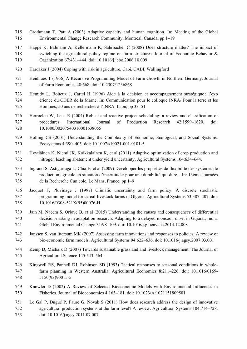
Thus, in the operation research literature, adaptation of a strategic decision is considered a dynamic 374

process that should be modeled via a formalism describing a reactive adaptation processes (Table 1). 375

5.2. Adaptation and tactic decisions 376

5.2.1. Adaptation for the agricultural season and the farm 377

At the seasonal scale, adaptations can include reviewing and adapting the farm’s selling and buying 378

strategy, changing management techniques, reviewing the crop varieties grown to adapt the cropping 379

system and deciding the best response to changes and new information obtained about the production 380

context at the strategic level, such as climate (Table 1). 381

DSP was used to describe farmers’ anticipation and planning of sequential decision stages to adapt to 382

an embedded risk such as rainfall. In a cattle farm decision-making model, Trebeck and Hardaker 383

(1972) represented adjustment in feed, herd size and selling strategy in response to rainfall that 384

impacted pasture production according to a discrete distribution with “good”, “medium”, or “poor” 385

outcomes. After deciding about land allocation, rotation sequence, livestock structure and feed source, 386

Kingwell et al. (1993) considered that wheat-sheep farmers in western Australia have two stages of 387

adjustment to rainfall in spring and summer: reorganizing grazing practices and adjusting animal feed 388

rations. In a two-stage model, Jacquet and Pluvinage (1997) adjusted the fodder or grazing of the herd 389

and quantities of products sold in the summer depending on the rainfall observed in the spring; they 390

also considered reviewing crop purposes and the use of crops as grain to satisfy animal-feed 391

requirements. Ritten et al. (2010) used a dynamic stochastic programming approach to analyze optimal 392

stocking rates facing climate uncertainty for a stocker operation in central Wyoming. The focus was 393

on profit maximization decisions on stocking rate based on an extended approach of predator-prey 394

relationship under climate change scenarios. The results suggested that producers can improve 395

financial returns by adapting their stocking decisions with updated expectations on standing forage 396

and precipitation. Burt (1993) used dynamic stochastic programming to derive sequential decisions on 397

feed rations in function of animal weight and accommodate seasonal price variation; he also 398

considered decision on selling animals by reviewing the critical weight at which to sell a batch of 399

animals. In the model developed by Adesina (1991), initial cropping patterns are chosen to maximize 400

farmer profit. After observing low or adequate rainfall, farmers can make adjustment decisions about 401

whether to continue crops planted in the first stage, to plant more crops, or to apply fertilizer. After 402

harvesting, farmers follow risk-management strategies to manage crop yields to fulfill household 403

consumption and income objectives. They may purchase grain or sell livestock to obtain more income 404

and cover household needs. To minimize deficits in various nutrients in an African household, 405

Maatman et al. (2002) built a model in which decisions about late sowing and weeding intensity are 406

decided after observing a second rainfall in the cropping season. 407

Adaptation of the cropping system was also described using flexible plans for crop rotations. Crops 408

were identified to enable farmers to adapt to certain conditions. Multiple mathematical approaches 409

were used to model flexible crop rotations: Detlefsen and Jensen (2007) used a network flow, 410

Castellazzi et al. (2008) regarded a rotation as a Markov chain represented by a stochastic matrix, and 411

Dury (2011) used a weighted constraint-satisfaction-problem formalism to combine both spatial and 412

temporal aspects of crop allocation. 413

5.2.2. Adaptation of daily activities at the plot scale 414

Daily adaptations concern crop operations that depend on resource availability, rainfall events and task 415

priority. An operation can be cancelled, delayed, replaced by another or added depending on the 416

farming circumstances (Table 1). 417

Flexible plans with optional paths and interchangeable activities are commonly used to describe the 418

proactive behavior farmers employ to manage adaptation at a daily scale. This flexibility strategy was 419

used to model the adaptive management of intercropping in vineyards (Ripoche et al. 2011); 420

grassland-based beef systems (Martin et al. 2011a); and whole-farm modeling of a dairy, pig and crop 421

farm (Chardon et al. 2012). For instance, in a grassland-based beef system, the beef production level 422

that was initially considered in the farm management objectives might be reviewed in case of drought, 423

and decided a voluntary underfeeding of the cattle (Martin et al. 2011a). McKinion et al. (1989) 424

applied optimization techniques to analyze previous runs and hypothesize potentially superior 425

schedules for irrigation decision on cotton crop. Rodriguez et al. (2011) defined plasticity in farm 426

management as the results of flexible and opportunistic management rules operating in a highly 427

variable environment. The model examines all paths and selects the highest ranking path. 428

Daily adaptations were also represented with timing flexibility to help manage uncontrollable factors. 429

For instance, the cutting operation in the haymaking process is monitored by a time window, and 430

opening predicates such as minimum harvestable yield and a specific physiological stage ensure a 431

balance between harvest quality and quantity (Martin et al. 2011b). The beginning of grazing activity 432

depends on a time range and activation rules that ensure a certain level of biomass availability (Cros et 433

al. 1999). Shaffer and Brodahl (1998) structured planting and pesticide application event time 434

windows as the outer-most constraint for this event for corn and wheat. Crespo et al. (2011) used time-435

window to insert some flexibility to the sowing of southern African maize. 436

5.3. Sequential adaptation of strategic and tactical decisions 437

Some authors combined strategic and tactical decisions to consider the entire decision-making process 438

and adaptation of farmers (Table 1). DP is a dynamic model that allows this combination of temporal 439

decision scales within the formalism itself: strategic decisions are adapted according to adaptations 440

made to tactical decisions. DP has been used to address strategic investment decisions. Addressing 441

climate uncertainty, Reynaud (2009) used DP to adapt yearly decisions about investment in irrigation 442

equipment and selection of the cropping system to maximize farmers’ profit. The DP model 443

considered several tactical irrigation strategies, in which 12 intra-year decision points represented the 444

possible water supply. To maximize annual farm profits in the face of uncertainty in groundwater 445

supply in Texas, Stoecker et al. (1985) used results of a parametric linear programming approach as 446

input to a backward DP to adapt decisions about investment in irrigation systems. Duffy and Taylor 447

(1993) ran DP over 20 years (with 20 decision stages) to decide which options for farm program 448

participation should be chosen each year to address fluctuations in soybean and maize prices and select 449

soybean and corn areas each season while also maximizing profit. 450

DP was also used to address tactic decisions about cropping systems. Weather uncertainty may also 451

disturb decisions about specific crop operations, such as fertilization after selecting the cropping 452

system. Hyytiäinen et al. (2011) used DP to define fertilizer application over seven stages in a 453

production season to maximize the value of the land parcel. Bontems and Thomas (2000) considered a 454

farmer facing a sequential decision problem of fertilizer application under three sources of uncertainty: 455

nitrogen leaching, crop yield and output prices. They used DP to maximize the farmer’s profit per 456

acre. Fertilization strategy was also evaluated in Thomas (2003), in which DP was used to evaluate the 457

decision about applying nitrogen under uncertain fertilizer prices to maximize the expected value of 458

the farmer’s profit. Uncertainty may also come from specific products used in farm operations, such as 459

herbicides, for which DP helped define the dose to be applied at each application (Pandey and Medd 460

1991). Facing uncertainty in water availability, Yaron and Dinar (1982) used DP to maximize farm 461

income from cotton production on an Israeli farm during the irrigation season (80 days, divided into 462

eight stages of ten days each), when soil moisture and irrigation water were uncertain. The results of a 463

linear programming model to maximize profit at one stage served as input for optimization in the 464

multi-period DP model with a backward process. Thus, irrigation strategy and the cotton area irrigated 465

were selected at the beginning of each stage to optimize farm profit over the season. Bryant et al. 466

(1993) used a dynamic programming model to allocate irrigations among competing crops, while 467

allowing for stochastic weather patterns and temporary or permanent abandonment of one crop in dry 468

periods is presented. They considered 15 intra-seasonal irrigation decisions on water allocation 469

between corn and sorghum fields on the southern Texas High Plains. Facing external shocks on weed 470

and pest invasions and uncertain rainfalls, Fafchamps (1993) used DP to consider three intra-year 471

decision points on labor decisions of small farmers in Burkina Faso, West Africa for labor resource 472

management at planting pr replanting, weeding and harvest time. 473

Concerning animal production, decisions about herd management and feed rations were the main 474

decisions identified in the literature to optimize farm objectives when herd composition and the 475

quantity of biomass, stocks and yields changed between stages. Facing uncertain rainfall and 476

consequently uncertain grass production, some authors used DP to decide how to manage the herd. 477

Toft and O’Hanlon (1979) predicted the number of cows that needed to be sold every month over an 478

18-month period. Other authors combined reactive formalisms and static approaches to describe the 479

sequential decision-making process from strategic decisions and adaptations to tactical decisions and 480

adaptations. Strategic adaptations were considered reactive due to the difficulty in anticipating shocks 481

and were represented with a recursive approach, while tactical adaptations made over a season were 482

anticipated and described with static DSP. Mosnier et al. (2009) used DSP to adjust winter feed, 483

cropping patterns and animal sales each month as a function of anticipated rainfall, beef prices and 484

agricultural policy and then used a recursive process to study long-term effects (five years) of these 485

events on the cropping system and on farm income. Belhouchette et al. (2004) divided the cropping 486

year into two stages: in the first, a recursive process determined the cropping patterns and area 487

allocated to each crop each year. The second stage used DSP to decide upon the final use of the cereal 488

crop (grain or straw), the types of fodder consumed by the animals, the summer cropping pattern and 489

the allocation of cropping area according to fall and winter climatic scenarios. Lescot et al. (2011) 490

studied sequential decisions of a vineyard for investing in precision farming and plant-protection 491

practices. By considering three stochastic parameters infection pressure, farm cash balance and 492

equipment performance investment in precision farming equipment was decided upon in an initial 493

stage with a recursive process. Once investments were made and stochastic parameters were observed, 494

the DSP defined the plant-protection strategy to maximize income. 495

6. DISCUSSION 496

6.1. Adaptation: reactive or proactive process? 497

In the studies identified by this review, adaptation processes were modeled to address uncertainty in 498

rainfall, market prices, and water supply, but also to address shocks such as disease. In the long term, 499

uncertain events are difficult to anticipate due to the lack of knowledge about the environment. A 500

general trend can be predicted based on past events, but no author in our survey provided quantitative 501

expectations for future events. The best way to address uncertainty in long-term decisions is to 502

consider that farmers have reactive behavior due to insufficient information about the environment to 503

predict a shock. Adaptation of long-term decisions concerned the selling strategy, the cropping system 504

and investments. Thus, in the research literature on farming system in agricultural economics and 505

agronomy approaches, adaptation of strategic decisions is considered a dynamic process. In the 506

medium and short terms, the temporal scale is short enough that farmers’ expectations of shocks are 507

much more realistic. Farmers observed new information about the environment, which provided more 508

self-confidence in the event of a shock and helped them to anticipate changes. Two types of tactical 509

adaptations were identified in the review: 1) medium-term adaptations that review decisions made for 510

a season at the strategic level, such as revising the farm’s selling or technical management strategies, 511

and changing the cropping system or crop varieties; and 2) short-term adaptations (i.e., operational 512

level) that adapt the crop operations at a daily scale, such as the cancellation, delay, substitution and 513

addition of crop operations. Thus, in the research literature, adaptations of tactical decisions are mainly 514

considered a static process. 515

6.2. Decision-making processes: multiple stages and sequential decisions 516

In Simon (1976), the concept of the decision-making process changed, and the idea of a dynamic 517

decision-making process sustained over time through a continuous sequence of interrelated decisions 518

(Cerf and Sebillotte 1988; Papy et al. 1988; Osman 2010) was more widely used and recognized. 519

However, 70% of the articles reviewed focused on only one stage of the decision: adaptation at the 520

strategic level for the entire farm or at the tactical level for the farm or plot. Some authors used 521

formalisms such as DP and DSP to describe sequential decision-making processes. In these cases, 522

several stages were identified when farmers have to make a decision and adapt a previous strategy to 523

new information. Sequential representation is particularly interesting and appropriate when the author 524

attempts to model the entire decision-making processes from strategic to tactical and operational 525

decisions; i.e., the complete temporal and spatial dimensions of the decision and adaptation processes 526

(see section 5.3). For these authors, strategic adaptations and decisions influence tactical adaptations 527

and decisions and vice-versa. Decisions made at one of these levels may disrupt the initial 528

organization of resource availability and competition among activities over the short term (e.g., labor 529

availability, machinery organization, irrigation distribution) but also lead to reconsideration of long-530

term decisions when the cropping system requires adaptation (e.g., change in crops within the rotation, 531

effect of the previous crop). In the current agricultural literature, these consequences on long- and 532

short-term organization are rarely considered, even though they appear an important driver of farmers’ 533

decision-making (Daydé et al. 2014). Combining several formalisms within an integrated model in 534

which strategic and tactical adaptations and decisions influence each other is a good starting point for 535

modeling adaptive behavior within farmers’ decision-making processes. 536

6.3. What about social sciences? 537

Adaptation within decision-making processes had been studied in many other domains than 538

agricultural economics and agronomy. Different researches of various domains (sociology, social 539

psychology, cultural studies) on farmer behavior and decision-making have contributed to identify 540

factors that may influence farmers’ decision processes including economic, agronomic and social 541

factors (Below et al. 2012; Wood et al. 2014; Jain et al. 2015). 542

We will give an example of another domain in social sciences that also uses these formalisms to 543

describe adaptation. Computer simulation is a recent approach in the social sciences compared to 544

natural sciences and engineering (Axelrod 1997). Simulation allows the analysis of rational as well as 545

adaptive agents. The main type of simulation in social sciences is agent-based modeling. According to 546

Farmer and Foley (2009) “An agent-based model is a computerized simulation of a number of 547

decision-makers (agents) and institutions, which interact through prescribed rules.” In agent-based 548

models, farms are interpreted as individual agents that interact and exchange information, in a 549

cooperative or conflicting way, within an agent-based systems (Balmann 1997). Adaptation in this 550

regard is examined mostly as a collective effort involving such interactions between producers as 551

economic agents, and not so much as an individual process. However, once the decision making 552

process of a farmer has been analyzed for a particular cropping system, system-specific agent-based 553

systems can be calibrated to accommodate for multiple farmer types in a given region (Happe et al. 554

2008). In agent-based models, agents are interacting with a dynamic environment made of other agents 555

and social institution. Agents have the capacity to learn and adapt to changes in their environment (An 556

2012). Several approaches are used in agent-based model to model decision-making including 557

microeconomic models and empirical or heuristic rules. Adaptation in these approaches can come 558

from two sources (Le et al. 2012): 1) the different formalisms presented earlier can be used directly to 559

describe the adaptive behavior of an agent, 2) the process of feedback loop to assimilate new situation 560

due to change in the environment. In social sciences, farmers’ decision-making processes are looked at 561

a larger scale (territory, watershed) than articles reviewed here. Example of uses on land use, land 562

cover change and ecology are given in the reviews of Matthews et al. (2007 and An (2012). 563

6.4. Uncertainty and dynamic properties 564

The dynamic features of decision-making concern: 1) uncertain and dynamic events in the 565

environment, 2) anticipative and reactive decision-making processes, 3) dynamic internal changes of 566

the decision process. In this paper we mainly talked about the first two features such as being in a 567

decision-making context in which the properties change due to environmental, technological and 568

regulatory risks brings the decision-maker to be reactive in the sense that he will adapt his decision to 569

the changing environment (with proactive or reactive adaptation processes). Learning aspects are also 570

a major point in adaptation processes. Learning processes allow updating and integrating knowledge 571

from observation made on the environment. Feedback loops are usually used in agricultural economics 572

and agronomy (Stengel 2003) and social sciences (Le et al. 2012). In such situations, learning can be 573

represented by Bayes’ theorem and the associated updating of probabilities. Two concerns have been 574

highlighted on this approach: 1) evaluation of rare events, 2) limitation of human cognition (Chavas 575

2012). The state contingent approach presented by Chambers and Quiggin (2000; 2002) can provide a 576

framework to investigate economic behavior under uncertainty without probability assessments. 577

According to this framework, agricultural production under uncertainty can be represented by 578

differentiating outputs according to the corresponding state of nature. This yields a more general 579

framework than conventional approaches of production under uncertainty, while providing more 580

realistic and tractable representations of production problems (Chambers and Quiggin 2002). These 581

authors use state-contingent representations of production technologies to provide theoretical 582

properties of producer decisions under uncertainty, although empirical applications still remain 583

difficult to implement (see O’Donnell and Griffiths 2006 for a discussion on empirical aspects of the 584

state-contingent approach). Other learning process approaches are used in artificial intelligence such as 585

reinforcement learning and neuro-DP (Bertsekas and Tsitsiklis 1995; Pack Kaelbling et al. 1996). 586

7. CONCLUSION 587

A farm decision-making problem should be modeled within an integrative modeling framework that 588

includes sequential aspects of the decision-making process and the adaptive capability and reactivity 589

of farmers to address changes in their environment. Rethinking farm planning as a decision-making 590

process, in which decisions are made continuously and sequentially over time to react to new available 591

information, and in which the farmer is able to build a flexible plan to anticipate certain changes in the 592

environment, is important to more closely simulate reality. Coupling optimization formalisms and 593

planning appears to be an interesting approach to represent the combination of several temporal and 594

spatial scales in models. 595

ACKNOWLEDGEMENTS 596

This research work was funded by the Indo-French Centre for the Promotion of Advanced Research 597

(CEFIPRA), the INRA flagship program on Adaptation to Climate Change of Agriculture and Forest 598

(ACCAF) and the Doctoral School of the University of Toulouse. We sincerely thank Stéphane 599

Couture and Aude Ridier for helpful comments. 600

REFERENCES 601

Adesina A (1991) Peasant farmer behavior and cereal technologies: Stochastic programming analysis 602 in Niger. Agricultural Economics 5:21–38. doi: 10.1016/0169-5150(91)90034-I 603

An L (2012) Modeling human decisions in coupled human and natural systems: Review of agent-604 based models. Ecological Modelling 229:25–36. doi: 10.1016/j.ecolmodel.2011.07.010 605

Apland J, Hauer G (1993) Discrete stochastic programming: Concepts, examples and a review of 606 empirical applications. Minnesota 607

Attonaty J-M, Chatelin M-H, Garcia F (1999) Interactive simulation modeling in farm decision-608 making. Computers and Electronics in Agriculture 22:157–170. doi: 10.1016/S0168-609 1699(99)00015-0 610

Aubry C, Papy F, Capillon A (1998) Modelling decision-making processes for annual crop 611 management. Agricultural Systems 56:45–65. doi: 10.1016/S0308-521X(97)00034-6 612

Axelrod R (1997) Advancing the art of simulation in the social sciences. In: Simulating social 613 phenomena, Springer B. pp 21–40 614

Balmann A (1997) Farm-based modelling of regional structural change: A cellular automata approach. 615 European Review of Agricultural Economics 24:85–108. 616

Barbier B, Bergeron G (1999) Impact of policy interventions on land management in Honduras: 617 results of a bioeconomic model. Agricultural Systems 60:1–16. doi: 10.1016/S0308-618 521X(99)00015-3 619

Belhouchette H, Blanco M, Flichman G (2004) Targeting sustainability of agricultural systems in the 620 Cebalat watershed in Northern Tunisia : An economic perspective using a recursive stochastic 621 model. In: Conference TA (ed) European Association of Environmental and Resource 622 Economics. Budapest, Hungary, pp 1–12 623

Bellman R (1954) The theory of dynamic programming. Bulletin of the American Mathematical 624 Society 60:503–516. doi: 10.1090/S0002-9904-1954-09848-8 625

Below TB, Mutabazi KD, Kirschke D, et al (2012) Can farmers’ adaptation to climate change be 626 explained by socio-economic household-level variables? Global Environmental Change 22:223–627 235. doi: 10.1016/j.gloenvcha.2011.11.012 628

Bergez J, Garcia F, Wallach D (2006) Representing and optimizing management decisions with crop 629 models. In: Working with Dynamic Crop Models: Evaluation, Analysis, Parameterization, and 630 Applications, Elsevier. pp 173–207 631

Bergez JE, Colbach N, Crespo O, et al (2010) Designing crop management systems by simulation. 632 European Journal of Agronomy 32:3–9. doi: 10.1016/j.eja.2009.06.001 633

Bertsekas DP, Tsitsiklis JN (1995) Neuro-dynamic programming: an overview. In: Proceedings of the 634 34th IEEE Conference on Decision and Control. New Orleans, pp 560–564 635

Blanco-Fonseca M, Flichman G, Belhouchette H (2011) Dynamic optimization problems: different 636 resolution methods regarding agriculture and natural resource economics. In: Bio-Economic 637 Models applied to Agricultural Systems, Springer N. pp 29–57 638

Bontems P, Thomas A (2000) Information Value and Risk Premium in Agricultural Production: The 639 Case of Split Nitrogen Application for Corn. American Journal of Agricultural Economics 640 82:59–70. doi: 10.1111/0002-9092.00006 641

Bralts VF, Driscoll MA, Shayya WH, Cao L (1993) An expert system for the hydraulic analysis of 642 microirrigation systems. Computers and Electronics in Agriculture 9:275–287. doi: 643 10.1016/0168-1699(93)90046-4 644

Brooks N, Adger WN (2005) Assessing and enhancing adaptive capacity. In: Lim B, Spanger-645 Siegfried E (eds) Adaptation Policy Frameworks for Climate Change: developing Strategies, 646 Policies and Mesures. Cambridge University Press, pp 165–182 647

Bryant KJ, Mjelde JW, Lacewell RD (1993) An Intraseasonal Dynamic Optimization Model to 648 Allocate Irrigation Water between Crops. American Journal of Agricultural Economics 75:1021. 649 doi: 10.2307/1243989 650

Burt OR (1993) Decision Rules for the Dynamic Animal Feeding Problem. American Journal of 651 Agricultural Economics 75:190. doi: 10.2307/1242967 652

Castellazzi M, Matthews J, Angevin F, et al (2010) Simulation scenarios of spatio-temporal 653 arrangement of crops at the landscape scale. Environmental Modelling & Software 25:1881–654 1889. doi: 10.1016/j.envsoft.2010.04.006 655

Castellazzi M, Wood G, Burgess P, et al (2008) A systematic representation of crop rotations. 656 Agricultural Systems 97:26–33. doi: 10.1016/j.agsy.2007.10.006 657

Cerf M, Sebillotte M (1988) Le concept de modèle général et la prise de décision dans la conduite 658 d’une culture. Comptes Rendus de l’Académie d’Agriculture de France 4:71–80. 659

Chambers RG, Quiggin J (2000) Uncertainty, Production, Choice and Agency: The State-Contingent 660 Approach, Cambridge . New York 661

Chambers RG, Quiggin J (2002) The State-Contingent Properties of Stochastic Production Functions. 662 American Journal of Agricultural Economics 84:513–526. doi: 10.1111/1467-8276.00314 663

Chardon X, Rigolot C, Baratte C, et al (2012) MELODIE: a whole-farm model to study the dynamics 664 of nutrients in dairy and pig farms with crops. Animal 6:1711–1721. doi: 665 10.1017/S1751731112000687 666

Chavas J-P (2012) On learning and the economics of firm efficiency: a state-contingent approach. 667 Journal of Productivity Analysis 38:53–62. doi: 10.1007/s11123-012-0268-0 668

Chavas J-P, Chambers RG, Pope RD (2010) Production Economics and Farm Management: a Century 669 of Contributions. American Journal of Agricultural Economics 92:356–375. doi: 670 10.1093/ajae/aaq004 671

Cocks KD (1968) Discrete Stochastic Programming. Management Science 15:72–79. doi: 672 10.1287/mnsc.15.1.72 673

Crespo O, Hachigonta S, Tadross M (2011) Sensitivity of southern African maize yields to the 674 definition of sowing dekad in a changing climate. Climatic Change 106:267–283. doi: 675 10.1007/s10584-010-9924-4 676

Cros MJ, Duru M, Garcia F, Martin-Clouaire R (1999) A DSS for rotational grazing management : 677

simulating both the biophysical and decision making processes. In: MODSIM99. Hamilton, NZ, 678 pp 759–764 679

Cyert R, March J (1963) A behavioral theory of the firm. Englewood, Cliffs, NJ 680

Darnhofer I (2014) Resilience and why it matters for farm management. European Review of 681 Agricultural Economics 41:461–484. doi: 10.1093/erae/jbu012 682

Darnhofer I, Bellon S (2008) Adaptive farming systems–A position paper. In: 8th European IFSA 683 Symposium. Clermont-Ferrand (France), pp 339–351 684

Darnhofer I, Bellon S, Dedieu B, Milestad R (2010) Adaptiveness to enhance the sustainability of 685 farming systems. A review. Agronomy for Sustainable Development 30:545–555. doi: 686 10.1051/agro/2009053 687

Day R (1961) Recursive programming and supply predictions. Agricultural Supply Functions 108–688 125. 689

Day R (2005) Microeconomic Foundations for Macroeconomic Structure. Los Angeles 690

Daydé C, Couture S, Garcia F, Martin-Clouaire R (2014) Investigating operational decision-making in 691 agriculture. In: Ames D, Quinn N, Rizzoli A (eds) International Environmental Modelling and 692 Software Society. San Diego, CA, pp 1–8 693

Dedieu B, Ingrand S (2010) Incertitude et adaptation: cadres théoriques et application à l’analyse de la 694 dynamique des systèmes d'élevage. Productions animales 23:81–90. 695

Detlefsen NK, Jensen AL (2007) Modelling optimal crop sequences using network flows. Agricultural 696 Systems 94:566–572. doi: 10.1016/j.agsy.2007.02.002 697

Domptail S, Nuppenau E-A (2010) The role of uncertainty and expectations in modeling (range)land 698 use strategies: An application of dynamic optimization modeling with recursion. Ecological 699 Economics 69:2475–2485. doi: 10.1016/j.ecolecon.2010.07.024 700

Doré T, Sebillotte M, Meynard J (1997) A diagnostic method for assessing regional variations in crop 701 yield. Agricultural Systems 54:169–188. doi: 10.1016/S0308-521X(96)00084-4 702

Duffy PA, Taylor CR (1993) Long-term planning on a corn-soybean farm: A dynamic programming 703 analysis. Agricultural Systems 42:57–71. doi: 10.1016/0308-521X(93)90068-D 704

Dury J (2011) The cropping-plan decision-making : a farm level modelling and simulation approach. 705 Institut National Polytechnique de Toulouse 706

Dury J, Garcia F, Reynaud A, et al (2010) Modelling the complexity of the cropping plan decision-707 making. In: International Environmental Modelling and Software Society. iEMSs, Ottawa, 708 Canada, pp 1–8 709

Fafchamps M (1993) Sequential Labor Decisions Under Uncertainty: An Estimable Household Model 710 of West-African Farmers. Econometrica 61:1173. doi: 10.2307/2951497 711

Farmer JD, Foley D (2009) The economy needs agent-based modelling. Nature 460:685–686. 712

Flichman G (2011) Bio-Economic Models applied to Agricultural Systems, Springer. Springer 713 Netherlands, Dordrecht 714

Grothmann T, Patt A (2003) Adaptive capacity and human cognition. In: Meeting of the Global 715 Environmental Change Research Community. Montreal, Canada, pp 1–19 716

Happe K, Balmann A, Kellermann K, Sahrbacher C (2008) Does structure matter? The impact of 717 switching the agricultural policy regime on farm structures. Journal of Economic Behavior & 718 Organization 67:431–444. doi: 10.1016/j.jebo.2006.10.009 719

Hardaker J (2004) Coping with risk in agriculture, Cabi. CABI, Wallingford 720

Heidhues T (1966) A Recursive Programming Model of Farm Growth in Northern Germany. Journal 721 of Farm Economics 48:668. doi: 10.2307/1236868 722

Hémidy L, Boiteux J, Cartel H (1996) Aide à la décision et accompagnement stratégique : l’exp 723 érience du CDER de la Marne. In: Communication pour le colloque INRA/ Pour la terre et les 724 Hommes, 50 ans de recherches à l’INRA. Laon, pp 33–51 725

Herroelen W, Leus R (2004) Robust and reactive project scheduling: a review and classification of 726 procedures. International Journal of Production Research 42:1599–1620. doi: 727 10.1080/00207540310001638055 728

Holling CS (2001) Understanding the Complexity of Economic, Ecological, and Social Systems. 729 Ecosystems 4:390–405. doi: 10.1007/s10021-001-0101-5 730

Hyytiäinen K, Niemi JK, Koikkalainen K, et al (2011) Adaptive optimization of crop production and 731 nitrogen leaching abatement under yield uncertainty. Agricultural Systems 104:634–644. 732

Ingrand S, Astigarraga L, Chia E, et al (2009) Développer les propriétés de flexibilité des systèmes de 733 production agricole en situation d’incertitude: pour une durabilité qui dure... In: 13ème Journées 734 de la Recherche Cunicole. Le Mans, France, pp 1–9 735

Jacquet F, Pluvinage J (1997) Climatic uncertainty and farm policy: A discrete stochastic 736 programming model for cereal-livestock farms in Glgeria. Agricultural Systems 53:387–407. doi: 737 10.1016/0308-521X(95)00076-H 738

Jain M, Naeem S, Orlove B, et al (2015) Understanding the causes and consequences of differential 739 decision-making in adaptation research: Adapting to a delayed monsoon onset in Gujarat, India. 740 Global Environmental Change 31:98–109. doi: 10.1016/j.gloenvcha.2014.12.008 741

Janssen S, van Ittersum MK (2007) Assessing farm innovations and responses to policies: A review of 742 bio-economic farm models. Agricultural Systems 94:622–636. doi: 10.1016/j.agsy.2007.03.001 743

Kemp D, Michalk D (2007) Towards sustainable grassland and livestock management. The Journal of 744 Agricultural Science 145:543–564. 745

Kingwell RS, Pannell DJ, Robinson SD (1993) Tactical responses to seasonal conditions in whole-746 farm planning in Western Australia. Agricultural Economics 8:211–226. doi: 10.1016/0169-747 5150(93)90015-5 748

Knowler D (2002) A Review of Selected Bioeconomic Models with Environmental Influences in 749 Fisheries. Journal of Bioeconomics 4:163–181. doi: 10.1023/A:1021151809501 750

Le Gal P, Dugué P, Faure G, Novak S (2011) How does research address the design of innovative 751 agricultural production systems at the farm level? A review. Agricultural Systems 104:714–728. 752 doi: 10.1016/j.agsy.2011.07.007 753

Le QB, Seidl R, Scholz RW (2012) Feedback loops and types of adaptation in the modelling of land-754 use decisions in an agent-based simulation. Environmental Modelling & Software 27-28:83–96. 755 doi: 10.1016/j.envsoft.2011.09.002 756

Lescot JM, Rousset S, Souville G (2011) Assessing investment in precision farming for reducing 757 pesticide use in French viticulture. In: EAAE 2011 Congress: Change and Uncertainty 758 Challenges for Agriculture, Food and Natural Resources. Zurich, Switzerland, pp 1–19 759

Lev L, Campbell DJ (1987) The temporal dimension in farming systems research: the importance of 760 maintaining flexibility under conditions of uncertainty. Journal of Rural Studies 3:123–132. doi: 761 10.1016/0743-0167(87)90028-3 762

Maatman A, Schweigman C, Ruijs A, Van Der Vlerk MH (2002) Modeling farmers’ response to 763 uncertain rainfall in Burkina Faso: a stochastic programming approach. Operations Reseach 764 50:399–414. 765

Martin G (2015) A conceptual framework to support adaptation of farming systems–Development and 766 application with Forage Rummy. Agricultural Systems 132:52–61. doi: 767 10.1016/j.agsy.2014.08.013 768

Martin G, Martin-Clouaire R, Duru M (2013) Farming system design to feed the changing world. A 769 review. Agronomy for Sustainable Development 33:131–149. doi: 10.1007/s13593-011-0075-4 770

Martin G, Martin-Clouaire R, Rellier JP, Duru M (2011a) A conceptual model of grassland-based beef 771 systems. International Journal of Agricultural and environmental Information systems 2:20–39. 772 doi: 10.4018/jaeis.2011010102 773

Martin G, Martin-Clouaire R, Rellier JP, Duru M (2011b) A simulation framework for the design of 774 grassland-based beef-cattle farms. Environmental Modelling & Software 26:371–385. doi: 775 10.1016/j.envsoft.2010.10.002 776

Martin-Clouaire R, Rellier J (2009) Modelling and simulating work practices in agriculture. 777 International Journal of Metadata, Semantic and Ontologies 4:42–53. 778

Matthews R, Gilbert N, Roach A (2007) Agent-based land-use models: a review of applications. 779 Landscape … 22:1447–1459. 780

Matthews R, Stephens W, Hess T, et al (2002) Applications of crop/soil simulation models in tropical 781 agricultural systems. Advances in Agronomy 76:31–124. doi: 10.1016/S0065-2113(02)76003-3 782

McKinion JM, Baker DN, Whisler FD, Lambert JR (1989) Application of the GOSSYM/COMAX 783 system to cotton crop management. Agricultural Systems 31:55–65. doi: 10.1016/0308-784 521X(89)90012-7 785

Miranda MJ, Fackler PL (2004) Applied Computational Economics and Finance, MIT Press. 786

Mjelde JW (1986) Dynamic programming model of the corn production decision process with 787 stochastic climate forecasts. University of Illinois 788

Mosnier C, Agabriel J, Lherm M, Reynaud A (2009) A dynamic bio-economic model to simulate 789 optimal adjustments of suckler cow farm management to production and market shocks in 790 France. Agricultural Systems 102:77–88. doi: 10.1016/j.agsy.2009.07.003 791

Mueller JP, Barbercheck ME, Bell M, et al (2002) Development and implementation of a long-term 792

agricultural systems study: challenges and opportunities. Hort Technology 12:362–368. 793

Nguyen AT, Reiter S, Rigo P (2014) A review on simulation-based optimization methods applied to 794 building performance analysis. Applied Energy 113:1043–1058. doi: 795 10.1016/j.apenergy.2013.08.061 796

O’Donnell CJ, Griffiths WE (2006) Estimating State-Contingent Production Frontiers. American 797 Journal of Agricultural Economics 88:249–266. doi: 10.1111/j.1467-8276.2006.00851.x 798

Osman M (2010) Controlling uncertainty: a review of human behavior in complex dynamic 799 environments. Psychological Bulletin 136:65. doi: 10.1037/a0017815 800

Pack Kaelbling L, Littman M, Moore A (1996) Reinforcement Learning: a survey. Journal of 801 Artificial Intelligence Research 4:237–285. 802

Pandey S, Medd RW (1991) A stochastic dynamic programming framework for weed control decision 803 making: An application to Avena fatua L. Agricultural Economics 6:115–128. 804

Papy F, Attonaty J, Laporte C, Soler L (1988) Work organization simulation as a basis for farm 805 management advice (equipment and manpower, levels against climatic variability). Agricultural 806 systems 27:295–314. 807

Petit M (1978) The farm household complex as an adaptive system. Proceedings of the 4 808 Forschungscolloquium des Lehrstuhls für Wirtschaftslehre des Landbaus 78:57–70. 809

Rae A (1971) An empirical application and evaluation of discrete stochastic programming in farm 810 management. American Journal of Agricultural Economics 53:625–638. doi: 10.2307/1237827 811

Reynaud A (2009) Adaptation à court et à long terme de l’agriculture au risque de sécheresse: une 812 approche par couplage de modèles biophysiques et économiques. Revue d’Etudes en Agriculture 813 et Environnement 90:121–154. 814

Ripoche A, Rellier JP, Martin-Clouaire R, et al (2011) Modelling adaptive management of 815 intercropping in vineyards to satisfy agronomic and environmental performances under 816 Mediterranean climate. Environmental Modelling & Software 26:1467–1480. doi: 817 10.1016/j.envsoft.2011.08.003 818

Risbey J, Kandlikar M, Dowlatabadi H (1999) Scale, context, and decision making in agricultural 819 adaptation to climate variability and change. Mitigation and Adaptation Strategies for Global 820 Change 4:137–165. 821

Ritten JP, Frasier WM, Bastian CT, Gray ST (2010) Optimal Rangeland Stocking Decisions Under 822 Stochastic and Climate-Impacted Weather. American Journal of Agricultural Economics 823 92:1242–1255. doi: 10.1093/ajae/aaq052 824

Rodriguez D, DeVoil P, Power B, et al (2011) The intrinsic plasticity of farm businesses and their 825 resilience to change. An Australian example. Field Crops Research 124:157–170. doi: 826 10.1016/j.fcr.2011.02.012 827

Romera AJ, Morris ST, Hodgson J, et al (2004) A model for simulating rule-based management of 828 cow–calf systems. Computers and Electronics in Agriculture 42:67–86. doi: 10.1016/S0168-829 1699(03)00118-2 830

Rossing W, Meynard J, Ittersum M Van (1997) Model-based explorations to support development of 831

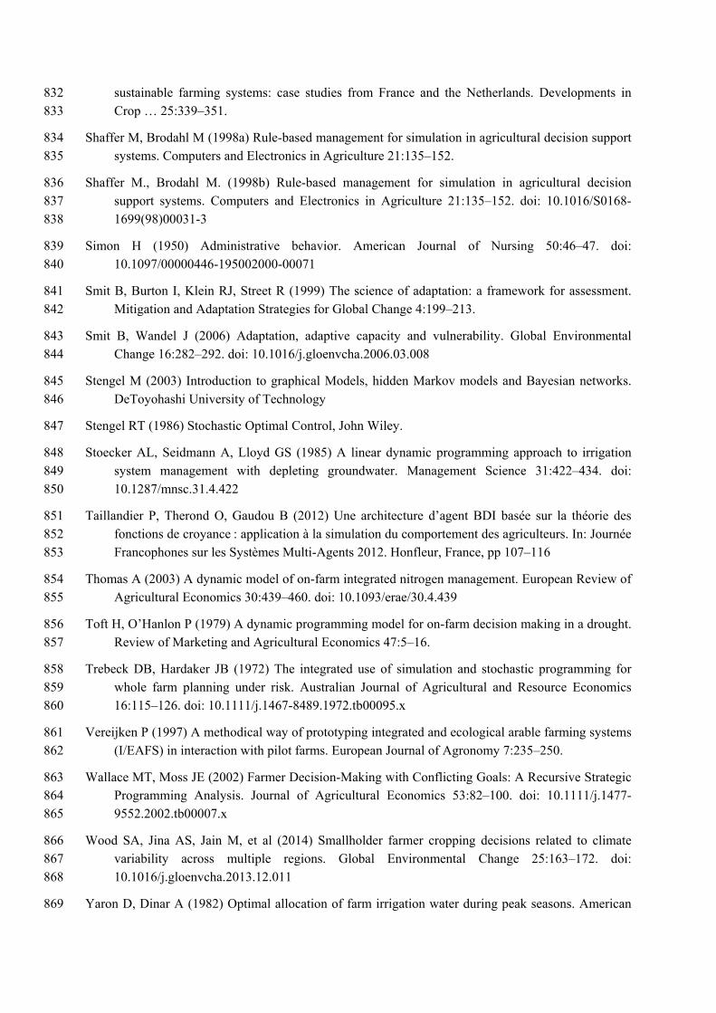
sustainable farming systems: case studies from France and the Netherlands. Developments in 832 Crop … 25:339–351. 833

Shaffer M, Brodahl M (1998a) Rule-based management for simulation in agricultural decision support 834 systems. Computers and Electronics in Agriculture 21:135–152. 835

Shaffer M., Brodahl M. (1998b) Rule-based management for simulation in agricultural decision 836 support systems. Computers and Electronics in Agriculture 21:135–152. doi: 10.1016/S0168-837 1699(98)00031-3 838

Simon H (1950) Administrative behavior. American Journal of Nursing 50:46–47. doi: 839 10.1097/00000446-195002000-00071 840

Smit B, Burton I, Klein RJ, Street R (1999) The science of adaptation: a framework for assessment. 841 Mitigation and Adaptation Strategies for Global Change 4:199–213. 842

Smit B, Wandel J (2006) Adaptation, adaptive capacity and vulnerability. Global Environmental 843 Change 16:282–292. doi: 10.1016/j.gloenvcha.2006.03.008 844

Stengel M (2003) Introduction to graphical Models, hidden Markov models and Bayesian networks. 845 DeToyohashi University of Technology 846

Stengel RT (1986) Stochastic Optimal Control, John Wiley. 847

Stoecker AL, Seidmann A, Lloyd GS (1985) A linear dynamic programming approach to irrigation 848 system management with depleting groundwater. Management Science 31:422–434. doi: 849 10.1287/mnsc.31.4.422 850

Taillandier P, Therond O, Gaudou B (2012) Une architecture d’agent BDI basée sur la théorie des 851 fonctions de croyance : application à la simulation du comportement des agriculteurs. In: Journée 852 Francophones sur les Systèmes Multi-Agents 2012. Honfleur, France, pp 107–116 853

Thomas A (2003) A dynamic model of on-farm integrated nitrogen management. European Review of 854 Agricultural Economics 30:439–460. doi: 10.1093/erae/30.4.439 855

Toft H, O’Hanlon P (1979) A dynamic programming model for on-farm decision making in a drought. 856 Review of Marketing and Agricultural Economics 47:5–16. 857

Trebeck DB, Hardaker JB (1972) The integrated use of simulation and stochastic programming for 858 whole farm planning under risk. Australian Journal of Agricultural and Resource Economics 859 16:115–126. doi: 10.1111/j.1467-8489.1972.tb00095.x 860

Vereijken P (1997) A methodical way of prototyping integrated and ecological arable farming systems 861 (I/EAFS) in interaction with pilot farms. European Journal of Agronomy 7:235–250. 862

Wallace MT, Moss JE (2002) Farmer Decision-Making with Conflicting Goals: A Recursive Strategic 863 Programming Analysis. Journal of Agricultural Economics 53:82–100. doi: 10.1111/j.1477-864 9552.2002.tb00007.x 865

Wood SA, Jina AS, Jain M, et al (2014) Smallholder farmer cropping decisions related to climate 866 variability across multiple regions. Global Environmental Change 25:163–172. doi: 867 10.1016/j.gloenvcha.2013.12.011 868

Yaron D, Dinar A (1982) Optimal allocation of farm irrigation water during peak seasons. American 869

Journal of Agricultural Economics 64:681–689. doi: 10.2307/1240577 870

871

872

TABLE CAPTION 873

Table 1: Modeling adaptive decision-making processes in farming systems; typology of the literature 874

according to adaptation dimensions (temporal scope, spatial scope and timing scope) (DSP: discrete 875

stochastic programming; DP: dynamic programming) 876

Adaptation dimensions Authors Year

Formalism type

Formalism Temporal

Scope Spatial Scope

Timing dimension

Strategic decisions (years)

Farm Reactive Barbier and Bergeron 1999 Dynamic Recursive

Farm Reactive Heidhues 1966 Dynamic Recursive

Farm Reactive Domptail and Nuppenau 2010 Dynamic Recursive

Farm Reactive Wallace and Moss 2002 Dynamic Recursive

Tactical decision (season)

Farm Proactive Trebeck and Hardaker 1972 Static DSP

Farm Proactive Kingwell et al. 1993 Static DSP

Farm Proactive Jacquet and Pluvinage 1997 Static DSP

Farm Proactive Adesina and Sanders 1991 Static DSP

Farm Proactive Burt 1993 Static DSP

Farm Proactive Maatman and Schweigman

2002 Static DSP

Farm Proactive Ritten et al. 2010 Static DSP

Farm Proactive Detlefsen and Jensen 2007 Static Flexible crop-sequence

Farm Proactive Castellazzi et al. 2008 Static Flexible crop-sequence

Farm Proactive Dury 2011 Static Flexible crop-sequence

Tactical decision (daily)

Plot Proactive Ripoche et al. 2011 Static Optional execution

Plot Proactive Martin et al. 2011 Static Optional execution

Plot Proactive Chardon et al. 2012 Static Optional execution

Plot Proactive Martin et al. 2011 Static Optional execution

Plot Proactive McKinion et al. 1989 Static Proactive adjustments

Plot Proactive Ripoche et al. 2011 Static Proactive adjustments

Plot Proactive Martin et al. 2011 Static Proactive adjustments

Plot Proactive Chardon et al. 2012 Static Proactive adjustments

Plot Proactive Rodriguez et al. 2011 Static Proactive adjustments

Plot Proactive Shaffer and Brodahl 1998 Static Time windows

Plot Proactive Cros et al. 1999 Static Time windows

Plot Proactive Crespo et al. 2011 Static Time windows

Plot Proactive Martin et al. 2011 Static Time windows

Strategic & tactical decision (years & season)

Farm & Plot

Reactive Reynaud 2009 Dynamic DP

Farm & Plot

Reactive Stoecker et al. 1985 Dynamic DP

Farm & Plot

Reactive Bryant et al. 1993 Dynamic DP

Farm & Reactive Duffy and Taylor 1993 Dynamic DP

Plot

Farm & Plot

Reactive Fafchamps 1993 Dynamic DP

Farm & Plot

Reactive Hyytiäinen et al. 2011 Dynamic DP

Farm & Plot

Reactive Bontems and Thomas 2000 Dynamic DP

Farm & Plot

Reactive Thomas 2003 Dynamic DP

Farm & Plot

Reactive Pandey and Medd 1991 Dynamic DP

Farm & Plot

Reactive Yaron and Dinar 1982 Dynamic DP

Farm & Plot

Reactive Toft and O’Hanlon 1979 Dynamic DP

Farm & Plot

Reactive & Proactive

Mosnier et al. 2009 Dynamic & Static

Recursive & DSP

Farm & Plot

Reactive & Proactive

Belhouchette et al. 2004 Dynamic & Static

Recursive & DSP

Farm & Plot

Reactive & Proactive

Lescot et al. 2011 Dynamic & Static

Recursive & DSP

877

FIGURE CAPTION 878

879

1: Typology of models to manage adaptive decision-making processes according to model type, 880

approach, and formalism. 881

882

883

884

Figure 1 885