Processes and Threads - Sabancı...
34
1 Scheduling Yücel Saygın |These slides are based on your text book and on the slides prepared by Andrew S. Tanenbaum
Transcript of Processes and Threads - Sabancı...
1
Scheduling
Yücel Saygın |These slides are based on your text book and on the slides
prepared by Andrew S. Tanenbaum
2
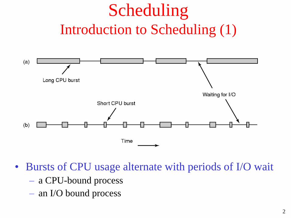
Scheduling Introduction to Scheduling (1)
• Bursts of CPU usage alternate with periods of I/O wait
– a CPU-bound process
– an I/O bound process
3
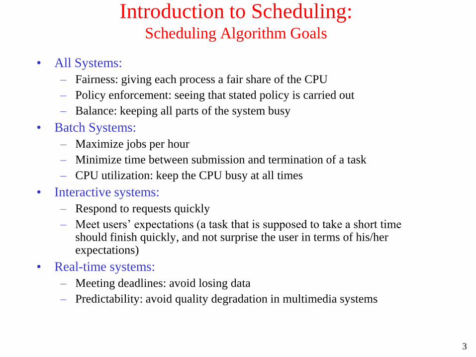
Introduction to Scheduling: Scheduling Algorithm Goals
• All Systems:
– Fairness: giving each process a fair share of the CPU
– Policy enforcement: seeing that stated policy is carried out
– Balance: keeping all parts of the system busy
• Batch Systems:
– Maximize jobs per hour
– Minimize time between submission and termination of a task
– CPU utilization: keep the CPU busy at all times
• Interactive systems:
– Respond to requests quickly
– Meet users’ expectations (a task that is supposed to take a short time should finish quickly, and not surprise the user in terms of his/her expectations)
• Real-time systems:
– Meeting deadlines: avoid losing data
– Predictability: avoid quality degradation in multimedia systems
4
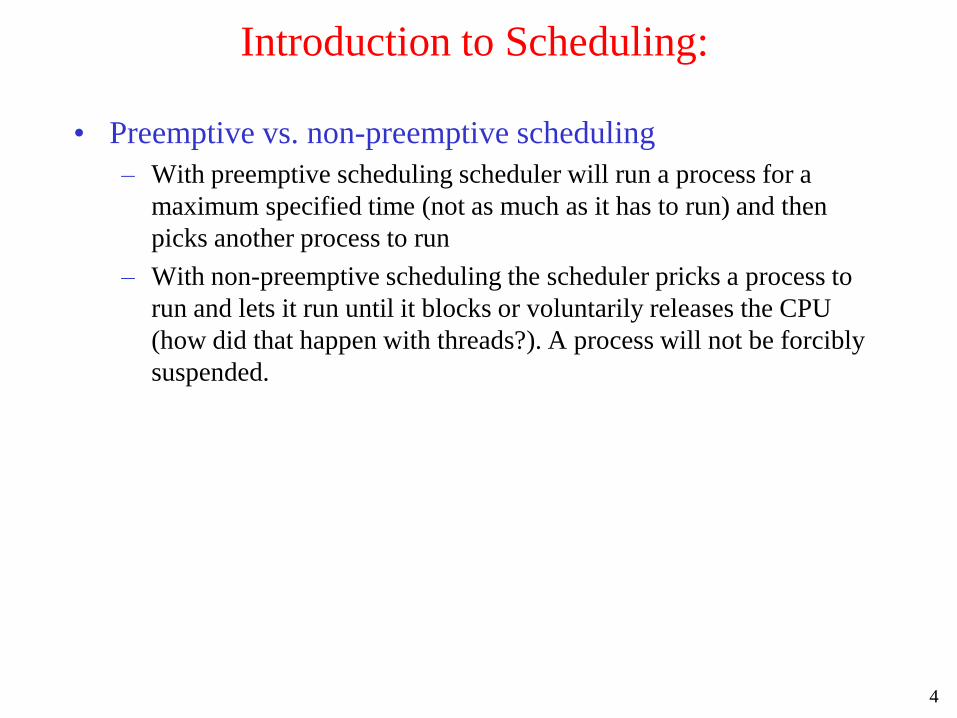
Introduction to Scheduling:
• Preemptive vs. non-preemptive scheduling
– With preemptive scheduling scheduler will run a process for a
maximum specified time (not as much as it has to run) and then
picks another process to run
– With non-preemptive scheduling the scheduler pricks a process to
run and lets it run until it blocks or voluntarily releases the CPU
(how did that happen with threads?). A process will not be forcibly
suspended.
5
Introduction to Scheduling (2)
• Current Systems usually run a mix of batch, (soft) real-
time, interactive
• Therefore it is essential to understand the issues in all such
systems individually.
6
Scheduling in Batch Systems (1)
• Two important parameters:
– Turnaround time: statistical average of time from the moment a
batch job is submitted till the moment it is completed (less is
better)
– Throughput : number of jobs per unit time that the system
completes (usually an hour, and more is better)
• Scheduling algorithm that maximizes throughput may not
necessarily minimize turnaround time
– Ex: running short jobs only, and never running the long jobs will
maximize throughput but induce terrible turnaround time for long
jobs (making the turnaround time infinite in the long run)

7
Scheduling in Batch Systems (1) • First-Come First-Served:
– Assign the the CPU to processes in the order requested
– A single queue of ready processes, as the jobs come in, they are put onto the end of the queue.
– When the running process blocks, the first process (in the ready queue) is run next
– When a blocked process becomes ready, it is appended at the end of the queue (like a new coming process)
• Advantages:
– Very simple to understand, easy to implement with a single queue
– Fair (in the sense that early bird catches the worm)
• Disadvantage:
– Consider I/O bound processes that use little CPU but have to perform 1000 disk reads to complete, and one big CPU bound process that runs for 1 sec and reads a disk block continuously.
– With FCFS, I/O bound processes will finish in 1000 seconds (will all quickly finish using CPU, and wait for the CPU bound process for a second after each disk read)

8
Scheduling in Batch Systems (1)
• Shortest Job First
– Assumes that the running times of jobs can be predicted (e.g.
taking the backup of a 1GB database to the tape, reading 100
records from the database)
– The scheduler picks the shortest job and assigns the CPU to that
job.
9
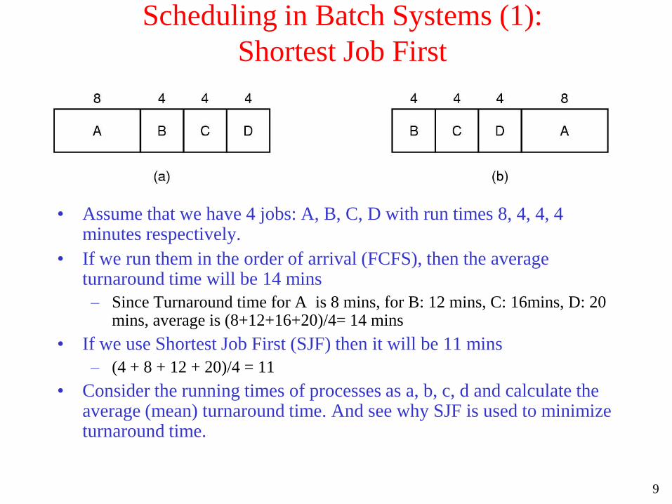
Scheduling in Batch Systems (1):
Shortest Job First
• Assume that we have 4 jobs: A, B, C, D with run times 8, 4, 4, 4 minutes respectively.
• If we run them in the order of arrival (FCFS), then the average turnaround time will be 14 mins
– Since Turnaround time for A is 8 mins, for B: 12 mins, C: 16mins, D: 20 mins, average is (8+12+16+20)/4= 14 mins
• If we use Shortest Job First (SJF) then it will be 11 mins
– (4 + 8 + 12 + 20)/4 = 11
• Consider the running times of processes as a, b, c, d and calculate the average (mean) turnaround time. And see why SJF is used to minimize turnaround time.
10
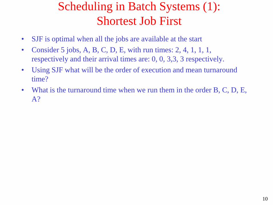
Scheduling in Batch Systems (1):
Shortest Job First
• SJF is optimal when all the jobs are available at the start
• Consider 5 jobs, A, B, C, D, E, with run times: 2, 4, 1, 1, 1,
respectively and their arrival times are: 0, 0, 3,3, 3 respectively.
• Using SJF what will be the order of execution and mean turnaround
time?
• What is the turnaround time when we run them in the order B, C, D, E,
A?
11
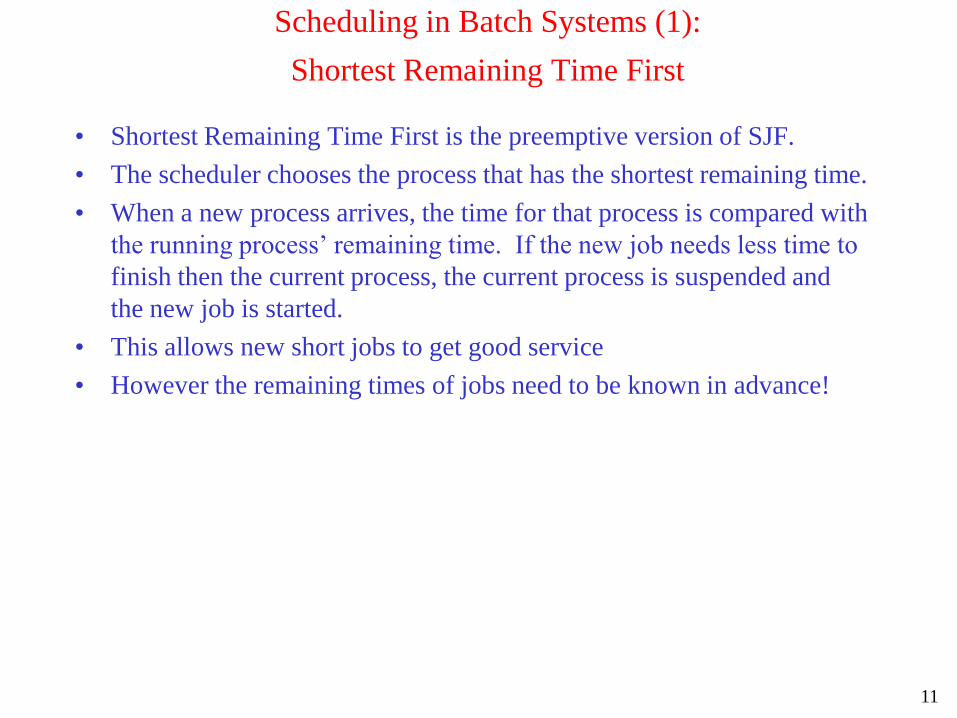
Scheduling in Batch Systems (1):
Shortest Remaining Time First
• Shortest Remaining Time First is the preemptive version of SJF.
• The scheduler chooses the process that has the shortest remaining time.
• When a new process arrives, the time for that process is compared with
the running process’ remaining time. If the new job needs less time to
finish then the current process, the current process is suspended and
the new job is started.
• This allows new short jobs to get good service
• However the remaining times of jobs need to be known in advance!
12
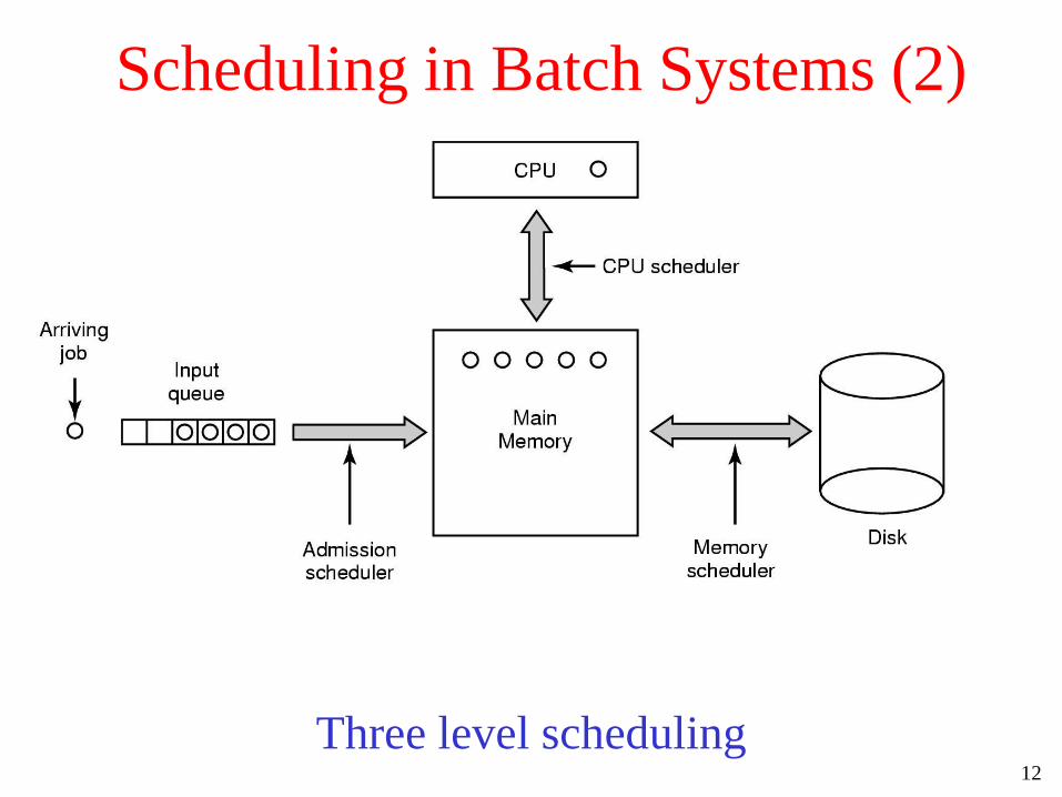
Scheduling in Batch Systems (2)
Three level scheduling
13
Three Level Scheduling (Cont’d)
• Admission Scheduler
– Submitted jobs are kept in the input queue
– Admission Scheduler decides which job to admit to the system
– Usually accepts a mix of I/O and CPU bound processes to keep all parts of the system busy
• Memory Scheduler
– Decides which processes should be kept in memory and which ones in disk
– Decides on the Degree of multiprogramming (number of processes in main memory) and maintains a mix of I/O CPU bound processes in memory
– Tries to achieve a fair allocation of memory
• CPU scheduler
– Is the scheduler that we speak about in general
14
Scheduling in Interactive Systems (1)
• Only two levels of scheduling are used (memory and CPU
scheduling)
• CPU Scheduling is the main focus and we will see the following
scheduling algorithms
– Round Robin Scheduling
– Priority Scheduling
– Multiple Queues (a hybrid of round robin and priority scheduling)
– Shortest process next
– Guaranteed Scheduling
– Lottery Scheduling
– Fair-share scheduling

15
Scheduling in Interactive Systems :
Round Robin Scheduling
– RR Scheduling is simple, fair, and the most widely used scheduling algorithm
– There is a list of runnable processes maintained as a queue
– Each process is assigned a a time interval (called its quantum) for which it is allowed to
run
– A process using the CPU is preempted if it used up its quantum (note that a process may
be blocked say for I/O, before its quantum has elapsed)
– The queue structure is shown in the figure
– Figure (a) depicts the case when B is still running
– Figure (b) shows the queue after B used all its quantum (or blocked for I/O) and
preempted by the scheduler

16
Scheduling in Interactive Systems :
Round Robin Scheduling
• The length of the quantum is an important parameter for RR
scheduling
• Switching from one process to another (context switch) requires some
administrative work (saving, loading registers, flushing/reloading the
cache, updating various tables, lists etc)
• Suppose quantum is 4 msec, and context switch takes 1 msec, then
20% of the CPU time is wasted for administrative overhead.
• Setting the quantum to 99 msec cause only 1% of the CPU to be
wasted but this is too high in interactive systems (consider 10 people
using the system in a queue, the last one will get a chance to get a
response after 1 sec is all the processes fully use their quantum)
• 20-50 msec quantum time seems to be a reasonable compromise

17
Scheduling in Interactive Systems :
Priority Scheduling
• Each process is assigned a priority
• A runnable process with the highest priority is allowed to
run
– Ex: a daemon process sending an email in the background should
have a lower priority than a process displaying a film in real time
• Priorities could be assigned
– statically
– Or dynamically (e.g., giving higher priority to I/O bound processes
that use little CPU, 1/f is a good heuristic where f is the fraction of
the last quantum the process used)
18
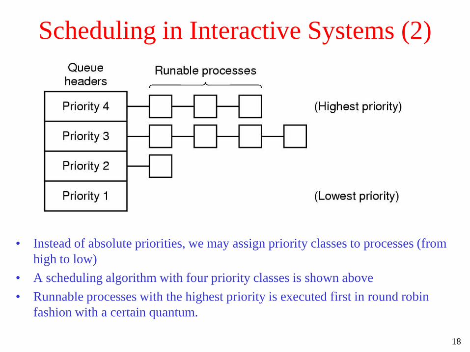
Scheduling in Interactive Systems (2)
• Instead of absolute priorities, we may assign priority classes to processes (from
high to low)
• A scheduling algorithm with four priority classes is shown above
• Runnable processes with the highest priority is executed first in round robin
fashion with a certain quantum.
19
Scheduling in Interactive Systems :
Priority Scheduling
• With priority scheduling, low priority jobs may starve. To
prevent this:
– The priority of the running process may be decreased at each clock
tick
– Processes may have a quantum during which they are allowed to
run. When the current process uses up its quantum, next higher
priority process is scheduled.
20
Scheduling in Interactive Systems :
Priority Scheduling with multiple queues (CTSS system)
• CTSS (Compatible Time Sharing System), One of the earliest (1963)
experiments in the design of interactive time-sharing operating systems, can be
considered as the ancestor of Multics and Unix.
• Memory could hold only one process, so switching from one process to the
other was slow
• To decrease the number of swaps for long running processes,
• priority classes were defined (a queue for each class)
• Processes in the highest priority class could run for one quantum, in the
second highest priority class, for 2 quanta, next higher, 4 quanta, next
higher 8 quanta, and son on.
• A new process starts at the highest priority level and each time it uses all
the quanta allocated to it, it is moved down one class.
• Long processes run less frequently for longer quanta. This way short
interactive processes would be favored for CPU assignment.
• Whenever “enter” was typed at a terminal, the process was assumed to be
interactive, and moved to the highest class, at the end people abused this by
pressing enter all the time.
21
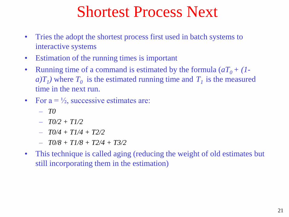
Shortest Process Next
• Tries the adopt the shortest process first used in batch systems to
interactive systems
• Estimation of the running times is important
• Running time of a command is estimated by the formula (aT0 + (1-
a)T1) where T0 is the estimated running time and T1 is the measured
time in the next run.
• For a = ½, successive estimates are:
– T0
– T0/2 + T1/2
– T0/4 + T1/4 + T2/2
– T0/8 + T1/8 + T2/4 + T3/2
• This technique is called aging (reducing the weight of old estimates but
still incorporating them in the estimation)
22
Guaranteed Scheduling
• Tries to give a fair share of CPU to each process (i.e 1/N of the CPU
time to each process if there are N processes)
• Computes the ratio of actual CPU time used to the CPU time that the
process should have been assigned (for a fair CPU assignment)
• Runs the process with the lowest ration until the ratio moves above its
closest competitor.
23
Lottery Scheduling
• Gives processes lottery tickets for CPU time.
• Whenever a scheduling decision is going to be made, a ticket is drawn randomly, and the process that owns the ticket is allowed to use the CPU.
• Processes with more tickets have a higher chance of running.
• Cooperating processes may exchange tickets if they wish (for example a client process may give its tickets to the server to finish its job quickly)
• Very handy for resource allocation
– For example when client processes need different frame rates from a video server such as 10, 20, and 25 frames/sec/ By allocating these processes 10, 20, and 25 tickets, respectively will automatically divide the CPU approximately the correct proportion

24
Fair-Share Scheduling
• Takes into account the owner of the process when
scheduling
• CPU time is shared among the users fairly (otherwise a
user with many processes would have most of the CPU
time)
• Eg: User 1 has 4 processes, A, B, C, D, and user 2 has 1
process E. Then with round robin scheduling the execution
sequence would be:
– A E B E C E D E …..
25
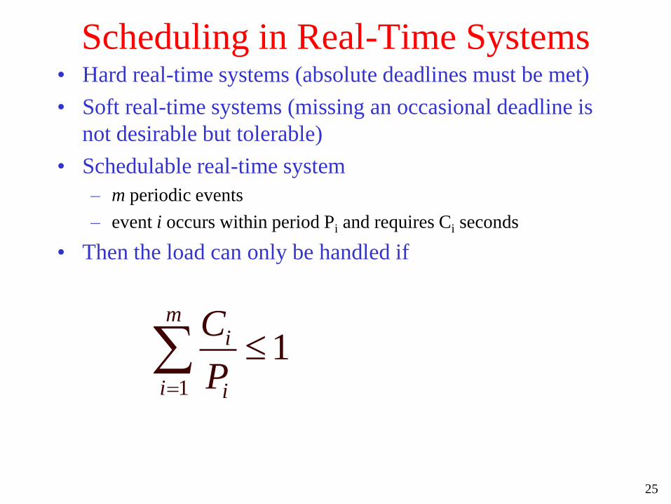
Scheduling in Real-Time Systems • Hard real-time systems (absolute deadlines must be met)
• Soft real-time systems (missing an occasional deadline is
not desirable but tolerable)
• Schedulable real-time system
– m periodic events
– event i occurs within period Pi and requires Ci seconds
• Then the load can only be handled if
1
1m
i
i i
C
P

26
Scheduling in UNIX • Uses Fair-Share Scheduling
• Gives pre-specified rate of system resources to a related set of users.
• Specific users are assigned to fair share groups (ex. TA, Professor)
• Distributes unused resources by one fair share group to other fair share groups wrt their relative needs
System Resources
|Fair Share Scheduler
Process
Scheduler
Group3 Group2 Group1
Process
Scheduler
Process
Scheduler
100%
50% 25% 25%
27
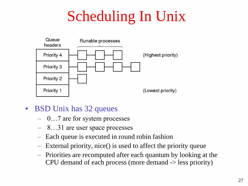
Scheduling In Unix
• BSD Unix has 32 queues
– 0…7 are for system processes
– 8…31 are user space processes
– Each queue is executed in round robin fashion
– External priority, nice() is used to affect the priority queue
– Priorities are recomputed after each quantum by looking at the CPU demand of each process (more demand -> less priority)
28
Scheduling Mechanism of Linux
• (http://www.oreilly.com/catalog/linuxkernel/chapter/ch10.html)
• Each process has a quantum and priority associated with it
• Linux (like all Unix kernels) implicitly favors I/O-bound processes
over CPU-bound ones.
• In order to select a process to run, the Linux scheduler must consider
the priority of each process. Actually, there are two kinds of priority:
– Static priority assigned by the users to real-time processes and ranges
from 1 to 99. It is never changed by the scheduler.
– Dynamic priority (applies only to conventional processes); it is essentially
the sum of the base time quantum (which is therefore also called the base
priority of the process) and of the number of ticks of CPU time left to the
process before its quantum expires in the current epoch.
• The static priority of a real-time process is always higher than the
dynamic priority of a conventional one: the scheduler will start running
conventional processes only when there is no real-time process in a TASK_RUNNING state.
29
Process Preemption in Linux
• http://www.oreilly.com/catalog/linuxkernel/chapter/ch10.html
• The Linux kernel is not preemptive, which means that a process can be
preempted only while running in User Mode;
• Therefore Linux is not a “real” real-time operating system
• nonpreemptive kernel design is much simpler, since most
synchronization problems involving the kernel data structures are
easily avoided
• Process preemption (for processes running in user mode):
– When a process becomes ready to run, kernel checks whether the dynamic
priority of the new process is greater than the priority of the running process. If it is, the execution of current is interrupted and the scheduler
is invoked to select another process to run (usually the process that just
became runnable).
– process may also be preempted when its time quantum expires

30
Process Scheduling in Linux
• http://www.oreilly.com/catalog/linuxkernel/chapter/ch10.html
• The Linux scheduling algorithm works by dividing the CPU time into
epochs.
• In a single epoch, every process has a specified time quantum
computed when the epoch begins. Different processes may have
different time quantum durations.
• When a process has exhausted its time quantum, it is preempted and
replaced by another runnable process.
• A process can be selected several times from the scheduler in the same
epoch, as long as its quantum has not been exhausted--for instance, if it
suspends itself to wait for I/O, it preserves some of its time quantum
and can be selected again during the same epoch.
• The epoch ends when all runnable processes have exhausted their
quantum; in this case, the scheduler algorithm recomputes the time-
quantum durations of all processes and a new epoch begins.

31
Process Scheduling in Linux
• http://www.oreilly.com/catalog/linuxkernel/chapter/ch10.html
• The users can change the time quantum of their processes by using the nice( ) and setpriority( ) system calls
• A new process always inherits the base time quantum (the time
quantum assigned at the beginning of the epoch) of its parent.
32
Policy versus Mechanism
• Separate what is allowed to be done with how it is done
– a process knows which of its children threads are important and need priority
• Scheduling algorithm parameterized
– mechanism in the kernel
• Parameters filled in by user processes
– policy set by user process

33
Thread Scheduling (1)
Possible scheduling of user-level threads
• 50-msec process quantum
• threads run 5 msec/CPU burst
34
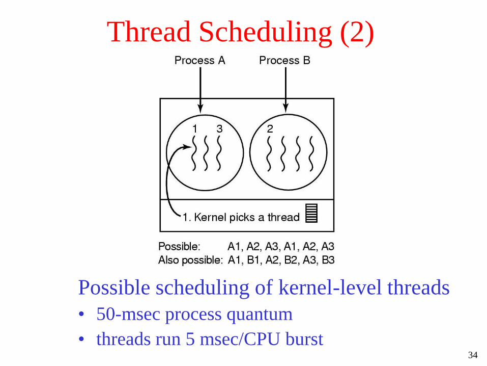
Thread Scheduling (2)
Possible scheduling of kernel-level threads
• 50-msec process quantum
• threads run 5 msec/CPU burst