Process flowsheet optimization : recent results and future directions
31
Carnegie Mellon University Research Showcase @ CMU Department of Chemical Engineering Carnegie Institute of Technology 1987 Process flowsheet optimization : recent results and future directions Lorenz T. Biegler Carnegie Mellon University Carnegie Mellon University.Engineering Design Research Center. Follow this and additional works at: hp://repository.cmu.edu/cheme is Technical Report is brought to you for free and open access by the Carnegie Institute of Technology at Research Showcase @ CMU. It has been accepted for inclusion in Department of Chemical Engineering by an authorized administrator of Research Showcase @ CMU. For more information, please contact [email protected].
Transcript of Process flowsheet optimization : recent results and future directions
Carnegie Mellon UniversityResearch Showcase @ CMU
Department of Chemical Engineering Carnegie Institute of Technology
1987
Process flowsheet optimization : recent results andfuture directionsLorenz T. BieglerCarnegie Mellon University
Carnegie Mellon University.Engineering Design Research Center.
Follow this and additional works at: http://repository.cmu.edu/cheme
This Technical Report is brought to you for free and open access by the Carnegie Institute of Technology at Research Showcase @ CMU. It has beenaccepted for inclusion in Department of Chemical Engineering by an authorized administrator of Research Showcase @ CMU. For more information,please contact [email protected].
NOTICE WARNING CONCERNING COPYRIGHT RESTRICTIONS:The copyright law of the United States (title 17, U.S. Code) governs the makingof photocopies or other reproductions of copyrighted material. Any copying of thisdocument without permission of its author may be prohibited by law.
PROCESS FLOWSHEET OPTIMIZATION:RECENT RESULTS AND FUTURE DIRECTIONS
by
L T. Biegler
EDRC-06-27-87
PROCESS FLOWSHEET OPTIMIZATION STRATEGIES:
RECENT RESULTS AND FUTURE DIRECTIONS
L. T. BieglerChemical Engineering Department
Carnegie-Mellon UniversityPittsburgh, PA 15213
Optimization strategies based on detailed and rigorous models of
process flowsheets have been of interest to process engineers for the
past 25 years. Here we review earlier optimization strategies and
emphasize more recent strategies based on Successive Quadratic
Programming (SQP). These strategies allow the simultaneous solution and
optimization of the process model and thus lead to significant
reductions in the computational effort for an optimization study.
Several examples are presented to define the optimization problem and
demonstrate the performance of the simultaneous strategies. Finally,
some open research questions are described and future directions in
process optimization are briefly discussed.
Key words: Flowsheeting, Process Simulation, Process Optimization,
Nonlinear Programming, Successive Quadratic Programming
Abbreviated Title: FLOWSHEET OPTIMIZATION STRATEGIES
University LibrariesCarnegie Mellon University
Pittsburgh, Pennsylvania 15213
SUMMARY
Application of Successive Quadratic Programming strategies to
process optimization has reduced the computational effort by more than
an order of magnitude over conventional methods and now creates the
potential to make simulator-based optimization with complex process
models a powerful tool. This report describes the process optimization
problem with a simple flowsheeting model and briefly discusses the
infeasible path approach, which permits simultaneous recycle
convergence and optimization with SQP. Several improvements to the
infeasible path algorithm are then outlined that include better gradient
calculation and scaling strategies, a more efficient line search function
and more reliable performance through intermediate recycle convergence.
These concepts are applied to a large-scale process problem and
resulting improvements are demonstrated. Finally, we present a brief
discussion of open research questions and directions for future research.
INTRODUCTION
With the application of computers in process engineering,
flowsheet models, i.e. steady-state process models of chemical
processes, have been developed and widely used in the chemical
industry. These flowsheeting packages or process simulators very
successfully predict the accurate behavior of a process' steady-state
behavior, and are flexible in describing general-purpose processes. A
number of process simulators are widely used by chemical and
engineering companies (see [21] for a comprehensive list.), and these
find frequent use in evaluating and improving proposed process designs,
monitoring and analyzing the performance of existing designs and in
guiding the redesign or retrofit of inefficient existing processes.
The structure of these simulators is highly modular and this makes
it easy for the engineer to quickly set up a flowsheet and choose a set
of physical property and equipment performance models of appropriate
accuracy and complexity. Almost all commercial process simulators have
a structure that is termed sequential modular. Here, instead of
specifying the full process model as a single set of nonlinear equations
that need to be solved, calculation usually proceeds in the same way
that material flows in the process. Process equations are grouped
according to the particular unit operation they describe and require
inputs that characterize the normal operating behavior of a process. For
example, simulators require that the flowrates of raw materials be
specified rather that the production rate. While this mode allows for the
easy construction, modification and use of process simulators, the rigid
input-output strategy also leads to inefficient calculation strategies for
design and optimization. For example, almost all chemical processes
require recycle streams to achieve high conversion of raw material to
streams and input equipment parameters. This may, of course, require
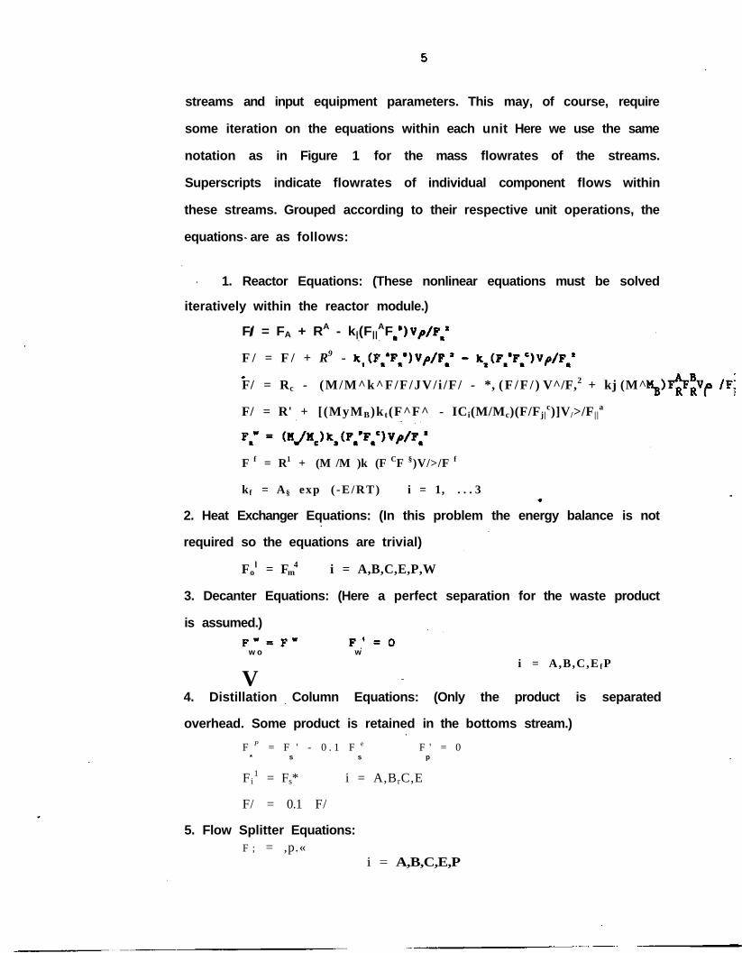
some iteration on the equations within each unit Here we use the same
notation as in Figure 1 for the mass flowrates of the streams.
Superscripts indicate flowrates of individual component flows within
these streams. Grouped according to their respective unit operations, the
equations are as follows:
1. Reactor Equations: (These nonlinear equations must be solved
iteratively within the reactor module.)
F/ = FA + RA - k|(F||AF/
F / = F / + R9 -
F/ = Rc - (M/M^k^F/F/JV/ i /F / - *, ( F / F / ) V^/F,2 + kj (M^
F/ = R' + [(MyMB)k t(F^F^ - ICi(M/Mc)(F/Fj|c)]V/>/F||
a
F f = R1 + (M /M )k (F CF §)V/>/F f
kf = A§ exp ( - E / R T ) i = 1, . . . 3
2. Heat Exchanger Equations: (In this problem the energy balance is not
required so the equations are trivial)
Fol = Fm
4 i = A,B,C,E,P,W
3. Decanter Equations: (Here a perfect separation for the waste product
is assumed.)
w o wi = A,B,C,E f P
V4. Distillation Column Equations: (Only the product is separated
overhead. Some product is retained in the bottoms stream.)
F P = F ' - 0 . 1 F e F ' = 0* s s p
F i1 = Fs* i = A,B rC,E
F/ = 0.1 F/
5. Flow Splitter Equations:F ; = ,p.«
i = A,B,C,E,P
6. Recycle (or Tear) Equations: (In all sequential modular simulators,
these tear equations complete the mass balance and make up the outer
calculation loop.)
R1 - Rfl = 0 i = A,B,C,D,E,P
The objective function is given in terms of the net sales minus
fixed charge, raw material, utility and waste disposal costs. This is
normalized by the plant investment cost to give an annual rate of
return. Using the cost coefficients, C., in [23] gives the following
objective function:
Additional kinetic parameters as well as more information on the
objective function can be found in the supporting references
[1,9,11,17,20,23]. In addition, the following inequality constraints are
imposed:
580 <> T < 680
0 £ Fp < 4763
nonnegativity on all flows
For fixed feeds and p. any three of the above variables can be
selected as decision variables for optimization. Because the above
models are restricted to input-output form, however, only certain
decision variables are available. For this example a typical choice of
decisions is reactor temperature (T), reactor volume (V) and split fraction
(if). We denote this vector of decision variables x.
Note that the simple models given above can be replaced module
by module by much more complex ones without disturbing the other
modules or the overall calculation sequence of the flowsheet. It is easy
to see that with complicated thermodynamic and unit operations models,
the simulation may consist of many thousands of variables and
equations that may be totally transparent to the user. In fact, the only
variables that need to be known for overall flowsheet convergence are
the recycle flow rates. We denote the vector of tear variables (R) as y,
the corresponding calculated variables (FT) as w(y) and define the
flowsheet convergence problem as:
Solve: h(y) = y - w(y) = 0
Since all other variables need not be accessed explicitly and
equations are buried within their appropriate models, only very simple
algorithms (such as direct substitution) are generally applied for recycle
convergence. The structure of the optimization problem is therefore:
Max
s.t. g(x) < 0
where it is required that the equations h(y) = 0 are solved for
every evaluation of the functions jt(x) and g(x).
Typically a process optimization problem with the above structure
can be very time-consuming to solve if complex process models are
used. Early studies applied direct search methods (e.g. Hooke-Jeeve,
Complex search or adaptive random search) to the flowsheet and
required up to several hundred simulation time equivalents to come
close to an optimal solution [1,10,11,13,14,20,23,27]. Friedman and
8
Pinder [13] also applied more sophisticated gradient-based strategies to
the flowsheet and found only marginal improvements in performance.
Here in order to calculate gradients, a decision variable is perturbed and
the entire flowsheet is reconverged. Because of slowly converging
recycle solvers, however, this procedure can be very inefficient. Also,
typically loose error tolerances will corrupt the accuracy of the
gradients and lead to poor performance. To get around these problems
with "feasible path" or "black-box" optimization strategies, we develop
a more recent strategy based on reformulating the process optimization
problem.
Infeasible Path Optimization
Instead of considering the simulation problem as a black box, we
would like to incorporate the recycle convergence equations directly into
the optimization problem. By formulating the problem as:
Min ^(x,y)
s.t. g(x,y) j£ 0h(x,y) = y - w(x,y) = o
we have combined the optimization loop and the most slowly
converging calculation loop. This occurs of course at the expense of
increasing the size of the optimization problem. To solve this nonlinear
programming problem, we choose an algorithm that requires few
function calls (these require evaluation of complex flowsheet models)
and does not need to converge the equality constraints completely for
intermediate function evaluations.
Here, the Successive Quadratic Programming (SQP) algorithm
appears to be the method of choice. Numerous studies indicate (see
[16,22]) that it generally requires the fewest function evaluations. Also,
inequality and equality constraints are linearized at each iteration and
converge as progress is made toward the optimum. To illustrate this
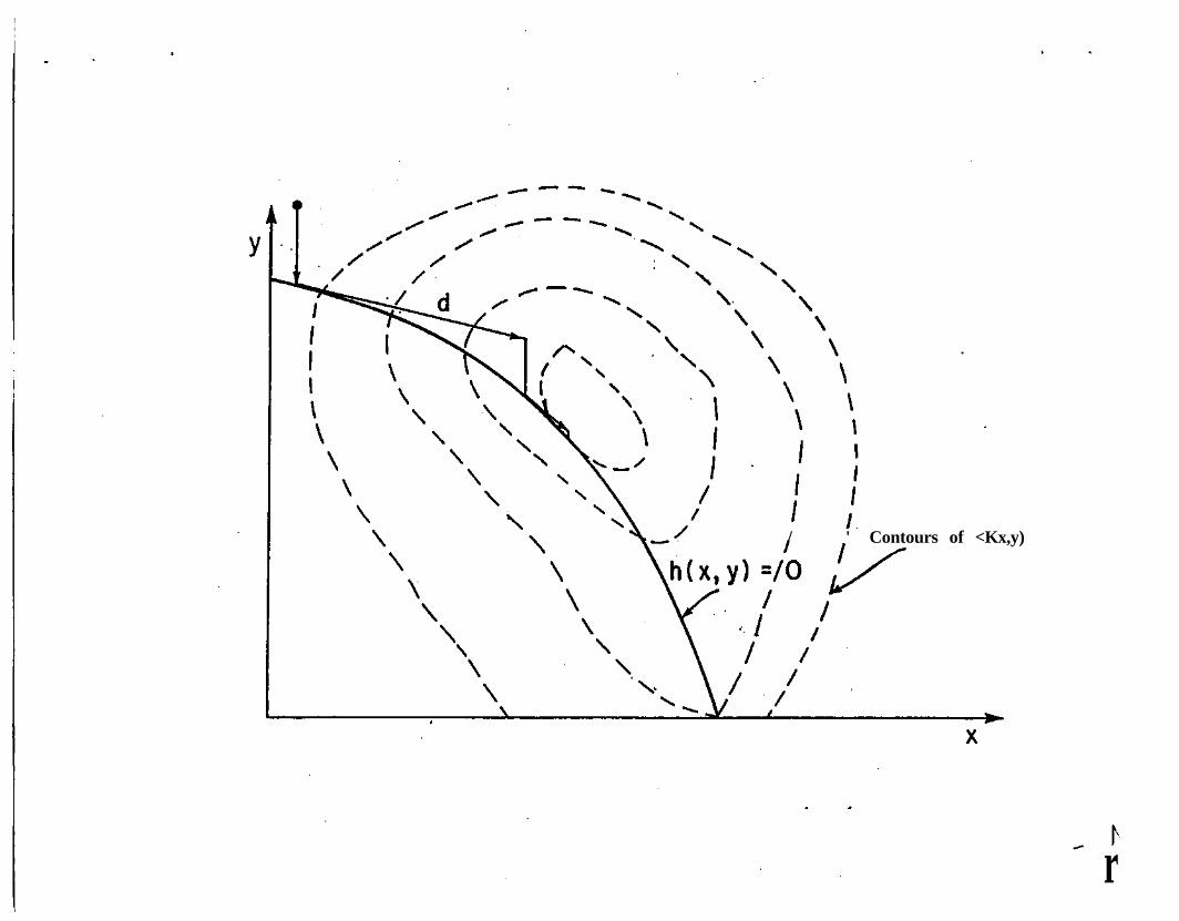
method in the context of flowsheet optimization, consider the contour
plot in Fig. 2a. Here we consider an idealized flowsheet in the space of
x and y where the tear constraint, h(x,y) = 0 is represented as a solid
line. With the "black box" approach the optimization proceeds in the
space of x and the simulation operates in the space of y with x fixed,
as seen in Fig. 2a. Note that the vertical steps in this figure represent
computationally expensive simulations. On the other hand, the infeasible
path approach with SQP requires setting up and solving the following
quadratic program at each iteration:
mind
s.t . g(x*,y') + Vg(x',y')Td < o
h(x',y4) + Vh(xf,y')Td = 0
in the space of x and y. The solution of the quadratic program
determines a search direction, d. A line search that minimizes some
merit function determines a step size along this direction for the next
point. To construct the quadratic program, function and gradient
information must be evaluated from the flowsheet. These require single
flowsheet passes for each function evaluation or gradient perturbation.
The Hessian matrix, B, is approximated using quasiHMewton updating
formulae and needs no additional information from the flowsheet.
Kaijaluoto [17] applied this strategy to the Williams-Otto process
in the previous section, and required less than 10 equivalent simulation
times to optimize the process. In previous studies several hundred
simulation time equivalents were typically required. Even from poor
starting points (as given in [23]) we found this strategy to perform
efficiently and reliably on this problem.
10
However, a number of issues need to be considered in
implementing this approach to more complex process models.
Performance of the strategy can be influenced by methods for
calculating gradients, problem scaling, and the choice of the merit
function used in the SQP algorithm. Moreover, some safeguards need to
be enforced because the infeasible path method may choose a point
which may cause an error in the simulator. Such a failure can be
disastrous as the user is then left with neither an optimal nor a feasible
point. These issues are explored in the next section.
IMPROVEMENTS AND ENHANCEMENTS TO THE INFEASIBLE PATH
APPROACH
Here we consider a number of options for improving the
efficiency and reliability of the infeasible path approach. Following this
section we present a process case study that summarizes the effect of
these enhancements.
Gradient Calculation Strategies
The most straightforward way of calculating gradients is simply to
perturb the decision (x) and tear variables (y) and execute a full
flowsheet pass with the recycle streams torn. Some computational
savings can be had by realizing that many of the decision variables
(such as in Fig. 1) require only partial flowsheet perturbations. In the
implementation within the sequencing routine of a process simulator,
this strategy, termed direct loop perturbation [3,5], is very easy to
implement.
A potentially more accurate and efficient strategy requires
gradients to be calculated module by module [3 ] . Here block Jacobians
11
and intermediate gradients can be evaluated for each module and the
desired gradients for the tear and decision variables can be obtained by
chainruling the individual Jacobians. From Figure 1 it is easy to see how
this strategy leads to a reduction in the number of module evaluations.
For example, evaluation of the gradient with respect to reactor volume
requires only perturbation of the reactor module along with chainruling
of existing Jacobians, rather than perturbation of the entire flowsheet.
Improving the accuracy of flowsheet gradients has also been the
subject of several studies [3,5,17]. Here the chainruling strategy offers
an advantage because analytic gradients and Jacobians (which are
available for simple modules) can be substituted for module
perturbations. Also Kaijaluoto [17] considered choosing an appropriate
perturbation size by balancing roundoff and higher order Taylor series
error. Estimation of these errors, however, requires additional flowsheet
perturbations or more knowledge of the process simulation problem.
Finally, an analysis of errors resulting from different gradient calculation
approaches can be found in [ 3 ] .
Choice of a Line Search Function
This aspect of the infeasible path approach is rooted in theoretical
properties of the SQP algorithm. Using an analogy to Newton's method
for solving nonlinear equations, it is often necessary to have some
control over stepsize to enforce global convergence from poor starting
points. Close to the solution, however, the rate of convergence can be
poor if full steps are not taken along the search direction. The original
line search (or merit) function developed for SQP is the exact penalty
function [15,22]:
VI
P(x,y) = ^(x.y) «• *(Ig.(x.y)4 * I | h.(x,y)
where g. (x,y) = max(O,g (x,y)) and a is a penalty parameter. Using
this function to determine a stepsize along a QP-generated search
direction, one is guaranteed, under mild conditions, to converge to at
least a local optimum from any starting point. However, the function
may lead to small stepsizes and slow convergence when close to the
optimum.
Several remedies have been proposed for the problem of slow
convergence. Along with a number of researchers [24], we have
replaced the exact penalty function with an augmented Lagrange
function:
L'ix.y) = fkx.y) + uJg{x.y\ + vThix.y) + (a/%\ \g^h\ \2
where the multipliers u and v are calculated by the quadratic
program. As shown in [4,24], this function preserves the global
convergence property but also allows full steps to be taken in a
neighborhood about the optimum.
As wil l be illustrated later, the exact penalty function can lead to
poorer performance as the optimum is approached. This is especially
true if errors exist in the gradients and the problem becomes i l l -
conditioned. Because of theoretical properties of the augmented
Lagrange function, we obtain better performance of the algorithm near
the optimum as a result of its accepting full steps generated by the
quadratic program [4 ] .
Scaling of the Optimization Problem
The solution to the quadratic program (QP) at each iteration of

13
SQP is invariant to changes in the scaling of variables or objective and
constraint functions. Moreover, the quasi-Newton updating formula for
calculating the Hessian matrix, B, is also scale invariant. Consequently,
scaling the process optimization problem needs to be motivated by only
two concerns.
First, despite the scale invariance properties of quadratic
programming, gradients may vary over several orders of magnitude and
thus make the problem ill-conditioned. This could lead to QP solutions
that are corrupted by roundoff error. In solving linear equations and
linear programs several variable and function scaling algorithms have
been developed that attempt to improve the conditioning of the
problem. However, numerical tests of these algorithms (see [26]) do
not reveal significant advantages in performance. Instead, the choice of
a good scale factor seems largely to be problem dependent. To deal
with ill-conditioned QP's we calculate the condition number of the B
matrix at each iteration. For high condition numbers we can assume the
problem is poorly scaled and thus rescale to improve performance.
Also, variable scaling can greatly influence performance of SQP
through initialization of the B matrix. Here the B matrix is an estimate
of the Hessian of the Lagrange function and proper initialization should
be based on second derivative information at the starting point. Since
this information is frequently too expensive to calculate, the B matrix is
usually set to the identity matrix, although through variable scaling this
matrix can implicitly be set to some other diagonal, positive definite
form. However, without some knowledge of higher order derivatives,
this choice is arbitrary. To somehow reflect the nature of the problem
variables we have adopted the heuristic of normalizing the variables by
their bounds, once these are chosen appropriately [4]. As will be seen
14
this strategy works well even compared with problems where the scale
factors were chosen by trial and error.
Intermediate Convergence to Aid SQP Performance
As mentioned above, certain safeguards need to be imposed as a
result of moving in an infeasible space. One option that has been
applied with some success is the use of a trust region [12] in the early
stages of the SQP algorithm. Also since the estimate of the Hessian is
initially poor, it seems reasonable to limit the length of the search
direction and let successive points build up the approximation of the
Hessian. Chen and Stadtherr [8] report some numerical tests of this
strategy for process optimization.
Another option is to remain on or close to the feasible space.
Here it is possible to solve the full quadratic program at each iteration
but to apply a few iterations of the recycle convergence algorithm (with
X fixed) before proceeding to the next QP subproblem. A pictorial
representation of this procedure is given in Fig. 2c. The intention, of
course, is that full or partial convergence will improve poor starting
points and lead to fewer iterations. Moreover, since the full QP is
constructed, the gradients with respect to x will be more accurate than
with a "black box" method, where the flowsheet is reconverged for
each perturbation. Biegler and Hughes [7] developed two feasible variant
strategies that use full flowsheet convergence between SQP iterations.
More recently, Kisala et al [18] reported some cases where partial
convergence could be more advantageous than either infeasible path or
full intermediate convergence. Finally, Lang and Biegler [19] developed
an algorithm that includes systematic ways of performing partial
convergence along with a more efficient Broyden convergence algorithm.
15
CASE STUDY OF IMPROVEMENTS TO INFEASIBLE PATH
To demonstrate the effect of some of the improvements described
above, we consider a comprehensive flowsheet optimization problem.
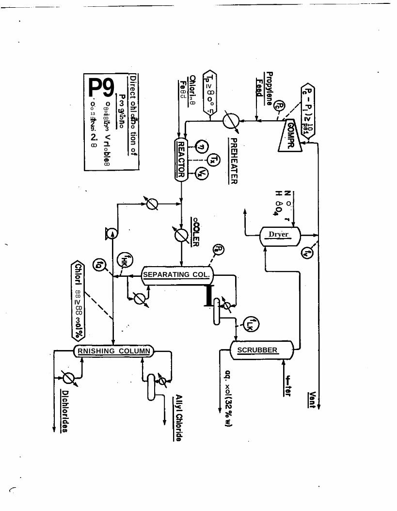
Figure 3 shows a flowsheet for the propylene. chlorination process.
Propylene feed is mixed with the recycle loop and with chlorine feed.
The mixture reacts in gas phase to form allyf chloride as well as
heavier chlorinated products and hydrogen chloride. The reactor effluent
is cooled by a quench loop which also stops the reaction. After further
cooling the stream is separated in a distillation column to remove HCI,
chlorine and propylene overhead. The bottoms product, consisting of
chlorinated compounds, is further separated into allyl chloride product
and dichlorinated byproducts. In the recycle, HCI is recovered in a
scrubber/dryer system from propylene and chlorine as boiling
hydrochloric acid. The remainder is then vented to minimize buildup of
impurities and recycled back to the feed.
This process was simulated on SPAD, a sequential modular
simulator developed at the University of Wisconsin. The process models
were of intermediate complexity and are made up of several hundred
equations. More details of the process model and parameters can be
found in [4,6]. Because the model deals with an existing process the
optimization problem is posed as:
Max {Sales - Raw material}
s . t . product purity £ 99%pressure increase across recycle compressor £ 10 psireactor inlet temperature £ 90 F
mass and energy balances must be satisfied(recycle equations are converged)
Nine decision variables are selected for this optimization problem.
These are indicated by the circled variables in Fig. 3. A complete
16
description of the optimization problem along with starting points,
product prices and performance statistics can be found in [6]. It is
instructive to consider how the performance of the optimization strategy
changes as a result of the improvements described above.
The original application to this flowsheet used the SQP algorithm
with an exact penalty function. A good scaling vector was determined
by trial and error and a direct loop perturbation strategy was used to
calculate the gradients used in the QP. The resulting formulation required
45 simulation time equivalents (STE's) to reach the optimum. With more
careful attention paid to the accuracy of the derivatives the performance
was improved to 34 simulation time equivalents. In the same study, two
feasible variant algorithms were applied. These differed from each other
only slightly and both required convergence of the flowsheet at
intermediate points between SQP iterations. This safeguard allowed
faster convergence and despite the exact penalty line search function
and inefficient derivative calculations, both feasible variant approaches
required the equivalent time of only 29 simulations.
On closer examination of these results, one sees that, while
excellent progress is made initially, several iterations are required in the
neighborhood around the optimum before convergence occurs. This may
be due to inexact gradients and their use in evaluating the Kuhn-Tucker
tolerance, as well as the slow convergence properties of the exact
penalty line search. To remedy this situation the chainruling strategy
outlined above was used for gradient calculation [3]. Here analytic
Jacobians are supplied for mixers, splitters and the compressor units.
Thus, this strategy leads to more accurate derivatives with fewer
module perturbations. The result is that the infeasible path algorithm
now requires only 23 STE's to reach the optimum.
17
Replacing the exact penalty function with the augmented Lagrange
line search function given above also makes a substantial difference.
Because this function allows full SQP steps to be taken in the
neighborhood of the optimum, the slow convergence noted before can
be eliminated. Applied to this problem from the same starting points as
for the previous cases, we now require only 13 equivalent simulation
times for optimization. Finally, as a result of the heuristic scaling
algorithm sketched above, performance of the infeasible path algorithm
is improved even further; only 9 simulation times are required [4].
The improvements demonstrated with this case study, along with
later work on strategies that use partial intermediate convergence [19],
have recently been implemented on the FLOWTRAN process simulator
[25]. Developed by the Monsanto Co. and continously used and
updated since 1966, this simulator has been used widely in industry and
academia, and is currently a valuable teaching tool in many chemical
engineering curricula. The optimization implementation on FLOWTRAN is
fairly transparent to the user, allows easy specification of the process
optimization problem, and is flexible enough to accommodate a number
of optimization strategies including infeasible path with partial or full
intermediate convergence. This implementation has been used to solve
over a dozen new optimization examples as well as the propylene
chlorination problem described above. Some of these examples have
been reported in [19]. Here one sees that the optimization results are
still consistent with the above case study. Even on fairly large
problems we are able to obtain optimal solutions within ten simulation
times.
PROBLEMS FOR FUTURE CONSIDERATION
18
The SQP based optimization strategies described above allow
much more flexibility and efficiency for process flowsheeting. Naturally
this leads to a number of questions that need to be considered for
further improving the optimization strategy. A partial list of these is
given below.
Larger Problems
Many chemical processes involve a large number of chemical
components; including these components in the optimization problem
still may lead to a prohibitive amount of work in calculating gradients.
Here although the "Mack box" strategy may be more efficient than the
infeasible path strategy in this case, both optimization strategies are
too expensive for these problems. An open question is whether
systematic ways exist for combining or eliminating unnecessary
components (e.g. those that do not participate in reactions and are
easily separated) and still guarantee convergence to the flowsheet
optimum.
Modules that have Differential Equation Models
Although these models are self-contained within modules and can
be treated normally, these models can be extremely time-consuming
because they frequently require complex physical property calculations
at each integration step. An example of this occurs when the reactor
model in the Williams-Otto flowsheet is replaced by a packed bed
model. Because of these issues it may be useful to include convergence
of these difficult and time-consuming models in the optimization loop.
Typically, higher order methods can then be applied since they require
fewer integration steps and fewer function evaluations. A preliminary
19
study that outlines this approach is presented in [9]. For models that
require complex thermodynamic calculations, it is demonstrated this
approach has the potential to improve the efficiency by an order of
magnitude.
Formulation of Process Optimization Problems for more Efficient
Solution
The infeasible path optimization strategy is but one way of
improving performance through different and more flexible formulation
of the process problem. In addition, several systematic ways need to be
explored that include exploiting linear functions wherever possible (e.g.
mass balances and stream flows). This reduces the work required for
gradient calculation and by the optimization algorithm. Further knowledge
of the process can be applied in choosing appropriate decision variables
and good initial values for them. Finally, the optimization problem needs
to be modeled so that nondifferentiabilities and discontinuities present
in process and cost functions are avoided or eliminated. Otherwise,
these difficulties can be serious obstacles to obtaining successful
solutions to process optimization problems.
CONCLUSIONS
Compared to earlier strategies which require up to several hundred
equivalent simulation times to reach an optimal solution, SQP-based
strategies offer clear advantages and thus make frequent and efficient
process optimization studies possible. In fact, these methods also offer
the possibility of using fairly rigorous models for the on-line
optimization of operating plants.
After describing the structure of steady-state process optimization
20
problems using a very simple process model, we sketched the
application of the SQP algorithm for simultaneous convergence and
optimization. A number of factors were then considered that led to
improvement of the optimization strategy. These include more efficient
and accurate methods for gradient calculation, better merit functions for
choosing stepsizes and simple, heuristic scaling strategies. In addition,
the advantages of intermediate recycle convergence were outlined.
Recent studies indicate that for poorly initialized starting points and
badly scaled problems, full or partial convergence can lead to more
efficient and reliable performance. Finally, for demonstration purposes,
these concepts have been implemented on FLOWTRAN, a large-scale
commercial process simulator.
However, a number of open questions remain in process
optimization. These include handling problems of large size and model
complexity. Also many questions regarding the appropriate formulation
of process simulator-based problems for more efficient solution have
yet to be explored. These represent interesting and fruitful areas for
future research.
21
REFERENCES
[ 1] Adelman, A. and W.F. Stevens, "Process Optimization by the
Complex Method", AlChE J., 18, 1, p. 20 (1972)
[ 2] Ballman, S. H. and J.L. Gaddy, "Optimization of Methanol
Process by Flowsheet Simulation", I & EC Proc. Oes. Dev., 16, 3, p. 337,
(1977)
[ 3] Biegler, LT., "Improved Infeasible Path Optimization for
Sequential Modular Simulators, Part I: The Interface", Comp. and Chem,
Eng., 9, 3, p. 245, (1985)
[ 4] Biegler, LT. and J.E. Cuthrell, "Improved Infeasible Path
Optimization for Sequential Modular Simulators, Part II: The Optimization
Algorithm", Comp. and Chem. Eng., 9, 3, p. 257, (1985)
[ 5] Biegler, LT. and R.R. Hughes, "Infeasible Path Optimization of
Sequential Modular Simulators" AlChE J., 28, 6, p. 994 (1982)
[ 6] Biegler, LT. and R.R. Hughes, "Optimization of Propylene
Chlorination Process: A Case Study Comparison of Four Algorithms"
Comp. and Chem. Eng., 7, 5, p. 645 (1983)
[ 7] Biegler, LT. and R.R. Hughes, "Feasible Path Optimization for
Sequential Modular Simulators" Comp. and Chem. Eng.# 9, 4, p. 379
(1985)
[ 8] Chen, H-S and M.A. Stadtherr, "A Simultaneous Modular
Approach to Process Flowsheeting and Optimization", AlChE J., 31, 11,
p. 1843, (1985)
22
[ 9] Cuthrell, J.E. and LT. Biegler, "Simultaneous Solution and
Optimization of Process Flowsheets with Differntial Equation Models".
IChemE Symp. Ser. #92, p. 13 (1985)
[10] DiBella, C.W. and W.F. Stevens, "Process Optimization by
Nonlinear Programming", I & EC Proc. Des. Dev., 4, 1, p. 16 (1965)
[11] Findley, M.E., "Modified One-at-a-Time Optimization". AlChE
J., 20, 6, p. 1154 (1974)
[12] Fletcher, R., "Practical Methods of Optimization, Vol. 2,
Constrained Optimization", Wiley & Sons, New York (1981)
[13] Friedman, P. and K.L Pinder, "Optimization of a Simulation of
Chemical Plants", I & EC Proc. Des. Dev., 11, 4, p. 512 (1972)
[14] Gaines, L.D. and J.L Gaddy, "Process Optimization by
Flowsheet Simulation", I & EC Proc. Des. Dev., 15, 1, p. 206 (1976)
[15] Han, S-P, "A Globally Convergent Method for Nonlinear
Programming", J. Opt. Theo. and Appl., 22, 3, p. 297 (1977)
[16] Hock, W. and K. Schittkowski, "Test Examples for Nonlinear
Programming Codes", Lecture Notes in Economics #187, Springer (1981)
[17] Kaijaluoto, S., "Process Optimization by Flowsheet
Simulation" Technical Research Center of Finland, Publication #20 (1984)
[18] Kisala, T.P., ScD Thesis, Massachusetts Institute of
Technology, Cambridge, MA (1985)
[19] Lang, Y-D and L.T. Biegler, "A Unified Algorithm for
Flowsheet Optimization", submitted to Comp. and Chem. Engr. (1986)
23
[20] Luus, R. and T.H. Jaakola, "Optimization by Direct Search",
AlChE J.. 19, 4, p. 760 (1973)
[21] Motard, R.L., M. Shacham and E.M. Rosen, "Steady State
Process Simulation", AlChE J., 21, 3, p. 417 (1975)
[22] Powell, M.J.D.. "A Fast Algorithm for Nonlinearly Constrained
Optimization Calculations", Dundee Conf. on Num. Analysis (1977)
[23] Ray, W.H. and J. Szekely, Process Optimization. Wiley & Sons,.
New York (1973)
[24] Schittkowski, K., "The Nonlinear Programming Algorithm of
Wilson, Han and Powell with an Augmented Lagrangian Type Line Search
Function", Numer. Math., 38, p. 83 (1982)
[25] Seader, J.D., W.D. Seider, and A.C. Pauls, FLOWTRAN
Simulation - An Introduction, 2nd edition, CACHE Corp. (1977)
[26] Tomlin, J.A., "On Scaling Linear Programming Problems",
Math. Prog., 4, p. 146 (1975)
[27] Umeda, T., A. Hirai and A. Ichikawa, "Process Synthesis via
Optimization",Chem. Eng. Sci., 27, p. 795 (1972)
[28] Williams, T.J. and R.E. Otto, "A Generalized Chemical
Processing Model for the Investigation of Computer Control", Trans. IEE,
79, p. 458 (1960)
Figure Captions
1. Flowsheet of Williams - Otto Process
2a. Black Box Optimization Strategy
2b. Infeasible Path Optimization Strategy
2c. Intermediate Convergence Optimization Strategy
3. Flowsheet for Propylene Chlorination Process

FA
FB
TVREACTOR
COOLANT
HEATEXCHANGER
COOLANT
w
DISTILLATIONCOLUMN
B
L// r
h(x,y)=/0 I
\\\\ Contours of <Kx,y)
\
\
\
\
\
/ / Contours of <f>(x,y)
h(x,y) =/0 ty
/ ' Contours of <Kx,y)
r
P9o oO CD13 O #
U> CO
2 5*9. 32. <CO °
O
CO
3•o5*o
[Direct
o
o5*otion
o
CDCOIVCDCO3
CDCL
Q
3CD
IVCOoo
-n
O> O
o8
Dryer
SEPARATING COL.
IRNISHING COLUMN SCRUBBER
xo
f