[ Team LiB ]

Chapter 2. Fundamental Models

In this chapter, a methodology for developing dynamic models of chemical processes ispresented. After studying this chapter, the reader should be able to do the following:

Write balance equations using the integral or instantaneous methods

Incorporate appropriate constitutive relationships into the equations

Determine the state, input, and output variables and the parameters for a particular model(set of equations)

Determine the necessary information to solve a system of dynamic equations

Linearize a set of nonlinear equations to find the state space model

The major sections of this chapter are as follows:

2.1 Background

2.2 Balance Equations

2.3 Material Balances

2.4 Constitutive Relationships

2.5 Material and Energy Balances

2.6 Form of Dynamic Models

2.7 Linear Models and Deviation Variables

2.8 Summary

[ Team LiB ]

[ Team LiB ]

2.1 Background

Reasons for Modeling

There are many reasons for developing process models. Improving or understanding chemicalprocess operation is a major overall objective for developing a dynamic process model. Thesemodels are often used for (i) operator training, (ii) process design, (iii) safety system analysis, or(iv) process control.

Operator training: The people responsible for the operation of a chemical manufacturing processare known as process operators. A dynamic process model can be used to perform simulations totrain process operators, in the same fashion that flight simulators are used to train airplane pilots.Process operators can learn the proper response to upset conditions, before having to experiencethem on the actual process.

Process design: A dynamic process model can be used to properly design chemical-processequipment for a desired production rate. For example, a model of a batch chemical reactor can beused to determine the appropriate size of the reactor to produce a certain product at a desiredrate.

Safety: Dynamic process models can also be used to design safety systems. For example, theycan be used to determine how long it will take, after a valve fails, for a system to reach a certainpressure.

Process control: Feedback control systems are used to maintain process variables at desirablevalues. For example, a control system may measure a product temperature (an output) andadjust the steam flow rate (an input) to maintain that desired temperature. For complex systems,particularly those with many inputs and outputs, it is necessary to base the control-system designon a process model. Also, before a complex control system is implemented on a process, it isnormally tested by simulation.

It should be noted that no single model of a process exists, since a model only approximates theprocess behavior. The desired accuracy and resulting complexity of a process model depends onthe final use of the model. Usually more-complex models will require much more data and effortto develop than simplified models, since more model parameters will need to be determined. Thefocus of this textbook is on process control, so model development is provided with this in mind.

Lumped Parameter System Models

The models developed in this textbook are known as lumped parameter systems models. Thesemodels consist of initial-value ordinary differential equations, often based on a perfect mixingassumption. The models have the form

where x is the vector of state variables, the vector of state variables derivatives with respect totime equal to dx/dt, u the vector of input variables, p the vector of parameters, y the vector ofoutput variables, and, f(x,u,p) and g(x,u,p) the vectors of functions.

State variables are variables that naturally appear in the derivative term of ordinary differentialequation models. Common states resulting from overall material balance equations include totalmass, volume, level for liquid-phase processes, and pressure for gas-phase processes.Component compositions are the most common states that arise from component materialbalances. Temperature is the most common state arising from an energy balance modelingequation.

This state-variable representation seems very abstract at this juncture, and it generally takesstudents some time to become comfortable with it. The easiest way is to work through somesimple examples to begin to associate the notion of states, parameters, inputs, and outputs withthe physical variables associated with chemical processes. Throughout the text we use matrix andvector notation; you may wish to review any standard linear algebra book to become familiar withthis notation. A concise review is also provided in the MATLAB module (Module 1).

[ Team LiB ]

[ Team LiB ]

2.2 Balance Equations

In this text, we are interested in dynamic balances that have the form

This equation is deceptively simple because there may be many in and out terms, particularly forcomponent balances. The in and out terms would then include the generation and conversion ofspecies by chemical reaction, respectively. The rate of mass accumulation in a system has theform dM/dt, where M is the total mass in the system. Similarly, the rate of energy accumulationhas the form dE/dt, where E is the total energy in a system. If Ni is used to represent the molesof component i in a system, then dNi/dt represents the molar rate of accumulation of component iin the system.

When solving a problem, it is important to specify what is meant by system. In some cases thesystem may be microscopic in nature (a differential element, for example), while in other cases itmay be macroscopic in nature (the liquid content of a mixing tank, for example). Also, whendeveloping a dynamic model we can take one of two general viewpoints. One viewpoint is basedon an integral balance, while the other is based on an instantaneous balance. Integral balancesare particularly useful when developing models for distributed parameter systems, which result inpartial differential equations; the focus in this text is on ordinary differential equation-basedmodels. Another viewpoint is the instantaneous balance where the time rate of change is writtendirectly.

Integral Balances

An integral balance is developed by viewing a system at two different "snapshots" in time.Consider a finite time interval, ∆t, and perform a material balance over that time interval,

The mean-value theorems of integral and differential calculus are then used to reduce theequations to differential equations. For example, consider the system shown in Figure 2-1, whereone boundary represents the mass in the system at time t, while the other boundary representsthe mass in the system at t + ∆t.

Figure 2-1. Conceptual material balance problem.

An integral balance on the total mass in the system is written in the form

Mathematically this is written as

Equation 2.1

where M represents the total mass in the system, while and represent the mass ratesentering and leaving the system, respectively. We can write the right-hand side of Equation (2.1),using the mean-value theorem of integral calculus, as

Equation 2.2

where 0 < α < 1. Substituting the right-hand side of Equation (2.2) into Equation (2.1), we find

Equation 2.3

By dividing Equation (2.3) by ∆t, and using the mean value theorem of differential calculus (0 < β< 1) for the left-hand side,

Equation 2.4

Equation 2.5

and by substituting Equation (2.5) into Equation (2.4),

Equation 2.6

and taking the limit as ∆t goes to zero, we find

Equation 2.7

Representing the total mass as M = V• , as Fin• in and as Fout• , where V is the volume, • isthe mass density (mass/volume), and F is a volumetric flow rate (volume/time), we obtain theequation

Equation 2.8

Note that we have assumed that the system is perfectly mixed, so that the density of materialleaving the system is equal to the density of material in the system (• out = • ).

Instantaneous Balances

Here we write the dynamic balance equations directly, based on an instantaneous rate-of-change

Equation 2.7

which can also be written as

Equation 2.8

This is the same result obtained using an integral balance. Although the integral balance takeslonger to arrive at the same result as the instantaneous balance method, the integral balancemethod is probably clearer when developing distributed parameter (partial differential equation-based) models.

Steady State

At steady state, the derivative with respect to time is zero, by definition, so from Equation (2.7),

Equation 2.9

or from Equation (2.8),

Equation 2.10

Steady-state relationships are often used for process design and determination of optimaloperating conditions.

[ Team LiB ]

[ Team LiB ]

2.3 Material Balances

The simplest modeling problems consist of material balances. In this section we use two processexamples to illustrate the modeling techniques used. Recall that a model for a liquid surge vesselwas developed in Chapter 1 (Example 1.3).

Example 2.1: Gas Surge Drum

Surge drums are often used as intermediate storage capacity for gas streams that are transferredbetween chemical process units. Consider a drum depicted below (Figure 2-2), where qi is theinlet molar flow rate and q is the outlet molar flow rate. A typical control problem would be tomanipulate one flow rate (either in or out) to maintain a desired drum pressure. Here we developa model that describes how the drum pressure varies with the inlet and outlet flow rates.

Figure 2-2. Gas surge drum.

Let V = volume of the drum and n = the total amount of gas (moles) contained in the drum.

Assumption: The pressure-volume relationship is characterized by the ideal gas law, PV = nRT,where P is pressure, T is temperature (absolute scale), and R is the ideal gas constant.

The rate of accumulation of the mass of gas in the drum is described by the material balance

Equation 2.11

where MW represents the molecular weight. Assuming that the molecular weight is constant, wecan write

Equation 2.12

From the ideal gas law, since V, R, and T are assumed constant,

so

which can be rewritten

Equation 2.13

To solve this equation for the state variable P, we must know the inputs q i and q, the parameters

R, T, and V, and the initial condition P(0). Once again, although q is the molar rate out of thedrum, we consider it to be an input in terms of solving the model.

It should be noted that just like the liquid level process discussed in Example 1.3, this is anintegrating system. For example, if the inlet molar flow rate increases while the outlet flow ratestays constant, then the pressure increases without bound. In reality, an increase in pressurewould most likely cause an increase in outlet molar flow rate (owing to the increased driving forcefor flow out of the drum). Indeed, we model that case now.

Outlet Flow as a Function of Gas Drum Pressure

Consider the case where the outlet molar flow rate is proportional to the difference in gas drumpressure and the pressure in the downstream header piping, Ph. Let β represent a flow coefficient.If the flow/pressure difference relationship is linear, then

Equation 2.14

So the dynamic modeling equation is

Equation 2.15

At steady state, dP/dt = 0, so we find the steady-state relationship

Equation 2.16

where we use the subscript s to indicate a steady-state solution. Solving explicitly for Ps, we find

Equation 2.17

which is a linear relationship. An increase in qis will lead to an increased value of Ps. This type ofsystem is known as self-regulating, since a change in an input variable eventually leads to a newsteady-state value of the output variable. Contrast self-regulating systems with integratingsystems that do not achieve a new steady state (the output "integrates" until a vessel overflowsor a tank overpressures).

The modeling equations for Examples 1.3 and 2.1 were based on writing an overall materialbalance. In the case of a liquid vessel we found that either liquid volume or height could serve asan appropriate state variable. For the gas drum we found that pressure was the most appropriatestate variable.

Liquid level and gas pressure vessels represent inventory problems, which are integrating bynature. If there is an imbalance in the inlet and outlet flow rates, the inventory material (liquid orgas) can easily increase or decrease beyond desirable limits. It is the independence of the flowrates that can cause this problem. Notice, however, that a feedback controller can be designed toregulate the inventory levels (liquid volume or gas pressure). A feedback controller manipulates astream flow rate to maintain a desired inventory level.

There are many control loops that a process engineer must consider at the design stage of aprocess. Because of the critical nature of inventory loops, these must receive the highest level ofconsideration. In Chapter 15, we find that inventory loops must be closed before other loops areconsidered.

The next example illustrates the use of modeling for reactor design.

Example 2.2: An Isothermal Chemical Reactor

Ethylene oxide (A) is reacted with water (B) in a continuously stirred tank reactor (CSTR) to formethylene glycol (P). Assume that the CSTR is maintained at a constant temperature and that thewater is in large excess. The stoichiometric equation is

Here we develop a model (Figure 2-3) to find the concentration of each species as a function oftime.

Figure 2-3. Isothermal stirred tank reactor.

Overall Material Balance

The overall mass balance (since the tank is perfectly mixed) is

Equation 2.18

Assumption: The liquid-phase density, ρ, is not a function of concentration. The vessel liquid (andoutlet) density is then equal to the inlet stream density, so

and we can write Equation (2.18) as (notice this is the same result as Example 1.3)

Equation 2.19

Component Material Balances

It is convenient to work in molar units when writing component balances, particularly if chemicalreactions are involved. Let CA and CP represent the molar concentrations of A and P

(moles/volume). The component material balance equations are

Equation 2.20a

Equation 2.20b

where rA and rP represent the rate of generation of species A and P per unit volume, and CAi

represents the inlet concentration of species A. Since the water is in large excess its concentrationdoes not change significantly, and the reaction rate is first order with respect to the concentrationof ethylene oxide,

Equation 2.21

where k is the reaction rate constant and the minus sign indicates that A is consumed in thereaction. Each mole of A reacts with a mole of B (from the stoichiometric equation) and producesone mole of P, so the rate of generation of P (per unit volume) is

Equation 2.22

Expanding the left-hand side of Equation (2.20a),

Equation 2.23

Combining Equations (2.19), (2.20a), and (2.23), we find

Equation 2.24

Similarly, the concentration P can be written as

Equation 2.25

This model consists of three differential equations (2.19, 2.24, 2.25) and, therefore, three statevariables (V, CA, and CP). To solve these equations we must specify the initial conditions [V(0),CA(0), and CP(0)], the inputs (Fi, F, CAi) as a function of time, and the parameter (k).

The state, input, and parameter vectors are

Equation 2.26

Using state-variable notation, the model has the form

Equation 2.27

or,

Equation 2.28

Simplifying Assumptions

The reactor model presented in Example 2.2 has three differential equations. Often othersimplifying assumptions are made to reduce the number of differential equations to make themeasier to analyze and faster to solve. Assuming a constant volume (dV/dt = 0), perhaps owing toa feedback controller, reduces the number of equations by one.

The resulting differential equations (since we assumed dV/dt = 0, F = Fi) are

Equation 2.29

Steady-State Solution

At steady state, we find the following relationships (where the subscript s represents a steady-state solution):

Equation 2.30

Notice that the concentrations are a function of the space velocity (Fs/V), which has units ofinverse time. The space velocity can be thought of as the number of reactor volumes that"change over" per unit time. It is inversely related to the fluid residence time (V/Fs), which hasunits of time and can be thought of as the average time that an element of fluid spends in thereactor.

The concept of conversion is important in chemical-reaction engineering. The conversion ofreactant A is defined as the fraction of the feed-stream component that is reacted.

Equation 2.31

So, from Equations (2.30) and (2.31), we find that the conversion is related to the space velocity,

Equation 2.32

Notice that the conversion is a function of the dimensionless term kV/Fs, which is known as theDamkohler number. The Damkohler number is the ratio of the characteristic residence time to thecharacteristic reaction time and is widely used by chemical-reaction engineers to understandreactor behavior. Two different chemical-reaction systems can have the same conversion if theirDamkohler numbers are the same. A system with a large rate constant and low residence timecan have the same conversion as a system with a small rate constant and high residence time.

Numerical Example Using an Experimentally Determined Rate Constant

Laboratory chemists have determined that the reaction rate constant at 55°C is k = 0.311 min-1.Here we find the steady-state concentrations of ethylene oxide (A) and ethylene glycol (P) as afunction of the steady-state space velocity and residence time. The plots in Figure 2-4 all illustratethe same basic concept. On the left-hand plots, the independent variable is the space velocity,while the right-hand plots have residence time as the independent variable. The top plots haveconcentrations as the dependent variables, while the bottom plots have conversion as thedependent variable. At low space velocities (large residence times) there is nearly completeconversion of ethylene oxide to ethylene glycol, while at high space velocities (low residencetimes) there is little conversion.

Figure 2-4. Steady-state relationships for ethylene glycol reactor.

Design Objective

It is desired to produce 100 million pounds per year of ethylene glycol. The feed-streamconcentration is 0.5 lbmol/ft3 and an 80% conversion of ethylene oxide has been determined tobe reasonable. What volume of reactor should be specified to meet the production raterequirement? Since process plants often have a shutdown period every 18 months or so, assume350 days/year of operation.

The design flow-rate calculation is shown below. Since 80% of the ethylene oxide is converted toethylene glycol, the ethylene glycol concentration is 0.4 lbmol/ft3 [see Equation (2.32)]. Since themolecular weight is 62 lb/lbmol, the mass concentration is 24.8 lb/ft3.

The operating flow rate is

Solving Equation (2.32) for reactor volume, we find that the required volume is 102.9 ft3 or 769gallons. It should be noted that reactors of this size range can be purchased in standard sizes.Most likely the engineer would have a choice of 750-gallon or 1000-gallon models and wouldchoose the 1000-gallon model for expansion capability. Larger scale reactors (greater thanroughly 10,000–20,000 gallons) are usually special orders involving on-site construction (or off-site with rail or truck delivery). For the remainder of this problem we assume that the reactor isoperated with a volume of 769 gallons, regardless of its maximum capacity.

Dynamic Response

Assume that a control strategy will be specified to maintain the desired ethylene glycolconcentration in the reactor by manipulating the reactor feed flow rate. In order to design thecontroller, it is important to understand the dynamic response between an input change and theobserved output(s). A step change of 5% in the space velocity (F/V) yields the responses in theethylene oxide and ethylene glycol concentrations shown in Figure 2-5. An increase in the spacevelocity (corresponding to a decrease in residence time) results in a decrease in the conversion ofA to P. We also see that it takes roughly 10 minutes for the reactor concentrations to achieve newsteady-state values. These simulations were performed by integrating differential Equations(2.29) using the techniques presented in Section 2.6.

Figure 2-5. Response of ethylene oxide and ethylene glycolconcentrations to a step change in space velocity of 5% (from F/V =

0.0778–0.0817 min-1).

Examples 2.1 and 2.2 illustrate the use of material balances to develop models. In the gas drumexample, the state variable of interest was the drum pressure. In the isothermal ethylene glycolreactor, the state variables of interest were the concentrations of ethylene oxide and ethyleneglycol. Material balance equations are rarely adequate to develop most models of interest. InSection 2.5, we review the development of energy balance models, where temperature is often astate variable. First, however, we cover the basic idea of constitutive relationships in Section 2.4.

[ Team LiB ]

[ Team LiB ]

2.4 Constitutive Relationships

Examples 2.1 and 2.2 required more than simple material balances to define the modelingequations. These required relationships are known as constitutive equations; several examples ofconstitutive equations are shown in this section.

Gas Law

Process systems containing a gas will often need a gas-law expression in the model. The ideal gas

law is commonly used to relate pressure (P), molar volume ( ), and temperature (T):

Equation 2.33

The van der Waal's P T relationship contains two parameters (a and b) that are system specific:

Equation 2.34

For other gas laws, see a thermodynamics text, such as Smith, Van Ness, and Abbott (2001).

Chemical Reactions

The rate of reaction per unit volume (mol/volume*time) is usually a function of the concentrationof the reacting species. For example, consider the reaction A + 2B C + 3D. If the rate of thereaction of A is first order in both A and B, we use the expression

Equation 2.35

where rA is the rate of reaction of A (mol A/volume time), k the reaction rate constant, CA theconcentration of A (mol A/volume), and CB the concentration of B (mol B/volume).

Reaction rates are normally expressed in terms of generation of a species. The minus signindicates that A is consumed in the reaction above. It is good practice to associate the units withall parameters in a model. For consistency in the units for rA, we find that k has units of (vol/molB * time). Notice that 2 mol of B react for each 1 mol of A. Then we can write

Usually, the reaction rate coefficient is a function of temperature. The most commonly usedrepresentation is the Arrhenius rate law,

Equation 2.36

where k(T) is the reaction rate constant, as a function of temperature, k0 the frequency factor orpreexponential factor, E the activation energy (cal/gmol), R the ideal gas constant (1.987cal/gmol K), and T the absolute temperature scale (K or R.)

The frequency factor and activation energy can be estimated based on data of the reactionconstant as a function of reaction temperature. Taking the natural logarithm of the Arrhenius ratelaw, we find

Equation 2.37

and we see that k0 and E can be found from the slope and intercept of a plot of (ln k) vs. (1/T).

Equilibrium Relationships

The relationship between the liquid- and vapor-phase compositions of component i, when thephases are in equilibrium, can be represented by

Equation 2.38

where yi is the vapor-phase mole fraction of component i, xi the liquid-phase mole fraction ofcomponent i, and Ki the vapor/liquid equilibrium constant for component i.

The equilibrium constant is a function of composition and temperature. The simplest assumptionfor the calculation of an equilibrium constant is to use Raoult's law. Here,

Equation 2.39

where the pure component vapor (saturation) pressure often has the following form:

Equation 2.40

Often, we will see a constant relative volatility assumption made, to simplify vapor/liquidequilibrium models. In a binary system, the relationship often used between the vapor and liquidphases for the light component is

Equation 2.41

where x is the liquid-phase mole fraction of light component, y the vapor-phase mole fraction oflight component, and α the relative volatility (α > 1).

Heat Transfer

The rate of heat transfer through a vessel wall separating two fluids (a jacketed reactor, forexample) can be described by

Equation 2.42

where Q is the rate of heat transfer from hot to cold fluid, U the overall heat transfer coefficient, Athe area for heat transfer, and ∆T the difference between hot and cold temperatures.

At the design stage the overall heat transfer coefficient can be estimated from correlations; it is afunction of fluid properties and velocities. The individual film heat transfer coefficients (hi and ho),the metal conductivity (k, and thickness, ∆x), and a fouling factor (f) can be used to determinethe overall heat transfer coefficient from the relationship

Equation 2.43

The individual film coefficients are a strong function of fluid properties and velocities. The overallheat transfer coefficient is often estimated from experimental data.

Flow Through Valves

The flow through valve is often described by the relationship

Equation 2.44

where F is the volumetric flow rate, Cv the valve coefficient, x the fraction the valve is open (0

x 1), ∆Pv the pressure drop across the valve, s.g. the specific gravity of the fluid, and f(x) theflow characteristic (varies from 0 to 1, as a function of x).

Three common valve characteristics are (i) linear, (ii) equal-percentage, and (iii) quick-opening.For a linear valve, f(x) = x. For an equal-percentage valve, f(x) = αx - 1. For a quick-opening

valve, . These flow characteristics are plotted in Figure 2-6.

Figure 2-6. Valve flow characteristics. The sensitivity or valve "gain" isrelated to the slope of the curve.

Notice that for the quick-opening valve, the sensitivity (or "gain") of flow to valve position is highat low openings and low at high openings; the opposite is true for an equal-percentage valve. Thesensitivity of a linear valve does not change as a function of valve position. The equal-percentagevalve is commonly used in chemical processes because of desirable characteristics when installed

in piping systems where a significant piping pressure drop occurs at high flow rates. Knowledge ofthese characteristics will be important when developing feedback control systems. Flow control isdiscussed in detail in Module 15.

[ Team LiB ]

[ Team LiB ]

2.5 Material and Energy Balances

Section 2.3 covered models which consist of material balances only. These are useful if thermaleffects are not important, where system properties, reaction rates, etc. do not depend ontemperature, or if the system is truly isothermal (constant temperature). Many chemicalprocesses have important thermal effects, so it is necessary to develop material and energybalance models. One key is that a basis must always be selected when evaluating an intensiveproperty such as enthalpy.

Review of Thermodynamics

Developing correct energy balance equations is not trivial and the chemical engineering literaturecontains many incorrect derivations. Chapter 5 of the book by Denn (1986) points out numerousexamples where incorrect energy balances were used to develop process models.

The total energy (TE) of a system consists of internal (U), kinetic (KE), and potential energy (PE),

Equation 2.45

where the kinetic and potential energy terms are

For most chemical processes where there are thermal effects, the kinetic and potential energyterms can be neglected, because their contribution is generally at least an order of magnitude lessthan that of the internal energy term.

When dealing with flowing systems, we usually work with enthalpy. Total enthalpy is defined as

Equation 2.46

The heat capacity is defined as the partial derivative of enthalpy with respect to temperature, atconstant pressure. The heat capacity, on a unit mass basis, is

Equation 2.47

where the overbar indicates that the enthalpy is on a unit mass basis. We make use of thisrelationship in the following example.

The goal of the following example is severalfold:

develop a model consisting of both material and energy balances

illustrate the steady-state effect of the input on the output

illustrate the effect of process "size" (magnitude of flow rate, for example)

illustrate dynamic behavior

Example 2.3: Heated Mixing Tank

Consider a perfectly mixed stirred-tank heater, with a single feed stream and a single productstream, as shown below. Assuming that the flow rate and temperature of the inlet stream canvary, that the tank is perfectly insulated, and that the rate of heat added per unit time (Q) canvary, develop a model (Figure 2-7) to find the tank liquid temperature as a function of time.

Figure 2-7. Stirred-tank heater.

Material Balance

Neglecting changes in density due to temperature, we find

Equation 2.48

Energy Balance

Here we neglect the kinetic and potential energy contributions,

Equation 2.49

We write the total work done on the system as a combination of the shaft work (WS) and theenergy added to the system to get the fluid into the tank and the energy that the systemperforms on the surroundings to force the fluid out.

Equation 2.50

This allows us to write Equation (2.49) as

Equation 2.51

and since H = U + pV, and , we can rewrite Equation (2.51) as

Neglecting pressure*volume changes, we find

Equation 2.52

We must remember the assumptions that went into the development of Equation (2.52).

The kinetic and potential energy effects were neglected.

The change in the pV term was neglected.

The total enthalpy term is

and assuming no phase change, we select an arbitrary reference temperature (Tref) for enthalpy

Equation 2.53

Often we assume that the heat capacity is constant, or calculated at an average temperature, so

Equation 2.54a

Equation 2.54b

We now write the energy balance (2.52) in the following fashion,

Expanding the derivative term and assuming that the density is constant, we have

or from Equation (2.48)

Canceling common terms gives

Equation 2.55

but Tref is a constant, so d(T - Tref)/dt = dT/dt. Also, neglecting WS (which is significant only forvery viscous fluids), we can write

Equation 2.56

which yields the two modeling equations

Equation 2.57

Equation 2.58

In order to solve this problem, we must specify the parameters ρ and cp, the inputs Fi, F, Q, andTi (as a function of time), and the initial conditions V(0) and T(0).

Steady-State Behavior and the Effect of Scale (Size)

The steady-state solution can be found by setting the derivative terms in Equations (2.57) and(2.58) to 0. The resulting relationship between the manipulated power and the outlet temperatureis

Equation 2.59

where the subscript s is used to indicate a steady-state value. Notice that for a given steady-stateflow rate, the relationship between heater power and outlet temperature is linear. Also, thevolume of the vessel has no effect on the steady-state temperature (volume has a solely dynamiceffect).

Here we consider a stream of water entering a stirred-tank heater at 20°C, at three possible flowrates: 1 liter/minute (espresso machine), 10 liters/minute (household shower), and 100liters/minute (small car wash). The outlet temperature as a function of heater power [Equation(2.59)] is plotted in Figure 2-8 for each of the three cases. As expected from Equation (2.59), thecurves are linear. The lower flow rate operation has a high sensitivity (slope) of temperature topower, while the higher flow rate operation has a low sensitivity. This makes physical sense,because a given change in power will have a much larger affect on a low flow rate than a highflow rate stream.

Figure 2-8. Outlet temperature as a function of heater power. Theslope is the sensitivity (also known as the "gain") of the output with

respect to the input.

This sensitivity is also known as the process gain and is defined as the partial derivative of theoutput with respect to the input, evaluated at steady state.

Equation 2.60

It is clear from Equation (2.60) that larger flow rates will have smaller gains (slopes orsensitivities). It is often useful to work with scaled variables. For example, if a scaled steady-stateinput is defined as

Equation 2.61

then all three input flow rates have the same steady-state sensitivity of the output to the scaledinput. This is shown in Figure 2-9 and the following equation:

Equation 2.62

Figure 2-9. Outlet temperature as a function of scaled heater power.

The discussion thus far has centered on the steady-state behavior of stirred-tank heaters, and wefound that the volume had no effect. The volume has a major impact, however, on the dynamicbehavior of a stirred-tank heater.

Dynamic Behavior

Volume has a considerable effect on the dynamic behavior of this process. The response of thetemperature to a step change in the scaled heat input is shown in Figure 2-10, as a function ofthe residence time (V/F). As expected, longer residence times have a slower response time thanshorter residence-time systems. These curves were obtained by integrating Equation (2.58) forthe three different residence times (with V assumed constant). The initial steady-state values areT = Ti = 20°C and Qscaled = 0. At t = 0, Qscaled is stepped from 0° to 1°C.

Figure 2-10. Response of temperature to step change in scaled heataddition rate.

[ Team LiB ]

[ Team LiB ]

2.6 Form of Dynamic Models

The dynamic models derived in this chapter consist of a set of first-order (only first derivativeswith respect to time), nonlinear, explicit, initial-value, ordinary differential equations. Arepresentation of a set of first-order differential equations is

Equation 2.63

where xi is a state variable, ui is an input variable, and pi is a parameter. The notation is usedto represent dxi/dt. Notice that there are nx equations, nx state variables, nu inputs, and np

parameters.

Also included in these models is a set of algebraic equations, relating states, inputs, andparameters to output variables.

Equation 2.64

State Variables

A state variable is a variable that arises naturally in the accumulation term of a dynamic materialor energy balance. A state variable is a measurable (at least conceptually) quantity that indicatesthe state of a system. For example, temperature is the common state variable that arises from adynamic energy balance. Concentration is a state variable that arises when dynamic componentbalances are written.

Input Variables

An input variable is a variable that normally must be specified before a problem can be solved ora process can be operated. Inputs are normally specified by an engineer, based on knowledge ofthe process being considered. Input variables typically include flow rates of streams entering or

leaving a process (notice that the flow rate of an outlet stream might be considered an inputvariable!). Compositions or temperatures of streams entering a process are also typical inputvariables. Input variables are often manipulated (by process controllers) in order to achievedesired performance.

Parameters

A parameter is typically a physical or chemical property value that must be specified or known tomathematically solve a problem. Parameters are often fixed by nature, that is, the reactionchemistry, molecular structure, existing vessel configuration, operation, and so forth. Examplesinclude density, viscosity, thermal conductivity, heat transfer coefficient, and mass-transfercoefficient. When designing a process, a parameter might be "adjusted" to achieve some desiredperformance. For example, reactor volume may be an important design parameter.

Output Variables

An output variable is often a state variable that is measured, particularly for control purposes.Very often the measured outputs are simply a subset of the state variables. Other times theoutputs are a nonlinear function of the states (or even inputs).

Vector Notation

The set of differential and algebraic Equations (2.63) and (2.64) can be written more compactly invector form.

Equation 2.65

where x is the vector of state variables, u the vector of input variables, p the vector ofparameters, and y the vector of output variables.

Steady-State Solutions

Notice that dynamic models (2.63) can also be used to solve steady-state problems, since

That is,

Equation 2.66

for steady-state processes, resulting in a set of algebraic equations. In this case, all inputs andparameters would be specified, leaving the nx state values to be solved for; that is, nx equationsin nx unknowns must be solved. The focus of this text is not on the development of numericalmethods, so we briefly cover the basic idea in Appendix 2.1. Note that differential equationsolvers can also be used to solve for the steady state of stable systems, by simply integratingfrom an initial value for the states for a long period of time, until a steady state is reached.

Numerical Integration

Here we briefly consider numerical methods to integrate ordinary differential equations.

Equation 2.67

if the derivative term is approximated (where k represents a time index) as

Equation 2.68

The explicit Euler integration technique involves specifying the integration step size, ∆t,

Equation 2.69

and marching sequentially from one time step to another. This approach is illustrated in Appendix2.2. In practice, more accurate integration routines using a variable step size are used. For moredetails on how to use MATLAB integration routines, see Module 3.

[ Team LiB ]

[ Team LiB ]

2.7 Linear Models and Deviation Variables

Consider the stirred-tank heater model (Example 2.3), when the volume, flow rate, and inlettemperature are constant at their steady-state values (indicated by the subscript s):

Equation 2.70

Deviation Variable Formulation

Control engineers like to think in terms of "deviation variables," that is, perturbations from asteady-state operating condition. The reader should show that if we define the following deviationvariables

Equation 2.71

then Equation (2.70) can be written in the form

Equation 2.72

or

Equation 2.73

where the new parameters that appear are

Notice that the process gain is the same as the sensitivity shown in Equation (2.60) and the timeconstant, in this case, is the same as the residence time. Equation (2.73) is one of the mostwidely used models to describe the dynamic behavior of chemical processes.

Linearization of Nonlinear Models

The material and energy balance models that describe the behavior of chemical processes aregenerally nonlinear, while commonly used control strategies are based on linear systems theory.It is important, then, to be able to linearize nonlinear models for control system design andanalysis purposes. The method that we use to form linear models is based on a Taylor seriesapproximation to the nonlinear model. The Taylor series approximation is based on the steady-state operating point of the process.

One State Variable

Consider a single variable function (equation)

Equation 2.74

The value of this function can be approximated using a Taylor series expansion of the form

where the subscript s is used to indicate the point of linearization (usually the steady-stateoperating point). The quadratic and higher order terms are neglected, resulting in the followingapproximate equation:

Equation 2.75

Since the steady-state operating point is chosen as the point of linearization, then [by definition of

a steady state, f(xs) = 0]

Equation 2.76

and since xs is a constant value, we can write the following form

Equation 2.77

or, dropping the "approximately equal" notation

where x' = x - xs represents a deviation variable, and is the derivative of the functionevaluated at the steady-state value.

One State and One Input

Consider now the following single-state, single-input equation,

Equation 2.78

The value of this function can be approximated using a Taylor series expansion of the form

where the subscript s is used to indicate the point of linearization (usually the steady-stateoperating point). The quadratic and higher order terms are neglected, resulting in the followingapproximate equation

Equation 2.79

Since the steady-state operating point is chosen as the point of linearization, then [by definition ofa steady state, f(xs, us) = 0]

where x' = x - xs represents a deviation variable, and and are thederivatives of the function with respect to the state and input, evaluated at the steady-statevalue.

Output Variable

Consider now the expression for an output variable

Equation 2.80

A Taylor series expansion about the state and input yields (after neglecting higher orderderivatives)

Equation 2.81

and since ys = g(xs,us)

where y' = y - ys, x' = x - xs, and u' = u - us represent deviation variables, and and

are the derivatives of the function with respect to the state and input, evaluated atthe steady-state value.

These basic ideas are illustrated in the following example.

Example 2.4: A Second-Order Reaction

Consider a CSTR with a single, second-order reaction. The modeling equation, assuming constantvolume and density is

Here the state variable is CA and the input variable is F. A Taylor series expansion performed atthe steady-state solution yields

Now, consider the concentration of A to be the output variable

so

and the state space model is

where the state, input, and output (in deviation variable form) are

For the following parameters,

A steady-state operating point is

and the partial derivatives are

and the linear model is

Generalization

Consider the general nonlinear model with nx states, ny outputs, nu inputs, and np parameters

The elements of the linearization matrices are defined as

where ij subscripts refer to the ith row and jth column of the corresponding matrix. For example,element Bij refers to the effect of the jth input on the ith state derivative.

The linear state space form is

where the deviation variables are defined as perturbations from their steady-state values

In future chapters we normally drop the prime (') notation for deviation variables and assumethat a state space model is always in deviation variable form.

Example 2.5: Jacketed Heater

Consider the jacketed stirred-tank heater shown in Figure 2-11. A hot fluid circulated through thejacket (which is assumed to be perfectly mixed), and heat flow between the jacket and vesselincreases the energy content of the vessel fluid. The rate of heat transfer from the jacket fluid tothe vessel fluid is

Figure 2-11. Jacketed stirred-tank heater.

where U is the overall heat transfer coefficient and A is the area for heat transfer. Assuming thatthe volume and density are constant, Fi = F. Energy balances on the vessel and jacket fluidsresult in the following equations.

Here the outputs are the vessel and jacket temperatures, which are also the states; the inputsare the jacket flow rate, feed flow rate, feed temperature, and jacket inlet temperature. If theoutputs, states, and inputs, in deviation variable form, are

Then, the linearized model is

Similarly, the reader should show that

Exercise 8 is a numerical example for this problem.

[ Team LiB ]

[ Team LiB ]

2.8 Summary

We have focused primarily on the development of ordinary differential equation models thatdescribe the dynamic behavior of processes where perfect mixing can be assumed. The modelshave the form

where the states, inputs, outputs, and parameters are x, u, y, and p, respectively.

States appear in the "accumulation" (derivative with respect to time) term, inputs can be eithermanipulated or disturbance variables, outputs are often a subset of the states, and parametersare often physical intensive variables, such as density or kinetic rate parameters. The modelingequations are based on material (component or total) and energy balances. States are oftenconcentrations (from the component balances), volume (total material balance on liquids),pressure (total material balances on gases), or temperature (energy balances).

The steady-state solution is , or f(x,u,p) = 0 which can be found numerically, using MATLAB

functions such as fzero and fsolve (which require the optimization toolbox) as shown in the

MATLAB tutorial module.

To integrate the differential equations numerically, we use a variant of Euler integration, which is

The ODE module provides a tutorial on the use of MATLAB to integrate ordinary differentialequations.

An understanding of dynamic behavior is obtained by using linear state-space models, which havethe form

where the prime notation (') is used to indicate a deviation variable. In the next chapter wefurther analyze linear state space models to obtain an understanding of dynamic behavior. Thesestate space models are converted to Laplace transfer function models, which are used later forcontrol system design.

For the processes studied, some important characteristics were discussed. For example, residence

time (volume/flow rate) is often a good indicator of the relative "speed" of the process dynamics,particularly for nonreacting systems. For chemical reactors, the Damkohler number is animportant parameter, since it is the ratio of a characteristic reaction time to residence time.

The concept of process gain is extremely important for process control design. Process gain is the

sensitivity of the process output to a manipulated input. That is, process gain is the ratio of thelong-term (steady-state) change in process output to the change in process input.

Many process systems can be represented as single-state models, where the output is the state.The resulting first-order model has the form

where kp is the process gain and τp is the process time constant. The dynamic behavior of first-order processes will be discussed in the next chapter.

The examples used in this chapter were

2.1 Gas Surge Drum

2.2 An Isothermal Chemical Reactor

2.3 Heated Mixing Tank

2.4 A Second-Order Reaction

2.5 Jacketed Heater

[ Team LiB ]

[ Team LiB ]

Suggested Reading

A nice introduction to chemical engineering calculations is provided by Felder, R. M., and R.Rousseau, Elementary Principles of Chemical Processes, 2nd ed. Wiley, New York (1986).

Excellent discussions of the issues involved in modeling a mixing tank, incorporating densityeffects and energy balances, is provided in the following two books: Denn, M. M., Process

Modeling, Longman, New York (1986); Russell, T.R. F., and M. M. Denn, Introduction to Chemical

Engineering Analysis, Wiley, New York (1971).

An introduction to chemical reaction engineering is Fogler, H. S., Elements of Chemical Reaction

Engineering, 3rd ed., Prentice Hall, Englewood Cliffs, NJ (1999).

An excellent textbook for an introduction to chemical engineering thermodynamics is Smith, J. M.,H. C. Van Ness, and M. M. Abbott, Chemical Engineering Thermodynamics, 6th ed., McGraw-Hill,New York (2001).

A more detailed discussion of process dynamics is provided in the textbook Bequette, B.W.,Process Dynamics: Modeling, Analysis and Simulation, Prentice Hall, Upper Saddle River, NJ(1998).

The reaction of ethylene oxide and water to form ethylene glycol is discussed in Fogler, H. S.,Elements of Chemical Reaction Engineering, 2nd ed., Prentice Hall, Upper Saddle River, NJ(1992).

[ Team LiB ]

[ Team LiB ]

Student Exercises

1: Consider the gas drum in Example 2.1. Often the outlet flow relationship is actuallynonlinear, with the form

so the modeling equation is

Discuss whether this is now a self-regulating process. Also, sketch the steady-stateinput (qis) -output (Ps) curve, based on the flow coefficient, β = 1 mol · s-1 · atm-1/2 anda constant header pressure, Ph = 1 atm.

2: Consider the heated mixing tank example, which had the modeling equations

For steady-state inlet and outlet flow rates of 100 liters/minute, a liquid volume of 500liters and inlet and outlet temperatures of 20° and 40°C, respectively:

Find the steady-state heating rate, Q.a.

Consider a step inlet temperature change from 20° to 22°C. Use Euler integrationwith a integration step size of 0.5 minutes to find the vessel temperature responsefor the first 2 minutes. Compare this with MATLAB ode45 (see the ODE module).

b.

3: Often liquid surge tanks (particularly those containing hydrocarbons) will have a gas"blanket" of nitrogen or carbon dioxide to prevent the accumulation of explosive vaporsabove the liquid, as depicted below.

Develop the modeling equations with gas pressure and liquid volume as the statevariables. Let qf and q represent the inlet and outlet gas molar flow rates, Ff and F theliquid volumetric flow rates, V the constant (total) volume, Vl the liquid volume, and Pthe gas pressure. Assume the ideal gas law. Show that the modeling equations are

and state any other assumptions.

4: Consider the ethylene glycol problem (Example 2.2). If two 800-gallon reactors areplaced in series, what volumetric flow rate is necessary to produce 100 million lb/year ofethylene glycol? What percentage savings is this compared with using a single 800-gallon reactor?

5: Consider the ethylene glycol problem (Example 2.2). Solve the dynamic equations usingode45 (see the ODE module), for a step change in space velocity from 0.0778 to 0.0817min-1. Compare your plots with those shown in Figure 2-4.

6: Semibatch reactors are operated as a cross between batch and continuous reactors. Asemibatch reactor is initially charged with a volume of material, and a continous feed ofreactant is started. There is, however, no outlet stream. Develop the modelingequations for a single first-order reaction. The state variables should be volume andconcentration of reactant A.

7: A stream contains a waste chemical, W, with a concentration of 1 mol/liter. To meetEnvironmental Protection Agency and state standards, at least 90% of the chemicalmust be removed by reaction. The chemical decomposes by a second-order reactionwith a rate constant of 1.5 liter/(mol hr). The stream flow rate is 100 liter/hour and twoavailable reactors (400 and 2000 liters) have been placed in series (the smaller reactoris placed before the larger one).

Write the modeling equations for the concentration of the waste chemical. Assumeconstant volume and constant density. Let

Cw1 = concentration in reactor 1, mol/liter

a.

Cw2 = concentration in reactor 2, mol/liter

F = volumetric flow rate, liter/hr

V1 = liquid volume in reactor 1, liters

V2 = liquid volume in reactor 2, liters

k = second-order rate constant, liter/(mol hr)

Show that the steady-state concentrations are 0.33333 mol/liter (reactor 1) and0.09005 mol/liter (reactor 2), so the specification is met.

(Hint: You need to solve quadratic equations to obtain the concentrations.)

b.

Linearize at steady state and develop the state space model (analytical) of theform

where

c.

Show that the A and B matrices are

(also, show the units associated with each coefficient).

d.

Assuming that each state is an output, show that the C and D matrices aree.

Find the eigenvalues of A using the MATLAB eig function, and find the eigenvalues

by hand, by solving det (λI - A) = 0.

f.

Solve a for the nonlinear differential equations, using ode45. Compare the linearand nonlinear variables on the same plots (make certain you convert fromdeviation to physical variables for the linear results) for a step change in the flowrate from 100 liters/hour to 110 liters/hour. Assume the initial concentrations arethe steady-state values (0.3333 and 0.09005). Compare the linear and nonlinearresponses of the reactor concentrations. Is the removal specification still obtained?

g.

Would better steady-state removal of W be obtained if the order of the reactionvessels was reversed? Why or why not? (Show your calculations.)

h.

8: Consider Example 2.5, the stirred-tank heater example. Read and work through the

example. Use the following parameters and steady-state values:

Fs = 1 ft3/min ρcp = 61.3 Btu/(°F · ft3) ρjcpj = 61.3 Btu/(°F · ft3)

Tis = 50°F Ts = 125°F V = 10 ft3

Tjis = 200°F Tjs = 150°F Vj = 2.5 ft3

By solving the steady-state equations, verify that the following values obtained forUA (overall heat transfer coefficient * area for heat transfer) and Fjs (steady-statejacket flow rate) are correct:

a.

Find the values of the matrices in the state space model.b.

Write a function file, heater.m (example shown below), to be used with ode45

(Module 3) to solve the two nonlinear ordinary differential equations.

c.

First, verify that the steady-state state variable values are correct by simulatingthe process with no change in the jacket flow rate.

d.

Now, perform simulations for small and large step changes in the jacket flow rate.Use the MATLAB step command to solve for the linear state space model. Realizethat the step results are based on deviation variables and for a unit step change ininput one (jacket flow rate), and convert the linear states to physical variableform.

We now consider the important issue of scale-up: Pilot plants are small-scale(intermediate between lab-scale and full-size manufacturing-scale) chemicalprocesses, used to understand process operating behavior before themanufacturing process is designed. Here we discover the effect of vessel scale onthe heat transfer removal capability of a vessel.

e.

Consider now a vessel that can handle 10 times the throughput of the previousvessel (that is, 10 ft3/min rather than 1 ft3/min). Assume that the same residencetime is maintained (V/F = 10 minutes), so the volume of the new vessel is 100 ft3.Assume that the heat transfer coefficient (U) remains constant, but that the heattransfer area changes. Assume that the vessel can be modeled as a cylinder, withthe height (L) = 2*diameter (D). Find the value of UA for the larger vessel.

f.

For the larger vessel, find the new steady-state value of jacket temperature thatmust be used to maintain the vessel temperature at T = 125°F. Also, find the newsteady-state jacket flow rate. Hint: Solve the two modeling equations at steadystate to obtain these values. Discuss the effect of process scale-up on theoperating conditions. How large can the vessel become before the jackettemperature is too high (it approaches the inlet jacket temperature)?

g.

For the larger vessel, find the new state space model, assuming that the jacketvolume is 0.25 times the vessel volume. Calculate the eigenvalues of the A matrix.How do they compare with the smaller vessel?

h.

Find the step response for the nonlinear and linear (state space) systems for astep increase of 0.1 ft3/min in jacket flow rate. How do these compare with thesmaller vessel?

i.

Find the step response for the nonlinear and linear (state space) systems for astep increase of 10% in the jacket flow rate. How do these compare with thesmaller vessel?

j.

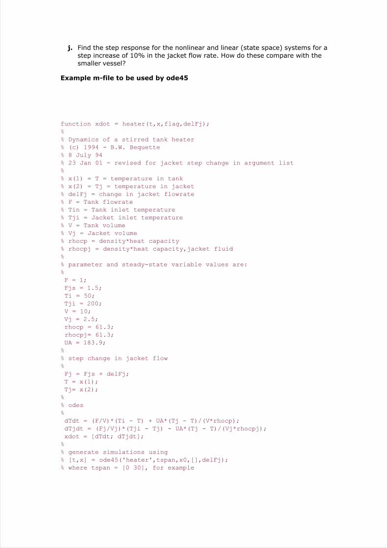
Example m-file to be used by ode45

function xdot = heater(t,x,flag,delFj);

%

% Dynamics of a stirred tank heater

% (c) 1994 - B.W. Bequette

% 8 July 94

% 23 Jan 01 - revised for jacket step change in argument list

%

% x(1) = T = temperature in tank

% x(2) = Tj = temperature in jacket

% delFj = change in jacket flowrate

% F = Tank flowrate

% Tin = Tank inlet temperature

% Tji = Jacket inlet temperature

% V = Tank volume

% Vj = Jacket volume

% rhocp = density*heat capacity

% rhocpj = density*heat capacity,jacket fluid

%

% parameter and steady-state variable values are:

%

F = 1;

Fjs = 1.5;

Ti = 50;

Tji = 200;

V = 10;

Vj = 2.5;

rhocp = 61.3;

rhocpj= 61.3;

UA = 183.9;

%

% step change in jacket flow

%

Fj = Fjs + delFj;

T = x(1);

Tj= x(2);

%

% odes

%

dTdt = (F/V)*(Ti - T) + UA*(Tj - T)/(V*rhocp);

dTjdt = (Fj/Vj)*(Tji - Tj) - UA*(Tj - T)/(Vj*rhocpj);

xdot = [dTdt; dTjdt];

%

% generate simulations using

% [t,x] = ode45('heater',tspan,x0,[],delFj);

% where tspan = [0 30], for example

To make the runs go faster, you may wish to generate and run the following script file:

%

% runs stirred tank heater example - 23 Jan 01

% step changes to stirred tank heater

%

% make certain you enter the step change value (delFj)

% before running this file

% also, generate function file with the following first line:

% function xdot = heater(t,x,flag,delFj);

%

options = odeset('RelTol',1e-6,'AbsTol',[1e-6 1e-6]);

%

[t,x] = ode45('heater',tspan,x0,options,delFj);

%

figure(1)

subplot(2,1,1),plot(t,x(:,1))

title('nonlinear, using ode45')

xlabel('time, min')

ylabel('temp, deg F')

subplot(2,1,2),plot(t,x(:,2))

xlabel('time, min')

ylabel('jacket temp, deg F')

%

% state space model with unit step change

a = [-0.4 0.3;1.2 -1.8];

b = [0;20];

c = [1 0;0 1];

d = 0;

sys = ss(a,b,c,d);

[ylin,tlin] = step(sys);

%

figure(2)

subplot(2,1,1),plot(tlin,ylin(:,1))

title('linear state space, unit step, deviation')

xlabel('time, min')

subplot(2,1,2),plot(tlin,ylin(:,2))

xlabel('time, min')

%

% scale deviation by delFj

ylinscale = ylin*delFj;

% plot in physical variable form

figure(3)

subplot(2,1,1),plot(tlin,125+ylinscale(:,1))

title('linear state space, physical magnitude')

xlabel('time, min')

subplot(2,1,2),plot(tlin,150+ylinscale(:,2))

xlabel('time, min')

% compare linear and nonlinear on same plot

figure(4)

subplot(2,1,1),plot(t,x(:,1),tlin,125+ylinscale(:,1),'--')

title('nonlinear vs. linear')

xlabel('time, min')

ylabel('temp, deg F')

legend('nonlinear','linear')

subplot(2,1,2),plot(t,x(:,2),tlin,150+ylinscale(:,2),'--')

xlabel('time, min')

ylabel('jacket temp, deg F')

legend('nonlinear','linear')

[ Team LiB ]

[ Team LiB ]

Appendix 2.1: Solving Algebraic Equations

Fortunately, the MATLAB fsolve function is easy to use for solving algebraic equations. For a

simplified presentation, we use the form

Equation A.1

obtained from Equation (2.66) with a fixed p and u. The most commonly used numericaltechniques are related to Newton-Raphson iteration. The "guess" for iteration k + 1 is determinedfrom the value at iteration k, using

Equation A.2

where f[x(k)] is the vector of function evaluations at iteration k, and J(k) is the Jacobian matrix

Equation A.3

The ij element of the Jacobian represents the partial derivative of equation i with respect tovariable j. If analytical derivatives are not available, elements of the Jacobian are obtained byperturbation of the state variable, requiring n + 1 function evaluations for an n-equation systemof equations. Various quasi-Newton techniques provide approximations to the Jacobian and do notrequire as many function evaluations, reducing computational time.

In practice, the Jacobian matrix in Equation (A.2) is not inverted. Rather, a set of linear algebraicequations is solved for x(k+1),

Equation A.4

In this text we do not focus on the solution of algebraic equations. See the text by Bequette(1998) for more details on these techniques.

[ Team LiB ]

[ Team LiB ]

Appendix 2.2: Integrating Ordinary Differential

Equations

The Euler integration method often requires very small integration step sizes to obtain a desiredlevel of accuracy. Note that x is a vector of n state variables at each time step. For example, ifthere are two states (two differential equations)

we have left the inputs and parameters out of the function variable list for convenience. Anexample is shown next.

Example 2.2: An Isothermal Chemical Reactor, continued

Consider the ethylene glycol reactor problem in Example 2.2. We use k1 to represent the reactionrate constant, so that it is not confused with the time-step index. The Euler integration algorithmresults in the following two equations, where k represents the time-step index.

For CA(0) = 0.1 and CP(0) = 0.4, and a space velocity (F/V) = 0.0816 min-1 we find, for the firsttime step,

Substituting the numerical values for an integration step size of 0.5 minutes, we find

resulting in the concentration values at t = 0.5 minutes

Values can be obtained at future times by continuing to march forward in time. MATLAB has a suiteof routines for integrating differential equations. These are covered in Module 3.

[ Team LiB ]

[ Team LiB ]

Chapter 3. Dynamic Behavior

The goal of this chapter is to understand dynamic behavior. We begin by working with linear statespace models, often obtained by linearizing a nonlinear model, such as those developed inChapter 2. We then introduce Laplace transforms. The main advantage to Laplace transforms isthat they allow us to analyze behavior exhibited by linear differential equations by using simplealgebraic manipulations. Laplace transforms are used to create transfer function models, whichare the basis for many control system design techniques.

After studying this chapter, the reader should be able to:

Apply the initial and final value theorems of Laplace transforms

Understand first-order, first-order + dead time and integrating system step responses

Understand second-order under-damped behavior

Understand the effect of pole and zero values on step responses

Convert state space models to transfer functions

The major sections of this chapter are as follows:

3.1 Background

3.2 Linear State Space Models

3.3 Introduction to Laplace Transforms

3.4 Transfer Functions

3.5 First-Order Behavior

3.6 Integrating System

3.7 Second-Order Behavior

3.8 Lead-Lag Behavior

3.9 Poles and Zeros

3.10 Processes with Dead Time

3.11 Padé Approximation for Dead Time

3.12 Converting State Space Models to Transfer Functions

3.13 MATLAB and SIMULINK

3.14 Summary

[ Team LiB ]

[ Team LiB ]

3.1 Background

One of the major goals of this chapter is to obtain an understanding of process dynamics. Processengineers tend to think of process dynamics in terms of the response of a process to a step inputchange. Assume that the process is initially at steady state, then apply a step change to an inputvariable. The majority of chemical processes will exhibit one of the responses shown in Figure 3-1. In this plot, we assume that a positive step increase has been made to the input variable ofinterest. The solid curves are examples of "positive gain" processes; that is, the process outputincreases for an increase in the input. The dashed lines are those of negative gain processes. Thecurves in Figure 3-1a show a monotonic change in the output; this behavior is generally known asoverdamped. The curves in Figure 3-1b are indicative of "integrating" processes; a prime exampleis a liquid surge vessel, where the level continues to change when there is an imbalance in theinlet and outlet flow rates. The curves in Figure 3-1c are known as underdamped or oscillatoryresponses. This type of behavior may occur in exothermic chemical reactors or biochemicalreactors. It more often occurs in processes that are under feedback control, particularly if thecontroller is poorly tuned. The behavior shown in Figure 3-1d is known as "inverse response" andis seen in steam drums, distillation columns, and some adiabatic plug flow reactors.

Figure 3-1. Common responses of process outputs to step changes inprocess inputs. Assuming a positive step change, the solid curves areillustrative of "positive gain" processes, and the dashed curves are

indicative of "negative gain" processes. (a) Overdamped or first order,(b) integrating, (c) underdamped or oscillatory, and (d) inverse

response.

In the sections that follow, we discuss the characteristics of process models that lead to each ofthe behaviors shown in Figure 3-1.

[ Team LiB ]

[ Team LiB ]

3.2 Linear State Space Models

In Chapter 2 we developed fundamental models, which were normally nonlinear in nature. Wethen developed state space models that were based on linearizing the fundamental models at asteady-state solution. This led to the notion of a perturbation or deviation variable, which issimply the perturbation of a variable from its steady-state value.

State space models have the following form, where the states (x), inputs (u), and outputs (y) areall perturbation or deviation variables

Equation 3.1

Recall that in matrix notation, the first subscript refers to the row and the second subscript refersto the column. When matrices multiply vectors, each row corresponds to a particular output of themultiplication, while the column corresponds to a particular input of the operation. Consider the Cmatrix, which relates the states to the outputs. Element cij relates the effect of state xj on outputyi.

The shorthand notation for Equation (3.1) is

Equation 3.2

It is important to always check for dimensional consistency in matrix operations. In a matrix-vector operation y = Cx, the number of rows in C must be equal to the number of elements in y.Also, the number of columns in C must be equal to the number of elements in x.

Stability

One of the first basic concepts that we need to cover is the notion of stability. Consider a processwhere one or more states have been perturbed from the steady-state solution or operating point.The process is stable if after a period of time, the variables return to the steady-state values. Thismeans that the state variables, since they are deviation variables, return to zero.

Numerically, we can determine the stability of a state space model by finding the eigenvalues of

the state space A matrix. Remember that the A matrix is simply the matrix of derivatives of thedynamic modeling equations with respect to the state variables.

If all of the eigenvalues are negative, then the system is stable; if any single eigenvalue ispositive, the system is unstable. A system with all but one eigenvalues negative and with oneeigenvalue equal to zero is called an integrating system and is characteristic of processes withliquid levels or gas drum pressures that can vary.

Examples of unstable systems are shown in Figure 3-2. If an eigenvalue is real and positive, thesystem response is that shown in the top curves. If there are complex conjugate eigenvalues,with positive real portions, the system oscillates (with ever increasing amplitude), as shown at thebottom.

Figure 3-2. Unstable responses. (a) Monotonic and (b) oscillatory.

Mathematically, the eigenvalues of the A matrix are found from the roots of the characteristic

polynomial

Equation 3.3

where λ is known as an eigenvalue, and I is the identity matrix. For a state space model with nstates, A is an n x n matrix, and there will be n solutions (eigenvalues) of Equation (3.3). Thereare analytical solutions for two- and three-state systems; the two-state solution is shown below.

In two-state systems,

The determinant can be found by

and the eigenvalues are found as the two solutions (roots) to

Equation 3.4

The roots can be found using the quadratic formula

Equation 3.5

It is easy to show that if and a11 + a22 < 0 and a11a22 >a12a21, the roots (eigenvalues) arenegative and the system is stable. A more general method of qualitatively checking the stability,known as the Routh stability criterion, is shown in Chapter 5.

Example 3.1: Exothermic CSTR

Models for an exothermic, CSTR are detailed in Module 8. For a two-state representation, the firststate is the concentration and the second state is the reactor temperature. For a particularreactor with two different operating conditions, the A matrix is (the time unit is hours)

Operating condition 1 Operating condition 2

and the eigenvalues for operating condition 1 can be found using the following steps

with the solutions [using the quadratic formula (3.5)]

Since both eigenvalues are negative, operating condition 1 is stable.

The reader should show that the eigenvalues of A2 are

where the positive eigenvalue indicates that operating condition 2 is unstable.

MATLAB Eigenvalue Function

The MATLAB eig command can be used to quickly find eigenvalues of a matrix. The reader should

use the MATLAB command window to verify the following results for the second operatingcondition:

» a2 = [-1.8124 -0.2324;9.6837 1.4697];

» eig(a2)

ans =

-0.8366

0.4939

Again, the positive eigenvalue indicates that the second operating condition is unstable.

Generalization

Notice that a solution of a second-order polynomial was required to find the eigenvalues of thetwo-state example; this resulted in two eigenvalues. For the general case of an n x n matrix,there will be n eigenvalues. It is too complex to find these analytically for all but the simplest low-order systems. The simplest way to find eigenvalues is by using existing numerical analysissoftware; for example, in MATLAB the eig function can be used to find eigenvalues.

The values of the eigenvalues are related to the "speed of response," and the eigenvalue unit isinverse time. If the unit of time used in the differential equations is minutes, for example, thenthe eigenvalues have min-1 as the unit. For stable systems (where all eigenvalues are negative),the larger magnitude (more negative) eigenvalues are faster.

For matrices that are 2 x 2 or larger, some eigenvalues may occur in complex conjugate pairs. Inthis case, the stability is determined by the sign of the real portion of the complex number. Aslong as all real portions are negative, the system is stable.

[ Team LiB ]

[ Team LiB ]

3.3 Introduction to Laplace Transforms

Most control system analysis and design techniques are based on linear systems theory. Althoughwe could develop these procedures using the state space models, it is generally easier to workwith transfer functions. Basically, transfer functions allow us to make algebraic manipulationsrather than working directly with linear differential equations (state space models). To createtransfer functions, we need the notion of the Laplace transform.

The Laplace transform of a time-domain function, f(t), is represented by L[f(t)] and is defined as

Equation 3.6

The Laplace transform is a linear operation, so the Laplace transform of a constant (C) multiplyinga time-domain function is just that constant times the Laplace transform of the function,

Equation 3.7

The Laplace transforms of a few common time-domain functions are shown next.

Exponential Function

Exponential functions appear often in the solution of linear differential equations. Here

The transform is defined for t > 0 (we also use the identity that ex+y = exey)

So we now have the following relationship:

Equation 3.8

Derivatives

This will be important in transforming the derivative term in a dynamic equation to the Laplacedomain (using integration by parts),

so we can write

Equation 3.9

For an nth derivative, we can derive

Equation 3.10

n initial conditions are needed: f(0),..., f(n – 1) (0)

One reason for using deviation variables is that all of the initial condition terms in Equation (3.10)are 0, if the system is initially at steady-state.

Time Delays (Dead Time)

Time delays often occur owing to fluid transport through pipes, or measurement sample delays.Here we use θ to represent the time delay. If f(t) represents a particular function of time, then f(t– θ) represents the value of the function θ time units in the past.

We can use a change of variables, t* = t – θ, to integrate the function. Notice that the lower limitof integration does not change, because the function is defined as f(t) = 0 for t < 0.

Equation 3.11

So the Laplace transform of a function with a time delay (θ) is simply e–θs times the Laplacetransform of the nondelayed function.

Step Functions

Step functions are used to simulate the sudden change in an input variable (say a flow rate beingrapidly changed from one value to another). A step function is discontinuous at t = 0. A "unit"step function is defined as

and using the definition of the Laplace transform,

so

Equation 3.12

Similarly, the Laplace transform of a constant, C, is

Equation 3.13

Pulse

Consider a pulse function, where a total integrated input of magnitude P is applied over tp timeunits, as shown in Figure 3-3.

Figure 3-3. Pulse function.

The function is f(t) = P/tp for 0 < t < tp and f(t) = 0 for t > tp. The Laplace transform is

Equation 3.14

Impulse

An impulse function can viewed as a pulse function, where the pulse period is decreased whilemaintaining the pulse area, as shown in Figure 3-4. In the limit, as tp approaches 0, the pulsefunction becomes (using L'Hopital's rule)

Equation 3.15

Figure 3-4. Concept of an impulse function.

If we denote a unit impulse as f(t) = δ, then the Laplace transform is

Equation 3.16

Examples of common impulse inputs include a "bolus" (shot or injection) of a drug into aphysiological system, or dumping a bucket of fluid or bag of solids into a chemical reactor.

Other Functions

It is rare for one to derive the Laplace transform for a function; rather a table of knowntransforms (and inverse transforms) can be used to solve most dynamic systems problems.

Table 3-1 presents solutions for most common functions. If you desire to transform a functionfrom the time domain to the Laplace domain, then look for the time-domain function in the firstcolumn and write the corresponding Laplace domain function from the second column. Similarly, ifyour goal is to "invert" a Laplace domain function to the time domain, then look for the Laplacedomain function in the second column and write the corresponding time-domain function from thefirst column. This notion of the inverse Laplace transform can be written

Equation 3.17

For example

Initial- and Final-Value Theorems

The following theorems are very useful for determining limiting values in dynamics and controlstudies. The long-term behavior of a time-domain function can be found by analyzing the Laplacedomain behavior in the limit as the s variable approaches zero. The initial value of a time-domainfunction can be found by analyzing the Laplace domain behavior in the limit as s approachesinfinity.

Table 3-1. Laplace Transforms for Common Time-Domain Functions

Time-domain function Laplace domain function

f(t) F(s)

δ(t) (unit impulse) 1

C (constant)

f(t - θ) e-θsF(s)

t

tn

sF(S) - f(0)

Snf(S) - Sn-1f(0) - L - sf(n-2)(0) - f(n-1)(0)

e-at

te-at

1-e-t/τ

sin ωt

Time-domain function Laplace domain function

cos ωt

e–at sin ωt

e–atcos ωt

where ,

The final-value theorem is

Equation 3.18a

The initial-value theorem is

Equation 3.18b

It should be noted that these theorems only hold for stable systems.

Example 3.2: Application of Initial- and Final-Value Theorems

Find the long-term and short-term behavior of the time-domain function, y(t), using the final- andinitial-value theorems on the Laplace domain function Y(s) (we see later that this arises from astep input applied to a second-order process):

The long-term behavior, y(t ), is found using the final-value theorem,

The short-term behavior, y(t 0), is found using the initial-value theorem,

The reader should verify that the time-domain function, y(t), can be found by applying Table 3-1to find

and that the values of y(t ), and y(t 0), are consistent with the final- and initial-valuetheorems.

General Solution Procedure

To obtain analytical solutions for differential equation-based models, the general procedure iscomposed of several steps.

Start with an nth order linear differential equation

and known initial conditions

1.

Transform each element of the differential equation to the Laplace domain,2.

Use algebraic manipulations to solve for the transformed variable.

where N(s) and D(s) are polynomials in s.

3.

Perform a partial fraction expansion to isolate the individual elements.

where a, b, and so forth are the roots of D(s). If roots are repeated the partial fractionexpansion has the form (for an example where three roots all have a value of a).

4.

Invert each element back to the time domain to find the final solution for y(t).

For the case of repeated roots (say 3 that have a value of a), the solution has the form

5.

It should be noted that chemical process systems are rarely described by an nth order differentialequation. Usually, a set of n first-order differential equations is transformed to a single nth orderequation, as shown in Example 3.3.

Example 3.3: Second-Order Differential Equation

Consider the following state space model of an isothermal CSTR (Module 5).

Equation 3.19

where x1 and x2 represent the concentrations of two components (in deviation variable form) inan isothermal reactor; the initial conditions are x1(0) = x2(0) = 0. Solve for the output(concentration of component 2) response to a unit step input.

The reader should show (see exercise 6) that this can be arranged to a second-orderdifferential equation,

with the initial conditions y(0) = dy(0)/dt = 0, and the input is initially u(0)= 0.

1.

Taking the Laplace transform of each element,

and substituting back into the differential equation, we find[1]

[1] Alternatively, one could take the Laplace transform of each equation in (3.19) and use algebraicsubstitution to find this second-order equation in s.

2.

Solving for Y(s), we find

Here we consider a unit step input, U(s) = 1/s.

3.

Performing a partial fraction expansion using the roots of the denominator polynomial,

Equation 3.20

4.

Solve for C1 by multiplying by s,

Setting s = 0 to find

Similarly, solve for C2 by multiplying Equation (3.20) by s + 2.4053 and setting s = –2.4053

Also, solve for C3 by multiplying Equation (3.20) by s + 2.2376 and setting s = –2.2376

which yields

Inverting each element back to the time domain,

Equation 3.21

Although it is nice to have an analytical solution, it is generally more pleasing to engineers toview a plot of a variable as it changes with time, as shown in Figure 3-5. In this plot wenotice that the concentration initially decreases, before increasing to a new steady-statevalue.

Figure 3-5. Response of the concentration as a function of time.See Equation (3.21).

5.

In Example 3.3 we solved for the coefficients (C1, C2, C3) by selecting values of s to minimize themultiplications performed during each step. An alternative is to solve for three equations in threeunknowns by using various values of s (say s = 1, 2, and 3, for example) in Equation (3.20).

Differential equations textbooks, such as Boyce and DiPrima (1992) present many examples ofapplications of Laplace transforms to solve differential equations. In practice, it is rare for processengineers to seek analytical solutions to differential equations; it is far easier to solve thesenumerically. The primary goal of this section was to provide background material to understandthe transfer functions and dynamic responses shown in the next section.

[ Team LiB ]

[ Team LiB ]

3.4 Transfer Functions

A transfer function relates inputs to outputs in the Laplace domain. In particular, the Laplacedomain relationship between a manipulated input and output is called a process transfer function.

Consider an nth order differential equation,

Equation 3.22a

Since we are assuming that the model is based on deviation variables, and that the system isinitially at steady state, the initial conditions are

Equation 3.22b

Taking the Laplace transform of each term,

Solving for Y(s), we find

The ratio of polynomials is called the transfer function. When it relates a manipulated input to anoutput it is commonly called a process transfer function. In general, we will use gp(s) to representthe process transfer function.

Equation 3.23

In this case the process transfer function is

Equation 3.24

The roots of the numerator polynomial are known as zeros, and the roots of the denominatorpolynomial are call poles. The significance of poles and zeros are discussed in detail in Section3.9.

We have used capital letters to distinguish Laplace domain variables from the time-domainvariables. In the rest of this text we generally use lowercase letters for all input and output

variables. If the argument is s, then we assume that we are referring to the Laplace domain.

Transfer functions are often used in block diagrams. For example, the relationship between aninput and output is shown as

In the rest of this chapter we study the dynamic behavior of some commonly used transferfunctions. Our focus is on Step Responses, since process engineers often apply step changes tounderstand dynamic behavior.

[ Team LiB ]

[ Team LiB ]

3.5 First-Order Behavior

Many chemical processes can be modeled as first-order systems. The differential equation for alinear first-order process is often written in the following form:

Equation 3.25

This can also be written as

where the parameters (τp and kp) and variables (y and u) have the following names: τp is theprocess time constant (units of time), kp the process gain (units of output/input), y the outputvariable, and u the input variable. Taking the Laplace transform of each term (notice that we are

now using lower-case variables to represent the Laplace domain input and output), and assumingthat the initial condition is y(0) = 0,

So the Laplace transform of Equation (3.25) can be written

or solving for y(s) we find a first-order transfer function

Equation 3.26

Step Response

Consider the case where the output is initially zero (steady state in deviation variable form), andthe input is suddenly step changed by an amount ∆u. The Laplace transform of the input is

Equation 3.27

So Equation (3.26) can be written

Equation 3.28

Using a partial fraction expansion and inverting to the time domain, you should find (see Exercise1)

Equation 3.29

Here the notion of a process gain is clear. After a substantial amount of time (t >> τp), we find,from Equation (3.29),

Equation 3.30

That is,

and, since y(0) = 0, we can think of y(t ) as ∆y, so

Equation 3.31

We can think of the process time constant as the amount of time it takes for 63.2% of theultimate output change to occur, since when t = τp,

Remember that this holds true only for first-order systems.

Impulse Response

Consider now an impulse input of magnitude P, which has units of the input*time; if the input is avolumetric flow rate (volume/time), then the impulse input is a volume. The output response is

You should find that the time domain solution is

which has an immediate response of Pkp/τp followed by a first-order decay with time.

Example 3.4: Stirred-Tank Heater

Recall that an energy balance on a constant-volume stirred-tank heater (Example 2.3) yielded

where the subscript s is used to indicate that a particular variable remains at its steady-statevalue. Defining the following deviation variables

The equation can be written in the form

or

where the parameters of this first-order model are

The gain and time constant are clearly a function of scale. A process with a large steady-stateflow rate will have a low gain, compared to a process with a small steady-state flow rate. Thismakes physical sense, since a given heat power input will have a larger effect on the smallprocess than the large process. Similarly, a process with a large volume-to-flow rate ratio isexpected to have a slow response compared to a process with a small volume-to-flow rate ratio.

Consider a heater with a constant liquid volume of Vs = 50 liters and a constant volumetric flowrate of Fs = 10 liters/minute. For liquid water, the other parameters are ρcp = 1 kcal/ liter°C. Theprocess gain and time constant are then

Step Response

If a step input change of 10 kW is made, the resulting output change is [from Equation (3.29)]

A plot of the step input and the resulting output are shown in Figure 3-6.

Figure 3-6. Step response of a stirred-tank heater, characteristic of afirst-order system. Deviation variables.

Remember that the inputs and outputs in this expression are in deviation variable form. If thesteady-state values are (for an inlet temperature of 20°C)

Then, the physical temperature response is

Impulse Response

If an impulse input of 30 kJ is made, you should be able to show that the temperature changesimmediately by 0.143°C (see Exercise 15).

[ Team LiB ]

[ Team LiB ]

3.6 Integrating System

We found in the previous chapter that material balances on liquid surge vessels or gas drumsoften yielded models with the following form:

Equation 3.32

In the Laplace domain, this is

Equation 3.33

Consider an integrating process initially at steady state, with y(0) = 0.

Step Response

If a step input change of ∆u is made at t = 0,

and we find the time-domain value

Equation 3.34

That is, the output ramps with a constant slope of k∆u.

Impulse Response

If an impulse input of magnitude P is made at t = 0,

then the output immediately changes to a new steady-state value of

Example 3.5: Tank-Height Problem

The mathematical model for a liquid surge tank is (see Example 1.3)

where h is the liquid height, A is the constant cross-sectional area of the tank, F1 is the inlet flowrate, and F2 is the outlet flow rate. Assume that the outlet flow rate remains constant at a steady-state value of F2s. Defining the output and input in deviation variable form as

For a constant cross-sectional area of 10 m2, the model is

Step Response

For a step input change of 0.25 m3/min, the output response is

which is shown in Figure 3-7. If the steady-state height is 2 meters, then the height as a functionof time is

Figure 3-7. Step response of a liquid surge tank. Deviation variables.

Impulse Response

For an impulse input of 1 m3, the output response is

which makes sense, because the cross-sectional area is 10 m3.

[ Team LiB ]

[ Team LiB ]

3.7 Second-Order Behavior

Second-order models arise from systems that are modeled with two differential equations (twostates). In this section we separately consider transfer functions that do not have "numerator"dynamics and those that do.

Pure Second-Order Systems

Consider a linear second-order ODE, with constant parameters

Equation 3.35

This is often written in the form

Equation 3.36

where (obviously a0 0)

and the parameters are as follows: k is the gain (units of output/input), ζ the damping factor(dimensionless), and τ the natural period (units of time).

The second-order model shown in Equation (3.35) or (3.36) generally arises by changing a set oftwo first-order equations (state-space model) to a single second-order equation. For a givensecond-order ODE, there are an infinite number of sets of two first-order (state-space) modelsthat are equivalent.

Taking the Laplace transform of Equation (3.36),

Equation 3.37

where y(s) indicates the Laplace transformed variable.

Assuming initial conditions are zero, that is , we find

Equation 3.38

The characteristic equation of the second-order transfer function is τ2s2 + 2ζτs + 1. We can findthe roots (known as the poles) by using the quadratic formula

which yields the following values for the roots:

Equation 3.39

The following analysis assumes that ζ >0 and τ > 0. This implies that the real portions of p1 andp2 are negative and, therefore, the system is stable. The three possible cases are shown in Table3-2.

Step Responses

Now, we consider the dynamic response of second-order systems to step inputs (u(s) = ∆u/s),

Equation 3.40

where ∆u represents the magnitude of the step change.

Case 1: Overdamped (• > 1)

For ζ > 1, the denominator polynomial, τ2s2 + 2ζτs + 1, can be factored into the form

where the time constants are

Table 3-2. Characteristic Behavior of Second-Order Transfer Functions

Case Damping factor Pole location Characteristic behavior

1 ζ > 1 Two real, distinct roots Overdamped

2 ζ = 1 Two real, equal roots Critically damped

3 ζ < 1 Two complex conjugate roots Underdamped

We can derive the following solution for step responses of overdamped systems,

Equation 3.41

Note that, as in the case of first-order systems, we can divide by k∆u to develop a dimensionlessoutput. Also, the dimensionless time is t/τ and we can plot curves for dimensionless output as afunction of ζ. This is done in Figure 3-8, which includes the critically damped case, as discussednext. Most chemical processes exhibit overdamped behavior.

Figure 3-8. Step response of a second-order overdamped system.

Case 2: Critically damped (• = 1)

The transition between overdamped and under damped is known as critically damped. We canderive the following for the step response of a critically damped system

Equation 3.42

Notice that the main difference between overdamped (or critically damped) step responses andfirst-order step responses is that the second-order step responses have an S shape with amaximum slope at an inflection point, whereas the first-order responses have their maximumslope initially.

The initial behavior for a step change is really dictated by the relative order of the system. Therelative order is the difference between the orders of the numerator and denominator polynomialsin the transfer function. If the relative order is 1, then output response has a nonzero slope at thetime of the step input; the step response of a system with a relative order greater than 1 has azero slope at the time of the step input.

Case 3: Underdamped (• < 1)

For ζ < 1, we find [from Equation (3.39)] that the poles are complex,

Equation 3.43a

where the real and imaginary contributions are

Equation 3.43b

We can derive the following step response for an underdamped system,

Equation 3.44a

where

Equation 3.44b

Again, dividing Equation (3.44a) by k∆u, we can produce the dimensionless plot shown in Figure3-9.

Figure 3-9. Step response of a second-order underdamped system as afunction of the damping factor (•). Interpolate between the curves for

the behavior of other damping factor values.

A number of insights can be obtained from Figure 3-9 and from an analysis of the step responseequations. For ζ < 1, the ratio of the imaginary portion to the real portion of the pole [fromEquation (3.39)] is

As the imaginary/real ratio gets larger, the response becomes more oscillatory (ζ becomessmaller). We also notice that a decreasing ratio corresponds to a larger negative value for the realportion. As the real portion becomes larger in magnitude (more negative), the response becomesfaster. We use these insights to interpret pole/zero plots in Section 3.9.

Underdamped Step Response Characteristics

The following common measures of underdamped second-order step responses are shown inFigure 3-10, and defined below: (1) rise time, (2) time to first peak, (3) overshoot, (4) decayratio, and (5) period of oscillation.

Figure 3-10. Step response characteristics of underdamped second-order processes.

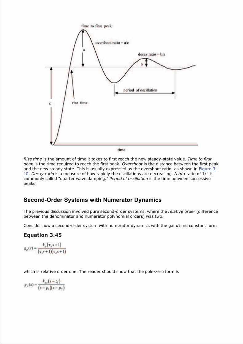
Rise time is the amount of time it takes to first reach the new steady-state value. Time to first

peak is the time required to reach the first peak. Overshoot is the distance between the first peakand the new steady state. This is usually expressed as the overshoot ratio, as shown in Figure 3-10. Decay ratio is a measure of how rapidly the oscillations are decreasing. A b/a ratio of 1/4 iscommonly called "quarter wave damping." Period of oscillation is the time between successivepeaks.

Second-Order Systems with Numerator Dynamics

The previous discussion involved pure second-order systems, where the relative order (differencebetween the denominator and numerator polynomial orders) was two.

Consider now a second-order system with numerator dynamics with the gain/time constant form

Equation 3.45

which is relative order one. The reader should show that the pole-zero form is

where the parameters are

The gain/time constant form has the following time-domain response to a step input (see Exercise4):

Equation 3.46

The reader should show that, if τn = τ2, the response is the same as a first-order process.

Example 3.6: Illustration of Numerator Dynamics

Consider the following input-output relationship:

The unit step responses are shown in Figure 3-11. Notice that negative numerator time constants(corresponding to positive zeros) yield a step response which initially decreases before increasingto the final steady state. This type of response is known as inverse response and causes toughchallenges for process control systems. Positive zeros are often caused by two first-order transferfunctions, with gains of opposite sign, acting in parallel (see Exercise 5).

Figure 3-11. Step responses of a second-order system with numeratordynamics.

Notice also that a numerator time constant that is greater than the denominator time constantcauses overshoot before settling to the final steady state. Also notice that the inverse responsebecomes "deeper" as the numerator zero (–1/τn) approaches a value of 0 from the positive side.

[ Team LiB ]

[ Team LiB ]

3.8 Lead-Lag Behavior

Lead-lag transfer functions have the same order numerator polynomial as denominatorpolynomial. This occurs when the input has a direct effect on the output variable. In terms of the

state space model (3.2), this means that D 0.

Consider a lead-lag transfer function where the numerator and denominator polynomials are firstorder:

Equation 3.47

For a step input of magnitude ∆u, the output response is

Equation 3.48

A dimensionless output can be defined by dividing Equation (3.48) by kp∆u, and t/τp is a naturaldimensionless time. The responses to a step input at t = 0 are shown in Figure 3-12. Notice thatthere is an immediate response that is equal to the τn/τp ratio. This can also be found by applyingthe initial value theorem to Equation (3.47"/>) for a step input change (see Exercise 3).

Figure 3-12. Step responses of the lead-lag example.

It is rare for processes to exhibit lead-lag behavior, but many controllers exhibit such behavior.

[ Team LiB ]

[ Team LiB ]

3.9 Poles and Zeros

There are a number of different ways to represent process transfer functions. The "polynomial"form is

Equation 3.49

The values of s that cause the numerator of Equation (3.49) to equal zero are known as the"zeros" of the transfer function. The values of s that cause the denominator of Equation (3.49) toequal zero are known as the "poles" of the transfer function.

The "pole-zero" form is

Equation 3.50

and complex poles (or zeros) must occur in complex conjugate pairs.

The "gain-time constant" form is the one that we use most often for control system design.

Equation 3.51

where τni is a numerator time constant and τpi is a denominator time constant. This form isnormally used when the roots (poles) of the denominator polynomial are real.

Example 3.7: Comparison of Various Transfer Function Forms

Consider a transfer function with the following gain-time constant form

The polynomial form is

The gain-polynomial form is

and the pole-zero form is

The zero is 1/10, and the poles are –1/3 and –1/15.

Notice that the zero for Example 3.7 is positive. A positive zero is called a right-half-plane (RHP)zero, because it appears in the right half of the complex plane (with real and imaginary axes).RHP zeros have a characteristic inverse response, as shown in Figure 3-11 for τn = -10 (whichcorresponds to a zero of +0.1).

Also notice that the poles are negative (left-half-plane), indicating a stable process. RHP (positive)poles are unstable. Recall that complex poles will yield an oscillatory response. A pole-zero plot ofthe transfer function in Example 3.7 is shown in Figure 3-13 [the pole locations are (-1/3,0) and(-1/15,0) and the zero location is (1/10,0), with the coordinates (real,imaginary)]. For thissystem, there is no imaginary component and the poles and zeros lie on the real axis.

Figure 3-13. Pole-zero location plot for Example 3.7 (x, poles; o, zero).

As poles move further to the left they yield a faster response, and increasing the magnitude of theimaginary portion makes the response more oscillatory. This behavior is summarized in Figure 3-14. Recall also that a process with a pole at the origin (and none in the RHP) is known as anintegrating system; that is, the system never settles to a steady state when a step input change

is made.

Figure 3-14. Effect of pole-zero location on dynamic behavior (x,poles; o, zero). As poles become more negative, the response is faster.

As the imaginary/real ratio increases, the response becomes moreoscillatory.

Multiple RHP zeros cause multiple "changes in direction"; for example, with two RHP zeros, thestep response, initially going in one direction, switches direction, then switches back to the initialdirection.

[ Team LiB ]

[ Team LiB ]

3.10 Processes with Dead Time

Many processes have a delayed response to a process input, either due to transport lags (such asflow through pipes) or high-order effects. In Section 3.3.4 we found that a time-delay of θ timeunits had a transfer function of e–θs.

A first-order process combined with a time-delay has the transfer function

Consider a process with kp = 1, τp = 10, and θ = 5. A unit step input change at t = 0 yields theresponse shown in Figure 3-15. We see that the time-delay shifts the response of the output.

Figure 3-15. Response of a first-order + dead time process.

[ Team LiB ]

[ Team LiB ]

3.11 Padé Approximation for Dead Time

As discussed in the previous section the transfer function for a pure time delay is e–θs, where θ isthe time delay. Some control system design techniques require a rational transfer function; thePadé approximation for dead time is often used in this case.

A first-order Padé approximation is

A second-order Padé approximation is

Example 3.8: Application of the Padé Approximations for Dead Time

Consider the first-order + dead time transfer function, where the time-delay dominates the timeconstant

The first-order Padé approximation yields the transfer function

and the second-order Padé approximation yields

A comparison of the step responses of g(s), g1(s), and g2(s) is shown in Figure 3-16. Notice thatthe first-order approximation has an inverse response, while the second-order approximation hasa "double inverse response." The reader should find that there is a single positive zero for g1(s),and there are two positive, complex-conjugate zeros of the numerator transfer function of g2(s).

Figure 3-16. Comparison of first-order + dead time response with firstand second-order Padé approximations for dead time.

Most ordinary differential equation numerical integrators require pure differential equations (withno time delays). If you have a system of differential equations that has time delays, the Padéapproximation can be used to convert them to delay-free differential equations, which can then benumerically integrated.

One of the many advantages to using SIMULINK is that time delays are easily handled so that noapproximation is required.

[ Team LiB ]

[ Team LiB ]

3.12 Converting State Space Models to Transfer

Functions

A general state space model can be converted to transfer function form, using the following steps.Starting with the state space model

Take the Laplace transform of each term, assuming zero initial conditions

Solving for x(s), then y(s) (it should be noted that often D = 0)

where G(s) is a transfer function matrix. For example, the transfer function relating input j andoutput i is

or in matrix form (with m inputs and r outputs)

Example 3.9: Isothermal CSTR

Consider the isothermal CSTR shown in Example 3.3 and Module 5. The state space model is

The first input (u1, manipulated) is the dilution rate (F/V), the second input (u2, disturbance) isthe feed concentration (CAf), and the output is the concentration of the intermediate component,B. The eigenvalues of A (obtained by solving det(λI – A) = 0) are –2.4048 and –2.2381 min-1.

The sequence of steps used to find the transfer function matrix is

and multiplying,

Also,

The manipulated input-output process transfer function for the reactor is

and the disturbance input-output transfer function is

The transfer function poles (–2.2381 and –2.4048) are equal to the eigenvalues of the A matrix.Also, the positive zero (1/0.3549) in g11(s) yields the inverse response shown in Figure 3-5.

We see that it is straightforward to convert state space models to transfer function models. An n-state system results in transfer functions that have a denominator polynomial that is nth order ins, that is, with n poles. Sometimes the resulting transfer functions can be factored into lowerorder transfer functions because of pole-zero cancellation (a value of a pole is equal to a value ofa zero). An example of pole-zero cancellation is shown in Exercise 13.

[ Team LiB ]

[ Team LiB ]

3.13 MATLAB and SIMULINK

MATLAB and SIMULINK are ideal for analyzing and simulating dynamic behavior. The Control Toolboxuses LTI (linear, time invariant) objects to represent dynamic models. These objects can be statespace or transfer function models; details on how to use these are presented in Module 4.

Here we first present some useful MATLAB functions not covered in other modules.

conv (Convolution) and roots

Often it is necessary to multiply polynomials in s together. Although the following multiplication isquite simple: (5s + 1)(3s + 1) = 15s2 + 8s + 1, a more complex multiplication, such as (2s2 +1.5s + 1)(3s3 + 8s2 + 4s + 1) could be quite time consuming. The following conv (convolve)

command makes this straightforward. Also, the roots of the resulting polynomial are easilycalculated using the roots command.

» g = conv([2 1.5 1],[3 8 4 1])

g =

6.0000 20.5000 23.0000 16.0000 5.5000 1.0000

» p = roots(g)

p =

-2.1095

-0.3750 + 0.5995i

-0.3750 - 0.5995i

-0.2786 + 0.2836i

-0.2786 - 0.2836i

step

First, define an object, such one of the transfer functions in Example 3.6.

» num = [-10 1]; den = [45 18 1];

» sysc = tf(num,den)

Transfer function:

-10 s + 1

-----------------

45 s^2 + 18 s + 1

then plot the step response (use help step to view other options)

» step(sysc)

A number of other useful functions, such as pole and tzero are shown in Module 4.

Simulink

It is highly recommended that you interactively work through the initial sections of Module 2 tounderstand how SIMULINK can be used to simulate dynamic systems.

[ Team LiB ]

[ Team LiB ]

3.14 Summary

The main objective of this chapter was to develop an understanding of dynamic process behavior.Although Laplace transforms can be used to obtain analytical solutions to differential equations,we will not be using them for this purpose during the rest of this textbook. The concept of atransfer function is very useful for control system design and analysis. In future chapters we findthat transfer functions allow the use of algebra rather than differential equations when analyzingcontrol systems composed of a number of components (controller, valve, process, sensor, etc.).

The stability of a process is determined by the eigenvalues of the state space A matrix, or thepoles of the Laplace transfer function: if all are negative, the system is stable. Complexeigenvalues (poles) correspond to underdamped (oscillatory) behavior, characterized by dampingfactors less than 1. Dynamic responses are also affected by the values of the zeros (roots of thenumerator polynomial in s) of a transfer function. If zeros are positive (in the right-half-plane),step responses have a characteristic inverse response.

A first-order + dead time model is the most common process representation. Time-delays arerepresented by an irrational term (e–θs) in the Laplace domain. First and second-order Padéapproximations are sometimes used for controller design; the approximations lead to right-half-plane zeros and inverse response.

The initial and final value theorems of Laplace transforms can be used to find the limiting behaviorof transfer functions without having to obtain a full solution. The process gain is a measure of thelong-term change in a process output for a given input change.

State space models are easily converted to Laplace transfer function models. The use of LTIobjects (see Module 4) allows easy interconversion of models in MATLAB.

[ Team LiB ]

[ Team LiB ]

References

For more details on analytical mathematical methods (including Laplace transforms) to solvedifferential equations, see: Boyce, W., and R. DiPrima, Ordinary Differential Equations and

Boundary Value Problems, 5th ed., Wiley, New York (1992).

[ Team LiB ]

[ Team LiB ]

Student Exercises

1: Solve for the time-domain output of a first-order transfer function to a step inputchange.

2: A second-order process with one pole at the origin has the transfer function

Find the output as a function of time, for a unit step input change. Sketch the expectedbehavior.

3: Use the initial value theorem to find the immediate response of a lead-lag transferfunction to a step input change at t = 0.

Also, use the final value theorem to find the long-term response of a lead-lag transferfunction to a step input change.

4: For the following second-order process with numerator dynamics, solve for the time-domain output response to a step input change of magnitude ∆u at t =0.

For kp = 1°C/Lpm, τ1 = 3 min, τ2 = 15 min, τn = 20 min find the peak temperatureand the time that it occurs.

5: Consider an input-output transfer function that mimics two first-order processes inparallel

where

If the gain of g1 is positive and the gain of g2 is negative, find the conditions(relationship between gains and time constants for the two transfer functions) thatcause a right-half-plane zero (resulting in inverse response to a step input change) ingp(s).

6: Consider the state space model

Find the second-order differential equation in y. Hint: first solve for x1 from the secondequation, then take the derivative and substitute into the first equation.

7: Consider the following state-space model

Which has the following input-output transfer function relationship

For a unit step change in the input, u(s) = 1/s:

Find the output at t=0 and as t approaches infinity, using the initial and finalvalue theorems.

i.

Find the time domain solution, y(t)ii.

Sketch the time domain behavior of y(t)iii.

Are your results for i, ii, and iii consistent?iv.

8: As a process engineer with the Complex Pole Corporation, you are assigned a unit withan exothermic chemical reactor. In order to learn more about the dynamics of theprocess, you decide to make a step change in the input variable, the coolanttemperature, from 10°C to 15°C. Assume that the reactor was initially at a steadystate. You obtain the following plot for the output variable, which is reactortemperature (notice that the reactor temperature is in °F). Use Figure 3-9 to helpanswer the following questions.

What is the value of the process gain? (show units)i.

What is the value of τ? (show units)ii.

What is the value of ζ? (show units)iii.

What is the decay ratio?iv.

What is the period of oscillation? (show units)v.

Write the second-order transfer function.

Hint: Use Figure 3-9 to assist you.

vi.

9: Match the transfer functions with the responses to a unit step input, shown in thefigure.

i.

ii.

iii.

iv.

v.

10: Consider the following state space model:

Find the transfer function model.i.

Find (analytically) the time-domain output response to a unit step input change.Sketch the expected response to a unit step input change.

ii.

11: As a process engineer, you decide to develop a first-order + time delay model of aprocess using a step test. The process is initially at steady state, with an input flowrate of 5 gpm and an output of 0.75 mol/L. You make a step increase of 0.5 gpm at3:00 p.m. and do not observe any changes until 3:07 p.m. At 3:20 p.m., the value ofthe output is 0.8 mol/L. You become distracted and do not have a chance to look atthe output variable again, until you leave for happy hour at a local watering hole at6:30 p.m. You note that the output has ceased to change and has achieved a newsteady-state value of 0.85 mol/L. What are the values of the process parameters, withunits? Show your work.

12: Use the initial and final value theorems of Laplace transforms to determine the initialand final values of the process output for a unit step input change to the followingtransfer functions.

i.

ii.

iii.

13: Consider the following state space model for a biochemical reactor. Since there are twostates (the A matrix is 2 x 2) we expect that the process transfer function will besecond-order. Show that pole-zero cancellation occurs, resulting in a first-ordertransfer function. Find the values of the gain and time constant.

14: Match the transfer functions with the responses to a unit step input, shown in thefigure.

i.

ii.

iii.

iv.

v.

15: Consider Example 3.4. For an impulse input of 30 kJ, find the value of the vesseltemperature immediately after the impulse input is applied.

16: Consider the following second-order transfer function

For a unit impulse input, find the output response as a function of time. What is thepeak change and when does it occur?

[ Team LiB ]