Process and Measurement Noise Estimation for Kalman Filtering Yalcin Bulut1, D. Vines-Cavanaugh2, Dionisio Bernal3

Department of Civil and Environmental Engineering, 427 Snell Engineering Center

Northeastern University, Boston 02215, MA, USA

ybulut@coe.neu.edu, vines-cavanau.d@neu.edu, d.bernal@neu.edu 1 PhD Candidate, 2 PhD Student, 3 Associate Professor

ABSTRACT

The Kalman filter gain can be extracted from output signals but the covariance of the state error

cannot be evaluated without knowledge of the covariance of the process and measurement noise Q

and R. Among the methods that have been developed to estimate Q and R from measurements the

two that have received most attention are based on linear relations between these matrices and: 1)

the covariance function of the innovations from any stable filter or 2) the covariance function of the

output measurements. This paper reviews the two approaches and offers some observations

regarding how the initial estimate of the gain in the innovations approach may affect accuracy.

Keywords: Kalman Filter, Process Noise, Measurement Noise

NOMENCLATURE

A Discrete system matrix

B Input matrix of dynamic system

C Measurement matrix of state space model

E Expected value operator

K Steady state Kalman gain

0K Initial steady state Kalman gain

jl Estimate of the covariance function of the innovation process

jl Covariance function of the innovation process

Ob Observability matrix

0P Initial state error covariance matrix

P State error covariance matrix

0x Initial state vector

kx State vector at time k

ˆkx− State estimate after the measurement at time k is taken into consideration

ˆkx− State estimate before the measurement at time k is taken into consideration

Proceedings of the IMAC-XXVIIIFebruary 1–4, 2010, Jacksonville, Florida USA

©2010 Society for Experimental Mechanics Inc.

ky Discrete measurement vector

kw Discrete process noise

kv Discrete measurement noise

R Estimate of the covariance matrix of the measurement noise

R Covariance matrix of the measurement noise

Q Estimate of the covariance matrix of the process noise

Q Covariance matrix of the process noise

Σ State covariance matrix

jΛ Covariance function of the output

† Pseudo inverse matrix operator

INTRODUCTION

The basic idea in estimation theory is to obtain approximations of the true response by using

information from a model and from any available measurements. The mathematical structure used to

perform estimation is known as an observer. The optimal observer for linear systems subjected to

broad band disturbances is the Kalman Filter (KF). In the classical presentation of the filter the gain, K,

is computed given the model parameters and the covariance of the process and the measurement

noise, Q and R, respectively. Since Q and R are seldom known a priori work to determine how to

estimate these matrices from the measured data began soon after introduction of the filter. An

important result, apparently first published by Son and Anderson [1], is the fact that the information

needed to determine K is encoded in the output signals and thus, given sufficiently long data

sequences K can be estimated from the measurements without the need to know or estimate the Q, R

matrices. Perhaps the most widely quoted strategies to carry out the estimation of K are due to Mehra

[2] who built on the work by Heffes [3] and the subsequent paper by Carew and Bellanger [4], both

techniques being iterative in nature. A noteworthy contribution from this early work is the contributions

by Neethling and Young [5], who suggested some computational adjustments that could be used to

improve accuracy. The problem of computing K can be approached, of course, as one of estimating Q and R because

once these matrices are known K follows from well known relations. If all that is of interest is K,

therefore, one can take the direct approach, i.e., from the data to K, or the indirect one that estimates

Q and R first. Nevertheless, if in addition to estimating the state one is interested in the covariance of

the state error then the computation of Q and R becomes necessary since there is no direct approach

(at least not known to the writers) to go from the data to the state error covariance P. The two

approaches that have received most attention in the Q, R estimation problem are based on: 1)

correlations of the innovation sequence and 2) correlations of the output.

In the innovations approach one begins by “guessing” a filter gain (usually be estimating some Q

and R from whatever a priori knowledge there may be) and then the approach obtains the optimal

gain, the K, from analysis of the resulting innovations. In the limiting case where the output sequences

are very long (infinite in principle) the results converge to the exact solution independently of the initial

“guess”. In the real situation, however, where one must operates with finite length sequences (finite

precision and so on) the results for Q and R do depend on the initial estimation and a question that

arises is whether the answer is sensitive or not. . In this regard, Mehra [6] suggested that the

estimation of Q and R could be repeated by starting with the gain obtained in the first attempt but this

expectation was challenged by Carew and Bellanger [4], who noted that the exact gain is used as the

initial guess the approximations in the approach are such that the correctness will not be confirmed.

Some observations on the issue of the initial gain are presented later in this paper.

The output correlation approach can be viewed as a special case of the innovations where the

initial gain is taken as zero. In practice, however, the output correlation alternative has been discussed

as a separate approach (probably) because the mathematical arrangements that are possible in this

special case cannot be easily extended to the case where K ≠ 0. It is opportune to note that some

recent work on the estimation of Q and R has taken place in the structural health monitoring

community but the work appears to have been done in isolation of the classical works noted

previously, [7]. Part of the motivation for this paper is to offer a concise review of the classical

correlation based approaches that may prove useful in the structural engineering community. The

paper is organized as follows: the next section provides a brief summary of the KF particularized to a

time invariant linear system with stationary disturbances (which is a condition we have implicitly

assumed throughout the previous discussion). The following two sections review the formulations to

estimate Q and R using the innovations and output correlations and the paper concludes with a

numerical example.

THE KALMAN FILTER

Consider a time invariant linear system with unmeasured disturbances w(t) and available measurements y(t) that are linearly related to the state vector x(t). The system has the following description in sampled time

1k k kx Ax Bw+ = + (1)

k k ky Cx v= + (2) where nxn A∈ ,

nxr B∈ and mxn C∈ are the transition, input to state and state to output

matrices, mx1 ky ∈ is the measurement vector and nx1 kx ∈ is the state. The sequence nx1 kw ∈ is known as the process noise and mx1 kv ∈ is the measurement noise. In the

treatment here, it is assumed that these are uncorrelated Gaussian stationary white noise sequences

with zero mean and covariance of Q and R, namely

( 0 () )Tk k j kjw wE E w Qδ= = (3a,b)

( 0 () )Tk k j kjv vE E v Rδ= = (4a,b)

)( 0Tk jE v w = (5)

where kjδ denotes the Kronecker delta function and ( )Ε ⋅ denotes expectation. For the system in

eqs.1 and 2 the KF estimate of the state can be computed from

1ˆ ˆk kx Ax− ++ = (6)

ˆ ˆ ˆ( )k k k kx x K y Cx+ − −= + − (7) where kx

+ is the estimate after the information from the measurement at time k is taken into

consideration and ˆkx− is the estimate before. The (steady state) Kalman gain K can be expressed in a

number of alternative ways, a popular one is [8] 1( )T TK PC CPC R −= + (8) where P, the steady state covariance of the state error, is the solution of the Riccati equation 1( ( ) )T T T TP A P PC CPC R CP A BQB−= − + + (9)

The KF provides an estimate of the state for which P is minimal. The filter is initialized as follows

0 0ˆ [ ]x E x+ = (10)

0 0 0 0 0ˆ ˆ[( )( ) ]TP E x x x x= − − (11)

INNOVATIONS CORRELATION APPROACH FOR Q AND R ESTIMATION

We begin with the expression for the covariance function of the innovation process for any stable

observer with gain K0. As shown by Mehra [2] this function is

0Tjl CPC R j= + = (12)

10 0[ ( )] [ ( )] 0j T T

jl C A I K C A PC K CPC R j−= − − + > (13) where the covariance of the state error in the steady state, as shown by Heffes [3] is the solution of the

Riccati equation

0 0 0 0( ) ( )T T T T TP A I K C P I K C A AK RK A BQB= − − + + (14)

Estimation of PCT

Listing explicitly the covariance function for lags one to one has

1 0 0( )Tl CA PC K l= − (15)

2 0 0 0[ ( )] ( )Tl C A I K C A PC K l= − − (16)

23 0 0 0[ ( )] ( )Tl C A I K C A PC K l= − − (17)

..................... 1

0 0 0[ ( )] ( )Tl C A I K C A PC K l−= − − (18) from where one can write

0 0( )TL Z PC K l= − (19)

In which,

1

2 02

3 0

10

[ ( )] [ ( )]

... ......[ ( )]

l CAl C A I K C A

L l Z C A I K C A

l C A I K C A−

⎡ ⎤⎡ ⎤⎢ ⎥⎢ ⎥ −⎢ ⎥⎢ ⎥⎢ ⎥⎢ ⎥= = −⎢ ⎥⎢ ⎥⎢ ⎥⎢ ⎥⎢ ⎥⎢ ⎥ −⎣ ⎦ ⎣ ⎦

(20a,b)

As can be seen, matrix Z is the observability block of an observer whose gain is K0 post-multiplied by

the transition matrix A. On the assumption that the closed loop is stable and observable, one

concludes that Z attains full column rank when is no larger than the order of the system, n.

Accepting that the matrix is full rank one finds that the unique least square solution to eq.19 is

†0 0

TPC K l Z L= + (21)

where †Z is the pseudo-inverse of Z . On the premise that the model is known without error (which is a strong assumption), error in solving eq.21 for PCT results from the fact that the innovations

covariance is approximate due to the finite duration of the signals.

Estimation of R

Having obtained an estimate for PCT, the covariance of the output noise R can be estimated from

eq.12 as

0ˆˆ ˆ( )TR l C PC= − (22)

where the hats are added to emphasize that the quantities are estimates.

Estimation of Q

Derivation of an expression to estimate Q is significantly more involved than the one for R. The

process begins by replacing, in eq.14, the covariance R by its expression in terms of the

autocorrelation at zero lag. After some algebra one gets

T TP APA M BQB= + + (23) where

0 0 0 0 0[ ]T T T TM A K CP PC K K l K A= − − + (24)

Now consider a recursive solution for P in eq.23. In a first substitution one has ( )T T T TP A APA M BQB A M BQB= + + + + (25) or 2 2( )T T T T TP A P A AMA ABQB A M BQB= + + + + (26)

and after q substitutions one gets

1 1

0 0( ) ( ) ( )

q qq q T j j T j T j T

j jP A P A A M A A BQB A

− −

= =

= + +∑ ∑ (27)

Before solving eq.27 for Q it is first necessary to extract the set of equations for which only knowledge

of PCT (estimated by eq.21) is necessary. These equations are attained by post-multiplying both sides

of eq.27 by CT and pre-multiplying by CA-q. This gives

1 1

0 0( ) ( ) ( )

q qq T q T T q j j T T q j T j T T

j jCA PC CP A C CA A M A C CA A BQB A C

− −− − −

= =

= + +∑ ∑ (28)

Given that P is symmetric, the CP product to the right of the equal sign can be expressed as ( )T TPC ,

and one has

1 1

0 0( ) ( ) ( ) ( )

q qj q T j T T q T T T q T T j q j T T

j j

CA BQB A C CA PC PC A C CA M A C− −

− − −

= =

= − −∑ ∑ (29)

For convenience we transpose both sides of eq.29 and get

1 1

0 0( ) ( ) ( ) ( )

q qj T j q T T T T q T T q T j j q T T

j j

CA BQB A C PC A C CA PC CA M A C− −

− − −

= =

= − −∑ ∑ (30)

where we’ve accounted for the fact that M is symmetrical. To shorten eq.30 we define

jjF CA B= (31)

( )T j q T TjG B A C−= (32)

and

1

0( ) ( ) ( )

qT T q T T q T j j q T T

qj

s PC A C CA PC CA M A C−

− −

=

= − −∑ (33)

So eq.30 becomes

1

0

q

j j qj

F QG s−

=

=∑ (34)

Applying the vec operator to both sides of eq.34 one has

1

0

( ) ( ) ( )q

Tj j q

j

G F vec Q vec s−

=

⊗ ⋅ =∑ (35)

where⊗ denotes the Kronecker product. Eq.35 can be evaluated for as many q values as one desires,

although it is evident that all the equations obtained are not necessarily independent. Selecting q from

one to p gives ( )H vec Q S⋅ = (36) where

1 1

12 2

0

( )( )

( ) .. ..

( )

qT

q j jj

p p

h vec sh vec s

h G F H S

h vec s

−

=

⎡ ⎤ ⎡ ⎤⎢ ⎥ ⎢ ⎥⎢ ⎥ ⎢ ⎥= ⊗ = =⎢ ⎥ ⎢ ⎥⎢ ⎥ ⎢ ⎥⎢ ⎥ ⎢ ⎥⎣ ⎦ ⎣ ⎦

∑ (37a,b,c)

Eq.36 is the expression used in the innovations approach to obtain an estimate of Q. From its

inspection one finds that H has dimensions m2 p x r2, where we recall that m and r represent the

numbers of outputs and independent disturbances, respectively.

Structure in Q

The matrix Q is symmetrical and can often be assumed diagonal. The constraints of symmetry

and/or a diagonal nature of Q can be reflected in a linear transformation of the form ( ) ( )rvec Q T vec Q= ⋅ (38) where vec(Qr) is the vector of unknown entries in Q after all the constraints are imposed. In the most

general case, where only symmetry is imposed, the dimension of T is n r r 1 /2. However, since

structural engineering problems are such that the largest possible value of r is n/2, T has a maximum

dimension of n n n 1 /4. In the most general case in structures, therefore, the matrix H, after

symmetry is imposed, is m n n n 1 /4. A necessary (albeit not sufficient) condition for a unique

solution for Q, therefore, is m √n 1 /2.

Enforcing Positive Semi-Definitiveness

By definition, the true matrix Q is positive semi-definite (i.e., all its eigenvalues are ≥0), however,

due to approximations, the least square solution may not satisfy this requirement. In the general case

one can satisfy positive semi-definitiveness by recasting the problem as an optimization with

constraints. Namely, minimize the norm of subject to the constraint that all

eigenvalues of Q ≥ 0. This problem is particularly simple for our case, where Q is diagonal. In this

scenario the entries in vec(Q) are the eigenvalues and all that is required is to ensure that they are not

negative. Also, here is a suitable application for the always converging non-negative least squares

solution [9]. This algorithm is used for the numerical example provided at the end of this paper.

OUTPUT CORRELATION APPROACH FOR Q AND R ESTIMATION

As in the previous case, it is assumed that the state is stationary and that the process and

measurement noise are white and uncorrelated with each other, namely

1 1( Σ)Tk kE x x+ + = (39)

)( 0Tk kE x v = (40)

)( 0Tk kE x w = (41)

)( 0Tk kE vw = (42)

Estimation of R

The covariance function of the output is

( )Ti k i kE y y+Λ = (43)

Substituting eqs.2 and enforcing the assumptions in 40-42 one gets

( )Λ ( )T Ti k i kC E x x C+= (44)

From eq.1 one can show that

1 21 1

T i T i T i T Tk i k k k k k k k k i kx x A x x A Bw x A Bw x Bw x− −+ + + −= + + +…+ (45)

Taking expectations on both sides of eq.45 gives

(( ) )T i Tk i k k kE Ex x A x x+ = (46)

which when substituted into eq.44 gives

0Λ Σ 0TC C R for i= + = (47)

Λ Σ 0i Ti C A C for i= ≠ (48)

Defining

1( )Tk kG E x y+= (49)

and substituting eqs.1 and 2, then imposing the assumptions in eqs.40-42 one gets Σ TG A C= (50) Writing out the covariance function in eq.48 for i=1,2…p one has

1

2

1

. .T

pp

CCA

A C

CA −

Λ⎧ ⎫ ⎡ ⎤⎪ ⎪ ⎢ ⎥Λ⎪ ⎪ ⎢ ⎥= Σ⎨ ⎬ ⎢ ⎥⎪ ⎪ ⎢ ⎥⎪ ⎪Λ ⎣ ⎦⎩ ⎭

(51)

or, substituting Eq.50 into Eq.51 and solving for G one has

1

2†

.p

p

G Ob

Λ⎧ ⎫⎪ ⎪Λ⎪ ⎪= ⋅⎨ ⎬⎪ ⎪⎪ ⎪Λ⎩ ⎭

(52)

From eq.4 Estimation

Substi

Applying t

and

Combining where

Structure

The ob

Enforcing

The ob

NUMERIC

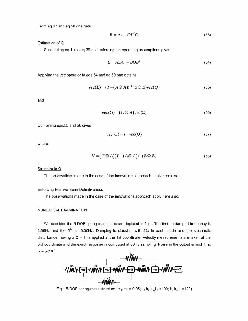
We co

2.66Hz an

disturbanc

3rd coordi

R = 5x10-4

47 and eq.50

n of Q

ituting eq.1 in

the vec opera

g eqs.55 and

in Q

bservations m

Positive Sem

bservations m

CAL EXAMINA

onsider the 5-

nd the 5th is

ce, having a Q

inate and the4.

Fig.1 5-DOF

one gets

nto eq.39 and

ator to eqs.54

(vec Σ

56 gives

V =

made in the ca

mi-Definitivene

made in the ca

ATION

-DOF spring-

s 16.30Hz. D

Q = 1, is app

exact respon

F spring-mass

ΛR =

enforcing the

Σ ΣA=

and eq.50 on

() (I AΣ = − ⊗

(( )vec G =

( )vec G

( )(C A I= ⊗

ase of the inn

ess

ase of the inn

-mass structu

Damping is c

plied at the 1s

nse is compu

s structure (m

10Λ CA G−−

e operating as

Σ T TA BQB+

ne obtains

) 1) (A B−⊗ ⊗

( ) (C A vec⊗

( )V vec Q= ⋅

) 1( )A A −− ⊗

novations app

novations app

ure depicted in

classical with

st coordinate.

ted at 50Hz s

m1-m5 = 0.05;

ssumptions g

) ( )B vec Q

( )Σ

( )B B⊗

proach apply h

proach apply h

n fig.1. The fi

2% in each

Velocity mea

sampling. Noi

k1,k3,k5,k7 =1

ives

here also.

here also.

irst un-dampe

h mode and

asurements a

ise in the outp

00; k2,k4,k6=1

(5

(5

(5

(5

(5

(5

ed frequency

the stochast

are taken at th

put is such th

120)

53)

54)

55)

56)

57)

58)

is

tic

he

hat

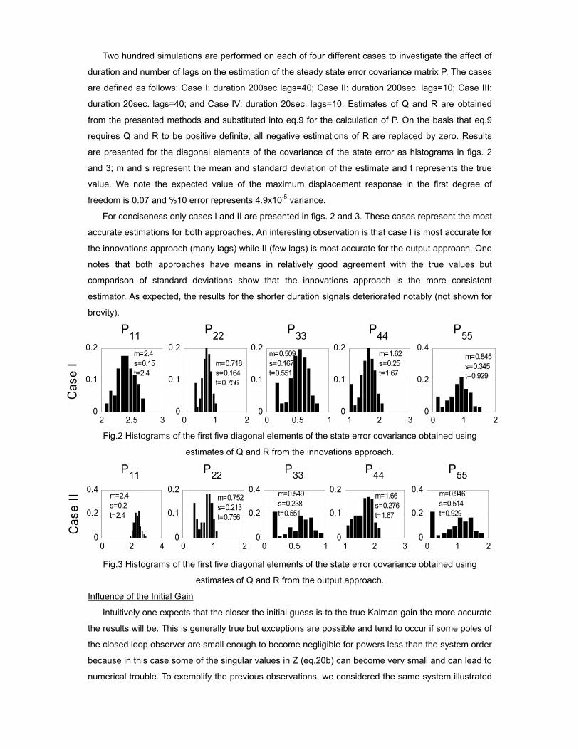
Two hundred simulations are performed on each of four different cases to investigate the affect of

duration and number of lags on the estimation of the steady state error covariance matrix P. The cases

are defined as follows: Case I: duration 200sec lags=40; Case II: duration 200sec. lags=10; Case III:

duration 20sec. lags=40; and Case IV: duration 20sec. lags=10. Estimates of Q and R are obtained

from the presented methods and substituted into eq.9 for the calculation of P. On the basis that eq.9

requires Q and R to be positive definite, all negative estimations of R are replaced by zero. Results

are presented for the diagonal elements of the covariance of the state error as histograms in figs. 2

and 3; m and s represent the mean and standard deviation of the estimate and t represents the true

value. We note the expected value of the maximum displacement response in the first degree of

freedom is 0.07 and %10 error represents 4.9x10-5 variance.

For conciseness only cases I and II are presented in figs. 2 and 3. These cases represent the most

accurate estimations for both approaches. An interesting observation is that case I is most accurate for

the innovations approach (many lags) while II (few lags) is most accurate for the output approach. One

notes that both approaches have means in relatively good agreement with the true values but

comparison of standard deviations show that the innovations approach is the more consistent

estimator. As expected, the results for the shorter duration signals deteriorated notably (not shown for

brevity).

Fig.2 Histograms of the first five diagonal elements of the state error covariance obtained using

estimates of Q and R from the innovations approach.

Fig.3 Histograms of the first five diagonal elements of the state error covariance obtained using

estimates of Q and R from the output approach.

Influence of the Initial Gain

Intuitively one expects that the closer the initial guess is to the true Kalman gain the more accurate

the results will be. This is generally true but exceptions are possible and tend to occur if some poles of

the closed loop observer are small enough to become negligible for powers less than the system order

because in this case some of the singular values in Z (eq.20b) can become very small and can lead to

numerical trouble. To exemplify the previous observations, we considered the same system illustrated

2 2.5 30

0.1

0.2m=2.4 s=0.15 t=2.4

Cas

e I

P11

0 1 20

0.1

0.2

P22

m=0.718 s=0.164 t=0.756

0 0.5 10

0.1

0.2

P33m=0.509 s=0.167 t=0.551

1 2 30

0.1

0.2

P44m=1.62 s=0.25 t=1.67

0 1 20

0.2

0.4

P55

m=0.845 s=0.345 t=0.929

P11 P22 P33 P44 P55

0 2 40

0.2

0.4m=2.4 s=0.2 t=2.4

Cas

e II

0 1 20

0.1

0.2m=0.752 s=0.213 t=0.756

0 0.5 10

0.2

0.4 m=0.549 s=0.238 t=0.551

1 2 30

0.1

0.2m=1.66 s=0.276 t=1.67

0 1 20

0.2

0.4 m=0.946 s=0.514 t=0.929

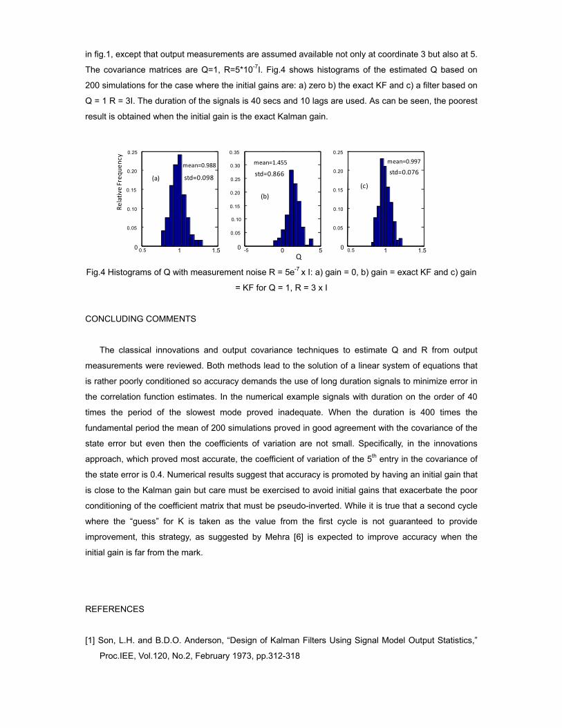
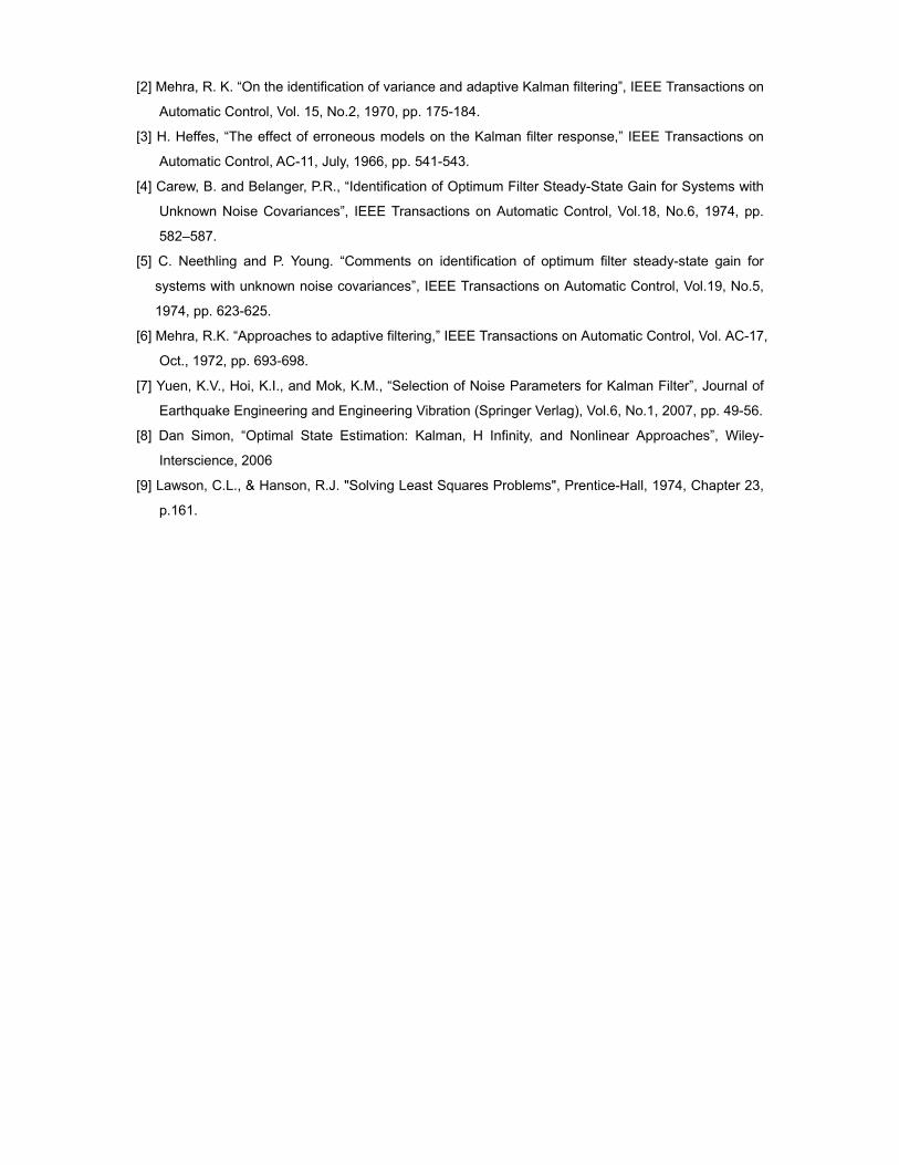
in fig.1, except that output measurements are assumed available not only at coordinate 3 but also at 5.

The covariance matrices are Q=1, R=5*10-7I. Fig.4 shows histograms of the estimated Q based on

200 simulations for the case where the initial gains are: a) zero b) the exact KF and c) a filter based on

Q = 1 R = 3I. The duration of the signals is 40 secs and 10 lags are used. As can be seen, the poorest

result is obtained when the initial gain is the exact Kalman gain.

Fig.4 Histograms of Q with measurement noise R = 5e-7 x I: a) gain = 0, b) gain = exact KF and c) gain

= KF for Q = 1, R = 3 x I

CONCLUDING COMMENTS

The classical innovations and output covariance techniques to estimate Q and R from output

measurements were reviewed. Both methods lead to the solution of a linear system of equations that

is rather poorly conditioned so accuracy demands the use of long duration signals to minimize error in

the correlation function estimates. In the numerical example signals with duration on the order of 40

times the period of the slowest mode proved inadequate. When the duration is 400 times the

fundamental period the mean of 200 simulations proved in good agreement with the covariance of the

state error but even then the coefficients of variation are not small. Specifically, in the innovations

approach, which proved most accurate, the coefficient of variation of the 5th entry in the covariance of

the state error is 0.4. Numerical results suggest that accuracy is promoted by having an initial gain that

is close to the Kalman gain but care must be exercised to avoid initial gains that exacerbate the poor

conditioning of the coefficient matrix that must be pseudo-inverted. While it is true that a second cycle

where the “guess” for K is taken as the value from the first cycle is not guaranteed to provide

improvement, this strategy, as suggested by Mehra [6] is expected to improve accuracy when the

initial gain is far from the mark.

REFERENCES

[1] Son, L.H. and B.D.O. Anderson, “Design of Kalman Filters Using Signal Model Output Statistics,”

Proc.IEE, Vol.120, No.2, February 1973, pp.312-318

(a) (b) (c)

Mean =0.988std =0.098

std =0.076

Mean =0.997Mean =1.455std =0.866

-5 0 50

0.05

0.10

0.15

0.20

0.25

0.30

0.35

0.5 1 1.50

0.05

0.10

0.15

0.20

0.25

0.5 1 1.50

0.05

0.10

0.15

0.20

0.25

std=0.098

mean=0.988 mean=1.455 mean=0.997

std=0.866 std=0.076(a)

(b)

(c)

Q

Relative Freq

uency

[2] Mehra, R. K. “On the identification of variance and adaptive Kalman filtering”, IEEE Transactions on

Automatic Control, Vol. 15, No.2, 1970, pp. 175-184.

[3] H. Heffes, “The effect of erroneous models on the Kalman filter response,” IEEE Transactions on

Automatic Control, AC-11, July, 1966, pp. 541-543.

[4] Carew, B. and Belanger, P.R., “Identification of Optimum Filter Steady-State Gain for Systems with

Unknown Noise Covariances”, IEEE Transactions on Automatic Control, Vol.18, No.6, 1974, pp.

582–587.

[5] C. Neethling and P. Young. “Comments on identification of optimum filter steady-state gain for

systems with unknown noise covariances”, IEEE Transactions on Automatic Control, Vol.19, No.5,

1974, pp. 623-625.

[6] Mehra, R.K. “Approaches to adaptive filtering,” IEEE Transactions on Automatic Control, Vol. AC-17,

Oct., 1972, pp. 693-698.

[7] Yuen, K.V., Hoi, K.I., and Mok, K.M., “Selection of Noise Parameters for Kalman Filter”, Journal of

Earthquake Engineering and Engineering Vibration (Springer Verlag), Vol.6, No.1, 2007, pp. 49-56.

[8] Dan Simon, “Optimal State Estimation: Kalman, H Infinity, and Nonlinear Approaches”, Wiley-

Interscience, 2006

[9] Lawson, C.L., & Hanson, R.J. "Solving Least Squares Problems", Prentice-Hall, 1974, Chapter 23,

p.161.