PROCEEDINGS OF THE ROYAL SOCIETY A

doi:10.1098/rspa.2010.0505

Structures buckling under tensile dead load

D. Zaccaria(1), D. Bigoni(2), G. Noselli(2) and D. Misseroni(2)

(1)Department of Civil and Environmental Engineering, University of Trieste

piazzale Europa 1, Trieste, Italy(2)Department of Mechanical and Structural Engineering, University of Trento

via Mesiano 77, Trento, Italy

Abstract

Some 250 years after the systematic experiments by Musschenbroek and their rationalizationby Euler, for the first time we show that it is possible to design structures (i.e. mechanicalsystems whose elements are governed by the equation of the elastica) exhibiting bifurcationand instability (‘buckling’) under tensile load of constant direction and point of application(‘dead’). We show both theoretically and experimentally that the behaviour is possible inelementary structures with a single degree of freedom and in more complex mechanical sys-tems, as related to the presence of a structural junction, called ‘slider’, allowing only relativetransversal displacement between the connected elements. In continuous systems where theslider connects two elastic thin rods, bifurcation occurs both in tension and compressionand is governed by the equation of the elastica, employed here for tensile loading, so thatthe deformed rods take the form of the capillary curve in a liquid, which is in fact gov-erned by the equation of the elastica under tension. Since axial load in structural elementsdeeply influences dynamics, our results may provide application to innovative actuators formechanical wave control, moreover, they open a new perspective in the understanding offailure within structural elements.

Keywords: Elastica, bifurcation, instability under tension

1 Introduction

Buckling of a straight elastic column subject to compressive end thrust occurs at a criticalload for which the straight configuration of the column becomes unstable and simultaneously

2Corresponding author: Davide Bigoni - fax: +39 0461 882599; tel.: +39 0461 882507; web-site: http://www.ing.unitn.it/∼bigoni/; e-mail: bigoni@ing.unitn.it.

1

ceases to be the unique solution of the elastic problem (so that instability and bifurcation areconcomitant phenomena). Buckling is known from ancient times: it has been experimentallyinvestigated in a systematic way by Pieter van Musschenbrok (1692-1761) and mathematicallysolved by Leonhard Euler (1707-1783), who derived the differential equation governing thebehaviour of a thin elastic rod suffering a large bending, the so-called ‘elastica’ (see Love,1927).

Through centuries, engineers have experimented and calculated complex structures, such asframes, plates and cylinders, manifesting instabilities and bifurcations of various forms (Tim-oshenko and Gere, 1961), so that certain instabilities have been found involving tensile loads.For instance, there are examples classified by Ziegler (1977) as ‘buckling by tension’ where atensile loading is applied to a system in which a compressed member is always present, so thatthey do not represent true bifurcations under tensile loads. Other examples given by Gajewskiand Palej (1974) are all related to the complex live (as opposed to ‘dead’) loading system, forinstance, loading through a vessel filled with a liquid, so that Zyczkowski (1991) points outthat ‘With Eulerian behaviour of loading (materially fixed point of application, direction fixedin space), the bar cannot lose stability at all [...].’ Note finally that necking of a circular barrepresents a bifurcation of a material element under tension, not of a structure.

It can be concluded that until now structures made up of line elements (each governed bythe equation of the elastica) exhibiting bifurcation and instability under tensile load of fixeddirection and point of application (in other words ‘dead’) have never been found, so that theword ‘buckling’ is commonly associated to compressive loads.

In the present article we show that:

• simple structures can be designed evidencing bifurcation (buckling) and instability undertensile dead loading;

• the deformed shapes of these structures can be calculated using the equation of the elas-tica, but under tension, so that the deflection of the rod is identical to the shape ofa capillary curve in a liquid, which is governed by the same equation, see Fig. 1 andSections 3.2 and 4;

• experiments show that elastic structures buckling under tension can be realized in practiceand that they closely follow theory predictions, Sections 2 and 4.

The above findings are complemented by a series of minor new results for which our sys-tem behaves differently from other systems made up of elastic rods, but with the usual endconditions. First, our system evidences load decrease with increase of axial displacement (theso-called ‘softening’), second, the bifurcated paths involving relative displacement at the sliderterminate at an unloaded limit configuration, for both tension and compression.

We will see that the above results follow from a novel use of a junction between mechanicalparts, namely, a slider or, in other words, a connection allowing only relative sliding (transversedisplacement) between the connected pieces and therefore constraining the relative rotation andaxial displacement to remain null.

Vibrations of structures are deeply influenced by axial load, so that the speed of flexuralwaves vanishes at bifurcation (Bigoni et al. 2008; Gei et al. 2009), a feature also evidenced

2

Fig. 1: Analogy between an elastic rod buckled under tensile force (left) and a water meniscus in a capillarychannel (right, superimposed to the solution of the elastica, marked in red): the deflection of the rod and thesurface of the liquid have the same shape, see Section 4.

by the dynamical analysis presented in Section 3.1, so that, since bifurcation is shown to occurin our structures both in tension and compression, these can be used as two-way actuators formechanical waves, where the axial force controls the speed of the waves traversing the structure.Therefore, the mechanical systems invented in the present article can immediately be generalizedand employed to design complex mechanical systems exhibiting bifurcations in tension andcompression, to be used, for instance, as systems with specially designed vibrational properties(a movie providing a simple illustration of the concepts exposed in this paper, together witha view of experimental results, is provided in the electronic supplementary material, see alsohttp://www.ing.unitn.it/dims/ssmg.php).

2 A simple single-degree-of-freedom structure which bucklesfor tensile dead loading

The best way to understand how a structure can bifurcate under tensile dead loading is toconsider the elementary single-degree-of-freedom structure shown in Fig. 2, where two rigidrods are connected through a ‘slider’ (a device which imposes the same rotation angle andaxial displacement to the two connected pieces, but null shear transmission, leaving only thepossibility of relative sliding).

Bifurcation load and equilibrium paths of this single-degree-of-freedom structure can becalculated by considering the bifurcation mode illustrated in Fig. 2 and defined by the rotationangle φ. The elongation of the system and the potential energy are respectively

∆ = 2l

(

1

cosφ− 1

)

and W (φ) =1

2kφ2 − 2Fl

(

1

cosφ− 1

)

, (1)

so that solutions of the equilibrium problem are

F =k φ cos2 φ

2l sinφ, (2)

for φ 6= 0, plus the trivial solution (φ = 0, ∀F ). Analysis of the second-order derivative of thestrain energy reveals that the trivial solution is stable up to the critical load

Fcr =k

2l, (3)

3

Fig. 2: Bifurcation of a single-degree-of-freedom elastic system under tensile dead loading (the rods of lengthl are rigid and jointed through a slider, a device allowing only for relative sliding between the two connectedpieces). A rotational elastic spring of stiffness k, attached at the hinge on the left, provides the elastic stiffness.Note that the bifurcation is ‘purely geometrical’ and is related to the presence of the constraint at the middleof the beam which transmits rotation, but not shear (left). The bifurcation diagram, showing bifurcation andsoftening in tension is reported on the right. The rotation angle φ0 = {1◦, 10◦} denotes an initial imperfection,in terms of an initial inclination of the two rods with respect to the horizontal direction.

while the nontrivial path, evidencing softening, is unstable. For an imperfect system, charac-terized by an initial inclination of the rods φ0, we obtain

W (φ, φ0) =1

2k (φ− φ0)

2 − 2Fl

(

1

cosφ− 1

cosφ0

)

and F =k (φ− φ0) cos

2 φ

2l sinφ, (4)

so that the force–rotation relation is obtained, which is reported as two dashed lines in Fig. 2for φ0 = 1◦ and φ0 = 10◦.

The simple structure presented in Fig. 2, showing possibility of a bifurcation under deadload in tension and displaying an overall softening behaviour, can be realized in practice, asshown by the wooden model reported in Fig. 3.

Fig. 3: A model of the single-degree-of-freedom elastic structure shown in Fig. 2 on the left (in which a metalstrip reproduces the rotational spring and the load is given through hanging a load) displaying bifurcation fortensile dead loading (left: undeformed configuration; right: buckled configuration).

4

3 Vibrations, buckling and the elastica for a structure subject

to tensile (and compressive) dead loading

In order to generalize the single-degree-of-freedom system model into an elastic structure, weconsider two inextensible elastic rods clamped at one end and jointed through a slider, identicalto that used to joitn the two rigid bars employed for the single-degree-of-freedom system (seethe inset of Fig. 4). The two bars have bending stiffness B, length l− (on the left) and l+ (onthe right) and are subject to a load F which may be tensile (F > 0) or compressive (F < 0).

3.1 The vibrations and critical loads

The differential equation governing the dynamics of an elastic rod subject to an axial force F(assumed positive if tensile) is

∂4v(z, t)

∂z4− F

B

∂2v(z, t)

∂z2+

ρ

B

∂2v(z, t)

∂t2= 0, (5)

where ρ is the unit-length mass density of the rod and v the transversal displacement, so thattime-harmonic motion is based on the separate-variable representation

v(z, t) = v(z) e−iωt, (6)

in which ω is the circular frequency, t is the time and i =√−1 is the imaginary unit.

A substitution of eqn (6) into eqn (5) yields the equation governing time-harmonic oscilla-tions

d4v(z)

dz4− α2 sign(F )

d2v(z)

dz2− βv(z) = 0, (7)

where the function ‘sign’ (defined as sign(α) = |α|/α ∀α ∈ Re and sign(0) = 0) has been usedand

α2 =|F |B

, β = ω2 ρ

B. (8)

The general solution of eqn (7) is

v(z) = C1 cosh(λ1z) + C2 sinh(λ1z) + C3 cos(λ2z) + C4 sin(λ2z), (9)

where

λ1 =

√

√

α4 + 4β + α2 sign(F )

2, λ2 =

√

√

α4 + 4β − α2 sign(F )

2. (10)

Eqn (9) holds both for the rod on the left (transversal displacement denoted with ‘−’) and onthe right (transversal displacement denoted with ‘+’) shown in the inset of Fig. 4, so that theboundary conditions at the clamps impose

v−(0) =dv−

dz

∣

∣

∣

∣

z=0

= 0, v+(l+) =dv+

dz

∣

∣

∣

∣

z=l+= 0, (11)

5

while at the slider we have the two conditions

d3v−

dz3

∣

∣

∣

∣

z=l−=

d3v+

dz3

∣

∣

∣

∣

z=0

= 0, (12)

expressing the vanishing of the shear force. The imposition of the six conditions (11)–(12)provides the constants C±

2,3,4 as functions of the constants C±

1 , so that the continuity of therotation at the slider

dv−

dz

∣

∣

∣

∣

z=l−=

dv+

dz

∣

∣

∣

∣

z=0

(13)

and the equilibrium of the slider

d2v−

dz2

∣

∣

∣

∣

z=l−− α2 sign(F ) v−(l−) =

d2v+

dz2

∣

∣

∣

∣

z=0

− α2 sign(F ) v+(0), (14)

yields finally a linear homogeneous system (with unknowns C−

1 and C+1 ), whose determinant

has to be set equal to zero, to obtain the frequency equation, function of α2, ω and sign(F ).The circular frequency ω (normalized through multiplication by

√

ρl4/B) versus the axialforce (normalized through multiplication by 4l2/(Bπ2)) is reported in Fig. 4, where the firstfour branches are shown for a system of two rods of equal length. In this figure the gray zones

Fig. 4: Dimensionless circular frequency ω for the structure shown in the inset (in the particular case of rodsof equal length, l) as a function of the dimensionless applied load F . Note that solutions in the gray regioncannot be achieved, since the rods cannot remain straight for axial forces external to the bifurcation range ofloads (shown as a white zone).

represent situations that cannot be achieved, in the sense that the axial force falls outside theinterval where the straight configuration of the system is feasible (in other words, for axialloads external to the interval of first bifurcations in tension and compression, the straightconfiguration cannot be maintained).

6

The branches shown in Fig. 4 intersect the horizontal axis in correspondence of the bifurca-tion loads of the system, namely, 4Fcrl

2/(π2B) = −16,−15.19,−4,−3.17,+0.58, so that thereis one critical load in tension (the corresponding branch is labeled ‘1st slider mode’ in Fig. 4),and infinitely many bifurcation loads in compression, the first three are reported in Fig. 4 (bi-furcations corresponding to the label ‘global mode’ do not involve relative displacement acrossthe slider).

Beside the possibility of bifurcation in tension, an interesting and novel effect related tothe presence of the slider is that a tensile (compressive) axial force yields a decrease (increase)of the frequency of the system, while an opposite effect is achieved when ‘global modes’ areactivated.

Quasi-static solutions of the system and related bifurcations can be obtained in the limitω → 0 of the frequency equation, which yields

tanh(

α l−)

cosh(

α l+)

+ sinh(

α l+) [

1− (l+ + l−)α tanh(

α l−)]

= 0, forF > 0,

tan(

α l−)

cos(

α l+)

+ sin(

α l+) [

1 + (l+ + l−)α tan(

α l−)]

= 0, forF < 0.

(15)

In the particular case of rods of equal length l, eqns (15) simplify to

sinh (α l) [1− α l tanh (α l)] = 0, forF > 0,

sin (α l) [1 + α l tan (α l)] = 0, forF < 0.

(16)

Eqns (16) show clearly that there is only one bifurcation load in tension (branch labeled‘1st slider mode’ in Fig. 4), but there are ∞2 bifurcation loads in compression (the first threebranches are reported in Fig. 4). In compression, the bifurcation condition sin (α l) = 0, pro-viding ∞1 solutions, yields the critical loads of a doubly clamped beam of length 2l and defineswhat we have labeled ‘global modes’ in Fig. 4.

Bifurcation loads, normalized through multiplication by (l+ + l−)2/(π2B), are reported inFig. 5 as functions of the ratio l+/l− between the lengths of the two rods. Note that the graphis plotted in a semi-logarithmic scale, which enforces symmetry about the vertical axis. In thegraph, the first two buckling loads in compression are reported: the first corresponds to a modeinvolving sliding, while the second does not involve any sliding (and when l+ = l− correspondsto the first mode of a doubly clamped rod of length 2l). Used as an optimization parameter,l+ = l− corresponds to the lower bifurcation load in tension (+0.58), near five times smaller(in absolute value) that the buckling load in compression (−3.17).

3.2 The elastica

The determination of the non-trivial configurations at large deflections of the mechanical sys-tem requires a careful use of Euler’s elastica. It is instrumental to employ the reference systemsshown in Fig. 6 and impose one kinematic compatibility condition and three equilibrium con-ditions. These are as follows.

7

1st

slider mode

1st

slider mode

1st

global mode

0.58

-3.17

-1

-4

0.01 0.1 1 10 100

-10

-5

0

5

0.01 0.1 1 10 100

Fcr(

-+

+(

B)

p2

ll

)/

2

- / +l l

Fig. 5: Dimensionless critical loads Fcr as a function of the ratio between the lengths of the rods, l+/ l−. Thedimensionless axial forces for bifurcation in tension and those corresponding to the first two modes in compressionare reported.

Fig. 6: Sketch of the problem of the elastica under tensile axial load F . Note the reference systems employed inthe analysis and note that the moments on the slider have been reported positive and the curvature results tobe negative.

• The kinematic compatibility condition can be directly obtained from Fig. 6 noting that thejump in displacement across the slider (measured orthogonally to the line of the elastica),∆s, can be related to the angle of rotation of the slider Φs, a condition that assuming thelocal reference systems shown in Fig. 6 becomes

[

x−1 (l−) + x+1 (l

+)]

tanΦs + x−2 (l−) + x+2 (l

+) + ∆s = 0, (17)

8

where x1(s) and x2(s) are the coordinates of the elastica and the index − (+) denotesthat the quantities are referred to the rod on the left (on the right). Note that Φs isassumed positive when anticlockwise and ∆s is not restricted in sign (negative in the caseof Fig. 6).

• Since the slider can only transmit a moment and a force R orthogonal to it, equilibriumrequires that (see the inset in Fig. 6)

R =F

cos Φs

, (18)

where F is the axial force providing the load to the rod, assumed positive (negative) whentensile (compressive), so that since Φs ∈ [−π/2, π/2], R is positive (negative) for tensile(compressive) load. Note that with the above definitions we have

θ+(0) = θ−(0) = 0, θ+(l+) = θ−(l−) = −Φs. (19)

• Equilibrium of the slider requires that

κ−s + κ+s =R

B∆s, (20)

where B is the bending stiffness of the rod and κ±s is the curvature on the left (−) or onthe right (+) of the slider. Note that B is always positive, but R, κ±s and ∆s can takeany sign.

• For both rods (left and right) rotational equilibrium of the element of rod singled out atcurvilinear coordinate s requires

d 2θ

ds 2− R

Bsin θ = 0, (21)

where θ is the rotation of the normal at each point of the elastica, assumed positive whenanticlockwise, with added the superscript − (+) to denote the rod on the left (on theright).

Eqn (21) is usually (see for instance Love, 1927, his eqn (8) at Sect. 262) written with asign ‘+’ replacing the sign ‘−’ and R is assumed positive when compressive; the same equationdescribes the motion of a simple pendulum (see for instance Temme, 1996). The ‘+’ signoriginates from the fact that the elastica has been analyzed until now only for deformationsoriginating from compressive loads. However, an equation with the ‘−’ sign and with R/Breplaced by the ratio between unit weight density and surface tension of a fluid –thus equal toeqn (21)– determines the shape of the capillary curve of a liquid (Lamb, 1928), which thereforeresults to be identical to the deflection of a rod under tensile load.

In the following we derive equations holding along both rods ‘+’ and ‘−’, so that theseindices will be dropped for simplicity. Multiplication of eqn (21) by d θ/ds and integration from0 to s yields

(

d θ

d s

)2

= −2 α2 sign(R) cos θ + 2 α2

(

2

k2− 1

)

, (22)

9

where, using the Heaviside step function H, we have

α2 =|R|B

and k2 =

(

κ2s4 α2

+H(R)

)−1

. (23)

Eqn (22) can be re-written as(

d θ

d s

)2

=4 α2

k2

[

1− k2 sin2(

θ

2+

π

2H(R)

)]

, (24)

so that the change of variable u = sα/k yields

d θ

d u= ±2

√

1− k2 sin2(

θ

2+

π

2H(R)

)

. (25)

The analysis will be restricted for simplicity to the case ‘+’ in the following. At u = 0 it isθ = 0, so that eqn (25) gives the solution

θ = 2am [u+KH(R), k]− πH(R) andd θ

d s=

2

kα dn [u+KH(R), k] , (26)

where am and dn are respectively the Jacobi elliptic functions amplitude and delta-amplitudeand K is the complete elliptic integral of the first kind (Byrd and Friedman, 1971). Since inthe local reference system we have dx1/ds = cos θ and dx2/ds = sin θ, an integration gives thecoordinates x1 and x2 of the elastica expressed in terms of u,

x1 =1

k α

[(

2− k2)

u− 2E [am [u, k] , k] + 2k2sn [u, k] cn [u, k]]

x2 =2

k α

√

1− k2(

1− dn [u, k]

dn [u, k]

)

forR > 0, (27)

for tensile axial loads, while for compressive axial loads

x1 =1

k α

[(

k2 − 2)

u+ 2E [am [u, k] , k]]

x2 =2

k α(1− dn [u, k])

forR < 0, (28)

in which the constants of integration are chosen so that x1 and x2 vanish at s = 0. In eqns (27)–(28) sn and cn are respectively the Jacobi elliptic functions sine-amplitude and cosine-amplitudeand E is the incomplete elliptic integral of the second kind (Byrd and Friedman, 1971).

Eqns (28) differ from eqns (16) reported by Love (1927, his Section 263) only in a translationof the coordinate x2, while eqns (27), holding for tensile axial force, are new.

Finally, with reference to Fig. 6, we note that the horizontal displacement ∆c of the rightclamp can be written in the form

∆c =x−1 (l

−) + x+1 (l+)

cos Φs

−(

l+ + l−)

. (29)

To find the axial load F as a function of the slider rotation Φs, or as a function of the enddisplacement ∆c, we have now to proceed as follows:

10

• values for κ−s and κ+s are fixed (as a function of the selected mode, for instance, κ−s = κ+s ,to analyze the bifurcation mode in tension);

• k can be expressed using eqn (23) as a function of α;

• the equations for the coordinates of the elastica, eqn (27) for tensile load, or eqn (28) forcompressive load, and eqn (26)1, evaluated at l− and l+, become functions of only α;

• eqns (19) and (20) provide Φs and ∆s, so that eqn (17) becomes a nonlinear equation inthe variable α, which can be numerically solved (we have used the function FindRoot ofMathematica R© 6.0);

• when α is known, R and F can be obtained from eqns (23) and (18);

• finally, Φs and ∆c are calculated using eqns (19) and (29).

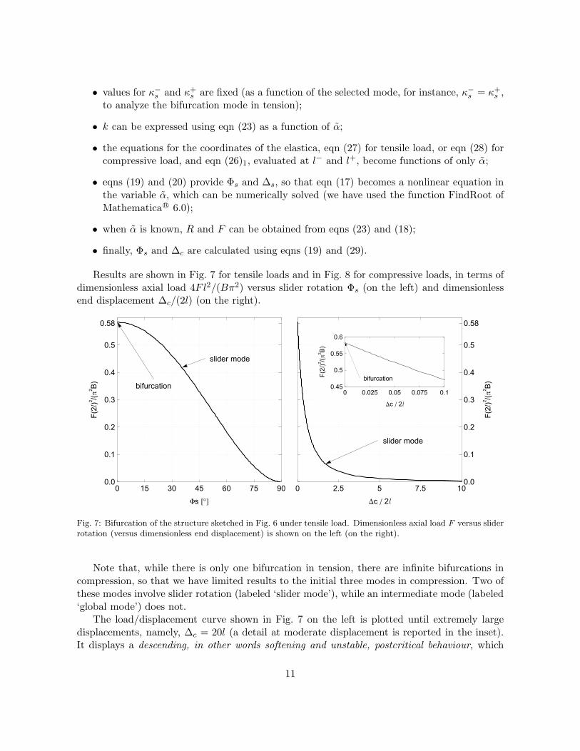
Results are shown in Fig. 7 for tensile loads and in Fig. 8 for compressive loads, in terms ofdimensionless axial load 4Fl2/(Bπ2) versus slider rotation Φs (on the left) and dimensionlessend displacement ∆c/(2l) (on the right).

slider mode

0 2.5 5 7.5 100.0

0.1

0.2

0.3

0.4

0.5

0.58

Dc � 2l

bifurcation

0 0.025 0.05 0.075 0.10.45

0.5

0.55

0.6

Dc � 2l

slider mode

bifurcation

0 15 30 45 60 75 900.0

0.1

0.2

0.3

0.4

0.5

0.58

Fs @°D

F2(l

22

)/(

B)

p

F2(l

22

)/(

B)

p

F2(l

22

)/(

B)

p

Fig. 7: Bifurcation of the structure sketched in Fig. 6 under tensile load. Dimensionless axial load F versus sliderrotation (versus dimensionless end displacement) is shown on the left (on the right).

Note that, while there is only one bifurcation in tension, there are infinite bifurcations incompression, so that we have limited results to the initial three modes in compression. Two ofthese modes involve slider rotation (labeled ‘slider mode’), while an intermediate mode (labeled‘global mode’) does not.

The load/displacement curve shown in Fig. 7 on the left is plotted until extremely largedisplacements, namely, ∆c = 20l (a detail at moderate displacement is reported in the inset).It displays a descending, in other words softening and unstable, postcritical behaviour, which

11

1st slider mode

2nd slider mode

1st global mode

bifurcations

0-0.25-0.5-0.75-1

0.0

-3.17-4-5

-10

-15

-20

Dc � 2l

1st slider mode

2nd slider mode

bifurcations

0 15 30 45 60 75 90

0.0

-3.17

-5

-10

-15

-20

Fs @°D

F2(l

22

)/(

B)

p

F2(l

22

)/(

B)

p

Fig. 8: Bifurcation of the structure sketched in Fig. 6 under compressive load. Dimensionless axial load F versusslider rotation (versus dimensionless end displacement) is shown on the left (on the right).

contrasts with the usual postcritical of the elastica under various end conditions, in which theload rises with displacement. In compression, the post-critical behaviour evidences anothernovel behaviour, so that the first and the second slider modes present an initial part wherethe load/displacement rises, followed by a softening behaviour. Finally, it is important to notethat the curves load versus Φs in Figs. 7 and 8, both for tension and compression intersecteach other at null loading at the extreme rotation Φs = 90◦, which means that two unloadedconfigurations (in addition to the initial configuration) exist. These peculiarities, never observedbefore in simple elastic structures, are all related to the presence of the slider.

Deformed elastic lines are reported in Fig. 9, both for tension and compression, the lattercorresponding to the first three slider modes (the global mode is not reported since it corre-sponds to the first mode of a doubly-clamped rod).

4 Experimental

The structure sketched in Fig. 6 has been realized with two carbon steel AISI 1095 strips (250mm × 25 mm × 1 mm; Young modulus 200 GPa) and the slider with two linear bearings(type Easy Rail SN22-80-500-610, purchased from RollonR©), commonly used in machine designapplications, see the inset of Fig. 10. The slider is certified by the producer to have a lowfriction coefficient, equal to 0.01. Tensile force on the structure has been provided by imposingdisplacement with a load frame ELE Tritest 50 (ELE International Ltd), the load measuredwith a load cell Gefran OC-K2D-C3 (Gefran Spa), and the displacement with a potentiometrictransducer Gefran PY-2-F-100 (Gefran Spa). Data have been acquired with system NI Com-pactDAQ, interfaced with Labview 8.5.1 (National Instruments). Photos have been taken witha Nikon D200 digital camera, equipped with a AF-S micro Nikkor lens (105 mm 1:2.8G ED)

12

Slider

tensile mode-0.2

-0.1

0.0

0.1

0.2

Slider

1st mode

Slider2nd mode

-0.6 -0.4 -0.2 0.0 0.2 0.4 0.6

-0.2

-0.1

0.0

0.1

0.2

@2lD

Slider3rd mode

-0.6 -0.4 -0.2 0.0 0.2 0.4 0.6

@2lD

@2lD

@2lD

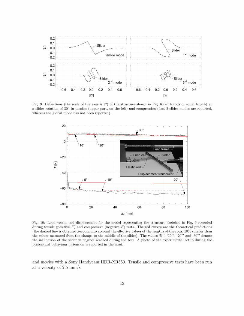
Fig. 9: Deflections (the scale of the axes is 2l) of the structure shown in Fig. 6 (with rods of equal length) ata slider rotation of 30◦ in tension (upper part, on the left) and compression (first 3 slider modes are reported,whereas the global mode has not been reported).

Fig. 10: Load versus end displacement for the model representing the structure sketched in Fig. 6 recordedduring tensile (positive F ) and compressive (negative F ) tests. The red curves are the theoretical predictions(the dashed line is obtained keeping into account the effective values of the lengths of the rods, 10% smaller thanthe values measured from the clamps to the middle of the slider). The values ‘5◦’, ‘10◦’, ‘20◦’ and ‘30◦’ denotethe inclination of the slider in degrees reached during the test. A photo of the experimental setup during thepostcritical behaviour in tension is reported in the inset.

and movies with a Sony Handycam HDR-XR550. Tensile and compressive tests have been runat a velocity of 2.5 mm/s.

13

Photos taken at different slider rotations (and thus load levels) are shown in Fig. 11 fortension (Φs = 0◦, 10◦, 20◦, 30◦) and in Fig. 12 for compression (Φs = 0◦, 5◦, 10◦, 20◦). Acomparison between theoretical predictions and experiments is reported in the lower parts ofthe figures where photos are superimposed to the line of the elastica, shown in red and plottedusing eqn (27) for tensile load and eqn (28) for compression.

Fig. 11: Photos of the model representing the structure sketched in Fig. 6 and loaded in tension at differentvalues of slider rotation Φs = 0◦, 10◦, (upper part) 20◦, 30◦ (center). The elastica calculated with eqn (27) issuperimposed on the photos at 20◦, 30◦ in the lower part. The side of the grid marked on the paper is 10 mm.

Fig. 12: Photos of the model representing the structure sketched in Fig. 6 and loaded in compression at differentvalues of slider rotation Φs = 0◦, 5◦, (upper part) 10◦, 20◦ (center). The elastica calculated with eqn (27) issuperimposed on the photos at 10◦, 20◦ in the lower part. The side of the grid marked on the paper is 10 mm.

These experiments show clearly the existence of the bifurcation in tension and provide anexcellent comparison with theoretical results obtained through integration of the elastica bothin tension and in compression. A further quantitative comparison between theoretical resultsand experiments is provided in Fig. 10, where the axial load in the structure (positive for tensionand negative for compression) is plotted versus the end displacement ∆c. The experimentalresult is compared to theoretical results (marked red) expressed by eqn (29), used in the waydetailed at the end of Section 3.2.

The theoretical result marked in red with continuous curve has been calculated assumingan initial length of the rods (25 cm) measured from the end of the clamps to the middle of theslider. However, the slider and the junctions to the metal strips are 58 mm thick, so that the

14

system is stiffer in reality. Therefore, we have plotted dashed the theoretical results obtainedemploying an ‘effective’ initial length of the rods reduced of 10% (so that the effective lengthof the system has been taken equal to 45 cm). The experimental curve evidences oscillationsof ±1 N for tensile loads and ±5 N for compressive loads. These oscillations are due to frictionwithin the slider, so that it is obvious that the oscillations are higher in compression than intension, since in the former case the load is higher. Except for these oscillations, the friction(which is very low) has been found not to influence the tests.

The fact that experimentally the bifurcations initiate before the theoretical values are at-tained represents the well-known effect of imperfections, so that we may conclude that theagreement between theory and experiments is excellent.

To provide experimental evidence to the fact that the elastica in tension corresponds to theshape of the free surface of a liquid in a capillary channel, we note that a meniscus in a capillarychannel satisfies (by symmetry) a null-rotation condition at the centre of the channel, so that itcorresponds to a clamped edge of a rod. If the tangent to the meniscus at the contact with thechannel wall is taken to correspond to the rotation of the non-clamped edge of the rod and thewidth of the channel is calculated employing the elastica, the elastic deflection of the rod scaleswith the free surface of the liquid. Therefore, we have performed an experiment in which wehave taken a photo (with a Nikon SMZ800 stereo-zoom microscope equipped with Nikon PlanApo 0.5x objective and a Nikon DD-FI1 high definition color camera head) of a water meniscusin a polycarbonate channel. We have proceeded as follows. First, we have observed that thecontact angle between a water surface in air and polycarbonate (at a temperature of 20◦C)is 70◦. Second, we have taken a photo of the meniscus formed in a polycarbonate ‘V-shaped’channel with walls inclined at 10◦ with the vertical, so that the angle between the horizontaldirection and the free surface results to be 30◦ and the distance between the walls results 6mm. This photo has been compared with a photo taken (with a Nikon D200 digital camera,and shown in Fig. 11 on the right) during buckling in tension when the elastic rods form thesame angle of 30◦. The result is shown in Fig. 1, together with the theoretical solution shownred.

Conclusions

We have theoretically proven and fully experimentally confirmed that elastic structures can bedesigned and practically realized in which bifurcation can occur with tensile dead loading. Inthese structures no parts subject to compression are present. The finding is directly linked tothe presence of a junction allowing only for relative sliding between two parts of the mechanicalsystem. Our findings open completely new and unexpected perspectives, related for instance tothe control of the propagation of mechanical waves and to the understanding of certain failuremodes in material elements.

Acknowledgments

The authors gratefully acknowledge financial support from PRIN grant No. 2007YZ3B24.

15

References

[1] Bigoni, D., Gei, M. and Movchan, A.B. (2008) Dynamics of a prestressed stiff layer onan elastic half space: filtering and band gap characteristics of periodic structural modelsderived from long-wave asymptotics. J. Mech. Phys. Solids, 56, 2494-2520.

[2] Byrd, P.F and Friedman, M.D. (1971) Handbook of elliptic integrals for engineers andscientists. Springer-Verlag.

[3] Gajewski, A. and Palej, R. (1974) Stability and shape optimization of an elasticallyclamped bar under tension (in Polish). Rozprawy Inzynierskie - Engineering Transactions,22, 265-279.

[4] Gei, M., Movchan, A.B. and Bigoni, D. (2009) Band-gap shift and defect-induced annihi-lation in prestressed elastic structures. J. Appl. Phys., 105, 063507.

[5] Lamb, H. (1928) Statics. Cambridge University Press.

[6] Love, A.E.H. (1927) A treatise on the mathematical theory of elasicity. Cambridge Univer-sity Press.

[7] Temme, N.M. (1996) Special functions. John Wiley and Sons, New York.

[8] Timoshenko, S.P. and Gere, J.M. (1961) Theory of elastic stability. McGraw-Hill, NewYork.

[9] Ziegler, H. (1977) Principles of structural stability. Birkauser Verlag.

[10] Zyczkowski, M. (1991) Strength of structural elements. Elsevier.

16