PROCEEDINGS OF THEXIII GLOBAL OPTIMIZATION WORKSHOP

GOW’16

4-8 September 2016

Edited by

Ana Maria A. C. RochaUniversity of Minho/Algoritmi Research Centre

M. Fernanda P. CostaUniversity of Minho/Centre of Mathematics

Edite M. G. P. FernandesAlgoritmi Research Centre

ISBN: 978-989-20-6764-3University of Minho, Braga, Portugal

Preface

Past Global Optimization Workshops have been held in Sopron (1985 and 1990), Szeged (WGO,1995), Florence (GO’99, 1999), Hanmer Springs (Let’s GO, 2001), Santorini (Frontiers in GO,2003), San José (Go’05, 2005), Mykonos (AGO’07, 2007), Skukuza (SAGO’08, 2008), Toulouse(TOGO’10, 2010), Natal (NAGO’12, 2012) and Málaga (MAGO’14, 2014) with the aim of stim-ulating discussion between senior and junior researchers on the topic of Global Optimization.

In 2016, the XIII Global Optimization Workshop (GOW’16) takes place in Braga and is orga-nized by three researchers from the University of Minho. Two of them belong to the SystemsEngineering and Operational Research Group from the Algoritmi Research Centre and theother to the Statistics, Applied Probability and Operational Research Group from the Centreof Mathematics. The event received more than 50 submissions from 15 countries from Europe,South America and North America.

We want to express our gratitude to the invited speaker Panos Pardalos for accepting theinvitation and sharing his expertise, helping us to meet the workshop objectives. GOW’16would not have been possible without the valuable contribution from the authors and theInternational Scientific Committee members. We thank you all.

This proceedings book intends to present an overview of the topics that will be addressed inthe workshop with the goal of contributing to interesting and fruitful discussions between theauthors and participants. After the event, high quality papers can be submitted to a specialissue of the Journal of Global Optimization dedicated to the workshop.

Ana Maria A. C. RochaM. Fernanda P. CostaEdite M. G. P. Fernandes

GOW’16 Organizers

iv Preface

Preface v

Scientific Committee:Panos M. Pardalos, University of Florida (USA)Christodoulos A. Floudas, Texas A&M University (USA)Boris Mordukhovich, Wayne State University (USA)Nikolaos V. Sahinidis, Carnegie Mellon University (USA)David Gao, Federation University Australia (Australia)Ruey-Lin Sheu, National Cheng-Kung University (Taiwan)Sergiy Butenko, Texas A&M University (USA)Ana Maria A. C. Rocha, University of Minho (Portugal)Chrysanthos E. Gounaris, Carnegie Mellon University (USA)Ding-zhu Du, University of Texas (USA)Nicolas Hadjisavvas, King Fahd University of Petroleum and Minerals (Saudi Arabia)Fulop János, Hungarian Academy of Sciences (Hungary)Inmaculada G. Fernandez, University of Malaga (Spain)Alexander Mitsos, RWTH Aachen University (Germany)Dumitru Motreanu, University of Perpignan (France)Steffen Rebennack, Colorado School of Mines (USA)Mauricio G. C. Resende, AT&T Labs Research (USA)Leo Liberti, IBM T.J. Watson Research Center (USA)Yaroslav D. Sergeyev, University of Calabria (Italy)Fabio Schoen, University of Florence (Italy)Kaisa Miettinen, University of JyvÃd’skylÃd’ (Finland)Immanuel Bomze, University of Vienna (Austria)M. Fernanda P. Costa, University of Minho (Portugal)Angelo Lucia, University of Rhode Island (USA)Stratos Pistikopoulos, Texas A&M University (USA)Antanas Zilinskas, Vilnius University (Lithuania)Leonidas Pitsoulis, Aristotle University of Thessaloniki (Greece)Julius Zilinskas, Vilnius University (Lithuania)Edite M.G.P. Fernandes, University of Minho (Portugal)Igor Konnov, Kazan Federal University (Russia)Hoang Tuy, Institute of Mathematics (Vietnam)Paul I. Barton, Massachusetts Institute of Technology (USA)Michel Théra, University of Limoges (France)Erhun Kundakcioglu, Ozyegin University (Turkey)Simge Kucukyavuz, Ohio State University (USA)Tapio Westerlund, Åbo Akademi University (Finland)W. Art Chaovalitwongse, University of Washington (USA)Juan Enrique Martínez-Legaz, Universitat Autónoma de Barcelona (Spain)Marco Locatelli, University of Parma (Italy)Gianni Di Pillo, Sapienza University of Rome (Italy)Aris Daniilidis, University of Chile (Chile)Sofia Giuffrè, Mediterranea University of Reggio Calabria (Italy)Antonino Maugeri, University of Catania (Italy)Joaquim Júdice, University of Coimbra (Portugal)Anthony Man-Cho So, Chinese University of Hong Kong (China)C. Audet, Polytechnique Montreal (Canada)Janos D. Pintér, Saint Mary’s University (Canada)Francesco Zirilli, Sapienza University of Rome (Italy)Adil Bagirov, University of Ballarat (Australia)Eligius M. T. Hendrix, University of Malaga (Spain)J. Valério de Carvalho, University of Minho (Portugal)

vi Preface

Boris Goldengorin, Ohio University (USA)Mirjam Dur, University of Trier (Germany)Montaz Ali, University of the Witwatersrand (South Africa)Dmitri E. Kvasov, University of Calabria (Italy)

Organizing Committee:

Ana Maria A. C. RochaM. Fernanda P. CostaEdite M. G. P. Fernandes

Sponsors:

School of EngineeringDepartment of Production and SystemsAlgoritmi Research CentreSchool of SciencesDepartment of Mathematics and ApplicationsCentre of MathematicsUniversity of MinhoCâmara Municipal de BragaLibware

Contents

Preface iii

Invited Talk

On the Passage from Local to Global in Optimization: New Challenges in Theory and Practice 3Panos M. Pardalos

Extended Abstracts

The Cluster Problem in Constrained Global Optimization 9Rohit Kannan and Paul I. Barton

Distance Geometry: Too Much is Never Enough 13Gustavo Dias and Leo Liberti

Testing Pseudoconvexity via Interval Computation 17Milan Hladík

A Preference-Based Multi-Objective Evolutionary Algorithm for Approximating a Region ofInterest 21Ernestas Filatovas, Olga Kurasova, Juana López Redondo and José Fernández

Energy-Aware Computation of Evolutionary Multi-Objective Optimization 25G. Ortega, J.J. Moreno, E. Filatovas, J.A. Martínez and E.M. Garzón

Locating a Facility with the Partially Probabilistic Choice Rule 29José Fernández, Boglárka G.-Tóth, Juana López Redondo and Pilar Martínez Ortigosa

On Regular Refinement of Unit Simplex by just Visiting Grid Points 33L.G. Casado, J.M.G. Salmerón, B.G.-Tóth, E.M.T. Hendrix and I. García

Metabolic Pathway Analysis Using Nash Equilibrium 37Angelo Lucia and Peter A. DiMaggio

On Metaheuristics for Longest Edge Bisection of the Unit Simplex to Minimise the Search TreeSize 41J.M.G. Salmerón, J.L. Redondo, E.M.T. Hendrix and L.G. Casado

On Regular Simplex Division in Solving Blending Problems 45J.M.G. Salmerón, L.G. Casado, E.M.T. Hendrix and J.F.R Herrera

Strengthening Convex Relaxations of Mixed Integer Non Linear Programming Problems withSeparable Non Convexities 49Claudia D’Ambrosio, Antonio Frangioni and Claudio Gentile

Statistical Models for Global Optimization: How to Chose an Appropriate One ? 53

viii Contents

Antanas Žilinskas and Gražina Gimbutiene

A Branch-and-Bound Algorithm for Bi-Objective Problems 57Julia Niebling and Gabriele Eichfelder

On Achieving a Desired Flux Distribution on the Receiver of a Solar Power Tower Plant 61N.C. Cruz, J.L. Redondo, J.D. Álvarez, M. Berenguel and P.M. Ortigosa

The Alternating Direction Column Generation Method (Global Optimization without Branch-and-Bound) 65Ivo Nowak and Norman Breitfeld

Optimization of Enzymes Inactivation in High Pressure Processes 69Miriam R. Ferrández, Juana L. Redondo, Benjamin Ivorra, Ángel M. Ramos and Pilar M. Ortigosa

An Integrality Gap Minimization Heuristic for Binary Mixed Integer Nonlinear Programming 73Wendel Melo, Marcia Fampa and Fernanda Raupp

On B&B Algorithms in Greenhouse Climate Control 77Marleen Hermelink, Eligius M. T. Hendrix and Rene Haijema

On sBB Branching for Trilinear Monomials 81Emily Speakman and Jon Lee

Operational Zones for Global Optimization Algorithms 85Yaroslav D. Sergeyev, Dmitri E. Kvasov and Marat S. Mukhametzhanov

On Difference of Convex Optimization to Visualize Statistical Data and Dissimilarities 89Emilio Carrizosa, Vanesa Guerrero and Dolores Romero Morales

Extensions on Ellipsoid Bounds for Quadratic Programs 93Marcia Fampa and Francisco Pinillos Nieto

Solving MINLP Problems by a Penalty Framework 97Ana Maria A.C. Rocha, M. Fernanda P. Costa and Edite M.G.P. Fernandes

Improvements to the Supporting Hyperplane Optimization Toolkit Solver for Convex MINLP 101Andreas Lundell, Jan Kronqvist and Tapio Westerlund

Multiobjective Based Scoring Function for Ligand Based Virtual Screening 105Savíns P. Martín, Juana L. Redondo, Helena den-Haan A., Horacio Pérez-Sánchez and Pilar M. Ortigosa

lsmear: A Variable Selection Strategy for Interval Branch and Bound Solvers 109Ignacio Araya and Bertrand Neveu

Merging Flows in Terminal Manoeuvring Areas via Mixed Integer Linear Programming 113Mohammed Sbihi, Marcel Mongeau, Ma Ji and Daniel Delahaye

Lifted Polyhedral Approximations in Convex Mixed Integer Nonlinear Programming 117Jan Kronqvist, Andreas Lundell and Tapio Westerlund

Preference-based Multi-Objective Single Agent Stochastic Search 121Algirdas Lancinskas and Julius Žilinskas

Contents ix

A Quadratic Approach to the Maximum Edge Weight Clique Problem 125Seyedmohammadhossein Hosseinian, Dalila B.M.M. Fontes and Sergiy Butenko

Runtime Landscape Analysis for Global Optimization using Memetic Approaches 129Federico Cabassi and Marco Locatelli

An Interval Branch and Bound Algorithm for Parameter Estimation 133Bertrand Neveu, Martin de la Gorce and Gilles Trombettoni

Solving the 1-median Problem on a Network with Demand Surplus 137Kristóf Kovács, Rafael Blanquero, Emilio Carrizosa and Boglárka G.-Tóth

MILP Model for Batch Scheduling on Parallel Machines 141Renan S. Trindade, Olinto Araújo, Marcia Fampa and Felipe Müller

A Clustering-Based Algorithm for Aircraft Conflict Avoidance 145Sonia Cafieri and Emilio Carrizosa

On Solving Aircraft Conflict Avoidance Using Deterministic Global Optimization (sBB) Codes 149Sonia Cafieri, Frédéric Messine and Ahmed Touhami

Improving Performance of DIRECT-type Algorithms 153Remigijus Paulavicius and Julius Žilinskas

On the Beam Angle Optimization Problem in IMRT: Combinatorial vs Continuous Optimiza-tion 155H. Rocha, J. M. Dias, T. Ventura, B. C. Ferreira and M. C. Lopes

Parallel Implementation of GLOBAL with Applications to Nanophotonical Detector Develop-ment 159Tibor Csendes, Balázs Bánhelyi, Mária Csete, Dániel Zombori, Gábor Szabó and András Szenes

On Regular Simplex Refinement in Copositivity Detection 163J.M.G. Salmerón, P. Amaral, L.G. Casado, E.M.T. Hendrix and J. Žilinskas

A Numerical Analysis of Flocking Based Distributed Stochastic Optimization Algorithms OnNon-Convex Problems 167Charles Hernandez and Alfredo Garcia

A New Global Optimization Algorithm for Diameter Minimization Clustering 171Daniel Aloise and Claudio Contardo

Global Optimization of Continuous Minimax Problem 175Dominique Monnet, Jordan Ninin and Benoit Clement

Core-Based Upper Bounds for the Maximum Clique Problem 179Chitra Balasubramaniam, Balabhaskar Balasundaram and Sergiy Butenko

Session: Complex Solution Patterns for Standard Quadratic Optimization

Finding and Analyzing Hard Instances of the Standard Quadratic Optimization Problem 185Immanuel Bomze, Werner Schachinger and Reinhard Ullrich

Constructing Standard Quadratic Optimization Problems with Many Local Solutions 189Werner Schachinger, Immanuel Bomze and Reinhard Ullrich

x Contents

Complexity of a Standard Quadratic Problem: a Theory-Guided Experimental Study 193Reinhard Ullrich, Immanuel Bomze and Werner Schachinger

Topic Index 197

Author Index 199

INVITED TALK

Proceedings of GOW’16, pp. 3 – 5.

On the Passage from Local to Global in Optimization:New Challenges in Theory and Practice

Panos M. Pardalos 1

1Center for Applied Optimization, ISE Department,303 Weil Hall, University of Florida, Gainesville, FL 32611,http://www.ise.ufl.edu/pardalos, pardalos@ise.ufl.edu

Abstract Large scale problems in the design of networks and energy systems, the biomedical field, finance,and engineering are modeled as optimization problems. Humans and nature are constantly opti-mizing to minimize costs or maximize profits, to maximize the flow in a network, or to minimize theprobability of a blackout in the smart grid.

Due to new algorithmic developments and the computational power of computers, optimizationalgorithms have been used to solve problems in a wide spectrum of applications in science and engi-neering. In this talk I am going to address new challenges in the theory and practice of optimization.First, we have to reflect back a few decades to see what has been achieved and then address the newresearch challenges and directions.

Keywords: Global optimization,Local optimization, Complexity issues, Challenging problems

1. Global Optimization Problem

f∗ = f(x∗) = global minx∈Df(x) (or maxx∈Df(x)) (1)

For these global optimization problem we are going to address the following tasks:

Compute a globally optimal solution.

Compute "good" locally optimal solutions (or feasible points that satisfy the optimalityconditions).

Compute "better" solutions than "known" solutions.

Check feasibility of the constraints.

For the first case we will discuss complexity issues and the need of certificates of optimality.In addition, we are going to discuss classes of problems where only globally optimal solutionsare needed (or make sense). Furthermore, we are going to discuss recent progress and openquestions regarding exact algorithms.

The next two cases are of great practical significance. We can use approximation algorithmsor heuristics. We are going to discuss issues regarding the evaluation of the performance ofheuristics and the complexity of approximation algorithms.

For the last case, checking feasibility of the constraints is an important problem. In thecase of infeasibility, we may need to make a minimum data perturbation so that the problembecomes feasible.

2. Why are Optimization Problems Difficult?

Different complexity theories have tried to classify problems as easy or hard. The main focusof computational complexity is to analyze the intrinsic difficulty of optimization problems and

4 Panos M. Pardalos

to decide which of these problems are likely to be tractable. The pursuit of developing efficientalgorithms also leads to elegant general approaches for solving optimization problems, andreveals surprising connections among problems and their solutions.

What do we know about the phase transition from easy to hard problems? In addition, whatare the classes of problems between the easy and hard instances? The general optimizationproblem is NP-hard. Furthermore, checking if a feasible point is a local optimum is also anNP-hard problem. Is it the "hardness of checking convexity", or the "exponential number oflocal mimina" that make a global optimization problem difficult to solve? We are going todiscuss recent attempts to answer some of these questions.

3. Classes of Global Optimization Problems

There is a huge literature that deals with many important classes of global optimization prob-lems such as multi-level (or hierarchical optimization), problems with equilibrium constraints,Lipschitz optimization, DC (different of convex functions) and DM (difference of monotoni-cally increasing functions) optimization.

In addition, "black box" optimization is an important class of hard optimization problemsthat appear very often in practice. Black box optimization is connected with machine learningand we are going to discuss some challenging issues regarding black box optimization.

4. Global Optimization Software

Some of the first optimization books (for continuous and discrete optimization) have beenwritten by chemical engineers because of the significance of optimization in solving problemsin the oil industry. There is a state of the art software for problems that can be expressedor approximated by mixed linear zero-one models. Such approaches are in particularly verypractical for separable optimization.

In addition, there are several optimization packages that are very efficient for problems witha special structure. However, there is still a need for general purpose optimization software.We are going to address several issues regarding testing, automatic parameter identification,and evaluation of global optimization software.

5. Research Directions and New Challenges in Optimization

In many practical cases, uncertainty of the data is a key problem in optimization. Over theyears parametric optimization and stochastic programming approaches have been used to ad-dress issues of uncertainty. In the last few years, robust optimization has been a very promis-ing alternative. In particular, in data sciences robust optimization algorithms can have a greatimpact in several applications.

Optimization with massive data sets remains a very challenging area of research. For ex-ample, new algorithms and new computer environments are needed to solve optimizationproblems with massive networks External memory algorithms and new data structures havebeen developed only for a few such optimization problems.

"Multi-objective optimization" is the final frontier. The search for a Pareto optimal solutionremains a challenge, although several sophisticated heuristics have been developed in the lastfew decades. In nature, "cooperative systems" manage to optimize in certain ways. We mayneed the synergy of the two fields to lead us to new paths for developing novel approaches inmulti-objective optimization.

From Local to Global in Optimization 5

References

[1] P.M. Pardalos and J.B. Rosen (Eds.) Constrained Global Optimization: Algorithms and Applications. Lecture Notesin Computer Science 268, Springer-Verlag, Berlin, 1987.

[2] P.M. Pardalos. Continuous Approaches to Discrete Optimization Problems. In: Pillo, G.D. and Giannessi, F. (Eds.)Nonlinear Optimization and Applications, Plenum, pp. 313-328, 1996.

[3] D.Z. Du and P.M. Pardalos. Global Minimax Approaches for Solving Discrete Problems. Lecture Notes in Eco-nomics and Mathematical Systems 452:34–48, 1997.

[4] J. Abello, P.M. Pardalos and M.G.C. Resende. On maximum clique problems in very large graphs. In DIMACSVol. 50, American Mathematical Society, pp. 119-130, 1999.

[5] J. Abello, P.M. Pardalos and M.G.C. Resende (Eds.), Handbook of Massive Data Sets, Kluwer Academic Pub-lishers, 2000.

[6] P.M. Pardalos, D. Shalloway and G. Xue (Eds.) Global Minimization of Nonconvex Energy Functions: MolecularConformation and Protein Folding. DIMACS Series, American Mathematical Society, 1996.

[7] R. Horst and P.M. Pardalos (Eds.), Handbook of Global Optimization, Kluwer Academic Publishers, 1995.

[8] R. Horst, P.M. Pardalos and N.V. Thoai. Introduction to Global Optimization, Kluwer Academic Publishers,1995 (Second Edition (2000)).

[9] P.M. Pardalos (Ed.) Approximation and Complexity in Numerical Optimization, Nonconvex Optimization andIts Applications Series, Kluwer Academic Publishers, 2000.

[10] B. Goldengorin, D. Krushinsky and P.M. Pardalos. Cell Formation in Industrial Engineering. Springer Opti-mization and Its Applications, Springer, 2013.

[11] B. Goldengorin and P.M. Pardalos. Data Correcting Approaches in Combinatorial Optimization. Springer, NewYork, 2012.

[12] A. Sorokin and P.M. Pardalos. Dynamics of Information Systems: Algorithmic Approaches. Springer, 2013.

[13] P.M. Pardalos, D.-Z Du and R. Graham (Eds.) Handbook of Combinatorial Optimization. 5 volumes, 2-nd edition,Springer, 2013.

[14] S.D. Eksioglu, S. Rebennack and P.M. Pardalos (Eds.) Handbook of Bioenergy: Bioenergy Supply Chain - Modelsand Applications. Springer, 2015.

[15] P.M. Pardalos and E. Romeijn (Eds.) Handbook of Global Optimization, Volume 2: Heuristic Approaches. KluwerAcademic Publishers, 2002.

[16] A. Chinchuluun, A. Migdalas, P.M. Pardalos and L. Pitsoulis. Pareto Optimality, Game Theory and Equilibria.,Springer, 2008.

EXTENDED ABSTRACTS

Proceedings of GOW’16, pp. 9 – 12.

The Cluster Problem in Constrained Global Optimization∗

Rohit Kannan and Paul I. Barton

Process Systems Engineering Laboratory,Massachusetts Institute of Technology, Cambridge, MA, USA rohitk, pib@mit.edu

Abstract One of the key issues in continuous deterministic global optimization is the cluster problem whereina large number of boxes may be visited in the neighborhood of a global minimizer [3, 4, 5, 6]. Itis well-known in the unconstrained global optimization literature that, in the worst case, at leastsecond-order Hausdorff convergence of lower bounding schemes is necessary to avoid the clusterproblem when the minimizer sits at a point of differentiability of the objective function. In thiswork, a definition of convergence order for lower bounding schemes for constrained problems isproposed. Based on the proposed definition, the cluster problem for constrained global optimizationis analyzed and sufficient conditions for first-order convergent lower bounding schemes to eliminatethe cluster problem are provided.

Keywords: Cluster problem, Convergence-order, Branch-and-bound, Constrained global optimization

1. Introduction

Consider the problem

minx∈X

f(x) (P)

s.t. g(x) ≤ 0,

h(x) = 0,

where X ⊂ Rnx is a nonempty open bounded convex set, and the functions f : X → R,g : X → RmI , and h : X → RmE are continuous on X . We make the following assumptions.

Assumption 1. The functions f , g, and h are twice continuously differentiable on X , and the con-straints g(x) ≤ 0 and h(x) = 0 define a nonempty compact set contained in X .

Assumption 2. Let x∗ ∈ X be a global minimum for Problem (P), and assume that the branch-and-bound algorithm has found the upper bound UBD = f(x∗) sufficiently early on. Let ε > 0 be thetermination tolerance for the branch-and-bound algorithm, and suppose the algorithm fathoms node kwhen UBD − LBDk ≤ ε, where LBDk is the lower bound on node k.

Denote by IZ the set of nonempty bounded interval subsets of Z ⊂ Rn, by f(Z) the imageof Z ⊂ X under the function f : X → Rm, and by N p

α(x) the set z ∈ X : ‖z− x‖p< αcorresponding to the α-neighborhood of x in X with respect to the p-norm.

Definition 3 (Width of an Interval). Let Z = [zL1 , z

U1 ] × · · · × [zL

n, zUn ] be an element of IRn. The

width of Z, denoted by w(Z), is given by w(Z) = maxi=1,···,n (zUi − zL

i ).

Definition 4 (Distance Between Two Sets). Let Y,Z ⊂ Rn. The distance between Y and Z, denotedby d(Y,Z), is defined as d(Y,Z) = inf(y,z)∈Y×Z ‖y − z‖2.

The reader is directed to the work of Mitsos and coworkers [1, 2] for the definition ofschemes of relaxations, and the notions of Hausdorff and pointwise convergence of such

∗The authors gratefully acknowledge financial support from BP. This work was conducted as a part of the BP-MIT conversionresearch program.

10 Rohit Kannan and Paul I. Barton

schemes. The following definition extends the notion of convergence order [1, 2, 6] to lowerbounding schemes for constrained problems.

Definition 5 (Convergence Order of a Lower Bounding Scheme). Consider Problem (P) satisfy-ing Assumption 1. For any Z ∈ IX , letF(Z) = x ∈ Z : g(x) ≤ 0,h(x) = 0 denote the feasible setof Problem (P) with x restricted to Z. Let (f cv

Z )Z∈IX and (gcvZ )Z∈IX denote continuous schemes of con-

vex relaxations of f and g, respectively, in X , and let (hcvZ ,h

ccZ )Z∈IX denote a continuous scheme of re-

laxations of h inX . For anyZ ∈ IX , letFcv(Z) =x ∈ Z : gcv

Z (x) ≤ 0,hcvZ (x) ≤ 0,hcc

Z (x) ≥ 0

denote the feasible set of the convex relaxation-based lower bounding scheme. The convex relaxation-based lower bounding scheme is said to have convergence of order β > 0 at

1. a feasible point x ∈ X if there exists τ ≥ 0 such that for every Z ∈ IX with x ∈ Z,

minz∈F(Z)

f(z)− minz∈Fcv(Z)

fcvZ (z) ≤ τw(Z)β.

2. an infeasible point x ∈ X if there exists τ ≥ 0 such that for every Z ∈ IX with x ∈ Z,

d(g(Z),RmI− )− d(gcvZ (Z),RmI− ) ≤ τw(Z)β, and

d(h(Z), 0)− d(IE(Z), 0) ≤ τw(Z)β,

where IE(Z) is defined by

(IE(Z))Z∈IX := (w ∈ RmE : hcvZ (x) ≤ w ≤ hcc

Z (x) for some x ∈ Z)Z∈IX .

The scheme of lower bounding problems is said to have convergence of order β > 0 on X if it hasconvergence of order (at least) β at each x ∈ X , with the constants τ and τ independent of x.

Suppose the convex relaxation-based lower bounding scheme has convergence of orderβ∗ > 0 on F(X) with prefactor τ∗ > 0, and convergence of order βI > 0 at infeasible pointswith prefactor τ I > 0. Furthermore, suppose the scheme (f cv

Z )Z∈IX has convergence of orderβf > 0 at infeasible points with prefactor τ f > 0. Define δ, tolerances εI and εf such that(εI

τI

) 1

βI =(εf

τf

) 1

βf =(ετ∗

) 1β∗ = δ, and consider the following partition of X :

X1 =x ∈ X : max

d(g(x),RmI− ), d(h(x), 0)

> εI

,

X2 =x ∈ X : max

d(g(x),RmI− ), d(h(x), 0)

∈ (0, εI ] and f(x)− f(x∗) > εf

,

X3 =x ∈ X : max

d(g(x),RmI− ), d(h(x), 0)

∈ (0, εI ] and f(x)− f(x∗) ≤ εf

,

X4 =x ∈ X : max

d(g(x),RmI− ), d(h(x), 0)

= 0 and f(x)− f(x∗) > ε

,

X5 =x ∈ X : max

d(g(x),RmI− ), d(h(x), 0)

= 0 and f(x)− f(x∗) ≤ ε

.

By virtue of the definitions of δ, εI , and εf , nodes with domains X1 ∈ IX1, X2 ∈ IX2, andX4 ∈ IX4 will be fathomed when or before their widths are δ. However, nodes X5 ∈ IX5 may,in the worst case, need to be covered by boxes of width δ before they are fathomed. Further-more, nodes X3 ∈ IX3 may also need to be covered by a large number of boxes depending onthe convergence properties of the lower bounding scheme on X3.

2. Analysis of the Cluster Problem

We assume that Problem (P) has a finite number of global minimizers, and ε is small enoughthat both X3 and X5 are contained in neighborhoods of the global minimizers.

The Cluster Problem in Constrained Global Optimization 11

Definition 6 (Nonisolated Feasible Point). A feasible point x ∈ F(X) is said to be nonisolated if∀α > 0, ∃z ∈ N 1

α(x) ∩ F(X) such that z 6= x.

Definition 7 (Set of Active Inequality Constraints). Let x ∈ F(X) be a feasible point for Prob-lem (P). The set of active inequality constraints at x, denoted by A(x), is given by

A(x) = j ∈ 1, · · · ,mI : gj(x) = 0 .

2.1 Estimates for the number of boxes required to cover X5

An estimate for the number of boxes required to cover some α-neighborhood, N 1α(x∗), of

x∗ which contains the subset of X5 around x∗ is provided under suitable assumptions. Weassume that x∗ is a nonisolated feasible point; otherwise ∃α > 0 such thatN 1

α(x∗)∩X5 = x∗which can be covered using a single box of width δ.

Lemma 8. Suppose x∗ is a nonisolated feasible point for Problem (P) and ∃α > 0 such that L :=

infd:‖d‖1=1, ∃t>0 s.t. (x∗+td)∈N1

α(x∗)∩F (X)∇f(x∗)Td > 0. Then, ∃α ∈ (0, α] such that N 1

α(x∗) ∩X5 is

overestimated by X5 =x ∈ N1

α(x∗) : L‖x− x∗‖1≤ 2ε.

Theorem 9. Suppose the assumptions of Lemma 8 hold. Define r = 2εL and recall δ =

(ετ∗

) 1β∗ .

1. If δ ≥ 2r, let N = 1.

2. If 2rm−1 > δ ≥ 2r

m for some m ∈ N with m ≤ nx and 2 ≤ m ≤ 6, then let N =∑m−1

i=0 2i(nxi

)+

2nx⌈m−3

3

⌉.

3. Otherwise, let N =⌈

2εLδ

⌉nx−1 (⌈ 2εLδ

⌉+ 2nx

⌈εLδ

⌉).

Then, N is an upper bound on the number of boxes with width δ required to cover X5.

Remark 10. Under the assumptions of Lemma 8, the dependence of N on ε disappears when the lowerbounding scheme has first-order convergence on X5, i.e., β∗ = 1. Therefore, the cluster problem may beeliminated even using first-order convergent lower bounding schemes with sufficiently small prefactors.This is in contrast to unconstrained global optimization where at least second-order convergent lowerbounding schemes are required to eliminate the cluster problem.

2.2 Estimates for the number of boxes required to cover X3\X5

An estimate for the number of boxes required to cover some α-neighborhood, N 1α(x∗), of

x∗ which contains the subset of X3 around x∗ is provided under suitable assumptions. Weassume that x∗ is a constrained global minimizer; otherwise ∃α > 0 such thatN 1

α(x∗)∩X3 = ∅.Furthermore, we assume x∗ is at the center of a box of width δ placed while covering X5.

Lemma 11. Consider Problem (P) satisfying Assumption 1. Suppose x∗ is a constrained minimizer,and ∃α > 0 and a set D1 such that Lf := inf

d∈D1∩DI∇f(x∗)Td > 0, where DI is defined as DI :=

d : ‖d‖1= 1, ∃t > 0 s.t. (x∗ + td) ∈ N 1α(x∗) ∩ FC(X)

and SC denotes the complement of S in

X , LI := infd∈DI\D1

max

maxj∈A(x∗)

∇gj(x∗)Td

, maxk∈1,···,mE

∣∣∣∇hk(x∗)Td∣∣∣ > 0. Then, ∃α ∈

(0, α] such that the regionN 1α(x∗)∩X3 ∩

(x∗ + td) ∈ N 1

α(x∗) ∩ FC(X) : d ∈ D1 ∩ DI , t > 0

is

overestimated by X13 =

x ∈ N 1

α(x∗) : Lf‖x− x∗‖1≤ 2εf, and

N 1α(x∗)∩X3∩

x = (x∗ + td) ∈ N 1

α(x∗) ∩ FC(X) : d ∈ DI\D1, t > 0

is overestimated by X23 =

x ∈ N 1α(x∗) : LI‖x− x∗‖1≤ 2εI

.

12 Rohit Kannan and Paul I. Barton

Furthermore, suppose x∗ is at the center of a box, Bδ, of width δ placed while covering X5. Then forε small enough, the regionN 1

α(x∗)∩X3∩

(x∗ + td) ∈ N 1α(x∗) ∩ FC(X) : d ∈ DI\D1, t > 0

\Bδ

is overestimated byx ∈ N 1

α(x∗) : maxd(g(x),RmI− ), d(h(x), 0)

∈(LI4 δ, ε

I]

whenever

LIδ < 4εI .

Theorem 12. Suppose the assumptions of Lemma 11 hold. Define δf = δ, δI =(LIδ4τI

) 1

βI , rI = 2εI

LI,

and rf = 2εf

Lf. Then for j ∈ I, f

1. If δj ≥ 2rj , let Nj = 1.

2. If 2rjmj−1 > δj ≥ 2rj

mjfor some mj ∈ N with mj ≤ nx and 2 ≤ mj ≤ 6, then let Nj =∑mj−1

i=0 2i(nxi

)+ 2nx

⌈mj−3

3

⌉.

3. Otherwise, let Nj =⌈

2εj

Ljδj

⌉nx−1 (⌈2εj

Ljδj

⌉+ 2nx

⌈εj

Ljδj

⌉).

Then, NI is an upper bound on the number of boxes with width δI required to cover X23\X5, and Nf

is an upper bound on the number of boxes with width δf required to cover X13 .

Remark 13. Under the assumptions of Lemma 11, the dependence of NI on εI disappears when thelower bounding scheme has first-order convergence on X3, i.e., βI = 1, and the dependence of Nf onεf disappears when the scheme (fcv

Z )Z∈IX has first-order convergence on X , i.e., βf = 1. Therefore,the cluster problem on X3 can be eliminated even using first-order convergent lower bounding schemeswith sufficiently small prefactors.

3. Summary

A definition of convergence order for lower bounding schemes for constrained problems hasbeen proposed, and an analysis of the cluster problem for constrained global optimization hasbeen presented. It has been shown that first-order convergence of lower bounding schemesmay be sufficient to eliminate the cluster problem under certain conditions. Conditions un-der which second-order convergence may be sufficient to avoid clustering can be similarlydeveloped.

References

[1] Agustín Bompadre and Alexander Mitsos. Convergence rate of McCormick relaxations. Journal of GlobalOptimization, 52(1):1–28, 2012.

[2] Agustín Bompadre, Alexander Mitsos, and Benoît Chachuat. Convergence analysis of Taylor models andMcCormick-Taylor models. Journal of Global Optimization, 57(1):75–114, 2013.

[3] Kaisheng Du and R Baker Kearfott. The cluster problem in multivariate global optimization. Journal of GlobalOptimization, 5(3):253–265, 1994.

[4] Arnold Neumaier. Complete search in continuous global optimization and constraint satisfaction. Acta Nu-merica, 13:271–369, 2004.

[5] Achim Wechsung. Global optimization in reduced space. PhD thesis, Massachusetts Institute of Technology, 2014.

[6] Achim Wechsung, Spencer D Schaber, and Paul I Barton. The cluster problem revisited. Journal of GlobalOptimization, 58(3):429–438, 2014.

Proceedings of GOW’16, pp. 13 – 16.

Distance Geometry: Too Much is Never Enough

Gustavo Dias1 and Leo Liberti1

1CNRS LIX, Ecole Polytechnique, 91128 Palaiseau, France.dias,liberti@lix.polytechnique.fr

Abstract Two years after presenting the distance geometry problem (DGP) as "the most beautiful problemI know" at the last Global Optimization Workshop in Malaga, one of the authors of this abstract(LL) confirms his DGP-mania by proposing lots of fun, weird, innovative, elegant and sometimesalso practically useful methods for solving this problem, while drawing an unsuspecting Ph.D. stu-dent (GD) in the addiction. We present counterintuitive results which only make sense in very highdimensional spaces, adapt the celebrated Isomap heuristic to the DGP setting, and apply some re-cent techniques for finding feasible solutions of semidefinite programs using a linear programmingsolver. In short, we do all we can to solve very large DGP instances, albeit approximately.

Keywords: Random projections, Principal component analysis, Diagonally dominant matrix, Smoothing

1. Introduction

The Distance Geometry Problem (DGP) consists of “drawing” a weighted graph in a Eu-clidean space of given dimension, so that a drawn edge is as long as its weight. More pre-cisely, given an integer K > 0 and a simple undirected weighted graph G = (V,E, d), whered : E → R+, the DGP asks whether there exists a realization x : V → RK such that:

∀i, j ∈ E ‖xi − xj‖22= d2ij . (1)

This problem is NP-hard [13] but is not known to be in NP [2] for K > 1.A deceptively similar problem called Euclidean Distance Matrix Completion Problem (ED-

MCP), where K is not given, and the problem asks whether there exists a K > 0 such thatEq. (1) holds, is currently not known to be in P nor NP-hard.

The DGP arises in all applications where one can measure the distances but not the posi-tions of entities: clock synchronization protocols (where K = 1 represents the timeline, andone is given time differences but needs to compute absolute clock times), localization of wire-less sensors (whereK = 2 represents e.g. a city block, or an office floor, and pairwise distancesare estimated by the amount of battery power consumed in communication), protein confor-mation (where K = 3, and distances are estimated using Nuclear Magnetic Resonance exper-iments, and the protein binds to a site according to the relative position of its atoms), controlof unmanned underwater vehicles (where again K = 3, distances are estimated by sonar, andthe position cannot be verified directly since GPS signal does not reach underwater). See [8]for more information.

Our favorite method for solving DGPs is Branch-and-Prune (BP) [7]. It scales up to hugesizes [12], is blazingly fast, incredibly accurate [5], polynomial-time “on proteins” [9], andpotentially finds all incongruent solutions. But it does not gracefully adapt to distance errors[3] and, most importantly, only works on graphs with a special structure [4]. And so we turnto approximate methods, heuristics, and relaxations.

In this abstract we summarize some of the recent efforts in solving very large DGP instancesapproximately. We accept approximate solutions because (a) applications usually provide usdistances with some errors, and (b) because exact methods do not necessarily scale up to largesizes.

14 Gustavo Dias and Leo Liberti

2. Random projections

High dimensional spaces are host to some weird, counterintuitive and somewhat magical-looking phenomena [6]. The one we are specifically interested in is the Johnson-LindenstraussLemma (JLL), which states that if you have a realization x of n points in RK and some ε ∈(0, 1), then there exists a k = O((1/ε2) log n) and a k ×K matrix T such that:

∀i, j ∈ V (1− ε)‖xi − xj‖22≤ ‖Txi − Txj‖22≤ (1 + ε)‖xi − xj‖22. (2)

In fact, if you sample each component of T from N(0,√

1/k), Eq. (2) holds with probabilitywhich approaches 1 exponentially fast as k grows. If you try this out in small dimensionalspaces, you will soon see that this is hopeless, which adds a touch of magic to the JLL. We findit even more surprising that the target dimension k is independent of the original dimensionK.

Note that the JLL provides a dimensionality reduction mechanism, rather than a solutionmethod for the DGP. Finding a DGP solution in a high dimensional space, however, is easierthan finding one with fewer degrees of freedom. So we can project high-dimensional solutionsto lower dimensions while keeping the pairwise distances approximately equal. Note that thetarget dimension k cannot be given: so the JLL applies to the EDMCP rather than the DGP.

Other types of random projections exist, such as Matoušek’s, which we also consider.

3. Isomap

The Isomap method [14] is a heuristic method best known for dimensionality reduction, muchlike the JLL. It works as follows: from a set of n points X ⊆ RK we derive a weighted graphG = (V,E, d) from all distances smaller than a given threshold (chosen so as to make the graphconnected and reasonably sparse). Note that every edge is weighted with the correspondingEuclidean distance. Next, we complete G to a clique G by computing the missing distancesusing an all (weighted) shortest path algorithm such as Floyd-Warshall. The complete graphG is encoded in a symmetric matrix D which is an approximation of the (squared) EuclideanDistance Matrix of X . Then we perform classic Multi-Dimensional Scaling (MDS) on D:

G = −1

2JDJ, (3)

where G is an approximation of the Gram matrix of X , J = I − 1/n, and 1 is the all-one n× nmatrix. Since Gram matrices are positive semidefinite (PSD), their eigenvalue matrix Λ hasnon-negative diagonal, and they can be factored into Y Y > where Y = P

√Λ. G is not a Gram

matrix, however, but only an approximation: so we zero all the negative eigenvalues in Λ (so√Λ is real). Finally, we perform a Principal Component Analysis (PCA) step, and discard all

but the first K largest eigenvalues of Λ. This yields a set Y of n points in RK .Note that Isomap is almost a method for solving the DGP. Our “adaptation” consists in a

simpe remark: just start Isomap from the weighted graph G.

4. Diagonally dominant programming

In a ground-breaking result, Ahmadi and Hall [1] showed that it is possible to find feasibleSemidefinite Programming (SDP) solutions using a Linear Programming (LP) solver. SinceSDP solution technology has a considerable computational bottleneck, this result has the po-tential for unlocking more SDP power. This result is based on the observation that a diagonallydominant (DD) n× n matrix X = (Xij), namely one such that

∀i ≤ n Xii ≥∑j 6=i|Xij |, (4)

Distance Geometry: Too Much is Never Enough 15

is also PSD. Note that Eq. (4) can be written linearly by introducing a matrix Y and the con-straints:

∀i ≤ n∑j 6=i

Yij ≤ Xii

−Y ≤ X ≤ Y.

This means that the PSD constraint X 0 in any SDP can be replaced by the LP constraintsabove. Programming over those constraints is known as Diagonally Dominant Programming(DDP).

Note that DD implies PSD but not vice-versa. Hence a DDP formulation provides an innerapproximation of the SDP feasible region. If the original SDP is used to compute bounds,the guarantee is lost; but since SDP has strong duality, it suffices to apply DDP to the SDPdual. Moreover, the DDP might be infeasible even if the original SDP is feasible. To overcomethis issue, Ahmadi and Hall provide an iterative improvement algorithm which enlarges thefeasible region of the DDP at each step.

We provide and test DDP formulations for the DGP and EDMCP.

5. The DGSol algorithm

This algorithm was proposed around 20 years ago [10], but it is still very competitive in termsof speed (also thanks to a very good implementation). For smaller scale instances the accuracyof the solutions is not impressive. What is impressive, however, is how well DGSol scales withsize in both speed and accuracy. In this sense, DGSol is a truly “big data” kind of method.

The algorithm behind DGSol has an outer and an inner iteration. The outer iteration startsfrom a smoothed convexified version of the penalty objective function,

f(x) =∑i,j∈E

(‖xi − xj‖22−d2

ij

)2obtained via a Gaussian transform

〈f〉λ(x) =1

πKn/2λKn

∫RKn

f(y) exp(−‖y − x‖22/λ2)dy,

which tends to f(x) as λ→ 0.For each fixed value of λ in the outer iteration, the inner iteration is based on the recursion

x`+1 = x` − α`H`∇f(x`),

for ` ∈ N, where α` is a step size, and H` is an approximation of the inverse Hessian matrix off . In other words, the inner iteration implements a local NLP solution method which uses theoptimum at the previous value of λ as a starting point.

Overall, this yields a homotopy method which traces a trajectory depending on λ → 0,where a unique (global) optimum of the convex smoothed function 〈f〉λ for a high enoughvalue of λ (hopefully) follows the trajectory to the global minimum of the multimodal, non-convex function 〈f〉0 = f .

We use DGSol as a benchmark for comparison. We also borrow its local NLP subsolver forefficiently improving the approximate methods discussed above in a post-processing phase.

6. Conclusion

Our investigations in alternative methods for the DGP are focused towards identifying thebest methods for solving very large scale instances of the DGP and EDMCP. Aside from being

16 Gustavo Dias and Leo Liberti

interesting in their own right, we eventually plan to use them within the BP algorithm in orderto provide a better extension for dealing with imprecise data.

Acknowledgments

The first author is financially supported by a CNPq Ph.D. thesis award. The second is partiallysponsored by the Bip:Bip ANR project under contract ANR-10-BINF-0003.

References

[1] A. Ahmadi and G. Hall. Sum of squares basis pursuit with linear and second order cone programming.Technical Report 1510.01597v1, arXiv, 2015.

[2] N. Beeker, S. Gaubert, C. Glusa, and L. Liberti. Is the distance geometry problem in NP? In Mucherino et al.[11].

[3] A. Cassioli, B. Bordeaux, G. Bouvier, A. Mucherino, R. Alves, L. Liberti, M. Nilges, C. Lavor, and T. Malliavin.An algorithm to enumerate all possible protein conformations verifying a set of distance constraints. BMCBioinformatics, page 16:23, 2015.

[4] C. Lavor, J. Lee, A. Lee-St. John, L. Liberti, A. Mucherino, and M. Sviridenko. Discretization orders fordistance geometry problems. Optimization Letters, 6:783–796, 2012.

[5] C. Lavor, L. Liberti, N. Maculan, and A. Mucherino. The discretizable molecular distance geometry problem.Computational Optimization and Applications, 52:115–146, 2012.

[6] M. Ledoux. The concentration of measure phenomenon. Number 89 in Mathematical Surveys and Monographs.American Mathematical Society, Providence, 2005.

[7] L. Liberti, C. Lavor, and N. Maculan. A branch-and-prune algorithm for the molecular distance geometryproblem. International Transactions in Operational Research, 15:1–17, 2008.

[8] L. Liberti, C. Lavor, N. Maculan, and A. Mucherino. Euclidean distance geometry and applications. SIAMReview, 56(1):3–69, 2014.

[9] L. Liberti, C. Lavor, and A. Mucherino. The discretizable molecular distance geometry problem seems easieron proteins. In Mucherino et al. [11].

[10] J. Moré and Z. Wu. Global continuation for distance geometry problems. SIAM Journal of Optimization,7(3):814–846, 1997.

[11] A. Mucherino, C. Lavor, L. Liberti, and N. Maculan, editors. Distance Geometry: Theory, Methods, and Applica-tions. Springer, New York, 2013.

[12] A. Mucherino, C. Lavor, L. Liberti, and E-G. Talbi. A parallel version of the branch & prune algorithm forthe molecular distance geometry problem. In ACS/IEEE International Conference on Computer Systems andApplications (AICCSA10), pages 1–6, Hammamet, Tunisia, 2010. IEEE.

[13] J. Saxe. Embeddability of weighted graphs in k-space is strongly NP-hard. Proceedings of 17th AllertonConference in Communications, Control and Computing, pages 480–489, 1979.

[14] J. Tenenbaum, V. de Silva, and J. Langford. A global geometric framework for nonlinear dimensionalityreduction. Science, 290:2319–2322, 2000.

Proceedings of GOW’16, pp. 17 – 20.

Testing Pseudoconvexity via Interval Computation

Milan Hladík1

1Charles University, Faculty of Mathematics and Physics, Department of Applied Mathematics, Malostranské nám. 25,11800, Prague, Czech Republic, milan.hladik@matfyz.cz

Abstract We study the problem of checking pseudoconvexity of a twice differentiable function on an inter-val domain. Based on several characterizations of pseudoconvexity of a real function, we proposesufficient conditions for verifying pseudoconvexity on a domain formed by a Cartesian product ofreal intervals. In the sequel, we will carry out numerical experiments to show which methods per-form well from two perspectives – the computational complexity and effectiveness of recognizingpseudoconvexity.

Keywords: Interval computation, Pseudoconvexity

1. Introduction

Some methods in deterministic global optimization [6, 7, 8] are based on a branch-and-boundscheme and utilizing interval methods for rigorous inner and outer approximations, amongothers. In particular, αBB method and its variants [6, 9] create convex underestimators of non-convex functions on interval regions. Convexity is very convenient property in the contextof optimization, however, not always it is achieved. That is why diverse generalized con-cepts of convexity were thoroughly investigated in the past. In particular, quasiconvexity andpseudoconvexity are among the most commonly used generalizations.

Pseudoconvex objective functions have some nice properties in the context of optimization:On the convex feasible set, each stationary point is a global minimum, each local minimum isa global minimum, and the optimal solution set is convex.

The aim of this paper is to develop methods for checking pseudoconvexity on an intervaldomain.

1.1 Interval computation

Interval notation. An interval matrix is defined as

A := A ∈ Rm×n; A ≤ A ≤ A,where A and A, A ≤ A, are given matrices and the inequality is understood entrywise. Themidpoint and radius matrices are defined as

Ac :=1

2(A+A), A∆ :=

1

2(A−A).

The set of all interval m × n matrices is denoted by IRm×n. Interval vectors are defined asone-column interval matrices. For interval arithmetic see, e.g., [7].

Other notation and definitions. The diagonal matrix with entries s1, . . . , sn is denoted bydiag(s), and the spectral radius of A ∈ Rn×n by ρ(A). For a symmetric A ∈ Rn×n, we sort itseigenvalues as λ1(A) ≥ . . . ≥ λn(A).

Let f :Rn → R be twice differentiable and S ⊂ Rn an open convex set. Then f(x) is pseudo-convex on S if for every x, y ∈ S we have

∇f(x)T (y − x) ≥ 0 ⇒ f(y) ≥ f(x).

18 Milan Hladík

1.2 Problem formulation

Throughout this paper, x ∈ IRn is a given box with nonempty interior, and f :Rn → R is adifferentiable function on an open set containing x. The question studied is whether f(x) isquasiconvex on x.

Even though x is not an open set, by using one-sided derivatives, we can extend character-ization of quasiconvexity and pseudoconvexity to x.

Ahmadi et al. [1] showed that deciding pseudoconvexity is NP-hardness on a class of quar-tic polynomials. This result indicates that our problem considering any differentiable functionis also difficult.

1.3 Characterizations of pseudoconvexity

We review some known [2, 3, 4, 5, 10] second order characterizations of pseudoconvexitythat seem to be convenient for interval-based methods for recognizing pseudoconvexity. Thestatements below are adapted to our problem.

Using the characterization by Mereau and Paquet [10], we have:

Theorem 1 (Mereau and Paquet, 1974). The function f(x) is pseudoconvex on x if there is α ≥ 0such that

Mα(x) := ∇2f(x) + α∇f(x)∇f(x)T

is positive semidefinite for all x ∈ x.

Denote

D(x) :=

(0 ∇f(x)T

∇f(x) ∇2f(x)

),

and byD(x)r we denote the principal leading submatrix (i.e., left top submatrix) of size r. Thecondition by Ferland [4, 5] follows.

Theorem 2 (Ferland, 1972). The function f(x) is pseudoconvex on x if det(D(x)r) < 0 for everyr = 2, . . . , n+ 1 and for all x ∈ x.

Another condition is by Crouzeix and Ferland [3].

Theorem 3 (Crouzeix and Ferland, 1982). The function f(x) is pseudoconvex on x if for eachx ∈ x either ∇2f(x) is positive semidefinite, or ∇2f(x) has one simple negative eigenvalue and thereis b ∈ Rn such that∇2f(x)b = ∇f(x) and∇f(x)T b < 0.

Eventually, we mention a condition by Crouzeix [2].

Theorem 4 (Crouzeix, 1998). The function f(x) is pseudoconvex on x if for each x ∈ x the matrixD(x) is nonsingular and has exactly one simple negative eigenvalue.

2. Interval methods for testing pseudoconvexity

LetH ∈ IRn×n and g ∈ IRn such that

∇2f(x) ∈H ∀x ∈ x,∇f(x) ∈ g ∀x ∈ x.

Such interval enclosures of the Hessian matrix and the gradient can be computed, e.g., byinterval arithmetic using automatic differentiation. Of course, the tighter enclosure used thebetter, however, computing a tight enclosure is a computationally hard problem in general.

If every H ∈ H is positive semidefinite, then f(x) is convex and we are done. Therefore,we focus on problems such that not every H ∈H is positive semidefinite.

Testing Pseudoconvexity via Interval Computation 19

We will also use the symmetric interval matrix

D :=

(0 gT

g H

).

2.1 Method based on Theorem 1

Theorem 1 suggests that pseudoconvexity of f(x) can be checked by verifying positive semidef-initeness of matrices

Mα(H, g) := H + αggT , H ∈H, g ∈ g

for a suitable α ≥ 0.The direct approach is to evaluate

M(α) := H + αggT

by interval arithmetic and for a suitable α ≥ 0. Then we check whether M(α) is positivesemidefinite, i.e., whether every Mα ∈ M(α) is positive semidefinite. It was proved by [11]that checking this property is co-NP-hard. Sufficient and necessary condition is that all matri-ces of the form

M(α)c − diag(z)M(α)∆ diag(z) (1)

where z ∈ ±1n−1 × 1, are positive semidefinite. An easy to verify sufficient condition isλn(M(α)c) ≥ ρ(M(α)∆) (see, e.g., [12]).

2.2 Method based on Theorem 2

By Theorem 2, for pseudoconvexity of f(x) on x, it is sufficient to check that for each symmet-ric D ∈ D and for each r = 2, . . . , n+ 1 we have det(Dr) < 0. This is, however, a co-NP-hardproblem.

Theorem 5. It is co-NP-hard to check whether det(D) < 0 for every symmetric D ∈D.

Due to co-NP-hardness, the problem might be computationally expensive in the worst case,so we propose an efficient sufficient condition instead. Let r ∈ 2, . . . , n+ 1. Then the condi-tion that det(Dr) < 0 for each symmetric Dr ∈ Dr can be checked by showing det((Dr)c) < 0and ρ(|(Dr)

−1c |(Dr)∆) < 1. The former says that determinant of the midpoint matrix is neg-

ative, and the second one guarantees nonsingularity. If every symmetric Dr ∈ Dr is nonsin-gular, then Dr has constant number of positive and negative eigenvalues, and so has constantsign of the determinant.

2.3 Method based on Theorem 3

After a small modification, the condition for pseudoconvexity based on Theorem 3 can beexpressed as follows.

Theorem 6. The function f(x) is pseudoconvex on x if for each symmetricD ∈D we have det(D) <0, and each symmetric H ∈H is nonsingular and has at most one simple negative eigenvalue.

In view of Theorem 5, the above condition is hard to verify exactly, so we show a sufficientcondition as well.

Theorem 7. The function f(x) is pseudoconvex on x if

det(Dc) < 0, ρ(|D−1c |D∆) < 1, and 0 < λn−1(Hc)− ρ(H∆).

20 Milan Hladík

2.4 Method based on Theorem 4

SinceD(x) has at least one negative eigenvalue by [2], it is sufficient to check that the (n−1)thlargest eigenvalue is positive. In the interval context, we have to check that the (n − 1)thlargest eigenvalue of every symmetric matrix D ∈D is positive. A sufficient condition is:

Theorem 8. The function f(x) is pseudoconvex on x if 0 6∈ g and λn(Dc) > ρ(D∆).

3. Conclusion

We considered the problem of testing pseudoconvexity of a general differentiable function onan interval domain. We utilized various second order characterizations of pseudoconvexity,and proposed several methods.

We will make a thorough numerical comparisons to find out which methods are the bestfrom the computational point of view and which methods have the highest success rate forchecking pseudoconvexity.

Acknowledgments

The author was supported by the Czech Science Foundation Grant P402/13-10660S.

References

[1] Amir Ali Ahmadi, Alex Olshevsky, Pablo A. Parrilo, and John N. Tsitsiklis. NP-hardness of deciding con-vexity of quartic polynomials and related problems. Mathematical Programming, 137(1-2):453–476, 2013.

[2] Jean-Pierre Crouzeix. Characterizations of Generalized Convexity and Generalized Monotonicity, A Survey.In J.-P. Crouzeix, J.-E. Martinez-Legaz, and M. Volle, editors, Generalized Convexity, Generalized Monotonicity:Recent Results, volume 27 of Nonconvex Optimization and Its Applications, pages 237–256. Springer, 1998.

[3] Jean-Pierre Crouzeix and Jacques A. Ferland. Criteria for quasi-convexity and pseudo-convexity: Relation-ships and comparisons. Mathematical Programming, 23(1):193–205, 1982.

[4] Jacques A. Ferland. Mathematical programming problems with quasi-convex objective functions. Mathe-matical Programming, 3(1):296–301, 1972.

[5] Jacques A. Ferland. Matrix criteria for pseudo-convex functions in the class C2. Linear Algebra and its Appli-cations, 21(1):47–57, 1978.

[6] Christodoulos A. Floudas. Deterministic Global Optimization. Theory, Methods and Applications, volume 37 ofNonconvex Optimization and its Applications. Kluwer, Dordrecht, 2000.

[7] Eldon R. Hansen and G. William Walster. Global optimization using interval analysis. Marcel Dekker, NewYork, second edition, 2004.

[8] Eligius M. T. Hendrix and Boglárka Gazdag-Tóth. Introduction to nonlinear and global optimization, volume 37of Optimization and Its Applications. Springer, New York, 2010.

[9] Milan Hladík. An extension of the αBB-type underestimation to linear parametric Hessian matrices. Journalof Global Optimization, 64(2):217–231, 2016.

[10] Pierre Mereau and Jean-Guy Paquet. Second order conditions for pseudo-convex functions. SIAM Journalon Applied Mathematics, 27:131–137, 1974.

[11] A. Nemirovskii. Several NP-hard problems arising in robust stability analysis. MCSS. Mathematics of Control,Signals, and Systems, 6(2):99–105, 1993.

[12] Jirí Rohn. A handbook of results on interval linear problems. Technical Report 1163, Institute of Com-puter Science, Academy of Sciences of the Czech Republic, Prague, 2012. http://uivtx.cs.cas.cz/~rohn/publist/!aahandbook.pdf.

Proceedings of GOW’16, pp. 21 – 24.

A Preference-Based Multi-Objective EvolutionaryAlgorithm for Approximating a Region of Interest∗

Ernestas Filatovas1, Olga Kurasova2, Juana López Redondo3 and José Fernández4

1Vilnius Gediminas Technical University, Sauletekio av. 11, Vilnius, Lithuania ernest.filatov@gmail.com

2Vilnius University, Universiteto str. 3, Vilnius, Lithuania, olga.kurasova@mii.vu.lt

3University of Almería, Ctra. Sacramento s/n. La Cañada de San Urbano, Almería, Spain, jlredondo@ual.es

4University of Murcia, Campus de Espinardo, Murcia, Spain, josefdez@um.es

Abstract Multi-objective preference-based evolutionary algorithms approximate the part of the Pareto frontthat meets the preference information expressed by the Decision Maker. However, only a few of suchalgorithms are able to obtain well-distributed solutions covering the complete “region of interest”.In this work a preference-based evolutionary algorithm for approximating the region of interest ofmulti-objective optimization problems is proposed. The efficiency of the proposed algorithm hasbeen experimentally evaluated and compared to another state-of-the-art multi-objective preference-based evolutionary algorithm by solving a set of multi-objective optimization benchmark problems.

Keywords: Multi-objective Optimization, Evolutionary Algorithms, Preference-based Algorithms

1. Introduction

Many real-world optimization problems are multi-objective, where several conflicting objec-tives should be optimized. Let us have k ≥ 2 conflicting objectives, described by the functionsf1(x), f2(x), . . . , fk(x), where x = (x1, x2, . . . , xn) is a vector of variables (decision vector), andn is the number of variables. A multi-objective minimization problem is formulated as fol-lows [8]:

minimize f(x) = [f1(x), f2(x), . . . , fk(x)], (1)subject to x ∈ S. (2)

where z = f(x) ∈ Rk is the objective vector function, and S ⊂ Rn is called the feasible region.A decision vector x’ ∈ S is a Pareto optimal solution if there no exists another x ∈ S such that

fi(x) 6 fi(x’) for all i and fj(x) < fj(x’) for at least one j. Objective vectors are defined asPareto optimal if none of their elements can be improved without worsening at least one ofthe other elements. An objective vector f(x’) is Pareto optimal if the corresponding decisionvector x’ is Pareto optimal. The set of all Pareto optimal decision vectors is called the Paretoset. The region defined by all the objective function values of the points of the Pareto set iscalled the Pareto front. For two objective vectors z, z’ ∈ Rk, z’ dominates z (or z’ z) if z′i 6 zifor all i = 1, . . . , k, and there exists at least one j such that z′j < zj .

The majority of multi-objective optimization problems are NP-hard. That is why algorithmsthat approximate the Pareto front are widely-used. Evolutionary Multi-objective Optimiza-tion (EMO) approaches are commonly employed for this task [2, 12]. The set of obtained

∗Juana López Redondo is a fellow of the Spanish ‘Ramón y Cajal’ contract program, co-financed by the European Social Fund.

22 Ernestas Filatovas, Olga Kurasova, Juana López Redondo and José Fernández

solutions approximating the entire Pareto front is presented to the Decision Maker (DM).However, such EMO algorithms are computationally expensive and time consuming. Ad-ditionally, only a reasonable number of solutions should be given to the DM so that he/shecan make an adequate decision avoiding the usually complex analysis of a large amount ofinformation and reducing cognitive burden. Moreover, the DM is commonly interested onlyin a certain part of the Pareto front and prefers to explore that part deeper. Thus, incorpo-ration of DM’s preferences into EMO algorithms has become a relevant trend during the lastdecade [4, 7, 9, 10, 11].

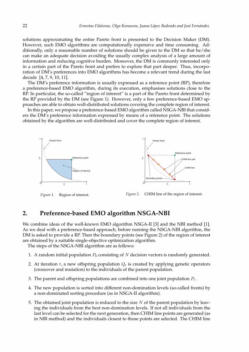
The DM’s preference information is usually expressed as a reference point (RP), thereforea preference-based EMO algorithm, during its execution, emphasises solutions close to theRP. In particular, the so-called “region of interest” is a part of the Pareto front determined bythe RP provided by the DM (see Figure 1). However, only a few preference-based EMO ap-proaches are able to obtain well-distributed solutions covering the complete region of interest.

In this paper, we propose a preference-based EMO algorithm called NSGA-NBI that consid-ers the DM’s preference information expressed by means of a reference point. The solutionsobtained by the algorithm are well-distributed and cover the complete region of interest.

f2

f1

Reference point

1

10

Region of interest

Pareto front

Figure 1. Region of interest.

f2

f1

Pareto front

Reference point

1

10

CHIM line

Boundary points

CHIM line poin

Figure 2. CHIM line of the region of interest.

2. Preference-based EMO algorithm NSGA-NBI

We combine ideas of the well-known EMO algorithm NSGA-II [3] and the NBI method [1].As we deal with a preference-based approach, before running the NSGA-NBI algorithm, theDM is asked to provide a RP. Then the boundary points (see Figure 2) of the region of interestare obtained by a suitable single-objective optimization algorithm.

The steps of the NSGA-NBI algorithm are as follows:

1. A random initial population P0 consisting of N decision vectors is randomly generated.

2. At iteration t, a new offspring population Qt is created by applying genetic operators(crossover and mutation) to the individuals of the parent population.

3. The parent and offspring populations are combined into one joint population Pt .

4. The new population is sorted into different non-domination levels (so-called fronts) bya non-dominated sorting procedure (as in NSGA-II algorithm).

5. The obtained joint population is reduced to the size N of the parent population by leav-ing the individuals from the best non-domination levels. If not all individuals from thelast level can be selected for the next generation, then CHIM line points are generated (asin NBI method) and the individuals closest to those points are selected. The CHIM line

Preference-Based Multi-Objective Evolutionary Algorithm 23

points are evenly distributed between the boundary points (see Figure 2). The numberof points on the CHIM line is equal to the number of points to be selected for the newpopulation from the last non-dominated level that cannot be completely selected.

6. If the termination condition is not satisfied, then the process is repeated from Step 2considering the reduced population as the parent population in the next iteration.

3. Results and conclusions

The proposed algorithm has been experimentally compared with a recently developed WAS-FGA algorithm [9] also designed to approximate the region of interest. The performance ofthe preference-based EMO algorithms has been evaluated using the following metrics: Gen-erational Distance (GD) [2] for estimating convergence to the true Pareto-front, Spread [2] forestimating the distribution evenness of the solutions, Hypervolume (HV) [13] for estimatingboth convergence and distribution. The new PR metric [5] is also considered – it evaluatesthe percentage of solutions that lie into the DM’s region of interest. The set of well-known2-objective test problems ZDT1–ZDT4, ZDT6 with different complexity and characteristics(convexity, concavity, discontinuity, non-uniformity, . . . ) has been considered [6].

Each algorithm has been run 30 times using different initial populations and average resultshave been evaluated. We selected a population size of 100 individuals and 100 generations.Those values are enough to obtain a good approximation of a region of the Pareto front inreasonable computational time.

Preference information provided by the DM that is expressed as a RP is required for theevaluated algorithms, therefore various RPs (achievable as well as unachievable) have beenselected. The used RPs, the numbers of objectives and variables for each test problem consid-ered are presented in Table 1.

We can see in Tables 2 and 3 that the proposed NSGA-NBI algorithm is superior in most ofthe cases (better values are marked in bold). In all the analysed cases, and according to the GDmetric, the proposed algorithm approximates the region of interest better than the WASFGAalgorithm. The values of Spread metric show that the solutions obtained by the NSGA-NBI al-gorithm are better evenly distributed in most of the cases. The proposed algorithm is superiorfor all analysed cases according to the HV metric. The PR metric indicates that the proposedalgorithm is able to obtain sufficiently high number of solutions in the region of interest forall analysed problems unlike the WASFGA algorithm. When solving the ZDT6 problem withachievable RP the WASFGA algorithm could not obtain any solutions in the region of inter-est, therefore the mean values of GD, Spread, and HV metrics could not be calculated – weshow these values as NaN (see Table 2). In conclusion, the proposed algorithm NSGA-NBI hasshown promising results, as it has obtained competitive values for all the quality indicatorsconsidered.

Table 1. Test problems and reference points used in the evaluated algorithms

Problem Number of Number of Achievable Unachievableobjectives variables reference point reference point

ZDT1 2 30 (0.80, 0.60) (0.20, 0.40)ZDT2 2 30 (0.80, 0.80) (0.50, 0.30)ZDT3 2 30 (0.30, 0.80) (0.05, 0.00)ZDT4 2 10 (0.80, 0.60) (0.08, 0.25)ZDT6 2 10 (0.78, 0.61) (0.39, 0.21)

24 Ernestas Filatovas, Olga Kurasova, Juana López Redondo and José Fernández

Table 2. Values of performance metrics for achievable RPs

GD Spread HV PRProblem NSGA-NBI WASFGA NSGA-NBI WASFGA NSGA-NBI WASFGA NSGA-NBI WASFGAZDT1 0.0004 0.0160 0.0049 0.0064 0.1760 0.1612 98.47 100.00ZDT2 0.0018 0.0344 0.0065 0.0331 0.0687 0.0513 98.17 95.97ZDT3 0.0005 0.0101 0.0062 0.0066 0.0689 0.0590 99.43 100.00ZDT4 0.0003 0.1345 0.0046 0.0202 0.1758 0.0649 98.57 55.50ZDT6 0.0004 NaN 0.0012 NaN 0.0162 NaN 98.87 0.00

Table 3. Values of performance metrics for unachievable RPs

GD Spread HV PRProblem NSGA-NBI WASFGA NSGA-NBI WASFGA NSGA-NBI WASFGA NSGA-NBI WASFGAZDT1 0.0003 0.0107 0.0047 0.0078 0.0127 0.0101 98.80 81.13ZDT2 0.0009 0.0214 0.0054 0.0066 0.0716 0.0592 97.44 80.20ZDT3 0.0006 0.0085 0.0207 0.0078 0.1150 0.1049 93.77 93.93ZDT4 0.1048 0.1938 0.1048 0.0520 0.2167 0.0411 88.83 36.43ZDT6 0.0002 0.1769 0.0017 0.0320 0.1354 0.0299 98.90 28.27

References

[1] Indraneel Das and John E. Dennis. Normal-boundary intersection: A new method for generating the paretosurface in nonlinear multicriteria optimization problems. SIAM Journal on Optimization, 8(3):631–657, 1998.

[2] Kalyanmoy Deb. Multi-objective Optimization using Evolutionary Algorithms. John Wiley & Sons, 2001.

[3] Kalyanmoy Deb, Amrit Pratap, Sameer Agarwal, and TAMT Meyarivan. A fast and elitist multiobjectivegenetic algorithm: NSGA-II. IEEE Transactions on Evolutionary Computation, 6(2):182–197, 2002.

[4] Kalyanmoy Deb, J. Sundar, N. Udaya Bhaskara Rao, and Shamik Chaudhuri. Reference point based multi-objective optimization using evolutionary algorithms. International Journal of Computational Intelligence Re-search, 2(3):273–286, 2006.

[5] Ernestas Filatovas, Algirdas Lancinskas, Olga Kurasova, and Julius Zilinskas. A preference-based multi-objective evolutionary algorithm R-NSGA-II with stochastic local search. Central European Journal of Opera-tions Research, Accepted.

[6] Simon Huband, Philip Hingston, Luigi Barone, and Lyndon While. A review of multiobjective test problemsand a scalable test problem toolkit. IEEE Transactions on Evolutionary Computation, 10(5):477–506, 2006.

[7] Antonio López-Jaimes and Carlos A. Coello Coello. Including preferences into a multiobjective evolutionaryalgorithm to deal with many-objective engineering optimization problems. Information Sciences, 277:1–20,2014.

[8] Kaisa Miettinen. Nonlinear Multiobjective Optimization. Springer, 1999.

[9] Ana Belén Ruiz, Rubén Saborido, and Mariano Luque. A preference-based evolutionary algorithm for mul-tiobjective optimization: the weighting achievement scalarizing function genetic algorithm. Journal of GlobalOptimization, pages 1–29, 2014.

[10] Florian Siegmund, Amos H.C. Ng, and Kalyanmoy Deb. Finding a preferred diverse set of Pareto-optimalsolutions for a limited number of function calls. In 2012 IEEE Congress on Evolutionary Computation (CEC),pages 1–8, 2012.

[11] Karthik Sindhya, Ana Belen Ruiz, and Kaisa Miettinen. A preference based interactive evolutionary al-gorithm for multi-objective optimization: PIE. In 6th International Conference on Evolutionary Multi-criterionOptimization, EMO 2011, pages 212–225. Springer, 2011.

[12] El-Ghazali Talbi. Metaheuristics: from Design to Implementation, volume 74. John Wiley & Sons, 2009.

[13] Eckart Zitzler and Lothar Thiele. Multiobjective optimization using evolutionary algorithms - a comparativecase study. In Parallel Problem Solving from Nature - PPSN V, pages 292–301. Springer, 1998.

Proceedings of GOW’16, pp. 25 – 28.

Energy-Aware Computation of EvolutionaryMulti-Objective Optimization∗

G. Ortega1, J.J. Moreno1, E. Filatovas2, J.A. Martínez1 and E.M. Garzón1

1Informatics Dpt., Agrifood Campus of International Excellence (ceiA3), University of Almería, Ctra. Sacramento s/n. LaCañada de San Urbano, 04120 Almería, Spain gloriaortega@ual.es, juanjonrg@gmail.com, jmartine@ual.es, gmartin@ual.es

2Vilnius University, Universiteto str. 3, Vilnius, Lithuania, Ernestas.Filatovas@mif.vu.lt

Abstract Large-scale multi-objective optimization problems with many criteria have a need for Ultrascalecomputing to solve them within a reasonable amount of time. Current evolutionary multi-objectiveoptimization algorithms as well as their parallel versions being designed for this goal do not con-sider energy consumption and savings – only the execution time is treated as main criterion of analgorithm efficiency.

In this research we focus on the most computationally expensive part of the state-of-the-art evo-lutionary NSGA-II algorithm – non-dominated sorting procedure – which consumes most of thecomputational burden. The impact of CPU and GPU workloads on power consumption and energyefficiency is experimentally investigated for our recently developed parallel versions of the FastNon-Dominated Sorting (FNDS) procedure when solving the multi-objective optimization prob-lems. Estimation of the balance between energy consumption and performance is also carried out,and the recommendation of usage of the developed parallel version of non-dominated sorting pro-cedure depending on the specific platform and architecture are provided as well. The results ofthis research will help to design the NSGA-II based energy aware algorithms for solving large-scalemulti-objective optimization problems.

Keywords: Multi-objective Optimization, Evolutionary Algorithms, NSGA-II, Green Computing,High-Performance Computing

1. Introduction

The main goal of Multi-Objective Optimization (MOO) is to provide the set of solutions thatdetermine the Pareto front. Due the complexity of the majority of MOO problems it is im-possible to obtain the exact Pareto front, therefore Evolutionary Multi-objective Optimization(EMO) algorithms are commonly-used to approximate the Pareto front [2, 15, 18]. There aremany works where EMO algorithms are successfully applied for solving relatively the smallmulti-objective optimization problems with small number of objectives, where the popula-tion size do not exceed 1,000 individuals. It is obvious that when the number of objectives in-creases very large populations should be used in EMO algorithms to represent the Pareto frontinformatively. However, is such cases computational load of the EMO algorithms strongly in-creases. Recently, several parallel versions of EMO algorithms have been developed, whichcan exploit the resources of Ultrascale computing platforms, with the unique goal of to im-prove the performance of these methods [9, 13, 14].

Nowadays, the energy efficiency is another target in several computational contexts. Specif-ically, in Ultrascale computation large data centres the energy consumption has a strong im-pact in the management cost and reliability. As consequence, an intensive effort is being de-veloped to design approaches for improving the energy/power efficiency of computational

∗This work has been partially supported by the Spanish Ministry of Science throughout project TIN15-66680, by J. Andalucíathrough projects P12-TIC-301 and P11-TIC7176, and by the European Regional Development Fund (ERDF)

26 G. Ortega, J.J. Moreno, E. Filatovas, J.A. Martínez and E.M. Garzón

devices and platforms [1, 7, 10, 12, 16]. Currently, energy costs represent a relevant share ofthe total costs of High Performance Computing (HPC) systems. They include several kindsof processing units, such as CPU cores and GPU, whose energy consumption depends on thekind of processing which is performing. The energy consumed by a computational processcan be get as the product of its run-time and the average electrical power during its execution.It plays a key role for evaluating the efficiency of the systems in terms of performance andpower/energy.

In this work we focus on development of energy-aware EMO algorithms. The majorityof the EMO approaches in the literature are based on Pareto dominance ranking, which iscomputed by a Non-Dominated Sorting (NDS) procedure [3, 4, 5, 8, 19], etc. As shown in [9,14], it consumes most of the computational burden of the EMO algorithm.

NSGA-II, as a representative EMO algorithm based on NDS procedure, is analysed in thiswork in terms of energy efficiency. We have developed three parallel versions of NSGA-IIwhich accelerate the NDS procedure on: (1) a multicore processor, (2) a GPU card and (3) both.Our main goal is to define the computational resources (number of cores and/or GPU) whatoptimize the energy efficiency. Therefore, for every combination platform-resources/problem-size the energy E is evaluated for a analysed test problem. The analysis of the results allowsus: (1) to evaluate the energy consumption of NSGA-II when it is computed on several com-putational resources and test problems and (2) to select appropriate resources of platforms tocompute NSGA-II, according to the number of individuals in the populations (N ), number ofobjective functions (M ) and number of CPU cores/ GPU cards of the available computationalplatforms. Therefore, this work results a methodology to optimize the energy consumption ofthe NSGA-II on platforms with several CPU cores and GPU cards.

2. Multi-objective optimization problems

A multi-objective minimization problem is formulated as follows [11]:

minx∈S

f(x) = [f1(x), f2(x), . . . , fM (x)]T (1)

where z = f(x) is an objective vector, defining the values for all objective functions f1(x), f2(x),. . . , fM (x), fi : RV → R, i ∈ 1, 2, . . . ,M, where M ≥ 2 is the number of objective func-tions; and x = (x1, x2, . . . , xV ) is a vector of variables (decision vector) and V is the number ofvariables S ⊂ RV is search space, which defines all feasible decision vectors.

A decision vector x′ ∈ S is a Pareto optimal solution if fi(x′) 6 fi(x) for all x ∈ S and fj(x′) <fj(x) for at most one j. Objective vectors are defined as optimal if none of their elements canbe improved without worsen at least one of the other elements. An objective vector f(x′) isPareto optimal if the corresponding decision vector x′ is Pareto optimal. The set of all thePareto optimal decision vectors is called the Pareto set. The region defined by all the objectivefunction values for the Pareto set points is called the Pareto front.

For two objective vectors z and z′, z′ dominates z (or z′ z) if z′i 6 zfi for all i = 1, . . . ,Mand there exists at most one j such that z′j < zj . In EMO algorithms, the subset of solutions in apopulation whose objective vectors are not dominated by any other objective vector is calledthe non-dominated set, and the objective vectors are called the non-dominated objective vectors.The main aim of the EMO algorithms is to generate well-distributed non-dominated objectivevectors as close as possible to the Pareto front.

NSGA-II [4] is the most widely-used and well-known EMO algorithm for approximatingthe Pareto front that is based on NDS. Thus, it is selected to analyse the energy efficiency ofEMO algorithms when different number of CPU cores and/or GPU cards are exploited.

The steps of NSGA-II are described in Algorithm 1. The Step 2 of the algorithm is devotedto the NDS procedure which is the most computationally expensive in the NSGA-II.

Energy-Aware Computation of EMO 27

Step 1: Generate a random initial population P0 of size N .Step 2: Sort the population to different non-domination levels (fronts) using, and assigneach individual a fitness equal to its non-domination level (1 is the best level).Step 3: Create an offspring population of size N using binary tournament selection,recombination and mutation operations (parents with larger crowding distance arepreferred if their non-domination levels are the same).Step 4: Combine the parent and the offspring populations and create a population R.Step 5: Reduce the population R to the population P of size N : sort the population Rinto different non-dominated fronts; fill the population P with individuals frompopulation R starting from the best non-dominated front until the size of P is equal to N ;if all the individuals in a front cannot be picked fully, calculate a crowding distance andadd individuals with the largest distances into the population P .Step 6: Check if the termination criterion is satisfied. If yes, go to Step 7, else return toStep 2.Step 7: Stop.

Algorithm 1: NSGA-II.

3. Energy efficiency evaluation of NSGA-II

In this section, a preliminary study of NSGA-II energy consumption is carried out. Thewidely-used DTLZ2 benchmark problem [6] has been considered as it suits well for experi-mental evaluation in this context. The test platform has been a Bullx R421-E4 Intel Xeon E52620v2 (12 CPU-cores, 64-GB RAM and 1-TB HDD) with a NVIDIA K80 (Kepler GK210) GPU.The NSGA-II algorithm has been implemented in MATLAB and it can call to several paral-lel NDS routines (multicore or GPU version). The multicore version is based on C++ andPthreads and the GPU version is developed on CUDA 7.5. All the test have been executedwith a number of generations equal to 100. The size of the population ranges from 200 to5,000. The power measurements on CPU (or GPU) have been sampled by an external monitorprogram that queries RAPL register using the PAPI library [17] (or NVML interface).

Figure 1. Runtime in seconds (left) and the consumed energy in KJ (right) when the NSGA-II is executed withseveral populations sizes (200, 500, 1,000, and 5,000) for solving the DTLZ2 problem on several resources of BullxR421-E4 Intel Xeon E5 2620v2 (12 CPU-cores) with a NVIDIA K80 GPU.

Figure 1 shows the runtime (in seconds) and the consumed energy (KJ) when the NSGA-II is executed with different population sizes solving the DTLZ2 problem with 5 objectivefunctions on several resources of the test computational platform (1-12 cores, 1GPU). As itcan be observed, the runtime and energy strongly increase with the size of the population.Moreover, runtime and energy vary with the selection of the resources. For instance, when thepopulation size is 5,000, the optimal execution is on the GPU in terms of energy consumption.

28 G. Ortega, J.J. Moreno, E. Filatovas, J.A. Martínez and E.M. Garzón

When the problem size is 500, the subset of 8 cores minimizes the energy consumption. So,for a specific platform (with a set of available resources) and several instances of problems ofthe NSGA-II algorithm, it is necessary to define approaches to identify what is the subset ofresources to optimize the energy consumption.

References

[1] J. Carretero, S. Distefano, D. Petcu, D. Pop, T. Rauber, G. Rünger, and D. Singh. Energy-efficient algorithmsfor ultrascale systems. Supercomputing frontiers and innovations, 2(2), 2015.

[2] K. Deb. Multi-objective Optimization using Evolutionary Algorithms. John Wiley & Sons, 2001.

[3] K. Deb and H. Jain. An improved NSGA-II procedure for many-objective optimization, Part I: Solvingproblems with box constraints. KanGAL Report, (2012009), 2012.

[4] K. Deb, A. Pratap, S. Agarwal, and T. Meyarivan. A fast and elitist multiobjective genetic algorithm: NSGA-II. IEEE Transactions on Evolutionary Computation, 6(2):182–197, 2002.

[5] K. Deb, J. Sundar, N. Udaya, and S. Chaudhuri. Reference point based multi-objective optimization usingevolutionary algorithms. International Journal of Computational Intelligence Research, 2(3):273–286, 2006.

[6] K. Deb, L. Thiele, M. Laumanns, and E. Zitzler. Scalable multi-objective optimization test problems. In IEEEWorld Congress on Computational Intelligence, pages 825–830, 2002.

[7] Y. Deng, Y. Hu, X. Meng, Y. Zhu, Z. Zhang, and J. Han. Predictively booting nodes to minimize performancedegradation of a power-aware web cluster. Cluster Computing, 17(4):1309–1322, 2014.

[8] E. Filatovas, O. Kurasova, and K. Sindhya. Synchronous R-NSGA-II: An Extended Preference-Based Evolu-tionary Algorithm for Multi-Objective Optimization. Informatica, 26(1):33–50, 2015.

[9] S. Gupta and G. Tan. A scalable parallel implementation of Evolutionary Algorithms for Multi-Objectiveoptimization on GPUs. In IEEE Congress on Evolutionary Computation, pages 1567–1574. IEEE, 2015.

[10] Y. Kang, W. Choi, B. Kim, and J. Kim. On tradeoff between the two compromise factors in assigning taskson a cluster computing. Cluster Computing, 17(3):861–870, 2014.

[11] K. Miettinen. Nonlinear Multiobjective Optimization, volume 12 of International Series in Operations Researchand Management Science. Kluwer Academic Publishers, Dordrecht, 1999.

[12] S. Mittal and J.S. Vetter. A Survey of Methods for Analyzing and Improving GPU Energy Efficiency. ACMComputing Surveys, 47(2):19:1–19:23, August 2014.

[13] D. Sharma and P. Collet. Implementation techniques for massively parallel multi-objective optimization. InMassively Parallel Evolutionary Computation on GPGPUs, pages 267–286. Springer, 2013.

[14] C. Smutnicki, J. Rudy, and D. Zelazny. Very fast non-dominated sorting. Decision Making in Manufacturingand Services, 8(1-2):13–23, 2014.

[15] E. Talbi. Metaheuristics: from Design to Implementation, volume 74. John Wiley & Sons, 2009.

[16] Y. Tian, C. Lin, and K. Li. Managing performance and power consumption tradeoff for multiple heteroge-neous servers in cloud computing. Cluster Computing, 17(3):943–955, 2014.

[17] V.M. Weaver, M. Johnson, K. Kasichayanula, J. Ralph, P. Luszczek, D. Terpstra, and S. Moore. MeasuringEnergy and Power with PAPI. In Proceedings of the 2012 41st International Conference on Parallel ProcessingWorkshops, ICPPW ’12, pages 262–268, Washington, DC, USA, 2012. IEEE Computer Society.

[18] Q. Zhang and H. Li. MOEA/D: A multiobjective evolutionary algorithm based on decomposition. IEEETransactions on Evolutionary Computation, 11(6):712–731, 2007.

[19] E. Zitzler, M. Laumanns, and L. Thiele. SPEA2: Improving the Strength Pareto Evolutionary Algorithm.Technical Report 103, Computer Engineering and Networks Laboratory (TIK), ETH Zurich, Zurich, Switzer-land, 2001.

Proceedings of GOW’16, pp. 29 – 32.

Locating a Facility with the Partially ProbabilisticChoice Rule∗

José Fernández1, Boglárka G.-Tóth2, Juana López Redondo3 and Pilar Martínez Ortigosa3

1University of Murcia, Murcia, Spainjosefdez@um.es

2Budapest University of Technology and Economics, Budapest, Hungarybog@math.bme.hu

3University of Almería, Agrifood Campus of International Excellence, ceiA3, Almería, Spainjlredondo,ortigosa@ual.es

Abstract Locating a facility is a strategic decision which usually requires a massive investment. In a com-petitive environment, where other facilities offering the same goods or products exist, the locationand quality of a facility may determine its success or failure. The profit that a facility obtains largelydepends on the market share that it captures, and this depends on the attraction that the customersfeel for the facility and on the patronizing behavior of the customers. In this work we assume thatthe former can be appropriately computed, and we concentrate on the latter. In this paper we con-sider that a customer only patronizes those facilities for which he/she feels an attraction greater thanor equal to a threshold value. Implicitly, this implies that there may be some unmet demand. Weapply this new rule to the problem of locating a single new facility in the plane, where the quality ofthe new facility to be located is also considered as a variable of the problem to be determined. Thethreshold value provokes discontinuities in the objective function of the problem. Both exact andheuristic methods are proposed to solve the location problem with the new choice rule.

Keywords: Continuous location, Competition, Customer choice rule, Interval branch-and-bound method, Pa-tronizing behavior, Evolutionary Algorithms, Computational study

1. Introduction

The patronizing behavior of customers is one of the core inputs in many business and eco-nomic indicators. This is the case for the estimation of the market share captured by thefacilities in a competitive environment. When there exist several facilities offering the sameproduct, the way in which customers decide to spend their buying power among them maydetermine the success or the failure of the facilities. Consumer behavior is a function of theattraction that consumers feel for the facilities. This attraction is the result of several factors,but the two most important forces are the location of the facilities and their quality: the closerthe facility to the customer and the higher its quality, the greater the attraction of the customertowards the facility. In fact, when a company wants to enter a market or to expand its presenceby opening new facilities, both the location and the quality of the new facilities are chosen soas to maximize the revenues obtained by the chain, which largely depend on the market sharethat it captures.

∗This research has been supported by grants from the Spanish Ministry of Economy and Competitiveness (MTM2015-70260-P,TIN2015-66680-C2-1-R), Fundación Séneca (The Agency of Science and Technology of the Region of Murcia, 19241/PI/14), Juntade Andalucía ( P11-TIC7176 and P12-TIC301 ), in part financed by the European Regional Development Fund (ERDF). This workis also funded by the Hungarian National Research, Development and Innovation Office âAS NKFIH, OTKA grant PD115554and also by the project ICT COST Action TD1207 (EU). Juana López Redondo is a fellow of the Spanish ‘Ramón y Cajal’ contractprogram.

30 José Fernández, Boglárka G.-Tóth, Juana López Redondo and Pilar Martínez Ortigosa

The new customer choice rule introduced here is an extension of the classical probabilisticchoice rule. According to the new rule, called partially probabilistic choice rule, a customer,in order to satisfy his/her demand, only patronizes those facilities for which he/she feels anattraction greater than or equal to a threshold value, and the demand is split among them pro-portionally to their attraction. employed in literature, the threshold value implicitly impliesthat there may be some unmet demand.

The influence of the choice rule in the location of competitive facilities has been analyzed.In particular, the problem of locating a single new facility in the plane has been considered.The corresponding location problem for profit maximization has been formulated, and anexact interval branch-and-bound method (iB&B), as well as a heuristic evolutionary algorithm(UEGO) have been proposed to cope with the problem.

2. The partially probabilistic location problem

We will assume the following particular scenario (see [1] for more details). A single newfacility is going to be located in a given region of the plane by a chain. There already existm facilities around selling the same goods or product; k of those facilities may belong to thelocating chain. The demand to be served, known and fixed, is concentrated at some demandpoints, whose locations are known. The location and quality of the existing facilities is alsoknown. The attraction function of a demand point towards a facility is modeled as perceivedquality divided by perceived distance. The maximization of the profit obtained by the chainafter the location of the new facility is the objective to be achieved, to be understood as theincome due to the market share captured by the chain minus its operational costs. The aim isto find both the location and the quality of the new facility to be located.

It is important to have effective methods for solving the location problems. Usually com-petitive location problems lead to hard-to-solve global optimization problems. The challengeof the location problem with the partially probabilistic choice rule is that it also presents dis-continuities as a consequence of the threshold value (see Figure 1). For the problem at hand,the usefulness of the interval branch-and-bound algorithm iB&B [1] and the evolutionary al-gorithm UEGO [5, 6] has been investigated.

0.5 1 1.5 2 2.5 3 3.5 4 4.5 5 5.5125

130

135

140

145

150

155

160

165

Figure 1. Projections of the objective function of an instance with setting (imax = 71, jmax = 5, k = 2) when thethreshold value is equal to 2. On the left, when α = 1.545898. On the right, when (x1 = 3.989257, x2 = 7.065429)

Interval B&B methods have been successfully applied to solve other location problems (seefor instance [2, 8] and the references therein). In particular, in [1] such a method was appliedto solve the corresponding probabilistic problem. A similar method can handle the partiallyprobabilistic model, thanks to the use of the interval tools employed to compute the bounds.However, only the discarding tests described in [1] which do not make use of the differentia-

Locating a Facility with the Partially Probabilistic Choice Rule 31

Table 1. UEGO results for problems with n = 10000 demand points.

(m, k)prob Time Distance Minimum Average Maximum Deviation(100, 25)1 763.1 0.010 14026.9 14026.9 14026.9 0.006(100, 25)2 631.9 0.006 13059.7 13059.7 13059.7 0.012(100, 25)3 629.2 0.046 14092.3 14092.4 14092.4 0.043(100, 25)4 480.3 0.145 15650.1 15650.4 15650.6 0.165(100, 25)5 534.0 0.002 12688.1 12688.1 12688.1 0.013average 607.7 0.042 13903.4 13903.5 13903.5 0.048(100, 50)1 729.4 0.002 24672.3 24672.3 24672.3 0.000(100, 50)2 857.6 0.009 27241.9 27241.9 27241.9 0.012(100, 50)3 435.3 0.010 27092.0 27092.1 27092.1 0.038(100, 50)4 678.0 0.081 24517.4 24517.4 24517.4 0.013(100, 50)5 837.9 0.000 29174.6 29174.6 29174.6 0.002average 707.6 0.020 26539.6 26539.6 26539.7 0.013(200, 50)1 527.3 0.000 12684.2 12684.2 12684.2 0.000(200, 50)2 660.7 0.051 12102.1 12102.3 12102.3 0.074(200, 50)3 679.8 0.108 12447.8 12447.9 12448.0 0.072(200, 50)4 529.6 0.220 12572.6 12572.8 12572.9 0.110(200, 50)5 691.1 0.105 14112.2 14112.2 14112.3 0.051average 617.7 0.097 12783.8 12783.9 12784.0 0.061(200, 100)1 903.4 0.098 25274.8 25274.8 25274.9 0.007(200, 100)2 912.4 0.128 26845.2 26845.2 26845.3 0.037(200, 100)3 884.9 0.000 24426.4 24426.4 24426.4 0.000(200, 100)4 626.4 0.003 23853.1 23853.1 23853.1 0.001(200, 100)5 594.2 0.059 27100.8 27100.8 27100.9 0.015average 784.3 0.058 25500.1 25500.1 25500.1 0.012

bility of the objective function can be used for the new problem, namely, the cut-off and thefeasibility tests. In addition to this, inclusion functions for piece-wise functions have had tobe designed.

UEGO is a general heuristic able to solve many global optimization problems. In fact, it hasalso been applied to other competitive location problems as well (see for instance [4]). Only thelocal search procedure used within UEGO needs to be adapted for each particular problem.In view of its success in solving different competitive location problems, UEGO has also beenadapted to the problem with the partially probabilistic choice rule. It was first implementedusing a Weiszfeld-like algorithm as a local search, following the lines in [5]. However, theobtained results were not as good as expected. It is with the stochastic hill climber SASS [7]that UEGO can solve the problem effectively and efficiently as we will see. The use of SASSas the local optimizer within UEGO has also worked fine for other location problems withdiscontinuities (see for instance [3]).

3. Computational results

A comprehensive computational study has been carried out. In all, 80 problems have beensolved, i.e., 20 instances for 4 different number of demand points n =500, 1000, 5000 and10000.

The exact iB&B can manage instances with up to 1000 demand points without difficulties,but it starts experiencing problems with instances with 5000 demand points. This clearlyshows the difficulty of the problem at hand, and the need for a heuristic method to copewith large-size problems. Regarding UEGO, it is quite robust. It has 100% success in all theproblems solved by iB&B, i.e, in all the problems and in all the runs, the solution providedby UEGO was always included in one of the solution boxes provided by iB&B. In fact, theminimum, average and maximum objective function values obtained by UEGO are always

32 José Fernández, Boglárka G.-Tóth, Juana López Redondo and Pilar Martínez Ortigosa

about the same. Not only is the objective function value the same in all the runs, but thesolution point offered by the algorithm is also the same. And this using a tiny fraction of theCPU time employed by iB&B.

On the other hand, UEGO is a reliable heuristic method, able to solve problems with up to10000 demand points without difficulties, solving them in less than 13 minutes. Table 1 showsthe results obtained by UEGO for the 20 instances with 1000 demand points and differentvalues for m and k. The actual settings employed can be seen in Table 1. Notice that UEGOis a stochastic algorithm, and hence each run may lead to a different solution. To take thisfact into account, each problem has been solved 5 times, and the following values have beencomputed: the average CPU time employed in solving the problem in the 5 runs, the maxi-mum Euclidean distance between any pair of solutions, the minimum, average and maximumobjective function values of the solutions and the corresponding standard deviation.

4. Summary

In this work, a new location problem is studied. It has been solved by means of an intervalBranch & Bound method and an evolutionary algorithm. From the computational study, it canbe concluded that iB&B can solve problems with up to 1000 demand points exactly. For largerinstances, the use of the evolutionary algorithm UEGO is recommended, as it is a reliable androbust method.

References

[1] J. Fernández, B. Pelegrín, F. Plastria, and B. Tóth. Solving a Huff-like competitive location and design modelfor profit maximization in the plane. European Journal of Operational Research, 179(3):1274–1287, 2007.

[2] J. Fernández and B. Pelegrín. Using interval analysis for solving planar single-facility location problems: newdiscarding tests. Journal of Global Optimization, 19(1):61–81, 2001.

[3] J.L. Redondo, J. Fernández, A.G. Arrondo, I. García, and P.M. Ortigosa. A two-level evolutionary algorithmfor solving the facility location and design (1|1)-centroid problem on the plane with variable demand. Journalof Global Optimization, 56(3):983–1005, 2013.

[4] J.L. Redondo, J. Fernández, A.G. Arrondo, I. García, and P.M. Ortigosa. Fixed or variable demand? Does itmatter when locating a facility? Omega, 40(1):9–20, 2012.

[5] J.L. Redondo, J. Fernández, I. García, and P.M. Ortigosa. A robust and efficient global optimization algorithmfor planar competitive location problems. Annals of Operations Research, 167(1):87–106, 2009.

[6] J.L. Redondo, J. Fernández, I. García, and P.M. Ortigosa. Parallel algorithms for continuous competitive loca-tion problems. Optimization Methods & Software, 23(5):779–791, 2008.

[7] F.J. Solis and R.J.B. Wets. Minimization by random search techniques. Mathematics of Operations Research,6(1):19–30, 1981.

[8] B. Tóth and J. Fernández. Interval methods for single and bi-objective optimization problems - applied to competitivefacility location problems. Lambert Academic Publishing, Saarbrücken, 2010.

Proceedings of GOW’16, pp. 33 – 36.

On Regular Refinement of Unit Simplex byjust Visiting Grid Points∗

L.G. Casado1, J.M.G. Salmerón1, B.G.-Tóth2, E.M.T. Hendrix3 and I. García3

1University of Almería, Spain, leo@ual.es, josemanuel@ual.es

2Budapest University of Technology and Economics, Hungary, bog@math.bme.hu

3Universidad de Málaga, Spain, eligius@uma.es, igarciaf@uma.es

Abstract In Branch and Bound (BnB) algorithms, the branching rule plays an important rule in order to reducethe number of evaluated sub-problems and points. Recent studies addressed the unit simplex refine-ment with regular simplices. When the achieved accuracy is related on the distance among sampledpoints, a common method is to stop the refinement when the size of a sub-problem, measured asthe largest distance among its evaluated vertices, is smaller or equal to a given precision. The worstcase was studied: the complete tree is generated, which is determined by the size of its leafs. In suchscenario, 2USC (two-uniform-simplex cover) on a mesh grid showed a better performance than LEB(longest edge bisection) in terms of number of simplices and vertices evaluations. Due to the over-lapping of sub-simplices, termination criterion in 2USC can be relaxed but the largest precision tocover the mesh grid depends on the dimension. This work focus on the study of the 2MUSC divisionmethod, where regular sub-simplices may have different orientation, in order to know if 2MUSC cancover the mesh grid for larger precisions than 2USC does.

Keywords: Unit simplex, Refinement Regular division, Mesh grid.

1. Introduction

The unit simplex is defined as

S1 = x ∈ Rd |d∑j=1

xj = 1; xj ≥ 0, ∀j. (1)

This search region is widely used for mixture design problems, equilibria and fixed pointproblems with application in economy, game theory and nonlinear systems of equations [10],co-positivity detection of matrices [1], stability in biological population dynamics [9] and oth-ers [7]. We studied these problems with quadratic constraints for practical mixture design inlubricant industry [6] and for the design of fat blends in food production [3, 5].

The main question is how to design a refinement strategy for a unit simplex such that thenumber of evaluated sub-problems and vertices is minimized taking explicitly the equidistantgrid with relative mesh size α into account. The size of a sub-problem is defined as w(S), thatis the width of the simplex S defined as the length of its longest edge. We assume a usergiven relative accuracy ε. A sub-problem S is not further divided when w(S) ≤ εw(S1). TheBnB algorithm returns the set of final and not rejected sub-problems. In this way, the problemsolution is guaranteed to be in one of the final sub-simplices with a size less than εw(S1).

Two points x, y on the α-grid over the unit simplex are neighbour if ∃i, j, i 6= j such that,yi = xi + α, yj = xj − α and yk = xk, for k 6= i, j. It is a challenge to find a refinement in

∗This work has been funded by grant from the Spanish Ministry (TIN2015-66688), Junta de Andalucía (P11-TIC-7176) and inpart financed by the European Regional Development Fund (ERDF).

34 L.G. Casado, J.M.G. Salmerón, B.G.-Tóth, E.M.T. Hendrix and I. García

the BnB algorithm that only generates sample points as vertices of the sub-sets that coincidewith grid points on S1. Given an accuracy ε, the largest value for the mesh size is α = 1

G ,with G = d1

ε e parts on each axis and G+ 1 grid point per axis, whereas two of them representvertices of S1. For the unit simplex, the number of α-grid points is given by [3]:

d−1∑k=1

(G+ 1k

)(d− 2k − 1

). (2)

According to [2], one can take the α mesh size to guide the refinement using regular simplicesof same size and orientation (2USC) and the improvement in the number of evaluated sub-problems and vertices is significant when is compared to longest edge bisection (LEB). Thedrawback of the 2USC refinement on the grid is that the smallest G value of the accuracyneeded to completely visit the grid depends on the dimension. This work studies the 2MUSC(2 Mixed Unit Simplex Cover) refinement of the unit simplex which uses the so-called 2USCand 2∇USC refinement, see [4]. 2∇USC generates regular sub-simplices of different size andorientation on the grid.

2. 2USC on grid

The two-uniform-simplex-cover refines a regular simplex in d overlapping regular sub-sim-plices with two sub-simplices per edge (see Figures 1 and 2). A reduction factor β ≥ d−1

dguarantees the covering of the refined simplex. Considering that sub-simplices overlap, therefinement method only evaluates an overlapped region once, see [4].

Figure 1. 2USC in R3. Dots represent the verticesand the centre of a sub-simplex.

Figure 2. 2USC in R4.

The main characteristics of the 2USC on α-grid are the following:

Let S` be a sub-simplex leaf of the d-ary tree. The general termination criterion w(S) ≤εw(S1) can be relaxed to w(S`) = α(d− 1)w(S1) ≤ εw(S1).

Regular Refinement of Unit Simplex 35

The sequence of sub-simplex size αki on each level i of the tree can be determined takinginto account that the size of every sub-simplex should be a multiple of α:

w(S1 = S0) = αk0 k0 = G

w(S1) = αk1, k1 =

⌈k0d− 1

d

⌉w(S2) = αk2, k2 =

⌈k1d− 1

d

⌉. . .

w(S`−2) = αk`−2, k`−2 =

⌈k`−3

d− 1

d

⌉w(S`−1) = αk`−1, k`−1 = d =

⌈k`−2

d− 1

d

⌉w(S`) = αk`, k` = d− 1 =

⌈k`−1

d− 1

d

⌉.

(3)

The minimum G value to force covering of the α-grid by the set of generated vertices in2USC refinement depends on the dimension d: G ≥ (d− 1)2.

3. 2MUSC on grid

2-mixed-uniform-simplex-cover refinement (2MUSC) combining 2USC and 2∇USC in the re-finement of the unit simplex. The 2∇-uniform-simplex-cover (2∇USC) introduced in [4] re-fines a regular simplex in d+ 1 regular sub-simplices. In contrast to 2USC, d of them have thesame orientation using a reduction factor d−2

d−1 ≤ ρ < d−1d and one non-overlapped inverted

sub-simplex has a reduction factor % = d(1− ρ)− 1. Figure 3 shows an example of 2∇USC ford = 3, where ρ = % = 1/2. Figure 4 shows an example for d = 4 where ρ = 2/3 and % = 1/3.

Figure 3. 2∇USC and α-grid with G = 2 and d =3. Big boxes are α-grid points and little boxes arevertices of simplices.

Figure 4. 2∇USC for d = 4.

In 2∇USC, the sub-simplices overlap less than in 2USC, but the sub-simplices are not equallyoriented and sized. 2∇USC requires a delicate choice of the reduction factor ρ. In order to havea value for ρ being a multiple of α, ρ should be greater or equal to (d − 1)/d. In that case, thereduction factor of the inverted simplex % ≤ 0. This means that the inverted sub-simplex doesnot exist and 2∇USC reduces to 2USC. Therefore, 2MUSC uses 2USC or 2∇USC dependingon the current simplex, either a reduction factor ρ or β is applied to force vertices of the gen-erated sub-simplices to be on the α-grid. The main characteristics of the 2MUSC on α-grid arethe following:

Assuming that last refinement is 2∇USC, the termination criterion can be relaxed tow(S`) = α(d− 2)w(S1).

36 L.G. Casado, J.M.G. Salmerón, B.G.-Tóth, E.M.T. Hendrix and I. García

The sequence of sub-simplex size αri on each level i of the tree are determined by:

w(S0) = αr0 r0 = G

w(S1) = αr1, r1 =

⌈r0d− 2

d− 1

⌉2∇USC, if

⌈r0d−2d−1

⌉< r0

d−1d

2USC, otherwise.

w(S2) = αr2, r2 =

⌈r1d− 2

d− 1

⌉2∇USC, if

⌈r1d−2d−1

⌉< r1

d−1d

2USC, otherwise.

. . .

w(Sl−1) = αrl−1, rl−1 =

⌈rl−2

d− 2

d− 1

⌉2∇USC, if

⌈rl−2

d−2d−1

⌉< rl−2

d−1d

2USC, otherwise.

w(Sl) = αrl, rl =

⌈rl−1

d− 2

d− 1

⌉(2∇USC),

(4)

where rl−1 = d− 1 and rl = d− 2.Due to the existence of different sequences depending on d andG, the minimumG valueto force covering of the α-grid has still to be determined.

4. Conclusions

This paper presentes the 2MUSC on grid refinement for the unit simplex, with less overlapthan 2USC on grid. Numerical results and the minimum number of segments G per axis tocover the α-grid will be outlined at GOW’16. The evaluation of these refinement methods fora real problem on a BnB algorithm will be also discussed in GOW’16 [8].

References

[1] Immanuel M. Bomze. On standard quadratic optimization problems. Journal of Global Optimization,13(4):369–387, 1998.

[2] L. G. Casado, E. M. T. Hendrix, J.M.G. Salmerón, B. G.-Tóth, and I. García. On grid aware refinement inbranch and bound. Submitted to Journal of Global Optimization.

[3] Leocadio G. Casado, Eligius M. T. Hendrix, and Inmaculada García. Infeasibility spheres for finding robustsolutions of blending problems with quadratic constraints. Journal of Global Optimization, 39(2):215–236, 2007.

[4] B. G.-Tóth, E. M. T. Hendrix, L. G. Casado, and I. García. On refinement of the unit simplex using regularsimplices. Journal of Global Optimization, 64(2):305–323, 2015.

[5] Eligius M. T. Hendrix, Leocadio G. Casado, and Inmaculada García. The semi-continuous quadratic mix-ture design problem: Description and branch-and-bound approach. European Journal of Operational Research,191(3):803 – 815, 2008.

[6] E.M.T. Hendrix and J. Pintér. An application of Lipschitzian global optimization to product design. Journalof Global Optimization, 1:389–401, 1991.

[7] E. de Klerk, D. den Hertog, and G Elabwabi. On the complexity of optimization over the standard simplex.European Journal of Operational Research, 191(3):773–785, 2008.

[8] J.M.G. Salmerón, L. G. Casado, E. M. T. Hendrix, and J.F.R. Herrera. On regular simplex division in solvingblending problems. In Proceedings of GOW’16: XIII Global Optimization Workshop, 2016.

[9] G. J. Still and F. Ahmed. Quadratic maximization on the unit simplex: structure, stability, genericity andapplication in biology. Memorandum 2034, Department of Applied Mathematics, University of Twente,Enschede, February 2014.

[10] Zaifu Yang. Computing Equilibria and Fixed Points, volume 21 of Theory and Decision Library C. Springer, 1999.

Proceedings of GOW’16, pp. 37 – 40.

Metabolic Pathway Analysis Using Nash Equilibrium

Angelo Lucia1 and Peter A. DiMaggio2

1Department of Chemical Engineering, University of Rhode Island, Kingston, RI 02881, USA, lucia@egr.uri.edu

2Department of Chemical Engineering, Imperial College London, London SW7 2AZ, UK, p.dimaggio@imperial.ac.uk

Abstract A novel approach to metabolic network analysis using a Nash equilibrium formulation is proposed.Enzymes are considered to be players in a multi-player game in which each player attempts to min-imize the dimensionless Gibbs free energy associated with the biochemical reaction(s) it catalyzessubject to elemental mass balances. Mathematical formulation of the metabolic network as a setof nonlinear programming (NLP) sub-problems and an appropriate solution methodologies are de-scribed. A small example representing part of the production cycle for acetyl-CoA is used to demon-strate the efficacy of the proposed Nash equilibrium framework and that it represents a paradigmshift in metabolic network analysis.

Keywords: Metabolic pathway analysis, Nash equilibrium, Global optimization

1. Introduction

Flux balance analysis (FBA) has been the mainstay for understanding and quantifying meta-bolic networks for many years. See, for example, [1, 2, 3, 4, 5, 6], and others. The basic ideabehind FBA is to represent a given metabolic network at steady-state in the form of a graphwith nodes that define specific biochemical reactions and fluxes that connect nodes. The con-straints for the network constitute a set of under-determined steady-state linear mass balanceequations. To complete the representation, a linear objective function relevant to the particu-lar biological task at hand (e.g., maximizing the output flux [5]; minimizing the cardinality ofthe flux vector [4]; minimum nutrient intake; minimum ATP production minimal knockout,etc.) is selected, which together with the mass balance constraints, results in a linear pro-gramming (LP) formulation. Many variants and extensions to FBA have also been proposedover the years, including Mixed Integer Linear Programming (MILP) formulations [7], theincorporation of linearized thermodynamic constraints [8] or thermodynamic metabolic fluxanalysis (TMFA), dynamic FBA [9], and others. In addition to FBA, the other main approachto metabolic network analysis involves a time-dependent or dynamic formulation that incor-porates chemical reaction kinetics.

Both the kinetic model and FBA approaches suffer from a number of significant modelingand biological limitations. For example, kinetic models require a large number of parametersthat are not ‘directly’ measurable and thus must be determined by model regression. Also, allFBA-based approaches are constrained only by reaction stoichiometry, which often results indegenerate solutions that lie on the user-specified flux bounds. Additional modeling limita-tions stem from the inability of either approach to accurately capture the inherent complex-ities within a crowded cellular environment. In particular, natural competition/cooperationamong enzymes exists for the pool of continuously produced metabolites and neither ap-proach takes into consideration the population distribution and/or heterogeneity of protein-metabolite interactions that form the basis for these reactions. Moreover, from a biologicalperspective, these approaches also fail to model the phenotypic consequence of overproduc-ing a given product and the subsequent regulation of overproduction in these organisms. For

38 Angelo Lucia and Peter A. DiMaggio

instance, it is well known that excess quantities of a given protein or small molecule can leadto ‘higher order’ interactions, which can be non-specific or the result of adaptive evolutionarypressures that activate alternative pathways to deplete these excess pools.

2. Nash Equilibrium Approach

This paper takes a radically different approach to metabolic network analysis by formulat-ing the problem as a Nash Equilibrium (NE) problem using first principles (i.e., conservationof mass and rigorous reaction thermodynamics). The key idea behind our proposed NE ap-proach is to view enzymes as ‘players’ in a multi-player game, in which each enzyme pursuesa strategy that can be quantified using a payoff or objective function. More specifically, thegoal of each enzyme is to minimize the dimensionless Gibbs free energy of the biochemicalreaction it catalyzes subject to appropriate elemental mass balances (i.e., conservation of massof carbon, hydrogen, oxygen, nitrogen, phosphorous, sulfur, etc.). Thus the overall goal of thenetwork is to find the best value of

G(v)

RT= min

N∑j=1

Gj(vj)

RT(1)

where GjRT , the dimensionless Gibbs free energy, is the objective function associated with the

appropriate enzymes involved in a particular set (or number) of metabolic reactions at a givennode j in the network, v is a vector of unknown metabolic fluxes, R is the gas constant andT is the temperature. The solution, called a NE point, optimizes the ’payoff’ of all playerssimultaneously, is the best solution for all players taken together, and not necessarily best forany one player. This NE approach, in our opinion, is a more accurate representation of theevolutionary-defined competition/cooperation observed in complex metabolic pathways.

Let the unknown variables, v, be partitioned into N subsets, v = [v1, v2, ..., vN ]. Each variablepartition, vj , has nj unknown variables and there are N total unknowns. The Nash Equi-librium formulation for an arbitrary metabolic network is different from that for FBA and isgiven by j = 1, 2, ..., N nonlinear programming (NLP) sub-problems of the form:

minGj(vj ,v

∗j )

RT (2)subject to conservation of mass

v∗j

The conservation of mass constraints are elemental mass balances and represent the flow ofmetabolic material in and out of any node. Finally, the vector, v∗j , denotes the minima of allother sub-problems, k = 1, 2, .., j − 1, j + 1, ..., N . In this article the words “sub-problem” and“node” mean the same thing.

3. Example

Figure 1 is a simplified metabolic network for the production of acetyl-CoA whose Nash Equi-librium formulation and solution were determined by specifying the input flux to the network(i.e., the pyruvate flux) and breaking the acetate feedback to the acetyl-CoA pool. Initial es-timates of the acetate flux and co-enzyme A (CoA) allows the NLP sub-problems associatedwith the following bio-chemical reaction equilibria to be solved in the order shown below.

1. Acetyl-CoA production from pyruvate and acetate:

C3H3O3 + C2H3O2 + 2C21H32N7O16P3S 2C23H34N7O17P3S + CO2 + H2O

NE Approach for Metabolic Pathway Analysis 39

D-Glucose

Gl col s sP t way Lactate

FormatePEP

Pyruvate

Acetylaldehyde Ethanol

Figure 1. Simplified metabolic network for the production of acetyl-CoA based on the iJO1366 E. coli network[10].

2. Acetyl phosphate production from acetyl-CoA:

C23H34N7O17P3S + HO4P C2H3O5P + C21H32N7O16P3S

3. Acetate production from acetyl phosphate:

C2H3O5P C2H3O−2 + PO3−

3

The solution of the acetate biochemical equilibrium provides new values for the acetate andCoA fluxes, which are compared to their initial estimates. If the initial and calculated valuesdo not match, the calculated values are used for the next iteration, and this process is repeateduntil convergence is achieved.

Table 1 gives a complete summary of the NE iterations and solution per nmol/h of pyruvatestarting from an initial estimate of acetate flux of vac = 1 nmol/h and stoichiometric CoA.Note that the NE iterations converge linearly and, after the first iteration, maintain a mono-tonically decreasing sequence of values of G/RT . In addition, the numerical results clearlyreveal that the objective function, G/RT , drives the solution to one that is best for the en-zymes lpd, acs, and aldB but not best for the enzyme pta. Table 2 presents a comparison ofthe NE predicted relative fluxes for the network and shows that the calculated results are infair agreement with available experimental data [11].

4. Summary

A Nash Equilibrium approach to metabolic pathway analysis was proposed. The key idea be-hind this approach is to view enzymes as players in a multi-player game, where each playeroptimizes a specific objective function. A small proof-of-concept example consisting of a sim-plified network for the production of acetyl-CoA with four players was presented. Predictedfluxes at the NE point were found to compare favorably with existing experimental data.

40 Angelo Lucia and Peter A. DiMaggio

Table 1. Nash Equilibrium Iterates and Solution to Acetyl-CoA Production.

Iter. G/RT ∗ vactp vac vPO3 vaccoa vcoa vpi vco2 vh2o Error

1 -12.48 0.0348 0.0844 0.0844 0.4330 1.5670 0.4330 0.5143 1.0380 0.91552 -12.30 0.0952 0.6787 0.1269 0.5889 1.4111 0.3303 0.8707 0.9403 0.59423 -14.34 0.1262 0.9593 0.1653 0.7754 1.2246 0.2608 1.1221 0.9449 0.28064 -15.46 0.1456 1.1275 0.1897 0.8792 1.1208 0.2171 1.2684 0.9461 0.16825 -16.07 0.1564 1.2223 0.2032 0.9380 1.0620 0.1927 1.3509 0.9467 0.09486 -16.39 0.1621 1.2752 0.2104 0.9704 1.0296 0.1799 1.3963 0.9465 0.05297 -16.57 0.1651 1.3045 0.2140 0.9879 1.0121 0.1732 1.4210 0.9460 0.02938 -16.67 0.1667 1.3206 0.2159 0.9972 1.0028 0.1698 1.4342 0.9456 0.01619 -16.72 0.1675 1.3294 0.2168 1.0022 0.9978 0.1680 1.4413 0.9452 0.008810 -16.74 0.1679 1.3341 0.2173 1.0048 0.9952 0.1671 1.4451 0.9450 0.004711 -16.76 0.1681 1.3367 0.2176 1.0063 0.9937 0.1666 1.4471 0.9448 0.002612 -16.77 0.1683 1.3381 0.2177 1.0070 0.9930 0.1664 1.4482 0.9448 0.001413 -16.77 0.1683 1.3388 0.2178 1.0074 0.9926 0.1662 1.4488 0.9447 0.0007

∗G/RT = min∑3j=1Gj/RT

Table 2. Comparison of Relative Flux Values Between Experimental Data [11] and Predictions using NE Model(Table 1).

Component Experimentally Measured Fluxes NE Predicted Fluxes

Acetyl-CoA 0.5443 0.4006Acetyl phosphate 0.0000 0.0669Acetate 0.4557 0.5324

References

[1] A. Varma and B.O. Palsson. Metabolic flux balancing: basic concepts, scientific and practical use. NatureBiotechnology, 12:994–998, 1994.

[2] K.J. Kauffman, P. Prakash, and J.S. Edwards. Advances in flux balance analysis. Current Opinions in Biotech-nology, 14:491–496, 2003.

[3] H.G. Holzhutter. The principles of flux minimization and its application to estimate stationary fluxes inmetabolic networks. European Journal of Biochemistry, 271:2905–2922, 2004.

[4] A.A. Julius, M. Imielinski, and G.J. Pappas. Metabolic networks analysis using convex optimization. InProceedings of the 47th IEEE Conference on Decision and Control, page 762, 2008.

[5] K. Smallbone and E. Simeonidis. Flux balance analysis: a geometric perspective. Journal of Theoretical Biology,258:311–315, 2009.

[6] E. Murabito, E. Simeonidis, K. Smallbone, and J. Swinton. Capturing the essence of a metabolic network: aflux balance analysis approach. Journal of Theoretical Biology, 260(3):445–452, 2009.

[7] S. Lee, C. Phalakornkule, M.M. Domach, and I.E. Grossmann. Recursive milp model for finding all thealternate optima in lp models for metabolic networks. Computers & Chemical Engineering, 24:711–716, 2000.

[8] C.S. Henry, L.J. Broadbelt, and V. Hatzimanikatis. Thermodynamic metabolic flux analysis. BiophysicalJournal, 92:1792–1805, 2007.

[9] R. Mahadevan, J.S. Edwards, and F.J. Doyle. Dynamic flux balance analysis in diauxic growth in escherichiacoli. Biophysical Journal, 83:1331–1340, 2002.

[10] J.D. Orth, T.M. Conrad, J. Na, J.A. Lerman, H. Nam, A.M. Feist, and B.O. Palsson. A comprehensive genome-scale reconstruction of escherichia coli metabolism–2011. Molecular Systems Biology, 11(7):535, 2011. doi:10.1038/msb.2011.65.

[11] H. Holms. Flux analysis and control of the central metabolic pathways in escherichia coli. FEMS MicrobiologyReview, 19:85–116, 1996.

Proceedings of GOW’16, pp. 41 – 44.

On Metaheuristics for Longest Edge Bisectionof the Unit Simplex to Minimise the Search Tree Size ∗

J.M.G. Salmerón1, J.L. Redondo1, E.M.T. Hendrix2 and L.G. Casado1

1Dept. Informatics, University of Almería (CeiA3), Spain, josemanuel,jlredondo,leo@ual.es

2Dept. Computer Architecture, University of Málaga, Spain, eligius@uma.es

Abstract In several areas like Global Optimization using branch-and-bound (B&B) methods for mixture de-sign, the unit n-simplex is refined by longest edge bisection. This process provides a binary searchtree. For n > 2, simplices appearing during the refinement process can have more than one LongestEdge (LE). The size of the resulting binary tree depends on the specific sequence of bisected longestedges. The question is how to choose the LE to bisect. In a previous work, a set of LE indices gener-ating the minimum number tree size was presented for n = 3 under the so-calledmk-valid conditionby means of a deterministic method that examined the whole set of minimum Binary Trees (BTs). Weare interested in find out new sets of rules for dimensions higher than 3. However, full enumerationof all possibilities is memory consuming, which makes it inappropriate for the problem at hand. Inview of this situation, the use of a metaheuristic appears to be appropriate. In this work, the initialproblem is reformulated as a combinatorial optimization problem, where the objective is to find theoptimal subset of rules (among a finite and predefined set) to minimize the number of simplices inthe BT. The problem is then solved through a stochastic algorithm based on the principles of theTabu Search method.

Keywords: Simplex, Branch and bound, Longest edge bisection, Bisection sequence

1. Introduction

Global Optimization deals with finding the minimum or maximum value of an objective func-tion f on a closed set with a non-empty interior. We focus here on the standard n-simplexdefined in the (n+ 1)-dimensional space

S =

x ∈ Rn+1 |n+1∑j=1

xj = 1; xj ≥ 0

. (1)

We study the binary tree (BT) implicitly generated by the refinement of the n-simplex wherethe simplex division is defined by the Longest Edge Bisection rule (LEB) [5, 7, 9]. LEB is apopular way of iteratively refining a simplex in the context of the finite element method, sinceit is very simple and can easily be applied in higher dimensions [3]. It is based on splittinga simplex using the hyperplane that connects the mid point of the longest edge of a simplexwith the opposite vertices, as illustrated in Figure 1.

In principle, the refinement process can continue infinitely. Nevertheless, for the problemat hand, a stopping criterion has been defined, i.e., the branching process continues until thesize of the simplex is smaller than or equal to the desired accuracy ε.

∗This work is funded by grants from the Spanish Ministry (TIN2015-66680) and Junta de Andalucía (P11-TIC7176 and P12-TIC301), in part financed by the European Regional Development Fund (ERDF). J.M.G. Salmerón is a fellow of the Spanish FPUprogram. Juana López Redondo is a fellow of the Spanish ‘Ramón y Cajal’ contract program, co-financed by the European SocialFund.

42 J.M.G. Salmerón, J.L. Redondo, E.M.T. Hendrix and L.G. Casado

Figure 1. Example of the first Longest Edge Bisection (LEB) on a regular 3-simplex.

During the refinement algorithm, decisions on which longest edge should be bisected haveto be carried out. As can be seen in Figure 1, initially, it does not matter which edge is selected,because all generated sub-simplices differ only in orientation. However, notice that after thefirst subdivision, the generated sub-simplices are irregular and have three (out of six) edgeswith the longest length.

Calculation of distances between vertices to determine the longest edges is a computation-ally intensive operation in the partition process. This computation can be avoided by pre-computing a set of LE indices to be bisected. Each LE is stored as a pair of vertex indices fora simplex in the BT. It is desirable to find sets with an appropriate repetition of LE indices,because their computational management is more efficient than distance calculation. We lookfor sets of LEs with a high repetition of longest edge indices per level of any of the smallestBTs.

A set of LE indices generating the minimum number of classes of simplices [4], was pre-sented in [2], for n = 3.

This set was validated in [1] as the best one under the so-called mk-valid condition, byconsidering a deterministic method that explores the whole set of minimum BTs.

This exact method, aside from being very time consuming, has to be executed in architec-tures with high memory resources. In fact, the computer can run out of memory for largerinstances.

In this work, we are interested in generating a new set of rules for dimensions higher than 3.To this aim, now we formulate the problem as a combinatorial optimization problem, wherethe objective is to seek the optimal subset of rules (among a finite and predefined set) thatminimizes the number of simplices in the BT. To be more specific, the set of rules definingthe domain of the problem is composed by all the possible ones based on mk-valid conditionfor k = 2, 4-valid [1]. The cardinal of this set is not negligible and therefore, facing this newoptimization problem with an exhaustive search cannot be feasible. To deal with this hard-to-solve optimization problem, a metaheuristic method has been designed.

2. Minimizing the tree size

To measure how good a subset R of rules is, Algorithm 1 is used. Such an algorithm returnsthe size of the binary tree, i.e. the number of simplices obtained when the subset R is appliedfrom an initial simplex S1 and a required precision ε is considered as a termination criteria.

On Metaheuristics for Longest Edge Bisection of the Unit Simplex to Minimise the Search Tree Size 43

Input: S: simplex, ε: accuracy, R: Set of rules.Output: nsΛ := S1 // Set of simplices not yet split

ns := 1 // Number of simplices

while Λ 6= ∅ doExtract first simplex Si from Λif (w(Si) > ε) // Final accuracy not reached

thenj,k:=SelectLE(Si, R) // Select the longest edge from RS2i, S2i+1 := Bisect(Si, j, k)Append simplices 2i and 2i+ 1 in Λ.ns := ns+ 2.

Algorithm 1: TreeSize(S1, ε, R).

3. The optimization algorithm

The proposed metaheuristic consists of an iterative process, which guides the search towardfeasible solutions by using techniques inherited from the Tabu Search (TS) [8]. The TabuSearch (TS) has traditionally been used on combinatorial optimization problems, as the oneconsidered in this work. Many of the applications in literature concern to scheduling, telecom-munications, design, production, inventory and investment, location and allocation, routing,logical and artificial intelligence, graph optimization, technology and general combinationaloptimization.

Similarly to TS, the proposed algorithm exploits an adaptive memory framework as a wayof taking advantage of the history of the search. Information is collected through the use ofa Tabu List (TL), usually identified as short term memory in literature. The TL keeps track ofthe most recently visited solutions and excludes them from the neighbourhood of the currentsolution. The use of a short term memory helps the algorithm to escape from local optima andavoids cycles (sequences of moves that constantly repeat themselves) [6].

A comprehensive computational study is carried out. From the results, it can be concludedthat the designed heuristic provides useful and practical solutions for the problem at hand.

4. Summary

In this work, a metaheuristic optimization algorithm, based on the principles of the TabuSearch, is presented. Such a method provides a subset of rules with the aim at minimizing thenumber of simplices in a BT. The preliminary results are promising and place the stochasticmethod as a good alternative to deal with this problem.

References

[1] Salmerón JMG, Aparicio G, Casado LG, García I, Hendrix EMT and G-Tóth B. Generating a smallest binarytree by proper selection of the longest edges to bisect in a unit simplex refinement. Journal of CombinatorialOptimization, 1–14. 2015.

[2] Aparicio G, Casado L, G-Tóth B, Hendrix EMT, García I. On the minimim number of simplex shapes in longestedge bisection refinement of a regular n-simplex. Informatica, 26(1):17–32, 2015.

[3] Hannukainen A, Korotov S, Krížek M. On numerical regularity of the face-to-face longest-edge bisectionalgorithm for tetrahedral partitions. Science of Computer Programming, 90:34–41, 2014.

[4] Aparicio G, Casado LG, Hendrix EMT, García I and G-Tóth B. On computational aspects of a regular n-simplex bisection. In: Proceedings of the Eighth International Conference on P2P, Parallel, Grid, Cloud and Internet

44 J.M.G. Salmerón, J.L. Redondo, E.M.T. Hendrix and L.G. Casado

Computing , IEEE Computer Society, Compiegne, France, pp 513–518, 2013.

[5] Hendrix E, Casado LG, Amaral P. Global optimization simplex bisection revisited based on considerations byReiner Horst. In: Computational Science and Its Applications - ICCSA 2012, Lecture Notes in Computer Science,vol 7335, Springer Berlin Heidelberg, pp 159–173, 2012.

[6] Alba E. Parallel Metaheuristics: A New Class of Algorithms. Wiley-Interscience. 2005.

[7] Horst R. On generalized bisection of n-simplices. Mathematics of Computation, 66(218):691-698, 1997.

[8] Glover F and Laguna M. Tabu search. Kluwer Academic Publisher. 1997.

[9] Adler A. On the Bisection Method for Triangles. Mathematics of Computation, 40(162):571–574, 1983.

Proceedings of GOW’16, pp. 45 – 48.

On Regular Simplex Division in Solving BlendingProblems∗

J.M.G. Salmerón1, L.G. Casado1, E.M.T. Hendrix2 and J.F.R Herrera1

1Dept. Informatics, University of Almería (CeiA3), Spain, josemanuel,leo,juanfrh@ual.es

2Dept. Computer Architecture, University of Málaga, Spain, eligius@uma.es

Abstract The blending problem is studied as a problem of finding cheap robust feasible solutions on the unitsimplex. Usually longest edge bisection is used in the simplex refinement process, because it is aneasy division method that guarantees finding a solution. However, with this method more than onelongest edge could appear in the simplex and the behaviour of the search is different depending onthe selected longest edge. In this work, an alternative division method using regular simplices isstudied for blending problems.

Keywords: Blending, Branch and bound, Simplex, Regular division, Longest edge bisection

1. Introduction

The mixture design (blending) problem consists in identifying mixture products (raw materi-als), each represented by a vector x ∈ Rn, which meet certain requirements. The set of possiblemixtures is mathematically defined by the unit simplex

S =

x ∈ Rd :d∑j=1

xj = 1; 0 ≤ xj ≤ 1

, (1)

where the variables xj represent the fraction of the components in a product x. In mixturedesign problems, the objective is to minimise the cost of the product maintaining quality ex-pectations.

In practical situations, such problems are solved on a daily base in industry where require-ments are often modelled by linear inequalities [2, 3, 4]. Due to a large project on productdesign, a study was done on how to deal with quadratic requirements, with semi-continuityand how to generate robust products [5, 6]. The semi-continuous quadratic mixture designproblem (SCQMD) is described as a problem with linear, quadratic and semi-continuity con-straints. Moreover, a linear cost objective and an integer valued objective are introduced. Thegoal is to deal with the SCQMD problem from a branch-and-bound perspective generatingrobust solutions.

The semi-continuity of the variables is related to a minimum acceptable dose md that thepractical problems reveal, i.e. either xj = 0 or xj ≥ md. Figure 1 shows a graphical exampleof the search space in 2D (left hand side) and 3D (right hand side) consisting of unit simplicesremoving the space where the minimum dose constraint is not satisfied.

In many Branch and Bound (BnB) algorithms, the division of the simplex is usually per-formed by Longest Edge Bisection (LEB). The consequence of using bisection, are i) thereexist evaluated vertices of subsimplices which do not belong to a mesh-grid, ii) the size of

∗This work is funded by grants from the Spanish Ministry (TIN2015-66680) and Junta de Andalucía (P11-TIC7176 and P12-TIC301), in part financed by the European Regional Development Fund (ERDF). J.M.G. Salmerón is a fellow of the Spanish FPUprogram.

46 J.M.G. Salmerón, L.G. Casado, E.M.T. Hendrix and J.F.R Herrera

Figure 1. 2D and 3D simplices removing the minimum dose region.

the complete tree is larger than using regular simplices division, and iii) subsimplices storagerequirements are larger because irregular simplices appear when bisection is used and all ver-tices are required to be stored (for regular simplicial division, to store the centre and radius isenough). This paper proposes to apply a division method that splits the initial unit simplex inregular subsimplices to evaluate the improvements of the BnB algorithm in terms of evaluatedsimplices, vertices and memory requirements.

The basic idea in BnB methods consists of a recursive decomposition of the original prob-lem into smaller disjoint subproblems until the solution is found. However, for our case ofstudy with Regular by Regular (RbR) simplex division, overlapping between subsimplicesoccurs to completely cover the divided simplex by subsimplices. To avoid re-evaluation ofoverlapped region, a subsimplex is not generated when it is overlapped by other that need tobe divided [1].

2. Longest edge bisection

Reference [6] shows some results of blending problems using LEB as division method in theBnB algorithm. Table 1 shows an example for a hard-to-solve problem, showing the number ofsimplices and vertices evaluated when LEB is used. We are looking for an alternative simplexdivision method in order to reduce the evaluations, memory requirements and execution time.

The meaning of table notation is:

Problem: Problem name.NSimplex: Number of evaluated simplices.NVertex: Number of evaluated vertices.End NSimplex: Number of simplices in the solution list.End NVertex: Number of vertices associated to simplices in the solution list.N.Sol.: Binary vector which shows if for a given number of raw materials the algorithmfound a solution.

We focus on different test problems to benchmark the algorithm. The first one (RumCoke)has two linear constraints and two quadratic constraints. The second one (Case 2) was takenfrom an industrial example having five quadratic constraints. Both are three dimensionalproblems. Additionally, the algorithm was tested with the two seven dimensional problems(UniSpec1 and UniSpec5b) provided by Unilever Research based on similar quadratic func-tions, but with different requirements. UniSpec1 has one linear constraint and five quadraticconstraints and UniSpec5b has four quadratic constraints. Complete specifications about theproblems can be found in [6].

On Regular Simplex Division in Solving Blending Problems 47

Table 1. Numerical results using LEB

Problem RumCoke Case2 UniSpec1 UniSpec5bNSimplex 881 561 72,805 144,929,859NVertex 340 231 31,841 32,162,536End NSimplex 201 105 3,104 27,959,718End NVertex 127 72 953 1,205,184Time 00:00:00 00:00:00 00:00:00 00:21:03Memory 4.6 KB 2.9 KB 1.2 MB 1.5GBN.Sol. 0,0,0 0,0,1 0,1,1,0,0,0,0 0,0,1,1,0,0,0

As Table 1 shows, the number of evaluations is huge for the UniSpec5b problem, as well asthe memory requirements and execution time. So, the aim of this study is to evaluate RbRdivision methods in order to know if the performance of the algorithm improves.

3. Regular by regular division

Simplex refinement by regular simplex division was presented in [1]. Now we are interestedin applying this new simplex refinement method to a blending problem, comparing the RbRwith LEB results [7].

Based on the considerations in [8], a refinement of the unit simplex should use hyperplanesparallel to the initial facets and generate subproblems having edges of size multiple of α = 1

G ,where G = d1

ε e is the number of grid segments per axis.Regular simplices facilitate the effectiveness of rejection tests based on covering by infeasi-

ble spheres because all vertices are at the same distance.These refinement methods are introduced next and they are described in depth in [9].

3.1 2USC

The two-uniform-simplex-cover refines a regular simplex in d overlapping regular subsim-plices with two subsimplices per edge (see Figure 2b). A reduction factor β ≥ d−1

d guaranteesthe covering of the refined simplex.

Figure 2a. 2USC in R3. Dots represent the verticesand the centre of a subsimplex. Figure 2b. 2USC in R4.

3.2 2MUSC

We now introduce 2-mixed-uniform-simplex-cover refinement (2MUSC) which combine 2USCand 2∇USC in the refinement of the unit simplex. The 2∇-uniform-simplex-cover (2∇USC)introduced in [1] refines a regular simplex in d+ 1 regular subsimplices. In contrast to 2USC,d of them have the same orientation using a reduction factor d−2

d−1 ≤ ρ < d−1d and one non-

overlapped inverted subsimplex has a reduction factor % = d(1 − ρ) − 1. Figure 3 shows anexample for d = 4 where ρ = 2/3 and % = 1/3.

48 J.M.G. Salmerón, L.G. Casado, E.M.T. Hendrix and J.F.R Herrera

Figure 3. 2∇USC for d = 4.

In 2∇USC, the subsimplices overlap less than in 2USC, but the subsimplices are not equallyoriented and sized. 2∇USC requires a delicate choice of the reduction factor ρ. In order tohave a value for ρ being a multiple of α, ρ may be greater of equal to (d − 1)/d. In that case,the reduction factor of the inverted simplex % ≤ 0. This means that the inverted subsimplexdoes not exist and 2∇USC reduces to 2USC. Consequently, the overlap of the subsimplices islarger. Depending on the current simplex, either a reduction factor ρ or β is applied to dividethe simplex using one of both methods presented before.

Results of LEB, 2USC, and 2MUSC for the problems presented in Table 1 will be shown inthe talk.

4. Summary

Regular by regular division of the unit simplex seems to be appealing, because only the gridpoints are evaluated, the number of subsimplices in the complete tree are smaller than us-ing LEB, and memory requirements are also smaller for that case. Previous arguments arevalid for the complete tree, and the question is if they are still valid for a BnB algorithm withpruning. Numerical comparison of different division rules will be shown at the talk.

References

[1] G.-Tóth, B., Hendrix, E.M.T., Casado, L.G., García, I. On refinement of the unit simplex using regular sim-plices. Journal of Global Optimization, 64(2):305–323, 2016.

[2] Ashayeri J., van Eijs A.G.M., Nederstigt P. Blending modelling in a process manufacturing: A case study.European Journal of Operational Research, 72(3):460–468, 1994.

[3] Bertrand J.W.M., Rutten W.G.M.M. Evaluation of three production planning procedures for the use of recipeflexibility. European Journal of Operational Research, 115(1):179–194, 1999.

[4] Williams H.P. Model building in mathematical programming. Wiley, Chichester. 1993.

[5] Casado L.G., Hendrix E.M.T., García I. Infeasibility spheres for finding robust solutions of blending problemswith quadratic constraints. Journal of Global Optimization 39(4):577–593, 2007.

[6] Hendrix E.M.T., Casado L.G., García I. The semi-continuous quadratic mixture design problem: Descriptionand branch-and-bound approach. European Journal of Operational Research 191(3):803–815, 2008.

[7] Herrera J.F.R., Casado L.G., Hendrix E.M.T., García I. Pareto optimality and robustness in bi-blending prob-lems. TOP, 22(1):254–273, 2012.

[8] Casado L.G., Hendrix E.M.T., Salmerón J.M.G., G.-Tóth, B., García, I. On grid aware refinement in branch andbound. Submitted to Journal of Global Optimization, 2016.

[9] Casado L.G., Salmerón J.M.G., G.-Tóth B., Hendrix E.M.T. and García I. On regular refinement of unit simplexby just visiting grid points. In: Proceedings of GOW’16: XIII Global Optimization Workshop, Braga, Portugal, 2016.

Proceedings of GOW’16, pp. 49 – 52.

Strengthening Convex Relaxations ofMixed Integer Non Linear Programming Problems withSeparable Non Convexities∗

Claudia D’Ambrosio1, Antonio Frangioni2 and Claudio Gentile3

1LIX UMR 7161, École Polytechnique, Palaiseau, France, dambrosio@lix.polytechnique.fr

2DI, Università di Pisa, Pisa, Italy, frangio@di.unipi.it

3IASI, Consiglio Nazionale delle Ricerche, Rome, Italy, gentile@iasi.cnr.it

Abstract In this work we focus on methods for solving mixed integer non linear programming problems withseparable non convexities. In particular, we propose a strengthening of a convex mixed integer nonlinear programming relaxation based on perspective reformulations. The relaxation is a subproblemof an iterative global optimization algorithm and it is solved at each iteration. Computational resultsconfirm that the perspective reformulation outperforms the standard solution approaches.

Keywords: Global optimization algorithm, Separable functions, Perspective reformulation

1. Introduction and motivation

We consider the following Mixed Integer Non Linear Programming (MINLP) problem:

min∑j∈N

Cjxj

fi(x) +∑k∈Hi

gik(xk) ≤ 0 ∀i ∈M

Lj ≤ xj ≤ Uj ∀j ∈ Nxj integer ∀j ∈ I

where:

fi : Rn → R are convex functions ∀i ∈M ,

gik : R→ R are non convex univariate function ∀i ∈M,∀k ∈ Hi,

Hi ⊆ N ∀i ∈M , and

I ⊆ N .

For j ∈ Hi we assume that the bounds are finite ∀i ∈ M . Note also that, if Hi is empty,the corresponding i-th constraint defines a convex set. The problem, that we will call P inthe following, is an MINLP problem with separable non convexities represented by terms∑

k∈Hi gik(xk) ∀i ∈M with Hi non-empty.In D’Ambrosio et al. [2, 3], the authors proposed a global optimization algorithm called

Sequential Convex MINLP (SC-MINLP) based on the definition of a convex MINLP problem

∗The first author acknowledges the partial financial support provided by MINO Initial Training Network (ITN) under the MarieCurie 7th European Framework Programme and the partial financial support under grant ANR 12-JS02-009-01 “ATOMIC”.

50 Claudia D’Ambrosio, Antonio Frangioni and Claudio Gentile

that provides a lower bound to P and a non convex NLP problem that provides an upperbound to P . Both problems were solved through solvers used as “black-box”.

Here we focus on the lower bounding problem and propose alternative solution methods.

2. Convex MINLP relaxation

For simplicity, let us consider a term of the form g(xk) := gik(xk) such that g : R → R is aunivariate non convex function of xk , for some k (k ∈ N ).

As the term g(xk) is univariate, it is possible to automatically detect the concavity/convexityintervals and to compute the following parameters and sets:

[Pp−1, Pp] := the p-th subinterval of the domain of g (p ∈ 1 . . . p);

H := the set of indices of subintervals on which g is convex;

H := the set of indices of subintervals on which g is concave.

The main idea is to find a relaxation of P that keeps the convex parts of g(xk) while replacesthe concave intervals with a piece-wise linear relaxation, see Figure 1.

0 0.5 1 1.5 2 2.5 3 3.5 4 4.50

0.5

1

1.5

2

2.5

0 0.5 1 1.5 2 2.5 3 3.5 4 4.50

0.5

1

1.5

2

2.5

Figure 1. Univariate function g(xk) on the left and its convex MINLP relaxation on the right

To do this, we replace the term g(xk) with:∑p∈H g(Pp−1 + δp) +

∑p∈H(αpg(Pp) + (1− αp)g(Pp−1))−

∑p−1p=1 g(Pp) ,

and we include the following set of new variables

δp: a continuous variable assuming a positive value iff xk ≥ Pp−1 (p ∈ 1, . . . , p);

zp ∈ 0, 1: binary variable taking value 1 iff xk ≥ Pp (p ∈ 1, . . . , p− 1);

αp ∈ [0, 1]: the weight of the breakpoints of subinterval p (p ∈ H);

and new constraints:

xk = P0 +

p∑p=1

δp

δp ≥ (Pp − Pp−1)zp ∀p ∈ H ∪ Hδp ≤ (Pp − Pp−1)zp−1 ∀p ∈ H ∪ Hδp = (Pp − Pp−1)αp ∀p ∈ H

with two dummy variables z0 := 1, zp := 0. Note that in [2, 3] the piece-wise linear part ofthe relaxation is improved iteration by iteration by adding other breakpoints. However, wedo not discuss this aspect as it is not the focus of this work.

Strengthening Convex Relaxations of MINLPs with Separable Non Convexities 51

2.1 Convex MINLP relaxation strengthening

We now strengthen the convex MINLP relaxation thanks to Perspective Reformulation (PR),see [4], that can be applied as the lower bounding problem is a piece-wise convex problem. Inparticular, we use a PR of each convex piece.

Let us consider a convex piece p ∈ H and let us define ∆p = Pp − Pp−1. The relevant partsof the convex MINLP relaxation are g(Pp−1 + δp) − g(Pp−1) and ∆pzp ≤ δp ≤ ∆pzp−1 withzp−1 ∈ 0, 1 and zp ∈ 0, 1 that define the non convex function

g(δp, zp−1) =

0 if zp−1 = 0 and δp = 0

g(Pp−1 + δp)− g(Pp−1) if zp−1 = 1 and δp ≤ ∆p

+∞ otherwise

and its convex envelope

g(δp, zp−1) =

0 if zp−1 = 0 and δp = 0

zp−1g(Pp−1 +δpzp−1

)− g(Pp−1) if zp−1 ∈ (0, 1] and δp ≤ ∆p

+∞ otherwise.

We use the function g(δp, zp−1) to define the PR of the lower bounding problem that is strongerthan the one presented in the previous section.

3. Preliminary computational results

In this section we present preliminary computational results that were performed on instancesof the non linear knapsack problem, see [2, 3] for details on this problem and related instances.

In Tables 1 and 2 we show the results on 10 instances with 200 and 10 with 500 objects,respectively. We compare:

Bonmin: the open source solver [1];

lin-PR: the linearization of perspective reformulation of the lower bounding problem,solved via IBM CPLEX solver [5];

lin-MINLP: the linearization of original LB problem, solved via IBM CPLEX.

The first column represents the instance number. For each method we report the objectivefunction value of the best solution found and the CPU time needed (or the percentage gap ifthe time limit of 1 hour was reached).

In Table 1 the 3 methods find the same optimal value. However, the CPU time needed byBonmin is of at least 3 orders of magnitude larger than the other two methods. In particular,Bonmin takes 1, 554.36 seconds to solve the 10 instances while lin-PR and lin-MINLP take 1.37and 6.51 seconds, respectively. On the contrary, instances with 500 objects cannot be solvedby Bonmin within the time limit (Table 2). Method lin-PR outperforms lin-MINLP as thesame optimal value is found but the CPU time needed is of 1 order of magnitude smaller. Inparticular, the 10 instances can be solved in 4.65 vs 41.12 seconds.

4. Conclusions and perspectives

We presented an iterative algorithm aimed at solving MINLPs where the non convexity in theobjective and constraint functions is manifested as the sum of non convex univariate func-tions. In particular, we focus on alternative ways to provide a solution of the lower boundingproblem that is solved at each iteration, i.e., using perspective reformulation of the lower

52 Claudia D’Ambrosio, Antonio Frangioni and Claudio Gentile

Bonmin lin-PR lin-MINLP

instance n. f∗ CPU time f∗ CPU time f∗ CPU time0 -6,118.10 32.40 -6,117.78 0.07 -6,118.10 0.631 -7,420.28 32.99 -7,420.28 0.23 -7,420.02 0.562 -6,514.60 109.47 -6,514.60 0.08 -6,514.60 0.763 -6,668.10 55.28 -6,668.10 0.20 -6,668.10 1.224 -7,362.95 32.84 -7,362.95 0.09 -7,362.95 0.165 -6,387.83 284.17 -6,387.71 0.16 -6,387.83 0.666 -7,449.27 837.77 -7,449.12 0.17 -7,449.27 1.207 -7,172.44 27.89 -7,172.44 0.13 -7,172.44 0.318 -6,513.91 33.18 -6,513.91 0.11 -6,513.91 0.209 -6,373.31 108.37 -6,373.31 0.13 -6,373.31 0.81

Table 1. Tests on the non linear knapsack problem instances with 200

Bonmin lin-PR lin-MINLP

instance n. f∗ % gap f∗ CPU time f∗ CPU time0 -16,728.73 0.07705940 -16,728.73 0.55 -16,728.73 3.141 -17,356.28 0.02726800 -17,356.27 0.20 -17,356.28 1.032 -17,609.40 0.14382956 -17,609.40 0.44 -17,608.85 5.023 -16,302.00 0.04943574 -16,302.03 0.29 -16,302.00 0.734 -17,709.62 0.09751765 -17,692.19 0.55 -17,693.81 4.365 -18,785.43 0.16382116 -18,785.72 0.66 -18,785.44 4.386 -17,348.88 0.11963388 -17,348.88 0.83 -17,348.88 5.507 -16,884.16 0.05327008 -16,884.50 0.20 -16,884.06 5.398 -16,796.44 0.16412216 -16,796.44 0.54 -16,796.44 9.209 -16,605.13 0.10884773 -16,605.13 0.39 -16,604.69 2.37

Table 2. Tests on the non linear knapsack problem instances with 500 objects (1h time limit)

bounding problem in order to generate cuts. Preliminary computational results show thatthis approach outperform the standard algorithm implemented in Bonmin and the standardlinearization of convex MINLPs solved via Cplex.

In the future, we plan to take advantage of the fact that we can reuse the PR cuts to solvethe lower bounding problem at each iteration. We think also that the relaxation could bestrengthened even further by considering the convex hull of a larger set as the structure of thelower bounding problem is well defined. Moreover, we plan to explore how to improve alsothe concave part of the relaxation by adding breakpoints on the fly.

References

[1] Bonmin. projects.coin-or.org/Bonmin, v. trunk.

[2] Claudia D’Ambrosio, Jon Lee, and Andreas Wächter. A global-optimization algorithm for mixed-integernonlinear programs having separable non-convexity. In Algorithms—ESA 2009, volume 5757 of LNCS, pages107–118. Springer, Berlin, 2009.

[3] Claudia D’Ambrosio, Jon Lee, and Andreas Wächter. An algorithmic framework for minlp with separablenon-convexity. In Jon Lee and Sven Leyffer, editors, Mixed Integer Nonlinear Programming, volume 154 of TheIMA Volumes in Mathematics and its Applications, pages 315–347. Springer New York, 2012.

[4] Antonio Frangioni and Claudio Gentile. Perspective cuts for a class of convex 0-1 mixed integer programs.Mathematical Programming, 106(2):225–236, 2006.

[5] IBM. ILOG CPLEX 12.2 User’s Manual. IBM, 2010.

Proceedings of GOW’16, pp. 53 – 56.

Statistical Models for Global Optimization:How to Chose an Appropriate One ?∗

Antanas Žilinskas1 and Gražina Gimbutiene2

1Institute of Mathematics and Informatics, Vilnius University, 4 Akademijos str., Vilnius, Lithuania,antanas.zilinskas@mii.vu.lt

2Institute of Mathematics and Informatics, Vilnius University, 4 Akademijos str., Vilnius, Lithuania,grazina.gimbutiene@mii.vu.lt

Abstract The considered algorithms are based on several statistical models and two main optimality crite-ria: maximum one-step average improvement, and maximum improvement probability. The per-formance of algorithms of both types is investigated experimentally applying them for the samplefunctions of the true statistical model and for the sample functions generated according to a differentmodel.

Keywords: Global optimization, Statistical models, Kriging, Rational decision theory

1. Introduction

Global optimization algorithms based on statistical models of objective functions are aimedat the so called class of expensive black box objective functions. Since the information onthe properties of objective functions are scarce, and the computation of an objective functionvalue is expensive (i.e. requires much computing time and possibly other resources), a nat-ural idea, for the theoretical substantiation of global optimization algorithms, is to refer tothe theory of rational decision under uncertainty. Because of the space limitation, we referhere only to [1] for the review of origins of this approach in global optimization, and to [2]for the discussion on the recent results. In the talk, more detailed review will be presentedshowing that the problem of selection of an appropriate statistical model is far from a reason-able solution. In this abstract we discuss the model selection limiting ourselves with the caseof one-dimensional optimization but in the talk a discussion will be extended to the generalcase.

The problem minx∈A f(x) is considered where A is a closed interval, and f(x) is a continu-ous function. An optimization algorithm for planning a current iteration uses as an input f(x)values computed at previous iterations. To substantiate the development of an algorithm, astatistical model ξ(x), x ∈ A is used, i.e. the considered objective function is interpreted as asample function of ξ(x).

2. Selection of a statistical model

The models of functions under uncertainty considered in probability theory are stochasticfunctions, in particular, one-dimensional case, stochastic processes. In the majority of pub-lications, statistical models were selected from the stochastic processes well researched bythe probability theoreticians. Specifically, the selected models were Gaussian stochastic pro-cesses, such as Wiener process, stationary Ornstein Uhlenbeck process, and in few cases a

∗This work was supported by the Research Council of Lithuania under Grant No. MIP-051/2014.

54 Antanas Žilinskas and Gražina Gimbutiene

process with smooth sample functions. However, the available information about an aimedproblem and about important for global optimization properties of sample functions of avail-able stochastic functions is not sufficient for a satisfactory substantiation of the selection ofan appropriate statistical model. For a heuristic satisfaction of a selection, the visual analysisof graphics of sample functions of the considered stochastic processes can be reasonable; forsome examples we refer to Figure 1. Let a type of a stochastic process be selected. Next, the

0.0 0.2 0.4 0.6 0.8 1.0x

1.0

0.8

0.6

0.4

0.2

0.0

0.2

0.4

0.6

0.8

y

0.0 0.2 0.4 0.6 0.8 1.0x

4

3

2

1

0

1

2

y

Figure 1. Examples of sample functions of the Wiener process with σ = 1 (on the left), and examples ofsample functions of the Gaussian stationary random process with zero mean and covariance function ρ(τ) =exp(−(τ/c)1.8), c = 0.07, (on the right).

parameters should be either somehow defined or estimated using statistical techniques. Thisproblem also is not trivial.

3. The considered algorithms

To define the considered algorithms we need the following notation. At the k + 1 step ofsearch, the objective function values yj are computed at the points xj , j = 1, . . . , k, and thecurrent minimum computed value is denoted yo,k.

The P-algorithm computes the next objective function value at the point

xk+1 = arg maxx∈A

P(ξ(x) 5 yo,k − εk|xj , yj , j = 1, . . . , k), (1)

meaning that it is aimed at maximal probability of the improvement of the current estimateof global minimum; here P(·|·) denotes the conditional probability, yo,k = min1≤i≤kyi, εk > 0.For the Gaussian stochastic function, the algorithm (1) is defined by a simpler formula

xk+1 = arg maxx∈A

yo,k − εk −m(x|xj , yj , j = 1, . . . , k)

σ(x|xj , yj , j = 1, . . . , k), (2)

where m(x|xj , yj , j = 1, . . . , k) and σ(x|xj , yj , j = 1, . . . , k) denote the conditional mean andconditional standard deviation of the stochastic function at the point x. By the definition ofthe sequence εk, the strategy of search can be regulated, e.g. search is more global with largerεk. The formula (2) corresponds to the probability maximization not only for the Gaussianmodel but also for a large class of probability distributions.

The one-step Bayesian algorithm computes the next objective function where the expectedimprovement is maximum

xk+1 = arg maxx∈A

∆Yk+1(x),

∆Yk+1(x) = E(maxyo,k − ξ(x), 0|xj , yj , j = 1, . . . , k), (3)

Statistical Models for GO 55

where ∆Yk+1(x) means expected improvement at k + 1 step in case of computing functionvalue at the point x, E(·|·) denotes the conditional expectation. This algorithm in later paperswas called also ‘kriging’ and ‘EGO’ (efficient global optimization). The reasons for renamingremained without an explanation. We note only, that the term ’kriging’ originally was usedto call the prediction method by the name of its author D.G.Krige; to our best knowledgeKrige has not considered statistical models based global optimization methods. On the otherhand, the substantiation for adding the pretentious attribute ’efficient’ was needed, at least thetheoretical analysis of conditions of the real efficiency and of the limitations of the algorithm;unfortunately such results were not presented by the inventors of the name EGO.

In the implementations of the one-step Bayesian algorithm with a Gaussian stochastic func-tions for a statistical model, the computations normally are performed according to the fol-lowing formula

xk+1 = arg maxx∈A

(vk(x)Φ(vk(x)) +

1√2π

exp(−v2k(x)

2

), (4)

vk(x) =yo,k −m(x|xj , yj , j = 1, . . . , k)

σ(x|xj , yj , j = 1, . . . , k), Φ(z) =

1√2π

∫ z

−∞exp−t2/2dt,

where the notation m(x|xj , yj , j = 1, . . . , k) and σ2(x|xj , yj , j = 1, . . . , k) has the same mean-ing as in (2). It was observed the rather frequent selection by this algorithm of a point forcurrent computing an objective function value in a vicinity of points of best previous compu-tations. This is related to the very small values of summands in (4) which correspond to thetails of Gaussian density and cumulative distribution functions. In case of a non-Markovianmodel, such a selection at early stage of search causes the instability of the whole processbecause the subsequently used covariance matrices become ill-conditioned.

Various modifications of (2), usually with some numerical examples, can be found in nu-merous publications with ’EGO’ and ’kriging’ in the titles and lists of key words.

4. Experiments in choosing an appropriate statistical model

For the testing of a global optimization algorithm normally is used a set of known test func-tions. However, by such a methodology the concrete software implementation is tested. Ithardly can explain how much the performance depends on the particular theoretical assump-tions, and how much on the implementation. For example, the failure of an algorithm basedon a statistical model in the solution of a concrete problem can be caused by the inadequatestatistical model, and can be caused by setting inappropriate parameters of the model. Onthe other hand, possibly, the data collected during the optimization do not significantly dis-agree with the model, and the failure is caused by numerical problems, e.g. errors caused byinversion of ill conditioned matrix. Therefore we have performed the investigation of perfor-mance of algorithms (2) and (4) using as objective functions the sample functions of stochasticprocesses which were used also as the models for the construction of algorithms.

The detailed description and motivation of the experimentation plan will be commented inthe talk. Here we present particular results to illustrate the proposed methodology. Three sta-tistical models were used in the experimentation: Wiener process with the variance parameterequal to 1, and two stationary processes with zero mean, variance equal to 1, and correlationfunctions ρ(τ) = exp(−τ/0.06) and ρ(τ) = exp(−(τ/0.07)2) correspondingly; in the tablesbelow they are referred as ’Wien’,’Exp’, and ’Gauss’. In total, 1000 sample paths were gener-ated for each of the considered stochastic functions. Each sample path was represented by itsvalues at the points of the interval [0, 1], T = tj = j/N, j = 0, . . . , N , N = 1000.

An algorithm was run not only with objective functions which were the sample functions ofthe stochastic process used as the model for the construction of the algorithm but also with thesample functions of other stochastic functions. In the latter case, to run an optimization algo-

56 Antanas Žilinskas and Gražina Gimbutiene

rithm, that assumes a certain statistical model of the objective function ("assumed model") ona sample path of extraneous stochastic function ("actual model"), we estimated the parametersof the assumed models for each generated sample path by the maximum likelihood method.For the estimation the uniformly-spaced function values at K = kj = j/M, j = 0, . . . ,M ,M = 10, were used; further, by the optimization algorithm these values were not used. Letus note, that the algorithm (2) based on the Wiener process model is fully data driven; sincethe unique parameter of the model can be eliminated in (2) there is no need to estimate thatparameter.

We assumed the global minimum found if for a budget of n = 35 function evaluations somemeasurement location xi, i ∈ 1, . . . n, was generated that satisfied the condition:

|xi − x∗|≤ 0.002.

In the tables below the numbers (out of 1000) of runs are given where global minimum wasnot found with the prescribed accuracy.

Table 1. Results of the P-algorithm.

Alg\ Func Wien Exp Gauss

Wien 5.6 26 25.8Exp 13.5 22.4 18.6

Gauss 56.5 67.2 9.1

Table 2. Results of the one-step Bayesian algorithm.

Alg\ Func Wien Exp Gauss

Wien 6.9 28.4 24.3Exp 8.6 27.9 33.8

Gauss. 55.4 68.2 6.4

The results presented in the tables clearly show that the algorithms based on the statisticalsmooth function model perform more poorly in minimization of stiffly oscillating functionsthan vice versa.

In the talk will be presented detailed results of the experiments with variety of statisticalmodels and corresponding to the results conclusions on selection of statistical models. Forexample, the results of experiments show that the algorithms based on the statistical models,the sample functions of which are more oscillating (larger number of sharp local minima),distribute points for computing objective function values more globally than those based onsmooth function models.

5. Summary

An experimentation methodology is proposed aimed at the substantiation of selection of anappropriate statistical model for the construction of a global optimization algorithm.

References

[1] Törn, Aimo and Antanas Žilinskas. Global Optimization, Springer, 1988.

[2] Žilinskas, Antanas and Anatoly Zhigljavsky. Stochastic Global Optimization: a Review on the Occasion of 25Years of Informatica, Informatica, vol.27, 2016, in print.

Proceedings of GOW’16, pp. 57 – 60.

A Branch-and-Bound Algorithmfor Bi-Objective Problems

Julia Niebling1 and Gabriele Eichfelder1

1Technische Universität Ilmenau, Institute for Mathematics, Weimarer Straße 25, 98693 Ilmenau, Germany, julia.niebling,gabriele.eichfelder@tu-ilmenau.de

Abstract An improved discarding test for a branch-and-bound algorithm for box-constrained bi-objectiveoptimization problems is presented. The aim of the algorithm is to compute a covering of all globaloptimal solutions. We introduce the algorithm which uses selection, discarding and terminationtests. The discarding tests are the most important aspect, because they examine in different wayswhether a box can contain optimal solutions. For this, we are using the αBB-method from globalscalar optimization and present and discuss an improved test compared to those from the literature.

Keywords: Multi-objective optimization, Branch-and-bound algorithm, αBB-method

1. Introduction

Multi-objective optimization problems arise for instance in engineering or economics. In suchproblems various objective functions have to be minimized simultaneously. In general thereis no point which minimizes all objective functions at the same time. In this article we aredealing with box-constrained bi-objective optimization problems. The problem is formulatedas follows:

minx∈X0

f(x) = (f1(x), f2(x))T (P)

where fi:Rn → R, i = 1, 2, are twice continuously differentiable functions. The set X0 ⊆ Rnis called box, that is X0 = x ∈ Rn | x ≤ x ≤ x with two points x, x ∈ Rn. Thereby we writex ≤ y if xi ≤ yi for all i = 1, . . . , n. A common optimality concept in bi-objective optimizationis the following:

Definition 1. A point x∗ ∈ X0 is said to be efficient of (P) if there does not exist another x ∈ X0

such that fj(x) ≤ fj(x∗) for all j = 1, 2 and fk(x) < fk(x

∗) for at least one k ∈ 1, 2. The setof all efficient points is called efficient set. We say x1 dominates x2 if x1, x2 ∈ X0, fj(x1) ≤fj(x

2) for all j = 1, 2 and fk(x1) < fk(x2) for at least one k ∈ 1, 2.

We can define similar terms in the image space.

Definition 2. Let x∗ ∈ X0. A point y∗ = f(x∗) is said to be nondominated if x∗ is efficient. Theset of all nondominated points is called nondominated set. We say y1 dominates y2 if y1, y2 ∈ R2,y1j ≤ y2

j for all j = 1, 2 and y1k < y2

k for at least one k ∈ 1, 2.

Based on the algorithm presented in [3] we determine a covering of the efficient or non-dominated set. The procedure is a branch-and-bound algorithm which uses bounding criteriabased on interval analysis. The most important step of the algorithm is the discarding test.For our procedure three tests are applied. The first one uses the αBB-method introduced in[6] for determining convex underestimators of the considered functions. These can be used todetermine lower bounds of the objective functions similar to those gained directly by intervalarithmetic in [3]. These lower bounds can be used for a discarding test. We improve this testby using the basic idea of Benson’s outer approximation algorithm for multi-objective convex

58 Julia Niebling and Gabriele Eichfelder

optimization problems, see [1], [2] and [5]. Furthermore we also use the monotonicity testpresented in [3]. In section 2 the main algorithm and the new discarding test are introduced.Some numerical results are shown and discussed in section 3. We will end with an outlook forfuture research.

2. The algorithm

For our procedure we also use interval analysis, which is a well-known tool in global opti-mization, see for instance [7]. We denote the set of all n-dimensional real boxes with IRn andthe width of a box X = [x, x] ∈ IRn with ω(X), i.e. ω(X) = ‖x− x‖. The midpoint mid(X) ofX is calculated by mid(X) := x+x

2 . The natural interval extension of a function f :Rn → R2 isdenoted by F : IRn → R2.The principal steps of the algorithm are the following:

main algorithm LW := X0,LS := ,LPNS = f(mid(X0))while LW 6= ∅ do

select a box X∗ from LW and delete X∗ from LW ; Selection rulebisect X∗ perpendicularly to a direction of maximum width→ X1 and X2;for l = 1, 2 do

Store f(mid(X l)) in LPNS and update LPNS ;if (X l cannot be discarded) Discarding test

if (X l satisfies the termination criteria) Termination ruleStore X l in LS ;

elseStore X l in LW ;

The lists LW , LS and LPNS are respectively the working list, the solution list and a listwith known objective values, which are the nondominated points of the objective values ofthe midpoints of the so far considered boxes. As selection and termination rule we use similarones to those proposed in [3].

Selection rule: Select the box X∗ ∈ LW with a minimum lower bound of f1.

This lower bound is calculated by underestimating f1 within the considered box. We willexplain this method later. Certainly it is possible to replace f1 by f2.

Termination rule: Store X ∈ LS if the following condition for given ε, δ > 0 holds:ω(X) ≤ δ and ω(F (X)) ≤ ε

Our main focus is on the discarding tests. We also make use of the monotonicity test from [3].For the other tests the main idea is to underestimate both objective functions with a convexfunction. Such a function can be calculated as explained in [6]. For a given box X = [x, x], afunction g:X → R and a sufficiently large α > 0 a convex underestimating function is

gα(x) = g(x) +α

2(x− x)T (x− x).

For computing α we use interval arithmetic applied to the Hessian matrix of g to derive alower bound of the smallest eigenvalue on X0.

Biobjective Global Optimization 59

A first possibility for a discarding test for a given box X l ∈ IRn is to calculate the convex un-derestimators for f1 and f2 and search for a minimal value in X l. We denote these minimalvalues by aj , j = 1, 2. The ideal point of fα in X l is a := (a1, a2)T , which is a lower bound forall objective values of f in X l. The test compares a with some known objective values whichare stored in the list LPNS . If a is dominated by such a point, this point dominates all pointsof f(X l). Hence we can discardX l. The case thatX l cannot be discarded is shown in Figure 1.Furthermore, Figure 1 illustrates a case, where all objective values are dominated by at leastone point of LPNS . But a is not dominated by any of them. Therefore we improve the discard-ing test. We will use the idea of Benson’s outer approximation algorithm ([1], [2]) for convexmulti-objective optimization problems and construct supporting hyperplanes. We use onlyone step of Benson’s algorithm and construct only one hyperplane, see Figure 2.

Figure 1. Image set fα(Xl), points of LPNS andideal point a

Figure 2. Improved outer approximation offα(Xl)

How this works is very similar to one step of the algorithm explained in [2]. More preciselywe have to solve two optimization problems. The first one is a scalar-valued nonlinear convexproblem which computes a point at the boundary of fα(X l). Afterwards we solve a simplelinear problem to get a normal vector of the supporting hyperplane at the calculated boundarypoint of fα(X l). With arguments of duality theory we are able to prove the correctness of theprocedure.Next we test whether the approximation of fα(X l) is dominated by some of the points ofLPNS . If the whole approximation set is contained in the shaded region of Figure 2, we candiscard X l.

3. Numerical results

The algorithm was tested with different options. We use the different discarding tests aloneand in combination with each other. Here, we only present those results which compare thenew improved discarding test with the method using the ideal point from the literature. Wedecided to use the monotonicity test at all times, because of its fast eliminating of big boxes.We used different test functions. By way of example consider the two dimensional nonconvexFonseca-Flemming-function [4]

f(x1, x2) =

(1− exp(−(x1 − 1√

2)2 − (x2 − 1√

2)2)

1− exp(−(x1 + 1√2)2 − (x2 + 1√

2)2)

)defined on X0 = [−4, 4] × [−4, 4]. In Figures 3a and 3b the discarded subboxes of X0 areshaded in grey in different ways. The white set is the union of all boxes from LS .

The algorithm which used the monotonicity test and the discarding test based on the idealpoint needs 385 box divisions. The improved discarding test using the improved outer ap-proximation reduces this to only 315 divisions. As one can see in the figures, the improved

60 Julia Niebling and Gabriele Eichfelder

Figure 3a. Feasible region with discarded boxesbased on the monotonicity test (grey) and on theideal point (dark grey)

Figure 3b. Feasible region with discarded boxesbased on the monotonicity test (grey), on the idealpoint (dark grey) and on the improved test (lightgrey)

test is able to discard much bigger boxes near the solution boxes. Additionally the cover-ing of the efficient set is tighter. These results were very similar for other test functions anddemonstrate that the new improved test works well.

4. Outlook

In addition to extending the algorithm to problems with convex constraints we plan to gen-eralize it to more than two objective functions. We also plan to find out in numerical testswhether improved outer approximations of fα(X l) gained by more steps of Benson’s algo-rithm improve the speed of the algorithm. Moreover, we want to extend our approaches inview of [5].

Acknowledgments

The first author thanks Thuringian State Graduate Support Regulation for financial support.

References

[1] H. P. Benson. An outer approximation algorithm for generating all efficient extreme points in the outcome setof a multiple objective linear programming problem. Journal of Global Optimization, 13(1):1–24, 1998.

[2] M. Ehrgott, L. Shao, and A. Schöbel. An approximation algorithm for convex multi-objective programmingproblems. Journal of Global Optimization, 50(3):397–416, 2011.

[3] J. Fernández and B. Tóth. Obtaining the efficient set of nonlinear biobjective optimization problems via inter-val branch-and-bound methods. Computational Optimization and Applications, 42(3):393–419, 2009.

[4] C. Fonseca and P. Fleming. Multiobjective genetic algorithms made easy: selection sharing and mating re-striction. In Proceedings 1st International Conference on Genetic Algorithms in Engineering Systems: Innovationsand Applications, pages 45–52, 1995.

[5] A. Löhne, B. Rudloff, and F. Ulus. Primal and dual approximation algorithms for convex vector optimizationproblems. Journal of Global Optimization, 60(4):713–736, 2014.

[6] C. D. Maranas and C. A. Floudas. Global minimum potential energy conformations of small molecules. Journalof Global Optimization, 4(2):135–170, 1994.

[7] A. Neumaier. Interval methods for systems of equations. Cambridge University Press, 1990.

Proceedings of GOW’16, pp. 61 – 64.

On Achieving a Desired Flux Distribution on the Receiverof a Solar Power Tower Plant ∗

N.C. Cruz1, J.L. Redondo1, J.D. Álvarez1, M. Berenguel1 and P.M. Ortigosa1

1University of Almería, ceiA3, Dpt. of Informatics ncalvocruz,jlredondo,jhervas,beren,ortigosa@ual.es

Abstract The heliostat field of solar tower power plants must be carefully configured to get the maximumprofit of solar energy while keeping the system in a regular operation state. Field control tasksinclude both deciding what heliostats need to be activated and assigning each one a certain aimingpoint over the receiver. In fact, current plants have hundreds, even thousands, of available heliostats.In this context, there are desirable flux distributions of the concentrated energy over the receiverthat should be achieved to grant an efficient operation while also avoiding thermal stress, prematureaging and undesirable temperature gradients over the receiver surface. In this work, a meta-heuristicalgorithm is presented to be able to reproduce any desired flux distribution over the receiver, whatimplies solving a large-scale optimization problem. It selects both the subset of active heliostats andtheir corresponding aim points for a given operational instant on minimizing an error function.

Keywords: Global Optimization, Heliostat field flux distribution, Solar power tower plant, Aiming strategy

1. Introduction

Solar tower power plants (STPP) are one of the most interesting facilities to generate large-scale clean electricity due to their overall efficiency, their mature technological basis and theirrelative stability of production. This kind of systems mainly consist of a set of steerable highly-reflectance mirrors with solar tracking capabilities, known as ‘heliostats’, which are respon-sible for concentrating the incident solar radiation over a receiver along the day. Then, theconcentrated energy over the receiver is transferred to a working fluid (the heat transfer fluid(HTF)) in circulation, whose temperature gets increased, and can be used for electrical en-ergy generation on a classic thermodynamical cycle. In Figure 1 a basic schema of an STTP isshown. The interested reader is referred to [2, 7] for further information of this technology.

The operative field of modern STPP is generally formed by a vast set of heliostats as it iscommonly over-dimensioned to face unfavorable operating conditions such as cloudy days.However, not all of them need to be operated for the nominal case to achieve the expectedpower requirements. In fact, the receiver should not be exposed to an excessive or uncon-trolled income of power over its surface. The flux distribution of the reflected solar radiationover the receiver must be controlled to avoid dangerous temperature gradients, thermal stressand premature aging of its components [1, 3, 5, 8]. This is a key factor for increasing the op-erative life of the receiver, which has a direct influence on the production costs of STTP ashighlighted in [5]. The flux distribution over the receiver is a direct consequence of whichheliostats are active and to which aiming point they are targeting to. In this context, it is nec-essary to face a two-layered optimization problem in which it must be decided both the subsetof available heliostats to activate and their corresponding aiming point at the receiver. These

∗This work has been funded by grants from the Spanish Ministry of Economy and Competitiveness (TIN2015-66680-C2-1-R andENERPRO DPI 2014-56364-C2-1-R), Junta de Andalucía (P11-TIC7176 and P12-TIC301). Nicolás Calvo Cruz is supported by aFPU Fellowship from the Spanish Ministry of Education. Juana López Redondo and José Domingo Álvarez Hervás are fellowsof the Spanish ‘Ramón y Cajal’ contract program, co-financed by the European Social Fund

62 N.C. Cruz, J.L. Redondo, J.D. Álvarez, M. Berenguel and P.M. Ortigosa

Receiver Sun

Heliostats

Flux distribution

Heat transfer fluid circuit

Figure 1. Scheme of a solar tower power plant.

tasks are usually supported by manual human decisions, what is an implicit limitation of thenumber of aiming points that can be handled and the adaptability of the field.

In the recent works of [3, 5], two similar optimization problems related to predefined aimingpoints assignation are addressed. They are focused on minimizing the standard deviation ofthe flux density distribution and flux spread minimization respectively. In [3] a Genetic Algo-rithm is successfully used while in [5] a TABU search is applied with good results. However,this work aims two define and solve a two-layered optimization problem in which both thesubset of heliostats to activate and their corresponding aiming points are optimized to achieveany user-given flux distribution (instead of being linked to static general ideas such as fluxspread minimization) by minimizing an error function. Additionally, the aiming point assign-ment is expanded to a continuous search-space. By proceeding this way, the field would besignificantly more adaptable and configurable. We have been working with a meta-heuristicalgorithm for heliostat selection and a local gradient-based search procedure for final aimingpoints assignation with promising results. In the next section, we introduce the mathematicalformulation of the problem at hand. Then, the optimization procedure is summarized. Finally,some experimental results are shown and conclusions are drawn.

2. Mathematical formulation

As commented in the previous section, the key idea of the present problem can be summarizedin this sentence: the intention is to replicate a desired flux distribution over a flat plane receiverby selecting both a subset of heliostats to be activated and their corresponding aiming pointsover the receiver. This idea leads to face a complex large-scale optimization problem.

In order to model this problem, we can start by defining the whole heliostat field as anordered set H = h1, h2, · · · , hN with cardinality N . The reference flux distribution to beachieved in a certain common instant t is defined by a two-dimensional function F which ex-presses, for any point (x, y) on the receiver plane, the radiation density (kW/m2) at that point.We consider the X and Y directions to be positive towards the East and North respectivelyover the plane of the receiver, which is due North. Every heliostat h projects a certain fluxdistribution fh over the receiver when it is operative, which is also a known two-dimensionalfunction of the radiation density. A certain candidate solution C can be seen as an ordered se-quence of length N with the structure C = c1, c2 · · · , cN. In C, the position of every elementis directly mapped to the corresponding heliostat in H so ch defines the particular configu-ration of the heliostat h, which can be ∅ when it is not active or a certain position (x, y) onthe receiver plane. Therefore, there are 2N∗ variables under optimization at the second layerof the problem, where N∗ is the number of finally active heliostats. In this context, a cer-tain valid field configuration C defines the corresponding achieved flux distribution F ∗ overthe receiver, which is formed by the convolution of every sub-flux distribution fh (discardingnon-active heliostats). Then, the objective function of the problem at hand can be defined asthe difference between the reference and the achieved flux distributions O = |F − F ∗(C)|.Consequently, the optimization problem is defined, from a minimization perspective, as:

Heliostat field flux distribution optimization 63

min O = min |F − F ∗(C)| (1)

Assuming that the flux distribution expressions are assumed to be continuous, Eq. 1 impliesa de facto discretization for both the reference and the achieved flux distributions, that can beseen as monochromatic images, in order to study their differences. Therefore, after defining adiscretization grid over the receiver plane, the problem can be formulated as

min O = min

XT∑x=X1

YT∑y=Y1

|F (x, y)− F ∗(C)(x, y)| (2)

where X1, · · · , XT and Y1, · · · , YT are the discrete sets of X and Y coordinates on thereceiver respectively. However, both sets can be defined with different cardinalities.

In relation to the definition of every heliostat-linked flux fh over the receiver plane, wework with the analytical definition of a bi-dimensional Gaussian density function to model it:

fh(x, y) =P

2πσxσy√

1− ρ2e

(− 1

2(1−ρ2)

((x−µx)2

σ2x+

(y−µy)2

σ2y− 2ρ(x−µx)(y−µy)

σxσy

))(3)

where x and y are the coordinates on the plane defined by the receiver rectangular aperture, Pis the power contribution of the heliostat h over the receiver, ρ is the correlation between x andy, σx and σy are the standard deviation along x and y respectively and µx and µy, which are themean in the Gaussian probability function, define the central point of the flux distribution, i.e.the aiming point of the heliostat h. This approach is similar to the one selected by [3, 5], wherea specific circular Gaussian density function is applied according to the HFLCAL model [6].

As previously commented, the flux information of every heliostat needs to be known, whatis usually achieved by using CPU-time demanding ray-tracing or convolution-based simula-tions as done in [3, 5]. However, for this work, a synthetic fluxes database has been generatedto be used as a plain input for the optimization procedure. Finally, the reference flux distribu-tion to achieve, F , can be also defined by using Eq. 3 or any other user-given bi-dimensionalexpression. The most recommendable testing approach is to form the reference flux by con-volving a known sub-set of existing heliostat. By proceeding this way it is known that it ispossible to achieve the reference flux with the deployed heliostats.

3. Optimization procedure and preliminary results

The algorithm starts by solving the first layer of the problem, what determines an active subsetof heliostats and their initial starting points, according to the reference flux, for the secondstage. Then, a local gradient-based optimizer is used to sharpen the selected aiming point ofevery heliostat to minimize the error between the reference and the obtained flux maps.

At its first stage, the algorithm generates different candidate configurations C and looks forthe most promising one until the termination criteria are satisfied (i.e., an user-defined numberof cycles or a certain threshold). There are two initial solutions that are always considered inthis procedure: the sets formed by the most and less number of available heliostats to achievethe total power in the reference flux (with independence of its shape). These solutions fix twothresholds for any other future candidate solution: its number of active heliostats must bebetween the two initial. Then, new candidate solutions are formed by mutating and mixingthe existing ones along a search procedure to minimize the objective function O. It mustbe noted that the aiming points of candidate solutions at the first stage, which are used forrelative evaluations, are assigned according to the power of the heliostats and the shape of thereference flux. Then, the second stage of the algorithm takes the best solution obtained fromthe first part of the search and tries to improve its quality by applying a gradient-based localsearch while minimizing O until the termination criteria are fulfilled (i.e., an user-defined

64 N.C. Cruz, J.L. Redondo, J.D. Álvarez, M. Berenguel and P.M. Ortigosa

a) b)

Figure 2. Result of flux distribution replication of the reference in a) is shown in b).

number of cycles or a certain threshold). At this point, the active heliostats subset will notbeen changed any more but only their corresponding aiming points.

In Figure 2 a result for the local optimizer is shown. In that test, the reference flux has beenformed by randomly convolving 50 heliostats over a 6x6 receiver and defining the referenceflux in Figure 2 a). The local optimizer has been able to replicate the desired map by optimiz-ing the aim point of the original 50 active heliostats from a totally random start as shown inFigure 2 b). Additional experiments have been carried out up to 200 heliostats with positiveresults.

4. Conclusions

A generic two-layered optimization procedure is being developed for STPP which is intendedto be able to configure the heliostat field to achieve a given distribution flux by selecting boththe active heliostats and their aiming points. The preliminary results are promising, i.e. theflux distribution replication for a defined active set is operative with a good overall perfor-mance. For future work, the applicability of the procedure in control tasks could be studied.

Acknowledgments

The authors wish to thank Alberto Flores Martínez and Ramón Ferri García for their support.

References

[1] M. Becker and M. Carrasco. Solar Thermal Central Receiver Systems: Performance evaluation standards forsolar central receivers. Springer Verlag, vol. 3, 1991.

[2] O. Behar, A. Khellaf and K. Mohammedi. A review of studies on central receiver solar thermal power plants.Renewable and Sustainable Energy Reviews, 23:12–39, 2013.

[3] S.M. Besarati, D.Y. Goswami and E.K. Stefanakos. Optimal heliostat aiming strategy for uniform distributionof heat flux on the receiver of a solar power tower plant. Energy Conversion and Management, 84:234–243, 2014.

[4] F.M.F. Siala and M.E. Elayeb. Mathematical formulation of a graphical method for a no-blocking heliostat fieldlayout. Renewable energy, 23(1):77-92, 2001.

[5] A. Salomé, F. Chhel, G. Flamant, A. Ferrière and F. Thiery. Control of the flux distribution on a solar towerreceiver using an optimized aiming point strategy: Application to THEMIS. Solar Energy, 94:352–366, 2013.

[6] P. Schwarzbözl, M. Schmitz and R. Pitz-Paal. Visual HFLCAL - A Software Tool for Layout and Optimisationof Heliostat Fields. In SolarPACES’09, 2009.

[7] W. Stine and M. Geyer. Power from the sun, 2001. Public website, available fromhttp://powerfromthesun.net/book.html (Last access: March 12, 2016)

[8] C.J. Winter, R.L. Sizmann and L.L. Vant-Hull. Solar power plants: fundamentals, technology, systems, eco-nomics. Springer-Verlag New York, 1991.

Proceedings of GOW’16, pp. 65 – 68.

The Alternating Direction Column Generation Method(Global Optimization without Branch-and-Bound)

Ivo Nowak1 and Norman Breitfeld2

1Hamburg University of Applied Sciences, Berliner Tor 21, 20099 Hamburg, Germany, ivo.nowak@haw-hamburg.de

2Technische Universität Berlin, Marchstraße 18, 10587 Berlin, Germany, norman.breitfeld@win.tu-berlin.de

Abstract In this paper, we present a new decomposition method, called ADCG (Alternating Direction ColumnGeneration) method, for globally solving quasi-separable nonconvex MINLPs, which is not basedon the branch-and-bound approach. The basic idea of ADCG is to restrict the feasible set by anupper bound of the objective value and to check via a (column generation based) globally convergentalternating direction method if the resulting MINLP is feasible or not. Convergence of ADCG to aglobal solution is shown by using the fact that the duality gap of a general nonconvex projectionproblem is zero (in contrast to the Lagrangian dual of a general nonconvex program). We discussalgorithmic details, like checking the infeasibility of the projection problem and updating the targetvalue and describe how ADCG can be accelerated by an inexact sub-problem solver. Furthermore,we will report first numerical results with a preliminary implementation of ADCG using Pyomo.

Keywords: Decomposition, Nonconvex optimization, Column generation, Alternating direction method

1. Introduction

We consider a general quasi-separable (or block-separable) (convex or nonconvex) MINLP of theform:

minc(x) : x ∈ G ∩ P (1)

with

P := x ∈ [x, x] : Ax ≤ bG := ×

k∈KGk

Gk := y ∈ [xIk , xIk ] : yi ∈ 0, 1, i ∈ I intk , gj(y) ≤ 0, j ∈ Jk

where c(x) := 〈c, x〉 is a linear objective function and the matrix A ∈ Rm×n, the vector b ∈ Rmspecify the linear coupling constraints, I int

k ⊆ Ik ⊂ [n], Jk ⊂ J and xIk := (xi)i∈Ik denotes thesubvector of x. The (possibly nonconvex) functions gj : Rnk → R with j ∈ Jk specify thenonlinear constraints of the problem. The restriction to inequality constraints is only for nota-tional simplicity. Note that a general sparse MINLP can be reformulated as a quasi-separableoptimization problem by adding new variables and copy-constraints, see, e.g., [10].

Most exact algorithms for solving the MINLP (1) are based on the branch-and-bound ap-proach and variants like branch-cut-and-price [5] or branch-decompose-and-cut [13], see [4, 3]for an overview of MINLP-solvers. A main difficulty of this approach is a possibly rapidlygrowing branch-and-bound tree, which makes it difficult to solve large-scale models in rea-sonable time.

Parallel decomposition methods, such as Column Generation (CG), can solve huge MINLPswith up to several hundred millions of variables if the duality gap is not too large, e.g. in crewand transport planning [1, 11]. However, for many MINLPs the duality gap is not small, andin this case traditional decomposition methods may be not efficient [10].

66 Ivo Nowak and Norman Breitfeld

In this paper, we present a recently proposed decompositon method, called ADCG (Alter-nating Direction Column Generation) method, for globally solving MINLPs (1) with a possiblylarge duality gap [12]. Since ADCG is a proximal optimization method, which is not basedon the branch-and-bound approach, the generation of a (possibly huge) branch-and-boundtree is avoided. Furthermore, it is possible to use fast inexact MINLP-solvers for solving thesub-problems, and the sub-problems can be solved in parallel. Since processors with manycores are available, many sub-problems can be solved simultaneously.

2. Alternating direction methods

The Alternating Direction Method (ADM) was originally developed for finite element prob-lems [6] and is based on Uzawas algorithm [14]. A review of ADMs including a convergenceproof for convex problems is given in [2]. An ADM for solving MIPs is presented in [9]. Asimplified ADM is shown in Figure 1.

1. yi ← project xi−1 onto G regarding c+ATλi−1

2. xi ← project yi onto P regarding c−ATλi−1

3. λi ← update λi−1

Figure 1. Basic steps of an ADM for solving minc(x) : x ∈ G ∩ P starting from a point x0 ∈ P (solution of aconvex relaxation). The trial points xi and yi converge towards the solution point x∗.

The projection of a point xi−1 ∈ P onto G is performed by solving the separable program:

yi = argminy∈G

c(y) + (λi−1)TAy + ρ∑k∈K‖y − xi−1

Ik‖2Σk (2)

where Σk is a positive definite scaling matrix. Problem (2) decomposes into low-dimensionalsub-problems, which can be solved in parallel. The projection of a point yi ∈ G onto P isperformed by solving the QP-master-problem

xi = argminx∈P

c(x)− (λi−1)TAx+ ρ∑k∈K‖Ak(yiIk − xIk)‖22 (3)

where Ax =∑

k∈K AkxIk .Traditional ADMs update λi by a subgradient step and are in general not globally conver-

gent, see [8] for an example.A globally convergent ADM for (locally) solving quasi-separable nonconvex NLPs, called

ALADIN (Augmented Lagrangian based Alternating Direction Inexact Newton method), isproposed in [8]. This method updates λi by performing a line search for increasing a dualfunction of the following nonconvex projection problem at an iteration point xi−1 ∈ P :

minc(y) + ρ∑k∈K‖yIk − x

i−1Ik‖2Σk : y ∈ G ∩ P (4)

Global convergence of ALADIN is proved in [8] by using the fact that the duality gap of theLagrangian dual of (4) regarding the coupling constraints is zero (in contrast to the Lagrangiandual of (1)).

Alternating Direction Column Generation 67

3. The alternating direction column generation method

Motivated by the approach of [8] and by the excellent performance of column generationmethods for solving huge network optimization problems [1, 11], the new method, calledAlternating Direction Column Generation method (ADCG), combines column generation andthe ADM of [8] for globally solving nonconvex MINLPs, see [12] for details.

ADCG is based on adding the target constraint c(x) ≤ σ to the polyhedron P , denoted byPσ, and updating the target value σ by increasing σ if G ∩ Pσ is infeasible and decreasing σotherwise. In order to make an efficient warm-start after updating σ possible and to check thefeasibility of G∩Pσ, the dual line search of [8] for approximately computing dual solutions of(4) is replaced by a column generation method.

The column generation master-problem is given by

min c(y) + ρ ·∑k∈K

rk + γ · s

Ay ≤ b (5)c(y) ≤ σ + s

(yIk , rk) ∈ conv(Sk), k ∈ Ks ≥ 0

where s is a slack-variable. The (extended) column pool Sk := (y, ‖y − xi−1Ik‖2Σk) : y ∈ Sk is

defined by the sample set Sk ⊆ Gk consisting of previously generated trial points.The feasible set G ∩ Pσ is empty, if and only if after convergence of the column genera-

tion method some slack variables s of the solution of (5) are not zero. Assuming that thesub-problems (2) are solved to global optimality, it is proved in [12] that algorithm ADCGterminates in finitely many steps with a global ε-minimizer of (1) under mild conditions.

ADCG is a proximal descent method, which computes a solution in the neighborhood ofthe starting point (because in each iteration a descent point in the neighborhood of the cur-rent trial point is computed by approximately solving a projection problem). This makes themethod more robust regarding (near) symmetric optimization problems with many ε-optimalsolutions than branch-and-bound methods, which often need to perform many branchingsteps, if the optimization problem has many ε-optimal solutions.

4. pyADCG

We are currently working on a Python-implementation of ADCG using Pyomo [7], calledpyADCG. An initial point x0 ∈ P and inner and outer approximations ofG for starting ADCGare computed by

1. calculating a point x ∈ conv(G ∩ P ) using traditional column generation

2. driving x towards G ∩ P using a simplified version of ADCG

Numerical results using pyADCG will be presented. Since solving sub-problems in pyADCGis not much more difficult than solving traditional pricing problems, we expect that the com-putational cost of pyADCG will be similar to a traditional column generation method.

68 Ivo Nowak and Norman Breitfeld

References

[1] R. Borndörfer, A. Löbel, M. Reuther, T. Schlechte, and S. Weider. Rapid branching. Public Transport, 5:3–23,2013.

[2] S. Boyd, N. Parikh, E. Chu, B. Peleato, and J. Eckstein. Distributed optimization and statistical learning viathe alternating direction method of multipliers. Foundations and Trends in Machine Learning, 3:1–122, 2011.

[3] S. Burer and A. Letchford. Non-convex mixed-integer nonlinear programming: A survey. Surveys in OperationsResearch and Management Science, 17 (2):97–106, 2012.

[4] M. R. Bussieck and S. Vigerske. MINLP Solver Software, 2014.www.math.hu-berlin.de/~stefan/minlpsoft.pdf

[5] J. Desrosiers and M. Lübbecke. Branch-price-and-cut algorithms. In J. Cochran, L. Cox, P. Keskinocak,J. Kharoufeh, and J. Smith, editors, Wiley Encyclopedia of Operations Research and Management Science. JohnWiley & Sons, Inc., 2010.

[6] D. Gabay and B. Mercier. A dual algorithm for the solution of nonlinear variational problems via finite elementapproximations. Computers and Mathematics with Applications, 2:17–40, 1976.

[7] W. E. Hart, C. Laird, J.-P. Watson, and D. L. Woodruff. Pyomo–optimization modeling in python, volume 67.Springer Science & Business Media, 2012.

[8] B. Houska, J. Frasch, and M. Diehl. An Augmented Lagrangian based Algorithm for Distributed Non-ConvexOptimization. SIAM Journal of Optimization, 26(2):1101–1127, 2016.

[9] B. Geißler, A. Morsi, L. Schewe, and M. Schmidt. Solving Power-Constrained Gas Transportation Problemsusing an MIP-based Alternating Direction Method. Computers & Chemical Engineering, 82: 303–317, 2015.

[10] I. Nowak. Relaxation and Decomposition Methods for Mixed Integer Nonlinear Programming. Birkhäuser, 2005.

[11] I. Nowak. Parallel Decomposition Methods for Nonconvex Optimization - Recent Advances and New Directions,In: Proceedings of Mathematical and Applied Global Optimization (MAGO 2014), XII Global Optimization Workshop2014, Málaga, Spain, pp. 73–76, 2014.

[12] I. Nowak. Column Generation based Alternating Direction Methods for solving MINLPs, 2015.www.optimization-online.org/DB_HTML/2015/12/5233.html

[13] T. Ralphs and M. Galati. Decomposition and dynamic cut generation in integer linear programming. Mathe-matical Programming, 106(2):261–285, 2006.

[14] H. Uzawa. Iterative methods for concave programming. Studies in Linear and Nonlinear Programming,pages 154–165. 1958.

Proceedings of GOW’16, pp. 69 – 72.

Optimization of Enzymes Inactivation in High PressureProcesses ∗

Miriam R. Ferrández1, Juana L. Redondo1, Benjamin Ivorra2, Ángel M. Ramos2 and Pilar M.Ortigosa1

1University of Almería, Agrifood Campus of International Excellence, ceiA3, Almería, Spainmrferrandez,jlredondo,ortigosa@ual.es

2Complutense University of Madrid, Madrid, Spain ivorra,angel@mat.ucm.es

Abstract The demand of highest quality foods in terms of taste and their properties preservation without theuse of additives is constantly increasing. Consequently, new approaches to food processing havebeen developed, as for example high-pressure technology which has proven to be very valuablebecause it allows to maintain good properties of food like some vitamins and, at the same time,to reduce some undesirable bacteria. This technology avoids the use of high temperatures duringthe process (not like Pasteurization), which may have adverse effect on some nutritional proper-ties of the food, its flavour, etc. The models for some enzymatic inactivations, which depend onthe pressure and temperature profiles are presented. This work deals with the optimization of theinactivation of certain enzymes when high pressure treatment on food processing is applied. Theoptimization algorithms will minimize the inactivation not only of a certain isolated enzyme butalso to several enzymes that can be involved simultaneously in the high-pressure process.

Keywords: High Pressure Processing, Global Optimization, Metaheuristic algorithms, Food Technology

1. Introduction

Nowadays, the demand of safe and minimally processed food prepared for immediate con-sumption (ready–to–use and ready–to–eat) has increased significantly. High Pressure (HP)processing is one of the technologies that can be used for the preparation of these products[4]. This technique is very effective in prolonging the shelf life of some foods and it is alreadybeing applied to industry, though without the use of the optimal configurations of pressureand temperature.

In this work we model the effect of the combination of high pressure and thermal treat-ments on food processing, focussing on the inactivation of certain enzymes [2, 3]. It can beconsidered that during the food processing two coupled physical phenomena take place: onthe one hand, the evolution of enzymatic activity, which has been described by a first–orderequation, and, on the other hand, the thermal problem given by a partial differential equation.Then, the optimization problem involves a different Eyring-Arrhenius equation for modellingeach enzymatic inactivation and a heat transfer equation. Considering that for each particularkind of food and high pressure equipment the problem can be different as the most importantenzymes to be inactivated, in this work we only focus on solving the specific cases of VitaminC [9] and bacteria BSAA [1]. In particular, our aim is to optimize the high-pressure processsuch that the activity of the bacteria BSAA is minimized and the Vitamin C is maximized. For

∗This work has been funded by grants from the Spanish Ministry of Economy and Competitiveness (TIN2015-66680-C2-1-R,MTM2011-22658 and MTM2015-64865); Junta de Andalucía (P11-TIC7176 and P12-TIC301), in part financed by the EuropeanRegional Development Fund (ERDF); and the research group MOMAT (Ref. 910480) supported by “Banco de Santander” and“Universidad Complutense de Madrid”. Juana López Redondo is a fellow of the Spanish “Ramón y Cajal” contract program,co-financed by the European Social Fund.

70 Miriam R. Ferrández, Juana L. Redondo, Benjamin Ivorra, Ángel M. Ramos and Pilar M. Ortigosa

solving these problems, a metaheuristic hybrid method based on a population of solutionsthat evolve toward the optimum is applied. The hybridized method uses a gradient-basedlocal search that can accelerates the convergence to the optima.

2. Mathematical model

When HP is applied in Food Technology, it is necessary to take into account the thermal effectsthat are produced by variations of temperature due to the compression/expansion that takesplace in both the food sample and the pressurizing fluid.

Often, in HP processing, the packed food is surrounded by the pressurizing fluid inside acylindrical steel pressure vessel. It can be assumed that thermally induced flow instabilitiesare almost negligible. Due to axial symmetry of the problem, we can consider reducing itsdomain to only half a cross section. Therefore, we use cylindrical coordinates such that ourcomputational domain is the rectangle Ω = [0, L] × [0, H], where four two–dimensional sub–domains are distinguished (see Figure 1): the one that contains the food sample, denoted byΩF ; the cap of the sample holder (usually it is made of rubber), ΩC ; the domain occupied bythe pressurizing medium, ΩP , and the one of the steel surrounding the previous domains, ΩS .

Figure 1. Computational domain.

2.1 Enzymatic inactivation

The evolution of the activity A of an enzyme is described by the following first–order kineticequation:

dA

dt(t) = −κ(P (t), T (t))A(t), (1)

where t is the time (min), P (t) is the pressure (MPa) at time t, T (t) is the temperature (K)at time t, κ(P, T ) is the inactivation rate (min−1) corresponding to the pressure–temperatureconditions given by (P, T ) and A(t) is the activity of the enzyme under study.

The effect of temperature and pressure on the inactivation rate is provided by a suitablecombination of Arrhenius equation and Eyring equation [1]:

κ(P, T ) = κref exp

(−B

(1

T− 1

Tref

))exp (−C(P − Pref)) , (2)

where Tref is a reference temperature (K), Pref is a reference pressure (MPa) and κref is the inac-tivation rate at reference conditions (min−1). The parametersB andC express the temperaturedependence of κ (K) and the pressure dependence of κ (MPa−1), respectively.

In particular, we use equations (1) and (2) to model the behaviour of each of the followingenzyme and vitamin with appropriate parameters:

Bacillus Subtilis α–Amylase (BSAA): It is produced by a bacteria called Bacillus Sub-tilis, present in the ground. This enzyme can contaminate food and modify its taste [1].

Optimization of Enzymes Inactivation 71

Vitamin C: It is present in some fruits and it has good antioxidant properties. Rapiddegradation of this vitamin is produced at high temperatures. Then, HP processing isbeing used as preservation technique [9].

2.2 Heat transfer modelling

We focus on solid type foods processed under HP treatment in a cylindrical pressure vessel.We consider that the filling ratio of the food sample inside the vessel is much higher than theone of the pressurizing medium. Under these assumptions, the heat transfer by conductionmodel is suitable [6]:

ρCp∂T

∂t−∇ · (k∇T ) = α

dP

dtT in Ω× (0, tf), (3)

where ρ = ρ(T, P ) is the density (Kg m−3), Cp = Cp(T, P ) is the heat capacity (J Kg−1K),k = k(T, P ) is the thermal conductivity (W m−1K−1) and tf is the final time (s). P = P (t)is the pressure (Pa) applied by the equipment (this is chosen by the user within the machinelimitations) and α = α(T, P ) is the thermal expansion coefficient (K−1) of the food or thepressurizing fluid, depending on the domain ΩF or ΩP, respectively.

The boundary conditions are: on the refrigeration boundary, Γr ⊂ L × 0, H (see Fig-ure 1), the temperature is set to a given refrigeration temperature, Tr; on the upper boundary,Γup = 0, L × H, heat is transferred by convection with the room; the rest, Γ \ Γr ∪ Γup,are the symmetry axis and the equipment walls which are isolated, so the heat flux in both iszero.

Therefore, the following 2D problem results:

ρCp∂T

∂t− 1

r

∂

∂r

(rk∂T

∂r

)− ∂

∂z

(k∂T

∂z

)= α

dP

dtT in Ω× (0, tf),

k∂T

∂n= 0 on Γ\(Γr ∪ Γup)× (0, tf),

k∂T

∂n= h(Tamb − T ) on Γup × (0, tf),

T = Tr on Γr × (0, tf),

T (0) = T0 in Ω,

(4)

where n is the outward unit normal vector in the boundary of the domain, T0 is the initial tem-perature, Tamb is the ambient temperature and h (W m−2K−1) is the heat transfer coefficient.

3. Optimization algorithms and preliminary results

Our goal is to optimize the high-pressure process such that the activity of the bacteria BSAAhas been minimized and the Vitamin C has been maximized. The optimization parametervector comprises the initial temperature, the refrigeration temperature and the pressure pro-vided to the equipment. The objective function uses the solution of the previous mathematicalmodel. It returns the final concentration values of bacteria and vitamin obtained under the HPprocessing described by these parameters.

As a first approximation, we study several mono–objective problems derived from the orig-inal: to minimize the final bacteria concentration or to maximize the vitamin, separately. Also,we add some constraints and minimize the bacteria maintaining the vitamin concentrationabove 97% or maximize the vitamin keeping the bacteria below 40%. Even some temperaturerestrictions are considered.

An hybrid global optimization algorithm based on Controlled Random Search (CRS) method(see [5] and [8]) has been designed for these mono–objective problems. The final hybrid

72 Miriam R. Ferrández, Juana L. Redondo, Benjamin Ivorra, Ángel M. Ramos and Pilar M. Ortigosa

method is a combination of three methods: a multi–layer line search [7], CRS and a Steep-est Descent (SD) algorithm as local optimizer. The first provides a good initial populationand avoids CRS gets stuck in a particular region of the admissible space without exploringothers. The local optimizer (SD) improves the accuracy of the solutions and accelerates theconvergence of the population.

For each individual, its objective function value is compared with the best element foundby CRS algorithm at the previous iteration of the multi-layer method. If this CRS solutiongives a better objective function value, a new individual is generated close to it using thesecant method. Otherwise, the new individual for the population is created also by the secantmethod but in another region of the admissible space far enough to explore another solutions.

After analyzing the preliminary results it can be shown that the hybrid algorithm improvesthe results and the computational cost of the CRS algorithm when it is used isolated and it isable to solve the proposed problems with almost 100% success.

4. Summary

In this work, it is optimized the high-pressure process where the activity of the bacteria BSAAis minimized and the Vitamin C is maximized. A metaheuristic hybrid method has beendevised to this aim. The preliminary results are promising, i.e. for the instances considered,the proposed algorithm achieves almost 100% success.

References

[1] Siegfried Denys, Linda R Ludikhuyze, Ann M Van Loey, and Marc E Hendrickx. Modeling conductiveheat transfer and process uniformity during batch high-pressure processing of foods. Biotechnology Progress,16(1):92–101, 2000.

[2] Siegfried Denys, Ann M Van Loey, and Marc E Hendrickx. A modeling approach for evaluating processuniformity during batch high hydrostatic pressure processing: combination of a numerical heat transfer modeland enzyme inactivation kinetics. Innovative Food Science & Emerging Technologies, 1(1):5–19, 2000.

[3] Christoph Hartmann and Antonio Delgado. Numerical simulation of thermal and fluiddynamical transporteffects on a high pressure induced inactivation. Simulation Modelling Practice and Theory, 13(2):109–118, 2005.

[4] Rikimaru Hayashi, Yukio Kawamura, Teruko Nakasa, and Osamu Okinaka. Application of high pressureto food processing: pressurization of egg white and yolk, and properties of gels formed. Agricultural andBiological Chemistry, 53(11):2935–2939, 1989.

[5] Eligius MT Hendrix, Pilar M Ortigosa, and Inmaculada García. On success rates for controlled random search.Journal of Global Optimization, 21(3):239–263, 2001.

[6] Juan Antonio Infante, Benjamin Ivorra, Ángel Manuel Ramos, and Jose Maria Rey. On the modelling andsimulation of high pressure processes and inactivation of enzymes in food engineering. Mathematical Modelsand Methods in Applied Sciences, 19(12):2203–2229, 2009.

[7] Benjamin Ivorra, Bijan Mohammadi, and Ángel Manuel Ramos. A multi-layer line search method to improvethe initialization of optimization algorithms. European Journal of Operational Research, 247(3):711–720, 2015.

[8] Wyn L. Price. A controlled random search procedure for global optimisation. The Computer Journal, 20(4):367–370, 1977.

[9] Lise Verbeyst, Ragne Bogaerts, Iesel Van der Plancken, Marc Hendrickx, and Ann Van Loey. Modelling of vi-tamin C degradation during thermal and high-pressure treatments of red fruit. Food and Bioprocess Technology,6(4):1015–1023, 2013.

Proceedings of GOW’16, pp. 73 – 76.

An Integrality Gap Minimization Heuristic forBinary Mixed Integer Nonlinear Programming

Wendel Melo1, Marcia Fampa1 and Fernanda Raupp2

1Federal University of Rio de Janeiro, Brazil, wendelalexandre@gmail.com, fampa@cos.ufrj.br

2National Laboratory for Scientific Computing, Brazil, fernanda@lncc.br

Abstract In this work, we present a new heuristic procedure to find feasible points for binary mixed inte-ger nonlinear programming problems. Using a branch-and-bound scheme, our approach solves, ateach explored node of the tree, at least one nonlinear programming subproblem that minimizes theintegrality gap.

Keywords: Mixed integer nonlinear programming, Heuristic, Branch and bound, Integer gap minimization.

1. Introduction

In this work, we address the Binary Mixed Integer NonLinear Programing (BMINLP) prob-lem:

(P ) minx, y

f(x, y)

subject to: g(x, y) ≤ 0,x ∈ X, y ∈ Y ∩ 0, 1ny ,

(1)

where X and Y are polyhedral subsets of Rnx and Rny , respectively. The functions f : X ×Y → R and g : X × Y → Rm are convex and twice continuously differentiable.

Finding a feasible solution for an optimization problem with combinatorial nature can con-stitute a difficult task. In many cases, exact algorithms are not able to provide a feasible so-lution in reasonable time. Thus, researches on new feasibility heuristics are of fundamentalimportance, since they can be very useful for: (a) speeding up the convergence of exact algo-rithms; (b) allowing the application of local search algorithms; (c) providing feasible solutionsquickly to real problems being represented in an optimization model. In this work, we pro-pose a new feasibility heuristic to (P ). Our heuristic is based on a Branch-And-Bound (B&B)procedure, where, at each explored node of the B&B tree, subproblems are solved aiming tominimize the integrality gap of the solutions obtained. In this way, our approach is able to finda sequence of feasible solutions until a stopping criterion is satisfied. We call our algorithmIntegrality Gap Minimization Heuristic, or, in short, IGMH.

2. Subproblems of interest

IGMH is based on the fact that the integrality gap of an ordinary solution (x, y) can be mea-sured by the expression:

gap(y) =

ny∑i=1

yi(1− yi), (2)

74 Wendel Melo, Marcia Fampa and Fernanda Raupp

where the right-hand side of the above expression measures "how far" y is from satisfyingthe integrality constraint. We also observe that the function gap(·) is quadratic, concave andseparable, with global minimum at value 0, which is reached when all components of y havebinary values. The function gap(·) was also considered in [3, 4] for the development of (exact)algorithms to solve particular cases of binary problems. In these previous works, however,this function is penalized in the objective function, and the authors propose solving the newproblem iteratively, with no partitioning of the space.

IGMH adopts a B&B procedure to divide the space over the binary variables y. Let Y k bethe partition related to the k-th node in the B&B tree, zu be an upper bound to (P ), possiblyinitialized as +∞ and εc > 0 (e.g. 1e-3) be a convergence tolerance parameter. We define theintegrality gap minimization problem in the partition Y k as:

(PG(Y k, zu, εc)) minx, y

ny∑i=1

yi(1− yi) (3)

subject to: g(x, y) ≤ 0 (4)f(x, y) ≤ zu − εc (5)0 ≤ y ≤ 1 (6)x ∈ X, y ∈ Y k . (7)

Note that problem (PG(Y k, zu, εc)) does not have the integrality constraint for y, being, there-fore, a (continuous) NonLinear Programming (NLP) problem. It minimizes the gap functiongap(·) in an attempt to find a solution that satisfies the integrality constraint. The level cutconstraint (5) for the original objective function aims to guarantee that the obtained solutionhas objective value strictly inferior than the current upper bound zu. Observe that, while zu

is defined as +∞, this constraint is always satisfied, and thus it may be omitted from theproblem formulation. It is important to mention that, although problem (PG(Y k, zu, εc)) hasconvex constraints and a nonconvex (concave) objective function, IGMH can use a (local) NLPalgorithm, which can lead to obtaining a local optimum of this problem.

Assuming that (PG(Y k, zu, εc)) is feasible, let (xk, yk) be an optimal solution (possibly alocal one) obtained by solving this problem. If yk is integer, a local search can be performedaround (xk, yk) by solving the problem:

(P (yk)) minx

f(x, yk)

subject to: g(x, yk) ≤ 0,x ∈ X.

(8)

Note that (P (yk)) originates from (P ) by fixing the integer variable at value yk. In this context,let xk be an optimal solution obtained for (P (yk)). We point out that (xk, yk) is the best solutionfor (P ) having yk as the value for the integer variable y, and it can be used to update thecurrent upper bound by setting zu := f(xk, yk).

The IGMH procedure is presented as Algorithm 1. Observe that the procedure uses a B&Bscheme to divide the solution space over the integer variable y. At each node k of the B&B tree,problem (PG(Y k, zu, εc)) seeks an integer solution that improves the current upper bound zu.It is worth to say that, since the algorithm uses a local NLP solver, a local optimal solutioncan be obtained in this stage. If the obtained solution (xk, yk) is integer, a local search will beconducted around yk by solving (P (yk)). The solution (xk, yk) is used to update the currentupper bound zu, and, then, problem (PG(Y k, zu, εc)) is solved again with this value updated.These steps are repeated until (PG(Y k, zu, εc)) is infeasible or gives a non integer optimalsolution. In the first case, the algorithm prunes the current node k, while, in the second case,a new branch occurs.

An Integrality Gap Minimization Heuristic for Binary MINLP 75

Input: (P ): addressed BMINLP problem, εc: convergence toleranceOutput: (x∗, y∗): feasible solution of (P ) (or fail)

1 zu =∞ ;2 Y 0 = Y ;3 Let N := 0 be the initial set of open nodes on the B&B enumeration tree ;4 i = 1 ;5 while N 6= ∅ do6 Select a node k from N ;7 if (PG(Y k, zu, εc)) is feasible then8 Let (xk, yk) be an optimal solution (possibly local) of (PG(Y k, zu, εc)) ;9 while yk is integer do

10 Let xk be an optimal solution of (P (yk)) ;11 (x∗, y∗) = (xk, yk) ;12 zu = f(xk, yk) ;13 if (PG(Y k, zu, εc)) is infeasible then14 go to line 21 ;

15 Let (xk, yk) be an optimal solution (possibly local) of (PG(Y k, zu, εc)) ;

// Branching

16 Select a variable yj with non integer value ykj ;17 Y i+1 = Y k ∩ y ∈ Rny : yj = 0 ;18 Y i+2 = Y k ∩ y ∈ Rny : yj = 1 ;19 N = N ∪ i+ 1, i+ 2 ;20 i = i+ 2 ;

21 N = N\k ;

Algorithm 1: IGMH Algorithm.

We point out that for the B&B scheme in IGMH, there is no routine to obtain lower boundsfor each partition. For this reason, pruning by bounds cannot be performed. Pruning byoptimality in partitions is also impossible, since obtaining an integer solution in a partitiondoes not guarantee that there are not better integer solutions in the same partition. In this way,IGMH can only discard partitions through pruning by infeasibility. However, observe thatthe objective level cut constraint (5) generates infeasibility in some partitions where the upperbound cannot be improved, that is, partitions that would be pruned by bound in a traditionalB&B for integer programming are pruned by infeasibility in our proposed approach. Similarly,when the best integer solution of a partition is obtained, this constraint will cause infeasibilityin the current partition (or in its subpartitions). So, pruning by optimality that would occurin a traditional B&B also occurs by infeasibility here. Pruning by infeasibility that occurs in atraditional B&B occurs in the same way in IGMH.

In the way it is presented in Algorithm 1, it is important to say that IGMH converges tothe optimal solution of the original problem (P ), since it is based on a B&B enumerationand no partition of space is improperly discarded. However, finding the optimal solution ofthe original problem with guarantee of optimality can be a very slow process. Since solvingproblems (PG(Y k, zu, εc)) tends to give a feasible solution to (P ) very fast, and the focus of thiswork is the development of a feasibility heuristic, we can adopt alternative stopping criteriaas a maximum running time, a maximum number of iterations, or a maximum number offeasible solutions found. Considering the heuristic version of the algorithm, partitions inwhich IGMH gets (local) optimal solutions to problem (PG(Y k, zu, εc)), at which the objectivelevel cut (5) is active can be discarded to accelerate the execution of the algorithm. IGMHassumes, in this way, that if this constraint is active, this is a signal that there is no integersolution able to improve upper bound in the respective partition. Note that since problem(PG(Y k, zu, εc)) is nonconvex, that assumption is not necessarily true. So, if this strategy isadopted, the algorithm loses the guarantee of optimality in case it is executed without anyalternative stopping criterion.

76 Wendel Melo, Marcia Fampa and Fernanda Raupp

3. Computational results

A total of 152 test instances of the Open source MINLP Project1 were used to compare theperformance of IGMH with 3 other feasibility heuristics found in the literature: (a) FeasibilityPump [2]; (b) Feasibility Pump based on Outer Approximation (OA-FP) [1]; (c) Diving [2]. Allheuristics were implemented in C++, using: Mosek 7.0 (to solve NLP problems); Cplex 12.6(to solve the MILP problems in OA-FP). Mosek 7.0 was also used to solve (P (yk)) in IGMH.Since this software cannot be applied to nonconvex problems, we used Ipopt 3.12.4 withMA27 to solve (PG(Y k, zu, εc)). The numerical tests were conducted in a computer with corei7 4790 (3.6 GHz) processor, 16 GB of RAM memory over the operational system Open SuseLinux 13.1. The maximum running time was set to 10 minutes for each test instance.

Figure 1a. Best solutions found by the heuristicsfor all problems.

Figure 1b. Computational time spent by theheuristics for all problems.

Figures 1a and 1b show the relative comparison of the performance of the algorithms interms of solution quality (Figure 1a) and running time (Figure 1b). Analyzing the first graphic,we observe that IGMH outperforms the other heuristics in terms of solution quality and innumber of instances in which at least one feasible solution was found (151 instances). FP, OA-FP and Diving were capable of finding at least one feasible solution for 145, 150 and 128 testinstances, respectively. For 101 test instances, IGMH found the best optimal solution amongall the algorithms evaluated. Concerning FP, OA-FP and Diving, this number was 30, 35 and51, respectively (note that two or more heuristics could find the best solution for the sameinstance in some cases). In contrast, when analyzing Figure 1b, we see that IGMH spendsconsiderably more computational time than the other heuristics. This is due in part to the factthat other heuristics stop at the first feasible solution found for not having ways to improvethis solution. IGMH, in turn, has a mechanism that allows it to continue after obtaining afeasible solution, hoping to achieve feasible solutions even better.

References

[1] P. Bonami, G. Cornuéjols, A. Lodi, and F. Margot. A feasibility pump for mixed integer nonlinear programs.Mathematical Programming Series A, 119:331–352, 2009.

[2] P. Bonami, and J. Gonçalves. Heuristics for convex mixed integer nonlinear programs. Computational Opti-mization and Applications, 51:729–747, 2012.

[3] W. Murray, and K. Ng. An algorithm for nonlinear optimization problems with binary variables. ComputationalOptimization and Applications, 47(2):257–288, 2010.

[4] M. Raghavachari. On Connections Between Zero-One Integer Programming and Concave Programming Un-der Linear Constraints. Operations Research, 17(4):680–684, 1969.

1http://egon.cheme.cmu.edu/ibm/page.htm

Proceedings of GOW’16, pp. 77 – 80.

On B&B Algorithms in Greenhouse Climate Control ∗

Marleen Hermelink1, Eligius M. T. Hendrix2 and Rene Haijema1

1 Operations Research and Logistics, Wageningen University marleen.hermelink, rene.haijema@wur.nl

2 Computer Architecture, Universidad de Málaga eligius@uma.es

Abstract Climate control is essential for managing the production of horticulture in greenhouses. One of thetraditional ways to control the climate in the greenhouse is Model Predictive Control (MPC). Thispaper studies the potential of using branch and bound algorithms in order to effectively reach thebest control in MPC.

Keywords: Control, Branch and bound, Greenhouse, Model predictive control

1. Introduction

In the past two decades, horticultural production has undergone a technological revolution.Producers around the world have become increasingly competitive with help of the new tech-nologies available, and so also have producers in the Mediterranean area. Where a few yearsago 100 tons of tomato per hectare was considered impressive, now a harvest of 300 tons perhectare is quite standard [2]. This exorbitant productivity has been achieved mainly throughthe implementation of greenhouses. These are considered ideal for growing crops, as theyprovide an enclosed environment which allows for controlled climate and fertigation [8].

The climate affects not only the yield of the crop, but also the quality of the products [8].To maximize the economic benefit of the horticultural farm, a balance must be found betweenimproving production and the costs of obtaining the right climatic conditions [8]. Most ofthe crops grown in greenhouses are adapted to temperatures between 17-27C with a lowerand upper limit of 10C and 35C [2]. They require a humidity within a range of 60-80% [3].Temperatures outside this range lead to sub-optimal crop production and even to permanentcrop damage [1]. Too high humidity levels can lead to the development of fungi on the crop,while a humidity that is too low can cause water stress [2, 8], both of which lead to a decreasein production.

Inside the greenhouse, the climatic variables which can be controlled are temperature, hu-midity, Photosynthetically Active Radiation (PAR) and CO2 concentration. Temperature is thevariable that influences crop growth most directly, and is thus traditionally the main focus ofclimate control inside the greenhouse [2, 8]. On the other hand, humidity has an indirect effecton crop growth through its influence on crop transpiration, and should thus also be taken intoconsideration. However, humidity and temperature are negatively correlated [8]. To addressthis, the general solution is to keep temperature as the main control variable, but to adjust thedesired temperature depending on the relative humidity. Hence, from now on, it is assumedthat climate control refers to temperature control, and that through temperature also humidityis controlled as sketched in Figure 1.

∗This work has been funded by grant TIN2015-66680-c2-2-R from the Spanish state, in part financed by the European RegionalDevelopment Fund (ERDF).

78 Marleen Hermelink, Eligius M. T. Hendrix and Rene Haijema

Figure 1. Inputs and outputs of climatic conditions in the greenhouse. Taken from [8].

2. Model predictive control

One of the alternatives to control the climate in a greenhouse is Model Predictive Control(MPC). It takes the future development of the states into account. To include the future in its

Figure 2. Model Predictive Control scheme. Taken from [6].

control strategy, MPC has a certain prediction horizon. This is the number of discrete timeintervals ahead that MPC takes into account to choose a control action [9]. The dynamics ofthe MPC algorithm are shown in Figure 2. At a certain time instant, the MPC first samplesthe state of the system. It then uses a (nonlinear) model of the process to predict what wouldhappen to the system for different combinations of control actions over the prediction horizon.An optimization technique is then used to compute the best control action sequence over theprediction horizon, based on the minimization of an objective function [6]. From the chosencontrol action sequence, only the first control action is actually implemented. After the im-plementation, MPC moves to the next time instant, the prediction horizon also shifts one timeunit, and the process starts again. For this reason, MPC is also called the receding (or rolling)horizon principle [9].

Mathematically, MPC can be described as follows. The future system outputs for a certainprediction horizon PH are predicted at time instant k by using a model of the process [6].The predicted output values y(k + i), i = 1, . . . , PH depend on the states of the process at thecurrent time k and on the future control signals u(k+ i), i = 1, . . . , PH−1. The control signalschange only up to the control horizon CH , and remain constant from CH to PH . Therefore,the last control signal within the control horizon (u(k + CH − 1)) is applied to all intervals

On B&B Algorithms in Greenhouse Climate Control 79

after CH . So u(k + i) = u(k + CH − 1), for i = CH, . . . , PH − 1 [6]. The optimal sequence ofcontrol actions U(k) must be determined over PH ,

U(k) = [u(k), u(k + 1), ..., u(k + PH − 1)], (1)

U(k) ∈ UPHwhere UPH is the set of all sequences of size PH formed as combinations of control alter-natives [4]. The best sequence of future control signals is found by optimizing an objectivefunction.

In most cases the objective function is a cost function J(k) describing the control goals [6].The performance of MPC is highly dependent on the process model used [6]. If a linear time-invariant model is used, a solution can be obtained analytically. If the optimization problemis quadratic and the non-linear optimization problem is convex, the problem can be solvedusing fast gradient-descent methods, guaranteeing a global solution [6]. However, in mostcases both non-linear models and constraints are used, resulting in a non-convex problem[6]. In that case, the most relevant solving techniques are Sequential Quadratic Programming [5]and the simplex method [7]. However, as these methods rely on iterative optimization, in thepresence of non-linear constraints they hamper the application of MPC to fast systems due totheir high computational costs. This makes them unsuitable for systems with short samplingtimes, as is the case in a greenhouse. Additionally, the convergence can lead to local minima,causing poor performance of the MPC algorithm [6].

ω1 ω2

ω1 ω2 ω1 ω2

ω1

ω1

ω1

ω2

ω2

ω2

i = 1

i = 2

i = 3

i = 4

i = 5

ω1 ω2

ω2

ω2

ω1

ω1

Figure 3. Example of branch and bound applied to MPC, PH = 5 and CH = 3.

3. Branch and bound in MPC

The B&B optimization of a MPC problem implicitly builds a search tree. At interval k, eachtime interval i, with i = 1, . . . , PH , represents a level in the decision tree (i = 0 at the initialnode) [6]. At each level i within the control horizon CH , i = 1, . . . , CH , the algorithm must

80 Marleen Hermelink, Eligius M. T. Hendrix and Rene Haijema

decide the actuator setting u(k + i − 1). The system has S number of control alternatives foru(k + i − 1). Therefore, each node will have S number of branches [6]. For the illustration,consider a greenhouse with a heater as single actuator u, which can be turned off or on, sou ∈ 0, 1. Since the problem has only two control alternatives, at each level of i of the treeeach node will branch in two. So u(k + i − 1) can be either 0 or 1. The jth branch, withj = 1, . . . , S, is represented by ωj [6]. Figure 3 gives a graphical representation of a tree withtwo alternative control actions. Figure 3 also shows that no branching takes place beyond thecontrol horizon (i > CH). Hence, control action u(k + CH − 1) is applied successively untilthe PH horizon. In other words, when moment CH is reached, the control action at the lastinterval within the CH is simply applied [6].

Our contribution will show how Global Optimization branch and bound can be applied toa MPC framework.

4. Conclusions

MPC is a concept applied to greenhouse climate control. Optimization of the underlyingprocess may expose a multimodal behavior. This contribution investigates the potential ofusing the branch and bound framework in this context.

References

[1] Jesper Mazanti Aaslyng, Jens B Lund, Niels Ehler, and Eva Rosenqvist. Intelligrow: a greenhouse component-based climate control system. Environmental Modelling & Software, 18(7):657–666, 2003.

[2] Wilfried Baudoin, Remi Nono-Womdim, NeBambi Lutaladio, Alison Hodder, Nicolás Castilla, CherubinoLeonardi, Stefania De Pascale, and Muien Qaryouti. Good agricultural practices for greenhouse vegetable crops:principles for mediterranean climate areas. Number 217. Food and Agriculture Organization of the United Na-tions, 2013.

[3] N Castilla and F Nuez. Manejo del cultivo intensivo con suelo. El cultivo de tomate. Madrid: Mundi-prensa,pages 212–217, 1995.

[4] PM Ferreira and AE Ruano. Discrete model based greenhouse environmental control using the branch &bound algorithm. In Proceedings of the 17th IFAC World Congress, Seoul, Korea, volume 611, 2008.

[5] Philip E. Gill, Walter Murray, and Margaret H. Wright. Practical optimization. Academic press, 1981.

[6] Luís F Mendonça, JM Sousa, and JMG Sá da Costa. Optimization problems in multivariable fuzzy predictivecontrol. International Journal of Approximate Reasoning, 36(3):199–221, 2004.

[7] John A Nelder and Roger Mead. A simplex method for function minimization. The computer journal, 7(4):308–313, 1965.

[8] Francísco Rodríguez, Manuel Berenguel, José Luís Guzmán, and Armando Ramírez-Arias. Modeling and Con-trol of Greenhouse Crop Growth. Springer, 2015.

[9] JM Sousa, R Babuška, and HB Verbruggen. Fuzzy predictive control applied to an air-conditioning system.Control Engineering Practice, 5(10):1395–1406, 1997.

Proceedings of GOW’16, pp. 81 – 84.

On sBB Branching for Trilinear Monomials∗

Emily Speakman1 and Jon Lee1

1Department of Industrial and Operations Engineering, University of Michigan, Ann Arbor, MI, USA.eespeakm, jonxlee@umich.edu

Abstract The case of having three or more quantities multiplied together occurs frequently in global-optimiza-tion models. In the context of spatial branch-and-bound, using volume as a comparison measure, weinvestigate the choice of branching variable and branching point and provide some analytic insights.

Keywords: Global optimization, Mixed-integer non-linear optimization, Factorable formulation, Trilinear, Tri-linear hull, McCormick relaxation, Spatial branch-and-bound, Branching point.

1. Introduction

The spatial branch-and-bound (sBB) algorithm (see [1, 7, 10], for example) is designed to finda globally-optimal solution of factorable mathematical-optimization formulations (see [4]).This divide-and-conquer technique works by introducing auxiliary variables to express everyfunction of the original formulation as a labeled directed graph (DAG). From these DAGs,relaxations are formed and refined (see [2], for example). For a given function, the DAGcan be constructed in more than one way, and therefore the algorithm has a choice to make.This choice can have a strong impact on the quality of the convex relaxation obtained fromthe formulation, and since sBB obtains bounds from these convex relaxations, this choice canhave a significant impact on the algorithm.

There has been substantial research on how to obtain quality convex relaxations (see [3]for references), and some consideration has been given to constructing DAGs in a favorableway. In particular, [11] obtained analytic results regarding the convexifications obtained fromdifferent DAGs for trilinear monomials. [11] compute both the extreme point and inequal-ity representations of alternative relaxations and calculate their n-dimension volumes as acomparison measure. Using volume as a measure gives a way to analytically compare formu-lations and corresponds to a uniform distribution of the optimal solution across a relaxation.

Along with finding good convex relaxations, another important choice in the implementa-tion of sBB is the branching variable and branching point. There has been extensive computa-tional research into branching-point selection (e.g., see [2]). The commonly used approaches(see [9]) are to take the midpoint of the upper and lower bounds of a variable, to branch on thevalue of the variable at the current solution, or to take a convex combination of the two. Thislast method ensures that the branching point is not too close to a bound. These alternatives areintuitive and have been supported by empirical evidence. Our work aims to provide analyticresults for branching-point selection.

In our work, we focus on trilinear monomials; that is, functions of the form f = x1x2x3,where each xi is a simple variable. This is an important class of functions for sBB, becausethese results apply to monomials that involve auxiliary variables. This means that whenevera formulation contains the product of three (or more) expressions (possibly complex them-selves), our results apply. In addition, the case of non-zero lower bounds is particularly im-

∗The authors gratefully acknowledge partial support from NSF grant CMMI-1160915 and ONR grant N00014-14-1-0315.

82 Emily Speakman and Jon Lee

portant; even if an original variable has a lower bound of zero there is no guarantee that thiswill also be the case for an auxiliary variable. Furthermore, after branching, the lower boundof a variable will no longer be zero for at least one child.

Using the same notation as [11], for variables xi ∈ [ai, bi], i = 1, 2, 3, let Oi := ai(bjbk) +bi(ajak). Then construct a labeling such that O1 ≤ O2 ≤ O3. We can assume (w.l.o.g) that

a1b2b3 + b1a2a3 ≤ b1a2b3 + a1b2a3 ≤ b1b2a3 + a1a2b3. (Ω)

This condition also arises in the complete characterization of the inequality description forthe convex hull of the trilinear monomial f = x1x2x3 (see [6, 5]). The (complicated) inequal-ity description of the convex hull is directly used by some global-optimization software (e.g.,BARON and ANTIGONE). However, other software (e.g., COUENNE and SCIP) instead uses the itera-tive McCormick technique to obtain a (simpler) convex relaxation for the trilinear case. Thesealternative approaches reflect the tradeoff between using a more complicated but strongerconvexification and a simpler, weaker one. Furthermore it is not obvious which method willlead to a faster algorithm for a given problem. [11] use volume to compare the alternative(equally) simple relaxations arising from double McCormick with the trilinear convex hull.

The classic result of McCormick [4] is used to convexify bilinear monomials. Here, we are in-terested in the convex hull of the points (f, x1, x2) := (a1a2, a1, a2), (a1b2, a1, b2), (b1a2, b1, a2),(b1b2, b1, b2); a tetrahedron in R3. To derive the facets of the tetrahedron, we multiply out thefollowing inequalities and substitute the variable f for all instances of x1x2.

(x1 − a1)(x2 − a2) ≥ 0, (x1 − a1)(b2 − x2) ≥ 0,(b1 − x1)(x2 − a2) ≥ 0, (b1 − x1)(b2 − x2) ≥ 0.

When we use McCormick iteratively to convexify the trilinear monomial f := x1x2x3, wehave three choices of double-McCormick convexifications corresponding to which pair ofvariables we deal with first. For example, we could first group the variables x1 and x2, in-troduce an auxiliary variable w = x1x2, and convexify, and then convexify f = wx3 also usingthe McCormick inequalities. However, we could instead group as x2(x1x3) or x1(x2x3).

Concretely (using the same notation as [11]) consider the monomial f = xixjxk, and as-sume that we first group the variables xi and xj . We let wij = xixj , and so f = wijxk.

Convexify wij = xixj :

wij − ajxi − aixj + aiaj ≥ 0,

−wij + bjxi + aixj − aibj ≥ 0,

−wij + ajxi + bixj − biaj ≥ 0,

wij − bjxi − bixj + bibj ≥ 0.

Convexify f = wijxk:

f − akwij − aiajxk + aiajak ≥ 0,

−f + bkwij + aiajxk − aiajbk ≥ 0,

−f + akwij + bibjxk − bibjak ≥ 0,

f − bkwij − bibjxk + bibjbk ≥ 0.

For each of the three double-McCormick relaxations, [11] use Fourier-Motzkin eliminationto project out the auxiliary variable and obtain a system in the original variables f, xi, xj andxk (i.e. in R4). In doing so they are able to compute and compare the volume of the systemresulting from each choice along with the volume of the convex hull (also in R4). A keyresult of this paper is that the ‘optimal’ double-McCormick relaxation is obtained when firstgrouping variables x1 and x2. We refer to the polytope arising from this relaxation as P3.

From [11], we have formulae for the volume of the convex hull and the best double-McCor-mick relaxation, parameterized in terms of the upper and lower variable bounds. Let ci ∈[ai, bi] be the branching point of variable xi. By substituting ai = ci and bi = ci for a givenvariable xi into the appropriate formula and summing the results, we obtain the total resultingvolume given that we branch on variable xi at point ci. Using this approach we show thatwhen using the convex hull and branching on any variable, the midpoint gives the smallesttotal volume. In this sense, the commonly-used midpoint is indeed the optimal branching

Branching-Point Selection 83

point. We compare the results from branching at the midpoint of each variable and show thatbranching on the first variable (labeled according to Ω) gives the smallest total volume. Wethen show how many steps of branching we can complete before the labeling of the variablesmust change and branching on a different variable becomes optimal.

Next, we consider the double-McCormick relaxation, P3. For this, we show that whenbranching on variable x3 the optimal branching point is the midpoint. However when weconsider branching on either variable x1 or variable x2 the optimal branching point is notthe midpoint. From [8], any double-McCormick relaxation reduces to the convex hull whenthe lower bounds are all zero. However, once we branch we no longer have all zero lowerbounds; hence the difference in the optimal branching point when using a double-McCormickrelaxation compared with the convex hull. We show that even in these cases, the sum of thetwo resulting (double-McCormick relaxation) volumes from branching is a convex functionin the branching point over the appropriate domain. We also show that the minimum of thisfunction always occurs at a point greater than the midpoint. Convexity is nice because we canthen find the optimal branching point via a simple bisection search.

2. Results

2.1 Trilinear hull

From [11], we have that the 4-d volume of the convex hull is given by:

VolPH = (b1 − a1)(b2 − a2)(b3 − a3)×(b1(5b2b3 − a2b3 − b2a3 − 3a2a3) + a1(5a2a3 − b2a3 − a2b3 − 3b2b3)) /24,

and the volume of the smallest double-McCormick relaxation (referred to as P3) comes fromfirst grouping variables x1 and x2, and is given by:

VolP3 = VolPH +(b1 − a1)(b2 − a2)2(b3 − a3)2

(5(a1b1b2 − a1b1a2) + 3(b21a2 − a2

1b2))

24(b1b2 − a1a2).

Theorem 1. Let ci ∈ [ai, bi] be the branching point for xi. With the full convex hull, the smallest totalvolume after branching is obtained when ci = ai+bi

2 , i.e., branching at the midpoint is optimal.

Theorem 2. With the full convex hull (and branching at the midpoint of a variable), branching on x1

obtains the smallest total volume and branching on x3 obtains the largest total volume.

Proposition 3. With the full convex hull and branching on x1 at the midpoint, for the left interval, ifsBB bounds tightening does not occur, the optimal branching variable will not change until⌈

log2

(a2(b1 − a1)

a1(b2 − a2)

)⌉steps.

Proposition 4. With the full convex hull and branching on x1 at the midpoint, for the right interval,if sBB bounds tightening does not occur, the optimal branching variable will not change until⌈

log2

(b2(b1 − a1)

b1(b2 − a2)

)⌉steps.

2.2 Best double-McCormick relaxation

Some software does not use the explicit convex hull for trilinear monomials but instead em-ploys repeated McCormick to obtain a relaxation. Here we describe some branching-pointanalysis for the double-McCormick relaxation P3 (the relaxation with the smallest volume).

84 Emily Speakman and Jon Lee

Theorem 5. Let c3 ∈ [a3, b3] be the branching point for x3. Using the relaxation P3, the smallest totalvolume after branching is obtained when c3 = a3+b3

2 , i.e., branching at the midpoint is optimal.

Next we consider branching on x1 and x2. Even for the special case of ai = 0 and bi = 1 fori = 1, 2, the midpoint for say x1 is not the optimal branching point when using the relaxationP3. Substituting these values into the volume formulae, we find that the minimum of theappropriate (convex) function is obtained when branching at x1 =

√3

3 ≈ 0.577.

Theorem 6. For i = 1, 2 and using the relaxation P3, the total volume of the relaxations after branch-ing on xi:

VolP3

∣∣∣ai=ci

+ VolP3

∣∣∣bi=ci

is a convex function in the branching point ci, over the domain ci ∈ [ai, bi].

Proposition 7. For i = 1, 2 and using the relaxation P3, the minimum of the convex function

VolP3

∣∣∣ai=ci

+ VolP3

∣∣∣bi=ci

over the domain ci ∈ [ai, bi] occurs at some value of ci > ai+bi2 .

3. Conclusions

We have presented some analytic results on branching variable and branching-point selectionin the context of sBB applied to models having functions involving the multiplication of threeor more terms. Of course variables often appear in multiple functions. Therefore when de-ciding on a branching variable or a branching point we may obtain conflicting guidance. Butthis is an issue with any branching rule, including those tested empirically, and it is always achallenge to find good ways to combine local information to make algorithmic decisions.

References

[1] C.S. Adjiman, S. Dallwig, C.A. Floudas, and A. Neumaier. A global optimization method, αBB, for gen-eral twice-differentiable constrained NLPs: I. Theoretical advances. Computers & Chemical Engineering,22(9):1137–1158, 1998.

[2] P. Belotti, J. Lee, L. Liberti, F. Margot, and A. Wächter. Branching and bounds tightening techniques fornon-convex MINLP. Optimization Methods & Software, 24(4-5):597–634, 2009.

[3] S. Cafieri, J. Lee, and L. Liberti. On convex relaxations of quadrilinear terms. Journal of Global Optimization,47:661–685, 2010.

[4] G.P. McCormick. Computability of global solutions to factorable nonconvex programs: Part I. Convex un-derestimating problems. Mathematical Programming, 10:147–175, 1976.

[5] C.A. Meyer and C.A. Floudas. Trilinear monomials with mixed sign domains: Facets of the convex andconcave envelopes. Journal of Global Optimization, 29:125–155, 2004.

[6] C.A. Meyer and C.A. Floudas. Trilinear monomials with positive or negative domains: Facets of the convexand concave envelopes. Frontiers in Global Optimization, pages 327–352, 2004.

[7] H.S. Ryoo and N.V. Sahinidis. A branch-and-reduce approach to global optimization. Journal of GlobalOptimization, 8(2):107–138, 1996.

[8] H.S. Ryoo and N.V. Sahinidis. Analysis of bounds for multilinear functions. Journal of Global Optimization,19(4):403–424, 2001.

[9] N. Sahinidis. BARON 15.6.5: Global Optimization of Mixed-Integer Nonlinear Programs, User’s Manual, 2015.[10] E.M.B. Smith and C.C. Pantelides. A symbolic reformulation/spatial branch-and-bound algorithm for the

global optimisation of nonconvex MINLPs. Computers & Chemical Engineering, 23:457–478, 1999.[11] E. Speakman and J. Lee. Quantifying double McCormick. arXiv:1508.02966v2, http://arxiv.org/abs/

1508.02966, 2015.

Proceedings of GOW’16, pp. 85 – 88.

Operational Zones for Global Optimization Algorithms∗

Yaroslav D. Sergeyev1,2, Dmitri E. Kvasov1,2 and Marat S. Mukhametzhanov1,2

1University of Calabria, Via P. Bucci, 42C – 87036, Rende (CS), Italy

2Lobachevsky State University, Nizhni Novgorod, Russia

yaro, kvadim, marat@dimes.unical.it

Abstract The problem of comparing deterministic and stochastic global optimization methods is consideredin the contribution. For this purpose, a new comparison methodology called “operational zones”is presented and described. Lipschitz deterministic and nature-inspired metaheuristic methods arethen compared numerically by using the introduced operational zones.

Keywords: Operational characteristics, Operational zones, Lipschitz global optimization, Metaheuristics

1. Introduction

Let us consider the following box-constrained global optimization problem:

f∗ = f(x∗) = min f(x), x ∈ D = [a, b] ⊂ RN , (1)

where the objective function f(x) is supposed to be “black-box”, hard to evaluate, multiex-tremal, and non-differentiable. Let us also suppose that it satisfies the Lipschitz conditionwith some norm ‖·‖ over a hyperinterval D:

|f(x1)− f(x2)|≤ L‖x1 − x2‖, x1, x2 ∈ D, (2)

with L being the Lipschitz constant (possibly unknown), 0 < L <∞.There exists a huge number of methods for solving the stated problem (see, e. g., [2, 14,

17, 20, 21, 23]). Among them we find deterministic Lipschitz-based algorithms and stochasticmetaheuristics. These two types of methods have different advantages and disadvantages.Most of the metaheuristic population-based algorithms are relatively simple and easy to im-plement, have attractive nature-inspired interpretations, and are often used by practitioners tosolve practical decision-making problems (see such problems, e. g., in [4, 11]). However, theydo not always manifest strong theoretical convergence and often do not guarantee the globaloptimality of the found solutions. On the other hand, the Lipschitz deterministic methodsare more complicated, but have strong theoretical convergence properties and can provide aguaranteed solution to problem (1)–(2).

Therefore, a comprehensive numerical comparison of the global optimization methods be-longing to these two classes is important from the practical point of view. For this purpose, anew methodology called “operational zones” (see, e. g., [18]) is presented in this contributionto compare several deterministic and stochastic methods.

∗This work was supported by the project No. 15-11-30022 “Global optimization, supercomputing computations, and applica-tions” of the Russian Science Foundation, 2015–2017.

86 Yaroslav D. Sergeyev, Dmitri E. Kvasov and Marat S. Mukhametzhanov

2. Operational zones

The approach of operational zones is based on the concept of “operational characteristics”proposed in 1978 by Grishagin in [5] (see also [21] for their description) for analyzing perfor-mance of deterministic methods in terms of costly function evaluations (trials). Operationalcharacteristics can be considered as predecessors of the subsequently re-discovered “perfor-mance profiles” from [1] and “data profiles” from [13]. The operational characteristic of amethod on a class of test problems is a non-decreasing function that indicates the number ofproblems solved (in some predefined sense) by this method after each function evaluationwithin a prescribed trials budget. It is convenient to represent the operational characteristic ofa method in a graph where each pair (for increasing values of trials) corresponds to a point onthe plane. Among different methods (or particular instances of a method) the better methodis that with the highest operational characteristic.

For example, in Figure 1 the operational characteristic of a deterministic method on a classof 100 test functions is shown by red dashed line. It can be seen from this figure that, e. g.,after 270 trials the method under consideration has solved 79 test problems.

0 270 4000

79

100

Figure 1. The operational characteristic of a deterministic method is indicated by red dashed line; the operational zone of astochastic method is represented by cyan color, with the average operational characteristic given by continuous blue line

Although the operational characteristics are very representative for comparing determinis-tic algorithms, they cannot be used for a comparison of stochastic methods executing multiplelaunches with different randomly generated parameters. The operational zones are designedto fill up this gap in the following way.

Let us consider every instance of a stochastic method as a particular method. It correspondsto a particular launch of the method among the total number M of launches, characterized bya concrete set of randomly generated parameters of the method. A particular operationalcharacteristic can be associated to this method’s instance. So, for each of M launches of thealgorithm the respective M operational characteristics can be constructed and the upper andlower bounds of all the operational characteristics can be therefore determined. These boundsdefine the whole operational zone of the method. For example, in Figure 1 the operationalzone of a metaheuristic population-based algorithm is reported by cyan color; the blue lineinside this zone corresponds to the average operational characteristic among the whole bundleof the operational characteristics of the method forming the method’s operational zone.

In this way, operational characteristics of deterministic methods can be compared with op-erational zones of stochastic algorithms, thus providing us with an intuitive visual tool forstudying global optimization methods of different nature. The concept of operational zoneswill be used in this contribution to compare Lipschitz deterministic methods with stochasticpopulation-based metaheuristics.

3. Comparison of Lipschitz-based and metaheuristic methods

The following Lipschitz deterministic methods and nature-inspired metaheuristics have beenconsidered in our numerical experiments that will be presented:

Operational Zones for Global Optimization Algorithms 87

0 50 100 150 200 250 300 350 400 450 5000

50

100

(a) Operational zones for the methods DE (cyan colored) and PSO (green colored)

50 100 150 200 250 300 350 4000

50

100

Operational zone for DE GAL INF LTI

(b) Operational characteristics for Lipschitz methods GAL, INF, and LTI; and the operational zone for the method DE

Figure 2. Operational zones for comparing performance of deterministic and stochastic methods

GAL: Geometric method with an A priori given Lipschitz constant L (see, e. g., [10]).INF: INFormation-statistical method with a global estimate of L (see, e. g., [21]).LTI: Geometric method with a local tuning and local improvement (see, e. g., [12, 19]).

The Lipschitz constants for the method GAL were estimated by the values obtained over 10−7-grid. The methods INF and LTI use the reliability parameter r that was set equal to 2 for theINF method and equal to 1.1 for the LTI method.

DE: Differential Evolution algorithm described, e. g., in [16], and implemented in http:

//www1.icsi.berkeley.edu/~storn/DenewC.zip.PSO: Particle Swarm Optimization algorithm proposed in [7] and implemented in its stan-

dard version.Moreover, the following widely used metaheuristic population-based algorithms can be

also considered for a further numerical comparison:GA: Genetic Algorithm in its standard version (see, e. g., [8, 18]) as implemented in http:

//www.egr.msu.edu/~kdeb/codes/rga/.ABC: Artificial Bee Colony algorithm proposed in [6] and implemented in http://sci2s.

ugr.es/EAMHCO#Software.FA: Firefly Algorithm discussed in [22].

A detailed information on the parameters of these metaheuristics can be found, e. g., in [9, 8].Several one-dimensional (e. g., from [19, 15]) and multidimensional (e. g., from [4, 3]) test

classes were used in our numerical experiments with the considered global optimizationmethods. For each test function the problem (1) was considered to be solved if an algorithmhas generated a trial point into an ε-neighborhood of the global minimizer (known for all thetest functions).

Performance of methods of deterministic and stochastic nature can be easy compared byusing operational zones. For example, operational zones of the considered algorithms overone-dimensional Pintér’s test class from [15] are given in Figure 2(a)-(b). In this case, thevalue ε = 10−5(b − a) was used with the trials maximum number equal to 10000; the pop-ulation size for each metaheuristic algorithm was set equal to 10. The advantages of the DEmethod with respect to the PSO (see Figure 2(a)) and the Lipschitz methods with adaptive es-

88 Yaroslav D. Sergeyev, Dmitri E. Kvasov and Marat S. Mukhametzhanov

timate of the Lipschitz constant (the INF and the LTI methods) with respect to the consideredmetaheuristics on the taken test class can be observed in an intuitive way.

References

[1] E. D. Dolan and J. J. Moré. Benchmarking optimization software with performance profiles. MathematicalProgramming, 91:201–213, 2002.

[2] C. A. Floudas and P. M. Pardalos, editors. Encyclopedia of Optimization (6 Volumes). Springer, 2nd edition,2009.

[3] M. Gaviano, D. E. Kvasov, D. Lera, and Ya. D. Sergeyev. Algorithm 829: Software for generation of classes oftest functions with known local and global minima for global optimization. ACM Transactions on Mathemat-ical Software, 29:469–480, 2003.

[4] J. W. Gillard and D. E. Kvasov. Lipschitz optimization methods for fitting a sum of damped sinusoids to aseries of observations. Statistics and its Interface, 2016. To appear.

[5] V. A. Grishagin. Operating characteristics of some global search algorithms. Problems of Stochastic Search,7:198–206, 1978. In Russian.

[6] D. Karaboga and B. Basturk. A powerful and efficient algorithm for numerical function optimization: Arti-ficial bee colony (ABC) algorithm. Journal of Global Optimization, 39(3):459–471, 2007.

[7] J. Kennedy and R. Eberhart. Particle swarm optimization. In 1995 IEEE International Conference on NeuralNetworks: Proceedings, pages 1942–1948, 1995.

[8] D. E. Kvasov and M. S. Mukhametzhanov. One-dimensional global search: Nature-inspired vs. Lipschitzmethods. In T. E. Simos, editor, ICNAAM 2015: 13th International Conference of Numerical Analysis and AppliedMathematics. AIP Conference Proceedings, 2016. To appear.

[9] D. E. Kvasov, M. S. Mukhametzhanov, and Ya. D. Sergeyev. A numerical comparison of some determin-istic and nature-inspired algorithms for black-box global optimization. In B. H. V. Topping and P. Iványi,editors, Proceedings of the Twelfth International Conference on Computational Structures Technology, page 169,Stirlingshire, United Kingdom, 2014. Civil-Comp Press. doi: 10.4203/ccp.106.169.

[10] D. E. Kvasov and Ya. D. Sergeyev. Univariate geometric Lipschitz global optimization algorithms. NumericalAlgebra, Control and Optimization, 2(1):69–90, 2012.

[11] D. E. Kvasov and Ya. D. Sergeyev. Deterministic approaches for solving practical black-box global optimiza-tion problems. Advances in Engineering Software, 80:58–66, 2015.

[12] D. Lera and Ya. D. Sergeyev. Acceleration of univariate global optimization algorithms working with Lips-chitz functions and Lipschitz first derivatives. SIAM Journal on Optimization, 23(1):508–529, 2013.

[13] J. J. Moré and S. Wild. Benchmarking derivative-free optimization algorithms. SIAM Journal on Optimization,20:172–191, 2009.

[14] R. Paulavicius and J. Žilinskas. Simplicial Global Optimization. Springer, New York, 2014.

[15] J. D. Pintér. Global optimization: software, test problems, and applications. In P. M. Pardalos and H. E.Romeijn, editors, Handbook of Global Optimization, volume 2, pages 515–569. Kluwer, 2002.

[16] K. Price, R. Storn, and J. Lampinen. Differential Evolution: A Practical Approach to Global Optimization. Springer,2005.

[17] Ya. D. Sergeyev and D. E. Kvasov. Diagonal Global Optimization Methods. Fizmatlit, Moscow, 2008. In Russian.

[18] Ya. D. Sergeyev, D. E. Kvasov, and M. S. Mukhametzhanov. Operational zones for comparing metaheuristicand deterministic one-dimensional global optimization algorithms. Mathematics and Computers in Simulation,2016. Submitted.

[19] Ya. D. Sergeyev, M. S. Mukhametzhanov, D. E. Kvasov, and D. Lera. Derivative-free local tuning and localimprovement techniques embedded in the univariate global optimization. Journal of Optimization Theory andApplications, 2016. In Press.

[20] Ya. D. Sergeyev, R. G. Strongin, and D. Lera. Introduction to Global Optimization Exploiting Space-Filling Curves.Springer, New York, 2013.

[21] R. G. Strongin and Ya. D. Sergeyev. Global Optimization with Non-Convex Constraints: Sequential and ParallelAlgorithms. Kluwer Academic Publishers, Dordrecht, 2000. (3rd ed., 2014, Springer, New York).

[22] X.-S. Yang and X. He. Firefly algorithm: Recent advances and applications. International Journal of SwarmIntelligence, 1(1):36–50, 2013.

[23] A. A. Zhigljavsky and A. Žilinskas. Stochastic Global Optimization. Springer, New York, 2008.

Proceedings of GOW’16, pp. 89 – 92.

On Difference of Convex Optimizationto Visualize Statistical Data and Dissimilarities

Emilio Carrizosa1, Vanesa Guerrero1 and Dolores Romero Morales2

1Dpto. Estadística e Investigación Operativa, Universidad de Sevilla, SpainE. Carrizosa: ecarrizosa@us.esV. Guerrero: vguerrero@us.es

2Copenhagen Business School, Denmark drm.eco@cbs.dk

Abstract In this talk we address the problem of visualizing in a bounded region a set of individuals, which hasattached a dissimilarity measure and a statistical value. This problem, which extends the standardMultidimensional Scaling Analysis, is written as a global optimization problem whose objective isthe difference of two convex functions (DC). Suitable DC decompositions allow us to use the DCAalgorithm in a very efficient way. Our algorithmic approach is used to visualize two real-worlddatasets.

Keywords: DC programming, Visualization

Summary

In the Big Data era, Data Visualization is an area of interest to specialists from a wide vari-ety of disciplines, [11, 12, 18, 19]. The information managed must be processed and, whatis even more important, understood. Data Visualization techniques arise to respond to thisrequirement by developing specific frameworks to depict complex data structures as easy-to-interpret graphics, [27, 34].

Mathematical Optimization has contributed significantly to the development of this areaduring recent years, see [10, 22, 28] and the references therein. Nowadays, complex datasetspose new challenges in order to visualize the data in such a way that patterns are capturedand useful information is extracted. Special attention is paid to represent the underlying dis-similarity relationships that data may have. Classical dimensionality reduction techniques,such as Principal Component Analysis, [29], or Multidimensional Scaling (MDS), [21, 24, 36],have been customized to deal with more complex data structures, [1, 3, 13], and to make theinterpretability of the results easier via, for instance, sparse models, [5, 6, 14].

Apart from adapting existing methods, specific problems may call also for new approaches.For instance, in addition to the dissimilarity measure, the data may have attached a statisticalvariable, to be related with the size of each object in the graphical representation of the dataset,[16]. This is the case for geographical data, to be visualized on a map in which countries areresized according to, for instance, population rates, but maintaining the neighboring relation-ships of countries. This type of representations, known as cartograms, [35], leads to plots inwhich countries are replaced by geometrical objects, frequently circles or rectangles, while theneighborhood relationships and the size of the objects are sought to be well represented. A keyissue is how such problems are expressed as optimization programs, and which optimizationtools are available to cope with them. For uses of optimization applied to cartograms construc-tion and related visualization frameworks we refer the reader to [4, 7, 8, 16, 17, 20, 23, 31, 33]and references therein.

In this talk we present a new mathematical programming framework to build a visualiza-tion map, in which a set of N individuals are depicted as convex objects in a bounded region

90 Emilio Carrizosa, Vanesa Guerrero and Dolores Romero Morales

Ω ⊂ Rn, usually n ≤ 3. These objects must have a volume proportional to a given statisticalvalue associated with the individuals, ω = (ω1, . . . , ωN ), and they should be placed accord-ingly to a dissimilarity measure attached to the individuals, δ = (δij)i,j=1,...,N . In order tolocate the objects in Ω, a reference object B is used, to be translated and expanded. However,since our final goal is to obtain a visualization map which allows the analysts to understandthe data they are working with, a criterion which somehow controls the appearance of the plotneeds to be also considered. We will deal with this paradigm by focusing on how the objectsare spread out over Ω.

Leaving aside the statistical values ω, the purpose of representing dissimilarities betweenindividuals reminds to MDS, [3, 13, 14, 21, 24, 25, 26, 36], which aims to represent the dissim-ilarity between individuals as empirical distances between points in an unbounded space oflower dimension. Although our visualization model may seem very close to MDS, it has thespecial feature of representing in the bounded region Ω not only dissimilarities as distancesbetween objects, but also the statistical measure ω through the volumes of the objects in Ω.Our visualization tool is able to rescale the dissimilarities between the individuals and thestatistical values associated to them to fit in Ω. Observe that fitting the objects into Ω mayyield representations in which the objects intersect if their sizes are not small enough, but, onthe other hand, too small objects obstruct the visualization of the statistical measure. Ideallythe objects should be spread out across the visualization map. This aim will be also taken intoaccount when modeling the problem.

The methodology proposed in this talk has applications in fields others than Data Visualiza-tion, such as for instance, Location Analysis or Distance Geometry. In location problems, thefacilities to be located are usually considered as points. However, a natural extension is to con-sider facilities as dimensional structures, see [15], and DC techniques have been specificallyapplied to this generalization, [2, 9]. Ours can also be seen as a problem in Distance Geometryoptimization, as carefully reviewed in [26]. In Distance Geometry, a graph realization problemconsists of finding a configuration of points such that their (Euclidean) distances fit a givendissimilarity matrix. Among them is the Sensor Network Location problem, [30, 32, 37, 38],in which one assumes that some individuals are anchors (their location is known) and theremaining ones are sensors, whose location is to be obtained so that their Eculidean distancesfit the dissimilarities. Thus, our method can also be applied to the Sensor Network Locationproblem, in which sensors and anchors have a nonnegligible area.

In this talk, the construction of a visualization map with the three characteristics mentionedabove is written as a global biobjective optimization problem with convex constraints. Weshow that the objective function of the aggregate problem can be expressed as a difference ofconvex (DC) function, and thus DC optimization tools can be used to solve the optimizationprogram.

Acknowledgments

This research is funded in part by Projects MTM2015-65915-R (Spain), P11-FQM-7603 andFQM-329 (Andalucía), all with EU ERD Funds.

References

[1] H. Abdi, L. J. Williams, D. Valentin, and M. Bennani-Dosse. STATIS and DISTATIS: optimum multitableprincipal component analysis and three way metric multidimensional scaling. Wiley Interdisciplinary Reviews:Computational Statistics, 4(2):124–167, 2012.

[2] R. Blanquero, E. Carrizosa, and P. Hansen. Locating objects in the plane using global optimization tech-niques. Mathematics of Operations Research, 34(4):837–858, 2009.

[3] I. Borg and P.J.F. Groenen. Modern Multidimensional Scaling: Theory and Applications. Springer, 2005.

On Difference of Convex Optimization to Visualize Statistical Data and Dissimilarities 91

[4] K. Buchin, B. Speckmann, and S. Verdonschot. Evolution strategies for optimizing rectangular cartograms.In N. Xiao, M.-P. Kwan, M.F. Goodchild, and S. Shekhar, editors, Geographic Information Science, volume 7478of Lecture Notes in Computer Science, pages 29–42. Springer, 2012.

[5] E. Carrizosa and V. Guerrero. Biobjective sparse principal component analysis. Journal of Multivariate Anal-ysis, 132:151–159, 2014.

[6] E. Carrizosa and V. Guerrero. rs-Sparse principal component analysis: A mixed integer nonlinear program-ming approach with VNS. Computers & Operations Research, 52:349–354, 2014.

[7] E. Carrizosa, V. Guerrero, and D. Romero Morales. A multi-objective approach to visualize adjacencies inweighted graphs by rectangular maps. Technical report, IMUS, Sevilla, Spain, 2015.

[8] E. Carrizosa, V. Guerrero, and D. Romero Morales. Piecewise rectangular visualization maps: A large neigh-borhood seach approach. Technical report, IMUS, Sevilla, Spain, 2015.

[9] E. Carrizosa, M. Muñoz-Márquez, and J. Puerto. Location and shape of a rectangular facility in Rn. Convex-ity properties. Mathematical Programming, 83(1-3):277–290, 1998.

[10] E. Carrizosa and D. Romero Morales. Supervised classification and mathematical optimization. Computers& Operations Research, 40(1):150–165, 2013.

[11] C. P. Chen and C.-Y. Zhang. Data-intensive applications, challenges, techniques and technologies: A surveyon big data. Information Sciences, 275:314–347, 2014.

[12] J. Choo and H. Park. Customizing computational methods for visual analytics with big data. IEEE ComputerGraphics and Applications, 33(4):22–28, 2013.

[13] T. F. Cox and M. A. A. Cox. Multidimensional scaling. CRC Press, 2000.

[14] V. De Silva and J. B. Tenenbaum. Sparse multidimensional scaling using landmark points. Technical report,Stanford University, 2004.

[15] J.M. Díaz-Báñez, J. A. Mesa, and A. Schöbel. Continuous location of dimensional structures. European Journalof Operational Research, 152(1):22–44, 2004.

[16] M. Dörk, S. Carpendale, and C. Williamson. Visualizing explicit and implicit relations of complex informa-tion spaces. Information Visualization, 11(1):5–21, 2012.

[17] D. Dorling. Area cartograms: their use and creation. In Concepts and Techniques in Modern Geography seriesno. 59. University of East Anglia: Environmental Publications, 1996.

[18] K. Fountoulakis and J. Gondzio. Performance of first- and second-order methods for big data optimization.Technical Report ERGO-15-005, 2015.

[19] K. Fountoulakis and J. Gondzio. A second-order method for strongly convex `1-regularization problems.Forthcoming in Mathematical Programming, 2015.

[20] E. Gomez-Nieto, F. San Roman, P. Pagliosa, W. Casaca, E. S. Helou, M. C. F. de Oliveira, and L. G. Nonato.Similarity preserving snippet-based visualization of web search results. IEEE Transactions on Visualizationand Computer Graphics, 20(3):457–470, 2014.

[21] J. C. Gower. Some distance properties of latent root and vector methods used in multivariate analysis.Biometrika, 53(3-4):325–338, 1966.

[22] P. Hansen and B. Jaumard. Cluster analysis and mathematical programming. Mathematical Programming,79(1-3):191–215, 1997.

[23] R. Heilmann, D. A. Keim, C. Panse, and M. Sips. Recmap: Rectangular map approximations. In Proceedingsof the IEEE Symposium on Information Visualization, pages 33–40. IEEE Computer Society, 2004.

[24] J. B. Kruskal. Multidimensional scaling by optimizing goodness of fit to a nonmetric hypothesis. Psychome-trika, 29(1):1–27, 1964.

[25] H. A. Le Thi and T. Pham Dinh. D.C. Programming Approach to the Multidimensional Scaling Problem.In A. Migdalas, P.M. Pardalos, and P. Värbrand, editors, From Local to Global Optimization, volume 53 ofNonconvex Optimizations and Its Applications, pages 231–276. Springer, 2001.

[26] L. Liberti, C. Lavor, N. Maculan, and A. Mucherino. Euclidean distance geometry and applications. SIAMReview, 56(1):3–69, 2014.

[27] S. Liu, W. Cui, Y. Wu, and M. Liu. A survey on information visualization: recent advances and challenges.The Visual Computer, 30(12):1373–1393, 2014.

[28] S. Olafsson, X. Li, and S. Wu. Operations research and data mining. European Journal of Operational Research,187(3):1429–1448, 2008.

[29] K. Pearson. On lines and planes of closest fit to systems of points in space. Philosophical Magazine, 2:559–572,1901.

92 Emilio Carrizosa, Vanesa Guerrero and Dolores Romero Morales

[30] T. K. Pong and P. Tseng. (Robust) edge-based semidefinite programming relaxation of sensor network local-ization. Mathematical programming, 130(2):321–358, 2011.

[31] R. L. Rabello, G. R. Mauri, G. M. Ribeiro, and L. A. N. Lorena. A clustering search metaheuristic for thepoint-feature cartographic label placement problem. European Journal of Operational Research, 234(3):802–808,2014.

[32] A. M.-C. So and Y. Ye. Theory of semidefinite programming for sensor network localization. MathematicalProgramming, 109(2-3):367–384, 2007.

[33] B. Speckmann, M. van Kreveld, and S. Florisson. A linear programming approach to rectangular cartograms.In Proceedings of the 12th International Symposium on Spatial Data Handling, pages 527–546. Springer, 2006.

[34] J. Thomas and P.C. Wong. Visual analytics. IEEE Computer Graphics and Applications, 24(5):20–21, 2004.

[35] W. Tobler. Thirty five years of computer cartograms. Annals of the Association of American Geographers,94(1):58–73, 2004.

[36] W.S. Torgerson. Theory and Methods of Scaling. Wiley, 1958.

[37] P. Tseng. Second-order cone programming relaxation of sensor network localization. SIAM Journal on Opti-mization, 18(1):156–185, 2007.

[38] Z. Wang, S. Zheng, Y. Ye, and S. Boyd. Further relaxations of the semidefinite programming approach tosensor network localization. SIAM Journal on Optimization, 19(2):655–673, 2008.

Proceedings of GOW’16, pp. 93 – 96.

Extensions on Ellipsoid Bounds for Quadratic Programs

Marcia Fampa1 and Francisco Pinillos Nieto1

1Federal University of Rio de Janeiro, Rio de Janeiro, Brazil, fampa,paquito@cos.ufrj.br

Abstract Ellipsoid bounds for strictly convex quadratic integer programs have been proposed in [1, 2]. Theidea is to underestimate the objective function of the problem by another convex quadratic functionfor which an integer minimimizer is easily computed. We initially propose in this paper a differentway of constructing the quadratic underestimator for the same problem and then extend the idea tomore general problems where the objective function is convex (not necessarily strictly convex), andbox constraints are introduced. The quality of the proposed bounds is evaluated experimentally andcompared to related existing methodologies.

Keywords: Quadratic Integer Programming, Ellipsoid bound

1. Introduction

The quadratic integer programming problem has been focus of intense research in the lastyears. Obtaining tight dual bounds to its optimal objective value is essential for the successfulapplication of branch-and-bound (B&B) algorithms. When the problem is convex, a commonapproach to obtain dual bounds is simply to relax the integrality constraints and solve thecontinuous relaxation. An alternative approach has been proposed in [1] for the case wherethe objective function is strictly convex. A convex quadratic underestimator for the objectivefunction is used on the relaxation proposed, which has the same continuous minimizer as theobjective function and has an integer minimimizer that can be easily obtained. More recently,in [2], the authors have generalized the idea introduced in [1], proposing classes of underes-timators with the strong rounding property introduced in [3], property given to functions forwhich an integer minimizer is obtained by rounding the continuous minimizer. The authorspropose heuristics to search for underestimators in these classes leading to the tightest possi-ble ellipsoid bounds, name introduced in [2] and motivated by the geometric interpretation ofthe ellipsoidal sublevel sets of the convex quadratic underestimators. The results in [2] showthat ellipsoid bounds are never worse than the continuous bounds and can be quickly com-puted, however they apply only for the minimization of strictly convex quadratic functions.

We initially propose in this paper a new method to generate underestimators for strictlyconvex quadratic objective functions. Next, we extend the ellipsoid bounds to some convexquadratic objective functions (not necessarily strictly convex). Finally, we show how the ideacan be applied to the case where box constraints are introduced. Numerical results comparethe approaches proposed in this paper to related existing approaches from the literature.

2. Ellipsoid bounds for strictly convex quadratics

In this section, we address strictly convex quadratic integer programs of the form

minq(x) := xTQx+ cTx : x ∈ Zn (SCIQP)

where Q is a positive definite n × n matrix, and c ∈ Rn. We denote the eigenvalues of Q byλmax := λ1 ≥ λ2 ≥ . . . ≥ λn := λmin, and the corresponding eigenvectors by u1, u2, . . . , un.The eigenvalue decomposition of Q is given by Q = UΛUT .

94 Marcia Fampa and Francisco Pinillos Nieto

Ellipsoid bounds for (SCIQP) [1, 2] are given by the solution of an integer relaxation of theproblem, where we minimize an underestimator function q′ of q, over Zn . Denoting by x theunique continuous minimizer of q, given by −(1/2)Q−1c, it is possible to verify that

q(x) = q(x) + (x− x)TQ(x− x),

for all Rn. Defining, thenq′(x) := q(x) + (x− x)TQ′(x− x), (1)

where Q−Q′ 0 and Q′ 0, it is straightforward to see that q(x) ≥ q′(x), for all x ∈ Rn.Nevertheless, to apply the ellipsoid bounds efficiently, it is essential that the integer min-

imimum of q′ can be computed easily.In [1], it is shown that if Q′ is diagonal, an integer minimizer of q′ is simply obtained by

rounding x. More specifically, an integer minimizer is given by bxe = (bx1e , . . . , bxne)T ,where for any a ∈ R, bae denotes the closest integer to a. Furthermore, the authors present thefollowing semidefinite programming problem, for which the optimal solution is a diagonalmatrix Q′ := Diag(t) that leads to the best possible ellipsoid bound to (SCIQP), among allpositive semidefinite diagonal matrices.

maxn∑i=1

ti(bxie − xi)2 : Q−Diag(t) 0 , t ≥ 0 (SDP)

Generalizing the results in [1], some classes of matrices Q′ are presented in [2] for which thequadratic function q′ has the strong rounding property. Guided by the geometric characteriza-tion of the ellipsoidal sublevel sets of q′, the authors initially define quasiround sets, as follows.

Definition 1. Let B(x, ρ) be the Euclidean ball of radius ρ ∈ R+ and center x ∈ Rn. Given α ∈ R+

and x0 ∈ M , we call a set M ⊆ Rn α-quasiround w.r.t. x0 if there exist radii ρ1, ρ2 ∈ R+ such thatB(x0, ρ1) ⊆M ⊆ B(x0, ρ2) and ρ2 − ρ1 ≤ α.

Next, defining d(x,D) := inf||x − y||: y ∈ D, for any x ∈ Rn and D ⊂ Rn, and α(x) :=d(x,Zn \ bxe)− d(x,Zn), the authors in [2] show the two following results.

Theorem 2. Let q′ : Rn → R. Assume that the sublevel sets of q′, given by Lq′(z) := x ∈ Rn :q′(x) ≤ z, are α(x)-quasiround w.r.t. x, for any continuous minimizer x of q′, and for all z ≤ q′(bxe).Then q′ has the strong rounding property.

Corollary 3. Let λ′max := λ′1 ≥ λ′2 ≥ . . . ≥ λ′n =: λ′min be the eigenvalues of Q′. If relation (2)presented below is satisfied, then the quadratic function q′ has the strong rounding property.

λ′max ≤ λ′min/(1− α(x)√λ′min)2 . (2)

Computing the matrix Q′ satisfying (2) that leads to the best lower bound for (SCQIP) can-not be done as efficiently as it can be done for the case where Q′ is diagonal, where one solvesproblem (SDP). Therefore, in this case the authors in [2] propose a heuristic to construct Q′.The eigenvectors ofQ′ are set equal to the eigenvectors ofQ and, to satisfy (2), each eigenvalueλ′i of Q′ is set as the minimum between λi and λmin/(1−α(x)

√λmin)2. The heuristic choice for

the eigenvectors and eigenvalues of Q′ guarantee that q′ underestimates q and has the strongrounding property. Results in [2] show that this heuristic can lead to bounds computed muchfaster than the bounds given by the solution of (SDP).

An intuition about the ellipsoid bounds is given by the level sets of q and q′, which corre-spond to ellipsoids centered at x. The ellipsoid corresponding to q′ for the level fixed as q′(bxe)should contain the the ellipsoid corresponding to q for the same level, should contain bxe onits border, and no integer point in its interior. We note that to have strong bounds, it is good tohave both ellipsoids as similar as possible. Therefore, setting the eigenvectors of Q′ equal to

Extensions on Ellipsoid Bounds for Quadratic Programs 95

the eigenvectors of Q looks like an interesting idea. However, the upper bounds imposed by(2) on the eigenvalues of Q′ may change too much the shape of the corresponding ellipsoid,when compared to Q, and lead to weak bounds. Alternatively, following ideas introduced in[1], we propose the use of an easily computed rank one matrix Q′ = δvvT , where δ ∈ R+ andv ∈ Zn \ 0. For our matrix Q′, the goal is to have the angle between the vector v and theeigenvector un of Q, corresponding to λmin, as close as possible to 90. Properly selecting in-teger components for v, we show that the integer minimum of q′ can still be easily computedand discuss the benefits of this choice. For a given vector v, the parameter δ is selected tomaximize the bound, while ensuring that q′ underestimates q. Algorithm 1 shows the majorsteps of our procedure.

Algorithm 1 : Computation of Q′(Q = UΛUT ))

(α, β) := arg min(i,j):i,j∈1,...,n,i 6=j

∣∣∣∣⌊ un(i)

un(j)

⌉− un(i)

un(j)

∣∣∣∣;

v(α) := −1;v(β) :=

⌊un(α)un(β)

⌉;

v(k) := 0, for all k ∈ 1, . . . , n, k 6= α, k 6= β;Select δ∗ as the largest δ ∈ R+ such that Q− δvvT 0;Q′ := δ∗vvT ;

return (Q′,δ∗, v).

Note that if un(α)un(β) ∈ Z, then

vTun = −un(α) +

⌊un(α)

un(β)

⌉un(β) = 0,

i.e., in this case the vector v is orthogonal to un. Otherwise, we select the indexes α and βaiming at having the angle between v and un as close as possible to 90.

Accordingly to Observation 4 in [1], the parameter δ∗ in Algorithm 1 can be computed as

δ∗ :=1

||vT (√

ΛUT )−1||22.

We note that as v ∈ Zn, a lower bound to (SCIQP), is given by

lb := q(x) + δ∗(⌊vT x

⌉− vT x)2. (3)

Finally, for our selected vector v, it is also straightforward to verify that the above lower boundis indeed the integer minimum of q′.

3. Generalizations for the ellipsoid bounds

In this section we discuss a generalization of the ellipsoid bounds for the case where the matrixQ is positive semidefinite, but not positive definite. Let us consider problem (CQIP) similarto (SCIQP), where the only difference is the fact that rank(Q) = k < n. The eigenvaluesof Q are given by λmax := λ1 ≥ λ2 ≥ . . . ≥ λk > λk+1 = λk+2 = . . . = λn = 0, andthe corresponding eigenvectors by u1, u2, . . . , un. It is important to note that although thecontinuous minimizer of (CQIP) is not unique, for any continuous minimizer x, we still canverify that q(x) := q(x) + (x− x)TQ(x− x).

Therefore, we again search for a rank one-matrix Q′ = δ∗vvT such that q′(x) := q(x) + (x−x)TQ′(x − x) underestimates q(x) for all x ∈ Rn, and the integer minimum of q′, or at least agood lower bound for it, is easily computed. As in the strictly convex case if v ∈ Zn, then alower bound for (CQIP) is given by (3). In order to compute for a given vector v, the parameter

96 Marcia Fampa and Francisco Pinillos Nieto

δ∗ as the largest δ ∈ R+ such that Q − δvvT 0, we generalize the results presented in [1] asit follows.

Remark 4. Let Q = UΛUT be the eigenvalue decomposition of the n×n matrix Q, where rank(Q) =k ≤ n. Let v ∈ Rn and v = vk +vp, where vk ∈ Im(Q) and vp ∈ ker (Q). Let δ∗ be the largest δ ∈ R+

such that Q− δvvT 0.Then, if vp 6= 0,

δ∗ = 0,

otherwise,δ∗ :=

1

||vTΣ||22,

where Σ is the pseudoinverse of√

ΛUT .

We discuss how to apply the result above to compute bounds for special classes of positivesemidefinite matricesQ and extend Algorithm 1 to (CQIP). We finally extend Algorithm 1 alsoto the case where box constraints are added to the problem.

4. Numerical results and conclusions

We implemented the heuristic proposed in [2], Algorithm 1, and solved problem (SDP) forthe strictly convex case. Considering randomly generated instances, we show how Algorithm1 compares to the other methods. Our algorithm generates better bounds than the heuristicfor all instances with shorter running time than (SDP) requires to be solved. Ellipsoid boundsare also always better than the continuous bounds q(x). We also implemented the generalizedAlgorithm 1 for the convex case with and without box constraints. In both cases we are able togenerate lower bounds better than the continuous minimum of the quadratic function in shortrunning time. The experiments with Algorithm 1 show that the rotation of the eigenvectorsof Q is an important feature in our method to get good ellipsoid bounds, and the extensionsproposed in this work make it possible to apply the methodology to more general quadraticproblems.

References

[1] C. Buchheim, A. Caprara, and A. Lodi. An effective branch-and-bound algorithm for convex quadratic integerprogramming. Mathematical Programming (Series A), 135(1–2):369–395, 2012.

[2] C. Buchheim, R. Hübner, and A. Schöbel. Ellipsoid Bounds for Convex Quadratic Integer Programming. SIAMJournal on Optimization, 25(2):741–769, 2015.

[3] R. Hübner and A. Schöbel. When is rounding allowed in integer nonlinear optimization? European Journal ofOperations Research, 237(2):404–410, 2014.

Proceedings of GOW’16, pp. 97 – 100.

Solving MINLP Problems by a Penalty Framework∗

Ana Maria A.C. Rocha1,2, M. Fernanda P. Costa3 and Edite M.G.P. Fernandes2

1Production and Systems Department, University of Minho, Braga, Portugal, arocha@dps.uminho.pt

2Algoritmi Research Centre, University of Minho, Braga, Portugal

3Centre of Mathematics, University of Minho, Braga, Portugal, mfc@math.uminho.pt

Abstract A penalty framework for globally solving mixed-integer nonlinear programming problems is pre-sented. Both integrality constraints and nonlinear constraints are handled separately by hyperbolictangent penalty functions. The preliminary numerical experiments show that the proposed penaltyapproach is effective and the hyperbolic tangent penalties compete with other popular penalties.

Keywords: MINLP, Exact penalty, DIRECT

1. Introduction

A penalty approach for globally solving mixed-integer nonlinear programming (MINLP) prob-lems is presented. A continuous relaxation of the MINLP problem is carried out by convertingit to a finite sequence of bound constrained nonlinear programming (BCNLP) problems withonly continuous variables. The MINLP problem is addressed in the form:

minx∈X⊂Rn

f(x)

subject to gj(x) ≤ 0, j = 1, . . . , phl(x) = 0, l = 1, . . . ,mxi ∈ R for i ∈ Ic ⊆ I ≡ 1, . . . , nxj ∈ Z for j ∈ Id ⊆ I

(1)

where f, gj , hl : Rn → R are continuous possibly nonlinear functions in a compact sub-set of Rn, herein defined as X = x : −∞ < lbi ≤ xi ≤ ubi < ∞, i = 1, . . . , n andIc ∩ Id = ∅ and Ic ∪ Id = I . Let C be the following subset of Rn, C = x ∈ X : gj(x) ≤0, j = 1, . . . , p, hl(x) = 0, l = 1, . . . ,m (that we assume to be compact) and let W ⊆ C bethe nonempty feasible region of the problem (1) W = x ∈ C ⊂ Rn : xj ∈ Z for j ∈ Id ⊆ I.A penalty continuous formulation of the MINLP problem is used. First, a continuous relax-ation of the MINLP problem (1) is obtained by relaxing the integrality conditions from xj ∈ Z,j ∈ Id to xj ∈ R, j ∈ Id, and by adding a penalty term to the objective function that aims topenalize integrality constraint violation (see [2, 5]). Second, the resulting nonlinear program-ming (NLP) penalty problem is formulated as a BCNLP problem with an objective penaltyfunction that is related to the objective function of the continuous relaxation of the MINLPand the nonlinear constraints violation.

Thus, our contribution in this article is directed to the combination of two penalty termsaiming to penalize integrality violation and nonlinear inequality and equality constraints vi-olation separately. The penalty term for the integrality constraints is based on the hyperbolictangent function [2] and the inequality and equality constraints violation is dealt with penal-ties that also rely on the hyperbolic tangent function. The solution of the BCNLP penalty prob-

∗This work has been supported by COMPETE: POCI-01-0145-FEDER-007043 and FCT - Fundação para a Ciência e Tecnologia,within the projects UID/CEC/00319/2013 and UID/MAT/00013/2013.

98 Ana Maria A.C. Rocha, M. Fernanda P. Costa and Edite M.G.P. Fernandes

lem are then obtained using the DIRECT algorithm [4], a deterministic algorithm for findingglobal solutions inside hyperrectangles. We illustrate the performance of the proposed exactpenalty approach on three well-known test problems.

2. Penalty functions for MINLP

A penalty approach that can be extended to solve MINLP problems is investigated. In thiscontext, a penalty function selected from a class of penalty functions for solving general inte-ger problems [2, 5, 6] is used. Problem (1) is equivalent to the following continuous reformu-lation (in the sense that they have the same global minimizers), which comes out by relaxingthe integer constraints on the variables and adding a particular penalty term to the objectivefunction, as follows:

minx∈C

φ(x; ε) ≡ f(x) + P (x; ε)

subject to xi ∈ R, i = 1, . . . , n,(2)

where ε ∈ R+ is a penalty parameter, and

P (x; ε) =1

ε

∑j∈Id

minlbj≤di≤ubj ∧ di∈Z

tanh (|xj − di|+ε) (3)

is the penalty term based on the hyperbolic tangent function, which is differentiable andstrictly increasing on the set X [2]. The resulting penalty function in the NLP problem (2)is termed exact since ∃ε ∈ R+ such that for all ε ∈ (0, ε], problems (1) and (2) have the sameglobal minimizers (see Theorem 2.1 in [5]). Assuming that the set C is compact, the proof ofTheorem 2.1 in [5] is based on specific assumptions on the objective function f and on thepenalty term P (x; ε). The particular case in (3) satisfies those assumptions (see Property 2.5in [2]).

Furthermore, combining this idea with a penalty-based strategy for the nonlinear inequalityand equality constraints, the BCNLP problem arises in the form

minx∈X

Ψ(x; ε, µ) ≡ φ(x; ε) + µ

p∑j=1

tanh(maxgj(x), 0) +m∑l=1

tanh(|hl(x)|)

subject to xi ∈ R, i = 1, . . . , n,

(4)

where we have extended the use of the ‘tanh(·)’ to the general constraints violation and µ > 0is the penalty parameter. Ψ is a non-differentiable penalty function, although continuouslydifferentiable at infeasible points, if f and the constraint functions are differentiable. An issuethat remains to be established is the exactness property of the penalty function Ψ(x; ε, µ) inthe context of using problem (4) to find an optimal solution to (2).

Algorithm 1 describes the proposed penalty framework aiming to find a global minimizerof the MINLP problem (1) by computing a global minimizer of the BCNLP problem formu-lated in (4), where zk ∈ X , zkj ∈ Z, j ∈ Id results from rounding xkj to the nearest integer andzki = xki , i ∈ Ic.

Besides forcing the integer variables to take integer values, another important issue is toreduce the overall nonlinear constraint violation, which is measured in terms of the maximumviolation by η(xk) = maxj=1,...,p;l=1,...,m

maxgj(xk), 0, |hl(xk)|

. Although more complex

rules may be selected to control the reduction of parameters like ε, η, δ and the growth ofparameter µ, we use simple schemes for these preliminary experiments.

To solve the BCNLP problems formulated in (4), a deterministic algorithm that uses onlyfunction evaluations, DIRECT [4] is used. DIRECT is efficient, in the sense that a few functionevaluations are required, to find just an approximation to the solution, although the num-ber of evaluations grows faster when a high quality solution is required. The problem to

Solving MINLP Problems by a Penalty Framework 99

Input: (x∗, f∗) (global solution), x0, ε1, µ1, η1, δ1

Set k = 1;while ‖xk−1 − x∗‖> 1E − 3 or η(xk−1) > 1E − 4 or fk−1 > f∗ + 1E − 3 do

Compute xk such that Ψ(xk; εk, µk) ≤ Ψ(x; εk, µk) + δk, for all x ∈ X ;if ‖xk − zk‖> 1E − 3 and φ(xk; εk)− φ(zk; εk) ≤ εk‖xk − zk‖ then

εk+1 = 0.1εk; ηk+1 = ηk; δk+1 = δk;else

if η(xk) ≤ ηk thenµk+1 = µk; ηk+1 = max0.1ηk, 1E − 4; δk+1 = 0.1δk;

elseµk+1 = 2µk; ηk+1 = ηk; δk+1 = δk;

if ‖xk − x∗‖> 1E − 1 thenεk+1 = 0.9εk;

Set k = k + 1;

Algorithm 1: Penalty-based algorithm

be addressed by DIRECT has the following form: for fixed εk, µk, δk, find xk ∈ X such thatΨ(xk; εk, µk) ≤ Ψ(x; εk, µk) + δk for all x ∈ X , assuming that the objective function Ψ(x; ·) isLipschitz continuous on X .

DIRECT is designed to completely explore the search space and is mainly characterized bysequentially dividing the space X into hyperrectangles and evaluating Ψ at their centers. Toperform a balance between global and local search, the algorithm makes use of two importantconcepts: potentially optimal hyperrectangle and grouping according to size. The center ci,the objective function value, Ψ(ci; ·), and the size di - originally given by the distance fromthe center to a corner - of the hyperrectangle i are used to define the groups of hyperrectan-gles, to select the potentially optimal hyperrectangles and divide them into smaller ones, untiltypically a maximum number of function evaluations is reached.

3. Numerical results

To make a preliminary evaluation of the practical behavior of the proposed penalty frame-work, based on the penalty presented in (4), we use three well-known MINLP problems (see[7]) which have two solutions, one global and one local:

(P1) min f(x) ≡ −x1 − x2s.t. x1x2 − 4 ≤ 0,

0 ≤ x1 ≤ 4,x2 ∈ 0, . . . , 6f∗ = −6.6666667

(P2) min f(x) ≡ 35x0.61 + 35x0.62

s.t. 600x1 − 50x3 − x1x3 + 5000 = 0600x2 + 50x3 − 15000 = 00 ≤ x1 ≤ 34, 0 ≤ x2 ≤ 17,x3 ∈ 100, . . . , 300f∗ = 189.311627

(P3) min f(x) ≡ 2x1 + x2s.t. 1.25− x21 − x2 ≤ 0

x1 + x2 − 1.6 ≤ 00 ≤ x1 ≤ 1.6,x2 ∈ 0, 1f∗ = 2

In the context of the proposed penalty algorithm, we have also tested the three most populargeneral constraint penalties yielding the final penalty function:

Ψ(x; ε, µ) = φ(x; ε) + µ

p∑j=1

(maxgj(x), 0)q +

m∑l=1

(|hl(x)|)q for q = 1/2, 1, 2. (5)

The penalty algorithm is coded in MATLAB programming language (Matlab Version 8.1.0.604(R2013a)), the MATLAB code ‘DIRECT.m’ [3] is invoked, and the numerical experiments werecarried out on a PC Intel Core 2 Duo Processor E7500 with 2.9GHz and 4Gb of memory.

100 Ana Maria A.C. Rocha, M. Fernanda P. Costa and Edite M.G.P. Fernandes

Table 1 contains the results obtained by the present study with the penalty presented in(4) and with the penalty functions in (5) for comparison, where f is the computed solution,‘C.viol.’ and ‘I.viol.’ are the general constraint and the integrality violations, respectively,Nfeval is the number of function evaluations, It is the number of iterations and T is the CPUtime (in seconds). For comparison, the results of a hybrid stochastic algorithm [1] and of anexact branch-and-reduce algorithm [7] are also shown. The herein listed results inside paren-theses mean that the condition of the stopping rule of the algorithm related to that quantityis not satisfied. Our penalty algorithm always converges to the global solution and is ableto reach good approximate solutions in a reasonable time. The practical performance of thepenalty presented in (4) is comparable to the penalty in (5) with q = 1 and these two are supe-rior to the other two penalties in comparison. It can be concluded that the proposed penaltyapproach for MINLP is effective and deserves further developments.

Table 1. Numerical results based on ε1 = 1, µ1 = 100, η1 = 0.1, δ1 = 1 and a maximum of 18 iterations.

Problem Method f C.viol. I.viol. Nfeval It T

(P1) this study with (4) -6.666661E+00 0.00E+00 5.65E-06 17643 1 3.9E+00penalty (5) and q = 1/2 -6.666661E+00 0.00E+00 5.65E-06 17717 1 4.0E+00penalty (5) and q = 1 -6.666661E+00 0.00E+00 5.65E-06 17643 1 3.7E+00penalty (5) and q = 2 -6.666661E+00 0.00E+00 5.65E-06 147756 8 3.1E+01in [1]a -6.666657E+00 0.00E+00 – 11513 3.3E+01in [7]b -6.666667E+00 – – – – 7.0E-01c

(P2) this study with (4) (1.893756E+02) 3.53E-05 9.31E-04 170026 18 7.3E+01penalty (5) and q = 1/2 (2.016560E+02) 3.82E-07 (2.04E+00) 116382 18 5.5E+01penalty (5) and q = 1 (1.893756E+02) 3.66E-05 9.31E-04 175662 18 7.5E+01penalty (5) and q = 2 (1.893240E+02) (1.41E-04) (3.52E-03) 250082 18 1.0E+02in [1]a 1.892946E+02 0.00E+00 – 13109 1.1E+02in [7]b 1.893116E+02 – – – – 7.0E-01c

(P3) this study with (4) 2.000417E+00 0.00E+00 4.16E-04 13901 1 3.0E+00penalty (5) and q = 1/2 (2.027163E+00) 0.00E+00 (1.36E-02) 351368 18 7.3E+01penalty (5) and q = 1 2.000417E+00 0.00E+00 4.16E-04 13901 1 3.0E+00penalty (5) and q = 2 2.000395E+00 2.13E-05 4.37E-04 177651 11 3.7E+01in [1]a 2.000000E+00 0.00E+00 – 4199 3.6E+01in [7]b 2.000000E+00 – – – – 7.0E-01c

a A multistart based Hooke-and-Jeeves filter method (best solution). b A branch-and-bound algorithm that relies on a domainreduction methodology. c CPU time in seconds on a Sun SPARC station 2.

References[1] M.F.P. Costa, F.P. Fernandes, E.M.G.P. Fernandes, and A.M.A.C. Rocha. Multiple solutions of mixed variable

optimization by multistart Hooke and Jeeves filter method. Applied Mathematical Sciences, 8(44):2163–2179,2014.

[2] M.F.P. Costa, A.M.A.C. Rocha, R.B. Francisco, and E.M.G.P. Fernandes. Firefly penalty-based algorithm forbound constrained mixed-integer nonlinear programming. Optimization, 65(5):1085–1104, 2016.

[3] D.E. Finkel. DIRECT Optimization Algorithm User Guide. Report, Center for Research in Scientific Compu-tation, North Carolina State University, 2003.

[4] D.R. Jones, C.D. Perttunen, and B.E. Stuckmann. Lipschitzian optimization without the Lipschitz constant.Journal of Optimization Theory and Applications, 79(1):157–181, 1993.

[5] S. Lucidi and F. Rinaldi. Exact penalty functions for nonlinear integer programming problems. Journal of Op-timization Theory and Applications, 145(3):479–488, 2010.

[6] S. Lucidi and F. Rinaldi. An exact penalty global optimization approach for mixed-integer programming prob-lems. Optimization Letters, 7(2):297–307, 2013.

[7] H.S. Ryoo and N.V. Sahinidis. Global optimization of nonconvex NLPs and MINLPs with applications inprocess design. Computers and Chemical Engineering, 19(5):551–566, 1995.

Proceedings of GOW’16, pp. 101 – 104.

Improvements to the Supporting HyperplaneOptimization Toolkit Solver for Convex MINLP

Andreas Lundell1, Jan Kronqvist2 and Tapio Westerlund2

1Mathematics and Statistics, Faculty of Science and Engineering,Åbo Akademi University, 20500 Åbo, Finland andreas.lundell@abo.fi

2Process Design and Systems Engineering, Faculty of Science and Engineering,Åbo Akademi University, 20500 Åbo, Finland jan.kronqvist, tapio.westerlund@abo.fi

Abstract In this paper, some enhancements to the supporting hyperplane optimization toolkit (SHOT) solverfor convex MINLP are described. These improvements, e.g., utilizing certain features of the sub-solvers as well as relaxation strategies, increase the computational efficiency of the solver.

Keywords: Convex MINLP, Supporting Hyperplane Optimization Toolkit (SHOT), Supporting hyperplanes,Cutting planes

1. Introduction

The extended supporting hyperplane (ESH) algorithm [2, 3] is an iterative method for solv-ing convex mixed-integer nonlinear programming (MINLP) problems to global optimality.This is accomplished by solving mixed-integer linear programming (MILP) subproblems de-scribing a linear relaxation of the nonlinear feasible set. The linear relaxations, in the formof supporting hyperplanes, are generated on points of the boundary of the nonlinear feasibleregion found by performing a linesearch between the solution points of the MILP problemand an interior point to the integer-relaxed MINLP problem. The supporting hyperplane gen-erated excludes the previous MILP solution point and improves the linear approximation ofthe feasible region. When this procedure is repeated the solution of the MILP subproblemswill converge to the global solution of the MINLP problem. Performing a linesearch to obtaina supporting hyperplane, was proposed for continuous nonlinear programming (NLP) in [6],and for MINLP in [5]. The ESH algorithm is also similar to the extended cutting plane (ECP)algorithm [7], with the main difference being that in the latter, cutting planes are utilized in-stead of supporting hyperplanes and thus no linesearch is performed.

The ESH algorithm is implemented along with primal bound strategies in the solver SHOT(supporting hyperplane optimization toolkit). SHOT utilizes several of the open source projectsmade available through the COIN-OR initiative, and the goal is to release the solver as opensource as well. In a comparison with other state-of-the-art MINLP solvers on all 333 convexMINLP problems in MINLPLib2 [4], SHOT proved to be very effective [2]. Some of the recentadditions and hints at the future development of SHOT are discussed in this paper. Theseenhancements include: solving mixed-integer quadratic programming (MIQP) subproblems,extending the usage of lazy constraints in the MILP subsolvers and extensions to the integer-relaxation strategies employed.

2. Utilizing MIQP capabilities of the subsolvers

In algorithms describing the feasible region by an outer polyhedral approximation throughhyperplanes or cutting planes, such as ECP, ESH or outer approximation (OA) [1], MILP sub-

102 Andreas Lundell, Jan Kronqvist and Tapio Westerlund

0 2 4 6 80

50

100

150

200

250

300

Solution time (s)

#in

stan

ces

wit

hob

j.du

al.g

ap≤

1%

Solution time (s)

10 15 30 60 120 240 480 900

(MI)QP subproblems allowedOnly (MI)LP subproblems

Figure 1. A solution profile illustrating the number of instances solved to an objective duality gap of≤ 1% whensolving (MI)QP subproblems instead of (MI)LP ones.

problems are usually solved by calling on subsolvers. However, some MILP solvers (e.g.,CPLEX and Gurobi), can actually solve MIQP problems as well. If the MINLP problem hasa quadratic objective function this will often greatly enhance the performance of the MINLPsolver, as the nonlinear quadratic objective can be directly expressed in the MIQP subproblemwithout linear approximations. In SHOT this means that a MIQP problem is solved in eachiteration instead of an MILP problem. Many of the problems in MINLPLib2 have a quadraticobjective function and linear constraints only, meaning that these problems can be solved tooptimality in one iteration only. Benchmark results obtained when running SHOT with orwithout utilizing MIQP subsolvers is illustrated in Figure 1. All benchmarks in this paperwere performed on a Linux-based 64 bit computer using an Intel Xeon 3.6 GHz processorwith four physical and eight logical cores as well as 32 GB system memory.

Note that CPLEX and Gurobi can also solve convex mixed-integer quadratically constrainedquadratic programming (MIQCQP) problems, and therefore, it is possible to let the subsolveddirectly handle quadratic constraints while the rest of the nonlinear constraints are handledby the ESH method. However, this was not considered in the benchmark mentioned above.

3. Utilizing an adaptive LP step

By default in SHOT, the variable integer constraints are ignored in the first iterations, andLP (or QP) problems are thus solved instead of mixed-integer problems. For a problem notdominated by the integer requirements this will quickly give a good initial description of thenonlinear feasible region as integer-relaxed problems are often magnitudes faster to solve.After some criterion has been met, i.e., the maximum nonlinear constraint violation is belowa certain threshold or an iteration limit has been reached, the integer requirements are in-cluded. This strategy has proved to work well, as indicated in Figure 2. In this benchmark,the maximum number of integer-relaxed iterations was set at 300 and the maximum nonlinearconstraint termination tolerance at 0.001.

In addition to this initial relaxation strategy, integer-relaxed problems can also be solved inlater iterations. If the same solution for the discrete variables is obtained in several subsequentiterations, the MILP solver can be viewed as solving LP instead of MILP problems, and tospeed up the solution process the integer variables can therefore be fixed and an NLP problem

Improvements to SHOT 103

0 2 4 6 80

50

100

150

200

250

300

Solution time (s)

#in

stan

ces

wit

hob

j.du

al.g

ap≤

1%

Solution time (s)

10 15 30 60 120 240 480 900

Integer relaxation activatedInteger relaxation deactivated

Figure 2. A solution profile illustrating the number of instances solved to an objective duality gap of≤ 1% wheninitially solving integer-relaxed (i.e., QP/LP) subproblems.

with the original constraints of the MINLP problem solved instead. The solution to this NLPproblem gives a primal solution candidate that can be used as a cutoff value for the MILPsolver as long as it is within the interior of the nonlinear feasible set, i.e., fulfills all nonlinearconstraints. If it is on the boundary or, due to numerical tolerances, in the exterior of this set,a supporting hyperplane can be added instead in this point to avoid numerical difficulties.

An alternative technique for handling that the same integer solution is returned in severalsubsequent iterations, is to fix the integer variables to their respective values and instead solvea series of LP or QP problems and generating supporting hyperplanes until the maximumconstraint violation of the new solution point is less than a specified epsilon tolerance. Thisis often much faster than solving an NLP problem, however it comes at the cost that we mostoften do not get a new primal solution candidate unless it is situated on the boundary of thenonlinear feasible region.

4. Adding supporting hyperplanes as lazy constraints

MILP solvers such as CPLEX or Gurobi have the possibility to add constraints as so-called lazyconstraints. These are only considered when verifying a solution, and lazy constraints are thusnot normally included in the MILP model until they become active. Since SHOT often createsseveral new constraints in each iteration (if several integer-feasible solutions are found), thenumber of constraints increases rapidly, directly affecting the solution time of each iteration.However, since the information contained in the early linearizations may become practicallyredundant in later ones, the performance can be increased by adding the hyperplanes as lazyconstraints and let the MILP solver decide whether to use them or not. The results, whenusing the initial relaxed step described in Section 3 and shown in Figure 2, indicate that forproblems with a long solution time (about > 60 s in the benchmark) the large amount of initialextra linearizations created have a negative impact on the performance in the long run. Thisfurther motivates the usage of lazy constraints instead of traditional ones.

There are two main strategies on how to use the lazy constraint technique in SHOT: The firstis to add the constraints as lazy instead of as regular ones in each iteration and solve the sub-problems normally. The second option is to integrate the creation of supporting hyperplanesas lazy constraints through the means of so-called callbacks in the subsolver. In the latter case,

104 Andreas Lundell, Jan Kronqvist and Tapio Westerlund

Table 1. The differences in solution times for SHOT when applied to some convex instances in MINLPLib2 andutilizing the constraint strategies mentioned in Section 4.

Solution time (s) when adding the constraints asProblem name normal constraints lazy constraints lazy constraints through callback

batchs201210m 14.1 23.8 7.6clay0305h 13.7 17.7 4.2flay05h 10.8 33.6 29.5fo7 13.0 24.5 11.4sssd25-08 99.7 25.6 3.3syn30m04h 14.1 22.6 4.7tls4 21.8 19.3 2.4

whenever the MILP solver finds a new integer-feasible solution, a callback function is calledthat performs a normal ESH linesearch step between this point and the internal point, andgenerates a new supporting hyperplane on the boundary of the nonlinear feasible set. Thishyperplane is then added as a lazy constraint, removing the integer-feasible point, after whichthe subsolver will continue the search for a new integer-feasible solution without needing torebuild the branching tree. The second strategy is actually a very easy way of extending, e.g.,CPLEX or Gurobi to also being able to handle convex MINLP problems.

A comparison of performance for the lazy constraint functionality is provided in Table 1. Itillustrates that adding lazy constraints through callbacks is preferred in most cases.

Acknowledgments

Jan Kronqvist acknowledges the financial support from the Finnish Graduate School in Chem-ical Engineering.

References

[1] M. A. Duran and I. E. Grossmann. An outer-approximation algorithm for a class of mixed-integer nonlinearprograms. Mathematical Programming, 36(3):307–339, 1986.

[2] J. Kronqvist, A. Lundell, and T. Westerlund. The extended supporting hyperplane algorithm for convexmixed-integer nonlinear programming. Journal of Global Optimization, 64(2):249–272, 2015.

[3] A. Lundell, J. Kronqvist, and T. Westerlund. An extended supporting hyperplane algorithm for convexMINLP problems. In L.G. Casado, I. García, and E.M.T. Hendrix, editors, Proceedings of the XII Global Op-timization Workshop, 2014.

[4] MINLP Library 2, 4 2016.

[5] R. Pörn. Mixed Integer Non-Linear Programming: Convexification Techniques and Algorithm Development. PhDthesis, Åbo Akademi University, 2000.

[6] A. F. Veinott Jr. The supporting hyperplane method for unimodal programming. Operations Research,15(1):147–152, 1967.

[7] T. Westerlund and F. Petterson. An extended cutting plane method for solving convex MINLP problems.Computers & Chemical Engineering, 19:131–136, 1995.

Proceedings of GOW’16, pp. 105 – 108.

Multiobjective Based Scoring Function for Ligand BasedVirtual Screening∗

Savíns P. Martín1, Juana L. Redondo1, Helena den-Haan A.2, Horacio Pérez-Sánchez2 andPilar M. Ortigosa 1

1University of Almería, Agrifood Campus of International Excellence, ceiA3, Almería, Spainsavinspm,jlredondo,ortigosa@ual.es

2Bioinformatics and High Performance Computing Research Group (BIO-HPC), Universidad Católica San Antonio de Mur-cia (UCAM), Murcia, Spainhdenhaan,hperez@ucam.edu

Abstract The comparison of diverse descriptors among molecules forms the basis of Ligand Based VirtualScreening methods (LBVS). In these techniques, a query molecule is processed against large com-pound libraries containing up to millions of chemical compounds. After screening, subsets of com-pounds with descriptor values close to the ones of the query compound will be subjected to exper-imental characterization. This technique (LBVS) has shown success in many different drug discov-ery scenarios and it is nowadays a very active research field within computational drug discovery.Nonetheless, many of these LBVS methods are limited by single property or molecular descriptorcomparison between query and compound databases. This mono-objective optimization method-ology imposes serious limitations to drug discovery methods since it has been demonstrated thatmany discovered drugs share simultaneously several descriptors values at once with query com-pounds. Therefore the implementation of multi-objective optimization methods in LBVS is manda-tory and of outstanding interest on this area. In this work in progress, a multi-objective evolutionaryalgorithm has been designed. Its aim is to quickly obtain a fixed size set approximating the completePareto-front. It adapts ideas from different multi-objective optimization evolutionary algorithms,but also incorporates new devices. In order to analyze the algorithm performance, the new methodhas been compared to algorithms from the state-of-the-art. According to preliminary computationalexperiments, the performance of the new algorithm is promising.

Keywords: Multiobjective Optimization, Computational Chemistry, Drug discovery,Ligand Based Virtual Screening

1. Introduction

Virtual Screening (VS) techniques allow to provide predictions about which chemical com-pounds might interact with a given protein target in some specified way and thus achievingthe desired biological function. VS techniques are mainly divided into Ligand Based VirtualScreening (LBVS) and Structure Based Virtual Screening (SBVS).

SBVS methods require detailed structural information about the target protein and can notbe applied in situations where this data is not available. Unfortunately this issue is verycommon for instance in the case of membrane proteins such as GPCRs (G protein-coupled

∗This work has been funded by grants from the Spanish Ministry of Economy and Competitiveness (TIN2015-66680-C2-1-R),Junta de Andalucía (P11-TIC7176 and P12-TIC301), Fundación Séneca–Agencia de Ciencia y Tecnología de la Región de Murciaunder Projects 19419/PI/14 and 18946/JLI/13, and by the Nils Coordinated Mobility under grant 012-ABEL-CM-2014A, in partfinanced by the European Regional Development Fund (ERDF). Powered@NLHPC: This research was partially supported bythe supercomputing infrastructure of the NLHPC (ECM-02). The authors also thankfully acknowledge the computer resourcesand the technical support provided by the Plataforma Andaluza de Bioinformática of the University of Málaga. This work waspartially supported by the computing facilities of Extremadura Research Centre for Advanced Technologies (CETACIEMAT),funded by the European Regional Development Fund (ERDF). CETACIEMAT belongs to CIEMAT and the Government of Spain.Juana López Redondo is a fellow of the Spanish ‘Ramón y Cajal’ contract program, co-financed by the European Social Fund.

106 Savíns P. Martín, Juana L. Redondo, Helena den-Haan A., Horacio Pérez-Sánchez and Pilar M. Ortigosa

receptor), which are of the highest pharmacological relevance. In such cases one can recurto LBVS methods, where only information about known ligands (actives and inactives, ago-nists and antagonists, etc) is exploited in order to predict new bioactive compounds againstselected protein targets. LBVS methods will therefore consider all existing available infor-mation (structural, physico-chemical parameters, binding affinities, etc) about known activeand inactive compounds, and this information will be referred to as molecular descriptors.There exist a large number of molecular descriptors of potentials used to compare molecules,as for example Shape similarity, Electrostatic similarity, Atomic property fields, Aromatic potential,Desolvation potential, etc.

In practice, the comparison of diverse descriptors among molecules lies in the core of thediverse LBVS methods. In these techniques, a query molecule is processed against large com-pound libraries containing up to millions of chemical compounds. After screening, subsets ofcompounds with descriptor values close to the ones of the query compound will be consid-ered for experimental studies. For these comparisons the properties in 3D space and ligandflexibility must be taken into account. This implies that in order to measure the descriptor sim-ilarity between the query and database molecule, the optimization algorithm must explore thetranslation and rotation of the query molecule in addition to the potential or descriptor sim-ilarity that the molecule may adopt in three-dimensional (3D) space. So, the algorithm mustfind the optimal alignment that shows the highest descriptor similarity. In several cases, theoptimization algorithm approach has consisted on defining a multistart algorithm where eachof the random generated points call to a good local optimizer.

Nonetheless, many of these LBVS methods are limited by single property or molecular de-scriptor comparison between query and compound databases. This mono-objective optimiza-tion methodology imposes serious limitations to drug discovery methods since it has beendemonstrated that many discovered drugs share simultaneously several descriptors values atonce with query compounds. Therefore the implementation of multi-objective optimizationmethods in LBVS is mandatory and of outstanding interest on this area.

In this work in progress, a multi-objective evolutionary algorithm has been designed; wedeal with a bi-objective problem, where the Three-Dimensional Shape [1, 2] and the Electro-static Similarity [3] are the two objective functions which are optimized simultaneously. Ourmain aim is to quickly obtain a fixed size set approximating the complete Pareto-front. Thisapproach adapts ideas from different multi-objective optimization evolutionary algorithms,but also incorporates new devices.

2. The Multi-objective evolutionary algorithm

In this paper, we deal with a bi-objective problem. A general nonlinear bi-objective problemcan be formulated as follows:

min f1(y), f2(y)s.t. y ∈ S ⊆ Rn (1)

where f1, f2 : Rn −→ R are two real-valued functions. Let us denote by f(y) = (f1(y), f2(y))the vector of objective functions and by Z = f(S) the image of the feasible region.

When dealing with multi-objective problems we need to clarify what ‘solving’ a problemmeans. Some widely known definitions to explain the concept of solution of (1) follow.

Definition 1. A feasible vector y∗ ∈ S is said to be efficient iff there does not exist another feasiblevector y ∈ S such that fl(y) ≤ fl(y

∗) for all l = 1, 2, and fj(y) < fj(y∗) for at least one index j

(j = 1 or 2). The set SE of all the efficient points is called the efficient set or Pareto-set. If y1 and y2

are two feasible points and fl(y1) ≤ fl(y2), l = 1, 2, with at least one of the inequalities being strict,then we say that y1 dominates y2.

Multiobjective Based Scoring Function for Ligand Based Virtual Screening 107

Efficiency is defined in the decision space. The corresponding definition in the criterionspace is as follows:

Definition 2. An objective vector z∗ = f(y∗) ∈ Z is said to be non-dominated iff y∗ is efficient. Theset ZN of all non-dominated vectors is called the non-dominated set or Pareto-front. If y1 and y2 aretwo feasible points and y1 dominates y2, then we say that f(y1) dominates f(y2).

Solving (1) means obtaining the whole efficient set, that is, all the points which are efficient.To this aim, exact general methods should be used [4, 5]. However, considering the highcomputational cost of the problem to solve as well as the large memory requirements of exactmethods, heuristic algorithms seem to be the best choice.

The (meta)heuristic methods and, in particular the evolutionary algorithms, allow to obtaingood approximations of the efficient set. This is due to their ability to find multiple efficientsolutions in one single simulation run. In this work in progress, a multiobjective evolutionaryalgorithm is presented to deal with this hard-to-solve optimization problem. It adapts someconcepts from other evolutionary algorithms (EAs) devised to cope with single-objective op-timization problems. Therefore, a niching technique aiming at the preservation of solution di-versity in objective space has been implemented. It is remarkable that the issue of populationdiversity in parameter space has been gaining attention because several scientific domains,including ligand-virtual screening and drug discovery, are interested in producing solutionsthat differ [6]. Our method also combines evolutionary algorithms properties with local searchtechniques that are applied to accelerate the convergence to different local optima. Our algo-rithm also includes ideas from other typical MOEAs, as the establishment of Pareto-ranks, thedetermination of Non-dominated solutions, and the use of distance metrics to compute theestimation of the density of solutions during the selection procedure (as in [7]).

A comprehensive computational study is in progress to compare the new multiobjectivealgorithm with the well-known NSGA-II [7] and SPEA2 [8] algorithms, which have becomethe reference algorithms in the multi-objective evolutionary computation community. Ad-ditionally, two other state-of-the-art algorithms have been included in the comparison: thealgorithms MOEA/D [11] and SMS-EMOA [10], which have proved to be very competitivein different studies. The implementation of those four algorithms in the platform j-Metal [9]has been used for the evaluation. Following the existing performance indicators in literature,the comparisons have been accomplished in terms of effectiveness, i.e. in terms of quality ofthe obtained approximations of the Pareto-front. The modus operandi has been to provide thealgorithms with a budget in the number of function evaluations and to obtain a fixed sizeapproximation of the Pareto-front.

For the assessment and comparison of Pareto-set approximations, global indicators (hy-pervolume), proximity indicators (average distance and I1

ε+) and also dispersion indicators(spread and spacing) have been computed.

3. Summary

In this work, a multi-objective evolutionary algorithm will be presented. It is designed to dealwith a bi-objective problem, where the Three-Dimensional Shape and the Electrostatic Simi-larity of two molecules must be optimized simultaneously. The performance of the algorithmhas been analyzed through an extensive computational study. The preliminary results arepromising.

References

[1] X. Yan, J. Li, Z. Liu, M. Zheng, H. Ge, and J. Xu. Enhancing Molecular Shape Comparison by WeightedGaussian Functions. Journal of Chemical Information and Modeling, 53(8):1967–1978, 2013.

108 Savíns P. Martín, Juana L. Redondo, Helena den-Haan A., Horacio Pérez-Sánchez and Pilar M. Ortigosa

[2] I.S. Haque, and V.S. Pande. PAPER-Accelerating parallel evaluations of ROCS. Journal of Computational Chem-istry, 31(1):117–132, 2010.

[3] S.W. Muchmore, A.J. Souers and I. Akritopoulou-Zanze. The Use of Three-Dimensional Shape and Electro-static Similarity Searching in the Identification of a Melanin-Concentrating Hormone Receptor 1 Antagonist.Chemical biology & drug design, 67(2): 174–176, 2006.

[4] J. Fernández, and B. Tóth. Obtaining an outer approximation of the efficient set of nonlinear biobjectiveproblems. Journal of Global Optimization, 38(2):315–331, 2007.

[5] J. Fernández, and B. Tóth. Obtaining the efficient set of nonlinear biobjective optimization problems viainterval branch-and-bound method. Computational Optimization and Applications, 42(3):393–419, 2009.

[6] C.A. Nicolaou, J. Apostolakis and C.S. Pattichis. De novo drug design using multi-objective evolutionarygraphs. Journal of Chemical Information and Modeling 49: 295–307, 2009.

[7] K. Deb, A. Pratap, S. Agarwal, and T. Meyarivan. A fast and elitist multiobjective genetic algorithm: NSGA-II.IEEE Transactions on Evolutionary Computation, 6(2):182–197, 2002.

[8] E. Zitzler, M. Laumanns, and L. Thiele. SPEA2: Improving the strength pareto evolutionary algorithm formultiobjective optimization. In K. C. Giannakoglou, D. T. Tsahalis, J. Périaux, K. D. Papailiou, and T. Fogarty,editors, Evolutionary Methods for Design Optimization and Control with Applications to Industrial Problems, pages95–100, Athens, Greece, 2002. International Center for Numerical Methods in Engineering (CIMNE).

[9] J.J. Durillo, and A.J. Nebro. jMetal: A java framework for multi-objective optimization. Advances in EngineeringSoftware, 42:760–771, 2011.

[10] N. Beume, B. Naujoks, and M. Emmerich. SMS-EMOA: Multiobjective selection based on dominated hyper-volume. European Journal of Operational Research, 181(3):1653–1669, 2007.

[11] Q. Zhang, and H. Li. MOEA/D: A Multi-objective Evolutionary Algorithm Based on Decomposition. IEEETransactions on Evolutionary Computation, 11(6):712–731, 2007.

Proceedings of GOW’16, pp. 109 – 112.

lsmear: A Variable Selection Strategy for Interval Branchand Bound Solvers

Ignacio Araya1 and Bertrand Neveu2

1Pontificia Universidad Católica de Valparaíso, Escuela de Ingeniería Informática, Chile, ignacio.araya@pucv.cl

2Imagine LIGM Université Paris–Est, France, Bertrand.Neveu@enpc.fr

Abstract Smear-based variable selection strategies are well-known and commonly used by branch-and-pruneinterval-based solvers. They estimate the impact of the variables on each constraint of the systemby using the partial derivatives and the sizes of the variable domains. Then they aggregate thesevalues, in some way, to estimate the impact of each variable on the whole system. The variable withthe greatest impact is then selected. A problem of these strategies is that they, generally, consider allconstraints equally important.

In this work, we propose a new variable selection strategy which first weights the constraintsby using the optimal Lagrangian multipliers of a linearization of the original problem. Then, theimpact of the variables is computed with a typical smear-based function but taking into account theweights of the constraints. The strategy is tested on classical benchmark instances outperformingsignificantly the classical ones.

Keywords: Global optimization, Branch and bound, Variable selection, Lagrangian multipliers, Smear function

1. Introduction

This paper deals with continuous global optimization (nonlinear programming) deterministi-cally handled by interval branch and bound (B&B). The problem is defined by:minx∈x f(x) s.t. g(x) ≤ 0, where f : Rn → R is the real-valued objective (non convex) functionand g : Rn → Rm is a vector-valued (non convex) function.1 x = (x1, ..., xi, ...xn) is a vectorof variables varying in a domain (i.e., a box) x2. For performance and simplicity considera-tions, a variable xo, with initial domain xo = [−∞,+∞] is included in the set of variables xand an additional constraint f(x) = xo is included in the set of constraints (actually, functionsf(x)− xo and xo − f(x) are included in g). Finally, we solve an equivalent problem:

minx∈x

xo s.t. g(x) ≤ 0 (1)

Several works have been proposed for finding good branching strategies ([2, 3, 4, 5, 7]).Smear-based methods [3, 4] use information on the system to obtain the variable with thegreatest impact. The impact of a variable xi on a function gj is computed by means of thesmear value. Consider that the current node is associated with box x; the smear value is givenby: smear(xi, gj) = |J ji|∗wid(xi), where J ji is an interval overestimate of the range of thepartial derivative ∂gj

∂xiin x. |J ji| is the magnitude of the interval J ji, i.e., |J ji|= max(|Jji|, |Jji|).

Selection methods based on the smear value select the variable that maximizes an aggrega-tion of this value in the whole system.

Tawarmalani and Sahinidis [6] present an algorithm called ViolationTransfer, to estimate theimpact of a variable on the problem. ViolationTransfer works with the Lagrangian function of

1The branching strategies proposed in this paper can also apply to problems having equality constraints.2An interval xi = [xi, xi] defines the set of reals xi s.t. xi ≤ xi ≤ xi. A box x is a Cartesian product of intervals x1 × ... × xi ×...× xn.

110 Ignacio Araya and Bertrand Neveu

a relaxation of the problem and an optimal solution of the relaxation x?. For each variable, aninterval xvi ⊂ xi is defined. xv is the smallest box such that it contains x? and each univariateconstraint gj(x?1, ..., x

?i−1, xi, x

?i+1, x

?n) ≤ 0 (j = 1..m) is feasible for at least one value in xvi .

Then, for each variable xi, the difference between the bounds of the image of the Lagrangianfunction over the interval xvi is estimated. In each estimation all the variables are fixed exceptxi. The assumption is that branching on the variable maximizing the image width is likely toimprove the lower bound of the objective function in the subproblems.

In this article we propose lsmear, a new variable selection strategy for interval B&B solvers.In a few words, the method selects the variable maximizing the smear value of the Lagrangianfunction of the problem. In the Lagrangian function, the Lagrange multipliers are replaced bythe dual optimal of a linear approximation of the problem. Related to the ViolationTransferstrategy our approach has some important differences:

1. lsmear uses a simple linear approximation of the original problem instead of sophisticatedconvex relaxation techniques.

2. lsmear estimates the impact of each variable in the Lagrangian function of the originalproblem. The estimated impact is computed by using the smear value.

3. The computation of xv requires the solver to use a reformulated problem in which mul-tidimensional functions are replaced with either univariate or bilinear functions [6]. Forthe moment, and in order to maintain the simplicity and generality of the approach,lsmear uses directly x instead of xv.

2. lsmear, a Smear-based strategy using optimal Lagrangemultipliers

A main issue related to the smear-based strategies is that these strategies consider all theconstraints equally important. To overcome this issue we propose to estimate the impact of theconstraints in the system by using the optimal Lagrange multipliers of a linear approximationof the original problem.

The lsmear method works in two phases. First, a linearization of the global optimizationproblem is generated. Each function gj(x) is approximated by using the first order term of itsTaylor expansion around the midpoint of the box, i.e.,

glj(x) = gj(mid(x)) +n∑i=1

mid(J ji).(xi −mid(xi))

where J ji is an interval overestimate of the image of ∂gj∂xiover x. Note that instead of using the

partial derivatives in the midpoint of the box we use the midpoint of the overestimate of thepartial derivatives (i.e., mid(J ji)).

The generated linear optimization problem includes the bound constraints, i.e., xi ≤ xi ≤xi, and it is solved by using the simplex method3. If an optimum exists, then a second phaseis carried out. In this phase, the strategy computes the smear value of the following function:

L(x) = xo +

m∑i=1

λ∗jgj(x)

where λ∗ corresponds to the dual optimal solution of the linear problem. The function L isequivalent to the Lagrangian of (1) but the Lagrange multipliers have been replaced by the

3Actually we need to solve the dual problem, however we use a linear solver which solves both, the primal and the dual problems

lsmear: A Variable Selection Strategy 111

optimal Lagrange multipliers of the linear approximation. Thus, the problem of minimizingL(x) can be seen as a rough approximation of the original optimization problem. The interest-ing thing about L is that it aggregates the objective function and the constraints of the problemin only one function, thus, computing the smear value of each variable in L offers an estima-tion of the impact of the variable in the original problem. We believe that this estimation isfairer than the one computed by the classical smear-based strategies because each constraintis, in a certain way, being weighted according to its influence on the optimal value. Finally, aswell as the other Smear-based strategies, the variable with the greatest impact is selected forbisection.

Input: (x,J , g)// Phase 1: linearization and solving the linear program

gl← g(mid(x)) + mid(J).(x−mid(x))t← xo; xo ← [−∞,∞]λ∗ ← optimize(minxo, subject to: xi ≤ xi ≤ xi, glj(x) ≤ 0)xo ← tif λ∗ 6= ∅ then

// Phase 2: computing the impact of L(x)for i ∈ 1..n do

D ← λ∗ifor j ∈ 1..m do

D ←D + λ∗n+j .J ji

I ← |D.wid(xi)|if I > max impact then

max impact← |I|var← i

return varelse

return smearsum(x,J)

Algorithm 1: lsmear

Algorithm 1 shows our approach. J corresponds to the Jacobian matrix which contains theinterval overestimates of the partial derivatives over x. In the linear program (Phase 1), theinterval related to the objective variable is unbounded to enhance the chances for successfullyfinding an optimal solution. In Phase 2, for each variable xi we first compute D, which is aninterval overestimate of ∂L

∂xiover x. The overestimate is obtained by adding the products of the

interval partial derivatives on each constraint (J ji) and the corresponding dual optimal value(λ∗n+j). D is initialized with the dual optimal value related to the bounded constraint, i.e., λ∗i(the partial derivative related to the i-th bound constraint over the variable xi is 1). Then, thesmear impact of the variable is computed as the magnitude of the product of the interval par-tial derivative and the width of the related interval. The variable with the maximum impactis saved and returned. If the linear program does not have solutions or if the optimal valueis unbounded, then the smearsum method is launched instead. This method uses the sameJacobian matrix received by the lsmear one.

3. Experiments

In order to validate our approach, we implemented lsmear in IbexOpt, a state-of-the-art op-timizer of the Interval-Based EXplorer library (Ibex ([1])). All the experiments were run on aserver PowerEdge T420, with 2 quad-processors Intel Xeon, 2.20 GHz and 8 GB RAM.

112 Ignacio Araya and Bertrand Neveu

The instances were selected from the series 1 and 2 of the COCONUT constrained globaloptimization benchmarks.4 We selected all the problems solved by some strategy in a timecomprised between 2s and 3600s (66 instances). Each strategy was run 5 times on each instanceand the average CPU time was reported.

We compared the proposed strategy lsmear with some of the classical variable selectionstrategies: round-robin (rr), largest-first (lf), smearsum (ssum), smearmax (smax) andsmearsumrel (ssr). Figure 1 summarizes the comparison among the six strategies.

Figure 1. Performance profile.

Each curve reports the percentage of instances solved by the corresponding strategy in lessthan factor times the best reported CPU time. From the results we observe that lsmear clearlyoutperforms all the classical variable selection strategies. Also note that more than 90% ofthe instances are solved by lsmear in less than twice the best CPU time reported by all thestrategies.

References

[1] G. Chabert and L. Jaulin. Contractor Programming. Artificial Intelligence, 173:1079–1100, 2009.

[2] Tibor Csendes and Dietmar Ratz. Subdivision direction selection in interval methods for global optimization.SIAM Journal on Numerical Analysis, 34(3):922–938, 1997.

[3] Eldon Hansen and G William Walster. Global optimization using interval analysis: revised and expanded, volume264. CRC Press, 2003.

[4] R Baker Kearfott and Manuel Novoa III. Algorithm 681: INTBIS, a portable interval Newton/bisection pack-age. ACM Transactions on Mathematical Software (TOMS), 16(2):152–157, 1990.

[5] R Moore. Interval analysis, vol. 60, 1966.

[6] Mohit Tawarmalani and Nikolaos V Sahinidis. Global optimization of mixed-integer nonlinear programs: Atheoretical and computational study. Mathematical programming, 99(3):563–591, 2004.

[7] G. Trombettoni, I. Araya, B. Neveu, and G. Chabert. Inner regions and interval linearizations for globaloptimization. In AAAI Conference on Artificial Intelligence, pages 99–104, 2011.

4www.mat.univie.ac.at/~neum/glopt/coconut/Benchmark/Benchmark.html

Proceedings of GOW’16, pp. 113 – 116.

Merging Flows in Terminal Manoeuvring Areas via MixedInteger Linear Programming

Mohammed Sbihi1, Marcel Mongeau1, Ma Ji1 and Daniel Delahaye1

1ENAC- Université de Toulouse, 7 avenue Edouard Belin, 31055 Toulouse cedex 4, France[mohammed.sbihi|marcel.mongeau|ji.ma|daniel.delahaye]@recherche.enac.fr

Abstract This paper focuses on the aircraft merging and sequencing problem at Terminal Manoeuvring Areasthrough the use of Controlled Time of Arrival (CTA). A Mixed-Integer Linear Programming for-mulation is proposed in order to minimize the number of non achievable CTAs while maintainingseparation between aircraft with regard to the horizontal, wake-turbulence, and runway occupancytime constraints. Computational experiments performed on real-world case studies of Paris CharlesDe-Gaulle (CDG) airport show that the approach is viable.

Keywords: Aircraft merging and sequencing, Controlled time of arrival, Optimization model, MILP.

1. Introduction

The Terminal Manoeuvring Area (TMA) is a designated area of controlled airspace surround-ing one or several airports where there is a high volume of traffic. It is designed to handleaircraft arriving to and departing from airports. TMA is identified by many researchers asone of the most critical parts of the air transportation system. Therefore, there is a need forimproving efficiency and increasing capacity by using efficient approaches and algorithms.In this paper, we focus on the problem of merging flight flows into the TMA. During thetransition from the en-route to the terminal airspaces, aircraft arriving from different entrypoints must be merged and organized into an orderly stream while maintaining a safe sepa-ration between them. In moving to the future SESAR concept of Trajectory Based Operations,Air Traffic Controllers (ATC) can merge arrival traffic streams into sequences by the use ofso-called Controlled Times of Arrival (CTA) at the TMA entry point, called Initial Approach Fix(IAF). CTA can be achieved using the airborne Required Time of Arrival (RTA) functionality, afeature of modern Flight Management Systems designed to calculate and adjust the speed ofthe aircraft to arrive at a given point in space at a defined target time. CTAs are determined byATC (typically using an arrival manager tool) and set when the aircraft is around 150-200NMfrom touchdown. Such calculations might take into account, among other things, downlinkedaircraft Estimated Time of Arrival (ETA) (or a time-window [ETAmin,ETAmax]). In [1], De Smedtet al. investigated the application of RTA to a real sequence of arriving aircraft into Melbourne,Australia. They found that pressure on the terminal area would sometimes require aircraft tolose more time than what is possible through the RTA capability, and hence require addition-ally a recourse to other conventional sequencing techniques to provide a sequence resolution.

In this paper, we consider the problem of assigning CTAs to arriving aircraft in order toreduce the number of CTAs that fall outside the [ETAmin,ETAmax] windows subject to opera-tional constraints related to wake turbulence, horizontal separation, and runway occupancytime. This problem is very close to the problem of minimizing the number of late jobs on onemachine, which is known to be NP-hard in the strong sense [2]. We propose a Mixed-IntegerLinear Programming (MILP) formulation of this problem and report computational experi-ments on real-world case studies from Paris CDG airport using Gurobi optimization solver.

114 Mohammed Sbihi, Marcel Mongeau, Ma Ji and Daniel Delahaye

2. MILP formulation2.1 Given data

In TMA the traffic is arranged so that there is a basic segregated and separated Terminal Areaflight path structure with arriving traffic coming through one of a number of IAF. For example,Figure 1 displays the arriving network structure at Paris CDG airport to runway 26L. In thisarrival procedure, four routes, originating from IAF MOPAR, LORNI, OKIPA and BANOX,fuse into one single route towards the runway.

OKIPA

LORNIMOPAR

BANOX

LFPG 26L

Figure 1. The route structure model for LFPG runway 26L.

We model the route structure as a graph, or to be more precise as a tree here, G = (V,E) inwhich the aircraft are allowed to fly. The vertex set V is the set of way-points andE is the set ofthe arcs interconnecting these way-points by a straight-line segments . The arcs are assignedthe natural orientation towards the root r, which plays the role of the runway threshold. Eachother leaf e ∈ V corresponds to an entry point and admits a unique corresponding path (route)re leading to the root. We are given a set of flights (or aircraft), F = 1, . . . |F|, and for eachflight f ∈ F the following data is also given:• ef : entry way-point at TMA (this determines the route rf := ref of flight f )• tf : ETA at the entering point ef ∈ V• suf : speed (supposed constant) of f on the arc u ∈ E• [tf −∆f , tf + ∆f ]: the [ETAmin,ETAmax] window.

2.2 Optimization variables

For each flight f we associate the continuous variable xf , representing its assigned CTA, andthe binary variable yf indicating whether the assigned CTA falls outside the [ETAmin,ETAmax]window (yf = 1) or not (yf = 0). Considering two flights f and g, we have to decide whichlands first. Thus, we further introduce the decision variable

δf,g =

1 if f lands before g0 otherwise

Remark that δf,g decides also the passing order on any node v ∈ rf ∩ rg. We also introduceauxiliary variable tvf , representing the passing time through node v. It is connected to xf bytvf = xf +

∑u∈rvf

dusuf

, where the rvf contains the arcs of rf before v, and du is the length of u.

2.3 Objective function

The aim is to minimize the total number of non achievable CTAs:∑f∈F

yf . (1)

Merging Flows in TMA by MILP 115

2.4 Constraints

The first set of constraints indicates the decision interval for the CTA. Ideally we would askeach xf to be an achievable CTA, i.e. tf −∆f ≤ xf ≤ tf + ∆f . However, such a requirement,will in general render the problem infeasible. Thus, at the price of possibly invoking otherconventional sequencing techniques, we relax this constraint by

tf −∆f ≤ xf ≤ tf +Rmax, f ∈ F (2)

where Rmax is the maximum moving-backward value of CTA, a user-defined parameter.Now, considering pairs (f, g) of flights, we have that

δfg + δgf = 1, f, g ∈ F , g > f. (3)

In words, either flight f must land before (δfg = 1) or after (δgf = 1) flight g. It is trivial to seethat, for certain pairs (f, g) of flights, we can decide whether δfg = 1 or whether δgf = 1 basedon the particular input data in a preprocessing step. The link between xf and yf is given by

xf − yf (Rmax −∆f ) ≤ tf + ∆f , f ∈ F . (4)

Indeed, if the CTA is not achievable, then this constraint implies that yf = 1. Otherwise, bothvalues yf = 0 and yf = 1 are feasible, but in the minimal solution yf will necessarily be 0.Operational constraints. In this problem, we consider three separation requirements.

Runway separation constraints. For each ordered pair of flights (f, g) a minimum sepa-ration of τf,g units must be maintained between the landing times trf and trg of f and g. Thisminimum separation τf,g depends on the wake turbulence categories of f and g. This separa-tion is insured by the following constraint (M denotes a sufficiently large positive constant)

trg − trf ≥ τf,g − (1− δf,g)M, f, g ∈ F , f 6= g. (5)

Weak-turbulence constraints. For each pair of successive aircraft (f, g), the InternationalCivil Aviation Organization regulates the minimum spacing between them to avoid the dan-ger of wake turbulence. It is a distance-based separation wf,g. As the speed is assumed to stayconstant throughout one arc, it is sufficient to check this separation constraint at the nodesv ∈ rf ∩ rg. This is achieved by imposing the following constraint

tvg − tvf ≥ max

wf,g

su−g,vg

,wf,g

su+f,vf

− (1− δf,g)M, v ∈ rf ∩ rg; f, g ∈ F , f 6= g (6)

where u−g,v (resp. u+f,v) is the arc of rg incoming to (resp. the arc of rf outgoing from) node v.

Horizontal separation constraints. Aircraft must satisfy a minimum given horizontalseparation, dh, based on radar (typically dh = 3 NM in the TMA). In order to give a necessaryand sufficient condition for the horizontal separation, we need the following assumptions:(H1) The distance between any two non-adjacent arcs u1 and u2 is greater than or equal to dh.

(H2) For any two distinct adjacent arcs u1 = (v1, v) and u2 = (v2, v) (or u2 = (v, v2)), thedistance between v2 and the line segment [v1, v] and the distance between v2 and theline segment [v2, v] are greater than or equal to dh.

Assumption (H1) implies that a conflict (the distance between two aircraft is less than dh) canonly occur between two aircraft flying on the same arc or two adjacent arcs. Moreover, inthe later case, Assumption (H2) guarantees that a conflict can only occur near the commonnode. The following lemma takes care of the case where a pair of flights travel on arcs that areadjacent to a common node.

116 Mohammed Sbihi, Marcel Mongeau, Ma Ji and Daniel Delahaye

Lemma 1. Let u1 = (v1, w1), u2 = (v2, w2) two arcs adjacent to a common node v ∈ V . Let θu1,u2 bethe angle between the vectors −−→v1w1 and −−→v2w2. Assume that flight f passes node v before g. Then, thereis no conflict between f and g, when f is flying on u1 while g is flying on u2 if and only if

tvg − tvf ≥ ∆f,gu1,u2 , (7)

where ∆f,gu1,u2 is defined as follows:

1. If u1 = (v1, w1) and u2 = (v2, w2) are converging arcs (i.e. v = w1 = w2), then

∆f,gu1,u2 :=

dhsgu2

if sfu1 cos(θu1,u2) ≤ sgu2dh

√(sfu1 )2+(sgu2 )2−2sfu1s

gu2

cos(θu1,u2 )

|sin(θu1,u2 )|sfu1sgu2

otherwise.

2. If u1 = (v1, w1) and u2 = (v2, w2) are serial arcs (i.e. v = v1 = w2), then

∆f,gu1,u2 :=

max ( d

h

sfu1, dhsgu2

) if sfu1 cos(θu1,u2) ≥ sgu2 or sgu2 cos(θu1,u2) ≥ sfu1dh√

(sfu1 )2+(sgu2 )2+2sfu1sgu2

cos(θu1,u2 )

|sin(θu1,u2 )|sfu1sgu2

otherwise.

Consequently, the horizontal separation constraint on node v reads

tvg − tvf ≥ ∆f,gu1,u2 − (1− δf,g)M. (8)

This constraint must be satisfied for each pair f, g of aircraft, for each node v ∈ rf ∩ rg, and foreach arcs u1 ∈ rf , u2 ∈ rg adjacent to v.

3. Computational experimentsWe test our approach on real traffic data sample recorded on 5th May 2015 at Paris CDGAirport on runway 26L. We apply our algorithm first at once on the 24-hour data and then ondifferent 2-hour time windows. The MILP model is solved with Gurobi 5.6.3. Computationsare performed on an Intel(R) Core(TM) i5-3210M with 2.5GHz and 4Go RAM memory. Theresults (number of non-achievable CTAs) are given in Table 1 and show that the problem canbe efficiently solved.

Table 1. Results obtained on real traffic of the Paris CDG Airport runway 26L (May 5, 2015)

0:00 3:00 5:00 7:00 9:00 11:00 13:00 15:00 17:00- 19:00Time windows - - - - - - - - - -

24:00 5:00 7:00 9:00 11:00 13:00 15:00 17:00 19:00 21:00

Number of flights 417 32 63 39 51 54 42 48 48 37Optimal solution 29 3 9 3 8 3 0 0 1 1Computation time (sec.) 28.6 0.05 31.04 0.03 5.66 0.01 0.03 0.05 0.03 0.03

4. SummaryThe problem of minimizing the number of CTAs falling outside the [ETAmin,ETAmax] win-dows subject to operational constraints is investigated. A MILP formulation and promisingpreliminary computational experiments on real traffic data were presented.

References[1] D. De Smedt, J. Bronsvoort, and G. McDonald. Controlled Time of Arrival Feasibility Analysis. Tenth

USA/Europe Air Traffic Management Research and Development Seminar, Chicago, Illinois USA , June 2013.[2] J.K. Lenstra, A.H.G. Rinnooy Kan, and P. Brucker. Complexity of machine scheduling problems. Annals of

Discrete Mathematics, 1:343-362, 1977.

Proceedings of GOW’16, pp. 117 – 120.

Lifted Polyhedral Approximations inConvex Mixed Integer Nonlinear Programming

Jan Kronqvist1, Andreas Lundell2 and Tapio Westerlund3

1Åbo Akademi University, Faculty of Science and Engineering, Process Design and Systems Engineering,20500 Åbo, Finland, jan.kronqvist@abo.fi

2Åbo Akademi University, Faculty of Science and Engineering, Mathematics and Statistics,20500 Åbo, Finland, andreas.lundell@abo.fi

3Åbo Akademi University, Faculty of Science and Engineering, Process Design and Systems Engineering,20500 Åbo, Finland, tapio.westerlund@abo.fi

Abstract Here we illustrate the advantage of utilizing a lifted polyhedral approximation, resulting in a tighterpolyhedral approximation. The tighter approximation can greatly improve the performance ofsolvers based on polyhedral approximations, and the benefits are demonstrated by a numerical com-parison.

Keywords: Lifted polyhedral approximation, Separable functions, Linear approximation, MINLP

1. Introduction

In the following study we will focus on a specific type of convex mixed integer nonlinear pro-gramming (MINLP) instances, where all nonlinear functions are convex and can be separatedinto convex functions consisting only of a subset of the original variables. For such MINLPinstances it is possible to utilize a simple reformulation, here referred to as a lifted polyhedralapproximation, where the problem is lifted to an higher dimensional space to obtain a tighterlinear approximation which can significantly enhance the performance of some MINLP solu-tion techniques. The benefits of the lifted polyhedral approximation have, for example, beendiscussed in [5, 6] and Hijazi et al. demonstrated in [3] the benefits of combining lifted poly-hedral approximations with outer approximation. Here the main interest has been to studythe benefits of combining lifted polyhedral approximations with a new solver called the sup-porting hyper plane optimization toolkit (SHOT) [4]. As will be demonstrated in this paper,the reformulation is beneficial for solution techniques based on a polyhedral outer approxi-mation of the feasible region. Solvers utilizing a polyhedral approximation are for exampleSHOT, ALPHAECP and DICOPT, as well as BONMIN with certain settings, e.g., see [4, 1].

In a recent benchmark on convex MINLP instances presented in [4] the previously men-tioned solvers preformed well and the overall best performance was obtained with SHOTclosely followed by BARON and ALPHAECP, thus motivating the use of solvers based onpolyhedral approximations. However, even though there are several commercial and aca-demic solvers available for convex MINLP, it should be noted that convex MINLP is still achallenging type of optimization problems. For example in the benchmark about 3% of theproblem instances remains unsolved, even if we combine the effort of all the solvers used inthe benchmark. Hence further research is still motivated within the field of convex MINLP.

118 Jan Kronqvist, Andreas Lundell and Tapio Westerlund

2. Divided linear approximations

Here we will consider the linear approximation of completely additively separable and almostseparable functions. We will illustrate the benefits of approximating each component sepa-rately compared to a linear approximation of the original function by two simple examples.A completely additively separable function f can be decomposed into univariate functions giaccording to

f(x1, x2, ...., xn) =

n∑i=1

gi(xi). (1)

In case the function f is convex, it is clear that all the functions gi are also convex. A partiallyadditively separable function, sometimes also referred to as additively decomposed, cannotbe divided into univariate functions. However, it can be divided into functions hi consistingof only a subset of the original variables. Let N be an index set containing the index of eachvariable, i.e., N = 1, 2, ..., n and let Ni ⊂ N be the index set of the variables defining hi.Then a partially additively separable function can be defined as

f(x1, x2, ...., xn) =n∑i=1

hi (xj | j ∈ Ni). (2)

The definition of a partially additively separable function require the subsets Ni to be disjointsets. However, here we only require that the sets are not equal and that they are proper subsetsof N . These functions will here be referred to as almost separable. Now it should be notedthat a variable e.g., x1 may appear in several of the functions hi. Thus, even if the originalfunction f is convex it does not guarantee that the separated functions hi are convex. Herewe will only consider such functions f that can be divided into convex functions hi. Now,consider how to generate a polyhedral approximation of the convex function f . The intuitiveway is to utilize a first order Taylor series expansion at the linearization point x0 according to

f(x) ≈ f(x) = f(x0) +∇f(x0)T (x− x0). (3)

If we utilize several linearizations the approximation is given by

f(x) ≈ f1(x) = maxj

f(xj) +∇f(xj)T (x− xj)

. (4)

However, it is also possible to generate individual linearizations for each component hi of thefunction f

f(x) ≈ f2(x) =n∑i=1

maxj

hi(y

ji ) +∇hi(yji )

T (yi − yji ), (5)

where yi is a vector, containing a subset of the variables x, defined by the index set Ni. Pro-vided that each component hi is a convex function, the approximation given by f2 will alwaysunderestimate the function f .

Now, to illustrate the benefits of the latter approximation let ut consider a simple example.Suppose we wish to approximate the function f(x, y) = x2 + y2 within the box defined by−3 ≤ x ≤ 3 and −3 ≤ y ≤ 3. We then generate the approximations f1 and f2 according toequations (4) and (5) by generating linearizations at the points (−3, 0), (0, 0), (3, 0), (0,−3) and(0, 3). From Figure 1 it is clear that f2 gives a tighter approximation of f compared to f1. Fromthe figure it can also be seen that the greatest approximation error of f1 is obtained at the cor-ners of the box. At these corner points f2 actually gives an exact approximation. This is dueto the fact that the individual components h1(x) = x2 and h2(y) = y2 are approximated bylinearizations at the extreme values and at the center value. Hence, each component have an

Lifted Polyhedral Approximations in MINLP 119

Figure 1. The figures on top shows the approximations and in light red the real function f . The upper left figureshows the approximation according to equation (5) and the upper right figure shows the approximation accordingto equation (4). The figures below shows the corresponding approximation error.

exact approximation at the extreme values and at the center resulting in an exact approxima-tion at each combination of these points. For an optimization method based on a polyhedralapproximation, the tighter approximation gives a great advantage, usually reducing the num-ber of iterations required significantly.

In the previous example the function f was completely additively separable. Now letus consider the almost separable function f(x, y, z) = x−1.2y−0.8 + e0.5(y+z). Suppose wewish the approximate the function f within the three dimensional box X , defined by X =x, y, z | 0.1 ≤ x ≤ 3, 0.1 ≤ y ≤ 3, 0.1 ≤ z ≤ 3. Here both components h1(x, y) = x−1.2y−0.8

and h2(y, z) = e0.5(y+z) are convex, thus the approximation according to equation (5) willresult in an underestimation of f . Suppose we generate the approximations f1 and f2 bygenerating linearizations at all corners of the box X . To compare the approximations we canintegrate the difference between the approximation a fk and f to obtain an estimation errorvolume Vk. The estimation error volumes are given by

V1 =

∫ 3

0.1

∫ 3

0.1

∫ 3

0.1

(f(x, y, z)− f1(x, y, z)

)dxdydz

V2 =

∫ 3

0.1

∫ 3

0.1

∫ 3

0.1

(f(x, y, z)− f2(x, y, z)

)dxdydz.

In case linearizations are added for all corners of the boxX , we obtain V1 ≈ 37.9 and V2 ≈ 34.7.More interestingly, in case we leave out linearizations at 3 cornes of X we obtain V1 ≈ 216.2

and still V2 ≈ 34.7. Hence, in this case the approximation f2 results in a tighter approximationeven with fewer linearizations points.

3. Lifted polyhedral approximations in MINLP

In the previous section we showed that the approximation f2 can give a significantly tighterunderestimator than f1. By introducing auxiliary variables µi in a convex MINLP instance,the problem can be written in such a form that solvers based on a polyhedral approximationcan benefit from the separate approximation of the components hi as in equation (5). This is

120 Jan Kronqvist, Andreas Lundell and Tapio Westerlund

Table 1. Comparison of solution times of original problem and the reformulated with different solvers.

AlphaECP BONMIN OA DICOPT SHOTMINLP Instance Org./ Ref. Org./ Ref. Org./ Ref. Org./ Ref.

Netmod dol1 >7200 s/ 3794 s >7200 s/ 1135 s >7200 s/ 3462 s >7200 s/ 1199 sPortfolio classical 050 1 >7200 s/ 6 s ** >7200 s/ 4 s >7200 s/ 8 s 2513 s/ 15 sSlay10h >7200 s/ 93 s >7200 s/ 15s >7200 s/ 51 s 1649 s/ 22 sStockcycle >7200 s/ 1 s >7200 s/ 1 s >7200 s/ 1 s >7200 s/ 3 sTls4 142 s/ 26 s 59 s/ 3 s >7200 s/ >7200 s 52 s/ 9 sTls5 >7200 s/ >7200 s >7200 s/ >7200 s >7200 s/ >7200 s >7200 s/ 4403 sTls7 >7200 s/ >7200 s >7200 s/ >7200 s 7200 s/ >7200 s >7200 s/ >7200 s

The problem instances were solved to a desired tolerance of ±1% of the optimal solution, which in practice was specifiedwith the optcr option in GAMS. All calculations where done on a desktop computer with an quad-core Intel Xeon 3.6 GHzprocessor. In the instance marked ** AlphaECP did not return a solution within the desired tolerance. This is due to the factthat the solver’s termination criterion is not based on the duality gap. All solvers have used CPLEX as subsolver.

done by dividing each constraint f(x) =∑n

i=1 hi (xj | j ∈ Ni) ≤ 0 according to

hi (xi ∈ Ni) ≤ µi ∀i,n∑i=1

µi ≤ 0. (6)

A solution satisfying these new constraints, will obviously satisfy the original constraint. Notethat this transformation requires each component hi to be convex, which does not follow fromthe convexity of f . Next we will consider 7 convex MINLP instances taken from MINLPLib2[2], where some of the nonlinear functions are completely or almost additively separable. Wehave solved the problems both in their original form and with the transformation accordingto equation (6). SHOT, as well as the GAMS solvers AlphaECP, BONMIN-OA and DICOPTwere used in the comparison, whom all utilize a polyhedral approximation and should hencebenefit from the transformation. For all solvers we have used the parameters recommendedfor convex problems and the time limit was set to 7200 s. From Table 1 it can be seen thatthe reformulation, resulting in a lifted polyhedral approximation, in several cases drasticallyimproved the performance of the solvers. The results strongly motivates the use of a liftedpolyhedral approximation, and it will be investigated further how to incorporate it in SHOT.

Acknowledgments

The authors wish to thank GAMS Development Corporation for support. J.K. is also gratefulfor the financial support from the Finnish Graduate School in Chemical Engineering.

References

[1] M.R. Bussieck and S. Vigerske. MINLP solver software. In J.C. Cochran, L.A. Jr. Cox, P. Keskinocak, L.A.Kharoufeh, and J.C. Smith, editors, Wiley Encyclopedia of Operations Research and Management Science. WileyOnline Library, 2010.

[2] GamsWorld. Mixed-integer nonlinear programming library, 2016. [Online; accessed 1-February-2016].

[3] H. Hijazi, P. Bonami, and A. Ouorou. An outer-inner approximation for separable MINLPs. LIF, Faculté desSciences de Luminy, Université de Marseille, Tech. Rep, 2010.

[4] J. Kronqvist, A. Lundell, and T. Westerlund. The extended supporting hyperplane algorithm for convexmixed-integer nonlinear programming. Journal of Global Optimization, 64(2):249–272, 2016.

[5] M. Lubin, E. Yamangil, R. Bent, and J.P. Vielma. Extended formulations in mixed-integer convex program-ming. arXiv preprint arXiv:1511.06710, 2015.

[6] M. Tawarmalani and N.V. Sahinidis. A polyhedral branch-and-cut approach to global optimization. Mathe-matical Programming, 103(2):225–249, 2005.

Proceedings of GOW’16, pp. 121 – 124.

Preference-based Multi-ObjectiveSingle Agent Stochastic Search

Algirdas Lancinskas and Julius Žilinskas

Vilnius University, Vilnius, Lithuania algirdas.lancinskas@mii.vu.lt, julius.zilinskas@mii.vu.lt

Abstract The research is focused on preference-based multi-objective optimization. The algorithm based oncontrolled random search which includes preference information given by the decision maker isproposed and experimentally investigated thus highlighting its advantages.

Keywords: Multi-objective optimization, Random search, Preference information

1. Introduction

A global optimization problem can be described as

minx∈D

f(x), (1)

where f(x) is the objective function, D is the search space, and x is the decision vector. Real-worldoptimization problems usually require to consider more than one criteria thus translating theabove global optimization problem to the multi-objective optimization problem where a set ofm ≥ 2 objective functions f1(x), f2(x), . . . , fm(x) must be taken into account when determiningthe optimal decision vector of the problem.

Due to conflicts between objectives often encountered in real-world situations, usually it isimpossible to determine a single decision vector x∗, which would be the best according to allobjectives of the problem – the best decision vector by one objective can be worse or even theworst by another one. Therefore the goal of solution of a multi-objective optimization problemis to find a set of compromising decision vectors which cannot be improved by any objectivewithout deterioration of another one. Such a set of decision vectors is called Pareto Set andthe corresponding set of the objective functions values – the objective vectors – is called ParetoFront. For more details on multi-objective optimization and Pareto optimality we refer to [1].

Determination of the Pareto front is the main goal of multi-objective optimization. How-ever, determination of the exact Pareto front of a real-world problem usually is complex andtime consuming task and sometimes impossible within a reasonable time. On the other hand,usually it is not necessary to find the exact Pareto front when dealing with real-world opti-mization problems – it is good enough to provide a discrete approximation of the true Paretofront.

The algorithms based on controlled random search are popular to tackle practical optimiza-tion problems as they usually are easy to implement, robust, and require a little knowledge onthe problem being solved – the only requirement is to be able to evaluate objective values forevery feasible decision vector. The well-known algorithms such as NSGA-II [2], SPEA2 [10],MOEA/D [5, 7], NSGA-III [3] etc. can be given as an examples of controlled random searchalgorithms for approximation of the Pareto front.

The set of objective vectors approximating the Pareto front can be very large (or even infi-nite) and hard to process especially if a decision maker have to select one or several the mostsuitable solutions. On the other hand the decision maker might declare a region of interest ofthe Pareto front and guide the search towards it. Based on whether the preference information

122 Algirdas Lancinskas and Julius Žilinskas

0

1

0 1

f2

f1

Referencepoint

Region ofinterest

Figure 1. Illustration of the region of interest defined by the reference point for the problem of two objectivesboth subject to minimize

is provided before, after or during the optimization process, preference-based multi-objectiveoptimization methods can be classified into priori, posteriori, and interactive ones [8].

Our research is focused on incorporation of a decision maker preferences into previouslydeveloped Multi-Objective Single Agent Stochastic Search (MOSASS) thus developing Preference-based MOSASS – PreMOSASS.

2. PreMOSASS

MOSASS has been developed from Single Agent Stochastic Search (SASS) [6] and used inconjunction with NSGA-II in [4].

MOSASS is based on generation of new decision vectors in the neighborhood of the initialdecision vector, which is updated if the decision vector dominating it is found. The perturba-tion in random generation of coordinates of the new decision vector is dynamically adjustedaccording to the repetitive successes and failures in generation the new decision vectors, thusgiving more attention to the global or the local search. For the detailed description of MOSASSwe refer to [4].

PreMOSASS extends the MOSASS by incorporating the reference point as the preferenceinformation given by decision maker. Thus the PreMOSASS focuses on the approximation ofthe Pareto front within the region of interest (see Figure 1).

The PreMOSASS algorithm begins with an initial decision vector x = (x1, x2, . . . xn) andan empty archive A for storing non-dominated decision vectors will be found at runtime ofthe algorithm. A new decision vector x′ is generated by changing values of some variablesof x. Each variable xi (i = 1, 2, . . . , n) is modified with probability 1/n by adding a randomvalue ξi generated following Gaussian distribution. In general, the new decision vector canbe expressed mathematically as

x′ = x + ξ, (2)

where ξ = (ξ1, ξ2, . . . , ξn) and

ξi =

N (bi, σ), if ri ≤ 1/n,

0, if ri > 1/n,(3)

where N (bi, σ) is random number generated following Gaussian distribution with the biasbi and the standard deviation σ, ri – a random number uniformly generated within interval[0, 1], and n – the number of problem variables. Such a probabilistic approach of generation of

PreMOSASS 123

new decision vector leads to the change of a single variable in average; see [4] for details andadvantage of the approach.

If the generated decision vector x′ dominates its precursor x, thenA is updated by removingall decision vectors dominated by x′, and x is replaced by x′. The iteration is then assumed tobe successful and the algorithm continues to the next iteration.

If x′ does not dominates its precursor x and is not dominated by it, then the dominancerelation of x′ against reference point and decision vectors in A is evaluated. If x′ dominatesthe reference point (belongs to the region of interest) and is not dominated by any decisionvector inA, thenA is updated by removing all decision vectors dominated by x′ and includingx′ as a member of the archive. Otherwise, if x′ is dominated by the reference point or by anydecision vector from A, then x′ is rejected and the opposite decision vector x′′ = x − ξ isinvestigated.

If decision vector x is updated or archiveA is supplemented by x′, then iteration is assumedto be successful and the biases of Gaussian perturbation is updated by

bi ← 0.2bi + 0.4ξi, i = 1, 2, . . . , n. (4)

If decision vector x is updated or archive A is supplemented by x′′, then iteration is assumedto be successful and the biases of Gaussian perturbation is updated by

bi ← bi − 0.4ξi, i = 1, 2, . . . , n. (5)

If both x′ and x′′ are rejected, then iteration is assumed to be failed and the biases of Gaus-sian perturbation is updated by

bi ← 0.5bi, i = 1, 2, . . . , n. (6)

The standard deviation σ of the Gaussian perturbation is dynamically adjusted with respectto the repetitive success and failed iterations. If the number scnt of repetitive successful iter-ations reaches the predefined number Scnt, then the standard deviation is increased twice.Analogous, if the number fcnt of repetitive failed iterations reaches the predefined numberFcnt, then the standard deviation is reduced by a half. If the standard deviation becomessmaller than its lower bound σmin, then σ is set to its lower bound (σ = σmin).

The iterative process is continued till a stopping criterion is not satisfied, which is usuallybased on the maximum number of iterations or the maximum number of functions evalua-tions. The algorithm returns a set A ∪ x of non-dominated decision vectors found duringthe runtime of the algorithm.

3. Computational experiments

PreMOSASS has been experimentally investigated by solving multi-objective optimizationproblem ZDT1 [9] with 10 variables and 2 objectives – both subject to minimize. The referencepoint has been set to (0.5, 0.5) and 1000 function evaluations have been used for the approxi-mation of the Pareto front.

The results obtained by MOSASS and PreMOSASS are illustrated in Figure 2. One cansee from the figure that approximation of the Pareto front obtained by MOSASS covers thewhole Pareto front, whereas PreMOSASS focuses on exploration of the regenio defined by thereference point.

4. Summary

The previously proposed algorithm MOSASS has been improved by incorporating the pref-erence information thus developing the preference-based multi-objective optimization algo-rithm PreMOSASS. The proposed algorithm has been experimentally investigated by solving

124 Algirdas Lancinskas and Julius Žilinskas

f2

f1

MOSASS

f2

f1

PreMOSASS

Figure 2. Pareto front approximation obtained by MOSASS and by PreMOSASS with reference point (0.5, 0.5).

a well-known multi-objective optimization test problem thus highlighting advantages of in-corporation of the preference information into the random search technique.

References

[1] Carlos Coello Coello, Gary B Lamont, and David A. van Veldhuizen. Evolutionary Algorithms for SolvingMulti-Objective Problems. Genetic and Evolutionary Computation. Springer, Berlin, Heidelberg, 2nd edition,2007.

[2] Kalyanmoy Deb, Amrit Pratap, Sameer Agarwal, and TAMT Meyarivan. A fast and elitist multiobjectivegenetic algorithm: NSGA-II. IEEE Transactions on Evolutionary Computation, 6(2):182–197, 2002.

[3] Himanshu Jain and Kalyanmoy Deb. An evolutionary many-objective optimization algorithm usingreference-point based non-dominated sorting approach, part II: Handling constraints and extending to anadaptive approach. IEEE Transactions on Evolutionary Computation, 18(4):602–622, 2014.

[4] Algirdas Lancinskas, Pilar Martinez Ortigosa, and Julius Žilinskas. Multi-objective single agent stochasticsearch in non-dominated sorting genetic algorithm. Nonlinear Analysis: Modelling and Control, 18(3):293–313,2013.

[5] Tapabrata Ray, Md Asafuddoula, and Amitay Isaacs. A steady state decomposition based quantum geneticalgorithm for many objective optimization. In 2013 IEEE Congress on Evolutionary Computation (CEC), pages2817–2824, 2013.

[6] F.J. Solis and B. Wets. Minimization by random search techniques. Mathematics of Operations Research, 6(1):19–30, 1981.

[7] Qingfu Zhang and Hui Li. MOEA/D: A multiobjective evolutionary algorithm based on decomposition.IEEE Transactions on Evolutionary Computation, 11(6):712–731, 2007.

[8] Aimin Zhou, Bo-Yang Qu, Hui Li, Shi-Zheng Zhao, Ponnuthurai Nagaratnam Suganthan, and QingfuZhang. Multiobjective evolutionary algorithms: A survey of the state of the art. Swarm and EvolutionaryComputation, 1(1):32–49, 2011.

[9] Eckart Zitzler, Kalyanmoy Deb, and Lothar Thiele. Comparison of multiobjective evolutionary algorithms:Empirical results. Evolutionary Computation, 8(2):173–195, 2000.

[10] Eckart Zitzler, Marco Laumanns, and Lothar Thiele. SPEA2: Improving the strength Pareto evolutionaryalgorithm. Technical report, 2001.

Proceedings of GOW’16, pp. 125 – 128.

A Quadratic Approach to theMaximum Edge Weight Clique Problem∗

Seyedmohammadhossein Hosseinian1, Dalila B.M.M. Fontes1,2 and Sergiy Butenko1

1Texas A&M University, Department of Industrial and Systems Engineering, College Station, TX 77843, United Stateshosseinian@tamu.edu, dfontes@tamu.edu, butenko@tamu.edu

2Faculdade de Economia and LIAAD - INESC TEC, Universidade do Porto, Rua Dr. Roberto Frias, 4200 Porto, Portugal

Abstract This work addresses the maximum edge weight clique problem, a generalization of the well-knownmaximum clique problem. We propose a heuristic approach based on the optimization of a quadraticfunction over a sphere. Preliminary computational results are reported for a set of benchmark prob-lem instances derived from the DIMACS maximum clique instances.

Keywords: Maximum weighted clique, Quadratic optimization, Heuristics

1. Introduction

The maximum weight clique problem is an important generalization of the maximum cliqueproblem (MC) and it has been considered in three different versions in the literature: the max-imum vertex weight clique, the maximum edge weight clique, and the maximum edge andvertex weight clique. In all three versions a clique with maximum weight is sought. Thedifference being the way in which the clique weight is calculated, namely as the sum of theweights of its vertices, the sum of the weights of its edges, and the sum of the weights ofboth its vertices and edges, respectively. In this work, we focus on the maximum edge weightclique (MEWC) problem. If all edge weights are equal, then finding the MEWC is equiva-lent to finding the MC. Therefore, the MEWC problem has, at least, the same computationalcomplexity as the MC problem, which is known to be NP-hard [6].

Many applications can be found for these cliques in facility location and dispersion [11],molecular biology [5], broadband network design [8], and bioinformatics [3]. The first work onthis problem appears to have been that of Späth [11]. The author addresses a facility selection-location problem and finds heuristic solutions through iterative improvements of some initialclique by successively exchanging two vertices. Since then several works have been reportedin the literature. Exact branch-and-cut algorithms, based on linear programming have beenproposed by [7, 8, 10], among others. These works first introduce facet-defining inequalitieswhich are then used as cutting planes. More recently, heuristics have been proposed: TabuSearch [1], phased local search [9], and several linear programming relaxations [4].

All authors, except for [4, 9], consider complete networks, although many practical appli-cations are defined on sparse graphs, for example in protein interaction networks [3]. Fur-thermore, except for [1] all the works on the MEWC use linear representations of the problem.This preference for linearity is understandable, since many methods that take advantage oflinearity have been proven to be successful and efficient. However, linearizing combinatorialproblems may not always be the best choice from a computational point of view.

In this paper, we propose a heuristic that uses a continuous quadratic formulation to findsolutions to the MEWC problem. Section 2 provides a quadratic discrete formulation, as well

∗The financial support of project UID/EEA/50014/2013 and NSF/CMMI–1538493 is appreciated.

126 Seyedmohammadhossein Hosseinian, Dalila B.M.M. Fontes and Sergiy Butenko

as an equivalent quadratic continuous formulation. The heuristic proposed in this work is pre-sented in Section 3, which also reports on preliminary computational results. Finally, Section4 concludes this work.

2. Problem definition and formulation

Given a simple edge-weighted graph G = (V,E), where V is the set of vertices and E is theset of edges, a clique in G is a subset of vertices C ⊆ V , such that all vertices in C are pairwiseadjacent. The weight of a clique C is defined as W (C) =

∑(i,j)∈E(C)wij , where wij > 0

denotes the weight associated with edge (i, j) and E(C) is the set of edges connecting verticesof C. The MEWC problem seeks a clique C in G which maximizes W (C).

A straightforward binary quadratic formulation for the MEWC problem is:

max

∑i,j∈V

wijxixj : xixj = 0∀ (i, j) /∈ E;xv ∈ 0, 1 ∀ v ∈ V

. (1)

The following result can be derived from (1) :

Proposition 1. The MEWC problem can be equivalently formulated as a continuous quadratic prob-lem, as shown in (2), where M denotes a sufficiently big number.

maxxv∈[0,1] ∀ v∈V

∑(i,j)∈E

wijxixj −∑

(i,j)6∈E

Mxixj

. (2)

3. Heuristic approach

Problem (2) is NP-hard. However, optimizing a quadratic function subject to ellipsoid con-straints has been proved to be polynomially solvable [12]. In this work, following the workin [2] the MEWC problem is approximated by substituting the unit hypercube constraint by aunit hypersphere.

Let AG denote the weighted adjacency matrix of graph G, where AG(i, j) is set to wij for(i, j) ∈ E and 0 otherwise, and AG the adjacency matrix of G, the complement of G, whereAG(i, j) is set to 1 for (i, j) 6∈ E and to 0 otherwise. The quadratic model in (2) can then bewritten as:

maxX∈[0,1]n

(1

2XTAGX −

1

2XT (MAG)X

), (3)

which is approximated by:

Maximize1

2XTQX

Subject to

||X||22= 1,

(4)

where X ∈ Rn is the vector of variables, Q = AG −MAG, and ||X||22= XTX.The stationary points of this problem are given by the eigenpairs (µ∗, X∗) ofQ. Thus, a heuris-tic solution to the MEWC can be obtained by enumerating the stationary points, i.e., eigen-vectors of Q, and extracting the corresponding clique in G, as in the algorithm below.

Maximum Edge-Weight Clique 127

ALGORITHM

1. for each eigenvector Xe of matrix Q = AG −MAG do

(a) obtain a clique C by performing the following procedure:

i. Sort components of Xe in a nonincreasing order (i.e. xe1 ≥ xe2 ≥ · · · ≥ xen)ii. C ← v(xe1)

iii. for j = 2 to n doif v(xej) ∈

⋂i∈C N(i) then C ← C ∪ v(xej)

(b) obtain W (C) the weight of the incumbent clique

(c) if W (C) > W (C∗) then C∗ ← C

2. Return the best known clique C∗ and the corresponding weight W (C∗)

Here, v(x) denotes the vertex corresponding to variable x and N(i) denotes the set of verticesadjacent to vertex i in G (i.e. neighbors of u).Preliminary results are reported in Table 1 for the DIMACS-EW benchmark instances, pro-posed by Pullan [9], which were derived from the DIMACS MC instances.

The first four columns characterize the problem instances in terms of name, number ofvertices, number of edges, and edge density, while the fifth reports the best known solutiondue to Pullan [9]. In columns six and seven we report the clique weight W (C) and cliquesize |C|, obtained by the heuristic proposed here, and in column eight the computational timerequired to obtain such solutions. Finally, column nine reports on the quality of solutions byproviding the percentage gap between our solutions and those of Pullan, i.e. W

′(C)−W (C)W ′(C) ×100.

Table 1. Computational results for the proposed algorithm.

Instances |V | |E| d(G) W ′(C) W (C) |C| Time(s) Gap(%)

johnson8-2-4 28 210 0.556 192 192 4 0.01 0.00MANN-a9 45 918 0.927 5,460 5,445 16 0.04 0.27hamming6-2 64 1,824 0.905 32,736 32,736 32 0.13 0.00hamming6-4 64 704 0.349 396 396 4 0.08 0.00johnson8-4-4 70 1,855 0.768 6,552 6,552 14 0.11 0.00johnson16-2-4 120 5,460 0.765 3,808 3,766 8 0.46 1.10C125.9 125 6,963 0.898 66,248 60,095 31 0.54 9.29keller4 171 9,435 0.649 6,745 6,175 11 1.29 8.45brock200-1 200 14,834 0.754 21,230 21,230 21 2.35 0.00brock200-2 200 9,876 0.496 6,542 6,542 12 2.02 0.00brock200-3 200 12,048 0.605 10,303 10,303 15 2.03 0.00brock200-4 200 13,089 0.658 13,967 13,736 17 2.05 1.65c-fat200-1 200 1,534 0.077 7,734 7,734 12 2.65 0.00c-fat200-2 200 3,235 0.163 26,389 26,389 23 2.14 0.00c-fat200-5 200 8,473 0.426 168,200 168,200 58 2.76 0.00

As it can be seen, for most problem instances the best known result was matched, nonethe-less this was not the case for five problem instances. For two problem instances the optimalitygap is unexpectedly large.

4. Conclusions

This work introduces a heuristic for the MEWC problem that approximates the optimal solu-tion by maximizing a continuous quadratic program over an unit hypersphere centered at the

128 Seyedmohammadhossein Hosseinian, Dalila B.M.M. Fontes and Sergiy Butenko

origin rather than over the unit hypercube. The preliminary results obtained are very encour-aging as for many of the problem instances we were able to obtain a solution as good as thebest known solution. Other approximations and corresponding heuristics can be derived byconsidering spheres centered at points other than the origin and different radius r, that is bygeneralizing the sphere equation to ||X −X0||22= r2.

References

[1] Bahram Alidaee, Fred Glover, Gary Kochenberger, and Haibo Wang. Solving the maximum edge weightclique problem via unconstrained quadratic programming. European Journal of Operational Research,181(2):592–597, 2007.

[2] Stanislav Busygin, Sergiy Butenko, and Panos M Pardalos. A heuristic for the maximum independent setproblem based on optimization of a quadratic over a sphere. Journal of Combinatorial Optimization, 6(3):287–297, 2002.

[3] Sergiy Butenko and Wilbert E Wilhelm. Clique-detection models in computational biochemistry and ge-nomics. European Journal of Operational Research, 173(1):1–17, 2006.

[4] Luis Gouveia and Pedro Martins. Solving the maximum edge-weight clique problem in sparse graphs withcompact formulations. EURO Journal on Computational Optimization, 3(1):1–30, 2015.

[5] Marcel Hunting, Ulrich Faigle, and Walter Kern. A lagrangian relaxation approach to the edge-weightedclique problem. European Journal of Operational Research, 131(1):119–131, 2001.

[6] Richard M Karp. Reducibility among combinatorial problems. Springer, 1972.

[7] Elder Magalhães Macambira and Cid Carvalho de Souza. The edge-weighted clique problem: valid inequal-ities, facets and polyhedral computations. European Journal of Operational Research, 123:346–371, 2000.

[8] Kyungchul Park, Kyungsik Lee, and Sungsoo Park. An extended formulation approach to the edge-weighted maximal clique problem. European Journal of Operational Research, 95(3):671–682, 1996.

[9] Wayne Pullan. Approximating the maximum vertex/edge weighted clique using local search. Journal ofHeuristics, 14(2):117–134, 2008.

[10] Michael M. Sørensen. New facets and a branch-and-cut algorithm for the weighted clique problem. EuropeanJournal of Operational Research, 154:57–70, 2004.

[11] H Späth. Heuristically determining cliques of given cardinality and with minimal cost within weightedcomplete graphs. Zeitschrift für Operations Research, 29(3):125–131, 1985.

[12] Yinyu Ye. A new complexity result on minimization of a quadratic function with a sphere constraint. InRecent Advances in Global Optimization, pages 19–31. Princeton University Press, 1992.

Proceedings of GOW’16, pp. 129 – 132.

Runtime Landscape Analysis for Global Optimization usingMemetic Approaches

Federico Cabassi1 and Marco Locatelli2

1Dipartimento di Ingegneria dell’Informazione, Università di Parma, Parma, Italy, federico.cabassi@studenti.unipr.it

2Dipartimento di Ingegneria dell’Informazione, Università di Parma, Parma, Italy, marco.locatelli@unipr.it

Abstract The aim of this paper is threefold. First, given the objective function of a global optimization prob-lem, we propose techniques to identify some of its properties, on which the difficulty of the opti-mization depends. Second, we propose a new class of test functions, which allows to modify thedifficulty of the global optimization task by varying a couple of parameters and which can be em-ployed, together with other already existing test functions, to evaluate the previously mentionedtechniques. Third, we show how the outcome of our analysis can be employed to make appropriatealgorithmic choices for the global optimization task through memetic approaches. The discussionwill put in evidence the advantages but also the limits of the proposed techniques.

Keywords: Global optimization, Funnel Landscapes, Memetic Algorithms

1. Introduction

The global optimization task asks for the minimization of a continuous function f over a com-pact domain D ⊂ Rn. Depending on the function to be optimized, the problem of findingthe global optimum of the objective function can be either relatively simple, e.g., when f is aconvex function and D a convex domain, or very hard, e.g., when f is a highly multimodalfunction. In the existing literature various techniques have been proposed to solve global op-timization problems. For highly structured problems with a moderate dimension it is possibleto apply branch-and-bound methods which return a certified globally optimal solution. Butfor poorly structured problems exact methods are doomed to failure and only heuristic meth-ods can return an estimate of the global optimum within a reasonable time. An exhaustivediscussion about different global optimization approaches can be found in [5]. Our focus inthis paper is on problems which feasible region is a box or a polytope, and which objectivefunction is highly multimodal. We also assume that function evaluation and local searchesare relatively cheap tasks. As already commented in [4], the difficulty of these problems isnot only connected to the modality of the functions, i.e., to the number of local minima, butalso to the way these minima are placed within the feasible domain. In order to formalize thisaspect, the concept of level 2 local minimum has been introduced in [4] (level 1 local minima arethe usual local minima of the function). These are the local minima over a graph which nodesare the level 1 local minima (assumed to be in a finite number). The set of nodes will be de-noted by V in what follows. The edges of the graph depend on some neighborhood structure.Edges are always oriented from a local minimum with higher function value towards a localminimum with lower function value. Level 2 local minima always include the global mini-mum, which will be assumed to be unique. But other level 2 local minima may be present,depending on the choice of the neighborhood. One possible way to define the neighborhoodis through mountain passes (i.e., stationary points at which the Hessian has a single negativeeigenvalue). Given two local minima x and y, these are connected through an edge if thereexists a mountain pass z and a continuous curve s(t), t ∈ [0, 1], such that: s(0) = x, s(1) = y,s(t) = z, for some t ∈ [0, 1], and, moreover, f(s(t)) increases over [0, t] and decreases over [t, 1].

130 Federico Cabassi and Marco Locatelli

While rigorous, this definition has the difficulty that the existence of the curve s(t) is hard toestablish. An alternative, simpler, definition is based on the Euclidean distance between localminima. In particular, we use the normalized Euclidean distance, i.e., the ratio between theEuclidean distance and the diameter of the feasible domain. In what follows we denote suchdistance withD(·, ·). Normalized distances range between 0 and 1. For a given function f anda threshold d ∈ [0, 1], the oriented graph is Gd = (V,Ed), where

Ed = (x,y) : x,y ∈ V, x 6= y, D(x,y) ≤ d, f(y) ≤ f(x).Local minima over graph Gd are all nodes without outgoing edges. We can define a functionWN : [0, 1]→ 1, . . . , |V | as follows. First we introduce the subset

V (d) = x ∈ V : 6∃ y ∈ V : (x,y) ∈ Ed ⊂ V,i.e., the subsets of local minima with no outgoing edges (these are the level 2 local minimaidentified over graph Gd). Next, let fmin = minx∈V f(x) and fmax = maxx∈V f(x) be theminimum and maximum objective function value at local minima of the problem (in fact, theformer is the global minimum value). Finally,

WN(d) =∑

x∈V (d)

(fmax − f(x)

fmax − fmin

),

i.e., WN(d) is a weighted sum of the level 2 local minima identified over graph Gd, withweights belonging to the interval [0, 1] and larger at local minima with lower function value.It holds that WN(d) ≥ 1 for all d ∈ [0, 1] since the global minimum always belongs to V (d)and has weight equal to one. As d increases, function WN decreases (more precisely, it is anon increasing step function). Graph G1 is the complete one and WN(1) = 1 (recall we areassuming that the global minimum is unique). The value df defined as follows

df = mind : WN(d) = 1,is quite significant. This is the smallest value at which the graph has a single local minimumwhich necessarily corresponds to the global minimum of f . If df is small, this means that wecan reach the global minimum by exploring small neighborhoods of the local minima, whilea large df value means that we may need to explore large neighborhoods in order to reachthe global minimum. Since the smaller the neighborhood, the more efficient is its exploration,functions with a small df value tend to be easier to optimize. These functions are also calledin the literature single-funnel ones, while functions for which WN decreases slowly to 1 arecalled multi-funnel ones. In fact, some care is needed. E.g., if one or few local (but not global)minima of f are far away from all the other local minima, their presence will cause a largedf value, while when restricting the attention to low-level local minima, the df value wouldbe much lower. In other words, some care is needed when "outliers" are present. Moreover,the value df and the function WN may not be enough to establish the difficulty of a globaloptimization problem. This will be made clearer through some examples later on, showingthat the difficulty of optimizing functions with similar information from WN and df can berather different. All the same the information returned by function WN and by value dfshould be taken into account when evaluating the difficulty of a global optimization problem.

At this point we should remark that the exact knowledge ofWN and df requires the knowl-edge of all the local minima, which, of course, would make trivial the detection of the globalminimum. Thus, what we can do is to make an estimate. Possible estimates will be given inSection 3.

2. Test functions

In the existing literature there are different test functions which can be classified either assingle-funnel or as multi-funnel ones. Examples of single-funnel functions are the Rastrigin

Runtime Landscape Analysis for Global Optimization using Memetic Approaches 131

[8], Ackley [1], and Levy n.13 [2] functions. Examples of multi-funnel functions are the Schwe-fel [7] and Lunacek bi-Rastrigin [6] functions. In our study we considered all these functions.More precisely, we considered rotated versions of these functions in order to remove the sim-plifying feature of separability of the basic versions. In this paper we also propose a new classof test functions, called MF and parameterized with respect to two parameters αl ∈ [−10, 0]and αr ∈ [0, 10]. The MF functions are defined as:

MFαl,αr(x) =

n∑i=1

minθ(xi − αl)2, (xi − αr)2 + 1 − 10(cos(2π(xi − αl))− 1),

where θ =α2r + 1

α2l

,

and xi ∈ [−10, 10], x∗i = αl, i = 1, . . . , n, f(x∗) = 0,

where x∗ denotes the global minimum. For αl, αr → 0, the function MF becomes equivalentto the single-funnel Rastrigin function, while the df value of these functions is controlledthrough the difference αr−αl. The df value for these functions is strictly related to αr−αl. Inthe one-dimensional case parameter αl represents the position of the global minimum, whileαr is the position of another level 2 local minimum over graphs Gd (when d is smaller thanαr − αl). Finally, similarly to what we have done with the other test functions, in order todestroy separability, we considered rotated versions of the MF functions, i.e., we consideredfunctions MFαl,αr(Wx), minimized over rotated domains x ∈ Rn : Wx ∈ [−10, 10]n,where W is an orthonormal matrix.

3. How to establish whether a function is single- ormulti-funnel

The construction of the graphs Gd requires the knowledge of all the local minima of the func-tion but this is a task at least as difficult as the original global optimization problem. Thus, wepropose to consider a subset of local minima denoted by L ⊆ V and the subgraph induced bythis subset. The resulting graphs are Gd = (L,Ed(L)), where Ed(L) is the set of edges whichnodes both belong to the subset L. In particular, in order to consider a subset of "good" localminima, we used the population members at different generations of a simple memetic ap-proach called MDE (see [3]), and we computed at each generation an estimateWN of functionWN (the estimates for fmin and fmax are the minimum and maximum objective function val-ues within the population at the current generation), and an estimate df of the value df . Thefunctions WN , after five generations, are displayed in Figure 1. All the curves are obtainedaveraging the values over 10 random trials.

It is clearly seen that functionsWN decrease much more rapidly for single-funnel functions.Moreover the df values of the single-funnel functions are much smaller. Function MF−2.5,2.5,which is indeed the one with smallest df values among the MF functions we considered, liesat the border between single- and multi-funnel functions but it is more clearly distinguishedwith respect to single-funnel functions like the Levy and Rastrigin ones, and the graph of thecorresponding WN function lies above that of the three single-funnel functions. Thus, wehave seen that it is possible to identify some indicators which allow to recognize whether afunction is single- or multi-funnel. Interestingly, it also holds that the three WN curves whichdecrease more slowly (namely, Schwefel, MF−8,5,8.5 and MF−2,5,8.5) will turn out to be alsothose of the most challenging tests according to our experiments.

132 Federico Cabassi and Marco Locatelli

0.0 0.1 0.2 0.3 0.4 0.5 0.6 0.7 0.8 0.9d

0

5

10

15

20

25

30

WN

rastriginlevyschwefelmultifunnel_8.5_8.5multifunnel_2.5_2.5lunacekackleymultifunnel_2.5_8.5multifunnel_8.5_2.5

Figure 1. Represents the WN function after the 5-th generation using MDE.

4. Computational experiments

We have performed some preliminary computational experiments which primary goal is toverify that the difficulty indicator estimated in Section 3 is coherent with the real functiondifficulty. The tests have been executed averaging the values over 25 trials and using differ-ent memetic approaches based on Differential Evolution. These approaches can be divided inthree categories. The first category uses a greedy search policy that allows a fast convergenceof the algorithm. The second category try to maintain diversity between elements of the pop-ulation causing a slower convergence (and consequently a larger number of local searches)but a more accurate exploration. The last category has an intermediate behaviour between theprevious two. The computational experiments have shown that the functions with a low dfvalue and fast decreasingWN function can be efficiently solved using a greedy strategy. How-ever, as the df value increases, the results obtained with a greedy strategy become poorer interms of successes. Functions with a high df value and slowly decreasingWN function requireapproaches which favor global exploration by enhancing diversity within the population.

References

[1] D.H. Ackley. A Connectionist Machine for Genetic Hillclimbing. Kluwer Academic Publishers, Boston, 1987.[2] Alejandro Velasco Levy and A. Montalvo. The tunneling method for global optimization. SIAM Journal on

Scientific and Statistical Computing, 1:15–29, 1985.[3] M. Locatelli, M. Maischberger, and F. Schoen. Differential evolution methods based on local searches. Com-

puters and Operations Research, 43:169–180, 2014.[4] Marco Locatelli. On the multilevel structure of global optimization problems. Computational Optimization and

Applications, 30(1):5–22, 2005.[5] Marco Locatelli and Fabio Schoen. Global Optimization: Theory, Algorithms, and Applications. SIAM, 2013.[6] Monte Lunacek, Darrell Whitley, and Andrew Sutton. Parallel Problem Solving from Nature – PPSN X: 10th

International Conference, Dortmund, Germany, September 13-17, 2008. Proceedings, chapter The Impact of GlobalStructure on Search, pages 498–507. Springer Berlin Heidelberg, Berlin, Heidelberg, 2008.

[7] H.P. Schwefel. Numerical Optimization of Computer Models. John Wiley & Sons, 1981.[8] A. Törn and A. Zilinskas. Global Optimization. Springer-Verlag, Berlin, 1989.

Proceedings of GOW’16, pp. 133 – 136.

An Interval Branch and Bound Algorithmfor Parameter Estimation

Bertrand Neveu1, Martin de la Gorce1 and Gilles Trombettoni2

1LIGM, Ecole des Ponts Paristech, Université Paris Est, France, Bertrand.Neveu@enpc.fr

2LIRMM, Université de Montpellier, France, Gilles.Trombettoni@lirmm.fr

Abstract The parameter estimation problem is a widespread and challenging problem in engineering sciencesconsisting in computing the parameters of a parametric model that fit observed data. The computervision community has proposed the RANSAC algorithm to deal with outliers in the observed data.This randomized algorithm is efficient but non-deterministic and therefore incomplete. Jaulin etal. propose a branch-and-contract algorithm that returns all the model instances fitting at least qobservations. Assuming that at least q observed data are inliers, this algorithm achieves on theobservations a relaxed intersection operator called q-intersection. First, this paper presents severalimprovements to Jaulin et al.’s algorithm. Second, an interval branch and bound algorithm is de-signed to produce a model that can explain the maximum number of observations within a giventolerance. Experiments are carried out on computer vision and image processing problems. Theyhighlight a significant speedup w.r.t. Jaulin et al.’s interval method in 2D and 3D shape recogni-tion problems. We have also investigated how the approach scales up in dimensions up to 7 forstereovision (estimation of essential and fundamental matrices).

Keywords: Interval branch and bound, Shape detection, Parameter estimation

1. Parameter estimation

Parameter estimation is a difficult problem widely studied by engineering sciences. It consistsin determining the n numerical parameters of a model based on m observations. Calibrationor geolocation can be viewed as specific parameter estimation problems. A parameterizedmodel is defined by an implicit equation f(x,p) = 0, p = (p1, . . . , pn) being the vector ofparameters to be determined. Given a finite set of observations o1, . . . ,oi, . . . ,om, we searchfor all the parameters vectors that are compatible with at least q of these observations. Wegenerally have n ≤ q ≤ m. An observation oi is a d-dimensional vector of observed data. Itis said compatible with the parameters vector p, using a tolerance value τ , when it satisfiesan observation constraint −τ ≤ f(oi,p) ≤ +τ . The consensus set C(p) is the set of observationscompatible with p.

C(p) = oi|−τ ≤ f(oi,p) ≤ τ (1)

This parameter estimation problem becomes challenging when the function f used to definethe parametric model is not linear and/or in presence of outliers. Outliers can have numerousorigins, including extreme values of the noise, erroneous measurements and data reportingerrors. In order to cope with outliers we search for model instances whose consensus setcontains at least q elements.

This problem can be formulated as a numerical constraint satisfaction problem with n vari-ables p = (p1, . . . , pn) having a real interval domain, and a single constraint stating that atleast q observations are compatible with the model:

card(C(p)) ≥ q (2)

The optimization version of this problem simply consists in maximizing the cardinality of theconsensus set, i.e. q.

134 Bertrand Neveu, Martin de la Gorce and Gilles Trombettoni

RANSAC: parameter estimation heuristic coping with outliers

The random sample consensus algorithm (RANSAC) [1] has become a state-of-the-art toolin the computer vision and image processing communities to achieve parameter estimationrobust to outliers. This stochastic algorithm proceeds by randomly sampling observationsfor determining a model (n observations for determining n parameters), before checking thenumber of other observations compatible with this model. A version of RANSAC presented in[2] is dedicated to the detection of several solutions (models), but it does not detect all of them.Indeed, when a solution is found, this non deterministic algorithm removes the observationsinvolved in the consensus set before searching for a next solution.

Deterministic interval constraint programming approach

A deterministic parameter estimation method based on interval constraint programming androbust to outliers was described in [3, 4].

We denote by [xi] = [xi, xi] the interval/domain of a real-valued variable xi, where xi, xiare floating-point numbers. A Cartesian product of intervals [x] = [x1] × ... × [xn] is called a(parallel-to-axes) box. The width of a box is given by the width xk−xk of its largest dimensionxk. Interval methods also provide contracting operators (called contractors), i.e. methods thatcan reduce the variable domains involved in a constraint or a set of constraints without lossof solutions. In particular, a simple forward-backward (also called HC4-revise) algorithmtraverses twice the expression tree corresponding to a given constraint to contract the domainsof its variables [5, 6].

The deterministic parameter estimation algorithm performs a tree search to exhaustivelyexplore the parameter space.

[p] is recursively subdivided: one variable pi in p is selected, its domain [pi] is bisectedinto two sub-intervals and the two corresponding sub-boxes are explored recursively.The combinatorial process stops when a precision is reached, i.e. when the width of thecurrent box is inferior to εsol.

At each node of the tree, a box [x] is handled:

1. A contraction is achieved using each of them observation constraints by the forward-backward procedure, which produces an m-set S of sub-boxes of [x].

2. The q-intersection box ∩qS of these contracted boxes is returned.

The q-intersection operator relaxes the (generally empty) intersection of m boxes by theunion of all the intersections obtained with q boxes. More formally:

Definition 1. Let S be a set of boxes. The q-intersection of S, denoted by ∩qS, is the box of smallestperimeter that encloses the set of points of Rn belonging to at least q boxes.

For instance, the box in dotted lines in Figures 1–2 is the 4-intersection of the m = 10 two-dimensional boxes (in plain lines).

The q-intersection of boxes is a difficult problem that has been proven DP-complete in [7]and we have resorted to a non optimal projection heuristic that reasons on each dimensionindependently [8]. This algorithm is time O(nm log(m)).

2. ImprovementsWe have proposed several generic improvements to the deterministic parameter estimationcode, and several improvements specific to shape recognition problems.

An Interval Branch and Bound Algorithmfor Parameter Estimation 135

Figure 1. A set S of 2-dimensionalboxes

Figure 2. The dashed box is ∩4S.Zones that belong to at least 4 boxesare darkened. Illustration of q-intersection for q = 4, m = 2.

Figure 3. Approximation of the ob-servation constraints Vi by parallelo-grams Ai, and projection on the nor-mal vector u. Q-intersection in an ad-ditional direction.

2.1 Generic improvements

Possible and valid observations. In the search tree, two data structures are maintained.First, the set of possible observations: if an observation constraint leads to an empty box usinga (forward-backward or q-intersection) contraction at a given node, this observation will beremoved from the possible observations in the subtree.

Second, the number of valid observations is maintained by testing every possible obser-vation (using (1)) at given punctual parameters vectors inside the studied box. The validobservations form a subset of the possible observations. A stopping condition in the currentbranch of the search is reached when the two sets are the same.

Q-intersection in an additional direction. The q-intersection algorithm achieves a projec-tion on each dimension (called q-projection) of the boxes obtained by contraction using everyobservation constraint.

We also perform a q-projection on an additional direction where we hope to obtain smallintervals, thus favoring a failure of the q-intersection. To this end, we linearize and relax everyobservation constraint, and project the parallelograms obtained on the direction correspond-ing to the mean normal vector of the “parallelogram” gradients. See Figures 1–3 for a 2Dillustration.

In an improved version, the q-projection is achieved only in the additional direction, exceptin the lowest part of the search tree where all the dimensions are handled.

2.2 Improvements specific to applications

Dedicated contraction. Instead of running a general forward-backward contraction algo-rithm using a library for interval arithmetic computations and backward projections (e.g.,implemented in Ibex), we can rewrite interval computations dedicated to the analytical formof observation constraints.

Bisection strategy. For 3D plane recognition, we bisect first the intervals of the variablescorresponding to the plane normal vector and bisect the variable intervals modeling distancesto the origin only when the plane normal vector intervals have reached a good precision. For2D circle recognition, we first handle the circle center coordinates and terminate with the circleradius.

136 Bertrand Neveu, Martin de la Gorce and Gilles Trombettoni

3. Parameter estimation fitting a maximum number of inliers

We have also designed an interval branch and bound algorithm for parameter estimation thatcomputes a model maximizing the consensus, i.e. maximizing the number of valid observa-tions (inliers) of a parameterized model. Several strategies have been designed: depth-firstsearch (and a variant) and best-first search.

Contraction using forward-backward procedures and q-intersection is performed at eachiteration (node). The lower bound qmin of this maximization problem is given by the numberof observations that have been validated in past iterations. An upper bound qmax of the num-ber of inliers in a node is given by the maximum number of intersected intervals found by the(qmin + 1)-projection procedure in a dimension. If qmax ≤ qmin, then the branch is pruned.qmax may be inferior to the number of possible observations in the box, in particular if the boxcontains several valid models.

4. ExperimentsThe algorithms are implemented in the Interval Based EXplorer (Ibex) [9], a free C++ librarydevoted to interval computing. The combination of the improvements described in Section 2brings a significant speedup of two orders of magnitude on each tested instance of 3D planeand 2D circle detection problems and appears to be an interesting alternative to RANSAC inlow dimension. These experiments suggest that our interval branch and bound algorithm canguarantee a model maximizing the number of inliers while ensuring a good performance.

5. DiscussionA question is whether the approach scales up in higher dimension. First experiments seem toshow that the current interval branch and bound algorithm cannot cope with the fundamentalmatrix estimation problem (dimension 7) useful in stereovision. We will investigate whetherthe approach can handle parameter estimation problems of dimension 4 or 5 (essential matrixestimation [10]).

References

[1] M. A. Fischler and R. C. Bolles. Random Sampling Consensus: Paradigm for Model Fitting with Applicationsto Image Analysis and Automated Cartography. Commun. of the ACM, 24(6):381–395, 1981.

[2] R. Schnabel, R. Wahl, and R. Klein. Efficient RANSAC for Point-Cloud Shape Detection. Computer GraphicsForum, 26(2):214–226, 2007.

[3] L. Jaulin and E. Walter. Guaranteed Robust Nonlinear Minimax Estimation. IEEE Transactions on AutomaticControl, 47, 2002.

[4] L. Jaulin and S. Bazeille. Image Shape Extraction using Interval Methods. In Proc. of the 16th IFAC Symposiumon System, pages 378–383, 2009.

[5] F. Benhamou, F. Goualard, L. Granvilliers, and J.-F. Puget. Revising Hull and Box Consistency. In Proc. ofInternational Conference on Logic Programming (ICLP), pages 230–244, 1999.

[6] F. Messine. Méthodes d’optimisation globale basées sur l’analyse d’intervalle pour la résolution des problèmes aveccontraintes. PhD thesis, LIMA-IRIT-ENSEEIHT-INPT, Toulouse, 1997.

[7] C. Carbonnel, G. Trombettoni, P. Vismara, and G. Chabert. Q-Intersection Algorithms for Constrained-Based Robust Parameter Estimation. In Proc. of Conference of the Association for the Advancement of ArtificialIntelligence (AAAI), pages 2630–2636, 2014.

[8] P. Chew and K. Marzullo. Masking failures of Multidimensional Sensors. In Proc. of Reliable DistributedSystems, pages 32–41, 1991.

[9] G. Chabert and L. Jaulin. Contractor Programming. Artificial Intelligence, 173:1079–1100, 2009.[10] J. Yang, H. Li, and Y. Jia. Optimal Essential Matrix Estimation via Inlier-Set Maximization. In Proc. of European

Conference of Computer Vision (ECCV), 2014.

Proceedings of GOW’16, pp. 137 – 140.

Solving the 1-median Problem on a Networkwith Demand Surplus∗

Kristóf Kovács1, Rafael Blanquero2, Emilio Carrizosa2 and Boglárka G.-Tóth1

1Budapest University of Technology and Economics, Budapest, Hungary, kkovacs@math.bme.hu, bog@math.bme.hu

2Universidad de Sevilla, Seville, Spain rblanquero@us.es, ecarrizosa@us.es

Abstract Our aim is to find the optimal location of a facility on a network, where demand is distributed onthe nodes and edges, while only a given percent of the demand has to be covered. An edge is eithercovered entirely or not at all. This inner knapsack problem has to be solved as well as the locationof the facility.

Keywords: Global optimization, Network location, Facility location, Knapsack problem, Branch and bound

1. Introduction

Location problems on networks have been around since the 60s of the last century. In mostcases demand is concentrated on the nodes of the network, while facilities can be locatedon the edges. Although several researchers have proposed models where the edges containdemand as well, usually the demand is uniformly distributed along the edge. There are onlya few papers dealing with arbitrary distributions, e.g. [1, 2, 3, 4].

In our work, we considered a single facility location problem with demand distributed atthe nodes and along the edges of the network. The distribution of the demand on the edges isarbitrary. Contrary to the planar 1-median problem, known to be convex, the objective of thisproblem with continuous demand is much more complex.

2. Problem formulation

Let N = (A,E) be a connected and undirected network, with node set A = a1, a2, . . . anand edge set E = e1, e2, . . . em, where |A|= n and |E|= m. Furthermore let lij denote thelength of edge (ai, aj) ∈ E and d(x, y) denote the distance between two points on the networkx, y ∈ N . The distance is understood as the length of the shortest path from x to y.

We assume the demand is distributed at the nodes as well as along the edges of the network.The demand of node a is denoted by wa ≥ 0, while the total demand distributed on a givenedge e is pe ≥ 0. The distribution of the demand on edge e is given by a random variablewith cumulative distribution function (cdf) Fe. Lastly the sum of the demand on the wholenetwork is denoted by D =

∑a∈Awa +

∑e∈E pe.

Our objective is to minimize the distance of a facility to a set of the costumers weighted bytheir demand. At least a fraction α of the overall demand has to be covered. The inclusion ofedges and nodes is binary, thus, if an edge or node is included, its whole demand has to beserved.

∗This work is funded by the Hungarian National Research, Development and Innovation Office - NKFIH, OTKA grant PD115554and by research grants and projects MTM2015-65915-R (Ministerio de Economía y Competitividad, Spain), P11-FQM-7603 andFQM-329 (Junta de Andalucía, Spain). This work was also supported by an STSM Grant from COST Action TD1207.

138 Kristóf Kovács, Rafael Blanquero, Emilio Carrizosa and Boglárka G.-Tóth

minA∗⊆A,E∗⊆E,x∈N

G(x) :=∑a∈A∗

wad(x, a) +∑e∈E∗

pe

∫b∈e

d(x, b)dFe(b) (1)

s.t.∑a∈A∗

wa +∑e∈E∗

pe ≥ αD (2)

To solve this problem we propose a Branch and Bound algorithm. Branching is done onthe location and the cover variables simultaneously, while bounds are computed using therelaxed solution of the cover problem.

3. The optimal cover of the demand for a fixed location

To find the optimal solution of (1)-(2), we need to find a cover of the edges that satisfies (2)and minimizes (1) for a given facility location x. The edges and nodes are either fully coveredor not at all. Hence, for a location x fixed, an optimal cover can be obtained by solving aknapsack problem, where the demand of the edges and nodes are the weights of the items,while the value of the items is the cost of serving them, denoted by ua for node a and ve foredge e.

We approach the problem from the other way around, trying to find the edges and nodeswhich should be excluded from the cover. This way the problem resembles the usual knapsackproblem. Thus we have to find a subset of the edges and nodes, that has the greatest cost,while the sum of their demand does not exceed the limit of the knapsack, which is (1 − α)D.The complementary set of this one will be an optimal cover for the original problem. Theknapsack problem in formula is

maxy,z

∑a∈A

uaya +∑e∈E

veze

s.t.∑a∈A

waxa +∑e∈E

peye ≤ (1− α)D,

ya, ze ∈ 0, 1 ∀a ∈ A, e ∈ E.

The variables y, z are binary vector variables that represent the inclusion of the items in theknapsack. An example of a cover can be seen on Figure 1.

1

2

5

634

7

8

Figure 1. Example of a cover, where the facility is placed at the black circle. Included nodes and edges are shownin red.

The difficulty in solving the knapsack problem comes when the facility location is not given,and instead, it is known to belong to a segment of an edge, an interval. In this case, the cost

Solving the 1-median Problem on a Network with Demand Surplus 139

values, ua, ve are also interval valued, and an upper bound of the objective function is needed.If two cost intervals intersect we can not make a definitive choice in including one or the other,thus the knapsack problem given as such does not have an exact solution unless there is anordering on the cost intervals. This ordering exists if and only if the cost intervals are disjoint.Luckily, every edge can be split into segments, such that within each segment an ordering onthe corresponding cost intervals exist. Calculating these segments is computationally expen-sive, but once such a segment is obtained its knapsack problem can be solved to optimality.

4. Relaxation of the knapsack problem

As the exact solution of the knapsack problem is expensive, it is natural to use cheaper lowerbounds, such as the continuous relaxation, which can be calculated directly and provides onlyone fractional variable (item) in the solution, called the split item: The items have to be orderedin decreasing order by their value to weight ratio; if we put the items into the knapsack in thisorder, the first item that do not fit is the split item.

5. Computational observations

Unfortunately working on the knapsack problem alongside the location problem is not effec-tive due to the previously mentioned integrity gap. Thus the branching should be done onthe location variable until it is narrowed down to a small enough segment where solving theknapsack problem to optimality is possible.

We propose two branching strategies. The first one relies on branching along the midpointof the location segment, while the second strategy branches so that the resulting knapsackproblems can be solved exactly. The second method allows us to start solving the knapsackproblem when the exact solution can be found without any unnecessary location branches.

Due to the effect of the integrity gap on the bounds sharpness, the first strategy is expectedto work better for large networks, while the second strategy would be more competitive forsmaller ones.

6. Summary

We proposed a solution to the 1-median problem on a network with demand surplus. ABranch and Bound method is used with two branching strategies. The difficulty of the prob-lem comes from the inner knapsack problem. Its exact solution for the upper bound is difficultto find due to the interval nature of the item costs. If the exact solution of the knapsack prob-lem is not calculated, the lower bound does not converge to the optimal value.

The implementation of the algorithm utilizes a sorting method to decrease the computa-tional cost of calculating the knapsack problem’s relaxed solution. We believe this methodwill reliably solve small and medium sized networks, using the appropriate branching strat-egy according to the size of the network.

References

[1] Rafael Blanquero and Emilio Carrizosa. Solving the median problem with continuous demand on a network.Computational Optimization and Applications, 56(3):723–734, 2013.

[2] Samuel S Chiu. The minisum location problem on an undirected network with continuous link demands.Computers & Operations Research, 14(5):369 – 383, 1987.

[3] Ma Cruz López de los Mozos and Juan A. Mesa. The variance location problem on a network with continu-ously distributed demand. RAIRO-Operations Research, 34(2):155–182, 2000.

140 Kristóf Kovács, Rafael Blanquero, Emilio Carrizosa and Boglárka G.-Tóth

[4] Paul T. Nkansah and H. T. David. Network median problems with continuously distributed demand. Trans-portation Science, 20(3):213–219, 1986.

Proceedings of GOW’16, pp. 141 – 144.

MILP Model for Batch Scheduling on Parallel Machines

Renan S. Trindade1, Olinto Araújo2, Marcia Fampa1 and Felipe Müller3

1Universidade Federal do Rio de Janeiro, Rio de Janeiro, RJ, Brazil, trindade@cos.ufrj.br, fampa@cos.ufrj.br

2CTISM, Universidade Federal de Santa Maria, Santa Maria, RS, Brazil, olinto@ctism.ufsm.br

3Universidade Federal de Santa Maria, Santa Maria, RS, Brazil, felipe@inf.ufsm.br

Abstract We consider a mixed integer linear programming model from the literature for the problem of mini-mizing the makespan on parallel batch processing machines with non-identical job sizes. Symmetricand equivalent solutions in the feasible set of the problem lead to an inefficient application of branch-and-bound algorithms. We present valid inequalities to discard these solutions and show throughcomputational results that our strengthened model clearly outperforms the model from the litera-ture. With the model proposed in this work, we prove for the first time optimality for instances ofthis problem with more than 25 jobs.

Keywords: Batch scheduling, Mixed integer linear programming, Symmetry, Valid inequality

1. Introduction

Scheduling problems on batch processing machines have been widely exploited in the litera-ture, mainly motivated by the vast number of applications in industries. The idea is to groupjobs in batches and process all jobs on the same batch at the same time in a machine, avoidingsetups and facilitating the material manipulation.

We address the problem of minimizing the makespan on parallel batch processing ma-chines with non-identical job sizes, which models an important application in the semicon-ductor industry, namely the scheduling problem in the burn-in operation at the testing phaseof semiconductors [9]. The problem is strongly NP-hard [1, 9] and has been categorized asPm|sj , B|Cmax on the three-field system proposed in [4].

Several works have considered this specific batch scheduling problem, but mainly focusingon heuristic approaches (see, for example, [1, 2, 3, 5, 6]). In [1], the problem is formulated asa mixed integer linear program (MILP), and solved by a branch-and-bound (B&B) algorithm.Optimal solutions are only reported for instances with up to 25 jobs. The B&B, when appliedto the MILP formulation proposed, solves several subproblems corresponding to symmetricand equivalent solutions, which makes it very inefficient. The difficulty related to symmetryin integer programming is well known [8], and the impact of symmetry breaking cuts on thesolution of a particular application in software engineering [7], motivated us to develop validinequalities to problem Pm|sj , B|Cmax. The validity of the inequalities proposed in this workis supported by proven results about the optimal solution of problem Pm|sj , B|Cmax, and theirstrength is demonstrated through computational experiments. With the new model proposed,we prove for the first time optimality for instances of this problem with more than 25 jobs.

In Section 2, we define problem Pm|sj , B|Cmax and describe the MILP formulation proposedin [1]. In Section 3, we propose valid inequalities for the problem and present the result thatsupport their validity. A new strengthened model is proposed and in Section 4, computationalresults are used to compare the models and show the impact of the inequalities introduced.

142 Renan S. Trindade, Olinto Araújo, Marcia Fampa and Felipe Müller

2. A MILP model for minimizing makespan on parallel batchprocessing machines

On problem Pm|sj , B|Cmax, a set J of jobs is considered. Each job j ∈ J is characterized bya processing time pj and a size sj , and must be assigned to a batch k ∈ K, not exceeding thecapacityB of the machine. The batches must be designed and scheduled on anm ∈M parallelmachine. The objective is to minimize the makespan (Cmax), defined as the time required tofinish the processing of the last batch processed on all the machines. The processing time ofbatch k in machine m is given by Pk,m = maxpj : j is assigned to batch k and processed bymachine m. As the machine cannot be interrupted during the batch processing, no job canbe added to or removed from the machine until the processing is finished. Furthermore, jobscannot be divided between batches.

In [1], Pm|sj , B|Cmax is formulated as the following MILP.

(P1): min Cmax : (1)subject to :.................................................................∑

k∈K

∑m∈M

xj,k,m = 1 ∀j ∈ J (2)∑j∈J

∑m∈M

sjxj,k,m ≤ B ∀k ∈ K (3)

Pk,m ≥ pjxj,k,m ∀j ∈ J, ∀k ∈ K,∀m ∈M (4)

Cmax ≥∑k∈K

Pk,m ∀m ∈M (5)

Pk,m ≥ 0 ∀k ∈ K,∀m ∈M (6)Cmax ≥ 0 (7)xj,k,m ∈ 0, 1 ∀j ∈ J, ∀k ∈ K,∀m ∈M (8)

The variable Pk,m represents the processing time of batch k on machinem, and xj,k,m indicatesif job j is assigned to batch k and processed by machine m. The objective function value in (1)is the makespan. Constraints (2-3) state that each job is assigned to only one batch and onemachine, all respecting the machine capacity. Constraint (4) sets the processing time of batchk assigned to machine m and (5) takes the time of the last machine to finish the processing. Abatch is considered open if at least one job is assigned to it. As the number of open batches isbounded by |J |, |K| is set equal to |J |.

Problem P1 has a large number of symmetric solutions in its feasible set, defined as solutionswith identical schedules for equal batches, but indexed differently. These solutions are consid-ered distinct by a B&B algorithm, making it very inefficient, solving symmetric subproblemsseveral times. Besides symmetric solutions, the feasible set of P1 also contains equivalent so-lutions, contributing similarly to the inefficiency of the B&B. Equivalent solutions are definedas solutions where the jobs ordering in the batches is permuted, which has no effect on themakespan.

3. Valid inequalities

We propose valid inequalities to problem Pm|sj , B|Cmax that eliminate symmetric and equiv-alent solutions from the feasible set of P1.

Firstly, we replace the variable xj,k,m, which is responsible for both batch dimensioning andfor machine allocation, with the two new variables: xj,k, which indicates if job j is assigned tobatch k, and yk,m, which indicates batch k is assigned to machine m. This substitution reducessignificantly the number of variables in the problem.

MILP Model for Batch Scheduling on Parallel Machines 143

As mentioned in the previous section, many symmetries are allowed by the formulationP1 because the ordering in which the jobs are placed in the batches does not interfere in thefinal optimal solution value. Let us consider, therefore, the jobs in J to be indexed in non-decreasing order of processing times (p1 ≤ p2 ≤ ... ≤ p|J |). We propose then the two followingconstraints:

.................................................................∑k∈K:j≤k

xj,k = 1 ∀j ∈ J (9)

xj,k ≤ xk,k ∀j ∈ J,∀k ∈ K : j < k (10)

Constraints (9) determine that a job j can only be assigned to a batch k, if j ≤ k, and con-straints (10) determine that batch k can only be open if job k is assigned to it. These constraintseliminate several solutions from the feasible set of P1. Furthermore, (9) implies that xj,k = 0, ifj > k, allowing a significant further reduction on the number of binary variables in the model.As the jobs are sorted in non-decreasing processing time, and batch k can only be open if jobk is assigned to it, the processing time of a existing batch k is fixed as pk. That is, each batch kalways have the job k as the highest index.

Thus, the solution of the formulation P2 that we propose in the following, will always havea non-decreasing order of processing times of batches when assigned to machines. Proposition1 ensures that no optimal solution is cut off when the problem is conceived in this way.

Proposition 1. Any optimal solution for Pm|sj , B|Cmax can be represented considering batches se-quenced in non-decreasing order of the processing times of batches.

We propose, therefore, the following strengthened model to problem Pm|sj , B|Cmax.

(P2): min Cmax (11)subject to.................................................................

(9)(10)∑j∈J :j≤k

sjxj,k ≤ Bxk,k ∀k ∈ K (12)

xk,k ≤∑m∈M

yk,m ∀k ∈ K (13)

Cm ≥∑k∈K

pkyk,m ∀m ∈M (14)

Cmax ≥ Cm ≥ 0 ∀m ∈M (15)xj,k ∈ 0, 1 ∀j ∈ J, ∀k ∈ K : j ≤ k (16)

The objective function value in (11) is the makespan. Constraints (12) ensure that the machinecapacity is respected. Constraints (13) state that if batch k is open, it should be assigned toa machine. Constraints (14-15) set Cmax equal to the time of the last machine to finish theprocessing.

4. Computational results and conclusions

We analyze the strength of the valid inequalities proposed in this work, comparing the per-formance of the solver CPLEX 12.5, when applied to P1 and P2. All runs were conducted onan Intel Quad-Core Xeon X3360 2.83 GHz, 8GB, running under Linux, with a time limit of 30minutes. The number of jobs in our tests varies from 10 to 100, the machine capacity is 10

144 Renan S. Trindade, Olinto Araújo, Marcia Fampa and Felipe Müller

and the number of parallel machines is 2, 4 or 8. The instances were created from the randomdiscrete uniform distribution. The processing times are selected in two intervals: p1 : [1, 10]and p2 : [1, 20]. The job sizes are selected in three intervals: s1 : [1, 10], s2 : [2, 4], s3 : [4, 8].

The smaller jobs in s2 increase the number of possible jobs combinations in each batchand make the problems more difficult, in contrast with instances of type s3. We solved 100instances for each combination of job size, processing time and number of parallel machines,a total of 9600 instances. All the instances of type s3 were solved to optimality with P2 in anaverage time 0.14 seconds, while P1 only can solve to optimality the instances with 10 jobs.With 20 jobs, P1 reaches the time limit of 30 seconds in several instances of type s3, and thefinal average duality gap was of 8.57%.

Concerning the instances of type s1 optimality was reached with P2 for the majority ofinstances with up to 100 jobs and with final duality gap not greater than 0.05%. P2 proves theoptimality of all instances of type s1 with 20 jobs in an average time of 0.07 seconds, while P1

has difficulty already in this case, with average final duality gap of 4,85%.In case of instances of type s3, P2 still reaches optimal solutions in all the instances with

up to 20 jobs in 0.18 seconds on average. Problem P1 can only prove the optimality, in thiscase, when the number of machines is 8, in an average time of 2.78 seconds, while P2 takes0.08 seconds on average. When the number of machines is 2 or 4, P1 presents final duality gapof 4,09%. For instances with up to 100 jobs, P2 maintains its good performance keeping theaverage gap in 0.81% with 50 jobs and 1.50% with 100 jobs.

To our knowledge, this is the first time proven optimal solutions for instances with morethan 25 jobs are reported, constituting the state of the art concerning results from exact meth-ods to problem Pm|sj , B|Cmax. Substantial gains were obtained with the inclusion of the validinequalities proposed in the MILP formulation presented in the literature, decreasing the av-erage running time for instances solved to optimality, and leading to a practical application ofthe B&B algorithm to the problem.

References

[1] P.-Y. Chang, P. Damodaran, and S. Melouk. Minimizing makespan on parallel batch processing machines.International Journal of Production Research, 42(19):4211–4220, oct 2004.

[2] B. Cheng, Q. Wang, S. Yang, and X. Hu. An improved ant colony optimization for scheduling identical parallelbatching machines with arbitrary job sizes. Applied Soft Computing, 13(2):765–772, feb 2013.

[3] P. Damodaran, N. S. Hirani, and M. C. V. Gallego. Scheduling identical parallel batch processing machines tominimise makespan using genetic algorithms. European J. of Industrial Engineering, 3(2):187, 2009.

[4] R. L. Graham, E. L. Lawler, J. K. Lenstra, and A. H. G. Rinnooy Kan. Optimization and approximation indeterministic sequencing and scheduling : a survey. Annals of Discrete Mathematics, Elsevier, 5:287–326, 1979.

[5] Zhao-hong Jia and Joseph Y.-T. Leung. A meta-heuristic to minimize makespan for parallel batch machineswith arbitrary job sizes. European Journal of Operational Research, 240(3):649–665, feb 2015.

[6] A. H. Kashan, B. Karimi, and M. Jenabi. A hybrid genetic heuristic for scheduling parallel batch processingmachines with arbitrary job sizes. Computers & Operations Research, 35(4):1084–1098, apr 2008.

[7] V. Köhler, M. Fampa, and O. Araújo. Mixed-Integer Linear Programming Formulations for the SoftwareClustering Problem. Computational Optimization and Applications, 55(1):113–135, oct 2012.

[8] F Margot. Symmetry in integer linear programming. In 50 Years of Integer Programming 1958-2008, pp 647–686.Springer, Berlin Heidelberg, 2010.

[9] R. Uzsoy. Scheduling a single batch processing machine with non-identical job sizes. International Journal ofProduction Research, 32:1615–1635, jul 1994.

Proceedings of GOW’16, pp. 145 – 148.

A Clustering-Based Algorithm forAircraft Conflict Avoidance

Sonia Cafieri1 and Emilio Carrizosa2

1ENAC, MAIAA, F-31055 Toulouse, FranceUniversity of Toulouse, IMT, F-31400 Toulouse, France, sonia.cafieri@enac.fr

2IMUS-Instituto de Matemáticas de la Universidad de SevillaUniversidad de Seville, Spain, ecarrizosa@us.es

Abstract Aircraft conflict avoidance is a critical issue in Air Traffic Management, which can be addressed,among others, by means of Mixed Integer Non-Linear Programming (MINLP) techniques.

In this work we introduce a new approach to address, via velocity regulation, the problem ofavoiding conflict for a set of aircraft flying in an air sector at cruise flight. Speed variations for allaircraft are to be minimized so that, at any time instant, the horizontal distance between each pairof aircraft is above a threshold security value. The problem can be expressed as a MINLP, solvablewith standard MINLP solvers for a small number of aircraft, but intractable for instances of morerealistic size. This motivates us the design of a cluster-based procedure.

In our approach, aircraft are clustered into groups, so that within each cluster the aircraft areconflicting, while conflicts do not exist (or they are at least less severe) between aircraft in differentclusters. Then a MINLP solver is used sequentially on each cluster to minimally modify the aircraftspeeds so that conflicts within the cluster are solved, not creating new conflicts with aircraft in otherclusters.

Theoretical convergence of the procedure and preliminary numerical results will be discussed inthe talk.

Keywords: Clustering, MINLP, Aircraft conflict avoidance, Subliminal speed control

1. Introduction

One of the main and most crucial tasks of air traffic control services is continuously monitor-ing aircraft trajectories, detecting potential conflicts, i.e., potential loss of separation betweentrajectories, and issuing appropriate conflict resolution maneuvers. The increasing air trafficon the world-scale has an immediate impact on air traffic controllers’ workload, making itmore and more difficult to handle aircraft conflicts. Hence, a higher level of automation in AirTraffic Management and Control urgently needs to be introduced, so that automatic aircraftconflict avoidance procedures have in particular received a growing attention over the pastfew years.

Mathematical optimization naturally arises in this context, as one usually aims at separatingconflicting aircraft while optimizing a selected criterion (e.g., stay as close as possible to theoriginal trajectory, or minimizing delays induced by separation maneuvers). Mixed-IntegerNonlinear Programming is attracting a growing attention for the considered real-world ap-plication, as it enables to model the complex nonlinear (nonconvex) aircraft separation con-straints while considering mixed variables (continuous variables typically used for aircraftspeeds, heading angles, etc., and integer ones typically used for logical choices). First ap-proaches based on mixed-integer optimization date back to 2002 ([5, 8]), and more recently,were proposed in [1, 2, 3, 6, 7].

One can observe that the complexity of the problem under consideration is specially relatedto the nonlinear nonconvex separation constraints, that are indexed on all pairs of aircraft, and

146 Sonia Cafieri and Emilio Carrizosa

whose number increases quadratically with the number of aircraft. Hence, exact solution al-gorithms easily turn to be computational demanding, specially when the number of aircraftconsidered simultaneously is large. On the other hand, in realistic situations, the airspace sec-tion under consideration is a quite large portion of the airspace where generally only smallgroups of aircraft with close trajectories may potentially be in conflict. This suggest to decom-pose the problem into smaller subproblems (clusters) of conflicting aircraft. Such an approachwas introduced in [3], where however a procedure to create subgroups of aircraft was notproposed.

In the present work, we propose to decompose the overall problem into subproblems in-volving only a small number of aircraft and to perform conflict avoidance exactly on thesesubproblems, then combining all the obtained solutions. Subproblems are described throughmixed-integer nonlinear programs, and are constructed by clustering aircraft using a suitabledissimilarity measure. Each cluster is solved to optimality, then clusters are modified if con-flicts are still present, and the process is repeated until no conflicts occurr anymore.

2. Problem modeling

Let us consider a set A of n aircraft flying during their cruise flight in a given air sector, all atthe same flight level. The horizontal separation only has to be satisfied. This means that, atany time instant t ≥ 0, the distance between any pair of aircraft i, j should not be smaller thanthe horizontal separation standard d. Assuming that uniform motion laws apply, the positionxi(t) of aircraft i at time t is given by

xi(t) = xi(0) + tvi, (1)

where both the initial position xi(0) and velocity vi are assumed to be known, and the distance‖xi(t)− xj(t)‖ between i and j satisfies

‖xi(t)− xj(t)‖2= t2‖vi − vj‖2+2t (vi − vj) · xr0ij + ‖xr0ij ‖2, (2)

where ‖·‖ is the Euclidean norm in the two-dimensional space and xr0ij = xi(0)−xj(0) denotesthe relative position at time t = 0 of aircraft i with respect to j.

Since, keeping the original trajectories, equation ‖xi(t)− xj(t)‖≥ d may not be fulfilled i.e.,aircraft may be in conflict, suitable separation maneuvers, corresponding to trajectory devia-tions, have to be carried out. We consider aircraft speed deviations, following the concept ofsubliminal speed control, that was introduced as a promising method to improve traffic con-gestion while maintaining a low impact on controller’s workload [4]. In this framework, weallow each aircraft i to (slightly) modify its speed from vi to qivi, where the speed variationsqi are bounded in the interval [−6%vi,+3%vi].

Speed variations qi for all i, represent the main decision variables of our nonlinear opti-mization problem, that is formulated as follows:

min∑

i∈A(qi − 1)2

s.t. dij(qi, qj) ≥ d ∀i, j ∈ A, i < j

qmin ≤ qi ≤ qmax ∀i ∈ A(3)

where qmin and qmax are lower and upper bounds on qi, and dij(qi, qj) represents the distancebetween aircraft i and j. It is a nonlinear nonconvex expression, as detailed below.

3. Aircraft clustering-based algorithm

For speed variations qi, i ∈ A, the second-degree polynomial function in equation (2) attainsits minimum in [0,∞) at time instant

max

0, tmij (qi, qj), (4)

A Clustering-Based Algorithm for Aircraft Conflict Avoidance 147

with

tmij (qi, qj) =− (qivi − qjvj) · xr0ij‖qivi − qjvj‖2

. (5)

Hence, by substituting in (2), we have that the separation between aircraft i and j is

dij(qi, qj) =

√‖xr0ij ‖2‖qivi − qjvj‖2−

(xr0ij · (qivi − qjvj)

)2

‖qivi − qjvj‖, if tmij (qi, qj) ≥ 0

‖xr0ij ‖, else

(6)

Equation (6) gives nonlinear nonconvex constraints for problem (3). Furthermore, the condi-tion “if tmij (qi, qj) ≥ 0” leads us to introduce for each i, j ∈ A, i < j, the binary variables yijas

yij =

1, if tmij ≥ 0

0, else,(7)

or, equivalently, as

yij =

1, if (qivi − qjvj) · xr0ij ≤ 0

0, else,(8)

i.e., the constraint ((qivi − qjvj) · xr0ij

)(2yij − 1) ≥ 0. (9)

We decompose the overall problem into subproblems involving only a small number of air-craft and perform aircraft conflict resolution exactly on these subproblems, then combiningall the obtained results. To do so, clustering is performed to make groups of aircraft. As a dis-similarity measure, we consider the pairwise critical distance for aircraft separation dij(qi, qj)as defined in (6). The smaller the value of dij(qi, qj), the more critical the conflict is betweenaircraft i and j, i.e., the more similar i and j are. We propose a hierarchical agglomerativeclustering procedure using single linkage (closest distance) to merge groups, and imposing anupper bound σ on each cluster size in order to avoid clusters to be unbalanced in size.

Given aircraft with speeds (qivi)i∈A , the above clustering procedure yields a list of clustersA1, . . . , Am. Such a list is sequentially inspected, and, for each cluster Ac, c = 1, 2 . . . ,m, anoptimization problem is solved, in which the speeds of all aircraft j outside Ac is consideredto be fixed to qjvj . More precisely, we seek the values (qi)i∈Ac as close as possible to 1 so that

1. inside Ac, all conflicts are solved, i.e., dij(qi, qj) ≥ d for all i, j ∈ Ac, i 6= j,

2. for a given set of aircraft pairs Bc ⊂

(i, j) : i ∈ Ac, j 6∈ Ac, dij(qi, qj) ≥ d, no conflict

appears, i.e., dij(qi, qj) ≥ d.Formally, the subproblem to be addressed for cluster Ac can be stated as

min∑

i∈Ac (qi − 1)2 (10)s.t. dij(qi, qj) ≥ d ∀(i, j) ∈ Ac, i < j (11)

dij(qi, qj) ≥ d ∀(i, j) ∈ Bc (12)qmin ≤ qi ≤ qmax ∀i ∈ Ac. (13)

Convergence issues and empirical performance on test instances will be presented.

Acknowledgments

Financial support by French National Research Agency (ANR) through grant ANR 12-JS02-009-01 “ATOMIC” is gratefully acknowledged. The research of Emilio Carrizosa is supportedby projects P11-FQM-7603 (Junta de Andalucía) and MTM2015-65915-R (Ministerio de Eco-nomía y Competitividad), both enjoying EU ERDF funds.

148 Sonia Cafieri and Emilio Carrizosa

References

[1] A. Alonso-Ayuso, L. F. Escudero, and F. J. Martín-Campo. On modeling the air traffic control coordination inthe collision avoidance problem by mixed integer linear optimization. Annals of Operations Research, 222:89–105, 2014.

[2] A. Alonso-Ayuso, L. F. Escudero, P. Olaso, and C. Pizarro. Conflict avoidance: 0-1 linear models for conflictdetection & resolution. TOP, 21(3):485–504, 2013.

[3] S. Cafieri and N. Durand. Aircraft deconfliction with speed regulation: new models from mixed-integeroptimization. Journal of Global Optimization, 58(4):613–629, 2014.

[4] C. Dupré, D. Bonini, and G. Granger. How erasmus can support an increase in capacity in 2020. In Proceedingsof the 7th International Conference on Computing, Communications and Control Technologies: CCCT 2009, 2009.

[5] L. Pallottino, E. M. Feron, and A. Bicchi. Conflict resolution problems for air traffic management systemssolved with mixed integer programming. Intelligent Transportation Systems, IEEE Transactions on, 3(1):3–11,2002.

[6] D. Rey, C. Rapine, V. V Dixit, and S. T. Waller. Equity-oriented aircraft collision avoidance model. IEEETransactions on Intelligent Transportation Systems, 16(1):172–183, 2015.

[7] D. Rey, C. Rapine, R. Fondacci, and N.-E. El Faouzi. Subliminal speed control in air traffic management:Optimization and simulation. Transportation Science, 240–262, 2015.

[8] A. Richards and J.P. How. Aircraft trajectory planning with collision avoidance using mixed integer linearprogramming. In Proceedings of the American Control Conference 2002, volume 3, pages 1936–1941 vol.3, 2002.

Proceedings of GOW’16, pp. 149 – 152.

On Solving Aircraft Conflict Avoidance UsingDeterministic Global Optimization (sBB) Codes∗

Sonia Cafieri1, Frédéric Messine2 and Ahmed Touhami1,3

1ENAC, MAIAA, F-31055 Toulouse, FranceUniversity of Toulouse, IMT, F-31400 Toulouse, France, sonia.cafieri@enac.fr

2LAPLACE-ENSEEIHT-INPT, University of Toulouse, France, frederic.messine@n7.fr

3Faculty of Sciences and Technologies. Hassan I University, Settat, Morocco, ahmed.touhami@gmail.com

Abstract In this paper, some improvements of spatial Branch and Bound (sBB) algorithms are discussed tosolve aircraft conflict avoidance problems formulated as MINLP. We propose a new quadratic con-vex relaxation technique based on affine arithmetic. Moreover, a branching strategy is also proposedfor the considered problem. Preliminary numerical results validates the proposed approach.

Keywords: Aircraft conflict avoidance, Interval Branch and Bound, Convex relaxation, Affine forms.

1. Introduction

In this work, we deal with the use of deterministic global optimization to solve the aircraftconflict avoidance problem by means of aircraft speed changes. Specifically, we focus on exactglobal solvers based on Branch and Bound methods. The selected solvers are Couenne andIBBA, the first based on convex relaxations and the latter based on rigorous interval compu-tations and linear relaxations. Both codes also include interval constraint propagation tech-niques.

Two aircraft are said in conflict when the horizontal distance between them and their alti-tude distance are smaller than standard safety distances. In this paper, we consider aircraftin their en route cruise phase, all at the same altitude, so that only their horizontal distanceshave to be handled through appropriate separation constraints. Aircraft are monitored andsuitable separation maneuvers are issued if in the observed time window conflicts may po-tentially occur. The separation maneuver considered here is aircraft speed deviations, whilethe directions of motions are kept fixed. Aircraft speed changes may not be able to solve allpossible conflict situations, like in the case of two aircraft flying face-to-face; such an approachis however considered very promising to reduce the complexity of air traffic. Subliminal speedcontrol is in particular interesting: it is a speed control where aircraft speeds are changed ina very tight range around original speeds, namely between −6% and 3%. In this work wefurther consider speeds between −12% and 6% of the original speeds as a second range fortesting.

The optimization model for aircraft conflict avoidance based on speed changes consideredin this work is described in Section 2. In Section 3 we briefly recall on the main characteristicsof the two global optimization solvers Couenne and IBBA. A new convex relaxation based onaffine arithmetic, to be used within IBBA, is proposed in Section 4 for the quadratic convexobjective function of the considered model. In Section 5, some numerical tests are discussed.Some conclusions are given in Section 6.

∗The authors gratefully acknowledges financial support under grant ANR 12-JS02-009-01 "ATOMIC".

150 Sonia Cafieri, Frédéric Messine and Ahmed Touhami

2. MINLP model

In this section, we recall the main elements of a model developed and described in [1]. It is aMINLP model, where aircraft can change their speed once during the observed time windowin order to get a conflict-free configuration. The main decision variables are qi, i ∈ A (A beingthe set of aircraft), representing the aircraft speed variations. For each aircraft i, qi = 1 meansthat there is no change, qi > 1 means that aircraft i accelerates and qi < 1 that it decelerates.The optimization criterion is

∑ni=1(qi − 1)2, where n is the number of aircraft. The main

difficulty is represented by the separation constraints, for each pair of aircraft i and j:

‖xi(t)− xj(t)‖≥ d ∀t ∈ (0, T ), (1)

where T is the time horizon, d is the minimum required separation distance (5 Nautic Miles),and xi(t) is the position of aircraft i. Letting xrij(t) = xi(t) − xj(t) be xr0ij + vrij t, with xr0ijthe relative initial position of aircraft i and j, and vrij be their relative speed, one obtains||xr0ij + vrij t||2≥ d2 ∀t ∈ (0, T ), and therefore

‖vrij‖2 t2 + 2(xr0ij · vrij) t+ (‖xr0ij ‖2−d2) ≥ 0 ∀t ∈ (0, T ).

By computing the minimum tmij of the above quadratic convex function, and by introducingbinary variables yij to check the sign of tmij , following the procedure of Cafieri et al. [1], onecan reformulate the constraints above by eliminating the dependence on t. More precisely, thefollowing model (P) is obtained (see [1] for details):

(P)

minqi,tmij ,yij

n∑i=1

(qi − 1)2

s.t.tmij ‖vrij‖2+xr0ij · vrij = 0, ∀(i, j) ∈ 1, · · · , n2, i < j

−tmij (2yij − 1) ≤ 0, ∀(i, j) ∈ 1, · · · , n2, i < j

−yij(‖vrij‖2(‖xr0ij ‖2−d2)− (xr0ij · vrij)2

)≤ 0, ∀(i, j) ∈ 1, · · · , n2, i < j

qi ∈ qi = [qi,qi], ∀i ∈ 1, · · · , ntmij ∈]−∞,∞[, ∀(i, j) ∈ 1, · · · , n2, i < j

yij ∈ 0, 1, ∀(i, j) ∈ 1, · · · , n2, i < j

Remark 1. The optimization criterion in (P) is quadratic and convex.

3. sBB solvers: Couenne and IBBA

The deterministic global optimization solvers Couenne and IBBA, that we consider for thepresent work, are both based on a spatial Branch-and-Bound (sBB) method. Its main characteris-tics include Bissection/Branching techniques and Constraint Propagation techniques (namedHC4 or FBBT) [2, 4]. Further characteristics of Couenne and IBBA are summarized in Table 1.Note that for computing bounds, Couenne uses convex relaxations (denoted by (Pconv) in Ta-ble 1) [2], while IBBA uses linear relaxations (denoted by (PAFlin ) in Table 1) based on affine andinterval arithmetics [3, 5].

Remark 2. IBBA is numerically reliable (because it is mainly based on interval arithmetic).

On Solving Aircraft Conflict Avoidance via sBB Codes 151

Table 1. Main characteristics of Couenne and IBBA

Couenne (Belotti et al.) [2] IBBA (Messine and Ninin) [3, 5]

- (P) ≥ (Pconv) - (P) ≥ (PAFlin ) + Er (where Er is a constant)- Formal Preprocess - Interval and Affine Arithmetic- wij = xixj and wii = x2i with McCormick constraints. - xi = mid(xi) + rad(xi)εi, with xi = [xi,xi], εi ∈ [−1, 1] .- Relaxation⇒ + new variables and constraints. - Relaxation⇒ same nb of variables and constraints.- Use of IPOPT. - Use of CPLEX.

4. Quadratic convex relaxation and branching strategy for IBBA

An idea to improve IBBA code is to keep the quadratic convex criterion instead of linearizing it.This yields a new automatic way to make a convex relaxation of problem (P) by using affinearithmetic. More specifically, the constraints, which are mainly concave, are linearized directlyusing affine arithmetic, and the criterion is just rewritten by employing a change of variablesfrom qi to εi ∈ [−1, 1] as qi −→ mid(qi) + rad(qi)εi, where qi = [qi,qi], mid(qi) =

qi+qi

2 and

rad(qi) =qi−qi

2 . Thus, the criterion of problem (P) becomes:

n∑i=1

(qi − 1)2 −→n∑i=1

(mid(qi) + rad(qi)εi − 1)2

=n∑i=1

(rad(qi))2εi

2 + 2(mid(qi)− 1)rad(qi)εi + (mid(qi)− 1)2

The quadratic part of the reformulated criterion reads εTAεε, with Aε a diagonal matrix hav-ing elements rad2(qi); Aε is a matrix of size n× n.

Remark 3. Aε is positive semidefinite and then the criterion reformulated in terms of ε is kept convex.Note that this property is independent on the selected application.

Proposition 4. If rad(qi)→ 0 then Aε → 0, thus the criterion reformulated in ε tends to be linear.

Another idea to improve IBBA (and possibly Couenne) is related to the branching strategy.We remark that in the constraints of problem (P), the variables tmij and yij can be deduced fromvariables qi. Thus, the idea is to branch only on variables qi, and to use the HC4-constraintpropagation technique to automatically reduce bounds on variables tmij and yij .

5. Numerical solutions

We tested IBBA on 5 problem instances, detailed in [1]; the aircraft are positioned around acircle and all of them fly with the same speed 400NM towards the center of the circle. In thetwo following tables, n represents the number of aircraft and r the radius of the circle, and thetime window is about 30 minutes. In Table 2, we solve problem (P) by considering a speedvariation qi ∈ [0.94, 1.03] (subliminal control), while in Table 3 we consider a larger range,qi ∈ [0.88, 1.06]. In Table 2, we first report the numerical results in terms of computing timeobtained in [1] by using Couenne. In the three last columns of Table 2 and Table 3, we providethe results obtained using IBBA in three different versions: (i)IBBA alone, (ii)IBBA using thequadratic convex relaxation detailed in the previous section, (iii)IBBA using the McCormick’slinear relaxations on the quadratic convex program. In the three cases, we use the CPLEX

software to solve the linear and convex quadratic programs. The number of iterations is alsoreported in some cases.

We first note that the gain obtained by using the branching strategy discussed above is veryimportant: when this is not used, IBBA behaves not differently from Couenne (that so could

152 Sonia Cafieri, Frédéric Messine and Ahmed Touhami

Table 2. Results obtained with Couenne and 3 versions of IBBA, using qi ∈ [0.94, 1.03]

n r Couenne from [1] IBBA IBBA+Quad IBBA+McCormick

time (s) time (s) time (s) time (s)

2 1 ×102 0.11 0.01 0.19 0.013 2 ×102 0.98 0.23 1.31 0.234 2 ×102 8.43 0.89 2.70 0.885 3 ×102 469.86 41.37 80.79 40.356 3 ×102 46707.03 395.87 (67287its) 618.54 (66761its) 403.03 (66366its)

Table 3. Results obtained with Couenne and 3 versions of IBBA, using qi ∈ [0.88, 1.06]

n r IBBA IBBA+Quad IBBA+McCormick

time (s)/(#its) time (s)/(#its) time (s)/(#its)

2 1 ×102 0.04 / (94) 0.11 / (89) 0.04 / (94)3 2 ×102 0.43 / (416) 0.74 / (383) 0.41 / (386)4 2 ×102 4.36 / (2134) 5.82 / (1915) 4.09 / (1930)5 3 ×102 117.56 / (32151) 136.25 / (29700) 111.57 / (29862)6 3 ×102 2270.03 / (384552) 2489.33 / (360233) 2188.75 / (361720)

be considerably improved by using this strategy of branching). The impact of the proposedquadratic convex relaxation is actually not very strong on the considered conflict avoidanceproblem: a reduction in the number of iterations does not correspond to a smaller CPU-time.This is due to the fact that solving a quadratic convex program with CPLEX is of course moreexpansive than solving a linear one. Therefore, for the considered application the use of theMcCormick linear relaxation of the quadratic convex problem provides the most efficient re-sults in terms of CPU-time. Note that the main variables qi vary within very tight bounds, andtherefore the quadratic part of the convex relaxation quickly disappears during the computa-tion (Aε tends to be 0). As a consequence, when the variable ranges are small, the quadraticrelaxation is not efficient; with a larger variable range, [0.88, 1.06] (Table 3), the gain in thenumber of iterations is indeed more important.

6. Conclusion

We have showed that we can obtain promising results using sBB global optimization solverssuch as Couenne and IBBA on an aircraft conflict avoidance model. A suitable branching strat-egy and a new quadratic convex relaxation based on affine arithmetic, implemented in IBBA,associated with a McCormick linear reformulation, enable to significantly improve the effi-ciency of the solver.

References

[1] S. Cafieri, and N. Durand. Aircraft deconfliction with speed regulation: new models from mixed-integer op-timization. Journal of Global Optimization, 58(4):613–629, 2014.

[2] P. Belotti, J. Lee, L. Liberti, F. Margot, and A. Wachter. Branching and bounds tightening techniques for non-convex MINLP. Optimization Methods and Software, 24(4):597–634, 2009.

[3] F. Messine. A Deterministic Global Optimization Algorithm for Design Problems. In C. Audet, P. Hansen, andG. Savard, editors, Essays and Surveys in Global Optimization, Springer, 267–292, 2005.

[4] F. Messine. Deterministic Global Optimization using Interval Constraint Propagation Techniques. RAIRO-Operations Research, 38(4):277–294, 2002.

[5] J.Ninin, F. Messine, and P. Hansen. A reliable affine relaxation method for global optimization. 4OR - a Quar-terly Journal of Operations Research, 13(3):247–277, 2015.

Proceedings of GOW’16, pp. 153 – 154.

Improving Performance of DIRECT-type Algorithms

Remigijus Paulavicius and Julius Žilinskas

Institute of Mathematics and Informatics, Vilnius University, Akademijos 4, LT-08663 Vilnius, Lithuania,remigijus.paulavicius, julius.zilinskas@mii.vu.lt

Abstract DIRECT (DIviding RECTangles) is one of the most known partitioning-based algorithms for globaloptimization. Recently several modifications of DIRECT algorithm have been proposed includingdifferent partitions, various sampling strategies, and improved balancing of global and local search.In this talk we overview some of them and discuss how the performance of these algorithms can befurther improved.

Keywords: Global optimization, DIRECT

Summary

In this talk we consider global optimization algorithms derived from well known DIRECT (DI-viding RECTangles) algorithm [6]. It is one of the most known partitioning-based algorithmsthat balances local and global search in an attempt to efficiently find the global minimizer. Themain procedure of the DIRECT algorithm involves evaluation of the objective function at thecenters of hyper-rectangles and trisection of potentially optimal ones.

Many modifications of DIRECT have been proposed, most of them use hyper-rectangularpartitions, central sampling, and trisection [1, 2, 3, 4, 5, 8, 9, 10, 11, 12]. Trisection is used toenable reuse of the objective function value at the center in descendant subregions, the samecenter is of the middle descendant subregion. Diagonal approach samples at the endpoints ofdiagonal [7, 17, 18, 19] and for efficient reuse of sample points use trisection with different di-rections of diagonals and a special vertex database. Simplicial partitions are used in DIRECT-type DISIMPL algorithm and its modifications [13, 14, 15, 16] where central sampling andtrisection (DISIMPL-c) or vertex sampling and bisection (DISIMPL-v) is used. Recently wedeveloped another modification of DIRECT where a bisection of hyper-rectangles and a newsampling strategy on diagonal is used. Bisection can ensure better shapes of hyper-rectangleswith smaller variation of sizes in different dimensions than trisection which produces sizesdiffering by three times. However, to be competitive to other subdivisions, efficient samplingstrategy with reuse in descendant subregions is necessary. In this talk we discuss varioussampling and subdivision strategies in DIRECT-type algorithms and their impact on the per-formance.

DIRECT-type algorithms often spend an excessive number of function evaluations explor-ing suboptimal local minima and delaying discovery of the global minimum. It was shownrecently that the significant speed-up may be achieved for the DIRECT-type algorithms ei-ther with two-phase technique [13, 18] or combining DIRECT-type algorithms with the localsearches [9, 11]. In this talk we present overview of such modifications and results of experi-mental investigation.

Acknowledgments

This research was funded by a grant (No. MIP-051/2014) from the Research Council of Lithua-nia.

154 Remigijus Paulavicius and Julius Žilinskas

References

[1] D. Di Serafino, G. Liuzzi, V. Piccialli, F. Riccio, and G. Toraldo. A modified DIviding RECTangles algorithmfor a problem in astrophysics. Journal of Optimization Theory and Applications, 151(1):175–190, 2011.

[2] D. E. Finkel. Global Optimization with the Direct Algorithm. PhD thesis, North Carolina State University,2005.

[3] D. E. Finkel and C. T. Kelley. Additive scaling and the DIRECT algorithm. Journal of Global Optimization,36(4):597–608, 2006.

[4] J. M. Gablonsky. Modifications of the Direct Algorithm. PhD thesis, North Carolina State University, 2001.

[5] J. M. Gablonsky and C. T. Kelley. A locally-biased form of the DIRECT algorithm. Journal of Global Optimiza-tion, 21(1):27–37, 2001.

[6] D. R. Jones, C. D. Perttunen, and B. E. Stuckman. Lipschitzian optimization without the Lipschitz constant.Journal of Optimization Theory and Application, 79(1):157–181, 1993.

[7] D. E. Kvasov, C. Pizzuti, and Ya. D. Sergeyev. Local tuning and partition strategies for diagonal GO methods.Numerische Mathematik, 94(1):93–106, 2003.

[8] Q. Liu and W. Cheng. A modified DIRECT algorithm with bilevel partition. Journal of Global Optimization,60(3):483–499, 2014.

[9] G. Liuzzi, S. Lucidi, and V. Piccialli. A direct-based approach exploiting local minimizations for the solu-tion for large-scale global optimization problems. Computational Optimization and Applications, 45(2):353–375,2010.

[10] G. Liuzzi, S. Lucidi, and V. Piccialli. A partition-based global optimization algorithm. Journal of GlobalOptimization, 48(1):113–128, 2010.

[11] G. Liuzzi, S. Lucidi, and V. Piccialli. Exploiting derivative-free local searches in direct-type algorithms forglobal optimization. Computational Optimization and Applications, pages 1–27, 2014.

[12] J. Mockus, R. Paulavicius, D. Rusakevicius, D. Šešok, and J. Žilinskas. Application of reduced-set Pareto-Lipschitzian optimization to truss optimization. Journal of Global Optimization, 2015. In press.

[13] R. Paulavicius, Ya. D. Sergeyev, D. E. Kvasov, and J. Žilinskas. Globally-biased DISIMPL algorithm forexpensive global optimization. Journal of Global Optimization, 59(2-3):545–567, 2014.

[14] R. Paulavicius and J. Žilinskas. Simplicial Lipschitz optimization without the Lipschitz constant. Journal ofGlobal Optimization, 59(1):23–40, 2013.

[15] R. Paulavicius and J. Žilinskas. Simplicial Global Optimization. SpringerBriefs in Optimization. Springer NewYork, New York, NY, 2014.

[16] R. Paulavicius and J. Žilinskas. Advantages of simplicial partitioning for Lipschitz optimization problemswith linear constraints. Optimization Letters, 10(2):237–246, 2016.

[17] Ya. D. Sergeyev. An efficient strategy for adaptive partition of N -dimensional intervals in the framework ofdiagonal algorithms. Journal of Optimization Theory and Applications, 107(1):145–168, 2000.

[18] Ya. D. Sergeyev and D. E. Kvasov. Global search based on efficient diagonal partitions and a set of Lipschitzconstants. SIAM Journal on Optimization, 16(3):910–937, 2006.

[19] Ya. D. Sergeyev and D. E. Kvasov. Diagonal Global Optimization Methods. FizMatLit, Moscow, 2008. InRussian.

Proceedings of GOW’16, pp. 155 – 158.

On the Beam Angle Optimization Problem in IMRT:Combinatorial vs Continuous Optimization

H. Rocha1,2, J. M. Dias1,2, T. Ventura3, B. C. Ferreira4,5 and M. C. Lopes3,5

1FEUC, Universidade de Coimbra, 3004-512 Coimbra, Portugal, hrocha@mat.uc.pt

2INESC-Coimbra, Coimbra, Portugal, joana@fe.uc.pt

3IPOC-FG, EPE, Coimbra, Portugal, tiagoventura@ipocoimbra.min-saude.pt

4ESTSP, Porto, Portugal, bcf@estsp.ipp.pt

5I3N, Universidade de Aveiro, Aveiro, Portugal, mclopes@ipocoimbra.min-saude.pt

Abstract The optimal selection of the irradiation directions – beam angle optimization (BAO) – in intensity-modulated radiation therapy (IMRT) treatment planning is seldom done in clinical practice as thecorresponding problem is a highly non-convex multi-modal optimization problem. However, forsome tumor sites, the advantage of considering optimal radiation incidences is well known. Inthis paper we present a multistart approach for the continuous BAO problem and compare it withtypically used combinatorial approaches.

Keywords: IMRT, Beam angle optimization, Multistart, Derivative-free optimization

1. Introduction

The goal of radiation therapy is to eradicate all cancer cells by delivering a dose of radiationto the tumor volume while attempting to spare the surrounding healthy organs and tissues.Radiation is typically generated by a linear accelerator mounted on a gantry that can rotatealong a central axis and can be delivered from almost any angle (direction) around the tumor.The choice of appropriate angle directions to irradiate the tumor volume can enhance a bettersparing of the surrounding structures.

The BAO approaches can be separated into two different classes. The first class, prevalentin literature and single solution offered by some commercial treatment planning systems, ad-dresses the BAO problem as a combinatorial optimization problem by considering a discretesample of all possible beam irradiation directions. The best ensemble of beam angle directionscannot be obtained, in an acceptable computation time, by performing exhaustive searches.Thus, searches are typically guided by a variety of different methods including neighborhoodsearch [1], genetic algorithms [5] or simulated annealing [6]. This combinatorial formulationof the BAO problem leads to an NP hard problem and thus there is no algorithm known ableto find, in a polynomial run time, the optimal solution of the combinatorial BAO problem [2].Another common and successful approach is iterative BAO [2, 3], where beams are sequen-tially added, one at a time, to a treatment plan, significantly reducing the number of beamcombinations. In a second class, the continuous search space of the highly non-convex BAOproblem is explored [8, 9, 10]. In this paper, we present a novel approach that explores thor-oughly the continuous search space of the highly non-convex BAO problem using a multistartderivative-free framework.

156 H. Rocha, J. M. Dias, T. Ventura, B. C. Ferreira and M. C. Lopes

2. BAO continuous formulation

In order to model the BAO problem as a mathematical optimization problem, a measure ofthe quality of the beam angles ensemble is required. The straightforward measure for drivingthe BAO problem is the optimal solution of the fluence map optimization (FMO) problem[1, 2, 3, 4, 5, 6, 7, 8, 9, 10], the problem of finding the optimal radiation intensities. Let usconsider n to be the fixed number of (coplanar) beam directions, i.e., n beam angles are chosenon a circle around the CT-slice of the body that contains the isocenter (usually the center ofmass of the tumor). All continuous [0, 360] gantry angles will be considered instead of adiscretized sample. Since the angle−7 is equivalent to the angle 353 and the angle 367 is thesame as the angle 7, a bounded formulation can avoided. A simple continuous formulationfor the BAO problem is obtained by selecting an objective function such that the best beamangle ensemble is obtained for the function’s minimum:

min f(θ1, . . . , θn)

s.t. (θ1, . . . , θn) ∈ Rn.

The objective function f(θ1, . . . , θn) that measures the quality of the beam angle ensembleθ1, . . . , θn is the optimal value of the FMO problem for each fixed set of beam angles. For thisstudy, a multicriterial optimization based on a prescription called wish-list [3] was used toaddress the FMO problem. Nevertheless, as the FMO model is used as a black-box function,the conclusions drawn using this particular formulation of the FMO problem can be extendedto different FMO formulations.

3. Multistart approach for the continuous BAO problem

Multistart methods, most of the time, randomly sample the search space. However, for searchspaces with peculiar characteristics as the BAO continuous search space, other strategies mustbe adopted to spread the starting ensembles (solutions) in the search space [0, 360]n as well aspossible. Since the order of the irradiation directions of a beam angle ensemble is irrelevant,the BAO continuous search space have symmetry properties. In terms of optimization, thereare many different strategies to address problems with symmetry properties. For the BAOproblem, if we keep the beam angles sorted, the symmetry problem is solved and that strat-egy allows a significative reduction of the search space. In general, for n-beam directions, bysorting the solution’s directions, we reduce the search space by 2n. However, the reducedsearch space takes a peculiar form, as illustrated in Figure 1 for a BAO search space with 3beam directions where all possible cases of sorted 3-beam angle ensembles distributed by thefour quadrants are displayed as well as the corresponding cubes in the search space [0, 360]3.For n-beam angle ensembles, the total number of (hyper)cubes of the entire search space is4n while the number of (hyper)cubes of the reduced search space, which corresponds to thenumber of possible distributions of n sorted beam angles by the 4 quadrants is the combina-tion with repetition of

(n+4−1

4

)= (n+4−1)!

4!(n−1)! . For example, for the 7-beam angle optimizationproblem, the reduced search space has 120 hypercubes compared to 16384 hypercubes for theentire search space. Thus, for a multistart framework, a possible choice of the starting sortedbeam angle ensembles is the selection of one ensemble for each of the (hyper)cubes of thereduced search space, guaranteeing that the starting solutions belong to the reduced searchspace, they are well spread and most importantly they cover well all the reduced search space.

On the Beam Angle Optimization Problem in IMRT: Combinatorial vs Continuous Optimization 157

Distribution of possible 3D solutions

Figure 1. Three beam directions distribution by the four quadrants and the corresponding cubes in the searchspace [0, 360]3.

4. Computational tests

Multistart is a two phase method that can be designated as global and local phases. In theglobal phase, the objective function is evaluated for all the starting solutions selected, as de-scribed in the previous section. Then, local search procedures seek to improve each of thestarting points outcome in a local phase. We have showed in previous works that a beamangle set can be improved in a continuous manner using derivative-free algorithms. Thus,pattern search methods were selected as local procedure to tackle the BAO problem since theyrequire few FMO problem computations and avoid local entrapment [8, 9, 10].

The multistart framework was tested for the optimization of the BAO problem using a set oftwenty clinical examples of retrospective treated cases of nasopharyngeal tumors at the Por-tuguese Institute of Oncology of Coimbra (IPOC). Treatment plans with seven coplanar beamorientations were obtained using the multistart framework and compared with treatmentsplans obtained using iterative BAO and with the 7-beam equispaced coplanar treatment plans,typically used in clinical practice.

158 H. Rocha, J. M. Dias, T. Ventura, B. C. Ferreira and M. C. Lopes

5. Summary

The BAO problem is an extremely challenging continuous global non-convex optimizationproblem. In clinical practice, most of the time, beam directions continue to be manually se-lected by the treatment planner in a time-consuming procedure without objective and rigorouscriteria. Alternatively, combinatorial optimization strategies have been used to obtain beamdirections, including iterative BAO. We propose a completely different methodological ap-proach by addressing the BAO problem as a continuous optimization problem and exploringthe reduced search space using a multistart framework. For the nasopharyngeal clinical casesretrospectively tested, the use of optimized beam ensembles obtained by the multistart frame-work enhanced the quality of the treatment plans obtained and clearly outperform the qualityof treatment plans that considered equidistant beam ensembles or beam ensembles obtainedusing iterative BAO.

References

[1] D.M. Aleman, A. Kumar, R.K. Ahuja, H.E. Romeijn, and J.F. Dempsey. Neighborhood search approachesto beam orientation optimization in intensity modulated radiation therapy treatment planning. Journal ofGlobal Optimization, 42:587–607, 2008.

[2] M. Bangert, P. Ziegenhein, and U. Oelfke. Characterizing the combinatorial beam angle selection problem.Physics in Medicine and Biology, 57:6707–6723, 2012.

[3] S. Breedveld, P. Storchi, P. Voet, and B. Heijmen. iCycle: integrated, multicriterial beam angle, and profileoptimization for generation of coplanar and noncoplanar IMRT plans. Medical Physics, 39:951–963, 2012.

[4] D. Craft. Local beam angle optimization with linear programming and gradient search. Physics in Medicineand Biology, 52:127–135, 2007.

[5] J. Dias, H. Rocha, B.C. Ferreira, and M.C. Lopes. A genetic algorithm with neural network fitness functionevaluation for IMRT beam angle optimization. Central European Journal of Operations Research, 22:431–455, 2014.

[6] J. Dias, H. Rocha, B.C. Ferreira, and M.C. Lopes. Simulated annealing applied to IMRT beam angle optimiza-tion: A computational study. Physica Medica, 31:747–756, 2015.

[7] G.J. Lim and W. Cao. A two-phase method for selecting IMRT treatment beam angles: Branch-and-Pruneand local neighborhood search. European Journal of Operations Research, 217:609–618, 2012.

[8] H. Rocha, J. Dias, B.C. Ferreira, and M.C. Lopes. Selection of intensity modulated radiation therapy treatmentbeam directions using radial basis functions within a pattern search methods framework. Journal of GlobalOptimization, 57(4):1065–1089, 2013.

[9] H. Rocha, J. Dias, B.C. Ferreira, and M.C. Lopes. Beam angle optimization for intensity-modulated radiationtherapy using a guided pattern search method. Physics in Medicine and Biology, 58(9):2939–2953, 2013.

[10] H. Rocha, J. Dias, B.C. Ferreira, and M.C. Lopes. Pattern search methods framework for beam angle opti-mization in radiotherapy design. Applied Mathematics and Computation, 219(23):10853–10865, 2013.

Proceedings of GOW’16, pp. 159 – 162.

Parallel Implementation of GLOBAL with Applications toNanophotonical Detector Development∗

Tibor Csendes1, Balázs Bánhelyi1, Mária Csete2, Dániel Zombori1, Gábor Szabó2 and AndrásSzenes2

1Institute of Informatics, University of Szeged, H-6720 Szeged, Árpád tér 2, Hungary, csendes@inf.szte.hu

2Department of Optics and Quantum Electronics, University of Szeged, H-6720 Szeged, Dóm tér 9, Hungary,mcsete@physx.szte.hu

Abstract We present a new, Java based implementation of the GLOBAL algorithm to enable it to run more ef-ficiently in multicore computers. The direct motivation for this step were two applications requiringmassive amounts of computation from the fields of surgical operation design and nanophotonicaldetector development.

Keywords: GLOBAL, Parallel implementation, Application, Java

1. Introduction

In recent years we were involved mostly in the solution of two sets of optimization applica-tion problems: optimal nanophotonical detector design [5] and surgical operation planning[3]. These were computationally demanding tasks that required a proper implementation al-lowing a quicker solution on everyday computers. The applied optimization platform wasthe GLOBAL algorithm [1, 4].

GLOBAL is a multistart procedure, that applies local search methods for finding local min-imizer points. Two local search algorithms can be selected: the first is UNIRANDI, a directsearch technique. It is a random walk method, that does not assume differentiability of theobjective function, and requires only a subroutine for the calculation of the objective functionvalue. The other method is BFGS, that is readily available in Matlab (even without the op-timization packages). This assumes a smooth objective function, although it requires againonly a subroutine for the calculation of the objective function value.

The framework multistart algorithm assumes that the relative size of the region of attractionof the global minimizer point(s) is not negligible, i.e. say larger than 0.00001. The GLOBALprocedure is in a schematic description:

Step 1: Draw N points with uniform distribution in X , and add them to the current cumula-tive sample C. Construct the transformed sample T by taking the γ percent of the pointsin C with the lowest function value.

Step 2: Apply the clustering procedure to T one by one. If all points of T can be assigned toan existing cluster, go to Step 4.

Step 3: Apply the local search procedure to the points in T not yet clustered. Repeat Step 3until every point has been assigned to a cluster.

Step 4: If a new local minimizer has been found, go to Step 1.

∗The research was supported by National Research, Development and Innovation Office-NKFIH through project "Optimizednanoplasmonics" K116362. Mária Csete acknowledges that the project was supported by the János Bolyai Research Scholarshipof the Hungarian Academy of Sciences. Gábor Szabó acknowledges the support of the Hungarian Academy of Sciences.

160 Tibor Csendes, Balázs Bánhelyi, Mária Csete, Dániel Zombori, Gábor Szabó and András Szenes

Step 5: Determine the smallest local minimum value found, and stop.

2. A motivating problem from nanophotonical design

We intend to find favorable structures of tiny light sensors for sophisticated communicationvia encoded information. The parameters of the optimal structure of the detectors sensingquantum information holding infrared single-photons depend much on the wave length. Dif-ferent kinds of plasmonic structures have relevant properties for controlling the nanophoton-ical properties of integrated detectors. We encounter many diverse optimization problemsstudying these integrated structures.

COMSOL is a Java based Matlab tool for multi-physics simulation (Figure 1). The RF mod-ule of the COMSOL is a well accepted tool for investigating the sensitivity of detectors innanophotonics. It is cooperating well with other platforms such as Matlab, Java, Excel etc.Also a server-client type websocket based communication is available between the applica-tions and the simulation engine. COMSOL can be driven by LiveLink (MATLAB):

Figure 1. A typical COMSOL control page.

addpath ’/n/comsol/COMSOL44/mli’;

import com.comsol.model.*

import com.comsol.model.util.*

mphstart(pcName,2036);

model=mphload(mphFileName);

model.sol(’sol1’).run;

mphmean(model,’var4’,1);

But COMSOL can also be controlled by LiveLink (JAVA):

Parallel Implementation of GLOBAL with Applications to Nanophotonical Detector Development 161

System.setProperty("cs.root",

"C:\\Program Files\\COMSOL\\COMSOL44");

ModelUtil.initStandalone(false);

ModelUtil.connect(pcName, 2036);

model = ModelUtil.loadCopy("Model",mphFileName);

model.sol("sol1").run();

model.result().table("tbl1").getTableData(true)[0][0]

We studied the following optimization problems. What is the maximal detection efficiencyfor a given type detector? The available values in the literature are around 93%. What is themaximal detection efficiency for e.g. different polarization photons? The information carryingtype photon should be absorbed with enhanced efficiency compared to other type photons.Can we improve the contrast without a major decrease in the detection efficiency?

The code was earlier available in Fortran, C, and Matlab. The reasons for the Java imple-mentation:

More efficient optimization, an object oriented version is also welcome.

This language supports our parallelization aims as well, both the multi-machine and themulti-core versions (CUDA was neglected in the first row).

Fits well our present problems.

The object oriented GLOBAL has three main components: sample generation, clustering,and local minimization. All the three are equipped with an interface class. All of them can beapplied in a stand-alone way, other combinations can be formed. They have build methods.

3. Experimental results

Some representative efficiency results:Nano-cavity-array-integrated detector (NCDAI)

Optimization method Period (nm) AbsorptionOriginal (792, optA) 792.46 78.22%GLOBAL (792, optC) 792.46 79.52%

Nano-cavity-double-deflector-array-integrated detector (NCDDAI)

Optimization method Period (nm) AbsorptionOriginal (792, optA) 792.46 86.84%GLOBAL (792, optC) 792.46 89.90%

Nano-cavity-trench-array-integrated detector (NCTAI)

Optimization method Period (nm) AbsorptionOriginal (792, optA) 792.46 89.92%GLOBAL (792, optC) 792.46 92.07%GLOBAL (500-600, optG) 600.00 94.49%GLOBAL (1000-1100, optI) 1056.24 95.05%

Optimized contrast results are given in the next table with fixed absorption rates (NCAIstands for Nano-cavity-array-integrated, NDAI for Nano-deflector-array-integrated):

System Original Optimized 90% 93%NCAI 146.8800 219.9831 219.9679 199.461NDAI 1.3420E+03 6.0424E+10 6.3289E+05 3.2113E+03NCDDAI 1.9468E+03 4.6787E+11 2.1718E+08 1.9135E+07NCTAI 49.9800 366.4346 69.8521 69.9753

162 Tibor Csendes, Balázs Bánhelyi, Mária Csete, Dániel Zombori, Gábor Szabó and András Szenes

Figure 2. Detector types: NCAI, NCDAI, NCDDAI, and NCTAI, respectively. The arrows indicate the parame-ters to be optimized.

In the talk we shall report detailed computational test results on the Java version GLOBALcode, on the speed up achieved, and also on new, improved results on the surgical operationdesign problem [3] addressed in the last Global Optimization Workshop [2].

References

[1] T. Csendes. Nonlinear parameter estimation by global optimization – efficiency and reliability. Acta Cybernetica8:361–370, 1988.

[2] T. Csendes and I. Bársony. Optimization in surgical operation design. Proceedings of MAGO 2014, Malaga,145-148, 2014.

[3] T. Csendes, I. Bársony, and I. Szalay. Optimization in surgical operation design. Proceedings of the ICAI Con-ference, Eger, 2014.

[4] T. Csendes, L. Pál, J.O.H. Sendín, and J.R. Banga. The GLOBAL optimization method revisited. OptimizationLetters 2:445–454, 2008.

[5] M. Csete, G. Szekeres, A. Szenes, B. Bánhelyi, T. Csendes, and G. Szabó. Optimized superconducting nanowiresingle photon detectors to maximize absorptance. Progress In Electromagnetics Research B, 65:81–108, 2016.

Proceedings of GOW’16, pp. 163 – 166.

On Regular Simplex Refinement in Copositivity Detection∗

J.M.G. Salmerón1, P. Amaral2, L.G. Casado1, E.M.T. Hendrix3 and J. Žilinskas4

1University of Almería, leo@ual.es, josemanuel@ual.es

2Universidade Nova de Lisboa, paca@fct.unl.pt

3Universidad de Málaga, eligius@uma.es

4Vilnius University, julius.zilinskas@mii.vu.lt

Abstract Over the last decades checking copositivity of matrices by simplicial subdivision of the unit simplexhas made a big progress. Recently it has been showing that surprisingly the use of regular sim-plicial subdivisions may have some advantage over traditional iterative bisection of simplices. Inthis contribution we pose the question whether regular subdivisions may provide opportunities incopositivity testing.

Keywords: Copositive matrix, Simplicial refinement, Unit simplex, Regular refinement

1. Copositivity Detection by Simplicial Refinement

Copositivity plays an important role in combinatorial and quadratic optimization. Settingup a linear optimization problem over the copositive cone leads to exact reformulations ofcombinatorial problems, for example, maximum clique [1]. Let ω(G) be the clique number ofa graph G, E the identity matrix, t ∈ N a variable, and Q = E − AG a matrix derived fromthe adjacency matrix AG of the graph G. The goal of this copositive programming problemis to find the smallest value of t such that tQ − E is copositive, i.e. it is in set C of copositivematRices,

ω(G) = mint : tQ− E ∈ C.

An n × n real symmetric matrix A is called copositive if xTAx ≥ 0 for all x ∈ Rn+, whereRn+ := x ∈ Rn : xi ≥ 0 for all i denotes the non-negative orthant. This means a matrix Ais copositive if eTi Aej = aij ≥ 0 for all i, j. Thanks to the thesis investigation of Bundfuss [2],it is known that iterative simplicial refinement of the unit simplex S, this sufficient conditioneventually becomes closer and closer to a necessary condition. The unit simplex is defined as

S = x ∈ Rn |n∑j=1

xj = 1; xj ≥ 0, ∀j. (1)

Let v1, . . . , vn denote the vertices of sub-simplex ∆ in the refinement, then vTi Avj ≥ 0 showsthat A is copositive over ∆. This condition gives rise to Algorithm 1 for copositivity detection.First of all, it should work with an accuracy ε in case minx∈S x

TAx = 0. This means that thealgorithm in fact presents a certificate of what could be called ε-copositivity, xTAx ≥ −ε.

The algorithm starts with the unit simplex, i.e. the vertices are the unit vectors e1, . . . , en.Simplices are subdivided until either the candidate list is empty, which certificates that Ais copositive, or alternatively a point x ∈ S is found for which xTAx < 0, which means

∗This work has been funded by grants from the Spanish Ministry (TIN2015-66688) and Junta de Andalucía (P11-TIC-7176), inpart financed by the European Regional Development Fund (ERDF) and by Fundação para a Ciência e a Tecnologia (PortugueseFoundation for Science and Technology) through PEst-OE/MAT/UI0297/2011 (CMA)

164 J.M.G. Salmerón, P. Amaral, L.G. Casado, E.M.T. Hendrix and J. Žilinskas

Input: A: matrix, ε: accuracy.1 Λ := S // Set of sub-simplices in tree

2 certificate = true3 while Λ 6= ∅ do4 Extract a simplex ∆ from Λ and refine into a set Ω of sub-simplices5 for all ∆ ∈ Ω do6 Determine L(∆)

7 if found a point x with xTAx < 0 // A not copositive

8 then9 certificate = false goto 12

10 if L(∆) > −ε then11 Store ∆ in Λ.

12 return certificateAlgorithm 1: CoposTest(A, ε, certificate)

that A is not copositive. Like in branch and bound algorithms, it defines a lower boundL(∆) = mini,j v

Ti Avj ≤ minx∈∆ x

TAx for each evaluated simplex ∆, such that each simplex ∆for which L(∆) ≥ −ε can be discarded. Therefore, the search tree is pruned at the nodes cor-responding to those simplices. Implicitly, the algorithm has a selection rule of which simplexto refine further first. Usually a depth first rule or best first rule based on the lowest lowerbound value is used to prevent the tree to fill up all memory space in the computer.

Copositivity certification by simplicial refinement requires much more computation thanverifying non-copositivity of a matrix. More recent implementations [4] that also include par-allel computing show that verifying non-copositivity of matrices can go to a size up to severalthousands. However, certifying copositivity of a copositive matrix is limited to a size up to22 in a reasonable time. In the implemented simplicial partitioning algorithms [2, 4] the edge(i, j) with the most negative value vTi Avj is subdivided aiming to find a point with negativevTAv quickly in the case of a non-copositive matrix. The question is whether one could finda way to make certification of copositivity faster, although verification of non-copositivity isslower. This would also make copositive programming by simplicial partitioning faster.

Moreover, it is known that branch and bound techniques like Algorithm 1 require an effi-cient management of memory storage of the underlying search tree and its nodes. In order tomake efficient use of memory and to facilitate the computational requirement, this contribu-tion investigates whether the recently developed regular simplicial covering can be of help toachieve the aim of efficient copositivity detection.

2. Regular subdivision of the unit simplex by 2USC

For several years we investigated the concept of Uniform Simplex Cover (USC) where the sim-plex is covered by equally sized, equally oriented overlapping sub-simplices and we analysedits characteristics. Initially, the concept did not look very appealing compared to traditionalbisection, as the refinement leads to overlapping sub-simplices, i.e. it is not a partition. Onlyrecently has been found that in some aspects, where the complete tree is generated, like whenthe matrix is copositive, the method may have some advantage over bisection, see [3]. Toexpress the idea of equally sized and oriented simplices we introduce the following concepts.

Each simplex ∆ has a center c and a radius r which define its vertex matrix as

V = c1T + rD, (2)

where 1 is the all ones vector and E = (e1, . . . , en) represents the identity matrix. D =(d1, . . . , dn) = E − 1

n11T is a symmetric matrix with the directions from the center towards

On Regular Simplex Refinement in Copositivity Detection 165

the regular simplex vertices. Notice that the center of the unit simplex S is c = 1n1, whereas

its radius, that is the step size relative to the deviation matrix D is 1.

v3

rd3

v2

rd2

v1

rd1

c

d3

d2 d1

Figure 1. Uniform covering of a simplex by 2USC. The orientation provides fixed directions di, i = 1, . . . , n.

The idea of 2USC, where each edge is covered by 2 overlapping simplices, is illustrated inFigure 1. Due to the orientation, the set of direction vectors in D is always the same. Thereduction of the radius from parent simplex to a child in the corresponding search tree is atleast n−1

n . Storage of the simplex in a tree requires only to store the center c and the radius r.We now focus on the consequence of using such a refinement for the determination of a

lower bound L(∆) in Algorithm 1. For two vertices vi and vj of ∆ we have

vTi Avj = (c+ rdi)TA(c+ rdj) = cTAc+ rcTA(di + dj) + r2dTi Adj . (3)

For evaluating the lower bound, we have the evaluation cTAc in c and, as will be shown, theminimum on a linear and quadratic term in the radius r with vectors bij and constants fij :

L(∆) = cTAc+ mini,jrcT bij + r2fij. (4)

If the evaluated cTAc is negative, non-positiveness has been proven in line 7 of the algorithm.If the term is nonnegative, the lower bounding term becomes of interest. Notice that termbecomes smaller when we go deeper into the search tree where the radius r becomes small.The data for the evaluation of the lower bound is matrix A with columns ai and averagerow (and column) vector a = 1

n

∑ni=1Aij . Given that the direction vectors have the shape

di = ei − 1n1, one can write the necessary coefficients to evaluate the lower bound in (4) as

bij = A(di + dj) = ai + aj − 2a (5)

and

fij = dTi Adj = Aij − ai − aj +1

n2

n∑i=1

n∑j=1

Aij . (6)

These coefficients can be calculated from the matrix A at the start of the algorithm preventingvertex evaluation and storage.

166 J.M.G. Salmerón, P. Amaral, L.G. Casado, E.M.T. Hendrix and J. Žilinskas

3. Conclusion

Copositivity detection using simplicial refinement is a computational challenge. Using regularsimplex refinement with uniformly oriented simplices prevents evaluating and storing vertexevaluations.

References

[1] I. M. Bomze, M. Dür, E. de Klerk, C. Roos, A. J. Quist, and T. Terlaky. On copositive programming andstandard quadratic optimization problems. Journal of Global Optimization, 18(4):301–320, 2000.

[2] S. Bundfuss and M. Dür. Algorithmic copositivity detection by simplicial partition. Linear Algebra and itsApplications, 428(7):1511–1523, 2008.

[3] B. G.-Tóth, E. M. T. Hendrix, L. G. Casado, and I. García. On refinement of the unit simplex using regularsimplices. Journal of Global Optimization, 64(2):305–323, 2016.

[4] J. Žilinskas and M. Dür. Depth-first simplicial partition for copositivity detection, with an application tomaxclique. Optimization Methods and Software, 26(3):499–510, 2011.

Proceedings of GOW’16, pp. 167 – 170.

A Numerical Analysis of Flocking Based Distributed StochasticOptimization Algorithms On Non-Convex Problems

Charles Hernandez and Alfredo Garcia

University of Florida, Gainesville, FL, cdhernandez@ufl.edu, alfredo.garcia@ufl.edu

Abstract We use numerical experiments to analyze the performance of a distributed stochastic optimizationalgorithm on a variety of non-convex problems. The algorithm consists of several independentthreads each implementing a gradient descent procedure which is perturbed in a similar mannerto mathematical models of flocking, swarming and other group formations. Through the experi-ments we learn how to effectively tailor the algorithm parameters to the form of the problem andidentify where it can outperform traditional approaches.

Keywords: Stochastic optimization, Distributed optimization, Gradient descent, Non-convex, Flocking, Numer-ical analysis

1. Introduction

In recent years significant research attention has been focused on distributed optimizationalgorithms and their applications [4,6,9]. Though many disparate problems and algorithmshave been analyzed, the vast majority of the analysis has focused on convex optimization.On the other hand, the majority of real life problems tend to be non-convex. Accordingly,there is significant benefit that can be derived by investigating these non-convex problemsand finding effective algorithms to solve them. To this end we continue the development ofthe algorithm proposed in [8] and analyze its performance on a number of general non-convexproblems. In addition, we seek to characterize its behavior as a function of the algorithm’sparameters both in stationary and time-varying implementations. Lastly, we attempt to obtainan optimization scheme that can effectively be applied to real world problems where the shapeof the optimization surface and the characterization of the noise are not known.

2. The Algorithm

We consider a distributed scheme for stochastic optimization with N > 1 independent com-puting threads each implementing a stochastic gradient algorithm wherein the gradient isfurther perturbed by a flocking potential with repulsive and attractive terms (a function of therelative distance between threads). Hence, the updating of individual threads is coupled ina similar manner to mathematical models of flocking, swarming and other group formations(see [2]). In our recent work (see [8]) we have shown that this coupling endows the schemewith a reduced sensitivity to noise. Noise realizations that induce trajectories differing toomuch from the group average are likely to cancel out with the attractive term which aims tomaintain cohesion. This noise reduction property is fundamentally different to that attainedby other centralized gradient estimation techniques. For example, with N > 1 samples (whichcould be obtained in parallel), a better estimate for gradient can be computed in a centralizedmanner (see for instance, [1,7] for a survey of gradient estimation techniques and [3,5] forrecent applications in machine learning.). In contrast, for the flocking-based approach, eachthread only needs to keep track of the current location of other threads. A flocking-based ap-proach to stochastic optimization provides a novel way of reducing the effects of noise and

168 Charles Hernandez and Alfredo Garcia

therefore provides a basis for a novel distributed computing approach to stochastic optimiza-tion.

To illustrate, consider the minimization of the function f(x) = log(||x||2+1) where x ∈ R2.The unique optimal solution is x∗ = 0. Suppose the gradient ∇f(x) is observed with noise sothat the basic iteration in a traditional stochastic gradient descent algorithm can be written as:

xk+1 = xk + ρk(−∇f(xk)) + ξk)

where ρk > 0 is the step size and the collection ξk : k > 0 is the noise. Now we introduce anadditional perturbation to the gradient so that the basic iteration for a thread i is:

xi,k+1 = xi,k + ρk(−∇f(xi,k) + ξi,k +

N∑j=1,j 6=i

g(xi,k − xj,k))

where g(xi,k − xj,k) is the flocking potential between threads i and j, i.e. a combination ofrepulsive and attractive "forces" depending upon the relative distance xi − xj . The perfor-mance of the flocking-algorithm can be seen in Figure 1 (N = 15, ξi,k ∼ N(0, 42), ρk = .3 andg(x) = −x[a− b/x2] where a = .2, b = .4).

Figure 1a. Distance from the optimal solutionover time for each thread

Figure 1b. Path of a single thread through the so-lution space

3. Numerical Experiments

The numerical experiments will be performed by testing several implementations of the flock-ing algorithm on a variety of non-convex optimization problems. The process will consist ofseveral stages in order to first build intuition about the relationship between the algorithm’sparameters and its behavior and then using this intuition to develop effective configurationsfor different non-convex problems.

3.1 Experiment Parameters

As referenced in Section 2, the algorithm has 3 components which can be modified to alter itsbehavior.

The first alterable component is the time scale or step size of the algorithm, which governsthe rate at which the various threads move around the solution space. Previous analysis hasshown that smaller step-sizes will result in the algorithm being less sensitive to noise, whilelarger step sizes allow the algorithm to converge to the optimal solution quicker. However,if the step size is made too large, it can result in the algorithm failing to converge at all, evenamong convex problems where we use many threads (see Figures 2, 3, 4). Past analysis has

Flocking Based Distributed Stochastic Optimization Algorithms On Non-Convex Problems 169

only used stationary step sizes while our numerical experiments will analyze certain algorith-mic implementations in which the step size changes during the algorithm’s execution or differbetween threads.

Figure 2. By plotting the dis-tance of each thread to the opti-mal solution for the flocking algo-rithm when the step size was setto .1, we can see that the mass ofthreads continuously improves itsposition with little deviation.

Figure 3. In this plot, where thestep size of the algorithm was setto .7, we can see that the massof threads converged to an op-timal solution much quicker butwas also subject to greater devia-tions.

Figure 4. When the step sizewas set to 2, though the mass ofthreads does find the optimal so-lution at times, it does not staythere due to the noise

The second component is the number of distinct threads used in the algorithm. Since chang-ing this parameter would be associated with a significant cost increase in a real-world setting,it can only be optimized within that setting. As a result we will leave this parameter constantthroughout our experiments.

The final parameter is the algorithm’s flocking potential which is where the majority of ouranalysis will take place. The flocking potential has significant room for variation in that it canbe any function of the distance between the threads. Past analysis has only investigated theuse of a stationary flocking potential for all threads, while this paper will look at a variety ofpotentials that change during execution.

3.2 Performance Evaluation

Because our numerical experiments have various objectives, we will need to characterize thealgorithm’s performance in several ways.

For algorithms which lack a stopping criterion, we will primarily be interested in 2 metrics,the level of convergence (mean distance between threads) of the various threads, and thebest solution found among all threads. Since these implementations lack a stopping criterionwe will simply evaluate their performance by artificially stopping the algorithm after somecommon number of iterations. By simulating the optimization process several times, we willbe able to obtain a representative measure of each of the performance metrics.

For algorithms which have a stopping criterion, we will characterize its performance by theamount of time it took to reach the stopping point as well as the objective value of the finalsolution. As before we repeat the numerical experiments several times in order to minimizethe error in our performance analysis.

3.3 Initial Analysis

The first step will be to identify what type of flocking potential engenders different behaviorsof the algorithm. It will be important to understand under what conditions will the threadsconverge to a single solution or diverge and escape local minima. In addition, it will be impor-tant to gain insight into how the step size changes the algorithm’s behavior perhaps relativeto the topography of the objective function.

170 Charles Hernandez and Alfredo Garcia

3.4 Non-stationary Algorithm Design

The next step will be to use the understanding gained from the initial analysis in order todesign algorithms which more intelligently search the solution space by changing the algo-rithm parameters over time. The goal is to find an implementation of the algorithm which atfirst uses the divergence of the threads to find good global solutions before changing behaviorand converging the various threads towards the best one. Once designed we will test thisimplementation to verify our intuition about the optimal sequencing of algorithm behaviors.

3.5 Inter-Thread Flocking Variability

The next step will look at more exotic options where the flocking potential or step size is nolonger the same among all the threads. This will, for example, allow implementations wherethe attractive flocking potential is increased among threads that have realized better solutions,allowing the algorithm to quickly converge when significantly better than average solutionsare found. Another example could be to make threads insensitive to the attractive potential ofany thread at a worse objective solution. Alternatively we could design a version where thethreads implement one or more of the above behaviors and analyze how a mixture of differentthread types could work.

3.6 Abstraction to Real World Problems

The final step will be to see what implementations work well when applied to problems wherenothing is known about the noise or the objective function. As mentioned above, previousanalysis has shown that, for example, a bad step-size can prevent your algorithm from con-verging to an optimal solution even among convex problems, as a result, we will need to makesure that the algorithm’s parameters vary in such a way that a bad initial set of parametersdoes not indefinitely prevent the algorithm from working as expected. These implementationswill have the greatest potential for actual real world application when very little is knownabout the shape of the actual problem.

4. SummaryIn summary, we are looking to take distributed stochastic optimization algorithms and gainthe insight necessary to understand how they could be most effectively used to solve non-convex real world problems.

References[1] M. Fu. Stochastic Gradient Estimation, Handbook of Simulation Optimization, Springer, 2015.[2] V. Gazi, and K. Passino. Swarm Stability and Optimization, Springer, 2012.[3] P. Hennig. Fast probabilistic optimization from noisy gradients. Proceedings of The 30th International Conference

on Machine Learning, pp. 62-70, 2013.[4] I. Necoara, Y. Nesterov, and F. Glineur. A random coordinate descent method on large optimization problems

with linear constraints. Technical Report, University Politechnica Bucharest, pp. 1-25, 2011.[5] N. L. Roux, M. Schmidt,and F. R. Bach. A Stochastic Gradient Method with An Exponential Convergence Rate

for Finite Training Sets. Advances in Neural Information Processing Systems, 2663–2671, 2012.[6] A. H. Sayed. Adaptation, learning, and optimization over networks. Foundations and Trends in Machine Learn-

ing, 7(4-5):311–801, 2014.[7] J. Spall. Introduction to Stochastic Search and Optimization, Wiley, 2003.[8] P. Shi, A. Garcia, and Z. Lin. Noise reduction by swarming in social foraging. IEEE Transactions on Automatic

Control, 99, pp. 1, 2016.[9] Z. J. Towfic, and A. H. Sayed. Adaptive penalty-based distributed stochastic convex optimization. IEEE Trans-

actions on Signal Processing, 62(15):3924–3938, 2014.

Proceedings of GOW’16, pp. 171 – 174.

A New Global Optimization Algorithm for DiameterMinimization Clustering

Daniel Aloise1 and Claudio Contardo2

1Universidade Federal do Rio Grande do Norte, Natal, Brazil, daniel.aloise@gerad.ca

2Université du Québec à Montréal, Montreal, Canada, contardo.claudio@uqam.ca

Abstract We introduce an iterative algorithm for the solution of the diameter minimization clustering prob-lem. Our algorithm is based upon two observations: (i) subsets induce lower bounds on the value ofthe optimal solution of the original problem; and (ii) there exists a subset whose optimal clusteringhas the same value as that of the original problem. Computational experiments show that our algo-rithm takes two seconds or less to solve all tested problems, including one with 5000 points whichwas previously solved in almost a minute by the current state-of-the-art constraint programmingmethod found in the literature.

Keywords: Clustering, Optimization

1. Introduction

Clustering is a powerful tool for automated analysis of data. It addresses the following prob-lem: given a set of entities find subsets, called clusters, which are homogeneous and/or wellseparated. Clustering is ubiquitous, with applications in the natural sciences, psychology,medicine, engineering, economics, marketing and other fields [7, 8].

Usually in clustering, we are given a set O = o1, . . . , on of n objects that must be par-titioned into a set of P = C1, . . . , Ck clusters such that: (i) Cj 6= ∅, ∀j ∈ 1, . . . , k; (ii)

Ci∩Cj = ∅, ∀i, j ∈ 1, . . . , kwith i 6= j; and (iii)k⋃j=1

Cj = O, while maximizing or minimiz-

ing a function f which defines how homogeneity and separation are expressed in the clustersto be found.

Among the many available criterion used in cluster analysis, the diameter minimization (DM)is the most natural to express homogeneity. Actually, the classic book of Garey and Johnson [5]refers to the DM clustering problem as “the clustering problem”. The diameter (Dj) of acluster j ∈ 1, . . . , k is defined as:

Dj = maxdii′ : 1 ≤ i < i′ ≤ n, oi, oi′ ∈ Cj, (1)

where dii′ represents the dissimilarity between objects i and i′. The diameter minimizationproblem is then expressed as min max1≤j≤kDj .

A popular heuristic for DM is the complete-linkage hierarchical clustering algorithm [9].Complete-linkage merges at each step of its hierarchical construction the two subsets forwhich the maximum dissimilarity between their objects is minimum. The desired solution isobtained by cutting the resulting tree at k clusters. However, the method seldom finds optimalsolutions as reported by [2, 6]. Regarding exact methods, Hansen and Delattre [6] exploredthe relationship between DM and graph-coloring to devise a branch-and-bound method tosolve problems of non-trivial size. Brusco and Stahl [3] proposed a backtracking algorithm,denoted Repetitive Branch-and-Bound Algorithm (RBBA), that branches by assigning eachobject to one of the possible k clusters. More recently, Dao et al. [4] proposed a constraint pro-gramming approach for DM whose computational results outperformed the previous exact

172 Daniel Aloise and Claudio Contardo

approaches found in the literature. In particular, the method obtained the optimal partitionregarding the DM criterion for a real-world dataset with 5000 objects grouped into three clus-ters.

2. Preliminaries and notation

Let V be the complete set of nodes (objects), of size n. We let E = u, v : u, v ∈ V, u < v bethe set of edges linking all nodes in V , of sizem = n(n−1)/2. For each edge e = u, v ∈ E, wedenote by de the dissimilarity between nodes u and v. The dissimilarity matrix of V is denotedbyD(V ) = [de]e∈E . A feasible solution of the DM is a partition C = (Cj)

kj=1 of V . The diameter

of a cluster Cj is denoted by d(Cj) and is equal to maxde : e = u, v ∈ E, u, v ∈ Cj. The costassociated with C is denoted by ω and is equal to maxd(Cj) : j = 1, . . . , k. Our algorithm tosolve the DM relies on the following results and hypothesis.

Lemma 1. Let U ⊂ V be a subset of V , and let D(U) be its dissimilarity matrix. The optimal solutionof the DM on (U,D(U)) provides a lower bound on the optimal solution of the DM on (V,D(V )).

Proof. The proof is by induction on the size of V \ U . Let |V \ U |= 1. Let ωV , ωU be thevalues of two optimal solutions of the DM on (V,D(V )) and on (U,D(U)), respectively. Letv∗ = V \ U . If ωU > ωV , the one can remove v∗ from the cluster containing it in (V,D(V ))and get a solution for (U,D(U)) of cost smaller than or equal to ωV , which contradicts theoptimality of ωU . If |V \ U |= k > 1 then one can apply the same argument k times.

Proposition 2. Let U ⊂ V , and let CU be an optimal solution for (U,D(U)) of cost ωU . If one canfind a clustering CV of V of cost ωU , then that clustering is optimal for V .

Proof. From the lemma, ωU is a lower bound on the optimal solution value of DM for the setV . If ωU is also the value of an upper bound (a feasible solution), then ωU is optimal.

Hypothesis 3. There exists a subset U ⊂ V of size n′ n such that Proposition 2 holds for U .

Our algorithm aims to provide an efficient way of finding such set U .

3. The general framework

We begin by selecting (using some criterion) an initial set U0 containing κ points from V ,where κ is a positive integer parameter, usually small. Let us set i ← 0. At iteration i, onesolves problem (U i, D(U i)) to optimality. Let Ci, ωi denote the optimal solution and its value,respectively, for problem (U i, D(U i)). We then run a heuristic and try to build a feasible solu-tion for problem (V,D(V )) of cost ωi. Our heuristic proceeds as follows: The nodes in V \ U iare sorted using some ordering cheap to compute. Every node v ∈ V \ U i is then iterativelyinserted into Ci on some cluster that does not see its diameter increased. If for some node v∗

this is not possible, the heuristic stops. We set U i+1 ← U i ∪ v∗, i← i+ 1 and the algorithmis restarted. If, on the contrary, all nodes in V \ U i could be inserted into Ci, then an optimalclustering of (V,D(V )) has been found. Algorithm 1 illustrates our method.

In this algorithm, procedure OptimalClustering(U,D(U)) solves, in our case via a branch-and-price algorithm, the clustering problem restricted to the nodes in U to optimality. It re-turns the optimal clustering CU and its objective value ωU . The function HeuristicCompletion

(CU , V \ U) completes the solution found by OptimalClustering (U,D(U)) and returns theresulting clustering CV , its value ωV and a set W = w containing a node that could not beinserted into CU without augmenting its cost (∅ if no such node exists).

The exactness and finiteness of our approach is based on the fact that, at every iteration, theheuristic either proves the optimality of the current subproblem (supported by Proposition 2),or the set V is augmented. In the worst case, U will grow up to become equal to V , in which

A New Global Optimization Algorithm for Diameter Minimization Clustering 173

Input: Problem P = (V,D(V ))Output: Optimal clustering CV = Cj : j = 1, . . . , k of PBuild U by selecting κ points from VωU , ωV ←∞CU , CV ← ∅W ← ∅repeat

U ← U ∪W(ωU , CU )← OptimalClustering(U,D(U))(ωV , CV ,W )← HeuristicCompletion(CU , V \ U)

until W = ∅;return CV

Algorithm 1: Iterative clustering

case procedure OptimalClustering(V,D(V )) is guaranteed to return an optimal solution forproblem (V,D(V )). A simple worst-case time analysis of our method based upon this obser-vation would suggest that it is indeed theoretically slower than solving the complete problemat once. However, in practice, our algorithm solves problems several orders of magnitudesmaller than the original one.

4. Computational experiments

The proposed algorithm was implemented in C++ using the GNU g++ compiler v5.2. Thelinear programming solver used within our branch-and-price procedure was CPLEX 12.6. Thealgorithm was compiled and executed on a machine powered by an Intel Core i7-4710HQ CPU@ 2.50GHz×8 with 16GB of RAM, running the Ubuntu 15.10 Operating System.

In our experimental analysis, we consider some classical problems from clustering, classi-fication and regression tasks. In Table 1 we provide the detail of the datasets considered inour computational study. In this table, n, k and d stand for the number of points, the numberof clusters and the dimension of the problem, respectively. Column labeled Ref contains areference to the source of the problem.

Table 1. Problems details

Problem n k d RefIris 150 3 4 [11]Wine 178 3 13 [11]Glass 214 7 9 [11]Ionosphere 351 2 34 [11]User knowledge 403 4 5 [10]Breast cancer 569 2 30 [11]Synthetic control 600 6 60 [1]Vehicle 846 4 18 [12]Yeast 1,484 10 8 [11]Mfeat (morph) 2,000 10 6 [4]Segmentation 2,000 7 19 [4]Waveform (v2) 5,000 3 40 [11]

Table 2 compares our algorithm against Dao et al.’s CP algorithm [4], the RBBA of Bruscoand Stahl [3] and the BB of Delattre and Hansen [6]. As one can see from this table, ouralgorithm takes two seconds or less to solve all the problems, including problem Waveform(v2) that passed from being solved in almost a minute, to only two seconds.

174 Daniel Aloise and Claudio Contardo

Table 2. Running times (in seconds) on datasets

Problem Opt RBBA BB CP ICIris 2.58 1.4 1.8 < 0.1 < 0.1Wine 458.13 2.0 2.3 < 0.1 < 0.1Glass 4.97 8.1 42.0 0.2 0.2Ionosphere 8.6 0.6 0.3 0.2User knowledge 1.17 3.7 0.2 1.2Breast cancer 2,377.96 1.8 0.5 0.2Synthetic control 109.36 1.6 0.4Vehicle 264.83 0.9 0.2Yeast 0.67 5.2 1.7Mfeat (morph) 1,594.96 8.59 0.6Segmentation 436.4 5.7 0.6Waveform (v2) 15.58 50.1 2.0

Acknowledgments

D. Aloise has been partially financed by CNPq-Brazil grant 308887/2014-0. C. Contardo hasbeen partially financed by the FRQNT Grant no 181909, and NSERC Grant no 435824-2013.

References

[1] R.J. Alcock and Y. Manolopoulos. Time-series similarity queries employing a feature-based approach. In 7thHellenic Conference on Informatics, 1999.

[2] C.J. Alpert and A.B. Kahng. Splitting an ordering into a partition to minimize diameter. Journal of Classifica-tion, 14(1):51–74, 1997.

[3] M.J. Brusco and S. Stahl. Branch-and-bound applications in combinatorial data analysis. Springer Science &Business Media, 2006.

[4] T.-B.-H. Dao, K.-C. Duong, and C. Vrain. Constrained clustering by constraint programming. ArtificialIntelligence, in press.

[5] M.R. Garey and D.S. Johnson. Computers and intractability: a guide to NP-completeness. WH Freeman NewYork, 1979.

[6] P. Hansen and M. Delattre. Complete-link cluster analysis by graph coloring. Journal of the American StatisticalAssociation, 73(362):397–403, 1978.

[7] P. Hansen and B. Jaumard. Cluster analysis and mathematical programming. Mathematical programming,79(1-3):191–215, 1997.

[8] A.K. Jain, M.N. Murty, and P.J. Flynn. Data clustering: A review. ACM computing surveys (CSUR), 31(3):264–323, 1999.

[9] S.C. Johnson. Hierarchical clustering schemes. Psychometrika, 32(3):241–254, 1967.

[10] H. T. Kahraman, S. Sagiroglu, and I. Colak. Developing intuitive knowledge classifier and modeling of users’domain dependent data in web. Knowledge Based Systems, 37:283–295, 2013.

[11] M. Lichman. UCI machine learning repository, 2013.

[12] J. P. Siebert. Vehicle recognition using rule based methods. Research Memorandum TIRM-87-018, TuringInstitute, 1987.

Proceedings of GOW’16, pp. 175 – 178.

Global Optimization of Continuous Minimax Problem

Dominique Monnet, Jordan Ninin and Benoit Clement

Lab-STICC, ENSTA-Bretagne, 2 rue Francois Verny, 29806 Brest, Francedominique.monnet@ensta-bretagne.orgjordan.ninin@ensta-bretagne.frbenoit.clement@ensta-bretagne.fr

Abstract A Branch&Bound algorithm based on interval arithmetic is described solving non-convex minimaxproblem with continuous variable. Numerical results will follow on control synthesis with H∞robust constraint.

Keywords: Global optimization, Interval arithmetic, Contractor programming

1. Introduction

In this talk, we show that problem (1) can be solved in a guaranteed way using a global op-timization based on interval arithmetic. Moreover, global optimization gives an enclosure ofthe minimum value of the objective function:

minx∈X⊂Rn

supy∈Y⊆R

f(x, y)

s.t. ci(x) ≤ 0, ∀i ∈ 1, . . . ,m.(1)

We first introduce the interval arithmetic and the notion of inclusion function. After that weshow how to tackle the maximization part of this minimax problem with interval arithmetic.Finally, we propose a Branch&Bound algorithm to solve the whole problem.

2. Interval Arithmetic

An Interval is a closed connected subset of R [2]. Intervals are denoted using boldface lettersx. A non-empty interval x can be represented by its endpoints:

x = [x, x] = x : x ≤ x ≤ x

with x ∈ R ∪ −∞, x ∈ R ∪ +∞ and x ≤ x. The set of intervals will be denoted by IR andthe set of n-dimensional interval vectors, also called boxes, will be denoted by IRn.The main advantage of interval arithmetic is to be reliable, in the sense that it provides aguaranteed enclosure of the result. This inclusion property is the fundamental theorem ofinterval arithmetic. Let g : Rn 7→ Rm be a function. An inclusion function g : IRn 7→ IRm of gis defined as follows,

∀x ∈ IRn, g(x) = g(x), x ∈ x ⊆ g(x). (2)

An inclusion function provides an upper and a lower bound of a function over an interval.Several techniques can be used to construct an inclusion function of every factorable functionwith +,−, ∗, sin, exp, max,min, ... [6].

176 Dominique Monnet, Jordan Ninin and Benoit Clement

3. Enclosure of the objective function

The objective function of problem (1) involves the computation of fsup(x) = supy∈Y

f(x, y). To

minimize this objective function using a Branch&Bound algorithm, we need to compute alower and an upper bound of fsup over a box x. This bound must be as close as possible tothe real range of fsup to ensure the convergence of the Branch&Bound algorithm.

Using interval arithmetic, an inclusion function f of f(x, y) can be constructed. Indeed, theoperators +, ∗, abs, √ , max are well-defined [3]. To use the interval arithmetic, we make anusual assumption and limits the study of sup

yf(x, y) to a bounded set Y ⊂ R. Indeed, we have

the following equation:

∀x ∈ IRn, fsup(x) =

supy∈Y

f(x, y) : x ∈ x

⊆ f(x,Y).

Unfortunately, the bounds obtained using the inclusion function directly over Y are notclose enough to fsup(x). That is why we subdivide Y into several boxes yi such as Y =

⋃i

yi.

Thus, we have the following result:

∀x ∈ IRn, fsup(x) ⊆[maxif(x,yi),max

if(x,yi)

].

f(x, y)

y

f sup(x)

f sup(x)

yi × f(x,yi)

Figure 1. Computation of fsup(x).

Figure 1 illustrates the previous equation. Y is discretized with non-overlapping intervalsand f is evaluated for each of them. The highest lower bound and upper bound of the evalu-ations represented by dotted lines in Figure 1 give a guaranteed enclosure of fsup(x). Indeed,the function f sup, defined as follows, is an inclusion function of fsup:

∀x ∈ IRn,f sup(x) =

[maxif(x,yi),max

if(x,yi)

].

To save computation time, some boxes yi are eliminated if it is certified that it cannot con-tain the maximum, i.e. if max

jf(x,yj) ≥ f(x,yi). Moreover, for a box x, this computation

will be performed inside a Branch&Bound algorithm (described in the next section), so thediscretization of Y can be transmitted to all its sub-boxes. Indeed, for a box x, if a box yi is

Global Optimization of Continuous Minimax Problem 177

eliminated, we do not need to compute f(xp,yi) for every sub-boxes xp ⊂ x. This processaccelerates the computation time of the Branch&Bound algorithm.

4. Global Optimization Algorithm

We propose to solve problem (1) with a Branch&Bound algorithm [3, 4]. We denote µ theglobal minimum of problem (1), X ⊆ Rn the initial domain of the variable, and lbµ and ubµ alower and an upper bounds of µ respectively.

The principle of a Branch&Bound algorithm is to split X into smaller subsets and eliminatethem if they do not satisfy the constraint or if it is certified that they do not contain the globalminimum. At the end of the algorithm, we obtained:

x∗ the best feasible solution found,

[lbµ, ubµ] a reliable enclosure of the minimum µ,

A certificate of infeasibility if no solution has been found.

The complexity of our algorithm is exponential, but since the past fifteen years, the globaloptimization community has divided the required CPU time by a factor 109 for solving suchproblems. This gain is due (in roughly equal parts) to (i) hardware improvement, (ii) progressin the resolution of linear programs, and (iii) implementation efficiency of advanced mathe-matical techniques [1]. Most of these progress are included in our implementation.

Several ideas are used to improve the convergence:

Based on the constraints ci(x) ≤ 0, advanced techniques of Constraint Satisfaction Prob-lem are used to reduce a box x to the feasible domain [5]. These techniques contract thedomain under study, to focus on the feasible domain.

We test some feasible points x to improve the upper bound upµ. Indeed, the value ofeach feasible point is an upper of the global minimum.

Using the method of Section 3, lower bounds of the objective function can be obtainedfor each box x. These bounds focus the algorithm on the part of the domain which hasmore chance to contain the global minimum.

Branch&Bound algorithm based on interval arithmetic.

1. While |ubµ − lbµ|≥ ε and L 6= ∅2. Extract a box x from L3. Contract x using [5].4. Bissect x into x1 and x2.5. for (i = 1, 2) 6. Compute f sup(xi).7. if (f sup(xi) ≤ ubµ) 8. Add xi in L.9. Choose x ∈ xi that respects ∀i, ci(x) ≤ 0.10. if (f sup(x) < ubµ)11. Update ubµ and x∗ := x.12. 13. Update lbµ := min

x∈Lf sup(x).

178 Dominique Monnet, Jordan Ninin and Benoit Clement

This algorithm works as follows. A list of boxes L is initialized with X. At Line 2, the boxx with the lowest lower bound f sup(x) is chosen from L. At Line 3, x is contracted using[5]. If the result is not empty, x is bisected in two non-overlapping boxes x1 and x2. For x1

and x2, f sup(xi) is computed at Line 6 using Section 3. If f sup(x) > ubµ, it is proved thatthe global minimum cannot be in x, else the box is added to L. At Line 9, if possible, a pointx that stabilizes P (s) is chosen in x. If f sup(x) is lower than the current value ubµ, ubµ isupdated. When this algorithm stops, L contains a set of boxes that can contain the globalminimizer; [lbµ, ubµ] provides a guaranteed enclosure of the global minimum µ; x∗ containsthe best known solution. If (lbµ > 1) or if (L = ∅)∧ (x∗ = ∅), it is certified that problem (1) hasno solution.

References

[1] R. E. Bixby. A brief history of linear and mixed-integer programming computation. Documenta Mathematica,Extra Volume: Optimization Stories:107–121, 2012.

[2] Luc Jaulin, Michel Kieffer, Olivier Didrit, and ÃL’ric Walter. Applied Interval Analysis. Springer London, 2001.

[3] R. B. Kearfott. An interval Branch&Bound algorithm for bound constrained optimization problems. Journalof Global Optimization, 2(3):259–280, 1992.

[4] J. Ninin. Global Optimization based on Interval Analysis: Affine Relaxation and Limited Memory. Theses, InstitutNational Polytechnique de Toulouse - INPT, December 2010.

[5] J. Ninin, F. Messine, and P. Hansen. A reliable affine relaxation method for global optimization. 4OR: AQuarterly Journal of Operations Research, 13(3):247–277, September 2015.

[6] B. Tóth. Interval Method for Competitive Location Problems. phdthesis, University of Almeria, Spain, 2007.

Proceedings of GOW’16, pp. 179 – 181.

Core-Based Upper Bounds for the Maximum CliqueProblem

Chitra Balasubramaniam1, Balabhaskar Balasundaram2 and Sergiy Butenko1

1Texas A&M University, Department of Industrial and Systems Engineering, College Station, TX 77843-3131,bcvaidyanath,butenko@tamu.edu

2School of Industrial Engineering and Management, Oklahoma State University, Stillwater, OK 74078, baski@okstate.edu

Abstract In this paper, we develop strong and easily computable upper bounds for the maximum cliqueproblem that take advantage of continuous relaxations of integer programming formulations for theminimum k-core problem and its diameter-restricted version. We show that the proposed upperbounds are better than those obtained from the standard relaxations of the clique polytope. We alsoreport the results of computational experiments with several classes of graph instances and providea comparison with some existing bounds from the literature.

Keywords: Clique, k-Core, Clique relaxations

1. Introduction

A clique is a subset of pairwise adjacent vertices, and the maximum clique problem aimsto find a clique of maximum cardinality, also called the clique number. This problem hasdiverse applications in various fields [5], that include social, biological and communicationnetworks [3, 10, 21], and hence, is one of the most popular and well studied problems incombinatorial optimization and theoretical computer science. However, the problem is NP-hard [12] and is hard to approximate [17]. Motivated by these factors, many exact branch andbound algorithms [22, 23, 25, 29, 32], enumerative algorithms [7, 30], and a variety of heuristics[1, 4, 8, 13, 14, 16] have been developed.

Pertinently, many convex relaxations [24] that determine a good upper bound on the cliquenumber have also been proposed. Perhaps the strongest results in this direction are relatedto the notion of Lovász theta [20], denoted by θ(G), which satisfies the inequalities ω(G) ≤θ(G) ≤ χ(G), known as the sandwich theorem [18]. Here, G is the complement graph of G,ω(G) is the clique number, and χ(G) is the chromatic number, which is the minimum numberof colors required in a proper coloring ofG. Both ω(G) and χ(G) are hard to compute, whereasθ(G) can be computed in polynomial time. In fact, there is no provably better than θ(G)upper bound on ω(G) unless P=NP [9]. The Lovász theta and its stronger variants have beenused to obtain tight upper bounds on the clique number in several works [6, 15, 19, 27, 28].However, computing such bounds involves lifting to higher dimensional spaces, limiting theirapplicability to only smaller graphs in practice.

In this paper, we take an alternate approach in which we seek a minimum cardinality subsetof vertices satisfying one or more elementary graph-theoretic properties that must hold forany clique of a fixed size, say k + 1, also referred to as elementary clique-defining properties [26].If this minimization problem is infeasible for G, or the minimum is greater than k + 1, wecan deduce that ω(G) ≤ k. Even if we obtain a valid lower bound on the minimum that isgreater than k + 1, we can still conclude that ω(G) ≤ k. Hence, our objective in this workis to develop nontrivial, easily computable lower bounds for the minimization problem inorder to get a tight upper bound on ω(G). More specifically, linear programming (LP) basedbounds for two such minimization problems based on minimum degree and pairwise distance

180 Chitra Balasubramaniam, Balabhaskar Balasundaram and Sergiy Butenko

requirements are investigated and compared to the standard LP relaxations for the maximumclique problem.

Given a positive integer k, a subset S of vertices is a k-core if δ(G[S]) ≥ k, and the degener-acy ofG is the largest k for whichG has a nonempty k-core. Obviously, any clique of size k+1is a k-core. Hence, given a lower bound k for ω(G), the k-core obtained by recursively remov-ing all vertices of degree less than k from the graph (“peeling”) can be used for scale-reductionin very large and sparse graphs for employing exact algorithms to solve the maximum cliqueproblem [1, 11, 31]. However, the peeling procedure yields the maximum-size k-core in thegraph that may be much larger than the clique number. In this work, we use minimum k-coresto get an upper bound on the clique number of a graph. Consider the following problem:

Definition 1 (Minimum k-core). Given a graph G = (V,E), and a positive integer k such thatG has degeneracy at least k, find a smallest non-empty k-core in G. The size of a minimum k-core isdenoted by mk(G).

It is easy to see that if G contains a clique of size k + 1, then mk(G) = k + 1, and for a givenk, if there is no k-core in G or mk(G) > k + 1, then ω(G) ≤ k. Although this property helpsus obtain a valid upper bound for the maximum clique problem, using exact algorithms forfinding the smallest such k satisfying this property is not a viable approach from a compu-tational standpoint for the following reason. Unlike the maximum k-core problem, which ispolynomially solvable, the minimum k-core problem does not admit a polynomial-time con-stant factor approximation algorithm for k ≥ 3, unless P = NP [2]. Hence, as a starting point,we aim to show that LP relaxations of the minimum k-core problem, and strengthened varia-tions of the same can be used to easily compute good upper bounds for the maximum cliqueproblem.

References

[1] J. Abello, P.M. Pardalos, and M.G.C. Resende. On maximum clique problems in very large graphs. InJ. Abello and J. Vitter, editors, External Memory Algorithms and Visualization, pages 119–130. American Math-ematical Society, Boston, 1999.

[2] O. Amini, D. Peleg, S. Pérennes, I. Sau, and S. Saurabh. On the approximability of some degree-constrainedsubgraph problems. Discrete Applied Mathematics, 160:1661–1679, 2012.

[3] B. Balasundaram, S. Butenko, and S. Trukhanov. Novel approaches for analyzing biological networks. Journalof Combinatorial Optimization, 10:23–39, 2005.

[4] R. Battiti and M. Protasi. Reactive local search for the maximum clique problem. Algorithmica, 29:610–637,2001.

[5] I. M. Bomze, M. Budinich, P. M. Pardalos, and M. Pelillo. The maximum clique problem. In D.-Z. Duand P. M. Pardalos, editors, Handbook of Combinatorial Optimization, pages 1–74, Dordrecht, The Netherlands,1999. Kluwer Academic Publishers.

[6] I. M. Bomze, F. Frommlet, and M. Locatelli. Copositivity cuts for improving SDP bounds on the cliquenumber. Mathematical Programming, 124:13–32, 2010.

[7] C. Bron and J. Kerbosch. Algorithm 457: Finding all cliques of an undirected graph. Commun. ACM,16(9):575–577, September 1973.

[8] S. Busygin, S. Butenko, and P. M. Pardalos. A heuristic for the maximum independent set problem based onoptimization of a quadratic over a sphere. Journal of Combinatorial Optimization, 6(3):287–297, 2002.

[9] S. Busygin and D. V. Pasechnik. On np-hardness of the clique partitionâATindependence number gap recog-nition and related problems. Discrete Mathematics, 306(4):460 – 463, 2006.

[10] Y. P. Chen, A. L. Liestman, and J. Liu. Clustering algorithms for ad hoc wireless networks. In Y. Pan andY. Xiao, editors, Ad Hoc and Sensor Networks, Wireless Networks and Mobile Computing, pages 145–164, NewYork, 2005. Nova Science Publishers.

[11] D. Eppstein and D. Strash. Listing all maximal cliques in large sparse real-world graphs. In P. M. Pardalosand S. Rebennack, editors, Experimental Algorithms, volume 6630 of Lecture Notes in Computer Science, pages364–375. Springer, Heidelberg, 2011.

Core-Based Upper Bounds for the Maximum Clique Problem 181

[12] M. R. Garey and D. S. Johnson. Computers and Intractability: A Guide to the Theory of NP-completeness. W.H.Freeman and Company, New York, 1979.

[13] M. Gendreau, P. Soriano, and L. Salvail. Solving the maximum clique problem using a tabu search approach.Annals of Operations Research, 41:385–403, 1993.

[14] L. E. Gibbons, D. W. Hearn, and P. M. Pardalos. A continuous based heuristic for the maximum cliqueproblem. In D. S. Johnson and M. A. Trick, editors, Cliques, Coloring, and Satisfiability: Second Dimacs Imple-mentation Challenge, pages 103–124, Providence, RI, 1996. American Mathematical Society.

[15] G. Gruber and F. Rendl. Computational experience with stable set relaxations. SIAM Journal on Optimization,13(4):1014–1028, 2003.

[16] P. Hansen, N. Mladenovic, and D. Urosevic. Variable neighborhood search for the maximum clique. DiscreteApplied Mathematics, 145:117–125, 2004.

[17] J. Håstad. Clique is hard to approximate within n1−ε. Acta Mathematica, 182:105–142, 1999.

[18] D. E. Knuth. The sandwich theorem. Electronic Journal of Combinatorics, 1:A1, 1994.

[19] M. Locatelli. Improving upper bounds for the clique number by non-valid inequalities. Mathematical Pro-gramming, 150:511–525, 2015.

[20] L. Lovász. On the Shannon capacity of a graph. IEEE Trans. Inform. Theory, 25:1–7, 1979.

[21] R. D. Luce and A. D. Perry. A method of matrix analysis of group structure. Psychometrika, 14:95–116, 1949.

[22] P. R. J. Östergård. A fast algorithm for the maximum clique problem. Discrete Applied Mathematics, 120:197–207, 2002.

[23] P. M. Pardalos and G. P. Rodgers. A branch and bound algorithm for the maximum clique problem. Com-puters and Operations Research, 19:363–375, 1992.

[24] P. M. Pardalos and J. Xue. The maximum clique problem. Journal of Global Optimization, 4:301–328, 1994.

[25] B. Pattabiraman, M. Patwary, A. Gebremedhin, W. Liao, and A. Choudhary. Fast algorithms for the maxi-mum clique problem on massive sparse graphs. In Algorithms and Models for the Web Graph, volume 8305 ofLecture Notes in Computer Science, pages 156–169. Springer, Heidelberg, 2013.

[26] J. Pattillo, N. Youssef, and S. Butenko. On clique relaxation models in network analysis. European Journal ofOperational Research, 226:9–18, 2013.

[27] J. Peña, J. Vera, and L. F. Zuluaga. Computing the stability number of a graph via linear and semidefiniteprogramming. SIAM Journal on Optimization, 18:87–105, 2007.

[28] A. Schrijver. A comparison of the Delsarte and Lovász bounds. IEEE Trans. Inform. Theory, 25:425–429, 1979.

[29] E. Tomita and T. Seki. An efficient branch-and-bound algorithm for finding a maximum clique. In Proceedingsof the 4th International Conference on Discrete Mathematics and Theoretical Computer Science, DMTCS’03, pages278–289, 2003.

[30] E. Tomita, A. Tanaka, and H. Takahashi. The worst-case time complexity for generating all maximal cliquesand computational experiments. Theor. Comput. Sci., 363(1):28–42, October 2006.

[31] A. Verma, A. Buchanan, and S. Butenko. Solving the maximum clique and vertex coloring problems on verylarge sparse networks. INFORMS Journal on Computing, 27(1):164–177, 2015.

[32] D. R. Wood. An algorithm for finding a maximum clique in a graph. Operations Research Letters, 21(5):211–217, 1997.

SESSION: COMPLEX SOLUTION PATTERNS FOR STANDARDQUADRATIC OPTIMIZATION

Proceedings of GOW’16, pp. 185 – 188.

Finding and Analyzing Hard Instances of theStandard Quadratic Optimization Problem∗

Immanuel Bomze1, Werner Schachinger1 and Reinhard Ullrich1

1Dept. of Statistics and OR, University of Vienna immanuel.bomze@univie.ac.at

Abstract In a Standard Quadratic Optimization Problem (StQP), a possibly indefinite quadratic form (thesimplest nonlinear function) is extremized over the standard simplex, the simplest polytope. Despitethis simplicity, the nonconvex instances of this problem class allow for remarkably rich patterns ofcoexisting local solutions, which are closely related to practical difficulties in solving StQPs globally.In this study, we improve on existing lower bounds for the number of strict local solutions by anew technique to construct instances with a rich solution structure. To this end, we profit from theclose connections of StQP with Evolutionary Game Theory and other, seemingly unrelated areas ofMathematical Modeling.

Keywords: Quadratic optimization, Evolutionary stability

1. Introduction

We consider the Standard Quadratic Optimization Problem (StQP) given by

maxx>Ax; : x ∈ ∆n

with ∆n =

x ∈ Rn+ :

∑i∈N

xi = 1

, (1)

where A is a symmetric n× n-matrix and N = 1, . . . , n. Despite of its simplicity, this modelis quite versatile. Applications are numerous, ranging from the famous Markowitz portfo-lio problem in Finance, Economics (evolutionary game theory) through Machine Learning(background-foreground clustering in image analysis) to life science applications, e.g. in Pop-ulation Genetics (selection models) and Ecology (replicator dynamics). So it is not too surpris-ing that the following questions are closely related (for detailed explanations and backgroundsee e.g.[1] and references therein):

How many strict local solutions are there at most in a given StQP ?How many evolutionarily stable states (ESSs) can coexist in a given (partnership) game ?How many asymptotically stable fixed points can coexist for the replicator dynamics ?How many stable equilibria can coexist in a one-locus, multi-allelic system ?How many maximal cliques can coexist in an undirected graph ?The last question sheds light on an important aspect of StQPs, namely the discrete combi-

natorial structure of this problem class of continuous optimization models. Indeed, for thesubclass of StQPs based upon an adjacency matrix A of an undirected graph, the answerto the last question is well known by the famous Moon/Moser bound [10]: asymptotically3√

3n ≈ (1.4422)n, a number exponential in the order n of the graph, and this bound is sharp,

attained at the complete multipartite Turán graph T (n, dn3 e).However, the Moon/Moser bound is not valid for general symmetric matrices A (with also

non-binary entries). In this paper, we will push this exponential bound up, improving, andbuilding, upon earlier investigations [5] where the basis ≈ 1.4592 was established, to a basis

∗See also "Constructing StQPs with many local solutions" and "Complexity of an StQP: a theory-guided experimental study"

186 Immanuel Bomze, Werner Schachinger and Reinhard Ullrich

of ≈ 1.48106, establishing, to the best of our knowledge, a new world record (as of March2016). Note that a worst-case upper bound on the maximal number of strict local solutionsasymptotically equals ≈ 2n

1.25√n

(see (6) below), so that the basis necessarily is smaller thantwo.

2. Looking over the fence; local solution structure

The above mentioned close relations between the different fields Optimization, game the-ory and population/selection dynamics; as explained in [1], the optimization problem (1) isclosely related to an evolutionary game with strategy set N in pairwise contests, with payoffmatrix A. If A = A>, this means that the row and the column player share the payoff equally,a partnership game. Likewise, the symmetric matrix A = [aij ] could also collect the (incre-mental) fitness values for the allelic combination i, j ∈ N × N where N is the allele set fora single autosomal locus. Finally we may look a certain population dynamics called replicatordynamics defined as a system of coupled autonomous differential equations, a continuous-timedynamical system (a dot y signifies derivative w.r.t. time t) and perform the usual qualitativeequilibrium analysis:

xi(t) = xi(t)(

[Ax(t)]i − x(t)>Ax(t)), i ∈ N , x(0) = x0 ∈ ∆n ; t ≥ 0 . (2)

We have the following equivalences for a point x ∈ ∆n:

x is a strict local maximizer of (1), i.e. strictly maximizes population overall fitness⇔ x is an evolutionary stable strategy (ESS) for payoff matrix A

⇔ x is an asymptotically stable fixed point for the dynamics (2).

(3)

For succinct proofs, we refer to [1, Theorem 10] where also equivalences for the weaker ver-sions of solutions are stated and proved:

x is a local maximizer of (1), i.e. maximizes population overall fitness⇔ x is a neutrally stable strategy (NSS) for payoff matrix A

⇔ x is a Lyapunov stable fixed point for the dynamics (2);

(4)

and

x is a KKT point for (1), i.e. satisfies first-order conditions for local maximality⇔ x is a Nash equilibrium strategy (NES) for payoff matrix A

⇔ x is a saturated fixed point for the dynamics (2).

(5)

For us relevant are the first equivalences in (3), (4) and (5), and in the following will use bothterms (strict local maximizer/ESS; local maximizer/NSS; KKT point/NES) interchangeably.For the readers’ convenience, we will repeat the definitions of ESS, NSS, NES below; notethat these also apply to non-symmetric square matrices A 6= A>, used for modeling non-partnership evolutionary games; to this end, we will introduce a bit of notation first: givenany point x ∈ ∆n, let I(x) = i ∈ N : xi > 0 be the support of x.

A vector x ∈ ∆n is called a (symmetric) Nash Equilibrium State/Strategy (NES), in symbolsx ∈ NES(A), if x>Ax ≥ y>Ax for all y ∈ ∆n, i.e., if x is a best reply to itself. The set of all bestreplies y to x is denoted by BRA(x) =

y ∈ ∆n : y>Ax = x>Ax

.

A Neutrally Stable State/Strategy (NSS) is a NES which in addition satisfies x>Ay ≥ y>Ay forall y ∈ BRA(x); this is denoted by x ∈ NSS(A). In words, a state/strategy x is neutrally stableif it is at least as good a reply to any y than that y to itself, for any alternative best reply y tox. Finally, an NSS is called Evolutionarily Stable State/Strategy (ESS), in symbols x ∈ ESS(A), if

Finding and Analyzing Hard Instances of the Standard Quadratic Optimization Problem 187

the last inequality is strict: x>Ay > y>Ay for all y ∈ BRA(x) \ x: any alternative best reply yto x fares strictly worse against itself than the incumbent x performs against y.

Obviously, ESS(A) ⊆ NSS(A) ⊆ NES(A). The last two sets are never empty, but theycan be infinite, while the first one has to be always finite (but may be empty, e.g. for A = O).However, generically, the first two sets coincide [1, Corollary 14], in which case they are bothnonempty and finite. More precisely, since the (ESS) pattern of A,

pattern(A) := I(x) : x ∈ ESS(A)

forms an antichain in the system of all subsets of N , which has n elements, by Sperner’stheorem about maximal antichains and Stirling’s approximation we get

|ESS(A)|≤(n⌊n2

⌋) ∼ 2n/√πn . (6)

Instances with a rich such pattern (and thus many coexisting strict local solutions) will bethe main focus of our investigations, extending and improving upon previous studies [5].Despite its discrete combinatorial nature, the pattern comprises all essential information onthe solution set of the instance, at least generically; note that generically we have ESS(A) =NSS(A). Indeed, given I ∈ pattern(A), it is a mere matter of solving a linear equation systemin |I| variables to obtain the unique ESS x such that I(x) = I .

3. Global solutions; worst- and average case complexity

Our present study draws upon our earlier work [3, 4] focused on the coexistence of global so-lutions in StQPs. Generically, there is only one global solution, but there are instances withexponentially many (strict) global solutions. We know that StQPs are NP-hard (e.g., by re-duction to the maximum clique problem), and that they form a PTAS [2]. For general QPs,determining one local solution is already NP-hard [11]; note that for the StQP, a very efficientlocal maximization algorithm for the general case was proposed in [12]. Obviously, deter-mining all local solutions cannot be easier than solving the StQP globally. For a thoroughdiscussion of these and related issues, we refer to [7].

So what is a typical hard instance ? In a natural model for random n× n instances A, Kon-togiannis and Spirakis [8, 9] showed that E

[|pattern(A)|

]= E

[|ESS(A)|

]= γnE

[|NES(A)|

]with γn → 0 as n→∞, and that

P[max

|I|: I ∈ pattern(A)

≥ n2/3

]→ 0 as n→∞ .

So relatively large support sizes exists in some patterns, but instances with those patternsbecome increasingly rare as n gets large. Interesting complex (and therefore large) patternswould likely be missed or occur too rarely in a naive random sampling approach. On a relatedquestion, Chen and Peng obtained very recently in [6] an even stronger probability bound,under a similar model for random instances, denoting by x∗(A) a (generically unique) globalsolution of (1):

P[|I(x∗(A))|≥ 3

]→ 0 as n→∞ .

Again, this shows that naive random sampling is not very promising; if we know that the sup-port of the global solution is at most a doubleton (and this happens with a high probability),we simply have to search among all suchO(n2) doubletons and singletons; such instances oc-cur with a high probability, and are no challenge algorithmically. Note that also the possiblepattern structures are constrained as they cannot contain any supports containing a doubletonalready detected as a member of the pattern. Therefore, the worst cases are hidden in regionsof small probability, and we will explore that region more systematically than just randomsearching, developing structures which guarantee highly complex patterns.

188 Immanuel Bomze, Werner Schachinger and Reinhard Ullrich

4. Summary

This is part one of a series of three presentations, given by I. Bomze, W. Schachinger andR. Ullrich. The present part serves as an introduction and to give some background on theused framework and methods to empirically explore the complexity of the simplest of thehard optimization models – the Standard Quadratic Optimization Problem. We address thequestion of coexistence of many local solutions and the system of their support, the so-calledpatterns of an instance.

References

[1] Immanuel M. Bomze. Regularity versus degeneracy in dynamics, games, and optimization: a unified ap-proach to different aspects. SIAM Review, 44(3):394–414, 2002.

[2] Immanuel M. Bomze and Etienne de Klerk. Solving standard quadratic optimization problems via linear,semidefinite and copositive programming. Journal of Global Optimization, 24(2):163–185, 2002.

[3] Immanuel M. Bomze, Werner Schachinger, and Reinhard Ullrich. From seven to eleven: completely positivematrices with high cp-rank. Linear Algebra and its Applications, 459:208–221, 2014.

[4] Immanuel M. Bomze, Werner Schachinger, and Reinhard Ullrich. New lower bounds and asymptotics for thecp-rank. SIAM Journal on Matrix Analysis and Applications, 36(1):20–37, 2015.

[5] Mark Broom, Chris Cannings, and Glenn T. Vickers. On the number of local maxima of a constrainedquadratic form. Proc. R. Soc. Lond. A, 443:573–584, 1993.

[6] Xin Chen and Jiming Peng. New analysis on sparse solutions to random Standard Quadratic OptimizationProblems and extensions. Mathematics of Operations Research, 40(3):725–738, 2015.

[7] Etienne de Klerk. The complexity of optimizing over a simplex, hypercube or sphere: a short survey. CentralEuropean Journal of Operations Research, 16(2):111–125, 2008.

[8] Spyros Kontogiannis and Paul Spirakis. Counting stable strategies in random evolutionary games. In X. Dengand D. Du, editors, Proceedings of the 16th Annual International Symposium on Algorithms and Computation(ISAAC 2005), volume 3827 of LNCS, pages 839–848. Springer, Heidelberg, 2006.

[9] Spyros C. Kontogiannis and Paul G. Spirakis. On the support size of stable strategies in random games.Theoretical Computer Science, 410(8–10):933–942, 2009.

[10] John W. Moon and Leo Moser. On cliques in graphs. Israel Journal of Mathematics, 3(2):23–28, 1965.

[11] Katta G. Murty and Santosh N. Kabadi. Some NP-complete problems in quadratic and nonlinear program-ming. Mathematical Programming, 39(2):117–129, 1987.

[12] Samuel Rota-Bulò and Immanuel M. Bomze. Infection and immunization: a new class of evolutionary gamedynamics. Games Econ. Behav., 71(special issue in honor of J.F.Nash, jr.):193–211, 2011.

Proceedings of GOW’16, pp. 189 – 192.

Constructing Standard Quadratic Optimization Problemswith Many Local Solutions ∗

Werner Schachinger,1 Immanuel Bomze1 and Reinhard Ullrich1

1Dept. of Statistics and OR, University of Vienna werner.schachinger@univie.ac.at

Abstract In this study, we improve on existing lower bounds for the number of strict local solutions of Stan-dard Quadratic Optimization Problems by employing a new technique to construct instances witha rich solution structure. To prove some vital properties of that construction it is necessary to studythe influence of perturbations of a matrix on its pattern of coexisting local solutions. The resultsobtained along this line may be of independent interest.

Keywords: Quadratic optimization, Evolutionary stability

1. Introduction

While it is easy to find an instance of the Standard Quadratic Optimization Problem (StQP)

maxx>Ax : x ∈ ∆n

with no strict local solution at all (A = O, the zero matrix, will do) or just one such (takeA = En − In, with En the all-ones matrix and In the identity matrix of order n), the otherend of the spectrum of difficulty is less well known. One of our approaches to get closer tothat far end is based upon a collection of given symmetric matrices A,B1, . . . ,Bn of ordersn, k1, . . . , kn. These will be used to construct a matrix of order N :=

∑ni=1 ki. Define

Q =

1k1 o . . . oo 1k2 . . . o...

.... . .

...o o . . . 1kn

>

where 1k is the all ones vector in Rk, and o stands for the zero vector of appropriate dimension.Then both AQ := Q>AQ and B := Diag(B1, . . . ,Bn) are symmetric matrices of order N , and,thinking of t as a large real parameter, we let

Gt = Gt(A,B1, . . . ,Bn) = tAQ + B .

Special cases of this construction have been considered before: The case A = (0 11 0), B1,B2

arbitrary has been used in the proof of [6, Theorem 1], and the case A arbitrary of order n,B1 = I2, Bi = I1 for 2 ≤ i ≤ n, has been used in the proof of [7, Theorem 1].

2. Some prerequisites

During the investigation of pattern(Gt) we come across matrices which are perturbations ofA, those perturbations becoming slighter as t increases. For our first aim - to understand howthe pattern changes as the matrix is perturbed - we need some definitions.

∗See also "Finding and analyzing hard instances of the StQP" and "Complexity of an StQP: a theory-guided experimental study"

190 Werner Schachinger, Immanuel Bomze and Reinhard Ullrich

Denote byFn those symmetric n×n-matrices A such that (1) has only strict local maximizers(and therefore finitely many):

Fn := A ∈ Sn : NSS(A) = ESS(A) ;

and by Frn those symmetric n × n-matrices A such that all NESs are quasistrict in the sensethat ei is an alternative best answer to x if and only if strategy i is used in x with positivefrequency/probability. With JA(x) =

i ∈ 1, . . . , n : [Ax]i = x>Ax

, that is

Frn := A ∈ Sn : I(x) = JA(x) for all x ∈ NES(A) .

We have Frn ⊆ Fn, and that Frn is open and dense in Sn (see [2, Theorem 13, Corollary 14]).However, the set Fn is not open for n ≥ 3, as can be seen from an example in [1].

Let F :=⋃n≥1Fn and Fr :=

⋃n≥1Frn. We can show that

a) if A ∈ Fn, then for all B ∈ Fn sufficiently close to A we have

|K ′∈ pattern(B) : K ⊆ K ′|≥ 1, for all K ∈ pattern(A), (1)|K ∈ pattern(A) : K ⊆ K ′|≤ 1, for all K ′∈ pattern(B), (2)

which implies|pattern(B)|≥ |pattern(A)|.

b) if A ∈ Frn, then for all B ∈ Fn sufficiently close to A we have

pattern(B) = pattern(A) .

We can have strict inequalities in any of (1) and (2), resulting in |pattern(B)|> |pattern(A)|, aswell as strict inclusion K ⊂ K ′ in (1) and (2).

Another ingredient to our analysis of the set ESS(Gt) is the following representation interms of ESSs of the constituent matrices B1, . . . ,Bn and (a perturbation of) A.

Lemma 1. Let bi := maxx∈∆ki

x>Bix for 1 ≤ i ≤ n, so that bi = p>i Bipi for some pi ∈ ∆ki . Then, with

EK :=

( α1p1

...αnpn

): I(α) = K, pi ∈ ESS(Bi) for i ∈ K, pi = pi for i 6∈ K,

α ∈ ESS(tA + Diag(b)), where bi :=

p>i Bipi, i ∈ K,bi, else.

(3)

we have ESS(Gt) =⋃

K⊆1,...,nEK .

With the same assumptions as in the lemma, there are analogous representations

NSS(Gt) =⋃

K⊆1,...,n

NK and NES(Gt) =⋃

K⊆1,...,n

QK ,

where for the definition of the setsNK andQK we just have to replace the two occurrences ofESS in the right hand side of (3) by twice NSS respectively twice NES.

We further introduce the following useful tools. For A ∈ Fn define the pattern generatingpolynomial pA and the support size generating polynomial qA by

pA(x1, . . . , xn) :=∑

I∈pattern(A)

∏i∈I

xi, qA(x) :=∑

I∈pattern(A)

x|I| = pA(x, . . . , x).

Constructing Standard Quadratic Optimization Problems with Many Local Solutions 191

Then we have |ESS(A)|= qA(1), and the mean support size of ESS(A) is given by q′A(1)

qA(1) . Also,if P is a permutation matrix, then for A′ := P>AP we have qA′(x) = qA(x).

As a consequence of our perturbation results and Lemma 1 we obtain the following.

Theorem 2.(a) If A,B1, . . . ,Bn ⊂ Fr, then for t big enough, we have Gt ∈ Fr.(b) If A ∈ Fr and B1, . . . ,Bn ⊂ F , then for t big enough and xi = (xi,1, . . . xi,ki) for 1 ≤ i ≤ n, wehave pGt(x1, . . . , xn) = pA(pB1(x1), . . . , pBn(xn)), and thus |ESS(Gt)|= pA(qB1(1), . . . , qBn(1)).

One merit of this theorem is that it allows us to enrich an initial subset of Fr consistingof matrices with many ESSs with further matrices Gt of even more ESSs, that can themselvesbe used as building blocks for even larger matrices and so on and so on, and another that itmakes it possible to keep track of those large numbers of ESSs just by evaluating polynomials.Writing down Gt explicitly requires to find the claimed large enough t experimentally, as wedid not state universal lower bounds for t in the theorem. The following corollary can be ofhelp in that regard, it deals with two cases where explicit lower bounds for t ensuring validityof the assertion of Theorem 2(b) can easily be constructed.

Corollary 3.(a) Let A = En − In and Bi ∈ Fki for 1 ≤ i ≤ n, with pi := |ESS(Bi)|. Let b := max

1≤i≤nmaxx∈∆ki

x>Bix.

Then for t > b the matrix Gt satisfies |ESS(Gt)|=∏

1≤i≤npi.

(b) Let A ∈ Frn and Bi ∈ Fki for 1 ≤ i ≤ n, with p>i Bipi = 0 for every i and every pi ∈ ESS(Bi).Then for t = 1 the matrix Gt satisfies |ESS(Gt)|= pA(qB1(1), . . . , qBn(1)).

There are further nice closure properties of Gt, like(i) if A,B1, . . . ,Bn ⊂ Fr and all the local solutions of all the corresponding StQPs are globalmaximizers, with the global maxima being the same for all Bi, then for t large enough this willalso be the case for Gt, i.e. all the local solutions of the StQP corresponding to Gt are globalmaximizers, which is interesting in the light of the results in [3, 4],(ii) if A,B1, . . . ,Bn ⊂ Fr and the set S(M) := |K|: K ∈ pattern(M) of support sizes is asingleton for every M ∈ A,B1, . . . ,Bn, with S(Bi) the same for all i, then for t large enoughalso S(Gt) will be a singleton, which can be used to improve results in [5],(iii) if A,B1, . . . ,Bn ⊂ Fr are all cyclically symmetric, with Bi the same for all i, then Gt iscongruent to a cyclically symmetric matrix via a permutation matrix.

We end this section with a short demonstration of our methods.

Example 1. A computer search restricted to cyclically symmetric matrices reveals a matrixA ∈ Fr9 with first row [0, 35, 12, 20, 20, 20, 20, 12, 35], satisfying |ESS(A)|= 27 (which is lessthan 30, the largest number of ESS known for 9 × 9 matrices). All the supports are of size 5,therefore qA(x) = 27x5, and the pattern generating polynomial of A turns out to be

pA(x) = x1x2x3x4x5 + x2x3x4x5x6 + x3x4x5x6x7 + x4x5x6x7x8 + x5x6x7x8x9 + x6x7x8x9x1

+x7x8x9x1x2 + x8x9x1x2x3 + x9x1x2x3x4 + x1x2x3x4x7 + x2x3x4x5x8 + x3x4x5x6x9

+x4x5x6x7x1 + x5x6x7x8x2 + x6x7x8x9x3 + x7x8x9x1x4 + x8x9x1x2x5 + x9x1x2x3x6

+x1x2x3x6x7 + x2x3x4x7x8 + x3x4x5x8x9 + x4x5x6x9x1 + x5x6x7x1x2 + x6x7x8x2x3

+x7x8x9x3x4 + x8x9x1x4x5 + x9x1x2x5x6

We want to construct a matrix Gt ∈ Fr12 having many ESSs with support size 5, where weallow for B1, . . . ,B9 the matrices I2, I2, I2, I1, I1, I1, I1, I1, I1 in some order. Note that qIk(x) = kx.As it turns out, for t = 1000000 and the order specified above we have

104 = |ESS(Gt)|= pA(2, 2, 2, 1, 1, 1, 1, 1, 1) = maxpA(x) : x ∈ 1, 29, x1 + · · ·+ x9 = 12,

and accordingly qGt(x) = 104x5. That number, 104, is the largest number of ESS that we havebeen able to find for any symmetric matrix of order 12.

192 Werner Schachinger, Immanuel Bomze and Reinhard Ullrich

3. Improving lower bounds for the largest number of ESSsthat a symmetric n× n matrix can have

Denote by Un the largest number of ESSs that a symmetric n × n matrix can have. We knowfrom [6, Theorem 2] that γ := limn→∞ U

1/nn exists and satisfies Un ≤ γn for all n. To the best

of our knowledge, the best lower bound for γ that has been found so far is 301/9 ≈ 1.4592,originating from a 9×9 matrix with 30 ESSs, each of support size 3, which has been publishedin [6]. Building upon a certain small set of promising matrices found by computer search, ourresults enable us to show that for any order n ≥ 10 there are matrices that lead to improvedlower bounds for γ, in particular, U1/n

n ≥ 701/11 ≈ 1.47142 holds for n ≥ 10, our best lowerbound for γ being 5361/16 ≈ 1.48106.

4. Summary

This is part two of a series of three presentations, given by I. Bomze, W. Schachinger and R. Ull-rich. The present part introduces a method for constructing Standard Quadratic OptimizationProblems with many local solutions.

References

[1] Immanuel M. Bomze. Regularity versus degeneracy in dynamics, games, and optimization: a unified ap-proach to different aspects. SIAM Review, 44(3):394–414, 2002.

[2] Immanuel M. Bomze and Etienne de Klerk. Solving standard quadratic optimization problems via linear,semidefinite and copositive programming. Journal of Global Optimization, 24(2):163–185, 2002.

[3] Immanuel M. Bomze, Werner Schachinger, and Reinhard Ullrich. From seven to eleven: completely positivematrices with high cp-rank. Linear Algebra and its Applications, 459:208–221, 2014.

[4] Immanuel M. Bomze, Werner Schachinger, and Reinhard Ullrich. New lower bounds and asymptotics for thecp-rank. SIAM Journal on Matrix Analysis and Applications, 36(1):20–37, 2015.

[5] Mark Broom. Bounds on the number of ESSs of a matrix game. Mathematical Biosciences, 167(2):163–175, 2000.

[6] Mark Broom, Chris Cannings, and Glenn T. Vickers. On the number of local maxima of a constrainedquadratic form. Proceedings of the Royal Society of London A, 443:573–584, 1993.

[7] Mark Broom, Chris Cannings, and Glenn T. Vickers. Sequential methods for generating patterns of ESS’s.Journal of Mathematical Biology, 32:597–615, 1994.

Proceedings of GOW’16, pp. 193 – 196.

Complexity of a Standard Quadratic Problem:a Theory-Guided Experimental Study ∗

Reinhard Ullrich1, Immanuel Bomze1 and Werner Schachinger1

1Dept. of Statistics and OR, University of Vienna reinhard.ullrich@univie.ac.at

Abstract This is the third part of a series circling around questions regarding StQPs with many solutions. Wepresent an algorithm to find all maximizers for a given StQP, and focus on a class of matrices (thecyclically symmetric matrices), which has a natural potential for many coexisting local solutions.Furthermore we present extensive mathematical experiments using cyclically symmetric matrices oforder 6,7 and 19.

Keywords: Quadratic optimization, Evolutionary stability

1. Algorithmic challenges: finding all ESSs of a given game

An algorithm to detect all ESSs of a given game (i.e., matrix) was presented in [1], but toour knowledge it has never been implemented and utilized. We implemented it with mi-nor modifications and want to summarize it very briefly, focusing on the modifications andimplementation issues.

Since for every support I ⊆ N , I 6= ∅, in a game with strategy set N , there exists at mostone ESS x with I(x) = I , the idea of the algorithm is to search for ESSs on (potentially) allthe 2n − 1 supports of the game. This is done exploiting [1, Proposition 2.1], so a full supportsearch only happens when the game does not exhibit any ESSs at all.

On every searched support the following two steps are carried out:1. FINDEQ - Find a serious candidate for a strict local maximizer.2. CHECKSTAB - Check if the candidate is really a strict local maximizer.The algorithm we implemented differs from the original approach in two points. The orig-

inal algorithm suggests to search the entire power set of N by selecting sets Jmin and Jmax,being minimal (maximal) with respect to the set inclusion, and this is done iteratively (seep.317 in [1]). From an computational point of view - especially when one expects to find manyESSs - it is faster to search only “from the smallest supports upwards” (i.e. neglecting theJmax-sets), since it is cheaper to run FINDEQ on small supports. The second difference is theway the sets are chosen: instead of minimality with respect to the set inclusion we focus onthe minimal number of elements. This is clearly more efficient to implement.

We coded this algorithm as multi-threaded for rational matrices using exact arithmetics,thus avoiding any roundoff errors. Our system setup is an Intel i7-4930K CPU with 6 kernels,16GB RAM and a SSD harddisk, where the output of the algorithm is stored in a database.Note that this implementation has been utilized in the literature before, see [2] and [3], al-though in a slightly different context.

To give an estimate, this setup can search and record up to 5000 matrices of order n = 9 persecond, but this depends largely on the complexity of the rational numbers and on the pattern(support structure numbers of ESSs) in the game.

∗See also "Finding and analyzing hard instances of the StQP" and "Constructing StQPs with many local solutions"

194 Reinhard Ullrich, Immanuel Bomze and Werner Schachinger

FINDEQ - Finding a serious candidate for an ESS. In the original paper [1] the character-ization of extremal equilibria with the help of polyhedra is used. To this end the vertices of apolyhedron have to be found, which can be accomplished by linear programming techniques.This original method is far too slow for practical applications, so we adapted it by presentinga new method, admitting every NES as candidate for an ESS, if it is the only NES with thecurrently considered support.

CHECKSTAB - Checking which candidates are really ESS. Verification of the ESS prop-erty of the candidates is a quite cumbersome task, since it potentially involves checks forcopositivity [1, Section 3]. It is interesting to note that empirically only a small percentageof ESSs is detected by copositivity, usually a check for positive definiteness is sufficient inmost cases. This is in line with genericity, but as we are working on discrete data, it is notstraightforward.

2. Cyclically symmetric matrices and restrictions on them

We will employ symmetry transformations of the coordinates of vectors given by cyclic per-mutation (see also [2], where this notation has been introduced), denoting by a⊕ b, a b andab the result of addition, subtraction and multiplication modulo n. To keep in line with stan-dard notation, we consider the remainders [1 :n] instead of [0 :n− 1], e.g. 1⊕ (n− 1) = n. Tobe more precise, let Pi be the square n× n permutation matrix which effects Pix = [xi⊕j ]j∈[1:n]

for all x ∈ Rn (for example, if n = 3 then P2x = [x3, x1, x2]>). Obviously Pi = (P1)i for allintegers i (recall P−3 is the inverse matrix of PPP), P>i = Pn−i = P−1

i and Pn = In. A circulantmatrix S = C(a) based on a vector a ∈ Rn (as its last column rather than the first) is given byS = [Pn−1a,Pn−2a, . . . ,P1a, a] . If S = C(a) is symmetric it is called cyclically symmetric, andthat holds whenever ai = an−i for all i ∈ [1 :n− 1] .

It is easy to see that any circulant matrix S = C(a) satisfies P>i SPi = S for all i ∈ [1 :n], andthis is the key to their use in finding matrices with many ESSs.

Let a problem maxx∈∆n x>Sx be given and, let M be an arbitrary permutation matrix withM>SM = S. If x∗ is a solution to the problem , then M>x∗ is also solutions of the problem. Thetwo vectors need not differ from each other, though, if additional symmetry prevails.

Due to the structure of the matrices C(a), any found ESS leads to further n− 1 ESSs, wherethe involved permutation matrices are P1, . . . ,Pn−1, if we are cautious enough to break above-mentioned symmetry. In this case, the number of ESSs found in a game with a cyclicallysymmetric matrix must be the sum of multiples of the factors of n (or 0 or 1). When n is prime,this leads to the nice property that the game has 0,1 or a multiple of n ESSs.

We started experimenting to search cyclically symmetric matrices C(a) for ESSs on differentn, where we set an = 0 in every case. This reduces the degrees of freedom and does not doany harm, since constants can be added to columns of a game matrix without changing thegame, see [4]. So in total we have

⌊n2

⌋variables for every n, and for these variables we allowed

integers.This approach leads to good results for smaller n (say ≤ 12), but for larger n this procedure

became prohibitively slow. For these instances, our idea is not only to exploit cyclic permuta-tions matrices inherent to the matrices C(a), but to enforce M>C(a)M = C(a) for one or morearbitrary permutation matrices M. This leads to more restrictions on the degrees of freedomfor constructing the vector a.

Empirically for n ∈ [13 : 22] it turned out that using the following construction is a goodchoice. Define n× n matrices Ei,j = eie

>j and let for k and n mutually prime

Mk =n∑i=1

Eki,i. (1)

Complexity of a Standard Quadratic Problem: a Theory-Guided Experimental Study 195

If we now require M>k C(a)Mk = C(a), then further restrictions on the ai result. Therefore,if too many restrictions are imposed, then a becomes trivial in that ai is constant across alli ∈ [1 : n − 1], and if we do not use enough restriction by this construction, all ai may havedifferent values. A careful choice of these further restrictions was successfully applied tovarious cyclically symmetric matrices for different n, which will be detailed in the talk.

3. Experimental studies on cyclically symmetric matrices

The theory detailed before enables us “more than just educated guesses” on the solution com-plexity of StQPs, which were impossible to obtain by naive random sampling or brute forceenumeration: indeed, by these methods, it is highly unlikely to encounter even one of theinteresting instances. To gain insight how a large and representative number of matrices witha potentially complex solution structure behave, we therefore developed the resulting refinedmathematical experiments which provide an illustration and a statistical evaluation for cycli-cally symmetric matrices for three different n, namely n = 6, n = 7 and n = 19.

All the matrices we generated and tested are of the form C(a) where

a = (a, b, c, b, a, 0)> for n = 6 ,a = (a, b, c, c, b, a, 0)> for n = 7 , anda = (a, b, b, c, b, c, a, a, c, c, a, a, c, b, c, b, b, a, 0)> for n = 19 .

Note that M>7 C(a)M7 = C(a) is satisfied in the latter case n = 19.Since multiplying a matrix with a positive factor does not change the amount and structure

of an ESS, just the direction and not the length of a is important. Therefore we used points onthe unit sphere as input for a, employing the following procedure: take a Lambert projection ofthe unit sphere, which is an equal-area projection (to prevent graphical biases in the followingillustrations) with θ ∈ [−π, π] on the horizontal and sin(φ) ∈ [−1, 1] on the vertical axis, where(φ, θ) are polar coordinates representing x = cos(φ) cos(θ), y = cos(φ) sin(θ), z = sin(φ).

We performed another coordinate transformation, building an orthonormal system such

that the north pole of the sphere points into direction(

111

), i.e.

(abc

)= 1√

6

( √3 1

√2

−√

3 1√

20 −2

√2

)(xyz

).

The reason for this transformation lies in a remarkable symmetry around direction (1, 1, 1)>

for n ∈ 7, 19.To approximate a uniform distribution on the sphere we generated (approximately) equidis-

tant data points on the θ-sin(φ)-plane, giving 1201 × 401 data points. Note that points on theboundary are calculated multiple times due to periodicity, but we did not correct for this.

While all three values of n will be discussed in the talk, here we only provide details forn = 7, where the left part of Figure 1 shows the support-pattern for the entire search space.

It is interesting to see that all the areas for the different ESSs and supports are clearly sepa-rated (for all n), and they are connected for all supports, except for zero ESSs. The areas withone ESS lie in the positive orthant (w.r.t. the standard basis) for all n. The areas with zero ESSshave measure zero on the unit sphere, they form arcs and isolated points on the θ-sin(φ)-plane.But these points are rarely hit due to the construction of the data (isolated points of zero ESSscan be seen in the plots upon closer look).

For n ∈ 7, 19 there exists a remarkable symmetry. Next to the area with one ESS thereexist three areas with the highest number of ESSs. For n = 7 these areas with 14 ESSs havingdifferent support structure. The right part of Figure 1 “zooms” into the plot on the left side, inthe sense that we want to analyze the structure of one of these three areas in more detail. Wegenerated 1015×501 data points in the interval θ ∈ [−0.75π,−0.65π] and sin(φ) ∈ [0.765, 0.92],which again simulates a uniform distribution. The separation of the different support patternis clearly visible, with a particular point close to (−0.68π, 0.88) where all the separating linesmeet.

196 Reinhard Ullrich, Immanuel Bomze and Werner Schachinger

7_Supports

−1.0

−0.5

0.0

0.5

1.0

−1.0 −0.5 0.0 0.5 1.0theta (divided by pi)

sin(

phi)

7_Supports_zoomin

0.80

0.85

0.90

−0.750 −0.725 −0.700 −0.675 −0.650theta (divided by pi)

sin(

phi)

Support pattern

00−NA

01−1234567

07−1.2.3.4.5.6.7

07−12.17.23.34.45.56.67

07−123.127.167.234.345.456.567

07−1234.1237.1267.1567.2345.3456.4567

07−12345.12347.12367.12567.14567.23456.34567

07−12346.12357.12467.13456.13567.23457.24567

07−12356.12456.12457.13457.13467.23467.23567

07−1245.1256.1347.1457.2356.2367.3467

07−1246.1346.1356.1357.2357.2457.2467

07−125.145.147.236.256.347.367

07−13.16.24.27.35.46.57

07−135.136.146.246.247.257.357

07−14.15.25.26.36.37.47

14−123.125.127.145.147.167.234.236.256.345.347.367.456.567

14−123.127.135.136.146.167.234.246.247.257.345.357.456.567

14−125.135.136.145.146.147.236.246.247.256.257.347.357.367

Figure 1. Entire search space and zoom in for n = 7

4. Summary

This is part three of a series of three presentations, given by I. Bomze, W. Schachinger andR. Ullrich. The present part describes an algorithm to find all strict local solutions of a givenStQP and introduces cyclically symmetric matrices, which have the potential to have manycoexisting solutions. An extensive experimental study for cyclically symmetric matrices oforder 6,7 and 19 is presented.

References

[1] Immanuel M. Bomze. Detecting all evolutionarily stable strategies. Journal of Optimization Theory and Applica-tions, 75(2):313–329, 1992.

[2] Immanuel M. Bomze, Werner Schachinger, and Reinhard Ullrich. From seven to eleven: completely positivematrices with high cp-rank. Linear Algebra and its Applications, 459:208–221, 2014.

[3] Immanuel M. Bomze, Werner Schachinger, and Reinhard Ullrich. New lower bounds and asymptotics for thecp-rank. SIAM Journal on Matrix Analysis and Applications, 36(1):20–37, 2015.

[4] Jörgen W. Weibull. Evolutionary game theory. MIT Press, Cambridge, Mass., 1995.

Topic Index

αBB-method, 57Affine forms, 149Aiming strategy, 61Aircraft conflict avoidance, 145, 149Aircraft merging and sequencing, 113Alternating direction method, 65Application, 159Batch scheduling, 141Beam angle optimization, 155Bisection sequence, 41Blending, 45Branch-and-bound algorithm, 57Branch and bound, 9, 41, 45, 73, 77, 109, 137Branching point, 81Challenging problems, 3Clique, 179Clique relaxations, 179Cluster problem, 9Clustering, 145, 171Column generation, 65Competition, 29Complexity Issues, 3Computational Chemistry, 105Computational study, 29Constrained global optimization, 9Continuous location, 29Contractor programming, 175Control, 77Controlled time of arrival, 113Convergence-order, 9Convex MINLP, 101Convex relaxation, 149Copositive matrix, 163Customer choice rule, 29Cutting planes, 101DC programming, 89Decomposition, 65Derivative-free optimization, 155Diagonally dominant matrix, 13DIRECT, 97, 153Distributed optimization, 167Drug discovery, 105Ellipsoid bound, 93Evolutionary Algorithms, 21, 25, 29Evolutionary stability, 185, 189, 193Exact penalty, 97Facility location, 137Factorable formulation, 81Flocking, 167Food Technology, 69Funnel Landscapes, 129GLOBAL, 159Global optimization, 3, 37, 53, 61, 69, 81, 109, 129, 137, 153, 175Global optimization algorithm, 49Gradient descent, 167Green Computing, 25Greenhouse, 77

Heliostat field flux distribution, 61Heuristic, 73Heuristics, 125High-Performance Computing, 25High Pressure Processing, 69IMRT, 155Integer gap minimization, 73Interval arithmetic, 175Interval branch-and-bound method, 29Interval branch and bound, 133, 149Interval computation, 17Java, 159k-Core, 179Knapsack problem, 137Kriging, 53Lagrangian multipliers, 109Lifted polyhedral approximation, 117Ligand Based Virtual Screening, 105Linear approximation, 117Lipschitz global optimization, 85Local optimization, 3Longest edge bisection, 41, 45Maximum weighted clique, 125McCormick relaxation, 81Memetic Algorithms, 129Mesh grid, 33Metabolic pathway analysis, 37Metaheuristic algorithms, 69Metaheuristics, 85MILP, 113MINLP, 97, 117, 145Mixed-integer non-linear optimization, 81Mixed integer linear programming, 141Mixed integer nonlinear programming, 73Model predictive control, 77Multi-objective optimization, 21, 25, 57, 105Multiobjective Optimization, 121Multistart, 155Nash equilibrium, 37Network location, 137Non-convex, 167Nonconvex optimization, 65NSGA-II, 25Numerical analysis, 167Operational characteristics, 85Operational zones, 85Optimization, 171Optimization model, 113Parallel implementation, 159Parameter estimation, 133Patronizing behavior, 29Perspective reformulation, 49Preference-based Algorithms, 21Preference information, 121Principal component analysis, 13Pseudoconvexity, 17Quadratic Integer Programming, 93

198 Topic Index

Quadratic optimization, 125, 185, 189, 193Random projections, 13Random search, 121Rational decision theory, 53Refinement, 33Regular division, 33, 45Regular refinement, 163Separable functions, 49, 117Shape detection, 133Simplex, 41, 45Simplicial refinement, 163Smear function, 109Smoothing, 13Solar power tower plant, 61

Spatial branch-and-bound, 81Statistical models, 53Stochastic optimization, 167Subliminal speed control, 145Supporting Hyperplane Optimization Toolkit (SHOT), 101Supporting hyperplanes, 101Symmetry, 141Trilinear, 81Trilinear hull, 81Unit simplex, 33, 163Valid inequality, 141Variable selection, 109Visualization, 89

Author Index

Ángel M. RamosComplutense University of Madrid, Madrid, Spain,angel@mat.ucm.es, 69

Ahmed TouhamiDept. of Mathematics & Computer Science, Faculty ofSciences and Technologies, Hassan I University, Settat,Morocco, Ahmed.Touhami@gmail.com, 149

Alfredo GarciaUniversity of Florida, Gainesville, FL,alfredo.garcia@ufl.edu, 167

Algirdas LancinskasVilnius University, Vilnius, Lithuania,algirdas.lancinskas@mii.vu.lt, 121

Ana Maria A.C. RochaProduction and Systems Department, University ofMinho, Campus de Gualtar, Braga, Portugal,arocha@dps.uminho.pt, 97

András SzenesDepartment of Optics and Quantum Electronics,University of Szeged, H-6720 Szeged, Dóm tér 9,Hungary, andraslaszlo.szenes@gmail.com, 159

Andreas LundellMathematics and Statistics, Faculty of Science andEngineering, Åbo Akademi University, 20500 Åbo,Finland, andreas.lundell@abo.fi, 101, 117

Angelo LuciaUniversity of Rhode Island, Kingston, RI 02881, USA,lucia@egr.uri.edu, 37

Antanas ŽilinskasInstitute of Mathematics and Informatics, VilniusUniversity, 4 Akademijos str., Vilnius, Lithuania,antanas.zilinskas@mii.vu.lt, 53

Antonio FrangioniUniversità di Pisa, Pisa, Italy, frangio@di.unipi.it, 49

Arthur MillerSyracuse University, Syracuse, NY,arthurm@math.syracuse.edu, 121

B.C. FerreiraESTSP, Porto, Portugal, bcf@estsp.ipp.pt, 155

Balázs BánhelyiInstitute of Informatics, University of Szeged, H-6720Szeged, Árpád tér 2, Hungary, banhelyi@inf.szte.hu, 159

Balabhaskar BalasundaramOklahoma State University, Stillwater, OK,jjoyce@dublin.ir, 179

Benjamin IvorraComplutense University of Madrid, Madrid, Spain,ivorra@mat.ucm.es, 69

Benoit ClementLab-STICC, ENSTA-Bretagne, Brest, France,benoit.clement@ensta-bretagne.fr, 175

Bertrand NeveuLIGM, Ecole des Ponts Paristech, Université Paris Est,France, Bertrand.Neveu@enpc.fr, 109, 133

Boglárka G.-TóthUniversity of Technology and Economics, Budapest,Hungary, bog@math.bme.hu, 29, 33, 137

Charles HernandezUniversity of Florida, Gainesville, FL,cdhernandez@ufl.edu, 167

Chitra BalasubramaniamTexas A&M University, College Station, TX,bcvaidyanath@tamu.edu, 179

Claudia D’AmbrosioLIX UMR 7161, École Polytechnique , 91128 PalaiseauCEDEX, France, dambrosio@lix.polytechnique.fr, 49

Claudio ContardoUniversité du Québec à Montréal, Montreal, Canada,contardo.claudio@uqam.ca, 171

Claudio GentileIASI, Consiglio Nazionale delle Ricerche, Rome, Italy,gentile@iasi.cnr.it, 49

Dániel ZomboriInstitute of Informatics, University of Szeged, H-6720Szeged, Árpád tér 2, Hungary, zombdaniel@gmail.com,159

Dalila B.M.M. FontesFaculdade de Economia and LIAAD - INESC TEC,Universidade do Porto, Rua Dr. Roberto Frias, 4200Porto, Portugal, fontes@fep.up.pt, 125

Daniel AloiseUniversidade Federal do Rio Grande do Norte, Natal,Brazil, daniel.aloise@gerad.ca, 171

Daniel DelahayeENAC-Université de Toulouse, 7 avenue Edouard Belin,31055 Toulouse cedex 4, France,daniel.delahaye@recherche.enac.fr, 113

Dmitri E. KvasovUniversity of Calabria, Italy, kvadim@dimes.unical.it, 85

Dolores Romero MoralesCopenhagen Business School, drm.eco@cbs.dk, 89

Dominique MonnetLab-STICC, ENSTA-Bretagne, Brest, France,dominique.monnet@ensta-bretagne.org, 175

Edite M.G.P. FernandesAlgoritmi Research Centre, University of Minho, Braga,Portugal, emgpf@dps.uminho.pt, 97

Eligius M.T. HendrixDept. Computer Architecture, University of Málaga,Spain, eligius@uma.es, 33, 41, 45, 77, 163

EM GarzónUniversity of Almería , Spain, gmartin@ual.es, 25

Emilio CarrizosaUniversidad de Sevilla, Seville, Spain, ecarrizosa@us.es,89, 137, 145

Emily SpeakmanDepartment of Industrial and Operations Engineering,University of Michigan, Ann Arbor, MI,eespeakm@umich.edu, 81, 117

Ernestas FilatovasVilnius Gediminas Technical University, Sauletekio av. 11,Vilnius, Lithuania, Ernestas.Filatovas@mif.vu.lt, 21, 25

Federico CabassiDipartimento di Ingegneria dell’Informazione, Universitàdi Parma, Parma, Italy,

federico.cabassi@studenti.unipr.it, 129Felipe Müller

Universidade Federal de Santa Maria, Santa Maria, RS,Brazil, felipe@inf.ufsm.br, 141

Fernanda RauppNational Laboratory for Scientific Computing, Brazil,fernanda@lncc.br, 73

Frédéric MessineLAPLACE-ENSEEIHT-INPT, University of Toulouse,France, Frederic.Messine@n7.fr, 149

Francisco Pinillos NietoFederal University of Rio de Janeiro, Brazil,paquito@cos.ufrj.br, 93

G OrtegaUniversity of Almería , Spain, gloriaortega@ual.es, 25

Gábor SzabóDepartment of Optics and Quantum Electronics,University of Szeged, H-6720 Szeged, Dóm tér 9,Hungary, szabog@physx.szte.hu, 159

Gabriele EichfelderTechnische Universität Ilmenau, Institute forMathematics, Weimarer Straße 25, 98693 Ilmenau,Germany, gabriele.eichfelder@tu-ilmenau.de, 57

Gilles TrombettoniLIRMM, Université de Montpellier, France,Gilles.Trombettoni@lirmm.fr, 133

Gražina GimbutieneInstitute of Mathematics and Informatics, VilniusUniversity, 4 Akademijos str., Vilnius, Lithuania,grazina.gimbutiene@mii.vu.lt, 53

Gustavo DiasCNRS LIX Ecole Polytechnique, Palaiseau, France,dias@lix.polytechnique.fr, 13

H. RochaINESCC & FEUC, Universidade de Coimbra, Coimbra,Portugal, hrocha@mat.uc.pt, 155

Helena den-HaanUniversidad Católica San Antonio de Murcia, Murcia,Spain, hdenhaan@ucam.edu, 105

Horacio Pérez SánchezUniversidad Católica San Antonio de Murcia, Murcia,Spain, hperez@ucam.edu, 105

Ignacio ArayaPontificia Universidad Católica de Valparaíso, Escuela deIngeniería Informática, Chile, ignacio.araya@pucv.cl, 109

Immanuel M. BomzeISOR, Univ.of Vienna, immanuel.bomze@univie.ac.at,185, 189, 193

Inmaculada GarcíaUniversity of Málaga, Spain, igarciaf@uma.es, 33

Ivo NowakHamburg University of Applied Sciences, Berliner Tor 2120099 Hamburg, Germany, ivo.nowak@haw-hamburg.de,65

J. M. DiasINESCC & FEUC, Universidade de Coimbra, Coimbra,Portugal, joana@fe.uc.pt, 155

J.D. AlvarezUniversity of Almeria, Almeria, Spain, jhervas@ual.es,61

J.F.R. HerreraDept. Informatics, University of Almería (CeiA3), Spain,juanfrh@ual.es, 45

J.M.G. SalmerónDept. Informatics, University of Almería (CeiA3), Spain,josemanuel@ual.es, 41, 45

JA MartínezUniversity of Almería , Spain, jmartine@ual.es, 25

Jan KronqvistProcess Design and Systems Engineering, Faculty ofScience and Engineering, Åbo Akademi University, 20500

Åbo, Finland, jan.kronqvist@abo.fi, 117, 101Ji Ma

ENAC-Université de Toulouse, 7 avenue Edouard Belin,31055 Toulouse cedex 4, France, ji.ma@recherche.enac.fr,113

JJ MorenoUniversity of Almería , Spain, juanjonrg@gmail.com, 25

Jon LeeDepartment of Industrial and Operations Engineering,University of Michigan, Ann Arbor, MI,jonxlee@umich.edu, 81

Jordan NininLab-STICC, ENSTA-Bretagne, Brest, France,jordan.ninin@ensta-bretagne.fr, 175

José FernándezUniversity of Murcia, Murcia, Spain, josefdez@um.es,29, 21

Juana L. RedondoDept. Informatics, University of Almería (CeiA3), Spain,jlredondo@ual.es, 21, 29, 41, 61, 69, 105

Julia NieblingTechnische Universität Ilmenau, Institute forMathematics, Weimarer Straße 25, 98693 Ilmenau,Germany, julia.niebling@tu-ilmenau.de, 57

Julius ŽilinskasInstitute of Mathematics and Informatics, VilniusUniversity, Akademijos 4, LT-08663 Vilnius, Lithuania,julius.zilinskas@mii.vu.lt, 121, 153, 163

Kristóf KovácsBudapest University of Technology and Economics,Budapest, Hungary, kkovacs@math.bme.hu, 137

L.G. CasadoDept. Informatics, University of Almería (CeiA3), Spain,leo@ual.es, 33, 41, 45, 163

Leo LibertiCNRS LIX, Ecole Polytechnique, Palaiseau, France,liberti@lix.polytechnique.fr, 13

M. BerenguelUniversity of Almeria, Almeria, Spain, beren@ual.es, 61

M.C. LopesIPOC-FG, EPE, Coimbra, Portugal,mclopes@ipocoimbra.min-saude.pt, 155

M. Fernanda P. CostaCentre of Mathematics, University of Minho, Braga,Portugal, mfc@math.uminho.pt, 97

Mária CseteDepartment of Optics and Quantum Electronics,University of Szeged, H-6720 Szeged, Dóm tér 9,Hungary, mcsete@physx.szte.hu, 159

Marat S. MukhametzhanovUniversity of Calabria, Italy, marat@dimes.unical.it, 85

Marcel MongeauENAC-Université de Toulouse, 7 avenue Edouard Belin,31055 Toulouse cedex 4, France,marcel.mongeau]recherche.enac.fr, 113

Marcia FampaFederal University of Rio de Janeiro, Rio de Janeiro,Brazil, fampa@cos.ufrj.br, 73, 93, 141

Marco LocatelliDipartimento di Ingegneria dell’Informazione, Universitàdi Parma, Parma, Italy, marco.locatelli@unipr.it, 129

Marleen HermelinkOperations Research and Logistics, WageningenUniversity, Hollandseweg 1, 6706 KN, Wageningen, TheNetherlands, marleen.hermelink@wur.nl, 77

Martin de la GorceLIGM, Ecole des Ponts Paristech, Université Paris Est,France, 133

Milan HladíkCharles University in Prague, Czech Republic,milan.hladik@matfyz.cz, 17

Author Index 201

Miriam R. FerrándezUniversity of Almería, Agrifood Campus of InternationalExcellence, ceiA3, Almería, Spain, mrferrandez@ual.es,69

Mohammed SbihiENAC-Université de Toulouse, 7 avenue Edouard Belin,31055 Toulouse cedex 4, France,mohammed.sbihi@recherche.enac.fr, 113

N.C. CruzUniversity of Almeria, Almeria, Spain,ncalvocruz@ual.es, 61

Olga KurasovaVilnius University, Universiteto str. 3, Vilnius, Lithuaniaolga.kurasova@mii.vu.lt, 21

Olinto AraújoCTISM, Universidade Federal de Santa Maria, SantaMaria, RS, Brazil, olinto@ctism.ufsm.br, 141

Panos M. PardalosCenter for Applied Optimization, ISE Department, 303Weil Hall, University of Florida, Gainesville, FL 32611,pardalos@ise.ufl.edu, 3

Paul I. BartonProcess Systems Engineering Laboratory, MassachusettsInstitute of Technology, Cambridge, MA, USA,pib@mit.edu, 9

Paula AmaralUniversidade Nova de Lisboa , Portugal, paca@fct.unl.pt,163

Peter A. DiMaggioImperial College London, London SW7 2AZ, UK,p.dimaggio@imperial.ac.uk, 37

Pilar M. OrtigosaUniversity of Almería, Agrifood Campus of InternationalExcellence, ceiA3, Almería, Spain, ortigosa@ual.es, 29,61, 69, 105

Rafael BlanqueroUniversidad de Sevilla, Seville, Spain,rblanquero@us.es, 137

Reinhard UllrichISOR, Univ.of Vienna, reinhard.ullrich@univie.ac.at, 185,189, 193

Remigijus PaulaviciusInstitute of Mathematics and Informatics, VilniusUniversity, Akademijos 4, LT-08663 Vilnius, Lithuania,remigijus.paulavicius@mii.vu.lt, 153

Renan S. Trindade

Universidade Federal do Rio de Janeiro, Rio de Janeiro,RJ, Brazil, trindade@cos.ufrj.br, 141

Rene HaijemaOperations Research and Logistics, WageningenUniversity, Hollandseweg 1, 6706 KN, Wageningen, TheNetherlands, rene.haijema@wur.nl, 77

Rohit KannanProcess Systems Engineering Laboratory, MassachusettsInstitute of Technology, Cambridge, MA, USA,rohitk@mit.edu, 9

Savíns Puertas MartínUniversity of Almería, Agrifood Campus of InternationalExcellence, ceiA3, Almería, Spain, savinspm@ual.es, 105

Sergiy ButenkoTexas A&M University, Department of Industrial andSystems Engineering, College Station, TX 77843, UnitedStates, butenko@tamu.edu, 125, 179

Seyedmohammadhossein HosseinianTexas A&M University , Department of Industrial andSystems Engineering, College Station, TX 77843-3131,United States, hosseinian@tamu.edu, 125

Sonia CafieriENAC, MAIAA, F-31055 Toulouse, France, Universitéde Toulouse, IMT, F-31400 Toulouse, France,sonia.cafieri@enac.fr, 145, 149

T. VenturaIPOC-FG, EPE, Coimbra, Portugal,tiagoventura@ipocoimbra.min-saude.pt, 155

Tapio WesterlundProcess Design and Systems Engineering, Faculty ofScience and Engineering, Åbo Akademi University, 20500Åbo, Finland, tapio.westerlund@abo.fi, 101, 117

Tibor CsendesInstitute of Informatics, University of Szeged, H-6720Szeged, Árpád tér 2, Hungary, csendes@inf.szte.hu, 159

Vanesa GuerreroUniversidad de Sevilla, Seville, Spain, vguerrero@us.es,89

Wendel MeloFederal University of Rio de Janeiro, Rio de Janeiro,Brazil, wendelalexandre@gmail.com, 73

Werner SchachingerISOR, Univ.of Vienna, werner.schachinger@univie.ac.at,185, 189, 193

Yaroslav D. SergeyevUniversity of Calabria, Italy, yaro@dimes.unical.it, 85