ACL 2010

TextGraphs-5

2010 Workshop on Graph-based Methodsfor Natural Language Processing

Proceedings of the Workshop

16 July 2010Uppsala UniversityUppsala, Sweden

Production and Manufacturing byTaberg Media Group ABBox 94, 562 02 TabergSweden

c©2010 The Association for Computational Linguistics

Order copies of this and other ACL proceedings from:

Association for Computational Linguistics (ACL)209 N. Eighth StreetStroudsburg, PA 18360USATel: +1-570-476-8006Fax: +1-570-476-0860acl@aclweb.org

ISBN 978-1-932432-77-0 / 1-932432-77-9

ii

Introduction

Recent years have shown an increased amount of interest in applying graph theoretic modelsto computational linguistics. Both graph theory and computational linguistics are well studieddisciplines, which have traditionally been perceived as distinct, embracing different algorithms,different applications, and different potential end-users. However, as recent research work hasshown, the two seemingly distinct disciplines are in fact intimately connected, with a large varietyof Natural Language Processing (NLP) applications adopting efficient and elegant solutions fromgraph-theoretical framework.

The TextGraphs workshop series addresses a broad spectrum of research areas and bringstogether specialists working on graph-based models and algorithms for natural languageprocessing and computational linguistics, as well as on the theoretical foundations of relatedgraph-based methods. This workshop is aimed at fostering an exchange of ideas by facilitatinga discussion about both the techniques and the theoretical justification of the empirical resultsamong the NLP community members. Spawning a deeper understanding of the basic theoreticalprinciples involved, such interaction is vital to the further progress of graph-based NLPapplications.

In addition to the general goal of employing graph-theoretical methods for text processing tasks,this year we invited papers on a special theme “Graph Methods for Opinion analysis”. One ofthe motivations for our special theme was that graphical approaches become very pertinent asthe field of opinion mining advances towards deeper analysis and more complex systems. Wewanted to encourage publication of early results, position papers and initiate discussions of issuesin this area.

This volume contains papers accepted for publication for TextGraphs-5 2010 Workshop onGraph- Based Algorithms for Natural Language Processing. TextGraphs-5 was held on 16thof July 2010 in Uppsala, Sweden at ACL 2010, the 48th Annual Meeting of the Association forComputational Linguistics. This was the fifth workshop in this series, building on the successesof previous workshops that were held at HLT-NAACL (2006, 2007), Coling (2008) and ACL(2009).

We issued calls for both regular, short and position papers. Six regular and ten short papers wereaccepted for presentation, based on the careful reviews of our program committee. We are verythankful to the incredible program committee, whose detailed comments and useful suggestionshave benefited the papers and helped us to create a great program. We are particularly gratefulfor the timely reviews, especially considering that we had a tight schedule.

The articles apply graph methods to a variety of NLP problems such as Word SenseDisambiguation (De Cao et al., Fagerlund et al., Biemannl), Topic Segmentation (Ambwaniand Davis), Summarization (Jorge and Pardo, Fukumoto and Suzuki), Language Evolution(Enright), Language Acquisition (German et al.), Language Resources (Archer), LexicalNetworks (Oliveira and Gomes, Gornerup and Karlgren) and Clustering (Wieling and Nerbonne,Chen and Ji). Additionally, we have selected three papers for our special theme: Zontone etal. use graph theoretic dominant set clustering algorithm for the annotation of images withsentiment scores, Amancio et al. employ complex network features to distinguish betweenpositive and negative opinions, and Tatzl and Waldhauser offer a formalization that could helpto automate opinion extraction within the Media Content Analysis framework.

Last but not the least, having a prominent researcher as the invited speaker significantly addedto the success of our workshop. We would like to thank Professor Edwin Hancock from the

iii

University of York for his captivating talk on graph-based machine learning algorithms. Weare also grateful to the European Community project, EternalS: “Trustworthy Eternal Systemsvia Evolving Software, Data and Knowledge” (project number FP7 247758) for sponsoring ourinvited speaker.

Enjoy the workshop!

The organizers

Carmen Banea, Alessandro Moschitti, Swapna Somasundaran and Fabio Massimo Zanzotto

Upsala, July 2010

iv

Organizers:

Carmen Banea, University of North Texas, USAlessandro Moschitti, University of Trento, ItalySwapna Somasundaran, University of Pittsburgh, USFabio Massimo Zanzotto, University of Rome, Italy

Program Committee:

Andras Csomai, Google Inc.Andrea Esuli, Italian National Research Council, ItalyAndrea Passerini, Trento University, ItalyAndrew Goldberg, University of Wisconsin, USAnimesh Mukherjee, ISI Foundation, Turin, ItalyCarlo Strapparava, Istituto per la Ricerca Scientifica e Tecnologica, ItalyDragomir R. Radev, University of Michigan, USEduard Hovy, Information Sciences Institute, USFabrizio Sebastiani, Istituto di Scienza e Tecnologia dell’Informazione, ItalyGiuseppe Carenini, University of British Columbia, CanadaHiroya Takamura, Tokyo Institute of Technology, JapanLillian Lee, Cornell University, USLise Getoor, University of Maryland, USLluis Marquez Villodre, Universidad Politecnica de Catalunya, SpainMichael Gamon, Microsoft Research, RedmondMichael Strube, EML research, GermanyMonojit Choudhury, Microsoft Research, IndiaRichard Johansson, Trento UniversityRobero Basili, University of Rome, ItalyRoi Blanco, Yahoo!, SpainSmaranda Muresan, Rutgers University, USSofus Macskassy, Fetch Technologies El Segundo, USStefan Siersdorfer, L3S Research Center, Hannover, GermanyTheresa Wilson, University of Edinburgh, GermanyThomas Gartner, Fraunhofer Institute for Intelligent Analysis and Information Systems, GermanyUlf Brefeld, Yahoo!, SpainVeselin Stoyanov, Cornell University, USWilliam Cohen, Carnegie Mellon University, USXiaojin Zhu, University of Wisconsin, USYejin Choi, Cornell University, US

Invited Speaker:

Edwin R. Hancock, University of York, UK

v

Table of Contents

Graph-Based Clustering for Computational Linguistics: A SurveyZheng Chen and Heng Ji . . . . . . . . . . . . . . . . . . . . . . . . . . . . . . . . . . . . . . . . . . . . . . . . . . . . . . . . . . . . . . . . . .1

Towards the Automatic Creation of a Wordnet from a Term-Based Lexical NetworkHugo Goncalo Oliveira and Paulo Gomes . . . . . . . . . . . . . . . . . . . . . . . . . . . . . . . . . . . . . . . . . . . . . . . . . 10

An Investigation on the Influence of Frequency on the Lexical Organization of VerbsDaniel German, Aline Villavicencio and Maity Siqueira . . . . . . . . . . . . . . . . . . . . . . . . . . . . . . . . . . . . 19

Robust and Efficient Page Rank for Word Sense DisambiguationDiego De Cao, Roberto Basili, Matteo Luciani, Francesco Mesiano and Riccardo Rossi . . . . . . . . 24

Hierarchical Spectral Partitioning of Bipartite Graphs to Cluster Dialects and Identify DistinguishingFeatures

Martijn Wieling and John Nerbonne . . . . . . . . . . . . . . . . . . . . . . . . . . . . . . . . . . . . . . . . . . . . . . . . . . . . . . 33

A Character-Based Intersection Graph Approach to Linguistic PhylogenyJessica Enright . . . . . . . . . . . . . . . . . . . . . . . . . . . . . . . . . . . . . . . . . . . . . . . . . . . . . . . . . . . . . . . . . . . . . . . . . 42

Spectral Approaches to Learning in the Graph DomainEdwin Hancock . . . . . . . . . . . . . . . . . . . . . . . . . . . . . . . . . . . . . . . . . . . . . . . . . . . . . . . . . . . . . . . . . . . . . . . . 47

Cross-Lingual Comparison between Distributionally Determined Word Similarity NetworksOlof Gornerup and Jussi Karlgren . . . . . . . . . . . . . . . . . . . . . . . . . . . . . . . . . . . . . . . . . . . . . . . . . . . . . . . . 48

Co-Occurrence Cluster Features for Lexical Substitutions in ContextChris Biemann . . . . . . . . . . . . . . . . . . . . . . . . . . . . . . . . . . . . . . . . . . . . . . . . . . . . . . . . . . . . . . . . . . . . . . . . . 55

Contextually-Mediated Semantic Similarity Graphs for Topic SegmentationGeetu Ambwani and Anthony Davis . . . . . . . . . . . . . . . . . . . . . . . . . . . . . . . . . . . . . . . . . . . . . . . . . . . . . . 60

MuLLinG: MultiLevel Linguistic Graphs for Knowledge ExtractionVincent Archer . . . . . . . . . . . . . . . . . . . . . . . . . . . . . . . . . . . . . . . . . . . . . . . . . . . . . . . . . . . . . . . . . . . . . . . . . 69

Experiments with CST-Based Multidocument SummarizationMaria Lucia Castro Jorge and Thiago Pardo . . . . . . . . . . . . . . . . . . . . . . . . . . . . . . . . . . . . . . . . . . . . . . . 74

Distinguishing between Positive and Negative Opinions with Complex Network FeaturesDiego Raphael Amancio, Renato Fabbri, Osvaldo Novais Oliveira Jr., Maria das Gracas Volpe

Nunes and Luciano da Fontoura Costa . . . . . . . . . . . . . . . . . . . . . . . . . . . . . . . . . . . . . . . . . . . . . . . . . . . . . . . . . 83

Image and Collateral Text in Support of Auto-Annotation and Sentiment AnalysisPamela Zontone, Giulia Boato, Jonathon Hare, Paul Lewis, Stefan Siersdorfer and Enrico Minack

88

Aggregating Opinions: Explorations into Graphs and Media Content AnalysisGabriele Tatzl and Christoph Waldhauser . . . . . . . . . . . . . . . . . . . . . . . . . . . . . . . . . . . . . . . . . . . . . . . . . .93

Eliminating Redundancy by Spectral Relaxation for Multi-Document SummarizationFumiyo Fukumoto, Akina Sakai and Yoshimi Suzuki . . . . . . . . . . . . . . . . . . . . . . . . . . . . . . . . . . . . . . . 98

Computing Word Senses by Semantic Mirroring and Spectral Graph PartitioningMartin Fagerlund, Magnus Merkel, Lars Elden and Lars Ahrenberg . . . . . . . . . . . . . . . . . . . . . . . . . 103

vii

TextGraphs-5 Program

Friday July 16, 2010

09:00–09:10 Welcome to TextGraphs 5

Session 1: Lexical Clustering and Disambiguation

09:10–09:30 Graph-Based Clustering for Computational Linguistics: A SurveyZheng Chen and Heng Ji

09:30–09:50 Towards the Automatic Creation of a Wordnet from a Term-Based Lexical NetworkHugo Goncalo Oliveira and Paulo Gomes

09:50–10:10 An Investigation on the Influence of Frequency on the Lexical Organization of VerbsDaniel German, Aline Villavicencio and Maity Siqueira

10:10–10:30 Robust and Efficient Page Rank for Word Sense DisambiguationDiego De Cao, Roberto Basili, Matteo Luciani, Francesco Mesiano and RiccardoRossi

10:30–11:00 Coffee Break

Session 2: Clustering Languages and Dialects

11:00–11:20 Hierarchical Spectral Partitioning of Bipartite Graphs to Cluster Dialects and Iden-tify Distinguishing FeaturesMartijn Wieling and John Nerbonne

11:20–11:40 A Character-Based Intersection Graph Approach to Linguistic PhylogenyJessica Enright

11:40–12:40 Invited Talk

11:40–12:40 Spectral Approaches to Learning in the Graph DomainEdwin Hancock

ix

12:40–13:50 Lunch break

Session 3: Lexical Similarity and Its application

13:50–14:10 Cross-Lingual Comparison between Distributionally Determined Word Similarity Net-worksOlof Gornerup and Jussi Karlgren

14:10–14:30 Co-Occurrence Cluster Features for Lexical Substitutions in ContextChris Biemann

14:30–14:50 Contextually-Mediated Semantic Similarity Graphs for Topic SegmentationGeetu Ambwani and Anthony Davis

14:50–15:10 MuLLinG: MultiLevel Linguistic Graphs for Knowledge ExtractionVincent Archer

15:10–15:30 Experiments with CST-Based Multidocument SummarizationMaria Lucia Castro Jorge and Thiago Pardo

15:30–16:00 Coffee Break

Special Session on Opinion Mining

16:00–16:20 Distinguishing between Positive and Negative Opinions with Complex Network FeaturesDiego Raphael Amancio, Renato Fabbri, Osvaldo Novais Oliveira Jr., Maria das GracasVolpe Nunes and Luciano da Fontoura Costa

16:20–16:40 Image and Collateral Text in Support of Auto-Annotation and Sentiment AnalysisPamela Zontone, Giulia Boato, Jonathon Hare, Paul Lewis, Stefan Siersdorfer and EnricoMinack

16:40–17:00 Aggregating Opinions: Explorations into Graphs and Media Content AnalysisGabriele Tatzl and Christoph Waldhauser

x

(continued)

Session 5: Spectral Approaches

17:00–17:20 Eliminating Redundancy by Spectral Relaxation for Multi-Document SummarizationFumiyo Fukumoto, Akina Sakai and Yoshimi Suzuki

17:20–17:40 Computing Word Senses by Semantic Mirroring and Spectral Graph PartitioningMartin Fagerlund, Magnus Merkel, Lars Elden and Lars Ahrenberg

17:40–18:00 Final Wrap-up

xi

Proceedings of the 2010 Workshop on Graph-based Methods for Natural Language Processing, ACL 2010, pages 1–9,Uppsala, Sweden, 16 July 2010. c©2010 Association for Computational Linguistics

Graph-based Clustering for Computational Linguistics: A Survey

Zheng Chen The Graduate Center

The City University of New York zchen1@gc.cuny.edu

Heng Ji Queens College and The Graduate Center

The City University of New York hengji@cs.qc.cuny.edu

Abstract

In this survey we overview graph-based clus-tering and its applications in computational linguistics. We summarize graph-based clus-tering as a five-part story: hypothesis, model-ing, measure, algorithm and evaluation. We then survey three typical NLP problems in which graph-based clustering approaches have been successfully applied. Finally, we comment on the strengths and weaknesses of graph-based clustering and envision that graph-based clustering is a promising solu-tion for some emerging NLP problems.

1 Introduction

In the passing years, there has been a tremend-ous body of work on graph-based clustering, either done by theoreticians or practitioners. Theoreticians have been extensively investigat-ing cluster properties, quality measures and var-ious clustering algorithms by taking advantage of elegant mathematical structures built in graph theory. Practitioners have been investigating the graph clustering algorithms for specific applica-tions and claiming their effectiveness by taking advantage of the underlying structure or other known characteristics of the data. Although graph-based clustering has gained increasing attentions from Computational Linguistic (CL) community (especially through the series of TextGraphs workshops), it is studied case by case and as far as we know, we have not seen much work on comparative study of various graph-based clustering algorithms for certain NLP problems. The major goal of this survey is to “bridge” the gap between theoretical aspect and practical aspect in graph-based clustering, especially for computational linguistics.

From the theoretical aspect, we state that the following five-part story describes the general methodology of graph-based clustering: (1) Hypothesis. The hypothesis is that a graph can be partitioned into densely connected sub-graphs that are sparsely connected to each other. (2) Modeling. It deals with the problem of trans-forming data into a graph or modeling the real application as a graph. (3) Measure. A quality measure is an objective function that rates the quality of a clustering. (4) Algorithm. An algorithm is to exactly or approximately optimize the quality measure. (5) Evaluation. Various metrics can be used to evaluate the performance of clustering by com-paring with a “ground truth” clustering.

From the practical aspect, we focus on three typical NLP applications, including coreference resolution, word clustering and word sense dis-ambiguation, in which graph-based clustering approaches have been successfully applied and achieved competitive performance.

2 Graph-based Clustering Methodology

We start with the basic clustering problem. Let 𝑋𝑋 = {𝑥𝑥1, … , 𝑥𝑥𝑁𝑁} be a set of data points, 𝑆𝑆 =�𝑠𝑠𝑖𝑖𝑖𝑖 �𝑖𝑖 ,𝑖𝑖=1,…,𝑁𝑁

be the similarity matrix in which each element indicates the similarity 𝑠𝑠𝑖𝑖𝑖𝑖 ≥ 0 be-tween two data points 𝑥𝑥𝑖𝑖 and 𝑥𝑥𝑖𝑖 . A nice way to represent the data is to construct a graph on which each vertex represents a data point and the edge weight carries the similarity of two vertices. The clustering problem in graph pers-pective is then formulated as partitioning the graph into subgraphs such that the edges in the same subgraph have high weights and the edges between different subgraphs have low weights. In the next section, we define essential graph notation to facilitate discussions in the rest of this survey.

1

2.1 Graph Notation

A graph is a triple G=(V,E,W) where 𝑉𝑉 ={𝑣𝑣1, … , 𝑣𝑣𝑁𝑁} is a set of vertices, E⊆V×V is a set of edges, and 𝑊𝑊 = �𝑤𝑤𝑖𝑖𝑖𝑖 �𝑖𝑖 ,𝑖𝑖=1,…,𝑁𝑁

is called adja-cency matrix in which each element indicates a non-negative weight ( 𝑤𝑤𝑖𝑖𝑖𝑖 ≥ 0) between two vertices 𝑣𝑣𝑖𝑖 and 𝑣𝑣𝑖𝑖 .

In this survey we target at hard clustering problem which means we partition vertices of the graph into non-overlapping clusters, i.e., let 𝒞𝒞 = (𝐶𝐶1, … ,𝐶𝐶𝐾𝐾) be a partition of 𝑉𝑉 such that (1) 𝐶𝐶𝑖𝑖 ≠ ∅ for 𝑖𝑖 ∈ {1, … ,𝐾𝐾}. (2) 𝐶𝐶𝑖𝑖 ∩ 𝐶𝐶𝑖𝑖 = ∅ for 𝑖𝑖, 𝑖𝑖 ∈ {1, … ,𝐾𝐾} and 𝑖𝑖 ≠ 𝑖𝑖 (3) 𝐶𝐶1 ∪ …∪ 𝐶𝐶𝐾𝐾 = 𝑉𝑉

2.2 Hypothesis

The hypothesis behind graph-based clustering can be stated in the following ways: (1) The graph consists of dense subgraphs such

that a dense subgraph contains more well-connected internal edges connecting the vertices in the subgraph than cutting edges connecting the vertices across subgraphs.

(2) A random walk that visits a subgraph will likely stay in the subgraph until many of its vertices have been visited (Dongen, 2000).

(3) Among all shortest paths between all pairs of vertices, links between different dense subgraphs are likely to be in many shortest paths (Dongen, 2000).

2.3 Modeling

Modeling addresses the problem of transform-ing the problem into graph structure, specifical-ly, designating the meaning of vertices and edges in the graph, computing the edge weights for weighted graph, and constructing the graph. Luxburg (2006) stated three most common me-thods to construct a graph: 𝜀𝜀 -neighborhood graph, 𝑘𝑘-nearest neighbor graph, and fully con-nected graph. Luxburg analyzed different beha-viors of the three graph construction methods, and stated that some graph-cluster algorithms (e.g., spectral clustering) can be quite sensitive to the choice of graphs and parameters (𝜺𝜺 and 𝒌𝒌). As a general recommendation, Luxburg sug-gested exploiting 𝑘𝑘-nearest neighbor graph as the first choice, which is less vulnerable to the choices of parameters than other graphs. Unfor-tunately, theoretical justifications on the choices

of graphs and parameters do not exist and as a result, the problem has been ignored by practi-tioners.

2.4 Measure

A measure is an objective function that rates the quality of a clustering, thus called quality meas-ure. By optimizing the quality measure, we can obtain the “optimal” clustering.

It is worth noting that quality measure should not be confused with vertex similarity measure where it is used to compute edge weights. Fur-thermore, we should distinguish quality meas-ure from evaluation measure which will be dis-cussed in section 2.6. The main difference is that cluster quality measure directly identifies a clustering that fulfills a desirable property while evaluation measure rates the quality of a cluster-ing by comparing with a ground-truth clustering.

We summarize various quality measures in Table 1, from the basic density measures (intra-cluster and inter-cluster), to cut-based measures (ratio cut, ncut, performance, expansion, con-ductance, bicriteria), then to the latest proposed measure modularity. Each of the measures has strengths and weaknesses as commented in Ta-ble 1. Optimizing each of the measures is NP-hard. As a result, many efficient algorithms, which have been claimed to solve the optimal problem with polynomial-time complexity, yield sub-optimal clustering.

2.5 Algorithm

We categorize graph clustering algorithms into two major classes: divisive and agglomerative (Table 2). In the divisive clustering class, we categorize algorithms into several subclasses, namely, cut-based, spectral clustering, multile-vel, random walks, shortest path. Divisive clus-tering follows top-down style and recursively splits a graph into subgraphs. In contrast, ag-glomerative clustering works bottom-up and iteratively merges singleton sets of vertices into subgraphs. The divisive and agglomerative al-gorithms are also called hierarchical since they produce multi-level clusterings, i.e., one cluster-ing follows the other by refining (divisive) or coarsening (agglomerative). Most graph cluster-ing algorithms ever proposed are divisive. We list the quality measure and the running com-plexity for each algorithm in Table 2.

2

Measures Comments intra-cluster density inter-cluster density

― Maximizing intra-cluster density is equivalent to minimizing inter-cluster density and vice versa

― Drawback: both favor cutting small sets of isolated vertices in the graph (Shi and Malik, 2000)

ratio cut (Hagan and Kahng, 1992) ncut (Shi and Malik, 2000)

― Ratio cut is suitable for unweighted graph, and ncut is a better choice for weighted graph

― Overcome the drawback of intra-cluster density or inter-cluster density ― Drawback: both favor clusters with equal size

performance (Dongen, 2000; Brandes et al., 2003)

― Performance takes both intra-cluster density and inter-cluster density into considerations simultaneously

expansion, conductance, bicriteria (Kannan et al., 2000)

― Expansion is suitable for unweighted graph, and conductance is a better choice for weighted graph

― Both expansion and conductance impose quality within clusters, but not inter-cluster quality; bicriteria takes both into considerations

modularity (Newman and Girvan,2004)

― Evaluates the quality of clustering with respect to a randomized graph ― Drawbacks: (1) It requires global knowledge of the graph’s topology,

i.e., the number of edges. Clauset (2005) proposed an improved measure Local Modularity. (2) Resolution limit problem: it fails to identify clus-ters smaller than a certain scale. Ruan and Zhang (2008) proposed an improved measure HQcut. (3) It fails to distinguish good from bad clus-tering between different graphs with the same modularity value. Chen et al. (2009) proposed an improved measure Max-Min Modularity

Table 1. Summary of Quality Measures

Category Algorithms optimized measure

running complexity

divisive cut-based Kernighan-Lin algorithm (Kernighan and Lin, 1970)

intercluster 𝑂𝑂(|𝑉𝑉|3)

cut-clustering algorithm (Flake et al., 2003)

bicriteria 𝑂𝑂(|𝑉𝑉|)

spectral unnormalized spectral clustering (Luxburg, 2006)

ratiocut 𝑂𝑂(|𝑉𝑉||𝐸𝐸|)

normalized spectral clustering I (Luxburg, 2006; Shi and Malik, 2000)

ncut 𝑂𝑂(|𝑉𝑉||𝐸𝐸|)

normalized spectral clustering II (Luxburg, 2006; Ng, 2002)

ncut 𝑂𝑂(|𝑉𝑉||𝐸𝐸|)

iterative conductance cutting (ICC) (Kannan et al.,2000)

conductance 𝑂𝑂(|𝑉𝑉||𝐸𝐸|)

geometric MST clustering (GMC) (Brandes et al., 2007)

pluggable(any quality measure)

𝑂𝑂(|𝑉𝑉||𝐸𝐸|)

modularity oriented (White and Smyth,2005)

modularity 𝑂𝑂(|𝑉𝑉||𝐸𝐸|)

multilevel multilevel recursive bisection (Karypis and Kumar, 1999)

intercluster 𝑂𝑂(|𝑉𝑉|𝑙𝑙𝑙𝑙𝑙𝑙𝐾𝐾)

multilevel 𝐾𝐾-way partitioning (Karypis and Kumar, 1999)

intercluster 𝑂𝑂(|𝑉𝑉|+ 𝐾𝐾𝑙𝑙𝑙𝑙𝑙𝑙𝐾𝐾)

random Markov Clustering Algorithm (MCL) (Dongen, 2000)

performance 𝑂𝑂(𝑚𝑚2|𝑉𝑉|)

shortest path

betweenness (Girvan and Newman, 2003)

modularity 𝑂𝑂(|𝑉𝑉||𝐸𝐸|2)

information centrality (Fortunato et al., 2004)

modularity 𝑂𝑂(|𝑉𝑉||𝐸𝐸|3)

agglomerative modularity oriented (Newman, 2004)

modularity 𝑂𝑂(|𝑉𝑉||𝐸𝐸|)

Table 2. Summary of Graph-based Clustering Algorithms (|𝑉𝑉|: the number of vertices, |𝐸𝐸|: the number of edges, 𝐾𝐾: the number of clusters, 𝑚𝑚: the number of resources allocated for each vertex)

3

The first set of algorithms (cut-based) is asso-ciated with max-flow min-cut theorem (Ford and Fulkerson, 1956) which states that “the value of the maximum flow is equal to the cost of the minimum cut”. One of the earliest algorithm, Kernighan-Lin algorithm (Kernighan and Lin, 1970) splits the graph by performing recursive bisection (split into two parts at a time), aiming to minimize inter-cluster density (cut size). The high complexity of the algorithm ( 𝑂𝑂(|𝑉𝑉|3) makes it less competitive in real applications. Flake et al. (2003) proposed a cut-clustering al-gorithm which optimizes the bicriterion measure and the complexity is proportional to the number of clusters 𝐾𝐾 using a heuristic, thus the algorithm is competitive in practice.

The second set of algorithms is based on spec-tral graph theory with Laplacian matrix as the mathematical tool. The connection between clus-tering and spectrum of Laplacian matrix (𝐿𝐿) bas-ically lies in the following important proposition: the multiplicity 𝑘𝑘 of the eigenvalue 0 of 𝐿𝐿 equals to the number of connected components in the graph. Luxburg (2006) and Abney (2007) pre-sented a comprehensive tutorial on spectral clus-tering. Luxburg (2006) discussed three forms of Laplacian matrices (one unnormalized form and two normalized forms) and their three corres-ponding spectral clustering algorithms (unnorma-lized, normalized I and normalized II). Unnorma-lized clustering aims to optimize ratiocut meas-ure while normalized clustering aims to optimize ncut measure (Shi and Malik, 2000), thus spec-tral clustering actually relates with cut-based clustering. The success of spectral clustering is mainly based on the fact that it does not make strong assumptions on the form of the clusters and can solve very general problems like intert-wined spirals which k-means clustering handles much worse. Unfortunately, spectral clustering could be unstable under different choices of graphs and parameters as mentioned in section 2.3. Luxburg et al. (2005) compared unnorma-lized clustering with normalized version and proved that normalized version always converges to a sensible limit clustering while for unnorma-lized case the same only holds under strong addi-tional assumptions which are not always satisfied. The running complexity of spectral clustering equals to the complexity of computing the eigen-vectors of Laplacian matrix which is 𝑂𝑂(|𝑉𝑉|3) . However, when the graph is sparse, the complex-ity is reduced to 𝑂𝑂(|𝑉𝑉||𝐸𝐸|) by applying efficient Lanczos algorithm.

The third set of algorithms is based on multi-level graph partitioning paradigm (Karypis and Kumar, 1999) which consists of three phases: coarsening phase, initial partitioning phase and refinement phase. Two approaches have been developed in this category, one is multilevel re-cursive bisection which recursively splits into two parts by performing multilevel paradigm with complexity of 𝑂𝑂(|𝑉𝑉|𝑙𝑙𝑙𝑙𝑙𝑙𝐾𝐾) ; the other is multilevel 𝐾𝐾 -way partitioning which performs coarsening and refinement only once and directly partitions the graph into 𝐾𝐾 clusters with com-plexity of 𝑂𝑂(|𝑉𝑉| + 𝐾𝐾𝑙𝑙𝑙𝑙𝑙𝑙𝐾𝐾). The latter approach is superior to the former one for less running complexity and comparable (sometimes better) clustering quality.

The fourth set of algorithms is based on the second interpretation of the hypothesis in section 2.2, i.e., a random walk is likely to visit many vertices in a cluster before moving to the other cluster. An outstanding approach in this category is presented in Dogen (2000), named Markov clustering algorithm (MCL). The algorithm itera-tively applies two operators (expansion and infla-tion) by matrix computation until convergence. Expansion operator simulates spreading of ran-dom walks and inflation models demotion of in-ter-cluster walks; the sequence matrix computa-tion results in eliminating inter-cluster interac-tions and leaving only intra-cluster components. The complexity of MCL is 𝑂𝑂(𝑚𝑚2|𝑉𝑉|) where 𝑚𝑚 is the number of resources allocated for each vertex. A key point of random walk is that it is actually linked to spectral clustering (Luxburg, 2006), e.g., ncut can be expressed in terms of transition probabilities and optimizing ncut can be achieved by computing the stationary distribu-tion of a random walk in the graph.

The final set of algorithms in divisive category is based on the third interpretation of the hypo-thesis in section 2.2, i.e., the links between clus-ters are likely to be in the shortest paths. Girvan and Newman (2003) proposed the concept of edge betweenness which is the number of short-est paths connecting any pair of vertices that pass through the edge. Their algorithm iteratively re-moves one of the edges with the highest bet-weenness. The complexity of the algorithm is 𝑂𝑂(|𝑉𝑉||𝐸𝐸|2). Instead of betweenness, Fortunato et al. (2004) used information centrality for each edge and stated that it performs better than bet-weenness but with a higher complexity of 𝑂𝑂(|𝑉𝑉||𝐸𝐸|3).

The agglomerative category contains much fewer algorithms. Newman (2004) proposed an

4

algorithm that starts each vertex as singletons, and then iteratively merges clusters together in pairs, choosing the join that results in the greatest increase (or smallest decrease) in modularity score. The algorithm converges if there is only cluster left in the graph, then from the clustering hierarchy, we choose the clustering with maxi-mum modularity. The complexity of the algo-rithm is 𝑂𝑂(|𝑉𝑉||𝐸𝐸|).

The algorithms we surveyed in this section are by no means comprehensive as the field is long-standing and still evolving rapidly. We also refer readers to other informative references, e.g., Schaeffer (2007), Brandes et al. (2007) and Newman (2004).

A natural question arises: “which algorithm should we choose?” A general answer to this question is that no algorithm is a panacea. First, as we mentioned earlier, a clustering algorithm is usually proposed to optimize some quality meas-ure, therefore, it is not fair to compare an algo-rithm that favors one measure with the other one that favors some other measure. Second, there is not a perfect measure that captures the full cha-racteristics of cluster structures; therefore a per-fect algorithm does not exist. Third, there is no definition for so called “best clustering”. The “best” depends on applications, data characteris-tics, and granularity.

2.6 Evaluation

We discussed various quality measures in section 2.4, however, a clustering optimizing some quality measure does not necessarily translate into effectiveness in real applications with re-spect to the ground truth clustering and thus an evaluation measure plays the role of evaluating how well the clustering matches the gold stan-dard. Two questions arise: (1) what constraints (properties, criteria) should an ideal evaluation measure satisfy? (2) Do the evaluation measures ever proposed satisfy the constraints?

For the first question, there have been several attempts on it: Dom (2001) developed a parame-tric technique for describing the quality of a clus-tering and proposed five “desirable properties” based on the parameters; Meila (2003) listed 12 properties associated with the proposed entropy measure; Amigo et al. (2008) proposed four con-straints including homogeneity, completeness, rag bag, and cluster size vs. quantity. A parallel comparison shows that the four constraints pro-posed by Amigo et al. (2008) have advantages over the constraints proposed in the other two papers, for one reason, the four constraints can

describe all the important constraints in Dom (2001) and Meila (2003), but the reverse does not hold; for the other reason, the four con-straints can be formally verified for each evalua-tion measure, but it is not true for the constraints in Dom (2001).

Table 3 lists the evaluation measures ever pro-posed (including those discussed in Amigo et al., 2008 and some other measures known for corefe-rence resolution). To answer the second question proposed in this section, we conclude the find-ings in Amigo et al. (2008) plus our new findings about MUC and CEAF as follows: (1) all the measures except B-Cubed fail the rag bag con-straint and only B-Cubed measure can satisfy all the four constraints; (2) two entropy based meas-ures (VI and V) and MUC only fail the rag bag constraint; (3) all the measures in set mapping category fail completeness constraint (4) all the measures in pair counting category fail cluster size vs. quantity constraint; (5) CEAF, unfortu-nately, fails homogeneity, completeness, rag bag constraints.

Category Evaluation Measures set mapping purity, inverse purity, F-measure

pair counting rand index, Jaccard Coefficient, Folks and Mallows FM

entropy entropy, mutual information, VI, V

editing distance

editing distance

coreference resolution

MUC (Vilain et al.,1995), B-Cubed (Bagga and Baldwin, 1998), CEAF (Luo, 2005)

Table 3. Summary of Evaluation Measures

3 Applying Graph Clustering to NLP

A variety of structures in NLP can be naturally represented as graphs, e.g., co-occurrence graphs, coreference graphs, word/sentence/ document graphs. In recent years, there have been an in-creasing amount of interests in applying graph-based clustering to some NLP problems, e.g., document clustering (Zhong and Ghosh, 2004), summarization (Zha, 2002), coreference resolu-tion (Nicolae and Nicolae, 2006), word sense disambiguation (Dorow and Widdows, 2003; Véronis, 2004; Agirre et al., 2007), word cluster-ing (Matsuo et al., 2006; Biemann, 2006). Many authors chose one or two their favorite graph clustering algorithms and claimed the effective-ness by comparing with supervised algorithms (which need expensive annotations) or other non-

5

graph clustering algorithms. As far as we know, there is not much work on the comparative study of various graph-based clustering algorithms for certain NLP problems. As mentioned at the end of section 2.5, there is not a graph clustering al-gorithm that is effective for all applications. However, it is interesting to find out, for a spe-cific NLP problem, if graph clustering methods can be applied, (1) how the parameters in the graph model affects the performance? (2) Does the NLP problem favor some quality measure and some graph clustering algorithm rather than the others? Unfortunately, this survey neither provides answers for these questions; instead, we overview a few NLP case studies in which some graph-based clustering methods have been suc-cessfully applied.

3.1 Coreference Resolution

Coreference resolution is typically defined as the problem of partitioning a set of mentions into entities. An entity is an object or a set of objects in the real world such as person, organization, facility, while a mention is a textual reference to an entity. The approaches to solving coreference resolution have shifted from earlier linguistics-based (rely on domain knowledge and hand-crafted rules) to machine-learning based ap-proaches. Elango (2005) and Chen (2010) pre-sented a comprehensive survey on this topic. One of the most prevalent approaches for coreference resolution is to follow a two-step procedure: (1) a classification step that computes how likely one mention corefers with the other and (2) a clustering step that groups the mentions into clusters such that all mentions in a cluster refer to the same entity. In the past years, NLP researchers have explored and enriched this methodogy from various directions (either in classification or clustering step). Unfortunately, most of the proposed clustering algorithms, e.g., closest-first clustering (Soon et al., 2001), best-first clustering (Ng and Cardie, 2002), suffer from a drawback: an instant decision is made (in greedy style) when considering two mentions are coreferent or not, therefore, the algorithm makes no attempt to search through the space of all possible clusterings, which results in a sub-optimal clustering (Luo et al., 2004). Various approaches have been proposed to alleviate this problem, of which graph clustering methodology is one of the most promising solutions.

The problem of coreference resolution can be modeled as a graph such that the vertex represents a mention, and the edge weight carries

the coreference likelihood between two mentions. Nicolae and Nicolae (2006) proposed a new quality measure named BESTCUT which is to optimize the sum of “correctly” placed vertices in the graph. The BESTCUT algorithm works by performing recursive bisection (similar to Ker-nighan-Lin algorithm) and in each iteration, it searches the best cut that leads to partition into halves. They compared BESTCUT algorithm with (Luo et al., 2004)’s Belltree and (Ng and Cardie, 2002)’s Link-Best algorithm and showed that using ground-truth entities, BESTCUT out-performs the other two with statistical signific-ance (4.8% improvement over Belltree and Link-Best algorithm in ECM F-measure). Nevertheless, we believe that the BESTCUT algorithm is not the only choice and the running complexity of BESTCUT,𝑂𝑂(|𝑉𝑉||𝐸𝐸| + |𝑉𝑉|2𝑙𝑙𝑙𝑙𝑙𝑙|𝑉𝑉|), is not com-petitive, thus could be improved by other graph clustering algorithms.

Chen and Ji (2009a) applied normalized spec-tral algorithm to conduct event coreference reso-lution: partitioning a set of mentions into events. An event is a specific occurrence involving par-ticipants. An event mention is a textual reference to an event which includes a distinguished trig-ger (the word that most clearly expresses an event occurs) and involving arguments (enti-ties/temporal expressions that play certain roles in the event). A graph is similarly constructed as in entity coreference resolution except that it in-volves quite different feature engineering (most features are related with event trigger and argu-ments). The graph clustering approach yields competitive results by comparing with an agglo-merative clustering algorithm proposed in (Chen et al., 2009b), unfortunately, a scientific compar-ison among the algorithms remains unexplored.

3.2 Word Clustering

Word clustering is a problem defined as cluster-ing a set of words (e.g., nouns, verbs) into groups so that similar words are in the same cluster. Word clustering is a major technique that can benefit many NLP tasks, e.g., thesaurus construc-tion, text classification, and word sense disam-biguation. Word clustering can be solved by fol-lowing a two-step procedure: (1) classification step by representing each word as a feature vec-tor and computing the similarity of two words; (2) clustering step which applies some clustering algorithm, e.g., single-link clustering, complete-link clustering, average-link clustering, such that similar words are grouped together.

Matsuo et al. (2006) presented a graph cluster-

6

ing algorithm for word clustering based on word similarity measures by web counts. A word co-occurrence graph is constructed in which the ver-tex represents a word, and the edge weight is computed by applying some similarity measure (e.g., PMI, χ2) on a co-occurrence matrix, which is the result of querying a pair of words to a search engine. Then an agglomerative graph clustering algorithm (Newman, 2004), which is surveyed in section 2.5, is applied. They showed that the similarity measure χ2 performs better than PMI, for one reason, PMI performs worse when a word group contains rare or frequent words, for the other reason, PMI is sensitive to web output inconsistency, e.g., the web count of 𝑤𝑤1 is below the web count of 𝑤𝑤1𝐴𝐴𝑁𝑁𝐴𝐴𝑤𝑤2 in ex-treme case. They also showed that their graph clustering algorithm outperforms average-link agglomerative clustering by almost 32% using χ2 similarity measure. The concern of their ap-proach is the running complexity for constructing co-occurrence matrix, i.e., for 𝑛𝑛 words, 𝑂𝑂(𝑛𝑛2) queries are required which is intractable for a large graph.

Ichioka and Fukumoto (2008) applied similar approach as Matsuo et al. (2006) for Japanese Onomatopoetic word clustering, and showed that the approach outperforms 𝑘𝑘-means clustering by 16.2%.

3.3 Word Sense Disambiguation (WSD)

Word sense disambiguation is the problem of identifying which sense of a word (meaning) is conveyed in the context of a sentence, when the word is polysemic. In contrast to supervised WSD which relies on pre-defined list of senses from dictionaries, unsupervised WSD induces word senses directly from the corpus. Among those unsupervised WSD algorithms, graph-based clustering algorithms have been found competitive with supervised methods, and in many cases outperform most vector-based clus-tering methods.

Dorow and Widdows (2003) built a co-occurrence graph in which each node represents a noun and two nodes have an edge between them if they co-occur more than a given thre-shold. They then applied Markov Clustering al-gorithm (MCL) which is surveyed in section 2.5, but cleverly circumvent the problem of choosing the right parameters. Their algorithm not only recognizes senses of polysemic words, but also provides high-level readable cluster name for each sense. Unfortunately, they neither discussed further how to identify the sense of a word in a

given context, nor compared their algorithm with other algorithms by conducting experiments.

Véronis (2004) proposed a graph based model named HyperLex based on the small-world prop-erties of co-occurrence graphs. Detecting the dif-ferent senses (uses) of a word reduces to isolat-ing the high-density components (hubs) in the co-occurrence graph. Those hubs are then used to perform WSD. To obtain the hubs, HyperLex finds the vertex with highest relative frequency in the graph at each iteration and if it meets some criteria, it is selected as a hub. Agirre (2007) proposed another method based on PageRank for finding hubs. HyperLex can detect low-frequency senses (as low as 1%) and most importantly, it offers an excellent precision (97% compared to 73% for baseline). Agirre (2007) further con-ducted extensive experiments by comparing the two graph based models (HyperLex and Page-Rank) with other supervised and non-supervised graph methods and concluded that graph based methods perform close to supervised systems in the lexical sample task and yield the second-best WSD systems for the Senseval-3 all-words task.

4 Conclusions

In this survey, we organize the sparse related literature of graph clustering into a structured presentation and summarize the topic as a five part story, namely, hypothesis, modeling, meas-ure, algorithm, and evaluation. The hypothesis serves as a basis for the whole graph clustering methodology, quality measures and graph clus-tering algorithms construct the backbone of the methodology, modeling acts as the interface be-tween the real application and the methodology, and evaluation deals with utility. We also survey several typical NLP problems, in which graph-based clustering approaches have been success-fully applied.

We have the following final comments on the strengths and weaknesses of graph clustering approaches: (1) Graph is an elegant data structure that can

model many real applications with solid ma-thematical foundations including spectral theory, Markov stochastic process.

(2) Unlike many other clustering algorithms which act greedily towards the final clustering and thus may miss the optimal clustering, graph clustering transforms the clustering problem into optimizing some quality meas-ure. Unfortunately, those optimization prob-lems are NP-Hard, thus, all proposed graph

7

clustering algorithms only approximately yield “optimal” clustering.

(3) Graph clustering algorithms have been criti-cized for low speed when working on large scale graph (with millions of vertices). This may not be true since new graph clustering algorithms have been proposed, e.g., the mul-tilevel graph clustering algorithm (Karypis and Kumar, 1999) can partition a graph with one million vertices into 256 clusters in a few seconds on current generation workstations and PCs. Nevertheless, scalability problem of graph clustering algorithm still needs to be explored which is becoming more important in social network study.

We envision that graph clustering methods can lead to promising solutions in the following emerging NLP problems: (1) Detection of new entity types, relation types

and event types (IE area). For example, the eight event types defined in the ACE 1

(2) Web people search (IR area). The main issue in web people search is the ambiguity of the person name. Thus by extracting attributes (e.g., attended schools, spouse, children, friends) from returned web pages, construct-ing person graphs (involving those attributes) and applying graph clustering, we are opti-mistic to achieve a better person search en-gine.

pro-gram may not be enough for wider usage and more event types can be induced by graph clustering on verbs.

Acknowledgments This work was supported by the U.S. National Science Foundation Faculty Early Career Devel-opment (CAREER) Award under Grant IIS-0953149, the U.S. Army Research Laboratory under Cooperative Agreement Number W911NF-09-2-0053, Google, Inc., CUNY Re-search Enhancement Program, Faculty Publica-tion Program and GRTI Program. The views and conclusions contained in this document are those of the authors and should not be interpreted as representing the official policies, either ex-pressed or implied, of the Army Research Labor-atory or the U.S. Government. The U.S. Gov-ernment is authorized to reproduce and distribute reprints for Government purposes notwithstand-ing any copyright notation here on.

1 http://www.nist.gov/speech/tests/ace/

References A. Bagga and B. Baldwin.1998. Algorithms for scor-

ing coreference chains. Proc. The First Interna-tional Conference on Language Resources and Evaluation Workshop on Linguistics Coreference.

A. Clauset. 2005. Finding local community structure in networks. Physical Review E, 72:026132.

B. Dom. 2001. An information-theoretic external cluster-validity measure. IBM Research Report.

B. Dorow, D. Widdows. 2003. Discovering corpus-specific word-senses. In Proc. EACL.

B. W. Kernighan and S. Lin.1970. An efficient heuris-tic procedur for partitioning graphs. Bell Syst. Techn. J.,Vol. 49, No. 2, pp. 291–307.

C. Biemann. 2006. Chinese Whispers - an Efficient-Graph Clustering Algorithm and its Application to Natural Language Processing Problems. In Proc. of the HLT-NAACL-06 Workshop on Textgraphs-06.

C. Nicolae and G. Nicolae. 2006. Bestcut: A graph algorithm for coreference resolution. In EMNLP, pages 275–283, Sydney, Australia.

E. Agirre, D. Martinez, O.L. de Lacalle and A.Soroa. 2007. Two graph-based algorithms for state-of-the-art WSD. In Proc. EMNLP.

E. Amigo, J. Gonzalo, J. Artiles and F. Verdejo. 2008. A comparison of extrinsic clustering evalua-tion metrics based on formal constraints. Informa-tion Retrieval.

E. Terra and C. L. A. Clarke. Frequency Estimates for Statistical Word Similarity Measures. In Proc. HLT/NAACL 2003.

G. Karypis and V. Kumar. 1999. Multilevel algo-rithms for multiconstraint graph partitioning. in Proceedings of the 36th ACM/IEEE conference on Design automation conference, (New Orleans, Louisiana), pp. 343 – 348.

G. W. Flake, R. E. Tarjan and K. Tsioutsiouliklis. 2003. Graph clustering and minimum cut trees. In-ternet Mathematics, 1(4):385–408.

H. Zha.2002. Generic summarization and keyphrase extraction using mutual reinforcement principle and sentence clustering. In Proc. of SIGIR2002, pp. 113-120.

J. Chen, O. R. Zaïane, R. Goebel. 2009. Detecting Communities in Social Networks Using Max-Min Modularity. SDM 2009: 978-989.

J. Ruan and W. Zhang.2008. Identifying network communities with a high resolution. Physical Re-view E, 77:016104.

J. Shi and J. Malik. 2000. Normalized Cuts and Image Segmentation. IEEE Trans. Pattern Analysis and Machine Intelligence, vol. 22, no. 8, pp. 888-905.

8

J. Véronis. 2004. HyperLex: Lexical Cartography for Information Retrieval. Computer Speech & Lan-guage 18(3).

K. Ichioka and F. Fukumoto. 2008. Graph-based clustering for semantic classification of onomato-poetic words. In Proc. of the 3rd Textgraphs Work-shop on Graph-based Algorithms for Natural Lan-guage Processing.

L. Hagen and A. B. Kahng. 1992. New spectral me-thods for ratio cut partitioning and clustering. IEEE Transactions Computer-Aided Design, Santa Clara CA, 422-427.

L. R. Ford, D. R. Fulkerson. 1956. Maximal flow through a network. Canadian Journal of Mathe-matics 8: 399–404.

M. E. J. Newman. 2004. Detecting community struc-ture in networks. Eur. Phys. J. B, 38, 321–330.

M. E. J. Newman. 2004. Fast algorithm for detecting community structure in networks. Phys Rev E. 69, 2004.

M. E. J. Newman and M. Girvan. 2004. Finding and evaluating community structure in networks. Phys. Rev. E 69,026113.

M. Girvan and M. E. J. Newman. 2002. Community structure in social and biological networks. Proc. Natl. Acad. Sci. USA 99, 7821-7826.

M. Meila. 2003. Comparing clusterings. In Proceed-ings of COLT03.

M. Vilain, J. Burger, J. Aberdeen, D. Connolly and L. Hirschman.1995. A model-theoretic coreference scoring scheme. In Proceedings of the Sixth Mes-sage Understanding Conference (MUC-6).

P. Elango. 2005. Coreference Resolution: A Survey. Technical Report, University of Wisconsin Madi-son.

R. Kannan, S. Vempala, and A. Vetta. 2000. On clus-terings:good, bad and spectral. In Proceedings of the 41st Annual Symposium on Foundations of Computer Science.

S. Abney. 2007. Semi-supervised Learning for Com-putational Linguistics, Chapman and Hall.

S. E. Schaeffer. 2007. Graph clustering. Computer Science Review, 1(1):27–64.

S. Fortunato, V. Latora, and M. Marchiori. 2004. A Method to Find Community Structures Based on Information Centrality. Phys Rev E.70, 056104.

S. van Dongen. 2000. Graph Clustering by Flow Si-mulation. PhD thesis, University of Utrecht.

S. White and P. Smyth. 2005. A spectral clustering approach to finding communities in graphs. In SIAM International Conference on Data Mining.

U. Brandes, M. Gaertler, and D. Wagner. 2003. Expe-riments on graph clustering algorithms. Proc. 11th European Symp. Algorithms, LNCS 2832:568-579.

U. Brandes, M. Gaertler, and D.Wagner. 2007. Engi-neering graph clustering: Models and experimental evaluation. J. Exp. Algorithmics, 12:1.1.

U. Luxburg, O. Bousquet, M. Belkin. 2005. Limits of spectral clustering. In L. K. Saul, Y. Weiss and L. Bottou (Eds.), Advances in neural information processing systems 17. Cambridge, MA: MIT Press.

U. Luxburg.2006. A tutorial on spectral clustering. Technical Report 149, Max Plank Institute for Bio-logical Cybernetics.

V. Ng and C. Cardie. 2002. Improving machine learn-ing approaches to coreference resolution. In Proc. Of the ACL, pages 104–111.

W. M. Soon, H. T. Ng and D. Lim.2001. A machine learning approach to coreference resolution of noun phrases. Computational Linguistics, 27(4):521–544.

X. Luo. 2005. On coreference resolution performance metrics. Proc. of HLT-EMNLP.

X. Luo, A. Ittycheriah, H. Jing, N. Kambhatla and S. Roukos. 2004. A mention-synchronous coreference resolution algorithm based on the Bell Tree. In Proc. of ACL-04, pp.136–143.

Y. Matsuo, T. Sakaki, K. Uchiyama, and M. Ishizuka. 2006. Graph-based word clustering using web search engine. In Proc. of EMNLP 2006.

Z. Chen and H. Ji. 2009a. Graph-based Event Corefe-rence Resolution. In Proc. ACL-IJCNLP 2009 workshop on TextGraphs-4: Graph-based Methods for Natural Language Processing.

Z. Chen, H. Ji, R. Haralick. 2009b. A Pairwise Core-ference Model, Feature Impact and Evaluation for Event Coreference Resolution. In Proc. RANLP 2009 workshop on Events in Emerging Text Types.

Z. Chen. 2010. Graph-based Clustering and its Appli-cation in Coreference Resolution. Technical Report, the Graduate Center, the City University of New York.

9

Proceedings of the 2010 Workshop on Graph-based Methods for Natural Language Processing, ACL 2010, pages 10–18,Uppsala, Sweden, 16 July 2010. c©2010 Association for Computational Linguistics

Towards the Automatic Creation of a Wordnet from a Term-based LexicalNetwork

Hugo Goncalo Oliveira∗CISUC, University of Coimbra

Portugalhroliv@dei.uc.pt

Paulo GomesCISUC, University of Coimbra

Portugalpgomes@dei.uc.pt

Abstract

The work described here aims to createa wordnet automatically from a semanticnetwork based on terms. So, a cluster-ing procedure is ran over a synonymy net-work, in order to obtain synsets. Then, theterm arguments of each relational tripleare assigned to the latter, originating awordnet. Experiments towards our goalare reported and their results validated.

1 Introduction

In order perform tasks where understanding the in-formation conveyed by natural language is criti-cal, today’s applications demand better access tosemantic knowledge. Knowledge about wordsand their meanings is typically structured in lex-ical ontologies, such as Princeton WordNet (Fell-baum, 1998), but this kind of resources is most ofthe times handcrafted, which implies much time-consuming human effort. So, the automatic con-struction of such resources arises as an alterna-tive, providing less intensive labour, easier mainte-nance and allowing for higher coverage, as a trade-off for lower, but still acceptable, precision.

This paper is written in the scope of a projectwhere several textual resources are being exploitedfor the construction of a lexical ontology for Por-tuguese. We have already made a first approachon the extraction of relational triples from text,where, likewise Hearst (1992), we take advantageof textual patterns indicating semantic relations.However, the extracted triples are held betweentwo terms, which is not enough to build a lexicalontology capable of dealing with ambiguity.

Therefore, we present our current approach to-wards the automatic integration of lexico-semanticknowledge into a single independent lexical on-tology, which will be structured on concepts and

∗supported by FCT scholarship SFRH/BD/44955/2008.

adopt a model close to WordNet’s. The task of es-tablishing synsets and mapping term-based triplesto them is closely related to word sense disam-biguation, where the only available context con-sists of the connections in the term-base network.

After contextualising this work, our approach isdescribed. It involves (i) a clustering procedure forobtaining a thesaurus from a synonymy network,(ii) the augmentation of the later with manuallycreated thesaurus, and (iii) mapping term-basedrelational triples to the thesaurus, to obtain a word-net. Then, our experimentation results, as well astheir validation, are presented. Briefly, we havetested the proposed approach on a term-based lex-ical network, extracted automatically from a dic-tionary. Synsets were validated manually whilethe attached triples were validated with the helpof a web search engine.

2 Context

Our ultimate goal is the automatic construction ofa broad-coverage structure of words according totheir meanings, also known as a lexical ontology,the first subject of this section. We proceed witha brief overview on work concerned with mov-ing from term-based knowledge to synset-basedknowledge, often called ontologising.

2.1 Lexical Ontologies

Despite some terminological issues, lexical on-tologies can be seen both as a lexicon and as an on-tology (Hirst, 2004) and are significantly differentfrom classic ontologies (Gruber, 1993). They arenot based on a specific domain and are intendedto provide knowledge structured on lexical items(words) of a language by relating them accordingto their meaning. Moreover, the main goal of alexical ontology is to assemble lexical and seman-tic information, instead of storing common-senseknowledge (Wandmacher et al., 2007).

10

Princeton WordNet (Fellbaum, 1998) is themost representative lexico-semantic resource forEnglish and also the most accepted model of alexical ontology. It is structured around groups ofsynonymous words (synsets), which describe con-cepts, and connections, denoting semantic rela-tions between those groups. The success of Word-Net led to the adoption of its model by lexical re-sources in different languages, such as the onesin the EuroWordNet project (Vossen, 1997), orWordNet.PT (Marrafa, 2002), for Portuguese.

However, the creation of a wordnet, as well asthe creation of most ontologies, is typically man-ual and involves much human effort. Some au-thors (de Melo and Weikum, 2008) propose trans-lating Princeton WordNet to wordnets in other lan-guages, but if this might be suitable for several ap-plications, a problem arises because different lan-guages represent different socio-cultural realities,do not cover exactly the same part of the lexiconand, even where they seem to be common, severalconcepts are lexicalised differently (Hirst, 2004).

Another popular alternative is to extract lexico-semantic knowledge and learn lexical ontologiesfrom text. Research on this field is not new andvaried methods have been proposed to achieve dif-ferent steps of this task including the extraction ofsemantic relations (e.g. (Hearst, 1992) (Girju etal., 2006)) or sets of similar words (e.g. (Lin andPantel, 2002) (Turney, 2001)).

Whereas the aforementioned works are basedon unstructured text, dictionaries started earlier(Calzolari et al., 1973) to be seen as an attrac-tive target for the automatic acquisition of lexico-semantic knowledge. MindNet (Richardson et al.,1998) is both an extraction methodology and a lex-ical ontology different from a wordnet, since itwas created automatically from a dictionary andits structure is based on such resources. Neverthe-less, it still connects sense records with semanticrelations (e.g. hyponymy, cause, manner).

For Portuguese, PAPEL (Goncalo Oliveira etal., 2009) is a lexical network consisting of triplesdenoting semantic relations between words foundin a dictionary. Other Portuguese lexical ontolo-gies, created by different means, are reviewed andcompared in (Santos et al., 2009) and (Teixeira etal., 2010).

Besides corpora and dictionary processing, inthe later years, semi-structured collaborative re-sources, such as Wikipedia or Wiktionary, have

proved to be important sources of lexico-semanticknowledge and have thus been receiving more andmore attention by the community (see for instance(Zesch et al., 2008) (Navarro et al., 2009)).

2.2 Other Relevant Work

Most of the methods proposed to extract relationsfrom text have term-based triples as output. Sucha triple, term1 RELATION term2, indicates that apossible meaning of term1 is related to a possiblemeaning of term2 by means of a RELATION.

Although it is possible to create a lexicalnetwork from the latter, this kind of networksis often impractical for computational applica-tions, such as the ones that deal with infer-ence. For instance, applying a simple transitiverule, a SYNONYM OF b ∧ b SYNONYM OF c→ a SYNONYM OF c over a set of term-basedtriples can lead to serious inconsistencies. A curi-ous example in Portuguese, where synonymy be-tween two completely opposite words is inferred,is reported in (Goncalo Oliveira et al., 2009):queda SYNONYM OF ruına ∧ queda SYN-ONYM OF habilidade→ ruına SYNONYM OFhabilidade. This happens because natural lan-guage is ambiguous, especially when dealing withbroad-coverage knowledge. In the given example,queda can either mean downfall or aptitude, whileruına means ruin, destruction, downfall.

A possible way to deal with ambiguity is toadopt a wordnet-like structure, where conceptsare described by synsets and ambiguous wordsare included in a synset for each of their mean-ings. Semantic relations can thereby be unambigu-ously established between two synsets, and con-cepts, even though described by groups of words,bring together natural language and knowledge en-gineering in a suitable representation, for instance,for the Semantic Web (Berners-Lee et al., 2001).Of course that, from a linguistic point of view,word senses are complex and overlapping struc-tures (Kilgarriff, 1997) (Hirst, 2004). So, despiteword sense divisions in dictionaries and ontologiesbeing most of the times artificial, this trade-off isneeded in order to increase the usability of broad-coverage computational lexical resources.

In order to move from term-based triples toan ontology, Soderland and Mandhani (2007) de-scribe a procedure where, besides other stages,terms in triples are assigned to WordNet synsets.Starting with all the synsets containing a term in

11

a triple, the term is assigned to the synset withhigher similarity to the contexts from where thetriple was extracted, computed based on the termsin the synset, sibling synsets and direct hyponymsynsets.

Two other methods for ontologising term-basedtriples are presented by Pantel and Pennacchiotti(2008). One assumes that terms with the samerelation to a fixed term are more plausible to de-scribe the correct sense, so, to select the correctsynset, it exploits triples of the same type sharingone argument. The other method, which seems toperform better, selects suitable synsets using gen-eralisation through hypernymy links in WordNet.

There are other works where WordNet isenriched, for instance with information in itsglosses, domain knowledge extracted from text(e.g. (Harabagiu and Moldovan, 2000) (Navigliet al., 2004)) or wikipedia entries (e.g. (Ruiz-Casado et al., 2005)), thus requiring a disambigua-tion phase where terms are assigned to synsets.

In the construction of a lexical ontology, syn-onymy plays an important role because it definesthe conceptual base of the knowledge to be rep-resented. One of the reasons for using WordNetsynsets as a starting point for its representation isthat, while it is quite straightforward to define a setof textual patterns indicative of several semanticrelations between words (e.g. hyponymy, part-of,cause) with relatively good quality, the same doesnot apply for synonymy. In opposition to otherkinds of relation, synonymous words, despite typi-cally sharing similar neighbourhoods, may not co-occur frequently in unstructured text, especially inthe same sentence (Dorow, 2006), leading to fewindicative textual patterns. Therefore, most of theworks on synonymy extraction from corpora relyon statistics or graph-based methods (e.g. (Linand Pantel, 2002) (Turney, 2001) (Dorow, 2006)).Nevertheless, methods for synonymy identifica-tion based on co-occurrences (e.g. (Turney, 2001))are more prone to identify similar words or nearsynonyms than real synonyms.

On the other hand, synonymy instances can bequite easily extracted from resources structured onwords and meanings, such as dictionaries, by tak-ing advantage not only of textual patterns, morefrequent in those resources (e.g. tambem con-hecido por/como, o mesmo que, for Portuguese),but also of definitions consisting of only one wordor a enumeration, which typically contain syn-

onyms of the defined word. So, as it is possibleto create a lexical network from a set of relationaltriples (a R b), a synonymy network can be createdout of synonymy instances (a SYNONYM OFb). Since these networks tend to have a clusteredstructure, Gfeller et al. (2005) propose a clusteringprocedure to improve their utility.

3 Research Goals

The research presented here is in the scope of aproject whose final goal is to create a lexical ontol-ogy for Portuguese by automatic means. Althoughthere are clear advantages of using resources al-ready structured on words and meanings, dictio-naries are static resources which contain limitedknowledge and are not always available for thiskind of research. On the other hand, there is muchtext available on the most different subjects, butfree text has few boundaries, leading to more am-biguity and parsing issues.

Therefore, it seems natural to create a lexi-cal ontology with knowledge from several tex-tual sources, from (i) high precision structured re-sources, such as manually created thesaurus, to(ii) semi-structured resources such as dictionariesor collaborative encyclopedias, as well as (iii) un-structured textual corpora. Likewise Wandmacheret al. (2007) propose for creating a lexical ontol-ogy for German, these are the general lines we willfollow in our research, but for Portuguese.

Considering each resource specificities, includ-ing its organisation or the vocabulary used, the ex-traction procedures might be significantly differ-ent, but they should all have one common output:a set of term-based relational triples that will beintegrated in a single lexical ontology.

Whereas the lexical network established by thetriples could be used, these networks are not suit-able for several tasks, as discussed in Section 2.2.A fragment of a synonymy network extracted froma Portuguese dictionary can be seen in Figure 1.Since all the connections imply synonymy, thenetwork suggests that all the words are synony-mous, which is not true. For example, the wordcopista may have two very distinct meanings: (a) aperson who writes copies of written documents or(b) someone who drinks a lot of wine. On the otherhand, other words which may refer to the sameconcept as, for instance, meaning (a) of copista,such as escrevente, escrivao or transcritor.

So, in order to deal with ambiguity in natural

12

language, we will adopt a wordnet-like structurewhich enables the establishment of unambiguoussemantic relations between synsets.

Figure 1: Fragment of a synonymy network.

4 Approach

Considering our goal, a set of term-based triplesgoes through the following stages: (i) clusteringover the synonymy network for the establishmentof synsets, to obtain a thesaurus; (ii) augmenta-tion of the thesaurus by merging it with synsetsfrom other resources; (iii) assignment of each ar-gument of a term-based triple (except synonymy)to a synset in the thesaurus, to obtain a wordnet.Note that stages (i) and (ii) are not both manda-tory, but at least one must be performed to obtainthe synsets.

Looking at some of the works referred in Sec-tion 2.2, ours is different because it does not re-quire a conceptual base such as WordNet. Also,it integrates knowledge from different sources andtries to disambiguate each word using only knowl-edge already extracted and not the context wherethe word occurs.

4.1 Clustering for a thesaurusThis stage was originally defined after lookingat disconnected pieces of a synonymy networkextracted from a dictionary, which had a clus-tered structure apparently suitable for identifyingsynsets. This is also noticed by Gfeller et al.(2005) who have used the Markov Clustering al-gorithm (MCL) (van Dongen, 2000) to find clus-ters in a synonymy network.

Therefore, since MCL had already been appliedto problems very close to ours (e.g. (Gfeller et al.,2005), (Dorow, 2006)), it seemed to suit our pur-pose – it would not only organise a term-based net-work into a thesaurus, but, if a network extracted

from several resources is used, clustering wouldhomogenise the synonymy representation.

MCL finds clusters by simulating random walkswithin a graph by alternately computing randomwalks of higher length, and increasing the prob-abilities of intra-cluster walks. It can be brieflydescribed in five steps: (i) take the adjacency ma-trix A of the graph; (ii) normalise each column ofA to 1 in order to obtain a stochastic matrix S;(iii) compute S2; (iv) take the γth power of everyelement of S2 and normalise each column to 11;(v) go back to (ii) util MCL converges to a matrixidempotent under steps (ii) and (iii).

Since MCL is a hard-clustering algorithm, it as-signs each term to only one cluster thus remov-ing ambiguities. To deal with this, Gfeller et al.(2005) propose an extension to MCL for findingunstable nodes in the graph, which frequently de-note ambiguous words. This is done by addingrandom stochastic noise, δ, to the non-zero entriesof the adjacency matrix and then running MCLwith noise several times. Looking at the clustersobtained by each run, a new matrix can be filledbased on the probability of each pair of words be-longing to the same cluster.

We have adopted this procedure, with slight dif-ferences. First, we observed that, for the networkwe used, the obtained clusters were closer to thedesired results if−0.5 < δ < 0.5. Additionally, inthe first step of MCL, we use frequency-weightedadjacency matrixes F , where each element Fij

corresponds to the number of existing synonymyinstances between i and j. Although using onlyone dictionary each synonymy instance will be ex-tracted at most two times (a SYNONYM OF band b SYNONYM OF a), if more resources areused, it will strengthen the probability that twowords appearing frequently as synonyms belongto the same cluster.

Therefore, the clustering stage has the follow-ing steps: (i) split the original network into sub-networks, such that there is no path between twoelements in different sub-networks, and calculatethe frequency-weighted adjacency matrix F ofeach sub-network; (ii) add stochastic noise to eachentry of F , Fij = Fij + Fij ∗ δ; (iii) run MCL,with γ = 1.6, over F for 30 times; (iv) use the(hard) clustering obtained by each one of the 30runs to create a new matrix P with the probabil-

1Increasing γ (typically 1.5 < γ < 2) increases the gran-ularity of the clusters.

13

ities of each pair of words in F belonging to thesame cluster; (v) create the clusters based on Pand on a given threshold θ = 0.2. If Pij > θ, i andj belong to the same cluster; (vi) in order to cleanthe results, remove: (a) big clusters, B, if thereis a group of clusters C = C1, C2, ...Cn such thatB = C1∪C2∪ ...∪Cn; (b) clusters completely in-cluded in other clusters. Applying this procedureto the network in Figure 1 results in the four repre-sented clusters. There, ambiguous words escrivaoand escriba are included in two different clusters.

4.2 Merging synsets for thesaurusaugmentation

In this stage, other resources with synsets, such asmanually created thesaurus, are merged togetherand then merged with the thesaurus obtained in theprevious stage, by the following procedure: (i) de-fine one thesaurus as the basis B and the other asT ; (ii) create a new empty thesaurus M and copyall the synsets in B to M ; (iii) for each synsetTi ∈ T , find the synsets Bi ∈ B with higher Jac-card coefficient2 c, and add them to a set of synsetsJ ⊂ B. (iv) considering c and J , do one of thefollowing: (a) if c = 1, it means that the synset isalready in M , so nothing is done; (b) if c = 0, Ti

is copied to M ; (c) if |J | = 1, the synset in J iscopied toM ; (d) if |J | > 1, a new set, n = Ti∪J ′

where J ′ = ∪|J |i=0Ji, Ji ∈ J , is created, and allelements of J are removed from M .

The synsets of the resulting thesaurus will beused as the conceptual base in which the term-based triples are going to be mapped.

4.3 Assigning terms to synsets

After the previous stages, the following are avail-able: (i) a thesaurus T and (ii) a term-based se-mantic network, N , where each edge has a type,R, and denotes a semantic relation held betweenthe meaning of the terms in the two nodes it con-nects. Using T andN , this stage tries to map term-based triples to synset-based triples, or, in otherwords, assign each term, a and b, in each triple,(a R b) ∈ N , to suitable synsets. The result is aknowledge base organised as a wordnet.

In order to assign a to a synset A, b is fixedand all the synsets containing a, Sa ⊂ T , are col-lected. If a is not in the thesaurus, it is assigned toa new synset A = (a). Otherwise, for each synsetSai ∈ Sa, nai is the number of terms t ∈ Sai such

2Jaccard(A,B) = A ∩B/A ∪B

that (t R b) holds3. Then, pai = nai|Sai| is calcu-

lated. Finally, all the synsets with the highest pai

are added to C and (i) if |C| = 1 , a is assigned tothe only synset inC; (ii) if |C| > 1, C ′ is the set ofelements ofC with the highest na and, if |C ′| = 1,a is assigned the synset in C ′, unless pai < θ 4;(iii) if it is not possible to assign a synset to a, itremains unassigned. Term b is assigned to a synsetusing this procedure, but fixing a.

If hypernymy links are already established,semi-mapped triples, where one of the argumentsis assigned to a synset and the other is not, (AR b) or (a R B), go to a second phase. There,hypernymy is exploited together with the assign-ment candidates, in C, to help assigning the unas-signed term in each semi-mapped triple, or to re-move triples that can be inferred. Take for instance(A R b). If there is one synset Ci ∈ C with:

• a hypernym synset H , (H HYPERNYM OFCi) and a triple (A R H), b would be as-signed to Ci, but, since hyponyms inherit allthe properties of their hypernym, the result-ing triple can be inferred and is thus ignored:(A R H) ∧ (H HYPERNYM OF Ci)→ (A R Ci)5

For example, if H=(mammal) and Ci=(dog), possi-

ble values of A and R are A=(hair) R=PART OF;

A=(animal) R=HYPERNYM OF

• a hyponym synset H , (Ci HYPERNYM OFH) and a triple (A R H), b is assigned to Ci.Furthermore, if all the hyponyms of Ci, (Ci

HYPERNYM OF Ii), are also related toA inthe same way, (AR Ii), it can be inferred thatIi inherits the relation from Ci. So, all thelater triples can be inferred and thus removed.

For example, if H=(dog), Ii=(cat), Ij=(mouse)

and Ci=(mammal), possible values of A and

R are A=(hair) R=PART OF; A=(animal)

R=HYPERNYM OF3If R is a transitive relation, the procedure may benefit

from applying one level of transitivity to the network: x R y∧ y R z→ x R z. However, since relations are held betweenterms, some obtained triples might be incorrect. So, althoughthe latter can be used to help selecting a suitable synset, theyshould not be mapped to synsets themselves.

4θ is a threshold defined to avoid that a is assigned to abig synset where a, itself, is the only term related to b

5Before applying these rules it is necessary to make surethat all relations are represented only in one way, otherwisethey might not work. For instance, if the decision is to rep-resent part-of triples in the form part PART OF whole,triples whole HAS PART part must be reversed. Further-more, these rules assume that hypernymy relations are all rep-resented hypernym HYPERNYM OF hyponym and nothyponym HYPONYM OF hypernym.

14

5 Experimentation

In this section we report experimental results ob-tained after applying our procedure to part of thelexical network of PAPEL (Goncalo Oliveira et al.,2009). The clustering procedure was first ran overPAPEL’s noun synonymy network in order to ob-tain the synsets which were later merged with twomanually created thesaurus. Finally, hypernym-of, member-of and part-of triples of PAPEL weremapped to the thesaurus by assigning a synset toeach term argument.

5.1 Resources usedFor experimentation purposes, freely availablelexical resources for Portuguese were used. First,the last version of PAPEL, 2.0, a lexical networkfor Portuguese created automatically from a dic-tionary, as referred in Section 2. PAPEL 2.0contains approximately 100,000 words, identifiedby their orthographical form, and approximately200,000 term-based triples relating the words bydifferent types of semantic relations.

In order to enrich the thesaurus obtained fromPAPEL, TeP (Dias-Da-Silva and de Moraes, 2003)and OpenThesaurus.PT6 (OT), were used. Both ofthem are manually created thesaurus, for Brazil-ian Portuguese and European Portuguese respec-tively, modelled after Princeton WordNet (Fell-baum, 1998) and thus containing synsets. Besidesbeing the only freely available thesaurus for Por-tuguese we know about, TeP and OT were used to-gether with PAPEL because, despite representingthe same kind of knowledge, they are mostly com-plementary, which is also observed by (Teixeira etal., 2010) and (Santos et al., 2009).

Note that, for experimentation purposes, wehave only used the parts of these resources con-cerning nouns.

5.2 Thesaurus creationThe first step for applying the clustering proce-dure is to create PAPEL’s synonymy network,which is established by its synonymy instances,a SYNONYM OF b. After splitting the networkinto independent disconnected sub-networks, wenoticed that it was composed by a huge sub-network, with more than 16,000 nodes, and sev-eral very small networks. If ambiguity was notresolved, this would suggest that all the 16,000words had the same meaning, which is not true.

6http://openthesaurus.caixamagica.pt/

TeP OT CLIP TOP

WordsQuantity 17,158 5,819 23,741 30,554

Ambiguous 5,867 442 12,196 13,294Most ambiguous 20 4 47 21

SynsetsQuantity 8,254 1,872 7,468 9,960Avg. size 3.51 3.37 12.57 6.6Biggest 21 14 103 277

Table 1: (Noun) thesaurus in numbers.

Hypernym of Part of Member ofTerm-based triples 62,591 2,805 5,929

1stMapped 27,750 1,460 3,962

Same synset 233 5 12Already present 3,970 40 167

Semi-mapped triples 7,952 262 357

2ndMapped 88 1 0

Could be inferred 50 0 0Already present 13 0 0

Synset-based triples 23,572 1,416 3,783

Table 2: Results of triples mapping

A small sample of this problem can be observedin Figure 1.

We then ran the clustering procedure and thethesaurus of PAPEL, CLIP, was obtained. Finally,we used TeP as the base thesaurus and merged it,first with OT, and then with CLIP, giving rise tothe noun thesaurus we used in the rest of the ex-perimentation, TOP.

Table 1 contains information about each oneof the thesaurus, more precisely, the quantityof words, words belonging to more than onesynset (ambiguous), the number of synsets wherethe most ambiguous word occurs, the quantityof synsets, the average synset size (number ofwords), and the size of the biggest synset7.

5.3 Mapping the triples

The mapping procedure was applied to all thehypernym-of, part-of and member-of term-basedtriples of PAPEL, distributed according to Table 2where additional numbers on the mapping are pre-sented. After the first phase of the mapping,33,172 triples had both of their terms assigned toa synset, and 10,530 had only one assigned. How-ever, 4,427 were not really added, either becausethe same synset was assigned to both of the termsor because the triple had already been added afteranalysing other term-based triple. In the secondphase, only 89 new triples were mapped and, fromthose, 13 had previously been added while other50 triples were discarded or not attached becausethey could be inferred. Another interesting fact isthat 19,638 triples were attached to a synset withonly one term. From those, 5,703 had a synset

7Synsets with only one word were ignored in the construc-tion of Table 1.

15

with only one term in both arguments.We ended up with a wordnet with 27,637

synsets, 23,572 hypernym-of, 1,416 part-of and3,783 member-of synset-based triples.

6 Validation of the results

Evaluation of a new broad-coverage ontology ismost of the times performed by one of two means:(i) manual evaluation of a representative subset ofthe results; (ii) automatic comparison with a goldstandard. However, while for English most re-searchers use Princeton WordNet as a gold stan-dard, for other languages it is difficult to findsuitable and freely available consensual resources.Considering Portuguese, as we have said earlier,TeP and OT are effectively two manually createdthesaurus but, since they are more complementarythan overlapping to PAPEL, we thought it wouldbe better to use them to enrich our resource.

There is actually a report (Raman and Bhat-tacharyya, 2008) with an automatic evaluation ofsynsets, but we decided no to follow it becausethis evaluation is heavily based on a dictionary andwe do not have unrestricted access to a full andupdated dictionary of Portuguese and also, indi-rectly by PAPEL, a dictionary was one of our mainsources of information.

Therefore, our choice relied on manual valida-tion of the synsets of CLIP and TOP. Furthermore,synset-based triples were validated in an alterna-tive automatic way using a web search engine.

6.1 Manual validation of synsets

Ten reviewers took part in the validation of ten ran-dom samples with approximately 50 synsets fromeach thesaurus. We made sure that each synset wasnot in more than one sample and synsets with morethan 50 terms were not validated. Also, in order tomeasure the reviewer agreement, each sample wasanalysed by two different reviewers. Given a sam-ple, each reviewer had to classify each synset as:correct (1), if, in some context, all the terms of thesynset could have the same meaning, or incorrect(0), if at least one term of the synset could nevermean the same as the others. The reviewers wereadvised to look for the possible meanings of eachword in different dictionaries. Still, if they couldnot find them, or if they did not know how to clas-sify the synset, they had a third option, N/A (2).

In the end, 519 synsets of CLIP and 480 ofTOP were validated. When organising the vali-

dation results we noticed that the biggest synsetswere the ones with more problems. So, besides thecomplete validation results, Table 3 also containsthe results considering only synsets of ten or lesswords, when a ’ is after the name of the thesaurus.The presented numbers are the average betweenthe classifications given by the two reviewers andthe agreement rate corresponds to the number oftimes both reviewers agreed on the classification.

Even though these results might be subjec-tive, since they are based on the reviewers cri-teria and on the dictionaries they used, they cangive an insight on the quality of the synsets.The precision results are acceptable and are im-proved if the automatically created thesaurus ismerged with the ones created manually, andalso when bigger synsets are ignored. Mostof the times, big synsets are confusing becausethey bring together more than one concept thatshare at least one term. For instance, take thesynset: insobriedade, desmedida, imoderacao,excesso, nimiedade, desmando, desbragamento,troco, descontrolo, superabundancia, desbunda,desregramento, demasia, incontinencia, imodici-dade, superacao, intemperanca, descomedimento,superfluidade, sobejidao, acrasia, where there is amix of the concepts: (a) insobriety, not followingall the rules, heedless of the consequences and, (b)surplus. Both of these concepts can be referred toas an excess (excesso).

6.2 Automatic validation of triples

The automatic validation of the triples attached toour wordnet consisted of using Google web searchengine to look for evidence on their truth. Thisprocedure started by removing terms whose oc-currences in Google were less than 5,000. Synsetsthat became empty were not considered and, fromthe rest, a sample was selected for each one of thethree types of relation.

Following the idea in (Goncalo Oliveira et al.,2009), a set of natural language generic patterns,indicative of each relation, was defined having inmind their input to Google8. Then, for each triple(A R B), the patterns were used to search for ev-

8Hypernymy patterns included: [hypo] e um|uma(tipo|forma|variedade|...)* de [hyper], [hypo] e outros|outras[hyper] or [hyper] tais como [hypo]. Patterns for part-of andmember-of were the same because these relations can be ex-pressed in very similar ways, and included: [part/member] e(parte|membro|porcao) do|da [whole/group], [part/member](faz parte)* do|da [whole/group] or [whole/group] e um(grupo|conjunto|...) de [part/member].

16

Sample Correct Incorrect N/A AgreementCLIP 519 sets 65.8% 31.7% 2.5% 76.1%CLIP’ 310 sets 81.1% 16.9% 2.0% 84.2%TOP 480 sets 83.2% 15.8% 1.0% 82.3%TOP’ 448 sets 86.8% 12.3% 0.9% 83.0%

Table 3: Results of manual synset validation.

Relation Sample size ValidationHypernymy of 419 synsets 44,1%

Member of 379 synsets 24,3%Part of 290 synsets 24,8%

Table 4: Automatic validation of triples

idence on each combination of terms a ∈ A andb ∈ B connected by a pattern indicative of R.The triple validation score was then calculated byexpression 1, where found(A,B,R) = 1 if evi-dence is found for the triple or 0 otherwise.

score =

|A|∑i=1

|B|∑j=1

found(A,B,R)

|A| ∗ |B| (1)

Table 4 shows the results obtained for each val-idated sample. Pantel and Pennacchiotti (2008)perform a similar task and present precision resultsfor part-of (40.7%-57.4%) and causation (40.0%-45%) relations. It is however not possible to makea straight comparison. For their experimentation,they selected only correct term-based triples ex-tracted from text and their results were manuallyvalidated by human judges. On the other hand, wehave used term-based triples extracted automati-cally from a dictionary, with high but not 100%precision, from where we did not choose only thecorrect ones, and we have used synsets obtainedfrom our clustering procedure which, once again,have lower precision. Moreover, we validated ourresults with Google where, despite its huge dimen-sion, there are plenty of ways to denote a seman-tic relation, when we had just a small set textualpatterns. Also, despite occurring more than 5,000times in Google, some terms correctly included ina synset were conveying less common meanings.

Nevertheless, we could not agree more withPantel and Pennacchiotti (2008) who state that at-taching term-based triples to an ontology is not aneasy task. Therefore, we believe our results to bepromising and, if more refined rules are added toour set, which is still very simple, they will surelybe improved.

7 Concluding remarks

We have presented our first approach on two cru-cial steps on the automatic creation of a wordnetlexical ontology. Clustering proved to be a goodalternative to create a thesaurus from a dictionary’ssynonymy network, while a few rules can be de-fined to attach a substantial number of term-basedtriples to a synset based resource.

Despite interesting results, in the future we willwork on refining the attachment rules and start in-tegrating other relations such as causation or pur-pose. Furthermore, we are devising new methodsfor attaching terms to synsets. For instance, wehave recently started to do some experiences withan attaching method which uses the lexical net-work’s adjacency matrix to find the most similarpair of synsets, each of them containing one of thearguments of a term-based triple.

References

Tim Berners-Lee, James Hendler, and Ora Lassila.2001. The Semantic Web. Scientific American,May.

Nicoletta Calzolari, Laura Pecchia, and Antonio Zam-polli. 1973. Working on the italian machine dictio-nary: a semantic approach. In Proc. 5th Conferenceon Computational Linguistics, pages 49–52, Morris-town, NJ, USA. Association for Computational Lin-guistics.

Gerard de Melo and Gerhard Weikum. 2008. On theutility of automatically generated wordnets. In Proc.4th Global WordNet Conf. (GWC), pages 147–161,Szeged, Hungary. University of Szeged.

Bento Carlos Dias-Da-Silva and Helio Robertode Moraes. 2003. A construcao de um the-saurus eletronico para o portugues do Brasil. ALFA,47(2):101–115.

Beate Dorow. 2006. A Graph Model forWords and their Meanings. Ph.D. thesis, Institutfur Maschinelle Sprachverarbeitung der UniversitatStuttgart.

Christiane Fellbaum, editor. 1998. WordNet: An Elec-tronic Lexical Database (Language, Speech, andCommunication). The MIT Press.

David Gfeller, Jean-Cedric Chappelier, and PauloDe Los Rios. 2005. Synonym Dictionary Im-provement through Markov Clustering and Cluster-ing Stability. In Proc. of International Symposiumon Applied Stochastic Models and Data Analysis(ASMDA), pages 106–113.

17

Roxana Girju, Adriana Badulescu, and Dan Moldovan.2006. Automatic discovery of part-whole relations.Computational Linguistics, 32(1):83–135.

Hugo Goncalo Oliveira, Diana Santos, and PauloGomes. 2009. Relations extracted from a por-tuguese dictionary: results and first evaluation. InLocal Proc. 14th Portuguese Conf. on Artificial In-telligence (EPIA).

Thomas R. Gruber. 1993. A translation approach toportable ontology specifications. Knowledge Acqui-sition, 5(2):199–220.

Sanda M. Harabagiu and Dan I. Moldovan. 2000.Enriching the wordnet taxonomy with contextualknowledge acquired from text. In Natural languageprocessing and knowledge representation: languagefor knowledge and knowledge for language, pages301–333. MIT Press, Cambridge, MA, USA.

Marti A. Hearst. 1992. Automatic acquisition of hy-ponyms from large text corpora. In Proc. 14th Conf.on Computational Linguistics, pages 539–545, Mor-ristown, NJ, USA. Association for ComputationalLinguistics.

Graeme Hirst. 2004. Ontology and the lexicon. InSteffen Staab and Rudi Studer, editors, Handbookon Ontologies, International Handbooks on Informa-tion Systems, pages 209–230. Springer.

Adam Kilgarriff. 1997. ”I don’t believe in wordsenses”. Computing and the Humanities, 31(2):91–113.

Dekang Lin and Patrick Pantel. 2002. Concept discov-ery from text. In Proc. 19th Intl. Conf. on Computa-tional Linguistics (COLING), pages 577–583.

Palmira Marrafa. 2002. Portuguese Wordnet: gen-eral architecture and internal semantic relations.DELTA, 18:131–146.

Emmanuel Navarro, Franck Sajous, Bruno Gaume,Laurent Prevot, ShuKai Hsieh, Tzu Y. Kuo, PierreMagistry, and Chu R. Huang. 2009. Wiktionaryand nlp: Improving synonymy networks. In Proc.Workshop on The People’s Web Meets NLP: Col-laboratively Constructed Semantic Resources, pages19–27, Suntec, Singapore. Association for Compu-tational Linguistics.

Roberto Navigli, Paola Velardi, Alessandro Cuc-chiarelli, and Francesca Neri. 2004. Extendingand enriching wordnet with ontolearn. In Proc.2nd Global WordNet Conf. (GWC), pages 279–284,Brno, Czech Republic. Masaryk University.

Patrick Pantel and Marco Pennacchiotti. 2008. Auto-matically harvesting and ontologizing semantic rela-tions. In Paul Buitelaar and Phillip Cimmiano, ed-itors, Ontology Learning and Population: Bridgingthe Gap between Text and Knowledge. IOS Press.

J. Raman and Pushpak Bhattacharyya. 2008. Towardsautomatic evaluation of wordnet synsets. In Proc.4th Global WordNet Conf. (GWC), pages 360–374,Szeged, Hungary. University of Szeged.

Stephen D. Richardson, William B. Dolan, and LucyVanderwende. 1998. Mindnet: Acquiring and struc-turing semantic information from text. In Proc. 17thIntl. Conf. on Computational Linguistics (COLING),pages 1098–1102.

Maria Ruiz-Casado, Enrique Alfonseca, and PabloCastells. 2005. Automatic assignment of wikipediaencyclopedic entries to wordnet synsets. In Proc.Advances in Web Intelligence Third Intl. AtlanticWeb Intelligence Conf. (AWIC), pages 380–386.Springer.

Diana Santos, Anabela Barreiro, Luıs Costa, ClaudiaFreitas, Paulo Gomes, Hugo Goncalo Oliveira,Jose Carlos Medeiros, and Rosario Silva. 2009. Opapel das relacoes semanticas em portugues: Com-parando o TeP, o MWN.PT e o PAPEL. In Actas doXXV Encontro Nacional da Associacao Portuguesade Linguıstica (APL). forthcomming.

Stephen Soderland and Bhushan Mandhani. 2007.Moving from textual relations to ontologized rela-tions. In Proc. AAAI Spring Symposium on MachineReading.

Jorge Teixeira, Luıs Sarmento, and Eugenio C.Oliveira. 2010. Comparing verb synonym resourcesfor portuguese. In Computational Processing of thePortuguese Language, 9th Intl. Conference, Proc.(PROPOR), pages 100–109.

Peter D. Turney. 2001. Mining the web for synonyms:PMI–IR versus LSA on TOEFL. In Proc. 12th Euro-pean Conf. on Machine Learning (ECML), volume2167, pages 491–502. Springer.

S. M. van Dongen. 2000. Graph Clustering by FlowSimulation. Ph.D. thesis, University of Utrecht.

Piek Vossen. 1997. Eurowordnet: a multilingualdatabase for information retrieval. In Proc. DE-LOS workshop on Cross-Language Information Re-trieval, Zurich.

Tonio Wandmacher, Ekaterina Ovchinnikova, UlfKrumnack, and Henrik Dittmann. 2007. Extrac-tion, evaluation and integration of lexical-semanticrelations for the automated construction of a lexicalontology. In Third Australasian Ontology Workshop(AOW), volume 85 of CRPIT, pages 61–69, GoldCoast, Australia. ACS.

Torsten Zesch, Christof Muller, and Iryna Gurevych.2008. Extracting lexical semantic knowledge fromWikipedia and Wiktionary. In Proc. 6th Intl.Language Resources and Evaluation (LREC), Mar-rakech, Morocco.

18

Proceedings of the 2010 Workshop on Graph-based Methods for Natural Language Processing, ACL 2010, pages 19–23,Uppsala, Sweden, 16 July 2010. c©2010 Association for Computational Linguistics

An Investigation on the Influence of Frequency on the

Lexical Organization of Verbs

Daniel Cerato Germann1 Aline Villavicencio2

Maity Siqueira3

1Institute of Informatics, Federal University of Rio Grande do Sul (Brazil)

2Department of Computer Sciences, Bath University (UK)

3Institute of Language Studies, Federal University of Rio Grande do Sul (Brazil)

{dcgermann,avillavicencio}@inf.ufrgs.br, maitysiqueira@hotmail.com

Abstract

This work extends the study of Germann et al.

(2010) in investigating the lexical organization

of verbs. Particularly, we look at the influence

of frequency on the process of lexical acquis i-

tion and use. We examine data obtained from

psycholinguistic action naming tasks per-

formed by children and adults (speakers of

Brazilian Portuguese), and analyze some cha-

racteristics of the verbs used by each group in

terms of similarity of content, using Jaccard‟s

coefficient, and of topology, using graph

theory. The experiments suggest that younger

children tend to use more frequent verbs than

adults to describe events in the world.

1 Introduction

The cognitive influence of frequency has been proven strong in the learning process of both sense and nonsense words (Howes and Solomon, 1951; Solomon and Postman, 1952). Frequency has also been shown to highly correlate with se-mantic factors, endorsing its importance, through the so called “light verbs” (Goldberg, 1999).

In this study, we investigate whether words that are more frequent have a higher chance of earlier acquisition. For this purpose, we com-pare data from children and adults, native speak-ers of Brazilian Portuguese, on an action naming task, looking at lexical evolution, using statistical and topological analysis of the data modeled as graphs. Our approach innovates in the sense that it directly simulates the influence of a linguistic factor over the process of lexical evolution.

This paper is structured as follows. Section 2 describes related work. Section 3 presents the

materials and methods employed. Section 4 presents the results and section 5 concludes.

2 Related Work

Steyvers and Tenenbaum (2005), use some prop-erties of language networks to propose a model of semantic growth, which is compatible with the effects of age of acquisition and frequency, in semantic processing tasks. The approach pro-posed in this paper follows Steyvers and Tenen-baum in the sense of iterative modifications of graphs, but differs in method (we use involutions instead of evolutions) and objective: modifica-tions are motivated by the study of frequency instead of production of a topological arrange-ment. It also follows Deyne and Storms (2008), in directly relating linguistic factors and graph theory metrics, and Coronges et al. (2007), in comparing networks of different populations.

This study also follows Tonietto et al. (2008) in using data from a psycholinguistic action nam-ing task. However, the analysis is done in terms of graph manipulation, instead of pure statistics.

3 Materials and Methods

3.1 The Data

The action naming task was performed by differ-ent age groups: 55 children and 55 young adults. Children‟s data are longitudinal; partic ipants of the first data collection (G1) aged between 2;0 and 3;11 (average 3;1), and in the second collec-tion (G2), between 4;1 and 6;6 (average 5;5) as described by Tonietto et al. (2008). The adult group is unrelated to the children, and aged be-tween 17;0 and 34;0 (average 21;8). Participants were shown 17 actions of destruction or division (Tonietto et al, 2008) and asked to describe it.

19

Data processing and justification of the chosen domain are described in Germann et al. (2010).

The answers given by each participant were collected and annotated with two frequency scores, each calculated from a different source. The first, Fscore, is the number of occurrences of the verb in the “Florianópolis” corpus (Scliar-Cabral, 1993; MacWhinney, 2000). The second, Yscore, is the number of given results searching for the infinitive form of the verb in the “Ya-hoo!" Searcher (http://br.yahoo.com). In the ad-vanced settings, “Brazil” was selected as country and “Portuguese” as language. Information about these two scores for each group is shown in Ta-ble 1.

G1 G2 G3

Average type Fscore

44.05 35.92 17.84

Average token Fscore

43.44 35.71 21.22

Average type Yscore

15441904 18443193 10419263

Average token Yscore

10788194 9277047 8927866 a

Table 1: Type and token scores1.

All scores but type Yscore, decrease as age in-creases, which is compatible with the hypothesis investigated.

3.2 Simulation Dynamics

Linguistic production of each group was ex-pressed in terms of graphs, whose nodes represent the mentioned verbs. All verbs uttered for the same video were assumed share semantic information, and then linked together, forming a (clique) subgraph. The subgraphs were then con-nected in a merging step, through the words ut-tered for more than one video.

To investigate the influence of frequency on the language acquisition process, we used it to change the network over time. Network involu-tion, the strategy adopted, works in the opposite way than network growth (Albert and Barabási, 2002). Instead of adding nodes, it takes an older group graph as the source and decides on the nodes to iteratively remove (taking the younger group graph only as a reference for comparison).

Verbs were ranked in increasing order of fre-quency. At each step of graph involution, the less frequent verb was selected to be removed, and

1 Given the measure magnitude, values of Yscore were pre-sented without the decimal fraction.

the resulting graph was measured. Results are reported in terms of the averages of 10-fold cross-validation (because ties imply in random selection).

Graph theory metrics were used to measure structural similarity: average minimal path length (L), density (D), average node connectivity (k) and average clustering coefficient (C/s)

2. In the

involution, k and D, measure semantic share, since that is what relations among nodes are sup-posed to mean (see above). L and C/s are in-tended to measure vocabulary uniformity, since greater distances and lower clusterization are related to the presence of subcenters of meaning.

In order to compare the contents of each graph as well, we employed a measure of set similarity: Jaccard‟s similarity coefficient (Jaccard, 1901). Given two sets A and B, the Jaccard‟s coefficient J can be calculated as follows:

,

where “x” is the number of elements in both A and B, “y” is the number of elements only in A, and “z” is the number of elements only in B.

4 Simulation Results

As we remove the verbs with lower frequency from the graph of an older group, the overall structure should approximate to that of a younger group, and both should get more similar concern-ing content. Therefore, the most relevant part of each chart is the begging: the first removed verbs are expected to be those that differentiate graphs.

4.1 Network Involution Topology

The graph theory metrics are shown in Figures 1 and 2 in terms of 2 lines: network involution (a) by using the selected criterion, and (b) by using random selection (10-fold cross validation). In addition, each figure also shows the measure for the younger group as reference (a dashed, straight, thick line).

In Figure 1, columns represent a graph theory metric, and rows represent the use of a different score. Each legend refers to all charts.

The results for the simulations from G2 to G1, (Figure 1) show that the four metrics are clearly distinct from random elimination from the be-ginning, indicating that frequency plays a role in the process. C/s is particularly distinct from ran-

2 We adopted the local clustering coefficient of Watts and

Strogatz (1998), but as the graphs may become discon-

nected during network modification, this value is further divided by the number of disconnected subgraphs.

20

dom: while the former remains constant almost to the end, indicating a highly structured (clus-tered) graph, the later shows effects of graph par-titioning. The remaining metrics presented their greatest approximations to the reference line be-fore the middle of the chart, suggesting that the initial verbs were actually the ones differentiat-ing both graphs. These results suggest an initial increase in semantic share, as k and D increase, and in uniformity, as nodes get closer to one another (L) and remain clustered (C/s). In Figure 2, the same tendencies are maintained, although not as clearly as the previous results. The great-est approximations of k and D happen in the first half of the chart, but in a smoother way. C/s still behaves steadily, remaining stable during most of the simulation. Yscore resembles Fscore (the same way as in Figure 1), and was not presented due to space restrictions.

4.2 Network Involution Set Similarity

In the Jaccard‟s coefficient charts, a rise or stabi-lization means that “different verbs” (present only in the older graph) were eliminated (in-creasing set similarity), and a descent means that “common verbs” (present in both graphs) were eliminated instead.

Charts for “excluded different” and “excluded common” verbs (and their random counterparts) are presented in percentage. By doing so, it is possible to measure the exact evolution of both, despite the proportion between them (there are much more “common” than “different” verbs). A rise in the “Excluded Different” line means that sets are getting similar, while stabilization (des-cents are not possible) means that they are get-ting different. The opposite applies to the “Ex-cluded Common” line.

In the figures, charts are arranged in columns (the score being used) and rows (the parameter being measured). Each legend is particular to each row (one to Jaccard‟s coefficient and anoth-er to the excluded verbs).

Both simulation sets (Figures 3 and 4) confirm the expected pattern in general: an initial in-crease in the proportion between "different" and “common” verbs. In Figure 3, Yscore presents an unexpected descent just before the middle, fol-lowed by a sharp rise. Since the greatest descent happens just in the end, we interpret this middle descent as data noise. In Figure 4, Fscore presents an almost random result, indicating that the score had low impact in content similarity for this simulation. Fscore in Figure 3 and Yscore in Figure 4 behaved as expected, with most “differ-

Figure 1. Involution from G2 to G1 using three scores for node removal: graph theory metrics.

Figure 2. Involution from G3 to G2 using three scores for node removal: graph theory metrics.

Simulation Random Reference - G1

Ysc

ore

F

score

0

5

10

15

Iteration

0

0,5

1

1,5

2

Iteration

0

0,2

0,4

0,6

0,8

1

1,2

Iteration

0

0,2

0,4

0,6

0,8

1

1,2

Iteration

0

5

10

15

Iteration

0

0,5

1

1,5

2

Iteration

0

0,2

0,4

0,6

0,8

1

1,2

Iteration

0

0,2

0,4

0,6

0,8

Iteration

Average connectivity (k) Average minimal path (L) Clustering coefficient (C/s ) Density (D)

0

2

4

6

8

10

12

Iteration

0

0,5

1

1,5

2

2,5

Iteration

0

0,2

0,4

0,6

0,8

1

1,2

Iteration

0

0,1

0,2

0,3

0,4

0,5

0,6

Iteration

Simulation Random Reference - G2

Average connectivity (k) Average minimal path (L) Clustering coefficient (C/s ) Density (D)

Fsc

ore

F

score

21

Jaccard's Coefficient

Jaccard's Coefficient - Random

Excluded Different

Excluded Common

Excluded Different - Random

Excluded Common - Random

Jaccard's Coefficient

Jaccard's Coefficient - Random

Excluded Different

Excluded Common

Excluded Different - Random

Excluded Common - Random

Figure 3. Involution from G2 to G1 using three scores for node removal: set theory metrics.

Figure 4. Involution from G3 to G2 using three scores for node removal: set theory metrics.

ent” verbs being excluded before the middle of the chart. Jaccard‟s coefficient follows the same pattern.

5 Conclusions and Future Work

This study has investigated the influence of fre-quency on verb acquisition and organization us-ing both graph and set theory metrics. In general, results from the topological analysis showed a tendency towards the reference value, and the greatest similarities were mostly collected in the beginning, pointing for a preference of children to use verbs more frequently perceived in the language. So we conclude that both the model of involution and the given analysis are appropriate for linguistic studies concerning vocabulary evo-lution

3.

3 Since the measures were taken from the whole graph, it is

not possible to determine a measure of significance. How-ever, the comparisons with random elimination can be seen

For future work, we intend to apply the same approach to other parameters, such as concrete-ness, and syntactic complexity (and combina-tions, and to investigate lexical dissolution in the context of pathologies, such as Alzheimer‟s dis-ease, and in larger data sets, in order to further confirm the results obtained so far.

Acknowledgments This research was partly supported by CNPq (Projects 479824/2009-6 and 309569/2009-5), FINEP and SEBRAE (COMUNICA project FI-NEP/SEBRAE 1194/07). We would also like to thank Maria Alice Parente, Lauren Tonietto, Bruno Menegola and Gustavo Valdez for provid-ing the data.

as a tendency. Additionally, the experiments consist of two

simulations, over three different data sets, using two differ-

ent sets of frequency (and a combination with polysemy)

and two kinds of metrics, which provide robustness to the results.

Fscore Yscore

E

xcl

ud

ed

Verb

s

Ja

cca

rd’s

Co

effi

cie

nt

(P

ercenta

ge)

0

0,1

0,2

0,3

0,4

0,5

0,6

Iteration

0

0,1

0,2

0,3

0,4

0,5

0,6

Iteration

0

20

40

60

80

100

120

Iteration

0

20

40

60

80

100

120

Iteration

0

0,1

0,2

0,3

0,4

0,5

Iteration

0

0,1

0,2

0,3

0,4

0,5

0,6

Iteration

0

20

40

60

80

100

120

Iteration

0

20

40

60

80

100

120

Iteration

Fscore Yscore

E

xcl

ud

ed

Verb

s

Ja

cca

rd’s

Co

effi

cie

nt

(P

ercenta

ge)

22

References

Réka Albert and Albert-Lás zló Barabási. 2002. Stat is-

tical mechanics of complex networks. Reviews o f

modern physics, 74(1):47-97.

Kathryn A. Coronges, Alan W. Stacy and Thomas W.

Valente. 2007. Structural Comparison of Cognitive

Associative Networks in Two Populations. Journal

of Applied Social Psychology, 37(9): 2097-2129.

Simon de Deyne and Gert Storms. 2008. Word asso-

ciations: Network and semantic properties. Behavi-

or Research Methods, 40(1): 213-231.

Daniel Cerato Germann, AlineVillavicencio and

Maity Siqueira. In press. An Investigation on Poly-

semy and Lexical Organization of Verbs . In Proce-

edings of the NAALHT - Workshop on Computa-

cional Linguistics 2010.

Adele E. Goldberg. The Emergence of the Semantics

of Argument Structure Constructions. 1999. In

Emergence of Language. Lawrence Erlbaum Asso-

ciates , Mahwah, NJ.

Davis H. Howes and Richard L. Solomon. 1952. Vis-

ual duration threshold as a function of word-

probability. Journal of Experimental Psychology,

41(6): 401-410.

Paul Jaccard. 1901. Distribution de la flo re alp ine

dans le Bassin des Drouces et dans quelques re-

gions voisines. Bulletin de la Société Vaudoise des

Sciences Naturelles, 37(140): 241–272.

B. MacWhinney. 2000. The CHILDES project: Tools

for analyzing talk . Lawrence Erlbaum Associates ,

Mahwah, NJ.

Scliar-Cabral . 1993. Corpus Florianópolis. Retrieved

January 10, 2009, from

http://childes.psy.cmu.edu/data/Romance/Portugue

se/Florianopolis.zip

Richard L. Solomon and Leo Postman. 1952. Fre-

quency of usage as a determinant of recognition

thresholds for words. Journal of Experimental Psy-

chology, 43(3): 195-201.

Mark Steyvers and Joshua B. Tenenbaum. 2005. The

Large-Scale Structure of Semantic Networks: Sta-

tistical Analyses and a Model o f Semantic Growth.

Cognitive Science: A Multidisciplinary Journal ,

29(1): 41-78.

Lauren Tonietto et al. 2008. A especificidade semân-

tica como fator determinante na aquisição de ver-

bos. Psico, 39(3): 343-351.

Duncan J. Watts and Steven H. Strogatz. 1998. Co l-

lective dynamics of „small-world‟ networks. Na-

ture, 6684(393):440-442.

23

Proceedings of the 2010 Workshop on Graph-based Methods for Natural Language Processing, ACL 2010, pages 24–32,Uppsala, Sweden, 16 July 2010. c©2010 Association for Computational Linguistics

Robust and Efficient Page Rank for Word Sense DisambiguationDiego De Cao, Roberto Basili, Matteo Luciani, Francesco Mesiano, Riccardo Rossi

Dept. of Computer Science,University of Roma Tor Vergata, Roma, Italy{decao,basili}@info.uniroma2.it

{matteo.lcn,fra.mesiano,ricc.rossi}@gmail.com

Abstract

Graph-based methods that are en voguein the social network analysis area, suchas centrality models, have been recentlyapplied to linguistic knowledge bases, in-cluding unsupervised Word Sense Disam-biguation. Although the achievable accu-racy is rather high, the main drawback ofthese methods is the high computationaldemanding whenever applied to the largescale sense repositories. In this paperan adaptation of the PageRank algorithmrecently proposed for Word Sense Dis-ambiguation is presented that preservesthe reachable accuracy while significantlyreducing the requested processing time.Experimental analysis over well-knownbenchmarks will be presented in the paperand the results confirm our hypothesis.

1 Introduction

Lexical ambiguity is a fundamental aspect of natu-ral language. Word Sense Disambiguation (WSD)investigates methods to automatically determinethe intended sense of a word in a given contextaccording to a predefined set of sense definitions,provided by a semantic lexicon. Intuitively, WSDcan be usefully exploited in a variety of NLP (e.g.Machine Translation (Chan et al., 2007; Carpuatand Wu, 2007)) and Information Retrieval taskssuch as ad hoc retrieval (Krovetz, 1997; Kim etal., 2004) or Question Answering (Beale et al.,2004). However controversial results have beenoften obtained, as for example the study on textclassification reported in (Moschitti and Basili,2004). The impact of WSD on IR tasks is still anopen issue and large scale assessment is needed.For this reason, unsupervised approaches to in-ductive WSD are appealing. In contrast with su-pervised methods that strongly rely on manuallylabeled data sets, those methods do not require an-notated examples for all words and can thus sup-port realistic (large scale) benchmarks, as neededin IR research.

In recent years different approaches to WordSense Disambiguation task have been evaluatedthrough comparative campaigns, such as the ear-lier Senseval evaluation exercises. (Palmer et al.,2001; Snyder and Palmer, 2004) or the most recent(Pradhan et al., 2007).

The best accuracy is reached by WSD based onsupervised methods that exploit large amounts ofhand-tagged data to train discriminative or gen-erative disambiguation models. The common al-ternative to supervised systems are knowledge-based WSD systems that try to exploit informa-tion made available by large Lexical KnowledgeBases (LKB). They enable the definition of sev-eral metrics to estimate semantic similarity (e.g.(Lesk, 1986) or (Agirre and Rigau, 1996), (Basiliet al., 2004) methods) and then use it to rank thealternative senses according to the incoming con-text. Moreover they make available large relation-ship sets between pairs of lexical meaning units,such as synonymy, hyponymy or meronymy. Theresulting networks represent at various grains anddegrees of approximation models of the mentallexicons. It is not by chance that early researchon WSD based on semantic dictionaries were ap-plying models of network activation processes (inparticular simulated annealing as in (Cowie et al.,1992)) for precise and fast disambiguation.

It has been more recently that graph-basedmethods for knowledge-based WSD have gainedmuch attention in the NLP community ((Sinhaand Mihalcea, 2007), (Navigli and Lapata, 2007),(Agirre and Soroa, 2008), (Agirre and Soroa,2009)). In these methods a graph representa-tion for senses (nodes) and relation (edges) is firstbuilt. Then graph-based techniques that are sen-sible to the structural properties of the graph areused to find the best senses for words in the in-coming contexts. The relation employed by thedifferent methods are of several types such as syn-onymy, antonymy but also co-occurrence basedlexical similarity computed externally over a cor-pus. These give rise to real-valued weights thatdetermine large weighted directed graphs. Usu-

24

ally, the employed disambiguation is carried outby ranking the graph nodes. Thus the conceptswith highest ranks are assigned to the correspond-ing words. In (Agirre and Soroa, 2009), a com-parative analysis of different graph-based mod-els over two well known WSD benchmarks is re-ported. In the paper two variants of the randomsurfer model as defined by PageRank model (Brinand Page, 1998) are analyzed. A special emphasisfor the resulting computational efficiency is alsoposed there. In particular, a variant called Per-sonalized PageRank (PPR) is proposed (Agirreand Soroa, 2009) that tries to trade-off betweenthe amount of the employed lexical informationand the overall efficiency. In synthesis, along theideas of the Topic sensitive PageRank (Haveli-wala, 2002), PPR suggests that a proper initial-ization of the teleporting vector ~p suitably capturesthe context information useful to drive the randomsurfer PageRank model over the graph to convergetowards the proper senses in fewer steps. The ba-sic idea behind the adoption of PPR is to imposea personalized vector that expresses the contextsof all words targeted by the disambiguation. Thismethod improves on the complexity of the previ-ously presented methods (e.g. (Agirre and Soroa,2008)) as it allows to contextualize the behaviorsof PageRank over a sentence, without asking fora different graph: in this way the WordNet graphis always adopted, in a word or sentence orientedfashion. Moreover, it is possible to avoid to rebuilda graph for each target word, as the entire sen-tence can be coded into the personalization vector.In (Agirre and Soroa, 2009), a possible, and moreaccurate alternative, is also presented called PPRword2word (PPRw2w) where a different person-alization vector is used for each word in a sen-tence. Although clearly less efficient in terms oftime complexity, this approach guarantees the bestaccuracy, so that it can be considered the state-of-the art in unsupervised WSD.

In this paper a different approach to personal-ization of the PageRank is presented, aiming atpreserving the suitable efficiency of the sentenceoriented PPR algorithm for WSD but achievingan accuracy at least as high as the PPRw2w one.We propose to use distributional evidence that canbe automatically acquired from a corpus to definethe topical information encoded by the personal-ization vector, in order to amplify the bias on theresulting PPR and improve the performance of

the sentence oriented version. The intuition is thatdistributional evidence is able to cover the gap be-tween word oriented usages of the PPR as for thePPRw2w defined in (Agirre and Soroa, 2009),and its sentence oriented counterpart. In this waywe can preserve higher accuracy levels while lim-iting the number of PageRank runs, i.e. increasingefficiency.

The paper is structured as follows. We first givea more detailed overview of the PageRank andPersonalized PageRank algorithms in Section 2.In Section, 3 a description of our distributional ap-proach to the personalized PageRank is provided.A comparative evaluation with respect to previousworks is then reported in Section 4 while section 5is left for conclusions.

2 Graph-based methods for Word SenseDisambiguation

Word sense disambiguation algorithms in theclass of graph-based method are unsupervised ap-proaches to WSD that rely almost exclusively onthe lexical KB graph structure for inferring the rel-evance of word senses for a given context. Muchcurrent work in WSD assume that meaning dis-tinctions are provided by a reference lexicon (theLKB), which encodes a discrete set of sensesfor each individual word. Although the largelyadopted reference resource is WordNet (Miller etal., 1990), the graph-based algorithms are not lim-ited to this particular lexicon. In these methods,nodes are derived from the sense units, i.e. thesynsets, and edges are derived from semantic re-lations established between synsets. We will here-after use WordNet to discuss the details of the dif-ferent steps. Every algorithm can be decomposedin a set of general steps:

Building the graph. The first step proceedsto the definition of the graph structure. As in-troduced before, WordNet is mapped into a graphwhose nodes are concepts (represented by synsets(i.e., synonym sets)) and whose edges are seman-tic relations between concepts (e.g., hyperonymy,meronymy). For each sentence, a graph G =(V,E) is built, which is derived from the entiregraph of the reference lexicon. More formally,given a sentence σ = w1, w2, . . . , wn, where wiis a word, the following steps are executed tobuild G: (1) the sense vocabulary Vσ is derivedas Vσ :=

⋃ni=1 Senses(wi), where Senses(wi)

is the set of senses of any of the wi of the sen-

25

tence. (2) For each node v ∈ Vσ, a visit of theWordNet graph is performed: every time a nodev′ ∈ Vσ(v

′ 6= v) is encountered along a pathv → v1 → . . . → vk → v′ all intermedi-ate nodes and edges on the path from v to v′ areadded to the graph: V := V

⋃{v1, . . . , vk} and

E := E⋃{(v, v1), . . . , (vk, v′)}. The constructed

graph is the subgraph covering the nodes and rela-tions of all the relevant vocabulary in the sentence.

Sense Ranking. The derived graph is then usedwith different ranking models to find the correctsenses of words into the sentence σ. A suitable in-terpretation of the source sentence can be in factobtained by ranking each vertex in the graph Gaccording its centrality. In (Navigli and Lapata,2007) different ranking models are described. Thespecific algorithm presented in (Agirre and Soroa,2008) is the major inspiration of the present pa-per, and makes use of PageRank (Brin and Page,1998) to rank edges in the graph G. PageRanktries to separate these nodes from the other candi-date synsets of words in σ, which are expected toactivate less relations on average and remain iso-lated. Let the vector ~Rank express the probabilityto reach any of the vertices Vσ, and letM representthe edge information. The expected rank betweensenses satisfies:

~Rank = (1− α)M × ~Rank + α~p (1)

whereas 0 ≤ α ≤ 1. α is called the dampingfactor. It models the amount of likelihood thata generic Web surfer, standing at a vertex, ran-domly follows a link from this vertex toward anyother vertex in the graph: the uniform probabilitypi = 1

N ∀i, is assigned to each one of the N ver-tices in G. While it guarantees the convergence ofthe algorithm, it expresses the trade-off betweenthe probability of following links provided by theWeb graph and the freedom to violate them. Aninteresting aspect of the ranking process is the ini-tial state. Many algorithms (as well as the one pro-posed by (Agirre and Soroa, 2009)) initialize theranks of the vertex at a uniform value (usually 1/Nfor a graph with N vertices). Then Equation 1 isiterated until convergence is achieved or a maxi-mum fix number of iterations has been reached.

Disambiguation. Finally, the disambiguationstep is performed by assigning to each word wi inthe source sentence σ, the associated j-th conceptsenseij (i.e. the j-th valid interpretation for wi)associated to the maximum resulting rank. In caseof ties all the concepts with maximum rank are as-

signed to wi ∈ σ.The above process has several sources of com-

plexity, but the major burden is related to the Senseranking step. While complex methods have beenproposed (as discussed in (Navigli and Lapata,2007)), sentence oriented algorithms, that buildthe graph G once per each sentence σ, whateverthe number of wi ∈ σ is, are much more efficient.The problem is twofold:

• How different sentences can be targeted with-out major changes in the graph G? How thematrix M can be made as much reusable aspossible?

• How to encode in Eq. 1 the incoming con-text in order to properly address the differentwords in the sentence σ?

In order to address the above problems, in linewith the notion of topic-sensitive PageRank, a per-sonalized PageRank approach has been recentlydevised (Agirre and Soroa, 2009) as discussed inthe next section.

2.1 Personalizing PageRank for WSDIn (Agirre and Soroa, 2009), a novel use of PageR-ank for word sense disambiguation is presented. Itaims to present an optimized version of the algo-rithm previously discussed in (Agirre and Soroa,2008). The main difference concerns the methodused to initialize and use the graph G for disam-biguating a sentence with respect to the overallgraph (hereafter GKB) that represents the com-plete lexicon.

Previous methods (such as (Agirre and Soroa,2008)) derive G as the subgraph of GKB whosevertices and edges are particularly relevant for thegiven input sentence σ. Such a subgraph is oftencalled the disambiguation subgraph σ, GD(σ).GD is a subgraph of the original GKB, obtainedby computing the shortest paths between the con-cepts of the words co-occurring in the context.These are expected to capture most of the infor-mation relevant to the disambiguation (i.e. senseranking) step.

The alternative proposed in (Agirre and Soroa,2009) allows a more static use of the full LKB.Context words are newly introduced into the graphG as nodes, and linked with directed edges (i.e.the lexical relations) to their respective concepts(i.e. synsets). Topic-sensitive PageRank over thegraph G (Haveliwala, 2002) is then applied: theinitial probability mass is concentrated uniformly

26

over the newly introduced word nodes through thesetting of the personalization vector ~p in Eq. 1(Haveliwala, 2002). Words are linked to the con-cepts by directed edges that act as sources to prop-agate probability into the GKB concepts they areassociated with. A personalized PageRank vectoris finally produced that defines a measure of the(topological) relevance of the GKB nodes (con-cepts) activated by the input context. The overalltime complexity is limited by the above sketchedPersonalized PageRank approach (PPR) as a sin-gle initialization of the graph GKB is requestedfor an entire target sentence. This sentence ori-ented method reuses the GKB of the entire lexi-con, while the second step runs the sense rankingonce for all the words. This method reduces thenumber of invocations of PageRank thus loweringthe average disambiguation time.

A word oriented version of the algorithm isalso proposed in (Agirre and Soroa, 2009). Itdefines different initializations for the differentwords wi ∈ σ: these are obtained by setting theinitial probability mass in ~p to 0 for all the sensesSense(wi) of the targetedwi. In this way, only thecontext words and not the target are used for thepersonalization step1. This approach to the per-sonalized PageRank is termed word-by-word orPPRw2w version in (Agirre and Soroa, 2009).PPRw2w is run on the same graph but with ndifferent initializations where n is the number ofwords in σ. Although less efficient, PPRw2w isshown to outperform the sentence oriented PPRmodel.

3 A distributional extensionof PageRank

The key idea in (Agirre and Soroa, 2009) is toadapt the matrix initialization step in order to ex-ploit the available contextual evidence. Notice thatpersonalization in Word Sense Disambiguationis inspired by the topic-sensitive PageRank ap-proach, proposed in (Haveliwala, 2002), for Websearch tasks. It exploits a context dependent defi-nition of the vector ~p in Eq. 1 to influence the link-based sense ranking achievable over a sentence.Context is used as only words of the sentence(or words co-occurring with the target wi in thew2w method) are given non zero probability mass

1This seems to let the algorithm to avoid strong biasestoward pairs of senses of a given word that may appear insome semantic relations (thus connected in the graph), thatwould be wrongly emphasized by the PPR method.

in ~p: this provides a topical bias to PageRank.A variety of models of topical information havebeen proposed in IR (e.g. (Landauer and Dumais,1997)) to generalize documents or shorter texts(e.g. query). They can be acquired through largescale corpus analysis in the so called distributionalapproaches to language modeling. While contextscan be defined in different ways (e.g as the setof words surrounding a target word), their anal-ysis over large corpora has been shown to effec-tively capture topical and paradigmatic relations(Sahlgren, 2006). We propose to use the topicalinformation about a sentence σ, acquired throughLatent Semantic Analysis (Landauer and Dumais,1997), as a source information for the initializa-tion of the vector ~p in the PPR (or PPRw2w)disambiguation methods.

SVD usually improves the word similarity com-putation for three different reasons. First, SVDtends to remove the random noise present in thesource matrix. Second, it allows to discover thelatent meanings of a target word through the cor-pus, and to compute second-order relations amongtargets, thus improving the similarity computation.Third, similarities are computed in a lower dimen-sional space, thus speeding up the computation.For the above reasons by mapping a word, or asentence, in the corresponding Latent SemanticSpace, we can estimate the set of its similar wordsaccording to implicit semantic relations acquiredin an unsupervised fashion. This can be profitablyused as a personalization model for PPR.

For the WSD task, our aim is to exploit an ex-ternally acquired semantic space to expand the in-coming sentence σ into a set of novel terms, dif-ferent but semantically related with the words inσ. In analogy with topic-driven PageRank, the useof these words as a seed for the iterative algorithmis expected to amplify the effect of local informa-tion (i.e. σ) onto the recursive propagation acrossthe lexical network: the interplay of the global in-formation provided by the whole lexical networkwith the local information characterizing the ini-tialization lexicon is expected to maximize theirindependent effect.

More formally, let the matrix Wk := UkSk bethe matrix that represents the lexicon in the k-dimensional LSA space. Given an input sentenceσ, a vector representation−→wi for each term wi in σis made available. The corresponding representa-tion of the sentence can be thus computed as the

27

linear combination through the original tf · idfscores of the corresponding −→wi: this provides al-ways an unique representation−→σ for the sentence.−→σ locates the sentence in the LSA space and theset of terms that are semantically related to thesentence σ can be easily found in the neighbor-hood. A lower bound can be imposed on the co-sine similarity scores over the vocabulary to com-pute the lexical expansion of σ, i.e. the set of termsthat are enough similar to −→σ in the k dimensionalspace. Let D be the vocabulary of all terms, wedefine as the lexical expansion T (σ) ⊂ D of−→σ asfollows:

T (σ) = {wj ∈ D : sim(−→wj ,−→σ ) > τ} (2)

where τ represents a real-valued threshold in theset [0, 1). In order to improve precision it is alsopossible to impose a limit on the cardinality ofT (σ) and discard terms characterized by lowersimilarity factors.

Let the t = |T (σ)| be the number of terms in theexpansion, we extend the original set σ of terms inthe sentence, so that the new seed vocabulary isσ ∪ T (σ) = {w1, w2, . . . , wn, wn+1, . . . , wn+t}.The nodes in the graph G will be thus computedas V extσ :=

⋃n+ti=1 Senses(wi) and a new per-

sonalization vector ~pext will then replace ~p in Eq.1: it will assign a probability mass to the wordsw1, ..., wn+t proportional to their similarity to −→σ ,i.e.

pki=

sim(−→wi,−→σ )∑n+tj=1 sim(−→wj ,−→σ )

∀i = 1, ..., n+ t (3)

whereas ki is the index of the node correspondingto the word wi in the graph. Finally, the later stepsof the PPR methods remain unchanged, and thePageRank works over the corresponding graph Gare carried out as described in Section 2.

4 Empirical Evaluation

The evaluation of the proposed model was focusedon two main aspects. First we want to measurethe impact of the topical expansion at sentencelevel on the accuracy reachable by the personal-ized PageRank PPR. This will be done also com-paratively with the state of the art of unsupervisedsystems over a consolidated benchmark, i.e. Se-meval 2007. In Table 1 a comparison betweenthe official Semeval 2007 results for unsupervisedmethods is reported. Table 1 shows also the re-sults of the standard PPR methods over the Se-meval 2007 dataset. Second, we want to analyze

the efficiency of the algorithm and its impact in asentence (i.e. PPR) or word oriented (i.e. w2w)perspective. This will allow to asses its applicabil-ity to realistic tasks, such as query processing ordocument indexing.

Experimental Set-up In order to measure ac-curacy, the Senseval 2007 coarse WSD dataset2

(Navigli et al., 2007) has been employed. It in-cludes 245 sentences for a total number of 2,269ambiguous words. In line with the results reportedin (Agirre and Soroa, 2009), experiments againsttwo different WordNet versions, 1.7 and 3.0, havebeen carried out. Notice that the best results in(Agirre and Soroa, 2009) were obtained over theenriched version of the LKB, i.e. the combinationof WordNet and extra information supplied by ex-tended WordNet (Harabagiu and Moldovan, 1999).

The adopted vector space has been acquiredover a significant subset of the BNC 2.0 corpus,made of 923k sentences. The most frequent 200kwords (i.e. the contextual features) were acquiredthrough LSA. The corpus has been processed withthe LTH parser (Johansson and Nugues, 2007) toobtain POS tags for every token. Moreover, a di-mensionality reduction factor of k = 100 was ap-plied.

In subsection 4.1, a comparative analysis of theaccuracy achieved in the disambiguation task isdiscussed. Subsection 4.2 presents a correspond-ing study of the execution times aiming to com-pare the relative efficiency of the methods andtheir application into a document semantic taggingtask.

4.1 Comparative evaluation: accuracy on theSemeval ’07 data

The approaches proposed in Semeval 2007 can bepartitioned into two major types. The supervisedor semi-supervised approaches and the unsuper-vised ones that rely usually on WordNet. As thebasic Page Rank as well as our LSA extensionmakes no use of sense labeled data, we will mainlyfocus on the comparative evaluation among unsu-pervised WSD systems. In order to compare thequality of the proposed approach, the results of thepersonalized PageRank proposed in (Agirre andSoroa, 2009) over the same dataset are reported inTable 1 (The * systems, denoted by UKB). As alsosuggested in (Agirre and Soroa, 2009) the best per-

2The dataset is publicly available fromhttp://nlp.cs.swarthmore.edu/semeval/tasks/task07/data.shtml

28

System P R F1LSA UKB 1.7x 71.66 71.53 71.59

UKB 1.7x * 71.38 71.13 71.26TKB-UO 70.21 70.21 70.21

UKB 3.0g * 68.47 68.05 68.26LSA UKB 3.0g 67.02 66.73 66.87LSA UKB 1.7 66.96 65.66 66.31LSA UKB 3.0 66.60 65.31 65.95

RACAI-SYNWSD 65.71 65.71 65.71UKB 3.0 * 63.29 61.92 62.60SUSSX-FR 71.73 52.23 60.44UKB 1.7 * 59.30 57.99 58.64

UOFL 52.59 48.74 50.60SUSSX-C-WD 54.54 39.71 45.96

SUSSX-CR 54.30 39.53 45.75

Table 1: Official Results over the Semeval’07dataset. The * systems was presented in (Agirreand Soroa, 2009). The LSA UKB 1.7 andLSA UKB 3.0 show the rank of the model pro-posed in this paper.

formances are obtained according to the PPRw2wword oriented approach.

For sake of comparison we applied the LSA-based expansion to the Personalized Page Rank ina sentence oriented fashion (i.e., only one PageR-ank is run for all the target words of a sentence,PPR). Notice that PPR models the context ofthe sentence with a single iterative run of PageR-ank, while PPRw2w disambiguates each wordwith a dedicated PageRank. In line with (Agirreand Soroa, 2009), different types of WordNetgraphs are employed in our experiments:

WN17 all hyponymy links between synsets of theWN1.7 dictionary are considered;

WN17x all hyponymy links as well as the ex-tended 1.7 version of WordNet, whereas thesyntactically parsed glosses, are semanticallydisambiguated and connected to the corre-sponding synsets;

WN3.0 all hyponymy links between synsets ofthe WN3.0 dictionary are considered;

WN30g all hyponymy links as well as the ex-tended 3.0 version of WordNet, whereas thesyntactically parsed glosses, are semanticallydisambiguated and connected to the corre-sponding synsets;

The impact of the LSA sentence expansiontechnique proposed in this paper on the differentinvolved resources, i.e. WN1.7 to WN30g, hasbeen measured. The 1.7 configuration provides

PPR w2wModel Iter. Prec Rec F1 Prec Rec F1

17 LSA100 5 65.8 64.5 65.2 65.7 64.4 65.115 65.6 64.3 65.0 66.3 65.0 65.7

17 UKB 5 60.9 59.7 60.3 65.3 63.8 64.515 61.3 60.1 60.7 61.6 60.2 60.9

17x LSA100 5 71.5 71.4 71.5 71.1 71.0 71.115 71.5 71.4 71.4 71.6 71.5 71.5

17x UKB 5 67.4 67.3 67.4 70.9 70.6 70.715 67.5 67.4 67.5 71.3 71.1 71.2

30 LSA100 5 66.5 65.2 65.8 65.7 64.4 65.115 66.9 65.6 66.2 66.6 65.3 65.9

30 UKB 5 61.7 60.5 61.1 64.7 63.3 64.015 63.5 62.2 62.8 63.2 61.9 62.6

30g LSA100 5 66.6 66.3 66.4 66.6 66.3 66.515 66.7 66.4 66.5 67.0 66.7 66.8

30g UKB 5 60.8 60.5 60.6 68.1 67.7 67.915 60.7 60.5 60.6 68.4 68.0 68.2

Table 2: Accuracy of the LSA-based sentence ex-pansion PageRank model, as compared with thesentence (PPR) and word oriented (w2w) ver-sions of the personalized PageRank over the Se-meval 2007 datasets. 17x and 30g refer to the ex-tended resources of WordNet 1.7 and 3.0, respec-tively.

the most efficient one as it runs the original PPRagainst a graph built around the only hyponymyrelations among synsets. We used the Senseval’02and Senseval’03 datasets to fine tune parametersof our LSA model, that are: (1) the dimensional-ity cut k to derive the LSA space; (2) the thresh-old τ to determine the expansion dictionary in theLSA space for every POS tag (e.g. noun or ad-jectives), that may require different values; (3)the damping factor α and (4) the number of iter-ation over the graph. In (Agirre and Soroa, 2009)the suggested parameters are α = 0.85 as thedamping factor and 30 as the upper limit to thePageRank iterations. We always adopted this set-ting to estimate the performances of the standardPPR and PPRw2w algorithms referred throughUKB. Due the novel configuration of the graphthat in our model also includes many other simi-lar terms, the damping factor and the number ofiterations have been re-estimated. k has been setto 100 as different values did not seem to influ-ence accuracy. We adopted fixed limits for sen-tence expansion where values from 20 up to 150terms have been tested. The good scores obtainedon the development set suggested that a number ofiterations lower than 30 is in general enough to getgood accuracy levels: 15 iterations, instead of 30,have been judged adequate. Finally, on average,the total number of lexical items in the expandedsentence T (σ) includes about 40% of nouns, 30%of verbs, 20% of adjectives and 10% of adverbs.

29

Finally, a damping factor α = 0.98 has been used.Table 2 reports Precision, Recall and F1 scores

of the different models as obtained over the testSemEval ’07 data. Every row pair comparesthe LSA model with the original correspondingUKB version over a given graph (from WN1.7to WN30g). For each model the accuracy corre-sponding to two iterations (5 and 15) is reportedto analyze also the overall trend during PageRank.The best F1 scores between any pair are empha-sized in bold, to comparatively asses the results.As a confirmation of the outcome in (Agirre andSoroa, 2009), different lexical resources achievedifferent results. In general by adopting the graphderived from WN3.0 (i.e. WN30 and WN30g)lower performance can be achieved. Moreover,the word-by-word model (last three columns forthe w2w side of the Table) is evidently superior.Interestingly, almost on every type of graph andfor every approach (sentence or word oriented) theLSA-based method outperforms the original UKBPPR. This confirms that the impact of the topicalinformation provided by the LSA expansion of thesentence is beneficial for a better use of the lexicalgraph. An even more interesting outcome is thatthe improvement implied by the proposed LSAmethod on the sentence oriented model (i.e. thestandard PPR method of (Agirre and Soroa, 2009))is higher, so that the difference between the per-formances of the PPRw2w model are no longerstrikingly better than the PPR one. For exam-ple, on the simple WN1.7 hyponymy network thePPR − LSA100 3 method abolishes the gap ofabout 4% previously observed for the PPR-UKBmodel. When LSA is used, it seems that the word-by-word approach is no longer required. On thecontrary, in the WN17x case the best figure af-ter 5 iterations is obtained by the PPR-LSA100method instead of the w2w-LSA100 one (71.5%vs. 71.1%). The good accuracy reachable by thesentence oriented strategy (i.e. LSA100 and w2w)is also very interesting as for the higher efficiencyof the PPR approach with respect to the word-by-word PPRw2w one.

4.2 Time Efficiency

In the attempt to validate the hypothesis that LSAis helpful to improve time complexity of the WSD,we analyzed the processing times of the differentdata sets, in order to cross compare methods and

3100 refers to the dimension k of the LSA space

resources4. The aim of the evaluation is to studythe contribution of the sentence expansion usingLatent Semantic Analysis and the Page Rank al-gorithm. Tests were performed comparing dif-ferent parameter values (e.g. cardinality t of thesentence expansion, different values for the ac-ceptability threshold) as well as several settingsof the damping factor for the personalized PageR-ank algorithm (Eq 1) and the number of iterationsover the KB Graph. In figure 1, the processingspeed, measured as seconds per sentence, has beenplot for different graphs and configurations. No-tice that one sentence is equivalent on average to9,6 target words. As clearly shown in the figure,the processing times for the word-by-word methodover the extended WN 1.7 (i.e. WN17x) are notacceptable for IR tasks such as query processing,or document indexing. For an entire documentof about 20 sentences the overall amount of pro-cessing required by the w2w 17x UKB method isabout 45 minutes. Word-by-word methods are justslightly more efficient whenever applied to graphswith lower connectivity (e.g. WN17 vs. WN17xas in Fig. 1 left plot). The same tasks with PPRmethods are solved in a quite faster way, with ageneral ratio of 1:14 with the extended versionsand 1:6 with the hyponymy graphs. The process-ing time of the proposed LSA method is thus atleast 6 times faster than the UKB method with thecomparable accuracy level. Moreover, as accu-racy between PPR and w2w is comparable whenLSA is adopted, this efficiency can be guaranteedat no loss in accuracy. By integrating the evi-dence of Figure 1 with the ones of Table 1, weobserve that accuracy reachable by LSA-UKB isindependent by the standard or word-by-word con-figuration so that the overall process can be madeabout 10 times faster. Notice that the representa-tion in the LSA space that is projected for a tar-get sentence can be easily obtained also for longertext fragments. Moreover, as for the one senseper discourse hypothesis it is possible that everyword can be processed once in an entire text. Thissuggests that a document oriented usage of thepersonalized PageRank based on LSA can be de-signed achieving the maximal efficiency. In or-der to evaluate the corresponding impact on accu-racy a dedicated dataset has been defined and moretests have been run, as discussed hereafter.

4Tests were carried out on a 32-bit machine with a 3.2Ghz CPU and 2 Gbyte Memory. Gnu/Linux operative systemis installed on it, with the kernel 2.6.28-16-generic.

30

Figure 1: Processing Times for the PPR, w2w and LSA methods as applied on the WN 1.7 (left plot)and WN 3.0 (right plot) resources, respectively: 17x and 30g refer to test over the extended resources.

4.3 Document oriented PPRWhile the LSA model has been actually appliedto determine an expansion for the entire targetsentence, nothing prevents to apply it to largertext units, in order to bias the PageRank for allwords in a document. In order to verify if such aprocess disambiguation could preserve the sameaccuracy, we measured the accuracy reachableover the same Semeval’07 data organized in doc-uments. The sentences have been grouped in 5documents, made of about about 250 sentences:during the tagging process, the system generatesa lexical expansion for an entire document, about450 target words on average. Then PageRank iscarried out and the resulting ranking is projectedto the senses of all the targeted words in the doc-ument. Due to the much wider locality managedin this process, a larger cardinality for the expan-sion is used and the most similar 400 words arecollected as a bias for the PageRank. The accu-racy reachable is reported in Table 4.3. As ex-pected, the same trends as for the sentence basedapproach are observed: the best resource is stillthe WN17x for which the best results is obtained.However, the crucial result here is that no drop inperformance is also observed. This implies thatthe much more efficient document oriented strat-egy can be always applied through LSA withoutmajor changes in accuracy. Also results related tothe processing time follow the trends of the sen-tence based method. Accordingly 28 seconds re-quired to process a document in the worst case isan impressive achievement because the same ac-curacy was obtained, without LSA, in 2 orders ofmagnitude more time.

5 Conclusions

In this paper an extension of a PageRank-based al-gorithm for Word Sense Disambiguation has been

Model Iter. Prec Rec F1

PPR 17 LSA400 5 0.6670 0.6540 0.660415 0.6800 0.6668 0.6733

PPR 17 UKB 5 0.6440 0.6316 0.637715 0.6360 0.6236 0.6297

PPR 17x LSA400 5 0.7130 0.7118 0.712415 0.7152 0.7140 0.7146

PPR 17x UKB 5 0.7108 0.7096 0.710215 0.7073 0.7060 0.7067

PPR 30 LSA400 5 0.6593 0.6465 0.652915 0.6688 0.6558 0.6622

PPR 30 UKB 5 0.6445 0.6320 0.638215 0.6724 0.6593 0.6658

PPR 30g LSA400 5 0.6636 0.6606 0.662115 0.6653 0.6624 0.6639

PPR 30g UKB 5 0.6543 0.6514 0.652815 0.6565 0.6536 0.6550

Table 3: Accuracy of the LSA-based PPR modelwhen applied in a document oriented fashion onthe Semeval ’07 dataset. LSA400 stands for thesize t of the applied sentence expansion T (σ).

presented. It suggests a kind of personalizationbased on sentence expansion, obtained as a sideeffect of Latent Semantic Analysis. The major re-sults achieved are in terms of improved efficiencythat allows to use smaller resources or less iter-ations with similar accuracy results. The result-ing speed-up can be also improved when the dis-ambiguation is run in a document oriented fash-ion, and the PageRank is run once per each doc-ument. The overall results can achieve a speed-up of two order of magnitude at no cost in accu-racy. Moreover the presented approach constitutesthe state-of-the-art among the unsupervised WSDalgorithms over the Semeval’07 datasets, whileimproving the efficiency of the PPR method bya factor 10 in the worst case. This work opensperspectives towards more sophisticated distribu-tional models (such as syntax-driven ones) as wellas cross-linguistic applications supported by mul-tilingual lexical sense repositories.

31

ReferencesE. Agirre and G. Rigau. 1996. Word sense disam-

biguation using conceptual density. In Proceedingsof COLING-96, Copenhagen, Denmark.

Eneko Agirre and Aitor Soroa. 2008. Usingthe multilingual central repository for graph-basedword sense disambiguation. In Proceedings of theLREC’08, Marrakech, Morocco, May.

E. Agirre and A. Soroa. 2009. Personalizing pagerankfor word sense disambiguation. In Proceedings ofthe 12th conference of EACL ’09, Athens, Greece,March 30 - April 3.

R. Basili, M. Cammisa, and F.M. Zanzotto. 2004.A semantic similarity measure for unsupervised se-mantic disambiguation. In Proceedings of LREC-04, Lisbon, Portugal.

Stephen Beale, Benoit Lavoie, Marjorie McShane,Sergei Nirenburg, and Tanya Korelsky. 2004. Ques-tion answering using ontological semantics. InTextMean ’04: Proceedings of the 2nd Workshop onText Meaning and Interpretation, pages 41–48, Mor-ristown, NJ, USA. Association for ComputationalLinguistics.

Sergey Brin and Lawrence Page. 1998. Theanatomy of a large-scale hypertextual web searchengine. Computer Networks and ISDN Systems,30(1–7):107–117.

M. Carpuat and D. Wu. 2007. Improving statis-tical machine translation using word sense disam-biguation. In Proceedings of the Joint ConferenceEMNLP-CoNLL ’09, Prague, Czech Republic.

Y. Chan, H. Ng, and D. Chiang. 2007. Word sensedisambiguation improves statistical machine transla-tion. In Proceedings of the ACL ’09, Prague, CzechRepublic.

Jim Cowie, Louise Guthrie, and Joe Guthrie. 1992.Lexical disambiguation using simulated annealing.In Proc. of 14th Int. Conf. COLING ’92, pages 359–365, Nantes, France.

Sanda M. Harabagiu and Dan I. Moldovan. 1999.Enriching the wordnet taxonomy with contextualknowledge acquired from text. In in Iwanska, L.M.,and Shapiro, S.C. eds 2000. Natural Language Pro-cessing and Knowledge Representation: Language,pages 301–334. AAAI/MIT Press.

T. H. Haveliwala. 2002. Topic-sensitive pagerank. InProc. of 11th Int. Conf. on World Wide Web, page517526, New York, USA. ACM.

Richard Johansson and Pierre Nugues. 2007. Se-mantic structure extraction using nonprojective de-pendency trees. In Proceedings of SemEval-2007,Prague, Czech Republic, June 23-24.

S. B. Kim, H. Seo, and H. Rim. 2004. Informationretrieval using word senses: root sense tagging ap-proach. In Proceedings of the International ACM-SIGIR Conference ’09, Sheffield, UK, July.

H. Krovetz. 1997. Homonymy and polysemy in in-formation retrieval. In Proceedings of the 35th ACL’09.

Tom Landauer and Sue Dumais. 1997. A solution toplato’s problem: The latent semantic analysis the-ory of acquisition, induction and representation ofknowledge. Psychological Review, 104:211–240.

M. Lesk. 1986. Automatic sense disambiguation us-ing machine readable dictionaries: how to tell a pinecone from an ice cream cone. In SIGDOC ’86: Pro-ceedings of the 5th annual international conferenceon Systems documentation, New York, NY, USA.

G. Miller, R. Beckwith, C. Fellbaum, D. Gross, andK. Miller. 1990. An on-line lexical database. Inter-national Journal of Lexicography, 13(4):235–312.

Alessandro Moschitti and Roberto Basili. 2004. Com-plex linguistic features for text classification: Acomprehensive study. In Proc. of the EuropeanConf. on IR, ECIR, pages 181–196, New York, USA.

Roberto Navigli and Mirella Lapata. 2007. Graphconnectivity measures for unsupervised word sensedisambiguation. In Proceedings of IJCAI’07, pages1683–1688, San Francisco, CA, USA. MorganKaufmann Publishers Inc.

Roberto Navigli, Kenneth C. Litkowski, and Orin Har-graves. 2007. Semeval-2007 task 07: coarse-grained english all-words task. In SemEval ’07,pages 30–35, Morristown, NJ, USA. Association forComputational Linguistics.

M. Palmer, C. Fellbaum, S. Cotton, L. Delfs, and H.T.Dang. 2001. English tasks: All-words and verblexical sample. In Proceedings of SENSEVAL-2,Tolouse, France, July.

S. Pradhan, E. Loper, D. Dligach, and M. Palmer.2007. Semeval-2007 task-17: English lexical sam-ple srl and all words. In Proceedings of SemEval-2007, Prague, Czech Republic, June.

Magnus Sahlgren. 2006. The Word-Space Model. De-partment of Linguistics, Stockholm University.

Ravi Sinha and Rada Mihalcea. 2007. Unsupervisedgraph-based word sense disambiguation using mea-sures of word semantic similarity. In IEEE ICSC2007.

B. Snyder and M. Palmer. 2004. The english all-wordstask. In Proceeding of ACL 2004 Senseval-3 Work-shop, Barcelona, Spain, July.

32

Proceedings of the 2010 Workshop on Graph-based Methods for Natural Language Processing, ACL 2010, pages 33–41,Uppsala, Sweden, 16 July 2010. c©2010 Association for Computational Linguistics

Hierarchical spectral partitioning of bipartite graphs to cluster dialectsand identify distinguishing features

Martijn WielingUniversity of Groningen

The Netherlandsm.b.wieling@rug.nl

John NerbonneUniversity of Groningen

The Netherlandsj.nerbonne@rug.nl

AbstractIn this study we apply hierarchical spectralpartitioning of bipartite graphs to a Dutchdialect dataset to cluster dialect varietiesand determine the concomitant sound cor-respondences. An important advantage ofthis clustering method over other dialec-tometric methods is that the linguistic ba-sis is simultaneously determined, bridgingthe gap between traditional and quantita-tive dialectology. Besides showing thatthe results of the hierarchical clusteringimprove over the flat spectral clusteringmethod used in an earlier study (Wielingand Nerbonne, 2009), the values of thesecond singular vector used to generate thetwo-way clustering can be used to identifythe most important sound correspondencesfor each cluster. This is an important ad-vantage of the hierarchical method as itobviates the need for external methods todetermine the most important sound corre-spondences for a geographical cluster.

1 Introduction

For almost forty years quantitative methods havebeen applied to the analysis of dialect variation(Seguy, 1973; Goebl, 1982; Nerbonne et al.,1999). Until recently, these methods focusedmostly on identifying the most important dialectalgroups using an aggregate analysis of the linguis-tic data.

One of these quantitative methods, clustering,has been applied frequently to dialect data, espe-cially in an effort to compare computational anal-yses to traditional views on dialect areas (Davisand Houck, 1995; Clopper and Pisoni, 2004; Hee-ringa, 2004; Moisl and Jones, 2005; Mucha andHaimerl, 2005; Prokic and Nerbonne, 2009).

While viewing dialect differences at an ag-gregate level certainly gives a more comprehen-

sive view than the analysis of a single subjec-tively selected feature, the aggregate approach hasnever fully convinced traditional linguists of itsuse as it fails to identify the linguistic distinc-tions among the identified groups. Recently, how-ever, Wieling and Nerbonne (2009; 2010) an-swered this criticism by applying a promisinggraph-theoretic method, the spectral partitioningof bipartite graphs, to cluster varieties and simulta-neously determine the linguistic basis of the clus-ters.

The spectral partitioning of bipartite graphs hasbeen a popular method for the task of co-clusteringsince its introduction by Dhillon in 2001. Besidesbeing used in the field of information retrievalfor co-clustering words and documents (Dhillon,2001), this method has also proven useful in thefield of bioinformatics, successfully co-clusteringgenes and conditions (Kluger et al., 2003).

Wieling and Nerbonne (2009) used spectral par-titioning of bipartite graphs to co-cluster dialectvarieties and sound correspondences with respectto a set of reference pronunciations. They reporteda fair geographical clustering of the varieties inaddition to sensible sound correspondences. In afollow-up study, Wieling and Nerbonne (2010) de-veloped an external method to rank the sound cor-respondences for each geographic cluster, whichalso conformed largely to the subjectively selected“interesting” sound correspondences in their ear-lier study (Wieling and Nerbonne, 2009).

In all the aforementioned studies, the spectralgraph partitioning method was used to generate aflat clustering. However, Shi and Malik (2000)indicated that a hierarchical clustering obtainedby repeatedly grouping in two clusters should bepreferred over the flat clustering approach as ap-proximation errors are reduced. More importantly,genealogical relationships between languages (ordialects) are generally expected to have a hierar-chical structure due to the dynamics of language

33

Figure 1: Distribution of GTRP varieties includingprovince names

change in which early changes result in separatevarieties which then undergo subsequent changesindependently (Jeffers and Lehiste, 1979).

In this study, we will apply the hierarchicalspectral graph partitioning method to a Dutch di-alect dataset. Besides comparing the results tothe flat clustering obtained by Wieling and Ner-bonne (2009), we will also show that identifyingthe most important sound correspondences is in-herent to the method, alleviating the need for anexternal ranking method (e.g., see Wieling andNerbonne, 2010).

While the current study applies the hierarchicalclustering and (novel) ranking method to pronun-ciation data, we would also like to point out thatthese methods are not restricted to this type of dataand can readily be applied to other domains suchas information retrieval and bioinformatics whereother spectral methods (e.g., principal componentanalysis) have already been applied successfully(e.g., see Furnas et al., 1988 and Jolicoeur andMosimann, 1960).

2 Material

In this study, we use the same dataset as dis-cussed by Wieling and Nerbonne (2009). In short,the Goeman-Taeldeman-Van Reenen-project data(GTRP; Goeman and Taeldeman, 1996; Van den

Vaals

Sittard

Appelscha

Oudega

Figure 2: Example of a bipartite graph of varietiesand sound correspondences

Berg, 2003) is the most recent Dutch dialectdataset digitally available consisting of 1876 pho-netically transcribed items for 613 dialect varietiesin the Netherlands and Flanders. We focus ona subset of 562 words selected by Wieling et al.(2007) for all 424 Netherlandic varieties. We donot include the Belgian varieties, as the transcrip-tions did not use the same number of tokens asused for the Netherlandic transcriptions. The geo-graphic distribution of the GTRP varieties includ-ing province names is shown in Figure 1.

3 Methods

The spectral graph partitioning method we applyrequires as input an undirected bipartite graph. Abipartite graph is a graph consisting of two sets ofvertices where each edge connects a vertex fromone set to a vertex in the other set. Vertices withina set are not connected. An example of a bipartitegraph is shown in Figure 2. The vertices on the leftside represent the varieties, while the vertices onthe right side represent the sound correspondences(each individual sound is surrounded by a set ofsquare brackets). An edge between a variety anda sound correspondence indicates that the soundcorrespondence occurs in that variety with respectto a specific reference variety.

As we are interested in clustering dialect vari-eties and detecting their underlying linguistic ba-sis, our bipartite graph consists of dialect varietiesand for each variety the presence of sound corre-spondences compared to a reference variety (indi-cated by an edge; see Figure 2). Because we donot have pronunciations of standard (or historical)Dutch, we use the pronunciations of the city Delftas our reference, since they are close to standard

34

Dutch (Wieling and Nerbonne, 2009) and allow amore straightforward interpretation of the soundcorrespondences than those of other varieties.

3.1 Obtaining sound correspondencesWe obtain the sound correspondences by aligningthe pronunciations of Delft against the pronuncia-tions of all other dialect varieties using the Leven-shtein algorithm (Levenshtein, 1965). The Leven-shtein algorithm generates an alignment by mini-mizing the number of edit operations (insertions,deletions and substitutions) needed to transformone string into the other. For example, the Lev-enshtein distance between [bInd@n] and [bEind@],two Dutch dialect pronunciations of the word ‘tobind’, is 3:

bInd@n insert E 1bEInd@n subst. i/I 1bEind@n delete n 1bEind@

3

The corresponding alignment is:

b I n d @ nb E i n d @

1 1 1When all edit operations have the same cost, it

is clear that the vowel [I] in the alignment abovecan be aligned with either the vowel [E] or thevowel [i]. To improve the initial alignments, weuse an empirically derived segment distance tableobtained by using the pointwise mutual informa-tion (PMI) procedure as introduced by Wieling etal. (2009).1 They showed that applying the PMIprocedure resulted in much better alignments thanusing several other alignment procedures.

The initial step of the PMI procedure consistsof obtaining a starting set of alignments. In ourcase we obtain these by using the Levenshteinalgorithm with a syllabicity constraint: vowelsmay only align with (semi-)vowels, and conso-nants only with consonants, except for syllabicconsonants which may also be aligned with vow-els. Subsequently, the substitution cost of everysegment pair (a segment can also be a gap, rep-resenting an insertion or a deletion) can be calcu-lated according to a pointwise mutual informationprocedure assessing the statistical dependence be-tween the two segments:

1The PMI procedure is implemented in the dialectom-etry package RUG/L04 which can be downloaded fromhttp://www.let.rug.nl/ kleiweg/L04.

PMI(x, y) = log2

(p(x, y)

p(x) p(y)

)Where:

• p(x, y) is estimated by calculating the num-ber of times x and y occur at the same posi-tion in two aligned strings X and Y , dividedby the total number of aligned segments (i.e.the relative occurrence of the aligned seg-ments x and y in the whole data set). Notethat either x or y can be a gap in the case ofinsertion or deletion.

• p(x) and p(y) are estimated as the numberof times x (or y) occurs, divided by the totalnumber of segment occurrences (i.e. the rel-ative occurrence of x or y in the whole dataset). Dividing by this term normalizes the co-occurrence frequency with respect to the fre-quency expected if x and y are statisticallyindependent.

In short, this procedure adapts the distance be-tween two sound segments based on how likely itis that they are paired in the alignments. If twosounds are seen more (less) often together than wewould expect based on their relative frequency inthe dataset, their PMI score will be positive (neg-ative). Higher scores indicate that segments tendto co-occur in correspondences more often, whilelower scores indicate the opposite. New segmentdistances (i.e. segment substitution costs) are ob-tained by subtracting the PMI score from 0 andadding the maximum PMI score (to enforce thatthe minimum distance is 0). Based on the adaptedsegment distances we generate new alignmentsand we repeat this procedure until the alignmentsremain constant.

We extract the sound correspondences from thefinal alignments and represent the bipartite graphby a matrix A having 423 rows (all varieties, ex-cept Delft) and 957 columns (all occurring soundcorrespondences). We do not include frequencyinformation in this matrix, but use binary values toindicate the presence (1) or absence (0) of a soundcorrespondence with respect to the reference pro-nunciation.2 To reduce the effect of noise, we only

2We decided against using (the log) of the frequencies,as results showed that this approach gave too much weightto uninformative high-frequent substitutions of two identicalsounds.

35

regard a sound correspondence as present in a vari-ety when it occurs in at least three aligned pronun-ciations. Consequently, we reduce the number ofsound correspondences (columns of A) by morethan half to 477.

3.2 Hierarchical spectral partitioning ofbipartite graphs

Spectral graph theory is used to find the princi-pal properties and structure of a graph from itsgraph spectrum (Chung, 1997). Wieling and Ner-bonne (2009) used spectral partitioning of bipar-tite graphs as introduced by Dhillon (2001) toco-cluster varieties and sound correspondences,enabling them to obtain a geographical cluster-ing with a simultaneously derived linguistic basis(i.e. the clustered sound correspondences). WhileWieling and Nerbonne (2009) focused on theflat clustering approach, we will use the hierar-chical approach by iteratively clustering in twogroups. This approach is preferred by Shi and Ma-lik (2000), because approximation errors are re-duced compared to the flat clustering approach.

The hierarchical spectral partitioning algorithm,following Dhillon (2001), proceeds as follows:

1. Given the 423 × 477 variety-by-segment-correspondence matrix A as discussed pre-viously, form

An = D1−1/2AD2

−1/2

with D1 and D2 diagonal matrices such thatD1(i, i) = ΣjAij and D2(j, j) = ΣiAij

2. Calculate the singular value decomposition(SVD) of the normalized matrix An

SVD(An) = UΛV T

and take the singular vectors u2 and v2

3. Compute z2 =

[D1

−1/2 u2

D2−1/2 v2

]4. Run the k-means algorithm on z2 to obtain

the bipartitioning

5. Repeat steps 1 to 4 on both clusters separatelyto create the hierarchical clustering

The following example (taken from Wieling andNerbonne, 2010) shows how we can co-cluster thegraph of Figure 2 in two groups. The matrix rep-resentation of this graph is as follows:

[2]:[I] [-]:[@] [d]:[w]Appelscha (Friesland) 1 1 0Oudega (Friesland) 1 1 0Vaals (Limburg) 0 1 1Sittard (Limburg) 0 1 1

The first step is to construct matrices D1 andD2 which contain the total number of edges fromevery variety (D1) and every sound correspon-dence (D2) on the diagonal. Both matrices areshown below.

D1 =

2 0 0 00 2 0 00 0 2 00 0 0 2

D2 =

2 0 00 4 00 0 2

The normalized matrix An can be calculated

using the formula displayed in step 1 of the hierar-chical bipartitioning algorithm:

An =

.5 .35 0.5 .35 00 .35 .50 .35 .5

Applying the singular value decomposition to An

yields:

U =

−.5 .5 .71 0−.5 .5 −.71 0−.5 −.5 0 −.71−.5 −.5 0 .71

Λ =

1 0 00 .71 00 0 00 0 0

V T =

−.5 −.71 −.5.71 0 −.71−.5 .71 −.5

Finally, we look at the second singular vector of

U (second column) and V T (second row; i.e. sec-ond column of V ) and compute the 1-dimensionalvector z2:

z2 =[.35 .35 −.35 −.35 .5 0 −.5

]TThe first four values correspond with the placesAppelscha, Oudega, Vaals and Sittard, while the

36

last three values correspond to the segment substi-tutions [2]:[I], [-]:[@] and [d]:[w].

After running the k-means algorithm (with ran-dom initialization) on z2, the items are assigned toone of two clusters as follows:[

1 1 2 2 1 1 2]T

This clustering shows that Appelscha andOudega are grouped together (corresponding tothe first and second item of the vector, above) andlinked to the clustered segment substitutions of[2]:[I] and [-]:[@] (cluster 1). Also, Vaals and Sit-tard are clustered together and linked to the clus-tered segment substitution [d]:[w] (cluster 2). Thesegment substitution [-]:[@] (an insertion of [@]) isactually not meaningful for the clustering of thevarieties (as can be seen in A), because the middlevalue of V T corresponding to this segment substi-tution equals 0. It could therefore just as likely begrouped cluster 2. Nevertheless, the k-means al-gorithm always assigns every item to one cluster.3

3.3 Determining the importance of soundcorrespondences

Wieling and Nerbonne (2010) introduced a posthoc method to rank each sound correspondence[a]:[b] based on the representativenessR in a clus-ter ci (i.e. the proportion of varieties v in cluster cicontaining the sound correspondence):

R(a, b, ci) =|v in ci containing [a]:[b]|

|v in ci|

and the distinctiveness D (i.e. the number of vari-eties v within as opposed to outside cluster ci con-taining the sound correspondence normalized bythe relative size of the cluster):

D(a, b, ci) =O(a, b, ci)− S(ci)

1− S(ci)

Where the relative occurrence O and the relativesize S are given by:

O(a, b, ci) =|v in ci containing [a]:[b]||v containing [a]:[b]|

S(ci) =|v in ci||all v’s|

3Note that we could also have decided to drop this soundcorrespondence. However using our ranking approach (seeSecion 3.3) already ensures that the uninformative sound cor-respondences are ranked very low.

The importance I is then calculated by averagingthe distinctiveness and representativeness:

I(a, b, ci) =R(a, b, ci) +D(a, b, ci)

2

An extensive explanation of this method can befound in Wieling and Nerbonne (2010).

As we now only use a single singular vectorto determine the partitioning (in contrast to thestudy of Wieling and Nerbonne, 2010 where theyused multiple singular vectors to determine theflat clustering), we will investigate if the valuesof the singular vector v2 reveal information aboutthe importance (as defined above) of the individ-ual sound correspondences. We will evaluate thesevalues by comparing them to the importance val-ues on the basis of the representativeness and dis-tinctiveness (Wieling and Nerbonne, 2010).

4 Results

In this section, we will report the results of apply-ing the hierarchical spectral partitioning method toour Dutch dialect dataset. In addition, we will alsocompare the geographical clustering to the resultsobtained by Wieling and Nerbonne (2009).

We will only focus on the four main clusterseach consisting of at least 10 varieties. Whileour method is able to detect smaller clusters inthe data, we do not believe these to be sta-ble. We confirmed this by applying three well-known distance-based clustering algorithms (i.e.UPGMA, WPGMA and Ward’s Method; Prokicand Nerbonne, 2009) to our data which also onlyagreed on four main clusters. In addition, Wielingand Nerbonne (2009) reported reliable results on amaximum of 4 clusters.

4.1 Geographical resultsFigure 3 shows a dendrogram visualizing the ob-tained hierarchy as well as a geographic visualiza-tion of the clustering. For comparison, Figure 4shows the visualization of four clusters based onthe flat clustering approach of Wieling and Ner-bonne (2009).

It is clear that the geographical results of thehierarchical approach (Figure 3) are comparableto the results of the flat clustering approach (Fig-ure 4) of Wieling and Nerbonne (2009).4 How-

4Note that the results of the flat clustering approach werebased on all 957 sound correspondences. No noise-reducingfrequency threshold was applied there, as this was reported tolead to poorer results (Wieling and Nerbonne, 2009).

37

Figure 3: Geographic visualization of the clus-tering including dendrogram. The shades of greyin the dendrogram correspond with the map (e.g.,the Limburg varieties can be found at the bottom-right).

ever, despite the Frisian area (top-left) being iden-tical, we clearly observe that both the Low Saxonarea (top-right) and the Limburg area (bottom-right) are larger in the map based on the hierar-chical approach. As this better reflects the tradi-tional Dutch dialect landscape (Heeringa, 2004),the hierarchical clustering method seems to bean improvement over the flat clustering method.Also the hierarchy corresponds largely with theone found by Heeringa (2004, Chapter 9), identi-fying Frisian, Limburg and Low Saxon as separategroups.

4.2 Most important sound correspondences

To see whether the values of the singular vector v2

can be used as a substitute for the external rankingmethod, we correlated the absolute values of the

Figure 4: Geographic visualization of the flat clus-tering reported in Wieling and Nerbonne (2009).The shades of grey are identical to the shades ofgrey in Figure 3.

singular vector with the importance values basedon the distinctiveness and representativeness. Forthe sound correspondences of the Frisian area weobtained a high Spearman’s rank correlation co-efficient ρ of .92 (p < .001). For the Low Saxonarea and the Limburg area we obtained similar val-ues (ρ = .87, p < .001 and ρ = .88, p < .001,respectively). These results clearly show that thevalues of the second singular vector v2 can beused as a good substitute for the external rankingmethod.

Frisian areaThe following table shows the five most importantsound correspondences for the Frisian area.

Rank 1 2 3 4 5Reference - [x] [f] [x] [a]Frisian [S] [j] - [z] [i]

While we have limited overlap (only [x]:[z]; oc-curing in e.g. zeggen ‘say’ Dutch [zEx@], Frisian[siz@]) with the sound correspondences selectedand discussed by Wieling and Nerbonne (2010)who used the flat clustering method without a fre-quency threshold (also causing some of the differ-ences), we observe more overlap with the subjec-

38

tively selected sound correspondences in Wielingand Nerbonne (2009; [x]:[j] in e.g. geld ‘money’Dutch [xElt], Frisian [jIlt]; and [a]:[i] in e.g. kaas‘cheese’ Dutch [kas], Frisian [tsis]). In addition,we detected two novel sound correspondences([f]:[-] and [-]:[S]).

We commonly find the correspondence [-]:[S]in the infinitive form of verbs such as wachten‘wait’ Dutch [waxt@], Frisian [waxtS@]; vechten‘fight’ Dutch [vExt@], Frisian [vExtS@]; or spuiten‘spray’ Dutch [spœYt@], Frisian [spoYtS@], but italso appears e.g. in Dutch tegen ‘against’ [teix@],Frisian [tSIn]. The [f]:[-] correspondence is foundin words like sterven ‘die’ standard Dutch [stERf@],Frisian [stER@].

Low Saxon area

The most important sound correspondences of theLow Saxon area are shown in the table below.

Rank 1 2 3 4 5Reference [k] [v] [@] [f] [p]Low Saxon [P] [b] [m] [b] [P]

These sound correspondences overlap to a largeextent with the most important sound correspon-dences identified and discussed by Wieling andNerbonne (2010). The correspondence [k]:[P] canbe found in words like planken ‘boards’, Dutch[plANk@], Low Saxon [plANPN

"], while the corre-

spondence [v]:[b] is found in words like bleven‘remain’ Dutch [blEv@n], Low Saxon [blibm

"].

The final overlapping correspondence [f]:[b] canbe observed in words like proeven ‘test’ Dutch[pruf@], Low Saxon [proybm

"].

The sound correspondence [@]:[m] was dis-cussed and selected by Wieling and Ner-bonne (2009) as an interesting sound correspon-dence, occurring in words like strepen ‘stripes’Dutch [strep@], Low Saxon [strepm

"].

The new correspondence [p]:[P] occurs inwords such as lampen ’lamps’ standard Dutch[lamp@], Aduard (Low Saxon) [lamPm

"], but also

postvocalically, as in gapen ’yawn’, standardDutch [xap@], Aduard (Low Saxon) [xoPm

"]. It

is obviously related to the [k]:[P] correspondencediscussed above.

Limburg area

The most important sound correspondences for theLimburg area are displayed in the table below.

Rank 1 2 3 4 5Reference [r] [s] [o] [n] [r]Limburg [x] [Z] - [x] [ö]

For this area, we observe limited overlap withthe most important sound correspondences basedon distinctiveness and representativeness (Wielingand Nerbonne, 2010; only [n]:[x] overlaps, occur-ing in words like kleden ‘cloths’ Dutch [kled@n],Limburg [klEId@x]), as well as with the subjec-tively selected interesting sound correspondences(Wieling and Nerbonne, 2009; only [r]:[ö] over-laps, which occurs in words like breken ‘to break’Dutch [brek@], Limburg [böEk@]).

The sound correspondence [o]:[-] can be foundin wonen ‘living’, pronounced [woun@] in ourreference variety Delft and [wun@] in Limburg.As the standard Dutch pronunciation is actually[won@], this correspondence is caused by thechoice of our reference variety, which is unfortu-nately not identical to standard Dutch.

The other two sound correspondences are moreinformative. The sound correspondence [r]:[x] canbe found in words like vuur ‘fire’ Dutch [fyr],Limburg [vy@x] and is similar to the sound cor-respondence [r]:[ö] discussed above. The othercorrespondence [s]:[Z] occurs when comparing thestandard-like Delft variety to Limburg varietes inwords such as zwijgen ’to be silent’ [sweix@], Lim-burg [ZwiG@]; or zwemmen ’swim’ [swEm@], Lim-burg [Zw8m@].

Hierarchical versus flat clusteringIn general, then, the sound correspondences un-covered by the hierarchical version of the spectralclustering technique turn out to be at least as in-teresting as those uncovered by the flat clustering,which leads us to regard the hierarchical cluster-ing technique as defensible in this respect. Sincedialectologists are convinced that dialect areas areorganized hierarchically, we are naturally inclinedtoward hierarchical clustering techniques as well.We note additionally that the using the values ofthe second singular vector is an adequate substitu-tion of the external ranking method based on dis-tinctiveness and representativeness, which meansthat the present paper also marks a step forward insimplifying the methodology.

5 Discussion

In this study we showed that using hierarchi-cal spectral partitioning of bipartite graphs results

39

in an improved geographical clustering over theflat partitioning method and also results in sen-sible concomitant sound correspondences. Oneof the reasons for the improvement of the geo-graphical clustering could be the approximationerrors which arise when going from the real val-ued solution to the discrete valued solution, andwhich increase with every additional singular vec-tor used (Shi and Malik, 2000).

In addition, we showed that using the values ofthe second singular vector obviates the need foran external ranking method (e.g., see Wieling andNerbonne, 2010) to identify the most importantsound correspondences.

Since the spectral partitioning of bipartitegraphs appears to be identifying significant (rep-resentative and distinctive) correspondences well– both in the flat clustering design and in the(present) hierarchical scheme, several further op-portunities become worthy of exploration. First,we might ask if we can automatically identifya threshold of significance for such correspon-dences, as to-date we have only sought to verifysignificance, not to exclude marginally significantelements. Second, while we have applied the tech-nique exclusively to data for which the correspon-dence consists of a comparison of dialect data to(near) standard data, the analysis of historical data,in which varieties are compared to an earlier form,is within reach. As the first step, we should wish tocompare data to a well-established historical pre-decessor as further steps might require genuine re-construction, still beyond anyone’s reach (as far aswe know). Third, the technique would be moregenerally applicable if it did not require agree-ing on a standard, or pole of comparison. Thissounds difficult, but multi-alignment techniquesmight bring it within reach (Prokic et al., 2009).

It is intriguing to note that Nerbonne (in press)found only sporadic correspondences using fac-tor analysis on data which incorporated frequencyof correspondence, and we have likewise foundfrequency-weighted data less successful as a ba-sis for spectral bipartite clustering. Shackleton(2007), Wieling and Nerbonne (2010) and the cur-rent paper are more successful using data whichlacks information about the frequency of occur-rence of sounds and/or sound correspondences.The question arises as to whether this is generaland why this is so. Is it due to the skewness of fre-quency distributions, in which a suitable normal-

ization might be attempted? Or is it simply morestraightforward to focus on the absolute presenceor absence of a sound or sound correspondence?

While sound correspondences function well asa linguistic basis, it might also be interesting toinvestigate morphological distinctions present inthe GTRP corpus. This would enable us to com-pare the similarity of the geographic distributionsof pronunciation variation and morphological vari-ation.

Finally, while we only tested this method on asingle dataset, it would be interesting to see if ourresults and conclusions also hold when applied tomore and different datasets. We also realize thatthe evaluation in this study is rather qualitative, butwe intend to develop more quantitative evaluationmethods for future studies.

Acknowledgements

We thank Gertjan van Noord and Tim Van deCruys for their comments during a presentationabout the flat spectral graph partitioning method,which instigated the search for an inherent rank-ing method.

ReferencesFan Chung. 1997. Spectral graph theory. American

Mathematical Society.

Cynthia G. Clopper and David B. Pisoni. 2004. Someacoustic cues for the perceptual categorization ofAmerican English regional dialects. Journal of Pho-netics, 32(1):111–140.

L.M. Davis and C.L. Houck. 1995. What Determines aDialect Area? Evidence from the Linguistic Atlas ofthe Upper Midwest. American Speech, 70(4):371–386.

Inderjit Dhillon. 2001. Co-clustering documents andwords using bipartite spectral graph partitioning. InProceedings of the seventh ACM SIGKDD interna-tional conference on Knowledge discovery and datamining, pages 269–274. ACM New York, NY, USA.

George Furnas, Scott Deerwester, Susan Dumais,Thomas Landauer, Richard Harshman, LynnStreeter, and Karen Lochbaum. 1988. Informationretrieval using a singular value decompositionmodel of latent semantic structure. In Proceedingsof the 11th annual international ACM SIGIR confer-ence on Research and development in informationretrieval, pages 465–480. ACM.

Hans Goebl. 1982. Dialektometrie: Prinzipienund Methoden des Einsatzes der NumerischenTaxonomie im Bereich der Dialektgeographie.

40

Osterreichische Akademie der Wissenschaften,Wien.

Ton Goeman and Johan Taeldeman. 1996. Fonolo-gie en morfologie van de Nederlandse dialecten.Een nieuwe materiaalverzameling en twee nieuweatlasprojecten. Taal en Tongval, 48:38–59.

Wilbert Heeringa. 2004. Measuring Dialect Pronunci-ation Differences using Levenshtein Distance. Ph.D.thesis, Rijksuniversiteit Groningen.

Robert Jeffers and Ilse Lehiste. 1979. Principles andmethods for historical linguistics. MIT Press, Cam-bridge.

Pierre Jolicoeur and James E. Mosimann. 1960. Sizeand shape variation in the painted turtle. A principalcomponent analysis. Growth, 24:339–354.

Yuval Kluger, Ronen Basri, Joseph Chang, and MarkGerstein. 2003. Spectral biclustering of microarraydata: Coclustering genes and conditions. GenomeResearch, 13(4):703–716.

Vladimir Levenshtein. 1965. Binary codes capable ofcorrecting deletions, insertions and reversals. Dok-lady Akademii Nauk SSSR, 163:845–848.

Hermann Moisl and Val Jones. 2005. Cluster anal-ysis of the newcastle electronic corpus of tynesideenglish: A comparison of methods. Literary andLinguistic Computing, 20(supp.):125–146.

Hans-Joachim Mucha and Edgard Haimerl. 2005.Automatic validation of hierarchical cluster anal-ysis with application in dialectometry. In ClausWeihs and Wolgang Gaul, editors, Classification—the Ubiquitous Challenge. Proc. of the 28th Meet-ing of the Gesellschaft fur Klassifikation, Dortmund,March 9–11, 2004, pages 513–520, Berlin. Springer.

John Nerbonne, Wilbert Heeringa, and Peter Kleiweg.1999. Edit distance and dialect proximity. In DavidSankoff and Joseph Kruskal, editors, Time Warps,String Edits and Macromolecules: The Theory andPractice of Sequence Comparison, 2nd ed., pages v–xv. CSLI, Stanford, CA.

John Nerbonne. in press. Various Variation Aggre-gates in the LAMSAS South. In C. Davis and M. Pi-cone, editors, Language Variety in the South III.University of Alabama Press, Tuscaloosa.

Jelena Prokic and John Nerbonne. 2009. Recognizinggroups among dialects. In John Nerbonne, CharlotteGooskens, Sebastian Kurschner, and Rene van Be-zooijen, editors, International Journal of Humani-ties and Arts Computing, special issue on LanguageVariation.

Jelena Prokic, Martijn Wieling, and John Nerbonne.2009. Multiple sequence alignments in linguistics.In Lars Borin and Piroska Lendvai, editors, Lan-guage Technology and Resources for Cultural Her-itage, Social Sciences, Humanities, and Education,pages 18–25.

Jean Seguy. 1973. La dialectometrie dans l’atlas lin-guistique de gascogne. Revue de Linguistique Ro-mane, 37(145):1–24.

Robert G. Shackleton, Jr. 2007. Phonetic variation inthe traditional english dialects. Journal of EnglishLinguistics, 35(1):30–102.

Jianbo Shi and Jitendra Malik. 2000. Normalized cutsand image segmentation. IEEE Transactions on pat-tern analysis and machine intelligence, 22(8):888–905.

Boudewijn van den Berg. 2003. Phonology & Mor-phology of Dutch & Frisian Dialects in 1.1 milliontranscriptions. Goeman-Taeldeman-Van Reenenproject 1980-1995, Meertens Instituut ElectronicPublications in Linguistics 3. Meertens Instituut(CD-ROM), Amsterdam.

Martijn Wieling and John Nerbonne. 2009. Bipartitespectral graph partitioning to co-cluster varieties andsound correspondences in dialectology. In Mono-jit Choudhury, Samer Hassan, Animesh Mukher-jee, and Smaranda Muresan, editors, Proc. of the2009 Workshop on Graph-based Methods for Nat-ural Language Processing, pages 26–34.

Martijn Wieling and John Nerbonne. 2010. Bipartitespectral graph partitioning for clustering dialect va-rieties and detecting their linguistic features. Com-puter Speech and Language. Accepted to appear ina special issue on network models of social and cog-nitive dynamics of language.

Martijn Wieling, Wilbert Heeringa, and John Ner-bonne. 2007. An aggregate analysis of pronuncia-tion in the Goeman-Taeldeman-Van Reenen-Projectdata. Taal en Tongval, 59:84–116.

Martijn Wieling, Jelena Prokic, and John Nerbonne.2009. Evaluating the pairwise alignment of pronun-ciations. In Lars Borin and Piroska Lendvai, editors,Language Technology and Resources for CulturalHeritage, Social Sciences, Humanities, and Educa-tion, pages 26–34.

41

Proceedings of the 2010 Workshop on Graph-based Methods for Natural Language Processing, ACL 2010, pages 42–46,Uppsala, Sweden, 16 July 2010. c©2010 Association for Computational Linguistics

A Character-Based Intersection Graph Approach to Linguistic Phylogeny

Jessica EnrightUniversity of Alberta

Edmonton, Alberta, Canadaenright@cs.ualberta.ca

Abstract

Linguists use phylogenetic methods tobuild evolutionary trees of languagesgiven lexical, phonological, and morpho-logical data. Perfect phylogeny is too re-strictive to explain most data sets. Con-servative Dollo phylogeny is more permis-sive, and has been used in biological ap-plications. We propose the use of conser-vative Dollo phylogeny as an alternativeor complementary approach for linguisticphylogenetics. We test this approach on anIndo-European dataset.

1 Introduction

1.1 Language PhylogenyA linguistic phylogenetic tree is a tree describingthe evolution of some set of languages. Usually,we build such a tree using information given by aset of characters associated with those languages.

We say that a character back-mutated if afterevolving from 0 state to 1 state, it subsequentlyis lost and switches back on the tree from 1 stateto 0 state. We say that a character has parallelevolution if it evolves twice on the tree from state0 to state 1 independently. We say that a charac-ter is borrowed if, on the true evolutionary tree, ithas been transfered from one branch to another bycontact between linguistic groups. Loanwords arean example of this.

1.2 Perfect phylogenyGiven a set of binary characters C = {c1...cj},we say that a rooted tree T = (r, VT , ET ) withlanguages L = l1...lk as the leaf nodes of T isa perfect phylogeny if there is a binary labelingof each character at each node such that the rootnode is labeled with a zero for each character, andfor each character both the subtree induced by thenodes labeled 1 at that character, and the subtree

induced by the nodes labeled 0 at that characterare connected.

This means that each character evolves exactlyonce, and that there is no back-mutation or bor-rowing.

We can recognize whether a set of charactersadmits a perfect phylogeny in polynomial time(Felsenstein, 2004). Unfortunately, often charac-ter data does not admit a perfect phylogeny.

Usually the question given character data is:How far away is this data from admitting a perfectphylogeny? What is the minimum level of bor-rowing, back mutation or parallel evolution thatwe must allow to produce a tree that describes thisdata? Answering this question is NP-Hard (Day etal., 1986).

Many approaches describe and formalize thisquestion. Nakhleh et al. (2005b) provide an ex-cellent survey of linguistic phylogenetic methods.

Nakhleh et al. (2005a) proposed perfect phy-logeny networks as a way of considering the phy-logeny problem. A perfect phylogeny network isa graph that is not required to be a tree such thatevery character exhibits a perfect phylogeny on atleast one of the subtrees of that graph.

Unfortunately, even given a phylogenetic treeand character data, determining the minimumnumber of edges one must add to produce a per-fect phylogeny network is NP-Hard (Day et al.,1986). Nakhleh et al. (2005a) mention that ap-plying the perfect phylogeny network approach totheir Indo-European language dataset is tractableonly because one need only add very few edges totheir tree to produce a perfect phylogeny network.

1.3 Dollo Phylogenies

In contrast to a perfect phylogeny, a Dollo phy-logeny allows an arbitrary number of back muta-tions.

Given a set of binary characters C = {c1...cj},we say that a rooted tree T = (r, VT , ET ) with

42

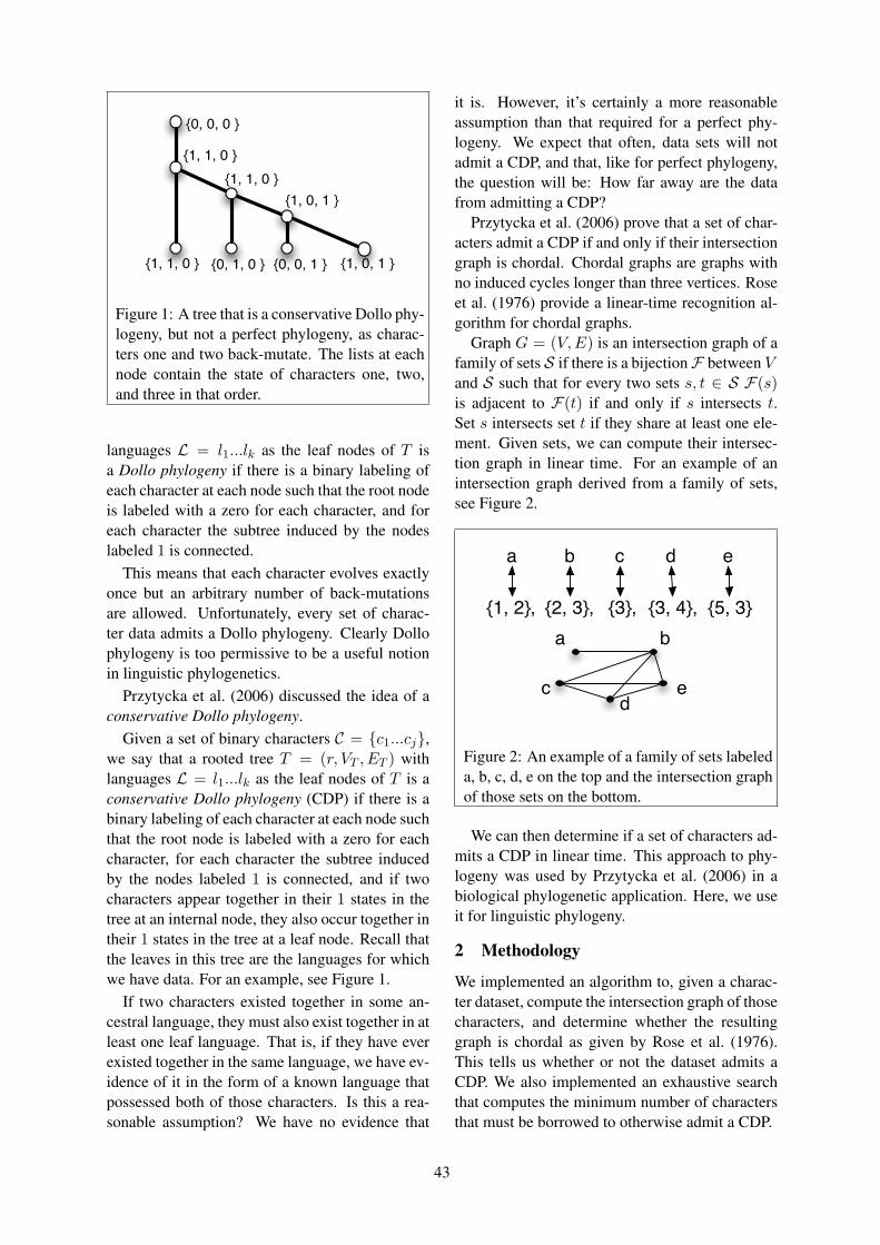
{1, 1, 0 } {0, 1, 0 } {0, 0, 1 } {1, 0, 1 }

{1, 1, 0 }{1, 1, 0 }

{0, 0, 0 }

{1, 0, 1 }

Figure 1: A tree that is a conservative Dollo phy-logeny, but not a perfect phylogeny, as charac-ters one and two back-mutate. The lists at eachnode contain the state of characters one, two,and three in that order.

languages L = l1...lk as the leaf nodes of T isa Dollo phylogeny if there is a binary labeling ofeach character at each node such that the root nodeis labeled with a zero for each character, and foreach character the subtree induced by the nodeslabeled 1 is connected.

This means that each character evolves exactlyonce but an arbitrary number of back-mutationsare allowed. Unfortunately, every set of charac-ter data admits a Dollo phylogeny. Clearly Dollophylogeny is too permissive to be a useful notionin linguistic phylogenetics.

Przytycka et al. (2006) discussed the idea of aconservative Dollo phylogeny.

Given a set of binary characters C = {c1...cj},we say that a rooted tree T = (r, VT , ET ) withlanguages L = l1...lk as the leaf nodes of T is aconservative Dollo phylogeny (CDP) if there is abinary labeling of each character at each node suchthat the root node is labeled with a zero for eachcharacter, for each character the subtree inducedby the nodes labeled 1 is connected, and if twocharacters appear together in their 1 states in thetree at an internal node, they also occur together intheir 1 states in the tree at a leaf node. Recall thatthe leaves in this tree are the languages for whichwe have data. For an example, see Figure 1.

If two characters existed together in some an-cestral language, they must also exist together in atleast one leaf language. That is, if they have everexisted together in the same language, we have ev-idence of it in the form of a known language thatpossessed both of those characters. Is this a rea-sonable assumption? We have no evidence that

it is. However, it’s certainly a more reasonableassumption than that required for a perfect phy-logeny. We expect that often, data sets will notadmit a CDP, and that, like for perfect phylogeny,the question will be: How far away are the datafrom admitting a CDP?

Przytycka et al. (2006) prove that a set of char-acters admit a CDP if and only if their intersectiongraph is chordal. Chordal graphs are graphs withno induced cycles longer than three vertices. Roseet al. (1976) provide a linear-time recognition al-gorithm for chordal graphs.

Graph G = (V,E) is an intersection graph of afamily of sets S if there is a bijectionF between Vand S such that for every two sets s, t ∈ S F(s)is adjacent to F(t) if and only if s intersects t.Set s intersects set t if they share at least one ele-ment. Given sets, we can compute their intersec-tion graph in linear time. For an example of anintersection graph derived from a family of sets,see Figure 2.

{1, 2}, {2, 3}, {3}, {3, 4}, {5, 3}

a b c d e

a b

c ed

Figure 2: An example of a family of sets labeleda, b, c, d, e on the top and the intersection graphof those sets on the bottom.

We can then determine if a set of characters ad-mits a CDP in linear time. This approach to phy-logeny was used by Przytycka et al. (2006) in abiological phylogenetic application. Here, we useit for linguistic phylogeny.

2 Methodology

We implemented an algorithm to, given a charac-ter dataset, compute the intersection graph of thosecharacters, and determine whether the resultinggraph is chordal as given by Rose et al. (1976).This tells us whether or not the dataset admits aCDP. We also implemented an exhaustive searchthat computes the minimum number of charactersthat must be borrowed to otherwise admit a CDP.

43

We ran our program on the Indo-European character dataset used by Nakhlehet al. (2005a), and available online athttp://www.cs.rice.edu/ nakhleh/CPHL/.

2.1 Language Family Grouping

Nakhleh et al. (2005a) combined established lan-guage groups into a single language during com-putation to decrease computation time. We use thesame families as they do, and do the same in twoof our experiments.

For example, we consider the Tocharian lan-guage family, consisting of Tocharian A andTocharian B to be a single language when buildingour intersection graph. This language grouping isdone as a preprocessing step to the construction ofthe intersection graph of the characters.

We expect this transformation to be particularlyuseful in the CDP setting, beyond just decreasingcomputation time. We expect it will make our datacloser to admitting a CDP in a way consistent withtrue evolutionary history.

Consider the difference between the intersec-tion graph of a set of characters with family group-ing and without. Let s and t be two characters that,are considered to intersect with family grouping,but not without. Then s and t are not present inany of the same languages, but there are two lan-guages li, lj such that li has character s but not tand language lj has character t but not s, and liand lj are in the same family L.

We use the language family definitions given byNakhleh et al. (2005a), where these language fam-ilies are identified as consistent with all characters,and it is argued that it is very unlikely there is anyborrowing between a portion of the tree inside thefamily, and a portion of the tree outside the family.

Therefore, if s and t are both present withinleaves in the language family L, and neither is bor-rowed from outside the family, then each of s, t iseither present only within language family L, oris present in at least one internal node ancestralto language family L. If s and t are only presentwithin the language family, they are not informa-tive when language family grouping is used.

However, if both s and t are present at an in-ternal node ancestral to language family L, thenthis is important information that we have derivedby applying family language grouping, and willmake the data closer to admitting a CDP in termsof number of borrowings required.

2.2 Binary DataWe made the data binary by separating states ofa given character as best indicated by notes pro-vided by Nakhleh et al. (2005a) on their coding ofthe characters. In making the data binary, we havelikely lost some constraining information. Whena language (or language family, when that group-ing was used) has a unique state at a character,we coded this as having all possible non-ancestralstates. The basis for this is that some of thesecodes indicate that there is no data for that char-acter at that language, or that if that language ac-tually does have a unique state at that character,it is uninformative, but could have evolved fromany other state. Data processing by someone morehighly trained in linguistics would either confirmthis decision or provide an alternative approach.We have tried to remain as close as possible to howthe data is used in Nakhleh et al. (2005a).

3 Experiments

We ran four experiments to investigate the use-fulness of the conservative Dollo parsimony ap-proach. We ran our implementation on:

1. All characters without language familygrouping

2. All characters with language family grouping3. Phonological and morphological characters

only without language family grouping4. Phonological and morphological characters

only with language family grouping

4 Results

We give our results in Table 4For the morphological and phonological

dataset, both grouped and ungrouped, we ex-tracted a phylogenetic tree from our program’soutput. These trees were consistent with Tree Ain (Nakhleh et al., 2005a). The fact that we man-aged to build a tree consistent with expectationswithout any input tree is very encouraging.

Recall that when we use language grouping wecombine all languages identified as being from anestablished family by Nakhleh et al. (2005a) intoa single language. For example, instead of con-sidering both Tocharian A and Tocharian B, in ourexperiments with language grouping we considera single language, Tocharian, that has all charac-teristics of Tocharian A and all characteristics ofTocharian B.

44

Table 1: The results of conservative Dollo phylogeny checking algorithm on modified versions of theIndo-European character dataset as used in (Nakhleh et al., 2005a). We ran each program for at most 1hour. Entries of ”Too slow” indicate that we did not allow the program to halt.

Dataset Admits a CDP? Minimum number of languagesthat must borrow

Answer Time Answer TimePhonological, Morphological Datawithout Language Grouping

Yes <1 s 0 <1 s

Phonological, Morphological Datawith Language Grouping

Yes <1 s 0 <1 s

All Data without Language Grouping No <1 s - Too slowAll Data with Language Grouping No <1 s 2 < 1 s

In our experiments without language grouping,we do not combine languages in this way, and in-stead consider all 24 languages separately.

5 Discussion

When is the CDP approach useful for linguisticphylogenetics?

Because a CDP allows back-mutation, it islikely most useful for datasets that exhibit a lot ofback mutation, and not a lot of borrowing. Phono-logical and morphological characters are morelikely to fit this requirement than lexical data. Thisis reflected in our positive results on the phonolog-ical and morphological characters alone.

In contrast, when we included the lexical data,the dataset did not admit a conservative Dollo par-simony, whether or not we used language familygrouping. We expect this is due to borrowing oflexical characters.

The full dataset with language family group-ing was much closer to admitting a conserva-tive Dollo parsimony than the full dataset with-out language family grouping. As explained in ourMethodology section, this was expected and rein-forces our position that language family groupingis extremely useful when computing conservativeDollo phylogenies.

Our experiments ran in either negligible time,or were not allowed to halt. The speed of the fastexperiments suggests that computing conservativeDollo phylogenies might be useful in construct-ing a tree when no tree is known, and the amountof character data causes computing other types ofphylogenies to be intractable.

6 Future Work

We are currently pursuing several extensions tothis work.

First, we are developing an improved heuristicsearch for the minimum number of edges that needto be removed from or added to a graph to makethe resulting graph chordal. This will enable us touse the Dollo phylogeny approach outlined hereon character data sets that require more borrowingto fully explain them.

Using this improved search, we will run experi-ments on other sets of character data.

Nakhleh et al. (2005a) started with several pro-posed trees in their work on perfect phylogeneticnetworks. We plan to implement a version of ourCDP approach that takes as input a proposed tree.This version will calculate the minimum numberof edges that must be added to create a Dollophylogeny network, as analogous to Nakhleh etal.’s perfect phylogenetic network. This minimumnumber of edges would be useful as a lower boundfor the required number of edges one must add toproduce a perfect phylogeny network.

7 Conclusion

We have presented an alternative phylogeny thatmay be of use in linguistic phylogenetics, par-ticularly on phonological or morphological data.We have proposed a number of future extensionsbased on our experiments that we hope will im-prove the performance of this approach.

Acknowledgments

The author would like to acknowledge the helpfulinput of reviewers, as well as Dr. Gzegorz Kon-drak and Dr. Lorna Stewart.

45

ReferencesWilliam Day, David Johnson, and David Sankoff.

1986. The computational complexity of inferringrooted phylogenies by parsimony. MathematicalBiosciences, 81:33–42.

Joseph Felsenstein. 2004. Inferring Phyloge-nies. Number 1. Sinauer Associates, Massachusetts,USA.

Luay Nakhleh, Don Ringe, and Tandy Warnow. 2005a.Perfect phylogenetic networks: A new methodologyfor reconstructing the evolutionary history of natu-ral languages. Language (Journal of the LinguisticSociety of America), 81(2):382–420.

Luay Nakhleh, Tandy Warnow, Don Ringe, andSteven N. Evans. 2005b. A comparison of phyloge-netic reconstruction methods on an ie dataset. TheTransactions of the Philological Society, 3(2):171 –192.

Teresa Przytycka, George Davis, Nan Song, and Dan-nie Durand. 2006. Graph theoretical insights intoevolution of multidomain proteins. Journal of com-putational biology : a journal of computationalmolecular cell biology, 13(2):351–363.

Donald J. Rose, R. Endre Tarjan, and George S. Leuker.1976. Algorithmic aspects of vertex elimination ongraphs. SIAM Journal of Computing, 5(2):266–283.

46

Proceedings of the 2010 Workshop on Graph-based Methods for Natural Language Processing, ACL 2010, page 47,Uppsala, Sweden, 16 July 2010. c©2010 Association for Computational Linguistics

Spectral Approaches to Learning in the Graph Domain

Edwin HancockDepartment of Computer Science

University of YorkYork YO10 5DD, UK

erh@cs.york.ac.uk

Abstract

The talk will commence by discussing some of the problems that arise when machine learning isapplied to graph structures. A taxonomy of different methods organised around a) clustering b)characterisation and c) constructing generative models in the graph domain will be introduced.With this taxonomy in hand, Dr. Hancock will then describe a number of graph-spectral al-gorithms that can be applied to solve the many different problems inherent to graphs, drawingexamples from computer vision research.

47

Proceedings of the 2010 Workshop on Graph-based Methods for Natural Language Processing, ACL 2010, pages 48–54,Uppsala, Sweden, 16 July 2010. c©2010 Association for Computational Linguistics

Cross-lingual comparison between distributionally determinedword similarity networks

Olof GornerupSwedish Institute of Computer Science

(SICS)164 29 Kista, Swedenolofg@sics.se

Jussi KarlgrenSwedish Institute of Computer Science

(SICS)164 29 Kista, Swedenjussi@sics.se

Abstract

As an initial effort to identify universaland language-specific factors that influ-ence the behavior of distributional models,we have formulated a distributionally de-termined word similarity network model,implemented it for eleven different lan-guages, and compared the resulting net-works. In the model, vertices constitutewords and two words are linked if they oc-cur in similar contexts. The model is foundto capture clear isomorphisms across lan-guages in terms of syntactic and semanticclasses, as well as functional categories ofabstract discourse markers. Language spe-cific morphology is found to be a dominat-ing factor for the accuracy of the model.

1 Introduction

This work takes as its point of departure the factthat most studies of the distributional character ofterms in language are language specific. A modelor technique—either geometric (Deerwester et al.,1990; Finch and Chater, 1992; Lund and Burgess,1996; Letsche and Berry, 1997; Kanerva et al.,2000) or graph based (i Cancho and Sole, 2001;Widdows and Dorow, 2002; Biemann, 2006)—that works quite well for one language may not besuitable for other languages. A general questionof interest is then: What strengths and weaknessesof distributional models are universal and what arelanguage specific?

In this paper we approach this question by for-mulating a distributionally based network model,apply the model on eleven different languages, andthen compare the resulting networks. We com-pare the networks both in terms of global statisti-cal properties and local structures of word-to-wordrelations of linguistic relevance. More specif-ically, the generated networks constitute words

(vertices) that are connected with edges if theyare observed to occur in similar contexts. Thenetworks are derived from the Europarl corpus(Koehn, 2005)—the annotated proceedings of theEuropean parliament during 1996-2006. This isa parallel corpus that covers Danish, Dutch, En-glish, Finnish, French, German, Greek, Italian,Portuguese, Spanish and Swedish.

The objective of this paper is not to provide aextensive comparison of how distributional net-work models perform in specific applications forspecific languages, for instance in terms of bench-mark performance, but rather to, firstly, demon-strate the expressive strength of distributionallybased network models and, secondly, to highlightfundamental similarities and differences betweenlanguages that these models are capable of captur-ing (and fail in capturing).

2 Methods

We consider a base case where a context is definedas the preceding and subsequent words of a focusword. Word order matters and so a context formsa word pair. Consider for instance the followingsentence1:

Ladies and gentlemen, once again, wesee it is essential for Members to bringtheir voting cards along on a Monday.

Here the focus wordessentialoccurs in the con-text is ∗ for, the wordbring in the contextto ∗their etcetera (the asterisk∗ denotes an interme-diate focus word). Since a context occurs with aword with a certain probability, each wordwi isassociated with a probability distribution of con-texts:

Pi = {Pr[wpwiws|wi]}wp,ws∈W , (1)

1Quoting Nicole Fontaine, president of the European Par-liament 1999-2001, from the first session of year 2000.

48

where W denotes the set of all words andPr[wpwiws|wi] is the conditional probability thatcontextwp ∗ws occurrs, given that the focus wordis wi. In practice, we estimatePi by countingthe occurring contexts ofwi and then normalizingthe counts. Context counts, in turn, were derivedfrom trigram counts. No pre-processing, such asstemming, was performed prior to collecting thetrigrams.

2.1 Similarity measure

If two words have similar context distributions,they are assumed to have a similar function inthe language. For instance, it is reasonable to as-sume that the word “salt” to a higher degree occursin similar contexts as “pepper” compared to, say,“friendly”. One could imagine that a narrow 1+1neighborhood only captures fundamental syntacticagreement between words, which has also been ar-gued in the literature (Sahlgren, 2006). However,as we will see below, the intermediate two-wordcontext also captures richer word relationships.

We measure the degree of similarity by com-paring the respective context distributions. Thiscan be done in a number of ways. For example,as the Euclidian distance (also known as L2 diver-gence), the Harmonic mean, Spearman’s rank cor-relation coefficient and the Jensen-Shannon diver-gence (information radius). Here we quantify thedifference between two wordswi andwj , denoteddij , by the variational distance (or L1 divergence)between their corresponding context distributionsPi andPj :

dij =∑

c∈C|Pi(X = c)− Pj(X = c)|, (2)

whereX is a stochastic variable drawn fromC,which is the set of contexts that eitherwi or wjoccur in. 0 ≤ dij ≤ 2, where dij = 0 ifthe two distributions are identical anddij = 2if the words do not share any contexts at all. Itis not obvious that the variational distance is thebest choice of measure. However, we chose toemploy it since it is a well-established and well-understood statistical measure; since it is straight-forward and fast to calculate; and since it appearsto be robust. To compare, we have also testedto employ the Jensen-Shannon divergence (a sym-metrized and smoothed version of Kullback infor-mation) and acquire very similar results as thosepresented here. In fact, this is expected since the

two measures are found to be approximately lin-early related in this context. However, for the twofirst reasons listed above, the variational distanceis our divergence measure of choice in this study.

2.2 Network representation

A set of words and their similarity relations arenaturally interpreted as a weighted and undirectednetwork. The vertices then constitute words andtwo vertices are linked by an edge if their corre-sponding wordswi andwj have overlapping con-text sets. The strength of the links vary depend-ing on the respective degrees of word similarities.Here the edge between two wordswi andwj ’sis weighted withwij = 2 − dij (note again thatmaxij dij = 2) since a large word difference im-plies a weak link and vice versa.

In our experiment we consider the 3000 mostcommon words, excluding the 19 first ones, ineach language. To keep the data more manage-able during analysis we employ various thresh-olds. Firstly, we only consider context words thatoccur five times or more. As formed by the re-maining context words, we then only consider tri-grams that occur three times or more. This allowsus to cut away a large chunk of the data. We havetested to vary these thresholds and the resultingnetworks are found to have very similar statisti-cal properties, even though the networks differ bya large number of very weak edges.

3 Results

3.1 Degree distributions

The degreegi of a vertexi is defined as the sumof weights of the edges of the vertex:gi =

∑wij .

The degree distribution of a network may providevaluable statistical information about the networksstructure. For the word networks, Figure 1, the de-gree distributions are all found to be highly right-skewed and have longer tails than expected fromrandom graphs (Erdos and Renyi, 1959). Thischaracteristics is often observed in complex net-works, which typically also are scale-free (New-man, 2003). Interestingly, the word similarity net-works are not scale-free as their degree distribu-tions do no obey power-laws:Pr(g) ∼ g−α forsome exponentα. Instead, the degree distributionsof each word network appears to lay somewherebetween a power-law distribution and an exponen-tial distribution (Pr(g) ∼ e−g/κ). However, dueto quite noisy statistics it is difficult to reliably

49

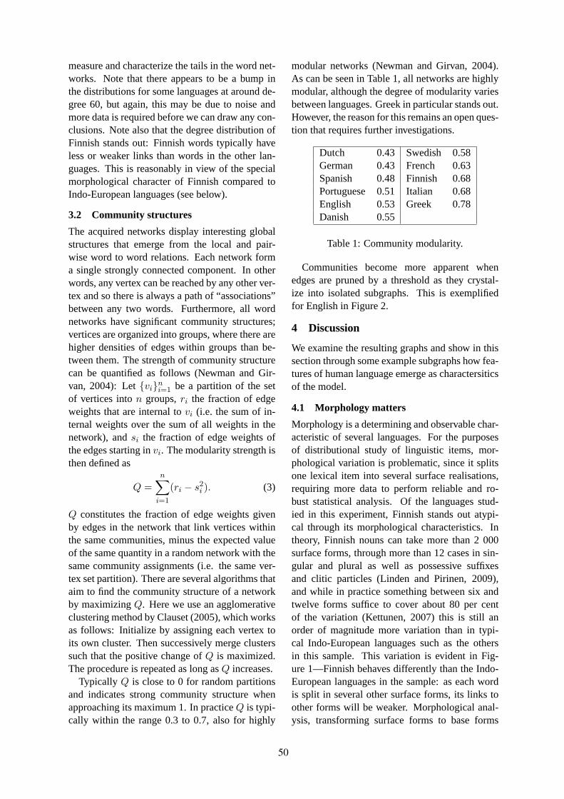
measure and characterize the tails in the word net-works. Note that there appears to be a bump inthe distributions for some languages at around de-gree 60, but again, this may be due to noise andmore data is required before we can draw any con-clusions. Note also that the degree distribution ofFinnish stands out: Finnish words typically haveless or weaker links than words in the other lan-guages. This is reasonably in view of the specialmorphological character of Finnish compared toIndo-European languages (see below).

3.2 Community structures

The acquired networks display interesting globalstructures that emerge from the local and pair-wise word to word relations. Each network forma single strongly connected component. In otherwords, any vertex can be reached by any other ver-tex and so there is always a path of “associations”between any two words. Furthermore, all wordnetworks have significant community structures;vertices are organized into groups, where there arehigher densities of edges within groups than be-tween them. The strength of community structurecan be quantified as follows (Newman and Gir-van, 2004): Let{vi}ni=1 be a partition of the setof vertices inton groups,ri the fraction of edgeweights that are internal tovi (i.e. the sum of in-ternal weights over the sum of all weights in thenetwork), andsi the fraction of edge weights ofthe edges starting invi. The modularity strength isthen defined as

Q =n∑

i=1

(ri − s2i ). (3)

Q constitutes the fraction of edge weights givenby edges in the network that link vertices withinthe same communities, minus the expected valueof the same quantity in a random network with thesame community assignments (i.e. the same ver-tex set partition). There are several algorithms thataim to find the community structure of a networkby maximizingQ. Here we use an agglomerativeclustering method by Clauset (2005), which worksas follows: Initialize by assigning each vertex toits own cluster. Then successively merge clusterssuch that the positive change ofQ is maximized.The procedure is repeated as long asQ increases.

Typically Q is close to 0 for random partitionsand indicates strong community structure whenapproaching its maximum 1. In practiceQ is typi-cally within the range 0.3 to 0.7, also for highly

modular networks (Newman and Girvan, 2004).As can be seen in Table 1, all networks are highlymodular, although the degree of modularity variesbetween languages. Greek in particular stands out.However, the reason for this remains an open ques-tion that requires further investigations.

Dutch 0.43 Swedish 0.58German 0.43 French 0.63Spanish 0.48 Finnish 0.68Portuguese 0.51 Italian 0.68English 0.53 Greek 0.78Danish 0.55

Table 1: Community modularity.

Communities become more apparent whenedges are pruned by a threshold as they crystal-ize into isolated subgraphs. This is exemplifiedfor English in Figure 2.

4 Discussion

We examine the resulting graphs and show in thissection through some example subgraphs how fea-tures of human language emerge as charactersiticsof the model.

4.1 Morphology matters

Morphology is a determining and observable char-acteristic of several languages. For the purposesof distributional study of linguistic items, mor-phological variation is problematic, since it splitsone lexical item into several surface realisations,requiring more data to perform reliable and ro-bust statistical analysis. Of the languages stud-ied in this experiment, Finnish stands out atypi-cal through its morphological characteristics. Intheory, Finnish nouns can take more than 2 000surface forms, through more than 12 cases in sin-gular and plural as well as possessive suffixesand clitic particles (Linden and Pirinen, 2009),and while in practice something between six andtwelve forms suffice to cover about 80 per centof the variation (Kettunen, 2007) this is still anorder of magnitude more variation than in typi-cal Indo-European languages such as the othersin this sample. This variation is evident in Fig-ure 1—Finnish behaves differently than the Indo-European languages in the sample: as each wordis split in several other surface forms, its links toother forms will be weaker. Morphological anal-ysis, transforming surface forms to base forms

50

0

200

400

600

800

1000

1200

1400

1600

1800

0 50 100 150 200 250 300 350

degr

ee c

ount

degree

DanishGerman

GreekEnglishSpanishFinnishFrenchItalianDutch

PortugueseSwedish

Figure 1: Degree histograms of word similarity networks.

# %

#%

l' activité

l' adhésionl' adoption

l' amélioration

l' application

l' augmentation

l' égalitél' élaboration

l' établissement

l' évaluationl' examen

l' exécution

l' existencel' harmonisation

l' histoire

l' interdiction

l' intervention

l' introduction

l' octroi l' ouverture

l' utilisation

l adhésionl adoption l application

l égalité

l élargissement

l ensemble

l utilisation

Figure 3: French definite nouns clustered.

would strengthen those links.

In practice, the data sparsity caused by mor-phological variation causes semantically homoge-nous classes to be split. Even for languages suchas English and French, with very little data varia-tion we find examples where morphological varia-tion causes divergence as seen in Figure 3, whereFrench nouns in definite form are clustered. It isnot surprising that certain nouns in definite formassume similar roles in text, but the neatness ofthe graph is a striking exposition of this fact.

These problems could have been avoided withbetter preprocessing—simple such processing inthe case of English and French, and considerablymore complex but feasible in the case of Finnish—but are retained in the present example as proxiesfor the difficulties typical of processing unknownlanguages. Our methodology is robust even inface of shoddy preprocessing and no knowledgeof the morphological basis of the target language.In general, as a typological fact, it is reasonable to

assume that morphological variation is offset forthe language user in a greater freedom in choice ofword order. This would seem to cause a great dealof problems for an approach such as the presentone, since it relies on the sequential organisationof symbols in the signal. However, it is observ-able that languages with free word order have pre-ferred unmarked arrangements for their sentencestructure, and thus we find stable relationships inthe data even for Finnish, although weaker than forthe other languages examined.

4.2 Syntactic classes

Previous studies have shown that a narrow con-text window of one neighour to the left and oneneighbour to the right such as the one used inthe present experiments retrieves syntactic rela-tionships (Sahlgren, 2006). We find several suchexamples in the graphs. In Figure 2 we can seesubgraphs with past participles, auxiliary verbs,progressive verbs, person names.

4.3 Semantic classes

Some of the subgraphs we find are models of clearsemantic family resemblance as shown in Fig-ure 4. This provides us with a good argument forblurring the artificial distinction between syntaxand semantics. Word classes are defined by theirmeaning and usage alike; thea priori distinctionbetween classification by function such as auxil-iary verbs given above and classification by mean-ing such months and places given here is not fruit-ful. We expect to be able to provide much more in-

51

adapt

addition

address

afghanistanalbania

algeria

amend

amsterdam

asia

assess

auditors

austria barcelona

belarus

belgium

berlin

bosnia

britain

brussels

bulgaria

burma

chechnya

china

clarify

clarity

coherence

competitiveness

condemn

coordinate

copenhagencorruption

croatiacuba

culture

cyprus

define

denmark

discuss

dublin

efficiency

eliminate

employers

emu

enhance

europol

examine

expression

finland

flexibility

france

fraud

fulfil

genevagermany

globalisation

gmos

greece

harmonisation

harmonization

helsinki

implement

improve

incorporate

india

indonesia

innovation

inquiry

iraniraq

ireland

israel

issue

italy

japan

kind

kosovo

liberalisation

londonluxembourg

macedonia

maintain

matter

men

ministers

monitor

afternoon

evening morning

morocco

movement

nato

nice

olaf

openness

oppose

order

origin

overcome

palestine

articles

paragraphparagraphs

parliament'

people'

poland

politics

portugal

poverty

preserve

presidents

abolition

absence

adoption

aim

appointment

background

chairman

completion

concept

continuationcreation

definition

establishment

event

face

grounds

inclusionintroduction

leader

lightmiddle

occasion

possibilitypromotion

prospectpurpose

purposes

pursue

racism

ratify

regulate

reinforce

reject

relation

religion

remove

replace

resolve

retain

romania

russia

safeguard

science

considering

debating

discussing

examining aims

fails

refers

seeks

april

december

february

january

july

june

march

november

october

september

serbia

slovakia

covers

includes

involvesreflects barroso

prodi

santer

solana

solve

sort

spain

sport

strasbourg

strengthen

addressed

applied

completed

condemned

conducted

created

debated

discussed

encouraged

established

examined

financed

funded

guaranteedimplemented

improved

introduced

justified

maintained

monitored

promoted

protectedpursued

regulated resolved

respected

solved

strengthened

confirmed

emphasised

highlighted noted

stressed

subject

subsidiarity

afraid

delighted

glad

happy

pleased

sorry

sure

sweden

austrian belgian

danish

dutch

finnish

french

german

greek

irish

italianportuguese

spanish swedish

tackle

achievingaddressing applying

changing

defending

defining

guaranteeing

implementingmaintaining

protecting

safeguardingsupporting

tackling

tampere

terrorism

believe

feel

hopethink

foremost

hence

secondly

thirdly

torture

tourism

transparency

treat

turkey

five

four

seven

ten

three

two

type

ukraine

acknowledgeemphasise

emphasize

highlight

raise

realise

recognise

recognize

reiterate

remember

stress

underline

unemployment

apparentevidentobvious

regrettable

true

unfortunate

union'

appearbelongfailrefuse seem

ask inviteremind urge

americans

balkans

bureau

cap

citizen

courts

ecb

euro

factsgreens

ground

igc

internet

netherlands

ombudsmanpalestinians

railways roadss

treatiesuk

usa

vienna

crucial

essential

unacceptable

vital

ableentitled

going

prepared supposed

willing

intend

want wish

continues intends

wants

wishes

withdraw

childrenconsumers

employeesfarmersfishermen

forests

immigrants

individuals

journalists

minorities

ngos

producers

refugeessmesstudentswomen

workers

must

should

will

would

days

months

weeks

years

zimbabwe

Figure 2: English. Network involving edges with weightsw ≥ 0.85. For sake of clarity, only subgraphswith three or more words are shown. Note that the threshold 0.85 is used only for the visualization. Thefull network consists of the 3000 most common words in English, excluding the 19 most common ones.

52

avril

décembre

févrierjanvier

juillet

juin

mai

mars

novembre

octobre

septembre

april

december

februari

januari

juli juni

maj

mars

november

oktoberseptember

enhance

improve

preserve

reinforcesafeguard strengthen

corruption fraud

poverty

racism

terrorism

torture

Figure 4: Examples of semantically homogenousclasses in English, French and Swedish.

formed classification schemes than the traditional“parts of speech” if we define classes by their dis-tributional qualities rather than by the “content”they “represent”, schemes which will cut acrossthe function-topic distinction.

4.4 Abstract discourse markers are afunctional category

Further, several subgraphs have clear collectionsof discourse markers of various types where theterms are markers of informational organisation inthe text, as exemplified in Figure 5.

5 Conclusions

This preliminary experiment supports future stud-ies to build knowledge structures across lan-guages, using distributional isomorphism betweenlinguistic material in translated or even compara-ble corpora, on several levels of abstraction, fromfunction words, to semantic classes, to discoursemarkers. The isomorphism across the languagesis clear and incontrovertible; this will allow us tocontinue experiments using collections of multi-lingual materials, even for languages with rela-tively little technological support. Previous stud-ies show that knowledge structures of this typethat are created in one language show consider-able isomorphism to knowledge structures createdin another language if the corpora are comparable(Holmlund et al., 2005). Holmlund et al show howtranslation equivalences can be established using

epäilemättä

kuitenkin

luonnollisesti

selvästikin

siis

tietenkin

tietysti

todellakin

toki

varmasti

förmodligen

förvisso

givetvis

säkerligen

sannerligen

självfallet

uppenbarligen

visserligen

Figure 5: Examples of discourse functional classesin Swedish and Finnish. The terms in the two sub-graphs are discourse markers and correspond toEnglish “certainly”, “possibly”, “evidently”, “nat-urally”, “absolutely”, “hence” and similar terms.

two semantic networks automatically created intwo languages by providing a relatively limited setof equivalence relations in a translation lexicon.This study supports those findings.

The results presented here display the potentialof distributionally derived network representationsof word similarities. Although geometric (vectorbased) and probabilistic models have proven vi-able in various applications, they are limited bythe fact that word or term relations are constrainedby the geometric (often Euclidian) space in whichthey live. Network representations are richer inthe sense that they are not bound by the same con-straints. For instance, a polyseme word (“may” forexample) can have strong links to two other words(“might” and ”September” for example), wherethe two other words are completely unrelated. Inan Euclidean space this relation is not possible dueto the triangle inequality. It is possible to em-bed a network in a geometric space, but this re-quires a very high dimensionality which makes therepresentation both cumbersome and inefficient interms of computation and memory. This has beenaddressed by coarse graining or dimension reduc-tion, for example by means of singular value de-

53

composition (Deerwester et al., 1990; Letsche andBerry, 1997; Kanerva et al., 2000), which resultsin information loss. This can be problematic, inparticular since distributional models often facedata sparsity due to the curse of dimensionality.In a network representation, such dimension re-duction is not necessary and so potentially impor-tant information about word or term relations isretained.

The experiments presented here also show thepotential of moving from a purely probabilisticmodel of term occurrence, or a bare distributionalmodel such as those typically presented using ageometric metaphor, in that it affords the possibil-ity of abstract categories inferred from the primarydistributional data. This will give the possibilityof further utilising the results in studies, e.g. forlearning syntactic or functional categories in morecomplex constructional models of linguistic form.Automatically establishing lexically and function-ally coherent classes in this manner will have bear-ing on future project goals of automatically learn-ing syntactic and semantic roles of words in lan-guage. This target is today typically pursued rely-ing on traditional lexical categories which are notnecessarily the most salient ones in view of actualdistributional characteristics of words.Acknowledgments: OG was supported by Johanand Jacob Soderberg’s Foundation. JK was sup-ported by the Swedish Research Council.

References

Chris. Biemann. 2006. Chinese whispers - an efficientgraph clustering algorithm and its application to nat-ural language processing problems. InProceedingsof the HLT-NAACL-06 Workshop on Textgraphs-06,New York, USA.

Aaron Clauset. 2005. Finding local community struc-ture in networks.Physical Review E, 72:026132.

Scott Deerwester, Susan T. Dumais, George W. Furnas,Thomas K. Landauer, and Richard Harshman. 1990.Indexing by latent semantic analysis.Journal of theAmerican Society for Information Science, 41:391–407.

Pal Erdos and Alfred Renyi. 1959. On random graphs.Publications Mathematicae, 6:290.

Steven Finch and Nick Chater. 1992. Bootstrap-ping syntactic categories. InProceedings of theFourteenth Annual Conference of the Cognitive Sci-ence Society, pages 820–825, Bloomington, IN.Lawrence Erlbaum.

Jon Holmlund, Magnus Sahlgren, and Jussi Karlgren.2005. Creating bilingual lexica using referencewordlists for alignment of monolingual semanticvector spaces. InProceedings of 15th Nordic Con-ference of Computational Linguistics.

Ramon Ferrer i Cancho and Ricard V. Sole. 2001. Thesmall world of human language.Proceedings of theRoyal Society of London. Series B, Biological Sci-ences, 268:2261–2266.

Pentti Kanerva, Jan Kristoferson, and Anders Holst.2000. Random indexing of text samples for latentsemantic analysis. InProceedings of the 22nd An-nual Conference of the Cognitive Science Society,pages 103–6.

Kimmo Kettunen. 2007. Management of keywordvariation with frequency based generation of wordforms in ir. InProceedings of SIGIR 2007.

Philipp Koehn. 2005. Europarl: A parallel corpus forstatistical machine translation. InMT Summit.

Todd Letsche and Michael Berry. 1997. Large-scaleinformation retrieval with latent semantic indexing.Information Sciences, 100(1-4):105–137.

Krister Linden and Tommi Pirinen. 2009. Weightingfinite-state morphological analyzers using hfst tools.In Proceedings of the Finite-State Methods and Nat-ural Language Processing. Pretoria, South Africa.

Kevin Lund and Curt Burgess. 1996. Producinghigh-dimensional semantic spaces from lexical co-occurrence. Behavior Research Methods, Instru-ments, and Computers, 28(2):203–208.

Mark Newman and Michelle Girvan. 2004. Find-ing and evaluating community structure in networks.Physical Review E, 69(2).

Mark E. J. Newman. 2003. The structure and functionof complex networks. SIAM Review, 45(2):167–256.

Magnus Sahlgren. 2006.The Word-Space Model: Us-ing distributional analysis to represent syntagmaticand paradigmatic relations between words in high-dimensional vector spaces. PhD Dissertation, De-partment of Linguistics, Stockholm University.

Dominic Widdows and Beate Dorow. 2002. A graphmodel for unsupervised lexical acquisition. InIn19th International Conference on ComputationalLinguistics, pages 1093–1099.

54

Proceedings of the 2010 Workshop on Graph-based Methods for Natural Language Processing, ACL 2010, pages 55–59,Uppsala, Sweden, 16 July 2010. c©2010 Association for Computational Linguistics

Co-occurrence Cluster Features for Lexical Substitutions in Context

Chris BiemannPowerset (a Microsoft company)

475 Brannan St Ste. 330San Francisco, CA 94107, USAcbiemann@microsoft.com

AbstractThis paper examines the influence of fea-tures based on clusters of co-occurrencesfor supervised Word Sense Disambigua-tion and Lexical Substitution. Co-occurrence cluster features are derivedfrom clustering the local neighborhood ofa target word in a co-occurrence graphbased on a corpus in a completely un-supervised fashion. Clusters can be as-signed in context and are used as featuresin a supervised WSD system. Experi-ments fitting a strong baseline system withthese additional features are conducted ontwo datasets, showing improvements. Co-occurrence features are a simple way tomimic Topic Signatures (Martınez et al.,2008) without needing to construct re-sources manually. Further, a system is de-scribed that produces lexical substitutionsin context with very high precision.

1 Introduction

Word Sense Disambiguation (WSD, see (Agirreand Edmonds, 2006) for an extensive overview)is commonly seen as an enabling technology forapplications like semantic parsing, semantic rolelabeling and semantic retrieval. Throughout re-cent years, the Senseval and Semeval competitionshave shown that a) WordNet as-is is not an ade-quate semantic resource for reaching high preci-sion and b) supervised WSD approaches outper-form unsupervised (i.e. not using sense-annotatedexamples) approaches. Due to the manual effortinvolved in creating more adequate word sense in-ventories and sense-annotated training data, WSDhas yet to see its prime-time in real world applica-tions.

Since WordNet’s sense distinctions are often toofine-grained for allowing reliable distinctions bymachines and humans, the OntoNotes project(Hovy et al., 2006) conflated similar WordNetsenses until 90% inter-annotator agreement onsense-labelling was reached. The SemEval 2007lexical sample task employs this ”coarse-grained”inventory, which allows for higher system perfor-mance.To alleviate the bottleneck of sense-labelled sen-tences, (Biemann and Nygaard, 2010) presentan approach for acquiring a sense inventoryalong with sense-annotated example usages usingcrowdsourcing, which makes the acquisition pro-cess cheaper and potentially quicker.Trying to do away with manual resources entirely,the field of Word Sense Induction aims at induc-ing the inventory from text corpora by clusteringoccurrences or senses according to distributionalsimilarity, e.g. (Veronis, 2004). While such unsu-pervised and knowledge-free systems are capableof discriminating well between different usages, itis not trivial to link their distinctions to existing se-mantic resources, which is often necessary in ap-plications.Topic Signatures (Martınez et al., 2008) is an at-tempt to account for differences in relevant topicsper target word. Here, a large number of contextsfor a given sense inventory are collected automat-ically using relations from a semantic resource,sense by sense. The most discriminating contentwords per sense are used to identify a sense inan unseen context. This approach is amongst themost successful methods in the field. It requires,however, a semantic resource of sufficient detailand size and a sense-labeled corpus to estimatepriors from the sense distribution. Here, a sim-ilar approach is described that uses an unlabeled

55

corpus alone for unsupervised topic signature ac-quisition using graph clustering, not relying on theexistence of a WordNet. Unlike in previous eval-uations like (Agirre et al., 2006), parameters forword sense induction are not optimized globally,but instead several parameter settings are offeredas features to a Machine Learning setup.Experimental results are provided for two datasets:the Semeval-2007 lexical sample task (Pradhan etal., 2007) and the Turk bootstrap Word Sense In-ventory (TWSI1, (Biemann and Nygaard, 2010) ).

2 Cluster Co-occurrence Features

2.1 Graph Preperation and Parameterization

Similar to the approach in (Widdows and Dorow,2002), a word graph around each target wordis constructed. In this work, sentence-basedco-occurrence statistics from a large corpus areused as a basis to to construct several wordgraphs for different parameterizations. Significantco-occurrences between all content words (nouns,verbs, adjectives as identified by POS tagging) arecomputed from a large corpus using the tinyCC2

tool. The full word graph for a target word is de-fined as all words significantly co-occurring withthe target as nodes, with edge weights set to thelog-likelihood significance of the co-occurrencebetween the words corresponding to nodes. Edgesbetween words that co-occur only once or withsignificance smaller than 6.63 (1% confidencelevel) are omitted.Aiming at different granularities of usage clusters,the graph is parameterized by a size parametert and a density parameter n: Only the mostsignificant t co-occurrences of the target enter thegraph as nodes, and an edge between nodes isdrawn only if one of the corresponding words iscontained in the most significant n co-occurrencesof the other.

2.2 Graph Clustering Parameterization

As described in (Biemann, 2006), the neighbor-hood graph is clustered with Chinese Whispers.This efficient graph clustering algorithm finds thenumbers of clusters automatically and returns apartition of the nodes. It is initialized by assigningdifferent classes to all nodes in the graph. Then,

1full dataset available for download athttp://aclweb.org/aclwiki/index.php?title=Image:TWSI397.zip

2http://beam.to/biem/software/TinyCC2.html

a number of local update steps are performed, inwhich a node inherits the predominant class in itsneighborhood. At this, classes of adjacent nodesare weighted by edge weight and downweightedby the degree (number of adjacent nodes) of theneighboring node. This results in hard clusters ofwords per target, which represent different targetusages.Downweighting nodes by degree is done accord-ing to the following intuition: nodes with highdegrees are probably very universally used wordsand should be less influential for clustering. Threeways of node weighting are used: (a) dividing theinfluence of a node in the update step by the degreeof the node, (b) dividing by the natural logarithmof the degree + 1 and (c) not doing node weight-ing. The more aggressive the downweighting, thehigher granularity is expected for the clustering.It is emphasized that no tuning techniques are ap-plied to arrive at the ’best’ clustering. Rather, sev-eral clusterings of different granularities as fea-tures are made available to a supervised system.Note that this is different from (Agirre et al.,2006), where a single global clustering was useddirectly in a greedy mapping to senses.

2.3 Feature Assignment in ContextFor a given occurrence of a target word, theoverlap in words between the textual contextand all clusters from the neighborhood graph ismeasured. The cluster ID of the cluster with thehighest overlap is assigned as a feature. This canbe viewed as a word sense induction system in itsown right.At this, several clusterings from different param-eterizations are used to form distinct features,which enables the machine learning algorithm topick the most suitable cluster features per targetword when building the classification model.

2.4 Corpora for Cluster FeaturesWhen incorporating features that are induced us-ing large unlabeled corpora, it is important to en-sure that the corpus for feature induction and theword sense labeled corpus are from the same do-main, ideally from the same source.Since TWSI has been created from Wikipedia, anEnglish Wikipedia dump from January 2008 isused for feature induction, comprising a total of 60million sentences. The source for the lexical sam-ple task is the Wall Street Journal, and since the

56

76,400 sentences from the WSJ Penn Treebank arerather small for co-occurrence analysis, a 20 Mil-lion sentence New York Times corpus was usedinstead.For each corpus, a total of 45 different clus-terings were prepared for all combinations oft={50,100,150,200,250}, n={50,100,200} andnode degree weighting options (a), (b) and (c).

3 Experimental Setup

3.1 Machine Learning Setup

The classification algorithm used throughout thiswork is the AODE (Webb et al., 2005) classifieras provided by the WEKA Machine Learningsoftware (Hall et al., 2009). This algorithm issimilar to a Naıve Bayes classifier. As opposedto the latter, AODE does not assume mutualindependence of features but models correlationsbetween them explicitly, which is highly desirablehere since both baseline and co-occurrence clusterfeatures are expected to be highly correlated.Further, AODE handles nominal features, so it isdirectly possible to use lexical features and clusterIDs in the classifier. AODE showed superiorperformance to other classifiers handling nominalfeatures in preliminary experiments.

3.2 Baseline System

The baseline system relies on 15 lexical and POS-based nominal features: word forms left and rightfrom target, POS sequences left and right bigramaround target, POS tags of left and right word fromtarget, and POS tag of target, two left and two rightnouns from target, left and right verbs from targetand left and right adjectives from target.

3.3 Feature Selection

To determine the most useful cluster co-occurrence features, they were added to thebaseline features one at the time, measuring thecontribution using 10-fold cross validation onthe training set. Then, the best k single clusterfeatures for k={2,3,5,10} were added togetherto account for a range of different granularities.The best performing system on the lexical sampletraining data resulted in a 10-fold accuracy of88.5% (baseline: 87.1%) for k=3. On the 204ambiguous words (595 total senses with 46sentences per sense on average) of the TWSIonly, the best system was found at k=5 with a

System F1NUS-ML 88.7% ± 1.2top3 cluster, optimal F1 88.0% ± 1.2top3 cluster, max recall 87.8% ± 1.2baseline, optimal F1 87.5% ± 1.2baseline, max recall 87.3% ± 1.2UBC-ALM 86.9% ± 1.2

Table 1: Cluster co-occurrence features and base-line in comparison to the best two systems in theSemEval 2007 Task 17 Lexical Sample evaluation(Pradhan et al., 2007). Error margins provided bythe task organizers.

10-fold accuracy of 83.0% (baseline: 80.7%,MFS: 71.5%). Across the board, all singleco-occurrence features improve over the baseline,most of them significantly.

4 Results

4.1 SemEval 2007 lexical sample task

The system in the configuration determined abovewas trained on the full training set and applied itto the test data provided bt the task organizers.Since the AODE classifier reports a confidencescore (corresponding to the class probability forthe winning class at classification time), it is possi-ble to investigate a tradeoff between precision andrecall to optimize the F1-value3 used for scoringin the lexical sample task.

It is surprising that the baseline system outper-forms the second-best system in the 2007 evalua-tion, see Table 1. This might be attributed to theAODE classifier used, but also hints at the powerof nominal lexical features in general.The co-occurrence cluster system outperforms thebaseline, but does not reach the performance of thewinning system. However, all reported systemsfall into each other’s error margins, unlike whenevaluating on training data splits. In conclusion,the WSD setup is competitive to other WSD sys-tems in the literature, while using only minimallinguistic preprocessing and no word sense inven-tory information beyond what is provided by train-ing examples.

3F1 = (2 · precision · recall)/(precision + recall)

57

SubstitutionsGold System Random

YES 469 (93.8%) 456 (91.2%) 12 (2.4%)

NO 14 (2.8%) 27 (5.4%) 485 (97.0%)

SOMEWHAT 17 (3.4%) 17 (3.4%) 3 (0.6%)

Table 2: Substitution acceptability as measured bycrowdsourcing for TWSI gold assignments, sys-tem assignments and random assignments.

4.2 Substitution Acceptability

For evaluating substitution acceptability, 500labeled sentences from the overall data (for all397 nouns, not just the ambiguous nouns used inthe experiments above) were randomly selected.The 10-fold test classifications as described abovewere used for system word sense assignment. Thethree highest ranked substitutions per sense fromthe TWSI are supplied as substitutions.In a crowdsourcing task, workers had to statewhether the substitutions provided for a targetword in context do not change the meaning ofthe sentence. Each assignment was given to threeworkers.Since this measures both substitution quality ofthe TWSI and the system’s capability of assigningthe right sense, workers were also asked to scorethe substitutions for the gold standard assignmentsof this data set. For control, random substitutionquality for all sentences is measured.Table 2 shows the results for averaging overthe worker’s responses. For being counted asbelonging to the YES or NO class, the majority ofworkers had to choose this option, otherwise theitem was counted into the SOMEWHAT class.

The substitution quality of the gold standard issomewhat noisy, containing 2.8% errors and 3.4%questionable cases. Despite this, the system is ableto assign acceptable substitutions in over 91% ofcases, questionable substitutions for 3.4% at anerror rate of only 5.4%. Checking the positivelyjudged random assignments, an acceptable substi-tution was found in about half of the cases by theauthor, which allows to estimate the worker noiseat about 1%.When using confidence values of the AODE clas-sifier to control recall as reported in Table 3, it ispossible to further reduce error rates, which mighte.g. improve retrieval applications.

coverage YES NO100% 91.2% 5.4%95% 91.8% 3.4%90% 93.8% 2.9%80% 94.8% 2.0%70% 95.7% 0.9%

Table 3: Substitution acceptability in reduced cov-erage settings. SOMEWHAT class accounts forpercentage points missing to 100%.

5 Conclusion

A way to improve WSD accuracy using a family ofco-occurrence cluster features was demonstratedon two data sets. Instead of optimizing parametersglobally, features corresponding to different gran-ularities of induced word usages are made avail-able in parallel as features in a supervised MachineLearning setting.Whereas the contribution of co-occurrence fea-tures is significant on the TWSI, it is not signif-icantly improving results on the SemEval 2007data. This might be attributed to a larger numberof average training examples in the latter, makingsmoothing over clusters less necessary due to lesslexical sparsity.We measured performance of our lexical substi-tution system by having the acceptability of thesystem-provided substitutions in context manuallyjudged. With error rates in the single figures andthe possibility to reduce error further by sacrific-ing recall, we provide a firm enabling technologyfor semantic search.For future work, it would be interesting to evaluatethe full substitution system based on the TWSI ina semantic retrieval application.

ReferencesEneko Agirre and Philip Edmonds, editors. 2006.

Word Sense Disambiguation: Algorithms and Appli-cations, volume 33 of Text, Speech and LanguageTechnology. Springer, July.

Eneko Agirre, David Martınez, Oier L. de Lacalle, andAitor Soroa. 2006. Evaluating and optimizing theparameters of an unsupervised graph-based wsd al-gorithm. In Proceedings of TextGraphs: the Sec-ond Workshop on Graph Based Methods for NaturalLanguage Processing, pages 89–96, New York City.Association for Computational Linguistics.

58

Chris Biemann and Valerie Nygaard. 2010. Crowd-sourcing WordNet. In Proceedings of the 5th GlobalWordNet conference, Mumbai, India. ACL Data andCode Repository, ADCR2010T005.

Chris Biemann. 2006. Chinese whispers - an efficientgraph clustering algorithm and its application to nat-ural language processing problems. In Proceedingsof the HLT-NAACL-06 Workshop on Textgraphs-06,New York, USA.

Mark Hall, Eibe Frank, Geoffrey Holmes, BernhardPfahringer, Peter Reutemann, and Ian H. Witten.2009. The WEKA data mining software: An up-date. SIGKDD Explorations, 11(1).

Eduard Hovy, Mitchell Marcus, Martha Palmer,Lance Ramshaw, and Ralph Weischedel. 2006.OntoNotes: The 90% solution. In Proceedings ofHLT-NAACL 2006, pages 57–60.

David Martınez, Oier Lopez de Lacalle, and EnekoAgirre. 2008. On the use of automatically acquiredexamples for all-nouns word sense disambiguation.J. Artif. Intell. Res. (JAIR), 33:79–107.

Sameer Pradhan, Edward Loper, Dmitriy Dligach, andMartha Palmer. 2007. SemEval-2007 Task-17: En-glish Lexical Sample, SRL and All Words. In Pro-ceedings of the Fourth International Workshop onSemantic Evaluations (SemEval-2007), pages 87–92, Prague, Czech Republic, June. Association forComputational Linguistics.

Jean Veronis. 2004. Hyperlex: lexical cartographyfor information retrieval. Computer Speech & Lan-guage, 18(3):223–252.

G. Webb, J. Boughton, and Z. Wang. 2005. Not soNaive Bayes: Aggregating one-dependence estima-tors. Machine Learning, 58(1):5–24.

Dominic Widdows and Beate Dorow. 2002. A graphmodel for unsupervised lexical acquisition. In Pro-ceedings of the 19th international conference onComputational linguistics, pages 1–7, Morristown,NJ, USA. Association for Computational Linguis-tics.

59

Proceedings of the 2010 Workshop on Graph-based Methods for Natural Language Processing, ACL 2010, pages 60–68,Uppsala, Sweden, 16 July 2010. c©2010 Association for Computational Linguistics

Contextually–Mediated Semantic Similarity Graphs for

Topic Segmentation

Geetu Ambwani

StreamSage/Comcast

Washington, DC, USA

ambwani@streamsage.com

Anthony R. Davis

StreamSage/Comcast

Washington, DC, USA

davis@streamsage.com

Abstract

We present a representation of documents

as directed, weighted graphs, modeling the

range of influence of terms within the

document as well as contextually deter-

mined semantic relatedness among terms.

We then show the usefulness of this kind

of representation in topic segmentation.

Our boundary detection algorithm uses

this graph to determine topical coherence

and potential topic shifts, and does not re-

quire labeled data or training of parame-

ters. We show that this method yields im-

proved results on both concatenated pseu-

do-documents and on closed-captions for

television programs.

1 Introduction

We present in this paper a graph-based represen-

tation of documents that models both the long-

range scope "influence" of terms and the seman-

tic relatedness of terms in a local context. In

these graphs, each term is represented by a series

of nodes. Each node in the series corresponds to

a sentence within the span of that term’s influ-

ence, and the weights of the edges are propor-

tional to the semantic relatedness among terms in

the context. Semantic relatedness between terms

is reinforced by the presence of nearby, closely

related terms, reflected in increased connection

strength between their nodes.

We demonstrate the usefulness of our repre-

sentation by applying it to partitioning of docu-

ments into topically coherent segments. Our

segmentation method finds locations in the graph

of a document where one group of strongly con-

nected nodes ends and another begins, signaling

a shift in topicality. We test this method both on

concatenated news articles, and on a more realis-

tic segmentation task, closed-captions from

commercial television programs, in which topic

transitions are more subjective and less distinct.

Our methods are unsupervised and require no

training; thus they do not require any labeled in-

stances of segment boundaries. Our method at-

tains results significantly superior to that of Choi

(2000), and approaches human performance on

segmentation of television closed-captions,

where inter-annotator disagreement is high.

2 Graphs of lexical influence

2.1 Summary of the approach

Successful topic segmentation requires some re-

presentation of semantic and discourse cohesion,

and the ability to detect where such cohesion is

weakest. The underlying assumption of segmen-

tation algorithms based on lexical chains or other

term similarity measures between portions of a

document is that continuity in vocabulary reflects

topic continuity. Two short examples illustrating

topic shifts in television news programs, with

accompanying shift in vocabulary, appear in

Figure 1.

We model this continuity by first modeling

what the extent of a term's influence is. This dif-

fers from a lexical chain approach in that we do

not model text cohesion through recurrence of

terms. Rather, we determine, for each occurrence

of a term in the document (excluding terms gen-

erally treated as stopwords), what interval of sen-

tences surrounding that occurrence is the best

estimate of the extent of its relevance. This idea

stems from work in Davis, et al. (2004), who

describe the use of relevance intervals in multi-

media information retrieval. We summarize their

procedure for constructing relevance intervals in

60

section 2.2. Next, we calculate the relatedness of

these terms to one another. We use pointwise

mutual information (PMI) as a similarity meas-

ure between terms, but other measures, such as

WordNet-based similarity or Wikipedia Miner

similarity (Milne and Witten, 2009), could aug-

ment or replace it.

S_44 Gatorade has discontinued a drink with his

image but that was planned before the company has

said and they have issued a statement in support of

tiger woods.

S_45 And at t says that while it supports tiger

woods personally, it is evaluating their ongoing busi-

ness relationship.

S_46 I'm sure, alex, in the near future we're going

to see more of this as companies weigh the short term

difficulties of staying with tiger woods versus the

long term gains of supporting him fully.

S_47 Okay.

S_48 Mark potter, miami.

S_49 Thanks for the wrapup of that.

S_50 We'll go now to deep freeze that's blanketing

the great lakes all the way to right here on the east

coast.

S_190 We've got to get this addressed and hold

down health care costs.

S_191 Senator ron wyden the optimist from oregon,

we appreciate your time tonight.

S_192 Thank you.

S_193 Coming up, the final day of free health clinic

in kansas city, missouri.

The next step is to construct a graphical repre-

sentation of the influence of terms throughout a

document. When constructing topically coherent

segments, we wish to assess coherence from one

sentence to the next. We model similarity be-

tween successive sentences as a graph, in which

each node represents both a term and a sentence

that lies within its influence (that is, a sentence

belonging to a relevance interval for that term).

For example, if the term ―drink‖ occurs in sen-

tence 44, and its relevance interval extends to

sentence 47, four nodes will be created for

―drink‖, each corresponding to one sentence in

that interval. The edges in the graph connect

nodes in successive sentences. The weight of an

edge between two terms t and t' consists not only

of their relatedness, but is reinforced by the pres-

ence of other nodes in each sentence associated

with terms related to t and t'.

The resulting graph thus consists of cohorts of

nodes, one cohort associated with each sentence,

and edges connecting nodes in one cohort to

those in the next. Edges with a low weight are

pruned from the graph. The algorithm for deter-

mining topic segment boundaries then seeks lo-

cations in which a relatively large number of re-

levance intervals for terms with relatively high

relatedness end or begin.

In sum, we introduce two innovations here in

computing topical coherence. One is that we use

the extent of each term's relevance intervals to

model the influence of that term, which thus ex-

tends beyond the sentences it occurs in. Second,

we amplify the semantic relatedness of a term t

to a term t' when there are other nearby terms

related to t and t'. Related terms thereby rein-

force one another in establishing coherence from

one sentence to the next.

2.2 Constructing relevance intervals

As noted, the scope of a term's influence is cap-

tured through relevance intervals (RIs). We de-

scribe here how RIs are created. A corpus—in

this case, seven years of New York Times text

totaling approximately 325 million words—is

run through a part-of-speech tagger. The point-

wise mutual information between each pair of

terms is computed using a 50-word window.1

PMI values provide a mechanism to measure

relatedness between a term and terms occurring

in nearby sentences of a document. When

processing a document for segmentation, we first

calculate RIs for all the terms in that document.

An RI for a term t is built sentence-by-sentence,

beginning with a sentence where t occurs. A sen-

tence immediately succeeding or preceding the

sentences already in the RI is added to that RI if

it contains terms with sufficiently high PMI val-

ues with t. An adjacent sentence is also added to

an RI if there is a pronominal believed to refer to

t; the algorithm for determining pronominal ref-

erence is closely based on Kennedy and Bogu-

raev (1996). Expansion of an RI is terminated if

there are no motivations for expanding it further.

Additional termination conditions can be in-

cluded as well. For example, if large local voca-

1 PMI values are constructed for all words other than those

in a list of stopwords. They are also constructed for a li-

mited set of about 100,000 frequent multi-word expressions.

In our segmentation system, we use only the RIs for nouns

and for multiword expressions.

Figure 1. Two short closed-caption excerpts from

television news programs, each containing a top-

ic shift

61

bulary shifts or discourse cues signaling the start

of end of a section are detected, RIs can be

forced to end at those points. In one version of

our system, we set these ―hard‖ boundaries using

an algorithm based on Choi (2000). In this paper

we report segmentation results with and without

this limited use of Choi’s algorithm. Lastly, if

two RIs for t are sufficiently close (i.e., the end

of one lies within 150 words of the start of

another), then the two RIs are merged.

The aim of constructing RIs is to determine

which portions of a document are relevant to a

particular term. While this is related to the goal

of finding topically coherent segments, it is of

course distinct, as a topic typically is determined

by the influence of multiple terms. However, RIs

do provide a rough indication of how far a term's

influence extends or, put another way, of "smear-

ing out" the occurrence of a term over an ex-

tended region.

2.3 From relevance intervals to graphs

Consider a sentence Si, and its immediate succes-

sor Si+1. Each of these sentences is contained in

various relevance intervals; let Wi denote the set

of terms with RIs containing Si, and Wi+1 denote

the set containing Si+1. For each pair of terms a in Wi and b in Wi+1,

we compute a connection strength c(a,b), a non-

negative real number that reflects how the two

terms are related in the context of Si and Si+1. To

include the context, we take into account that

some terms in Si may be closely related, and

should support one another in their connections

to terms in Si+1, and vice versa, as suggested

above. Here, we use PMI values between terms

as the basis for connection strength, normalized

to a similarity score that ranges between 0 and 1,

as follows:

The similarity between two terms is set to 0 if

this quantity is negative. Also, we assign the

maximum value of 1 for self-similarity. We then

define connection strength in the following way:

That is, the similarity of another term in Wi or

Wi+1 to b or a respectively, will add to the con-

nection strength between a and b, weighted by

the similarity of that term to a or b respectively.

Note that this formula also includes in the sum-

mation the similarity s(a,b) between a and b

themselves, when either x or y is set to either a or

b.2 Figure 2 illustrates this procedure. We nor-

malize the connection strength by the total num-

ber of pairs in equation (2).

We note in passing that many possible modifi-

cations of this formula are easily imagined. One

obvious alternative to using the product of two

similarity scores is to use the minimum of the

two scores. This gives more weight to pair values

that are both moderately high, with respect to

pairs where one is high and the other low. Apart

from this, we could incorporate terms from RIs

in sentences beyond these two adjoining sen-

tences, we could weight individual terms in Wi or

Wi+1 according to some independent measure of

topical salience, and so on.

Figure 2. Calculation of connection strength be-

tween two nodes

What emerges from this procedure is a

weighted graph of connections across slices of a

document (sentences, in our experiments). Each

node in the graph is labeled with a term and a

sentence number, and represents a relevance in-

terval for that term that includes the indicated

sentence. The edges of the graph connect nodes

associated with adjacent sentences, and are

weighted by the connection strength. Because

many weak connections are present in this graph,

we remove edges that are unlikely to contribute

to establishing topical coherence. There are vari-

ous options for pruning: removing edges with

connection strengths below a threshold, retaining

only the top n edges, cutting the graph between

two sentences where the total connection

strength of edges connecting the sentences is

small, and using an edge betweenness algorithm

(e.g., Girvan and Newman, 2002) to remove

edges that have high betweenness (and hence are

indicative of a "thin" connection).

2 In fact, the similarity s(ai,bj) will be counted twice, once

in each summation in the formula above; we retain this

additional weighting of s(ai,bj).

62

Figure 3. A portion of the graph generated from the first excerpt in Figure 1. Each node is labeled

S_i__term_pos, where i indicates the sentence index

We have primarily investigated the first me-

thod, removing edges with a connection strength

less than 0.5. Two samples of the graphs we pro-

duce, corresponding to the excerpts in figure 1,

appear in figures 3 and 4.

2.4 Finding segment boundaries in graphs

Segment boundaries in these graphs are hypothe-

sized where there are relatively few, relatively

weak connections from a cohort of nodes asso-

ciated with one sentence to the cohort of nodes

associated with the following sentence. If a term

has a node in one cohort and in the succeeding

cohort (that is, its RI continues across the two

corresponding sentences) it counts against a

segment boundary at that location, whereas terms

with nodes on only one side of the boundary

count in favor of a segment. For example, in fig-

ure 3, a new set of RIs start in sentence 48,

where we see nodes for ―Buffalo‖, ―Michigan‖,

―Worth‖, Marquette‖, and ―Miami‖, and RIs in

preceding sentences for ―Tiger Woods‖, ―Gato-

rade‖, etc. end. Note that the corresponding ex-

cerpt in figure 1 shows a clear topic shift be-

tween a story on Tiger Woods ending at sentence

46, and a story about Great Lakes weather be-

ginning at sentence 48.

Similarly, in figure 4, RIs for ―Missouri‖,

―city‖ and ―health clinic‖ include sentences 190.

191, and 192; thus these are evidence against a

segment boundary at this location. On the other

hand, several other terms, such as ―Oregon‖,

―Ron‖, ―Senator‖, and ―bill‖, have RIs that end

at sentence 191, which argues in favor of a

boundary there. We present further details of our

boundary heuristics in section 4.1.

3 Related Work

The literature on topic segmentation has mostly

focused on detecting a set of segments, typically

non-hierarchical and non-overlapping, exhaus-

tively composing a document. Evaluation is then

relatively simple, employing pseudo-documents

constructed by concatenating a set of documents.

This is a suitable technique for detecting coarse-

grained topic shifts. As Ferret (2007) points out,

approaches to the problem vary both in the kinds

of knowledge they depend on, and on the kinds

of features they employ.

Research on topic segmentation has exploited

information internal to the corpus of documents

to be segmented and information derived from

external resources. If a corpus of documents per-

tinent to a domain is available, statistical topic

models such as those developed by Beeferman et

al. (1999) or Blei and Moreno (2001) can be tai-

lored to documents of that type. Lexical cohesion

techniques include similarity measures between

adjacent blocks of text, as in TextTiling (Hearst,

1994, 1997) and lexical chains based on recur-

rences of a term or related terms, as in Morris

and Hirst (1991), Kozima (1993), and Galley, et

al. (2003). In Kan, et al. (1998) recurrences of

the same term within a certain number of sen-

tences are used for chains (the number varies

with the type of term), and chains are based on

entity reference as well as lexical identity. Our

method is related to lexical chain techniques, in

that the graphs we construct contain chains of

nodes that extend the influence of a term beyond

the site where it occurs. But we differ in that we

do not require a term (or a semantically related

term) to recur, in order to build such chains.

63

Figure 4. A portion of the graph generated from the second excerpt in Figure 1. Each node is labeled

S_i__term_pos, where i indicates the sentence index

In this respect, our approach also resembles

that of Matveeva and Levow (2007), who build

semantic similarity among terms into their lexi-

cal cohesion model through latent semantic anal-

ysis. Our techniques differ in that we incorporate

semantic relatedness between terms directly into

a graph, rather than computing similarities be-

tween blocks of text.

In our experiments, we compare our method to

C99 (Choi, 2000), an algorithm widely treated as

a baseline. Choi’s algorithm is based on a meas-

ure of local coherence; vocabulary similarity be-

tween each pair of sentences in a document is

computed and the similarity scores of nearby

sentences are ranked, with boundaries hypothe-

sized where similarity across sentences is low.

4 Experiments, results, and evaluation

4.1 Systems compared

As noted above, we tested our system against the

C99 segmentation algorithm (Choi, 2000). The

implementation of C99 we use comes from the

MorphAdorner website (Burns, 2006). We also

compared our system to two simpler baseline

systems without RIs. One uses graphs that do not

represent a term’s zone of influence, but contain

just a single node for each occurrence of a term.

The second represents a term’s zone of influence

in an extremely simple fashion, as a fixed num-

ber of sentences starting from each occurrence of

that term. We tried several values ranging from

5 to 20 sentences for this extension. In addition,

we varied two parameters to find the best-

performing combination of settings: the thre-

shold for pruning low-weight edges, and the

threshold for positing a segment boundary. In

both the single-node and fixed-extension sys-

tems, the connection strength between nodes is

calculated in the same way as for our full system.

These comparisons aim to demonstrate two

things. First, segmentation is greatly improved

when we extend the influence of terms beyond

the sentences they occur in. Second, the RIs

prove more effective than fixed-length exten-

sions in modeling that influence accurately.

Lastly, to establish how much we can gain

from using Choi’s algorithm to determine termi-

nation points for RIs, we also compared two ver-

sions of our system: one in which RIs are calcu-

lated without information from Choi’s algorithm

and a second with these boundaries included.

Table 1 lists the systems we compare in the

experiments described below.

C99 Implementation of Choi (2000)

SS+C

Our full Segmentation System, incor-

porating ―hard‖ boundaries determined

by modified Choi algorithm

SS

Our system, using RIs without ―hard‖

boundaries determined by modified

Choi algorithm

FE Our system, using fixed extension of a

term from its occurrence

SN Our system, using a single node for

each term occurrence (no extension)

Table 1. Systems compared in our experiments

4.2 Data and parameter settings

We tested our method on two sets of data. One

set consists of concatenated news stories, follow-

ing the approach of Choi (2000) and others since;

the other consists of closed captions for twelve

U.S. commercial television programs. Because

the notion of a topic is inherently subjective, we

follow many researchers who have reported re-

sults on "pseudo-documents"–documents formed

by concatenating several randomly selected doc-

uments–so that the boundaries of segments are

known, sharp, and not dependent on annotator

variability (Choi, 2000). However, we also are

64

interested in our system’s performance on more

realistic segmentation tasks, as noted in the in-

troduction.

In testing our algorithm, we first generated

graphs from the documents in each dataset, as

described in section 2. We pruned edges in the

graphs with connection strength of less than 0.5.

To find segment boundaries, we seek locations

where the number of common terms associated

with successive sentences is at a minimum. This

quantity needs to be normalized by some meas-

ure of how many nodes are present on either side

of a potential boundary. We tested three normali-

zation factors: the total number of nodes on both

sides of the potential segment boundary, the

maximum of the numbers of nodes on each side

of the boundary, and the minimum of the num-

bers of nodes on each side of the boundary. The

results for all three of these were very similar, so

we report only those for the maximum. This

measure provides a ranking of all possible boun-

daries in a document (that is, between each pair

of consecutive sentences), with a value of 0 be-

ing most indicative of a boundary. After experi-

menting with a few threshold values, we selected

a threshold of 0.6, and posit a boundary at each

point where the measure falls below this thre-

shold.

4.3 Evaluation metrics

We compute precision, recall, and F-measure

based on exact boundary matches between the

system and the reference segmentation. As nu-

merous researchers have pointed out, this alone

is not a perspicacious way to evaluate a segmen-

tation algorithm, as a system that misses a gold-

standard boundary by one sentence would be

treated just like one that misses it by ten. We

therefore computed two additional, widely used

measures, Pk (Beeferman, et al., 1997) and Win-

dowDiff (Pevzner and Hearst, 2002). Pk assesses

a penalty against a system for each position of a

sliding window across a document in which the

system and the gold standard differ on the pres-

ence or absence of (at least one) segment boun-

dary. WindowDiff is similar, but where the sys-

tem differs from the gold standard, the penalty is

equal to the difference in the number of bounda-

ries between the two. This penalizes missed

boundaries and ―near-misses‖ less than Pk (but

see Lamprier, et al., (2007) for further analysis

and some criticism of WindowDiff). For both Pk

and WindowDiff, we used a window size of half

the average reference segment length, as sug-

gested by Beeferman, et al. (1997). Pk and Win-

dowDiff values range between 0 and 1, with

lower values indicating better performance in

detecting segment boundaries. Note that both Pk

and WindowDiff are asymmetrical measures;

different values will result if the system’s and the

gold-standard’s boundaries are switched.

4.4 Concatenated New York Times articles

The concatenated pseudo-documents consist of

New York Times articles selected at random from

the New York Times Annotated Corpus.3 Each

pseudo-document contains twenty articles, with

an average of 623.6 sentences. Our test set con-

sists of 185 of these pseudo-documents.4

N = 185

Prec. Rec. F Pk WD

C99 µ 0.404 0.569 0.467 0.338 0.360

s.d 0.106 0.121 0.105 0.109 0.135

SS µ 0.566 0.383 0.448 0.292 0.317

s.d. 0.176 0.135 0.140 0.070 0.084

SS

+C

µ 0.578 0.535 0.537 0.262 0.283

s.d. 0.148 0.197 0.150 0.081 0.098

FE µ 0.265 0.140 0.176 0.478 0.536

s.d. 0.123 0.042 0.055 0.055 0.076

SN µ 0.096 0.112 0.099 0.570 0.702

s.d. 0.040 0.024 0.027 0.072 0.164

Table 2. Performance of C99 and SS on segmen-

tation of concatenated New York Times articles,

without specifying a number of boundaries

Tables 2 and 3 provide summary results on the

concatenated news articles. We ran the five sys-

tems listed in table 1 on the full dataset without

any additional restrictions on the number of ar-

ticle boundaries to be detected. Means and stan-

dard deviations for each method on the five me-

trics are displayed in table 2. C99 typically finds

many more boundaries than the 20 that are

present (30.65 on average). Our SS system finds

fewer than the true number of boundaries (14.52

on average), while the combined system SS+C

finds almost precisely the correct number (19.98

on average). We used one-tailed paired t-tests of

equal means to determine statistical significance

at the 0.01 level. Although only SS+C’s perfor-

mance is significantly better in terms of F-

3www.ldc.upenn.edu/Catalog/CatalogEntry.jsp?catalogId=L

DC2008T19 4 Only article text is used, though occasionally some ob-

vious heading material, such as book title, author and pub-

lisher at the beginning of a book review, is present also.

65

measure, both versions of our system outperform

C99 according to Pk and WindowDiff.

Using the baseline single node system (SN)

yields very poor performance. These results (ta-

ble 2, row SN) are obtained with the edge-

pruning threshold set to a connection strength of

0.9, and the boundary threshold set to 0.2, at

which the average number of boundaries found is

26.86. Modeling the influence of terms beyond

the sentences they occur in is obviously valuable.

The baseline fixed-length extensions system

(FE) does better than SN but significantly worse

than RIs. We found that, among the parameter

settings yielding between 10 and 30 boundaries

per document on average, the best results occur

with the extension set to 6 sentences, the edge-

pruning threshold set to a connection strength of

0.5, and the boundary threshold set to 0.7. The

results for this setting are reported in table 2, row

FE (the average number of segments per docu-

ment is 12.5). Varying these parameters has only

minor effects on performance, although the

number of boundaries found can of course be

tuned. RIs clearly provide a benefit over this type

of system, by modeling a term’s influence dy-

namically rather than as a fixed interval.

From here on, we report results only for the

two systems: C99 and our best-performing sys-

tem, SS+C.

For 86 of the documents, in which both C99

and SS+C found more than 20 boundaries, we

also calculate the performance on the best-

scoring 20 boundaries found by each system.

These results are displayed in table 3. Note that

when the number of boundaries to be found by

each system is fixed at the actual number of

boundaries, the values of precision and recall are

necessarily identical. Here too our system out-

performs C99, and the differences are statistical-

ly significant, according to a one-tailed paired t-

test of equal means at the 0.01 level.

N = 86

Prec.=Rec.=F Pk WD

C99 µ 0.530 0.222 0.231

s.d 0.105 0.070 0.074

SS + C µ 0.643 0.192 0.201

s.d. 0.130 0.076 0.085

Table 3. Performance of C99 and SS on segmen-

tation of concatenated New York Times articles,

selecting the 20 best-scoring boundaries

4.5 Human-annotated television program

closed-captions

We selected twelve television programs for

which we have closed-captions; they are a mix of

headline news (3 shows), news commentary (4

shows), documentary/lifestyle (3 shows), one

comedy/drama episode, and one talk show. Only

the closed captions are used, no speaker intona-

tion, video analysis, or metadata is employed.

The closed captions are of variable quality, with

numerous spelling errors.

Five annotators were instructed to indicate

topic boundaries in the closed-caption text files.

Their instructions were open-ended in the sense

that they were not given any definition of what a

topic or a topic shift should be, beyond two short

examples, were not told to find a specific number

of boundaries, but were allowed to indicate how

important a topic was on a five-point scale, en-

couraging them to indicate minor segments or

subtopics within major topics if they chose to do

so. For some television programs, particularly

the news shows, major boundaries between sto-

ries on disparate topics are likely be broadly

agreed on, whereas in much of the remaining

material the shifts may be more fine-grained and

judgments varied. In addition, the scripted nature

of television speech results in many carefully

staged transitions and teasers for upcoming ma-

terial, making boundaries more diffuse or con-

founded than in some other genres.

We combined the five annotators’ segmenta-

tions, to produce a single set of boundaries as a

reference. We used a three-sentence sliding win-

dow, and if three or more of the five annotators

place a boundary in that window, we assign a

boundary where the majority of them place it (in

case of a tie, we choose one location arbitrarily).

Although the annotators are rather inconsistent in

their use of this rating system, a given annotator

tends to be consistent in the granularity of seg-

mentation employed across all documents. This

observation is consistent with the remarks of Ma-

lioutov and Barzilay (2006) regarding varying

topic granularity across human annotators on

spoken material. We thus computed two versions

of the combined boundaries, one in which all

boundaries are used, and another in which we

ignore minor boundaries—those the annotator

assigned a score of 1 or 2. We ran our experi-

ments with both versions of the combined boun-

daries as the reference segmentation.

We use Pk to assess inter-annotator agreement

among our five annotators. Table 4 presents two

66

Pk values for each pair of annotators; one set of

values is for all boundaries, while the other is for

―major‖ boundaries, assigned an importance of 3

or greater on the five-point scale. The Pk value

for each annotator with respect to the two refer-

ence segmentations is also provided.

A B C D E Ref

A 0.36

0.48

0.30

0.45

0.27

0.44

0.42

0.67

0.20

0.38

B 0.29

0.40

0.29

0.32

0.27

0.33

0.33

0.55

0.20

0.25

C 0.57

0.48

0.60

0.44

0.41

0.20

0.67

0.61

0.40

0.18

D 0.36

0.46

0.41

0.46

0.27

0.20

0.53

0.63

0.22

0.26

E 0.33

0.35

0.31

0.34

0.33

0.30

0.32

0.31

0.25

0.27

Ref 0.25

0.39

0.32

0.35

0.24

0.17

0.21

0.22

0.42

0.58

Table 4. Pk values for the segmentations pro-

duced by each pair of annotators (A-E) and for

the combined annotation described in section

4.5; upper values are for all boundaries and low-

er values are for boundaries of segments scored 3

or higher

These numbers are rather high, but compara-

ble to those obtained by Malioutov and Barzilay

(2006) in a somewhat similar task of segmenting

video recordings of physics lectures. The Pk val-

ues are lower for the reference boundary set,

which we therefore feel some confidence in us-

ing as a reference segmentation.

Prec. Rec. F Pk WD

All topic boundaries

C99 µ 0.197 0.186 0.184 0.476 0.507

s.d 0.070 0.072 0.059 0.078 0.102

SS

+C

µ 0.315 0.208 0.240 0.421 0.462

s.d. 0.089 0.073 0.064 0.072 0.084

Major topic boundaries only

C99 µ 0.170 0.296 0.201 0.637 0.812

s.d. 0.063 0.134 0.060 0.180 0.405

SS

+C

µ 0.271 0.316 0.271 0.463 0.621

s.d. 0.102 0.138 0.077 0.162 0.445

Table 5. Performance of C99 and SS+C on seg-

mentation of closed-captions for twelve televi-

sion programs, with the two reference segmenta-

tions using ―all topic boundaries‖ and ―major

topic boundaries only‖

As the television closed-captions are noisy

with respect to data quality and inter-annotator

disagreement, the performance of both systems is

worse than on the concatenated news articles, as

expected. We present the summary performance

of C99 and SS+C in table 5, again using two ver-

sions of the reference. Because of the small test

set size, we cannot claim statistical significance

for any of these results, but we note that on aver-

age SS+C outperforms C99 on all measures.

5 Conclusions and future work

We have presented an approach to text segmen-

tation that relies on a novel graph based repre-

sentation of document structure and semantics. It

successfully models topical coherence using

long-range influence of terms and a contextually

determined measure of semantic relatedness. Re-

levance intervals, calculated using PMI and other

criteria, furnish an effective model of a term’s

extent of influence for this purpose. Our measure

of semantic relatedness reinforces global co-

occurrence statistics with local contextual infor-

mation, leading to an improved representation of

topical coherence. We have demonstrated signif-

icantly improved segmentation resulting from

this combination, not only on artificially con-

structed pseudo-documents, but also on noisy

data with more diffuse boundaries, where inter-

annotator agreement is fairly low.

Although the system we have described here is

not trained in any way, it provides an extensive

set of parameters that could be tuned to improve

its performance. These include various tech-

niques for calculating the similarity between

terms and combining those similarities in con-

nection strengths, heuristics for scoring potential

boundaries, and thresholds for selecting those

boundaries. Moreover, the graph representation

lends itself to techniques for finding community

structure and centrality, which may also prove

useful in modeling topics and topic shifts.

We have also begun to explore segment labe-

ling, identifying the most ―central‖ terms in a

graph according to their connection strengths.

Those terms whose nodes are strongly connected

to others within a segment appear to be good

candidates for segment labels.

Finally, although we have so far applied this

method only to linear segmentation, we plan to

explore its application to hierarchical or overlap-

ping topical structures. We surmise that strongly

connected subgraphs may correspond to these

more fine-grained aspects of discourse structure.

67

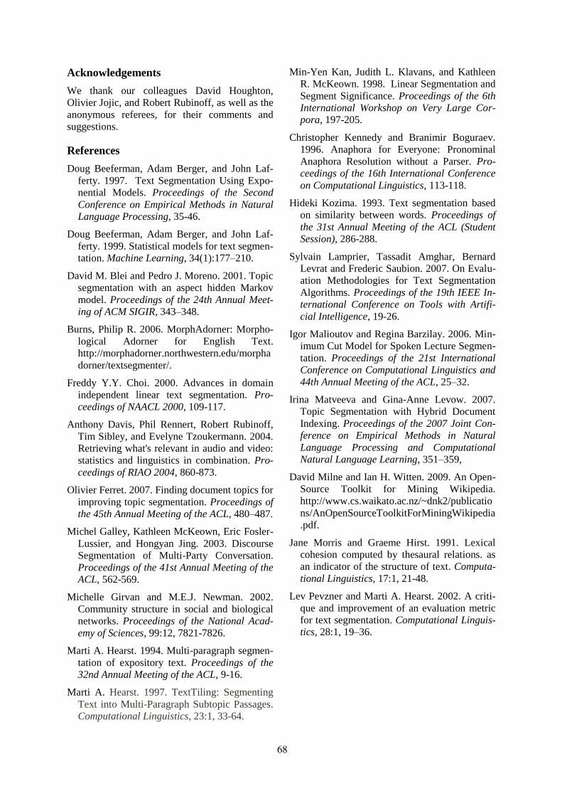
Acknowledgements

We thank our colleagues David Houghton,

Olivier Jojic, and Robert Rubinoff, as well as the

anonymous referees, for their comments and

suggestions.

References

Doug Beeferman, Adam Berger, and John Laf-

ferty. 1997. Text Segmentation Using Expo-

nential Models. Proceedings of the Second

Conference on Empirical Methods in Natural

Language Processing, 35-46.

Doug Beeferman, Adam Berger, and John Laf-

ferty. 1999. Statistical models for text segmen-

tation. Machine Learning, 34(1):177–210.

David M. Blei and Pedro J. Moreno. 2001. Topic

segmentation with an aspect hidden Markov

model. Proceedings of the 24th Annual Meet-

ing of ACM SIGIR, 343–348.

Burns, Philip R. 2006. MorphAdorner: Morpho-

logical Adorner for English Text.

http://morphadorner.northwestern.edu/morpha

dorner/textsegmenter/.

Freddy Y.Y. Choi. 2000. Advances in domain

independent linear text segmentation. Pro-

ceedings of NAACL 2000, 109-117.

Anthony Davis, Phil Rennert, Robert Rubinoff,

Tim Sibley, and Evelyne Tzoukermann. 2004.

Retrieving what's relevant in audio and video:

statistics and linguistics in combination. Pro-

ceedings of RIAO 2004, 860-873.

Olivier Ferret. 2007. Finding document topics for

improving topic segmentation. Proceedings of

the 45th Annual Meeting of the ACL, 480–487.

Michel Galley, Kathleen McKeown, Eric Fosler-

Lussier, and Hongyan Jing. 2003. Discourse

Segmentation of Multi-Party Conversation.

Proceedings of the 41st Annual Meeting of the

ACL, 562-569.

Michelle Girvan and M.E.J. Newman. 2002.

Community structure in social and biological

networks. Proceedings of the National Acad-

emy of Sciences, 99:12, 7821-7826.

Marti A. Hearst. 1994. Multi-paragraph segmen-

tation of expository text. Proceedings of the

32nd Annual Meeting of the ACL, 9-16.

Marti A. Hearst. 1997. TextTiling: Segmenting

Text into Multi-Paragraph Subtopic Passages.

Computational Linguistics, 23:1, 33-64.

Min-Yen Kan, Judith L. Klavans, and Kathleen

R. McKeown. 1998. Linear Segmentation and

Segment Significance. Proceedings of the 6th

International Workshop on Very Large Cor-

pora, 197-205.

Christopher Kennedy and Branimir Boguraev.

1996. Anaphora for Everyone: Pronominal

Anaphora Resolution without a Parser. Pro-

ceedings of the 16th International Conference

on Computational Linguistics, 113-118.

Hideki Kozima. 1993. Text segmentation based

on similarity between words. Proceedings of

the 31st Annual Meeting of the ACL (Student

Session), 286-288.

Sylvain Lamprier, Tassadit Amghar, Bernard

Levrat and Frederic Saubion. 2007. On Evalu-

ation Methodologies for Text Segmentation

Algorithms. Proceedings of the 19th IEEE In-

ternational Conference on Tools with Artifi-

cial Intelligence, 19-26.

Igor Malioutov and Regina Barzilay. 2006. Min-

imum Cut Model for Spoken Lecture Segmen-

tation. Proceedings of the 21st International

Conference on Computational Linguistics and

44th Annual Meeting of the ACL, 25–32.

Irina Matveeva and Gina-Anne Levow. 2007.

Topic Segmentation with Hybrid Document

Indexing. Proceedings of the 2007 Joint Con-

ference on Empirical Methods in Natural

Language Processing and Computational

Natural Language Learning, 351–359,

David Milne and Ian H. Witten. 2009. An Open-

Source Toolkit for Mining Wikipedia.

http://www.cs.waikato.ac.nz/~dnk2/publicatio

ns/AnOpenSourceToolkitForMiningWikipedia

.pdf.

Jane Morris and Graeme Hirst. 1991. Lexical

cohesion computed by thesaural relations. as

an indicator of the structure of text. Computa-

tional Linguistics, 17:1, 21-48.

Lev Pevzner and Marti A. Hearst. 2002. A criti-

que and improvement of an evaluation metric

for text segmentation. Computational Linguis-

tics, 28:1, 19–36.

68

Proceedings of the 2010 Workshop on Graph-based Methods for Natural Language Processing, ACL 2010, pages 69–73,Uppsala, Sweden, 16 July 2010. c©2010 Association for Computational Linguistics

MuLLinG: multilevel linguistic graphs for knowledge extraction

Vincent ArcherLaboratoire I3S (équipe RL), Université de Nice Sophia Antipolis

Sophia Antipolis, Francevincent.archer@unice.fr

Abstract

MuLLinG is a model for knowledge extrac-tion (especially lexical extraction from cor-pora), based on multilevel graphs. Its aim is to allow large-scale data acquisition, by mak-ing it easy to realize automatically, and simple to configure by linguists with limited knowledge in computer programming. In MuLLinG, each new level represents the in-formation in a different manner (more and more abstract). We also introduce several as-sociated operators, written to be as generic as possible. They are independent of what nodes and edges represent, and of the task to achieve. Consequently, they allow the de-scription of a complex extraction process as a succession of simple graph manipulations. Fi-nally, we present an experiment of colloca-tion extraction using MuLLinG model.

1 Introduction

Natural language processing systems often pro-duce low-quality results, because of ambiguities and particular linguistic phenomena. One major reason is the lack of linguistic data needed to de-tect these phenomena or to solve ambiguities. To fill this lack, new linguistic resources should be produced. It could be done quickly with automat-ic processes, but quality would be unsatisfactory; on the contrary, manual work by linguists allows precise results, but takes lot of time. To get both rapidity and precision, we must combine ma-chine and human abilities, by giving automatic processing tools to linguists, and allowing them to guide the process. Existing tools are often too centered on a task, and require too much know-ledge in computer programming: they are not ap-propriate for linguists with few knowledge in coding. We should thus develop generic tools.

In this article, we first focus on how to make the resource gathering easier. Then, we introduce

MuLLinG, our multilevel graph model for lin-guistic extraction, with several associated opera-tions. Finally, we present an application of that model on collocation extraction.

2 Knowledge extraction

There are several manners to collect resources with automatic processes (machine learning, col-laborative interfaces, etc.). We focus here on (lin-guistic and statistic) extraction of candidates. More precisely, our goal is to facilitate the large-scale production of candidates by extraction.

2.1 Simplify programming

Making a particular extraction task is not easy, as there is often no dedicated tool. It forces to write ad hoc tools (most of the time not unveiled). Moreover, ad hoc tools are not written to be uni-versal. They generally depend on the data model, it is therefore difficult or impossible to use a new resource with a different format (such as an ana-lysis from an other parser). To be really useful, an extraction tool should be generic (able to handle different data models) and easy to under-stand and to use. The data model on which the tool rely must be simple, expressive (complex structure should be represented easily), and uni-versal (for monolingual or multilingual corpora, dictionaries, etc.). It should also provide simple generic, task-independent, high-level operations that can be combined to describe a complex task.

We choose to introduce a graph-based model. Graphs are understandable quickly by humans, easy to use in automatic processes, and flexible enough to represent various data types. Using graphs for knowledge extraction is quite classic. They can represent relations between words (pro-duced by dependency analysers from corpora), and be used to produce semantically close terms (Widdows & Dorrow, 2002) or to group similar n-tuples (Hassan et al., 2006). Graphs also can be

69

generated from dictionaries, and used to produce knowledge bases (Richardson et al., 1998) or proximity information (Gaume et al., 2006).

2.2 Existing graph models

Influenced by “existential graphs” (Peirce, 1931-1935) where relations between elements are rep-resented by nodes, “conceptual graphs” (Sowa, 1976) are bipartite graphs with two node types: concepts and conceptual relations (edges only as-sociate relations and concepts). That relation ma-terialization is useful, as it allows to handle eas-ily n-ary relations, without hypergraphs.

Another interesting network is the “lexical system” one (Polguère, 2006), defined as ori-ented, weighted, unhierarchical and, above all, heterogeneous: there is no constraint on what is modelized (it could be terms, meanings, colloca-tions, etc.). It avoids the separation between dic-tionary-like and network-like lexical databases, and shows the same representation can be used for each kind of data and relation.

Finally, graphs can be multilevel, to represent different kinds of information. Links are gener-ally allowed only in a same level or between two adjacent levels, like in “hypertexts” (Agosti and Crestani, 1993) made of three specified levels (documents, terms, concepts), or in Multi-Level Association Graphs (Witschel, 2007) in which there is no constraint on the number of levels. We believe that the use of several levels to rep-resent various content types is pertinent in an ex-traction process, as it allows to handle both the occurrences of terms, and the terms themselves.

3 MuLLinG model

We introduce MuLLinG (Multi-Level Linguistic Graph), our own graph model. Divided in several ordered and distinct levels, it contains two kinds of edges: intra-level ones (between nodes from same level) and inter-level ones (from a node on level i to a node on level i+1). Intra-level edges are not unique (several edges are allowed between two nodes): every level is a multigraph. On the contrary, a node can be the source of only one inter-level edge; this association means that the target node (on the superior level) is a more global representation of the source node (it defines a hierarchy of precision).

Finally, in order to allow the heterogeneity of represented data, nodes and intra-level edges can carry any attribute (with no limit on kind or num-ber). Figure 1 shows an example of a MuLLinG graph, in which 1st level contains occurrences of

words, 2nd level contains lemmas, and 3rd level contains synonymy classes.

3.1 Definition

More precisely, a MuLLinG graph is an oriented multigraph ( )EV

n a,aΦ,A,F,E,V,=G (for n levels) where:

• V: set of nodes, made of n disjoint sub-sets nVV ,,1 … (for the n levels);

• E: set of intra-level edges, made of n dis-joint subsets nEE ,,1 … ; A: set of functions

{ }niVVE iiii ,,1: ∈×→α associating an edge and its two extremities;

• F: set of inter-level edges, in n-1 disjoint sets 11 ,, −… nFF defined as

( ){ }x=y|VVyx,=F +iii ϕ1×∈ ; Φ : set of functions { }niVV +iii ,,1: 1 ∈→ϕ , as-sociating a node (on a given level) and a node on the superior level);

• { }VV ΣVf=a →: , { }EE ΣEf=a →:( EV Σ,Σ are alphabets for attributes of objects from E and V) model attributes.

3.2 Associated operators

To manipulate MuLLinG graphs, we introduce several operations, designed for their particular structure. Some of them allow elementary ma-nipulations: add or delete a node or an edge, clean a node (delete all edges of which it is a source or a target), delete a node and its “des-cendants” (the nodes linked to it by inter-level edges, and their own descendants). There are

Figure 1. Example of 3-level MuLLinG graph

70

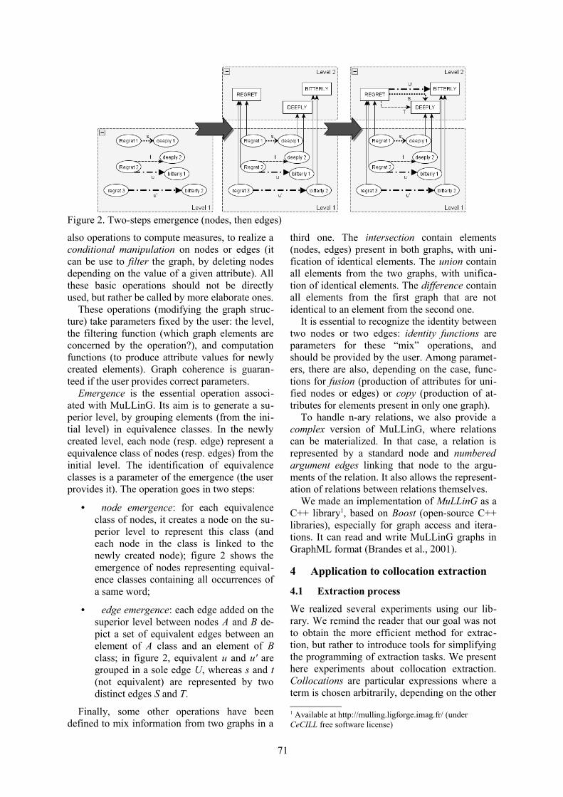
also operations to compute measures, to realize a conditional manipulation on nodes or edges (it can be use to filter the graph, by deleting nodes depending on the value of a given attribute). All these basic operations should not be directly used, but rather be called by more elaborate ones.

These operations (modifying the graph struc-ture) take parameters fixed by the user: the level, the filtering function (which graph elements are concerned by the operation?), and computation functions (to produce attribute values for newly created elements). Graph coherence is guaran-teed if the user provides correct parameters.

Emergence is the essential operation associ-ated with MuLLinG. Its aim is to generate a su-perior level, by grouping elements (from the ini-tial level) in equivalence classes. In the newly created level, each node (resp. edge) represent a equivalence class of nodes (resp. edges) from the initial level. The identification of equivalence classes is a parameter of the emergence (the user provides it). The operation goes in two steps:

• node emergence: for each equivalence class of nodes, it creates a node on the su-perior level to represent this class (and each node in the class is linked to the newly created node); figure 2 shows the emergence of nodes representing equival-ence classes containing all occurrences of a same word;

• edge emergence: each edge added on the superior level between nodes A and B de-pict a set of equivalent edges between an element of A class and an element of B class; in figure 2, equivalent u and u' are grouped in a sole edge U, whereas s and t (not equivalent) are represented by two distinct edges S and T.

Finally, some other operations have been defined to mix information from two graphs in a

third one. The intersection contain elements (nodes, edges) present in both graphs, with uni-fication of identical elements. The union contain all elements from the two graphs, with unifica-tion of identical elements. The difference contain all elements from the first graph that are not identical to an element from the second one.

It is essential to recognize the identity between two nodes or two edges: identity functions are parameters for these “mix” operations, and should be provided by the user. Among paramet-ers, there are also, depending on the case, func-tions for fusion (production of attributes for uni-fied nodes or edges) or copy (production of at-tributes for elements present in only one graph).

To handle n-ary relations, we also provide a complex version of MuLLinG, where relations can be materialized. In that case, a relation is represented by a standard node and numbered argument edges linking that node to the argu-ments of the relation. It also allows the represent-ation of relations between relations themselves.

We made an implementation of MuLLinG as a C++ library1, based on Boost (open-source C++ libraries), especially for graph access and itera-tions. It can read and write MuLLinG graphs in GraphML format (Brandes et al., 2001).

4 Application to collocation extraction

4.1 Extraction process

We realized several experiments using our lib-rary. We remind the reader that our goal was not to obtain the more efficient method for extrac-tion, but rather to introduce tools for simplifying the programming of extraction tasks. We present here experiments about collocation extraction. Collocations are particular expressions where a term is chosen arbitrarily, depending on the other

1 Available at http://mulling.ligforge.imag.fr/ (under CeCILL free software license)

Figure 2. Two-steps emergence (nodes, then edges)

71

term, to express a particular meaning (like in “driving rain”, where “driving” is used to express intensity). As the choice differs between lan-guages2, it causes big issues to machine transla-tion systems (which lack resources to handle them correctly). In our experiment, the initial graph is made of relations produced by a depend-ency analyzer, on 1st level.

Firstly, we use the filtering operator to keep only pertinent relations (nouns modified by ad-jectives, like in figure 3, or verbs modified by adverbs), according to the analyzer. There are re-lations between term occurrences on 1st level, but we want relations between terms themselves: we generate them on 2nd level using emergence. So we proceed node emergence by considering that nodes with same attribute “lemma” are equival-ent, then edge emergence by considering that edges expressing a modification are equivalent.

The “collocation” candidates are all 2nd-level edges created during the emergence. To rank them, we use the computation operation (with occurrence and co-occurrence frequencies) to fix an association measure on those nodes. Figure 3 shows an example of a MuLLinG graph after emergence and computation operations.

To facilitate the description, our library con-tains lots of pre-defined generic functions. By example, a filter (used as a parameter of emer-gence) can be based on an excepted value, a threshold, etc. We also described numerous asso-ciation measures; for now, new ones should be written in the C++ program.

We used our library to carry out the extraction as described previously, with LeMonde95 corpus (news articles) analyzed by Xerox's XIP parser. Thanks to MuLLinG structure, it is very easy to get all potential collocations (heavy/driving rain): these are the relations of which it is the source.2By example, a “heavy smoker” is big in French (“gros fumeur”) and strong in German (“starker Raucher”).

Experiments verb-adverb noun-adjective

Level 1 nodes 1 155 824 1 319 474edges 1 780 759 2 009 051

Level 2 nodes 6 813 33 132edges 144 586 273 655

Table 1. Nodes and edges produced during ex-periments on collocation extraction

4.2 Advantages and drawbacks

With MuLLinG library, we reproduced exactly some experiments on collocation extraction we made before (with ad hoc programs): results are obviously coherent. The production is currently slightly slower (around 20% more time) but speed is not crucial, and could be optimized. MuLLinG has a great advantage while writing the program: it only calls functions (and declare parameters). Consequently, task description with our library is much faster (source lines of code are divided by 5), it also avoids errors. It requires less knowledge in programming, so it is far more accessible. Nevertheless, usability should still be improved: we must describe a high-level lan-guage (we believe it should be a request one). Furthermore, there is no constraint on input re-sources, so programs could easily be re-used with other relations (from other parsers). Finally, as graphs with millions of elements can reach RAM limits, we plan to allow database storage.

We also made bilingual experiments on col-locations, taking advantage of MuLLinG com-plex version to materialize monolingual “colloc-ation” nodes, and to describe bilingual relations between collocations as edges between them.

5 Conclusion

Facing the lack of tools for extraction of lexical knowledge, we looked for a new one, simple and generic. We specified MuLLinG, multilevel graph model (with no constraint on the data), as-sociated with several simple manipulation opera-tions (which could be combined to realize com-plex tasks). The ensuing tool allows to program linguistic tasks in a resource-independent man-ner, simpler and more efficient. One major pro-spect of this work concerns its implementation. As explained before, we must provide a high-level language. It is also necessary to facilitate the import and to optimize memory management. In order to provide a less NLP-centered tool, we should extend it with new operations, and with algorithms related to classic problems of graph theory. It would also be interesting to interact with semantic web tools (RDF/SPARQL).

Figure 3. Collocations extraction with emergence (on 2nd level) and computation operations

72

ReferencesMaristella Agosti and Fabio Crestani. 1993. A Meth-

odology for the Automatic Construction of a Hy-pertext for Information Retrieval. In Proceedings of 1993 ACM Symposium on Applied Computing, 745-753.

Ulrik Brandes, Markus Eiglsperger, Ivan Herman, Mi-chael Himsolt and M. Scott Marshall. 2001. GraphML Progress Report - Structural Layer Pro-posal. In Proceedings of 9th International Sym-posium Graph Drawing (GD'01), 501-512.

Hany Hassan, Ahmed Hassan and Sara Noeman. 2006. Graph based semi-supervised approach for information extraction. In Proceedings of HLT-NAACL-07 Workshop on Textgraphs-06, 9-16.

Bruno Gaume, Karine Duvignau and Martine Van-hove. 2008. Semantic associations and confluences in paradigmatic networks. In Martine Vanhove (Ed.), From Polysemy to Semantic Change To-wards a typology of lexical semantic associations, John Benjamins, 233-264.

Charles Sanders Peirce. 1931-1935. Collected Papers of C. S. Peirce (C. Hartshorne & P. Weiss, eds.), Cambridge: Harvard University Press.

Alain Polguère. 2006. Structural Properties of Lexical Systems: Monolingual and Multilingual Perspect-ives. In Proceedings of Workshop on Multilingual Language Resources and Interoperability (COL-ING/ACL 2006), 50-59.

Stephen D. Richardson, William B. Dolan, and Lucy Vanderwende. 1998. MindNet: acquiring and structuring semantic information from text. In Pro-ceedings of COLING 1998. 1098-1102.

John F. Sowa. 1976. Conceptual graphs for a database interface. IBM Journal of Research and Develop-ment 20:4, 336-357.

Dominic Widdows and Beate Dorow. 2002. A Graph Model for Unsupervised Lexical Acquisition. In Proceedings of 19th International Conference on Computational Linguistics(COLING 2002). 1093-1099.

Hans Friedrich Witschel. 2007. Multi-level Associ-ation Graphs - A New Graph-Based Model for In-formation Retrieval. In Proceedings of HLT-NAACL-07 Workshop on Textgraphs-07, 9-16.

73

Proceedings of the 2010 Workshop on Graph-based Methods for Natural Language Processing, ACL 2010, pages 74–82,Uppsala, Sweden, 16 July 2010. c©2010 Association for Computational Linguistics

Experiments with CST-based Multidocument Summarization

Maria Lucía del Rosario Castro Jorge, Thiago Alexandre Salgueiro Pardo

Núcleo Interinstitucional de Lingüística Computacional (NILC)

Instituto de Ciências Matemáticas e de Computação, Universidade de São Paulo

Avenida Trabalhador são-carlense, 400 - Centro

P.O.Box 668. 13560-970, São Carlos/SP, Brazil

{mluciacj,taspardo}@icmc.usp.br

Abstract

Recently, with the huge amount of growing

information in the web and the little

available time to read and process all this

information, automatic summaries have

become very important resources. In this

work, we evaluate deep content selection

methods for multidocument summarization

based on the CST model (Cross-document

Structure Theory). Our methods consider

summarization preferences and focus on the

overall main problems of multidocument

treatment: redundancy, complementarity, and

contradiction among different information

sources. We also evaluate the impact of the

CST model over superficial summarization

systems. Our results show that the use of

CST model helps to improve informativeness

and quality in automatic summaries.

1 Introduction

In the last years there has been a considerable

increase in the amount of online information and

consequently the task of processing this

information has become more difficult. Just to

have an idea, recent studies conducted by IDC

showed that 800 exabytes of information were

produced in 2009, and it is estimated that in 2012

it will be produced 3 times more. Among all of

this information, there is a lot of related content

that comes from different sources and that

presents similarities and differences. Reading

and dealing with this is not straightforward. In

this scenario, multidocument summarization has

become an important task.

Multidocument summarization consists in

producing a unique summary from a set of

documents on the same topics (Mani, 2001). A

multidocument summary must contain the most

relevant information from the documents. For

example, we may want to produce a

multidocument summary from all the documents

telling about the recent world economical crisis

or the terrorism in some region. As an example,

Figure 1 reproduces a summary from Radev and

Mckeown (1998), which contains the main facts

from 4 news sources.

Figure 1: Example of multidocument summary

(Radev and Mckeown, 1998, p. 478)

Multidocument summarization has to deal not

only with the fact of showing relevant

information but also with some multidocument

phenomena such as redundancy,

complementarity, contradiction, information

ordering, source identification, temporal

resolution, etc. It is also interesting to notice that,

instead of only generic summaries (as the one in

the example), summaries may be produced

considering user preferences. For example, one

may prefer summaries including information

attributed to particular sources (if one trusts more

in some sources) or more context information

(considering a reader that has not accompanied

some recent important news), among other

possibilities.

Reuters reported that 18 people were killed in a

Jerusalem bombing Sunday. The next day, a bomb

in Tel Aviv killed at least 10 people and wounded

30 according to Israel radio. Reuters reported that

at least 12 people were killed and 105 wounded.

Later the same day, Reuters reported that the

radical Muslim group Hamas had claimed

responsibility for the act.

74

There are two main approaches for

multidocument summarization (Mani and

Maybury, 1999): the superficial and the deep

approaches. Superficial approach uses little

linguistic knowledge to produce summaries. This

approach usually has low cost and is more

robust, but it produces poor results. On the other

hand, deep approaches use more linguistic

knowledge to produce summaries. In general

terms, in this approach it is commonly used

syntactical, semantic and discourse parsers to

analyze the original documents. A very common

way to analyze documents consists in

establishing semantic relations among the

documents parts, which helps identifying

commonalities and differences in information.

Within this context, discourse models as CST

(Cross-document Structure Theory) (Radev,

2000) are useful (see, e.g., Afantenos et al.,

2004; Afantenos, 2007; Jorge and Pardo, 2009,

2010; Radev and Mckeown, 1998; Radev et al.,

2001; Zhang et al., 2002).

It was proposed in Mani and Maybury (1999)

a general architecture for multidocument

summarization, with analysis, transformation,

and synthesis stages. The first stage consists in

analyzing and formally representing the content

of the original documents. The second stage

consists mainly in transforming the represented

content into a condensed content that will be

included in the final summary. One of the most

important tasks in this stage is the content

selection process, which consists in selecting the

most relevant information. Finally, the third

stage expresses the condensed content in natural

language, producing the summary.

In this paper, we explore a CST-based

summarization method and evaluate the

corresponding prototype system for

multidocument summarization. Our system,

called CSTSumm (CST-based SUMMarizer),

produces multidocument summaries from input

CST-analyzed news documents. We mainly

investigate content selection methods for

producing both generic and preference-based

summaries. Particularly, we formalize and codify

our content selection strategies as operators that

perform the previously cited transformation

stage. We run our experiments with Brazilian

Portuguese news texts (previously analyzed

according to CST by human experts) and show

that we produce more informative summaries in

comparison with some superficial summarizers

(Pardo, 2005; Radev et al., 2000). We also use

CST to enrich these superficial summarizers,

showing that the results also improve. Our

general hypothesis for this work is that the deep

knowledge provided by CST helps to improve

information and quality in summaries.

This work is organized as follows. In Section

2, the main concepts of the CST model are

introduced and the works that have already used

CST for multidocument summarization are

reviewed. In Section 3, we present CSTSumm,

while its evaluation is reported in Section 4.

Some final remarks are presented in Section 5.

2 Related Work

2.1 Cross-document Structure Theory

Radev (2000) proposed CST model with a set of

24 relations for multidocument treatment in any

domain. Table 1 lists these relations.

Table 1: CST original relations

Identity Judgment

Equivalence Fulfillment

Translation Description

Subsumption Reader profile

Contradiction Contrast

Historical background Parallel

Modality Cross-reference

Attribution Citation

Summary Refinement

Follow-up Agreement

Elaboration Generalization

Indirect speech Change of perspective

The established relations may have (or not)

directionality, e.g., the equivalence relation

(which states that two text segments have similar

content) has no directionality while the historical

background relation (which states that a segment

provides historical information about other) has.

Figure 2 shows examples of these two relations

among sentences from different sources.

As part of the model, the author proposes a

general schema that reveals the possibility of

relationship at any level of linguistic analysis.

Figure 3 (reproduced from Radev, 2000)

illustrates this schema. According to this schema,

the documents with CST relations are

represented as a graph, whose nodes are text

segments (of possibly any level) and the edges

are relations. This graph is possibly

disconnected, since not all segments present

relations with other segments. It is important to

say that, in general, only one analysis level is

treated. In this work, we only deal with sentences

from the input documents, since sentences are

75

well delimited and are standard segments in

discourse analysis.

Figure 2: Examples of CST relations

Figure 3: CST general schema (Radev, 2000, p. 78)

2.2 Multidocument Summarization

A few works explored CST for multidocument

summarization. A 4-stage multidocument

summarization methodology was proposed in

Radev (2000). In this methodology, the first

stage consists in clustering documents according

to their topics. In the second stage, internal

analysis (syntactical and semantic, for instance)

of the texts may be performed. In the third stage,

CST relations are established among texts.

Finally, in the fourth stage, information is

selected to produce the final summary. For this

methodology the author suggests using operators

activated by user summarization preferences

such as authorship (i.e., reporting the information

sources) or contradictory information preference.

The author also says that it may be possible to

produce generic summaries without considering

a particular preference. In this case the criterion

used to select information is based on the number

of CST relations that a segment has. This

criterion is based on the idea that relevant

information is more repeated/elaborated and

related to other segments across documents. This

may be easily verified in practice. In this paper

we follow such ideas.

A methodology for enriching multidocument

summaries produced by superficial summarizers

was proposed by Zhang et al. (2002). The

authors incorporated the information given by

CST relations to MEAD (Radev et al., 2000)

summarization process, showing that giving

preference to segments with CST relations

produces better summaries. Otterbacher et al.

(2002) investigated how CST relations may

improve cohesion in summaries, which was

tested by ordering sentences in summaries

according to CST relations. The idea used behind

this ordering is that sentences related by CST

relations should appear closer in the final

summaries as well as should respect possible

temporal constraints indicated by some relations.

Afantenos et al. (2004) proposed another

summarization methodology that extracts

message templates from the texts (using

information extraction tools) and, according to

the type of CST relation between two templates,

produces a unified message that would represent

the summary content. The authors did not fully

implement this method.

3 CSTSumm

In this paper we evaluate a CST-based

multidocument summarization method by

implementing and testing a prototype system,

called CSTSumm. It performs content selection

operations over a group of texts on the same

topic that were previously annotated according to

CST. For the moment, we are using manually

annotated texts, i.e., the analysis stage of

multidocument summarization is only simulated.

In the future, texts may be automatically

annotated, since a CST parser is under

development for Brazilian Portuguese language

(Maziero et al., 2010).

Initially, the system receives as input the

CST-annotated texts, which are structured as a

graph. An initial rank of sentences is then built:

the sentences are ordered according to the

number of CST relations they present; the more

Equivalence relation

Sentence 1: Nine people died, three of them

children, and 25 others were wounded last

Monday in a blast at a market in Moscow,

police said.

Sentence 2: Nine people died, including three

children, and 25 others were injured last

Monday in an explosion that happened at a

market in Moscow, police of Moscow

informed.

Historical background relation

(directionality: from Sentence 2 to 1)

Sentence 1: An airplane accident in Bukavu,

east of Democratic Republic of Congo, killed

13 people this Thursday in the afternoon.

Sentence 2: Congo has a history of more than

30 airplane tragedies.

76

relations a sentence presents, better ranked it will

be. Having the initial rank, content selection is

performed. In this work, following the idea of

Jorge and Pardo (2010), we represent and codify

each content selection strategy as an operator. A

content selection operator tells how to rearrange

the sentences in the rank in order to produce

summaries that better satisfy the corresponding

user preferences. For instance, if a user requires

more context information in the summary, the

corresponding operator is activated. Such

operator will (i) select in the rank all the

sentences that present historical background and

elaboration CST relations with better ranked

sentences and (ii) improve their position in the

rank by putting them immediately after the better

ranked sentences with which they are related.

This final action would give to these

“contextual” sentences more preference for being

in the summary, since they are better positioned

in the refined rank. Figure 4 shows an example

of a hypothetical CST graph (derived from a

group of texts), the corresponding initial rank

(with relations preserved for clarification) and

the transformation that the context operator

would do for producing the new/refined rank. It

is possible to see that sentence 1, that presents

historical information about the sentence 4, gets

a better position in the rank (immediately after

sentence 4), receiving some privilege to be in the

summary.

Besides the context operator, we also have

other 3 operators: the contradiction operator

(which looks for the contradiction CST relation

in order to include in the summary every

contradiction in the texts), the authorship

operator (which looks for the citation and

attribution CST relations in order to include in

the summary possible sources that provided the

available information), and the evolving events

operator (which looks for historical background

and follow-up CST relations in order to present

the development of the events during a time

period).

Independently from the user preference, an

extra operator is always applied: the redundancy

operator. It removes from the rank all sentences

whose information is already expressed in other

better ranked sentences. Redundancy is

represented by the identity, equivalence, and

subsumption CST relations.

After the content selection process, in the last

stage – the synthesis stage – the system selects as

many sentences from the rank as allowed by the

specified compression rate. The compression rate

(provided by the user) informs the size of the

summary. For instance, a 70% rate indicates that

the summary must have at most 30% of the

number of words in a text. In this work, given the

multidocument nature of the task, we compute

the compression rate over the size of the longest

text in the group.

Hypothetical CST graph

Initial rank

Refined rank (after applying the operator)

Figure 4: Example of context operator application

Synthesis stage also orders the selected sentences

according to a simple criterion that only

considers the position of the sentences in the

original documents: first sentences appear first in

the summary. If two sentences have the same

position but in different documents, then the

sentences are ordered according to the document

number. Finally, we apply a sentence fusion

system (Seno and Nunes, 2009) to some selected

sentences. This is done when sentences with

overlap CST relation among them are selected to

the summary. The overlap relation indicates that

the sentences have similar content, but also that

both present unique content. In this case, it is

desired that the sentences become only one with

the union of their contents. The fusion system

that we use does that. Figure 5 illustrates the

fusion process, with the original sentences and a

resulting fusion.

Figure 6 shows the general architecture of

CSTSumm, which summarizes the whole process

described before. Each operator is codified in

77

XML, where it is specified which relations

should be looked in the rank in order to have the

correspondent sentences better ranked. It is

important to notice that, excepting the

redundancy operator, our system was designed to

allow the application of only one content

selection operator at a time. If more than one

operator is applied, the application of the

following operator may probably rewrite the

modifications in the rank that the previous

operator has done. For instance, the application

of the contradiction operator after the context

operator might include sentences with

contradiction above sentences with context

information in the rank, altering therefore the

rank produced by the context operator. One

simple alternative to this design choice is to ask

the user to rank his preferences and, then, to

apply the corresponding operators in the opposite

order, so that the rank produced by the most

important preference will not be further altered.

Other alternative is to produce more complex

operators that combine preferences (and the

corresponding CST relations), but some

preference on the relations should still be

specified.

Figure 5: Example of sentence fusion

Figure 6: CSTSumm architecture

In Figure 7 we show the algorithm for the

application of operators during content selection

process. It is important to notice that the selected

operator looks for its relations in all pairs of

sentences in the rank. Once it finds the relations,

it rearranges the rank appropriately, by putting

the related sentence more above in the rank.

Figure 7: Algorithm for application of content

selection operators

As an illustration of the results of our system,

Figure 8 shows an automatic summary produced

from a group of 3 texts with the application of

the context operator (after redundancy operator

was applied) and a 70% compression rate. The

summary was translated from Portuguese, the

language with which the summarizer was tested.

Figure 8: Example of multidocument summary with

context information

4 Evaluation

Our main research question in this work was how

helpful CST would be for producing better

summaries. CSTSumm enables us to assess the

summaries and content selection strategies, but a

comparison of these summaries with summaries

produced by superficial methods is still

necessary. In fact, we not only proceeded to such

Sentence 1: According to a spokesman from

United Nations, the plane was trying to land at

the airport in Bukavu in the middle of a storm.

Sentence 2: Everyone died when the plane,

hampered by bad weather, failed to reach the

runway and crashed in a forest 15 kilometers

from the airport in Bukavu.

Fusion: According to a spokesman for the United

Nations, everyone died when a plane that was

trying to land at Bukavu airport, hampered by bad

weather, failed to reach the runway and crashed

in a forest 15 kilometers from the airport.

procedure for application of content selection

operators

input data: initial rank, user summarization

preference, operators

output data: refined rank

apply the redundancy operator

select one operator according to the user

summarization preference

for i=sentence at the first position in the rank to the

last but one sentence

for j=sentence at position i+1 in the rank to the

last sentence

if the operator relations happen among

sentences i and j, rearrange the rank

appropriately

The Brazilian volleyball team has won on Friday

the seventh consecutive victory in the World

League, defeating Finland by 3 sets to 0 - partials

of 25/17, 25/22 and 25/21 - in a match in the

Tampere city, Finland. The first set remained

balanced until the middle, when André Heller

went to serve. In the last part, Finland again

paired the game with Brazil, but after a sequence

of Brazilians points Finland failed to respond and

lost by 25 to 21. The Brazilian team has won five

times the World League in 1993, 2001, 2003,

2004 and 2005.

78

comparison, but also improved the superficial

methods with CST knowledge.

As superficial summarizers, we selected

MEAD (Radev et al., 2000) and GistSumm

(Pardo et al., 2003; Pardo, 2005) summarizers.

MEAD works as follows. Initially, MEAD builds

an initial rank of sentences according to a score

based on three parameters: position of the

sentence in the text, lexical distance of the

sentence to the centroid of the text, and the size

of the sentence. These three elements are linearly

combined for producing the score. GistSumm, on

the other side, is very simple: the system

juxtaposes all the source texts and gives a score

to each sentence according to the presence of

frequent words (following the approach of Luhn,

1958) or by using TF-ISF (Term Frequency –

Inverse Sentence Frequency, as proposed in

Larroca et al., 2000). Following the work of

Zhang et al. (2002), we decided to use CST to

rearrange (and supposedly improve) the sentence

ranks produced by MEAD and GistSumm. We

simply add to each sentence score the number of

CST relations that the sentence presents:

new sentence score = old sentence score + number of

CST relations

The number of sentences is retrieved from the

CST graph. This way, the sentence positions in

the rank are changed.

For our experiments, we used the CSTNews

corpus (Aleixo and Pardo, 2008), which is a

corpus of news texts written in Brazilian

Portuguese. The corpus contains 50 clusters of

texts. Each group has from 2 to 4 texts on the

same topic annotated according to CST by

human experts, as well as a manual generic

summary with 70% compression rate (in relation

to the longest text). The annotation process was

carried out by 4 humans, with satisfactory

agreement, which demonstrated that the

annotation task was well defined and performed.

More details about the corpus and its annotation

process are presented by Maziero et al. (2010).

For each cluster of CSTNews corpus, it was

produced a set of automatic summaries

corresponding to each method that was explored

in this work. To evaluate the informativity and

quality of the summaries, we used two types of

evaluation: automatic evaluation and human

evaluation. For the automatic evaluation we used

ROUGE (Lin, 2004) informativity measure,

which compares automatic summaries with

human summaries in terms of the n-grams that

they have in common, resulting in precision,

recall and f-measure numbers between 0 (the

worst) and 1 (the best), which indicate how much

information the summary presents. Precision

indicates the amount of relevant information that

the automatic summary contains; recall indicates

how much information from the human summary

is reproduced in the automatic summary; f-

measure is a unique performance measure that

combines precision and recall. Although it looks

simple, ROUGE author has showed that it

performs as well as humans in differentiating

summary informativeness, which caused the

measure to be widely used in the area. In

particular, for this work, we considered only

unigram comparison, since the author of the

measure demonstrated that unigrams are enough

for differentiating summary quality. For

computing ROUGE, we compared each

automatic summary with the corresponding

human summary in the corpus.

We computed ROUGE for every summary we

produced through several strategies: using only

the initial rank, only the redundancy operator,

and the remaining preference operators (applied

after the redundancy operator). Is is important to

notice that it is only fair to use ROUGE to

evaluate the summaries produced by the initial

rank and by the redundancy operator, since the

human summary (to which ROUGE compares

the automatic summaries) are generic, produced

with no preference in mind. We only computed

ROUGE for the preference-biased summaries in

order to have a measure of how informative they

are. Ideally, these preference-biased summaries

should not only mirror the user preference, but

also contain the main information from the

source texts.

On the other hand, we used human evaluation

to measure the quality of the summaries in terms

of coherence, cohesion and redundancy, factors

that ROUGE is not sensitive enough to capture.

By coherence, we mean the characteristic of a

text having a meaning and being understandable.

By cohesion, we mean the superficial makers of

coherence, i.e., the sequence of text elements that

connect the ideas in the text, as punctuation,

discourse markers, anaphors, etc.

For each one of the above evaluation factors,

a human evaluator was asked to assign one of

five values: very bad (score 0), bad (score 1),

regular (score 2), good (score 3), and excellent

(score 4). We also asked humans to evaluate

informativity in the preference-biased summaries

produced by our system, which is a more fair

79

evaluation than the automatic one described

above. The user should score each summary

(using the same values above) according to how

much he was satisfied with the actual content of

the summary in face of the preference made. The

user had access to the source texts for performing

the evaluation.

Table 2 shows the ROUGE scores for the

summaries produced by the initial rank, by the

application of the operators, by the superficial

summarizers, and by the CST-enriched

superficial summarizers. It is important to say

that these results are the average results obtained

for the automatic summaries generated for all the

clusters in the CSTNews corpus.

Table 2: ROUGE results

Content selection method Precision Recall F-measure

Initial rank 0.5564 0.5303 0.5356

Redundancy treatment (only) 0.5761 0.5065 0.5297

Context information 0.5196 0.4938 0.4994

Authorship information 0.5563 0.5224 0.5310

Contradiction information 0.5503 0.5379 0.5355

Evolving events information 0.5159 0.5222 0.5140

MEAD without CST 0.5242 0.4602 0.4869

MEAD with CST 0.5599 0.4988 0.5230

GistSumm without CST 0.3599 0.6643 0.4599

GistSumm with CST 0.4945 0.5089 0.4994

As expected, it may be observed that the best

results were achieved by the initial rank (since it

produces generic summaries, as happens to the

human summaries to which they are compared),

which does not consider any summarization

preference at all. It is also possible to see that: (a)

the superficial summarizers are outperformed by

the CST-based methods and (b) CST-enriched

superficial summarizers produced better results

than the superficial summarizers.

Results for human evaluation are shown in

Table 3. These results show the average value for

each factor evaluated for a sample group of 48

texts randomly selected from the corpus. We also

associated to each value the closest concept in

our evaluation. We could not perform the

evaluation for the whole corpus due to the high

cost and time-demanding nature of the human

evaluation. Six humans carried out this

evaluation. Each human evaluated eight

summaries, and each summary was evaluated by

three humans.

Table 3: Results for human evaluation

Content selection method Coherence Cohesion Redundancy Informativity

Initial rank 3.6

Excellent

3.2

Good

1.8

Regular

3.6

Excellent

Context 2.1

Regular

2.7

Good

3.6

Excellent

2.2

Regular

Authorship

3.3

Good

2.4

Regular

2.8

Good

3

Good

Contradiction 2.4

Regular

2.7

Good

2.5

Regular

3.7

Excellent

Evolving events 2.1

Regular

2.5

Regular

2.6

Good

3.2

Good

It may be observed that informativity factor

results are quite satisfactory, since more than

50% of the judges considered that the

performance was excellent. For coherence,

cohesion and redundancy factors, results were

not excellent in all the cases, but they were not

bad either. We consider that one of the things

that could have had an influence in this case is

the performance of the fusion system, since it

may generate sentences with some problems of

coherence and cohesion. There are also other

things that may influence these results, such as

80

the method for ordering sentences that we used

in this work. This method does not follow any

deep criteria to order sentences and may also

lead to coherence and cohesion problems.

These results show that CSTSumm is capable

of producing summaries with good informativity

and quality. In fact, the results validate our

hypothesis that deep knowledge may improve the

results, since it deals better with the

multidocument phenomena, as the presence of

redundant, complementary and contradictory

information.

5 Final Remarks

Although we consider that very good results

were achieved, there is still room for

improvements. Future works include the

investigation of better sentence ordering

methods, as well as more investigation on how to

jointly apply more than one content selection

operator.

For the moment, CSTSumm assumes that the

texts to be summarized must be already

annotated with CST. In the future, as soon as an

automatic CST parser is available for

Portuguese, it should provide the suitable input

to the summarizer.

Finally, it is interesting to notice that,

although we have tested our methods with

Brazilian Portuguese texts, they are robust and

generic enough to be applied to any other

language, since both our methods and CST

model are language independent.

Acknowledgments

The authors are grateful to FAPESP and CNPq

for supporting this work.

References

Afantenos, S.D.; Doura, I.; Kapellou, E.;

Karkaletsis, V. 2004. Exploiting Cross-

Document Relations for Multi-document

Evolving Summarization. In the Proceedings

of SETN, pp. 410-419.

Afantenos, S.D. 2007. Reflections on the Task of

Content Determination in the Context of

Multi-Document Summarization of Evolving

Events. In Recent Advances on Natural

Language Processing. Borovets, Bulgaria.

Aleixo, P. and Pardo, T.A.S. 2008. CSTNews:

Um Córpus de Textos Journalísticos Anotados

segundo a Teoria Discursiva CST (Cross-

Document Structure Theory). Série de

Relatórios Técnicos do Instituto de Ciências

Matemáticas e de Computação, Universidade

de São Paulo no. 326. São Carlos, Brazil .

Jorge, M.L.C and Pardo, T.A.S. 2009. Content

Selection Operators for Multidocument

Summarization based on Cross-document

Structure Theory. In the Proceedings of the 7th

Brazilian Symposium in Information and

Human Language Technology. São Carlos,

Brazil.

Jorge, M.L.C. and Pardo, T.A.S. 2010.

Formalizing CST-based Content Selection

Operations. In the Proceedings of the 9th

International Conference on Computational

Processing of Portuguese Language (Lecture

Notes in Artificial Intelligence 6001), pp. 25-

29. Porto Alegre, Brazil.

Larocca Neto, J.; Santos, A.D.; Kaestner, A.A.;

Freitas, A.A. 2000. Generating Text

Summaries through the Relative Importance of

Topics. In M.C. Monard and J.S. Sichman

(eds.), Lecture Notes in Artificial Intelligence,

N. 1952, pp. 300-309. Springer, Verlag.

Lin, C-Y. 2004. ROUGE: a Package for

Automatic Evaluation of Summaries. In the

Proceedings of the Workshop on Text

Summarization Branches Out. Barcelona,

Spain.

Luhn, H.P. 1958. The automatic creation of

literature abstracts. IBM Journal of Research

and Development, Vol. 2, pp. 159-165.

Barcelona, Spain.

Mani, I. and Maybury, M. T. 1999. Advances in

automatic text summarization. MIT Press,

Cambridge, MA.

Mani, I. 2001. Automatic Summarization. John

Benjamins Publishing Co. Amsterdam.

Maziero, E.G.; Jorge, M.L.C.; Pardo, T.A.S.

2010. Identifying Multidocument Relations. In

the Proceedings of the 7th International

Workshop on Natural Language Processing

and Cognitive Science. June 8-12,

Funchal/Madeira, Portugal.

Otterbacher, J.C.; Radev, D.R.; Luo, A. 2002.

Revisions that improve cohesion in multi-

document summaries: a preliminary study. In

the Proceedings of the Workshop on

Automatic Summarization, pp 27-36.

Philadelphia.

81

Pardo, T.A.S.; Rino, L.H.M.; Nunes, M.G.V.

2003. GistSumm: A Summarization Tool

Based on a New Extractive Method. In N.J.

Mamede, J. Baptista, I. Trancoso, M.G.V.

Nunes (eds.), 6th Workshop on Computational

Processing of the Portuguese Language -

Written and Spoken (Lecture Notes in

Artificial Intelligence 2721), pp. 210-

218. Faro, Portugal.

Pardo, T.A.S. 2005. GistSumm - GIST

SUMMarizer: Extensões e Novas

Funcionalidades. Série de Relatórios do

NILC. NILC-TR-05-05. São Carlos, Brazil.

Radev, D. and McKeown, K. 1998. Generating

natural language summaries from multiple on-

line sources. Computational Linguistics, Vol.

24, N. 3, pp. 469-500.

Radev, D.R. 2000. A common theory of

information fusion from multiple text sources,

step one: Cross-document structure. In the

Proceedings of the 1st ACL SIGDIAL

Workshop on Discourse and Dialogue. Hong

Kong.

Radev, D.R.; Jing, H.; Budzikowska, M. 2000.

Centroid-based summarization of multiple

documents: sentence extraction, utility-based

evaluation and user studies. In the

Proceedings of the ANLP/NAACL Workshop,

pp. 21-29.

Radev, D.R.; Blair-Goldensohn, S.; Zhang, Z.

2001. Experiments in single and multi-

document summarization using MEAD. In the

Proceedings of the 1st Document

Understanding Conference. New Orleans, LA.

Seno, E.R.M. and Nunes, M.G.V. 2009.

Reconhecimento de Informações Comuns para

a Fusão de Sentenças Comparáveis do

Português. Linguamática, Vol. 1, pp. 71-87.

Zhang, Z.; Goldenshon, S.B.; Radev, D.R. 2002.

Towards CST-Enhanced Sumarization. In the

Proceedings of the 18th National Conference

on Artificial Intelligence. Edmonton.

82

Proceedings of the 2010 Workshop on Graph-based Methods for Natural Language Processing, ACL 2010, pages 83–87,Uppsala, Sweden, 16 July 2010. c©2010 Association for Computational Linguistics

Distinguishing between Positive and Negative Opinions with ComplexNetwork Features

Diego R. Amancio, Renato Fabbri, Osvaldo N. Oliveira Jr.,Maria G. V. Nunes and Luciano da F. Costa

University of Sao Paulo, Sao Carlos, Sao Paulo, Brazildiego.amancio@usp.br, renato.fabbri@gmail.com, chu@ifsc.usp.br,

gracan@icmc.usp.br, ldfcosta@gmail.com

Abstract

Topological and dynamic features of com-plex networks have proven to be suitablefor capturing text characteristics in recentyears, with various applications in natu-ral language processing. In this article weshow that texts with positive and negativeopinions can be distinguished from eachother when represented as complex net-works. The distinction was possible byobtaining several metrics of the networks,including the in-degree, out-degree, short-est paths, clustering coefficient, between-ness and global efficiency. For visu-alization, the obtained multidimensionaldataset was projected into a 2-dimensionalspace with the canonical variable analysis.The distinction was quantified using ma-chine learning algorithms, which allowedan recall of 70% in the automatic dis-crimination for the negative opinions, evenwithout attempts to optimize the patternrecognition process.

1 Introduction

The use of statistical methods is well estab-lished for a number of natural language pro-cessing tasks (Manning and Schuetze, 2007), insome cases combined with a deep linguistic treat-ment in hybrid approaches. Representing text asgraphs (Antiqueira et al., 2007), in particular, hasbecome popular with the advent of complex net-works (CN) (Newman, 2003; Albert and Barabasi,2002), especially after it was shown that largepieces of text generate scale-free networks (Ferreri Cancho and Sole, 2001; Barabasi, 2009). Thisscale-free nature of such networks is probably themain reason why complex networks concepts arecapable of capturing features of text, even in theabsence of any linguistic treatment. Significantly,

the scale-free property has also allowed CN to beapplied in diverse fields (Costa et al., 2008), fromneuroscience (Sporns, 2002) to physics (Gfeller,2007), from linguistics (Dorogovtsev and Mendes,2001) to computer science (Moura et al., 2003), tomention a few areas. Other frequently observedunifying principles that natural networks exhibitare short paths between any two nodes and highclustering coefficients (i.e. the so-called small-world property), correlations in node degrees, anda large number of cycles or specific motifs.

The topology and the dynamics of CN can beexploited in natural language processing, whichhas led to several contributions in the literature.For instance, metrics of CN have been used to as-sess the quality of written essays by high schoolstudents (Antiqueira et al., 2007). Furthermore,degrees, shortest paths and other metrics of CNwere used to produce strategies for automatic sum-marization (Antiqueira et al., 2009), whose resultsare among the best for methods that only employstatistics. The quality of machine translation sys-tems can be examined using local mappings of lo-cal measures (Amancio et al., 2008). Other re-lated applications include lexical resources anal-ysis (Sigman and Cecchi, 2002), human-inducedwords association (Costa, 2004), language evolu-tion (Dorogovtsev and Mendes, 2002), and author-ship recognition (Antiqueira et al., 2006).

In this paper, we model texts as complex net-works with each word being represented by anode and co-occurrences of words defining theedges (see next section). Unlike traditional meth-ods of text mining and sentiment detection of re-views (Tang et al., 2009; Pennebaker et al., 2003),the method described here only takes into accountthe relationships between concepts, regardless ofthe semantics related to each word. Specifically,we analyze the topology of the networks in orderto distinguish between texts with positive and neg-ative opinions. Using a corpus of 290 pieces of

83

Before pre-processing After pre-processingThe projection of the projectionnetwork data into two network data twodimensions is crucial dimension be crucial

for big networks big network

Table 1: Adjacency list obtained from the sentence“The projection of the network data into two di-mensions is crucial for big networks”.

text with half of positive opinions, we show thatthe network features allows one to achieve a rea-sonable distinction.

2 Methodology

2.1 Representing texts as complex networks

Texts are modeled as complex networks here byconsidering each word (concept) as a node and es-tablishing links by co-occurrence of words, disre-garding the punctuation. In selecting the nodes,the stopwords were removed and the remainingwords were lemmatized to combine words withthe same canonical form but different inflectionsinto a single node. Additionally, the texts werelabeled using the MXPost part-of-speech Tag-ger based on the Ratnaparki’s model (Ratnaparki,1996), which helps to resolve problems of am-biguity. This is useful because the words withthe same canonical form and same meaning aregrouped into a single node, while words that havethe same canonical form but distinct meaningsgenerate distinct nodes. This pre-processing isdone by accessing a computational lexicon, whereeach word has an associated rule for the genera-tion of the canonical form. For illustrative means,Table 1 shows the pre-processed form of the sen-tence “The projection of the network data into twodimensions is crucial for big networks” and Figure1 shows the network obtained for the same sen-tence.

Several CN metrics have been used to analyzetextual characteristics, the most common of whichare out-degree (kout), in-degree (kin), cluster co-efficient (C) and shortest paths (l). Here we alsouse the betweenness (ϱ) and the global efficiency(η). The out-degree corresponds to the numberof edges emanating from a given node, wherethe weight of each link between any two nodesmay also be considered, being referred to as out-strength. Analogously, the node’s in-degree is de-fined as the number of edges arriving at a given

Figure 1: Network obtained from the sentence“The projection of the network data into two di-mensions is crucial for big networks”.

node. The network’s kout and kin are evaluatedby calculating the average among all the nodes,note that such global measures kout and kin arealways equal. Regarding the adjacency matrix torepresent the network, for a given node i, its kout

and kin are calculated by eqs 1 and 2, where Nrepresents the number of distinct words in the pre-processed text:

kout(i) =N∑

j=1

Wji (1)

kin(i) =N∑

j=1

Wij (2)

The cluster coefficient (C) is defined as follows.Let S be the set formed by nodes receiving edgesof a given node i, and Nc is the cardinality of thisset. If the nodes of this set form a completely con-nected set, then there are Nc(Nc-1) edges in thissub graph. However, if there are only B edges,then the coefficient is given by eq. (3):

C(i) =B

Nc(Nc − 1)(3)

If Nc is less than 1, then C is defined as zero.Note that this measure quantifies how the nodesconnected to a specific node are linked to eachother, with its value varying between zero and one.

The shortest paths are calculated from all pairsof nodes within the network. Let dij be the min-imum distance between any two words i and j inthe network. The shortest path length l of a node iis given in equation 4.

84

l(i) =1

N − 1

∑j =i

dij (4)

Another measure often used in network analy-sis is the global efficiency (η), which is defined inequation 5, and may be interpreted as the speedwith which information is exchanged between anytwo nodes, since a short distance dij contributesmore significantly than a long distance. Note thatthe formula below prevents divergence; therefore,it is especially useful for networks with two ormore components. The inverse of η, named har-monic mean of geodesic distances, has also beenused to characterize complex networks.

η =1

N(N − 1)

∑i=j

1

dij(5)

While l and η use the length of shortest paths,the betweenness uses the number of shortest paths.Formally, the betweenness centrality for a givenvertex v is given in equation 6, where the numera-tor represents the number of shortest paths passingthrough the vertices i, v and j and the denomina-tor represents the number of shortest paths pass-ing through the vertices i and j. In other words,if there are many shortest paths passing through agiven node, this node will receive a high between-ness centrality.

ϱ(v) =∑

i

∑j

σ(i, v, j)

σ(i, j)(6)

2.2 CorpusThe corpus used in the experiments was ob-tained from the Brazilian newspaper Folha de SaoPaulo1, from which we selected 290 articles over a10-year period from a special section where a pos-itive opinion is confronted with a negative opinionabout a given topic. For this study, we selectedthe 145 longest texts with positive opinion and the145 longest text with negative opinions2, in orderto have meaningful statistical data for the CN anal-ysis.

2.3 Machine Learning MethodsIn order to discriminate the topological featuresfrom distinct networks we first applied a techniquefor reducing the dimension of the dataset, thecanonical variable analysis (McLachlan, 2004).

1http://www.folha.com.br2The average size of the selected corpus is 600 words.

The projection of network data into a lower di-mension is crucial for visualization, in additionto avoids the so-called “curse of dimensional-ity” (Bishop, 2006). To calculate the axes pointsfor projecting the data, a criterion must be es-tablished with which the distances between datapoints are defined. Let S be the overall disper-sion of the measurements, as shown in equation 7,where ζ is the number of instances (ζ = 290), −→xc isthe set of metrics for a particular instance and ⟨−→x ⟩is the average of all −→xc.

S =ζ∑

c=1

(−→xc − ⟨−→x ⟩

)(−→xc − ⟨−→x ⟩

)T(7)

Considering that two classes (C1 = positiveopinions and C2 = negative opinions) are used, thescatter matrix Si is obtained for each class Ci, ac-cording to equation 8, where ⟨−→x ⟩i is the analo-gous of ⟨−→x ⟩ when only the instances belonging toclass Ci is taken into account.

Si =∑c∈Ci

(−→xc − ⟨−→x ⟩i

)(−→xc − ⟨−→x ⟩i

)T(8)

The intraclass matrix, i.e. the matrix that givesthe dispersion inside C1 and C2, is defined as inequation 9. Additionally, we define the interclassmatrix, i.e. the matrix that provides the dispersionbetween C1 and C2, as shown in equation 10.

Sintra = S1 + S2 (9)

Sinter = S − Sintra (10)

The principal axes for the projection are thenobtained by computing the eigenvector associ-ated with the largest eigenvalues of the ma-trix Λ (McLachlan, 2004) defined in equation11. Since the data were projected in a two-dimensional space, the two principal axes were se-lected, corresponding to the two largest eigenval-ues.

Λ = S−1intraSinter (11)

Finally, to quantify the efficiency of separa-tion with the projection using canonical variableanalysis, we implemented three machine learn-ing algorithms (decision tree, using the C4.5 algo-rithm (Quinlan, 1993); rules of decision, using the

85

RIP algorithm (Cohen, 1995), and Naive Bayesalgorithm (John and Langley, 1995)) and eval-uated the accuracy rate using the 10-fold-cross-validation (Kohavi, 1995).

3 Results and Discussion

The metrics out-degree (kout), in-degree (kin),shortest paths (l), cluster coefficient (C), between-ness (ϱ) and global efficiency (η) were computedfor each of the 145 texts for positive and nega-tive opinions, as described in the Methodology.The mean values and the standard deviations ofthese metrics were used as attributes for each text.This generated a dataset described in 10 attributes,since the average kin is equal to the average kout

and the standard deviation of η is not defined (inother words, it is always zero). Figure 2 shows theprojection of the dataset obtained with canonicalvariable analysis, illustrating that texts with dif-ferent opinions can be distinguished to a certainextent. That is to say, the topological features ofnetworks representing positive opinion tend to dif-fer from those of texts with negative opinion.

The efficiency of this methodology for charac-terizing different opinions can be quantified usingmachine learning algorithms to process the datafrom the projection. The results are illustrated inTable 2. Again, the distinction between classes isreasonably good, since the accuracy rate reached62%. Indeed, this rate seems to be a good result,since the baseline method3 tested showed an ac-curacy rate of 53%. One also should highlightthe coverage found for the class of negative re-views by using the C4.5 algorithm, for which avalue of 82% (result not shown in the Table 2) wasobtained. This means that if an opinion is nega-tive, the probability of being classified as negativeis only 18%. Thus, our method seems especiallyuseful when a negative view should be classifiedcorrectly.

Method Correctly classifiedC4.5 58%Rip 60%

Naive Bayes 62%

Table 2: Percentage of correctly classified in-stances.

3The baseline method used as attributes the frequency ofeach word in each text. Then, the algorithm C4.5 was runwith the same parameters used for the methodology based oncomplex networks.

-0.120 -0.110 -0.100 -0.090

-0.180

-0.175

-0.170

-0.165

-0.160

-0.155

-0.150

FIRST PRINCIPAL AXIS

SE

CO

ND

PR

INC

IPA

LA

XIS

POSITIVE

NEGATIVE

PROJECTION OF POSITIVE AND

NEGATIVE OBSERVATIONS

Figure 2: Projection obtained by using the methodof canonical variables. A reasonable distinctioncould be achieved between positive and negativeopinions.

4 Conclusion and Further Work

The topological features of complex networksgenerated with texts appear to be efficient in dis-tinguishing between attitudes, as indicated herewhere texts conveying positive opinions could bedistinguished from those of negative opinions.The metrics of the CN combined with a projec-tion technique allowed a reasonable separation ofthe two types of text, and this was confirmed withmachine learning algorithms. An 62% accuracywas achieved (the baseline reached 53%), eventhough there was no attempt to optimize the met-rics or the methods of analysis. These promis-ing results are motivation to evaluate other typesof subtleties in texts, including emotional states,which is presently being performed in our group.

Acknowledgements: Luciano da F. Costais grateful to FAPESP (05/00587-5) and CNPq(301303/06-1 and 573583/2008-0) for the finan-cial support. Diego R. Amancio is grateful toFAPESP sponsorship (proc. 09/02941-1) and Re-nato Fabbri is grateful to CAPES sponsorship. Wealso thank Dr. Oto Araujo Vale very much for sup-plying the corpus.

86

ReferencesC. D. Manning and H. Schuetze. 1999. Foundations of

Statistical Natural Language Processing. The MITPress, First Edition.

L. Antiqueira, M. G. V. Nunes, O. N. Oliveira Jr. and L.da F. Costa. 2007. Strong correlations between textquality and complex networks features. Physica A,373:811–820.

M. E. J. Newman. 2003. The Structure and Functionof Complex Networks. SIAM Review, 45:167–256.

R. Z. Albert and A.L. Barabasi. 2002. Statistical Me-chanics of Complex Networks. Rev. Modern Phys.,74:47–97.

R. Ferrer i Cancho and R. V. Sole. 2001. The smallworld of human language. Proceedings of the RoyalSociety of London B, 268:2261.

A.L. Barabasi. 2009. Scale-Free Networks: a decadeand beyond. Science, 24 325 5939 412–413.

L. F. da Costa, O. N. Oliveira Jr., G. Travieso, F.A. Rodrigues, P. R. Villas Boas, L. Antiqueira, M.P. Viana, L. E. C. da Rocha. 2008. Analyzingand Modeling Real-World Phenomena with Com-plex Networks: A Survey of Applications. arXiv0711.3199.

O. Sporns. 2002. Network analysis, complexity, andbrain function. Complexity, 8(1):56–60.

D. Gfeller, P. LosRios, A. Caflisch and F. Rao. 2007.Complex network analysis of free-energy land-scapes. Proceedings of the National Academy ofScience USA, 104 (6):1817–1822

S. N. Dorogovtsev and J. F. F.Mendes. 2001. Lan-guage as an evolving word web. Proceedings of theRoyal Society of London B, 268:2603.

A. P. S. de Moura, Y. C. Lai and A. E. Motter. 2003.Signatures of small-world and scale-free propertiesin large computer programs. Physical Review E,68(1):017102.

L. Antiqueira, O. N. Oliveira Jr., L. da F. Costa andM. G. V. Nunes. 2009. A Complex Network Ap-proach to Text Summarization. Information Sci-ences, 179:(5) 584–599.

M. Sigman and G.A. Cecchi. 2002. Global Organi-zation of the Wordnet Lexicon. Proceedings of theNational Academy of Sciences, 99:1742–1747.

L. F. Costa. 2004. What’s in a name ? InternationalJournal of Modern Physics C, 15:371–379.

S. N. Dorogovtsev and J. F. F. Mendes. 2002. Evo-lution of networks. Advances in Physics, 51:1079–1187.

L. Antiqueira, T. A. S. Pardo, M. G. V. Nunes, O. N.Oliveira Jr. and L. F. Costa. 2006. Some issues oncomplex networks for author characterization. Pro-ceeedings of the Workshop in Information and Hu-man Language Technology.

H. Tang, S. Tan and X. Cheng. 2009. A survey onsentiment detection of reviews. Expert Systems withApplications, 36:7 10760–10773.

J. W. Pennebaker, M. R. Mehl and K. G. Niederhoffer.2003. Psychological aspects of natural language.use: our words, our selves. Annual review of psy-chology, 54 547-77.

D. R. Amancio, L. Antiqueira, T. A. S. Pardo, L.F. Costa, O. N. Oliveira Jr. and M. G. V. Nunes.2008. Complex networks analysis of manual andmachine translations. International Journal of Mod-ern Physics C, 19(4):583-598.

A. Ratnaparki. 1996. A Maximum Entropy Part-Of-Speech Tagger. Proceedings of the Empirical Meth-ods in Natural Language Processing Conference,University of Pennsylvania.

G. J. McLachlan. 2004. Discriminant Analysis andStatistical Pattern Recognition. Wiley.

C. M. Bishop. 2006. Pattern Recognition and MachineLearning. Springer-Verlag New York.

R. Quinlan. 1993. C4.5: Programs for Machine Learn-ing. Morgan Kaufmann Publishers.

W. W. Cohen. 1995. Fast Effective Rule Induction.12 International converence on Machine Learning,115–223.

G. H. John and P. Langley. 1995. Estimating Continu-ous Distribution in Bayesian Classifiers. 11 Confer-ence on Uncertainty in Artificial Intelligence, 338–345.

R. Kohavi. 1995. A study of cross-validation and boot-strap for accuracy estimation and model selection.Proceedings of the Fourteenth International JointConference on Artificial Intelligence 2, 12:1137-1143.

87

Proceedings of the 2010 Workshop on Graph-based Methods for Natural Language Processing, ACL 2010, pages 88–92,Uppsala, Sweden, 16 July 2010. c©2010 Association for Computational Linguistics

Image and Collateral Text in Support of Auto-annotation and SentimentAnalysis

Pamela Zontone and Giulia BoatoUniversity of Trento

Trento, Italy.{zontone|boato}@disi.unitn.it

Jonathon Hare and Paul LewisUniversity of Southampton

Southampton, United Kingdom{jsh2|phl}@ecs.soton.ac.uk

Stefan Siersdorfer and Enrico MinackL3S Research CentreHannover, Germany

{siersdorfer|minack}@l3s.de

Abstract

We present a brief overview of the wayin which image analysis, coupled withassociated collateral text, is being usedfor auto-annotation and sentiment analy-sis. In particular, we describe our ap-proach to auto-annotation using the graph-theoretic dominant set clustering algo-rithm and the annotation of images withsentiment scores from SentiWordNet. Pre-liminary results are given for both, and ourplanned work aims to explore synergiesbetween the two approaches.

1 Automatic annotation of images usinggraph-theoretic clustering

Recently, graph-theoretic approaches have be-come popular in the computer vision field. Thereexist different graph-theoretic clustering algo-rithms such as minimum cut, spectral clustering,dominant set clustering. Among all these algo-rithms, the Dominant Set Clustering (DSC) is apromising graph-theoretic approach based on thenotion of adominant set that has been proposedfor different applications, such as image segmen-tation (Pavan and Pelillo, 2003), video summariza-tion (Besiris et al., 2009), etc. Here we describethe application of DSC to image annotation.

1.1 Dominant Set Clustering

The definition of Dominant Set (DS) was intro-duced in (Pavan and Pelillo, 2003). Let us con-sider a set of data samples that have to be clus-tered. These samples can be represented as anundirected edge-weighted (similarity) graph withno self-loopsG = (V,E,w), whereV = 1, . . . , nis the vertex set,E ⊆ V × V is the edge set,andw : E → R

∗+ is the (positive) weight func-

tion. Vertices inG represent the data points,

whereas edges represent neighborhood relation-ships, and finally edge-weights reflect similaritybetween pairs of linked vertices. Ann × n sym-metric matrixA = (aij), called affinity (or simi-larity) matrix, can be used to represent the graphG, whereaij = w(i, j) if (i, j) ∈ E, andaij = 0if i = j. To define formally a Dominant Set, otherparameters have to be introduced. LetS be a non-empty subset of vertices, withS ⊆ V , andi ∈ S.The (average) weighted degree ofi relative toS isdefined as:

awdegS(i) =1

|S|

∑

j∈S

aij

where |S| denotes the number of elements inS.It can be observed that awdeg{i}(i) = 0 for anyi ∈ V . If j /∈ S we can define the parameterφS(i, j) = aij − awdegS(i) that is the similaritybetween nodesj andi with respect to the averagesimilarity between nodei and its neighbors inS. Itcan be noted thatφ{i}(i, j) = aij , for all i, j ∈ Vwith i 6= j. Now, if i ∈ S, the weightwS(i) of irelative toS is:

wS(i) ={

1 if |S| = 1P

j∈S\{j} φS\{i}(j, i)wS\{i}(j) otherwise.

This is a recursive equation where to calculatewS(i) the weights of the setS\{i} are needed. Wecan deduce thatwS(i) is a measure of the overallsimilarity between the nodei and the other nodesin S\{i}, considering the overall similarity amongthe nodes inS\{i}. So, the total weight ofS canbe defined as:

W (S) =∑

i∈S

wS(i).

A non-empty subset of verticesS ⊆ V such thatW (T ) > 0 for any non-emptyT ⊆ S is definedas adominant set if the following two conditions

88

are satisfied: 1.∀i ∈ S, wS(i) > 0; and 2.∀i 6∈ S,wS∪{i}(i) < 0. These conditions characterize theinternal homogeneity of the cluster and the exter-nal inhomogeneity ofS. As a consequence of thisdefinition, a dominant set cluster can be derivedfrom a graph by means of a quadratic program (Pa-van and Pelillo, 2003). Letx be ann-dimensionalvector, wheren is the number of vertices of thegraph and its components indicate the presence ofnodes in the cluster. LetA be the affinity matrix ofthe graph. Let us consider the following standardquadratic program:

maxf(x) = xT Ax

s.t. x ∈ ∆(1)

where∆ = {x ≥ 0 andeTx = 1} is the standard

simplex ofRn. If a pointx∗ ∈ ∆ is a local max-imum of f , andσ(x∗) = {i ∈ V : x∗i > 0} isthe support ofx∗, it can be shown that the supportσ(x∗) is a dominant set for the graph. So, a dom-inant set can be derived by solving the equation(1). The following iterative equation can be usedto solve (1):

xi(t + 1) = xi(t)(Ax(t))i

x(t)T Ax(t)

wheret denotes the number of iterations. To sum-marize the algorithm, a dominant set is found andremoved from the graph. A second dominant clus-ter is extracted from the remaining part of thegraph, and so on. This procedure finishes whenall the elements in the graph have been assigned toa cluster.

1.2 Image annotation using DSC

Here we present an approach to automatically an-notate images using the DSC algorithm. In theinitialization phase (training) the image databaseis split into L smaller subsets, corresponding tothe different image categories or visual conceptsthat characterize the images in the database. Inthis process only tags are exploited: an image isincluded in all subsets corresponding to its tags.Given a subsetl, the corresponding affinity ma-trix Al is calculated and used by the DSC algo-rithm. Following (Wang et al., 2008), the ele-ments of the affinity matrixAl = (aij) are de-fined asaij = e−w(i,j)/r2

wherew(i, j) representsthe similarity function between imagesi andj inthe considered subsetl, andr > 0 is the scalingfactor used as an adjustment function that allows

the control of clustering sensitivity. We use theMPEG.7 descriptors (Sikora, 2001) as features forcomputing the similarity between images. Follow-ing the DSC approach, we can construct all clus-ters of subsetl with similar images, and associatethem with the tag of subsetl.

In the test phase, a new image is annotated asso-ciating to it the tag of the cluster that best matchesthe image. To do this, we use a decision algo-rithm based on the computation of the MSE (MeanSquare Error), where for each cluster we derive afeature vector that represents all the images in thatcluster (e.g., the average of all the feature vectors).The tag of the cluster with smaller MSE is used forthe annotation.

For our experiments, we consider a subset ofthe Corel database, that consists of 4287 imagesin 49 categories (L = 49). The 10% of images ineach category have been randomly selected fromthe database and used only for testing. In Fig-ure 1 we report the annotation accuracy results ob-tained on 15 different classes with optimal param-eter r = 0.2. For some classes the accuracy isvery high, whereas for others the accuracy is verylow (under 30%). The total annotation accuracyconsidering all the 49 classes is roughly 69%.

In a second set of experiments we consider aset of 6531 images from the MIR Flickr database(Huiskes and Lew, 2008), where each image istagged with at least one of the chosen 30 visualconcepts (L = 30). Images are characterized bymultiple tags associated to them, thus an image isincluded in all the corresponding subsets. For test-ing we use 875 images. To evaluate the annotationaccuracy we compare the automatically associatedtag with the user defined tags of that image. In Fig-ure 1 we report the annotation accuracy obtainedfor the 30 different categories, with the optimal pa-rameterr = 0.2. The total annotation accuracy isabout 87%.

Further simulations are in progress to evaluatethe accuracy of multiple tags that can be associ-ated to the test set in the MIR Flickr database. In-deed, our idea is to annotate the images consider-ing the other common tags of the images belong-ing to each cluster.

2 Annotating Sentiment

In the previous section we were concerned withannotating images with visual concepts, typicallyobject names or descriptors. A separate strand of

89

Figure 1: Annotation accuracy for 15 classes of the Corel database (left) and for 30 classes of the MIRFlickr database (right).

our work is concerned with opinion analysis inmultimedia information and the automatic identi-fication of sentiment. The study of image indexingand retrieval in the library and information sciencefields has long recognized the importance of sen-timent in image retrieval (Jorgensen, 2003; Neal,2006). It is only recently however, that researchersinterested in automated image analysis and re-trieval have become interested in the sentiment as-sociated with images (Wang and He, 2008).

To date, investigations that have looked at theassociation between sentiment and image con-tent have been limited to small datasets (typicallymuch less than 1000) and rather specific, spe-cially designed image features. Recently, we havestarted to explore how sentiment is related to im-age content using much more generic visual-termbased features and much larger datasets collectedwith the aid of lexical resources such as Senti-WordNet.

2.1 SentiWordNet and Image Databases

SentiWordNet (Esuli and Sebastiani, 2006) is alexical resource built on top of WordNet. Word-Net (Fellbaum, 1998) is a thesaurus containingtextual descriptions of terms and relationships be-tween terms (examples are hypernyms: “car” is asubconcept of “vehicle” or synonyms: “car” de-scribes the same concept as “automobile”). Word-Net distinguishes between different part-of-speechtypes (verb, noun, adjective, etc.). Asynset inWordNet comprises all terms referring to the sameconcept (e.g.,{car, automobile}). In SentiWord-Net a triple of threesenti-values (pos, neg, obj)

(corresponding to positive, negative, or rather neu-tral sentiment flavor of a word respectively) areassigned to each WordNet synset (and, thus, toeach term in the synset). The senti-values are inthe range of[0, 1] and sum up to 1 for each triple.For instance(pos, neg, obj) = (0.875, 0.0, 0.125)for the term “good” or(0.25, 0.375, 0.375) forthe term “ill”. Senti-values were partly createdby human assessors and partly automatically as-signed using an ensemble of different classifiers(see (Esuli, 2008) for an evaluation of these meth-ods).

Popular social websites, such as Flickr, con-tain massive amounts of visual information in theform of photographs. Many of these photographshave been collectively tagged and annotated bymembers of the respective community. Recentlyin the image analysis community it has becomepopular to use Flickr as a resource for buildingdatasets to experiment with. We have been explor-ing how we can crawl Flickr for images that havea strong (positive or negative) sentiment associ-ated with them. Our initial explorations have beenbased around crawling Flickr for images taggedwith words that have very high positive or negativesentiment according to their SentiWordNet classi-fication.

Our image dataset has been refined by assign-ing an overall sentiment value to each image basedon its textual metadata and discarding images withlow overall sentiment. At the simplest level weuse a dictionary of clearly positive and negativeSentiWords, with which we assign a positive (+1)sentiment value if the text representation only con-

90

positive

negative

Figure 2: Top 16 most discriminative colours (from left to right) for positive and negative sentimentclasses.

tains positive sentiment terms, and a negative (-1)sentiment value if it only contains negative senti-ment terms. We discarded images with neither apositive nor negative score. Currently we are alsoexploring more powerful ways to assign sentimentvalues to images.

2.2 Combining Senti-values and VisualTerms

In the future we intend to exploit the use of tech-niques such as the one described in Section 1.2in order to develop systems that are able to pre-dict sentiment from image features. However, as apreliminary study, we have performed some small-scale experiments on a collection of 10000 imagescrawled from Flickr in order to try and see whethera primitive visual-bag-of-terms (Sivic and Zisser-man, 2003; Hare and Lewis, 2005) can be asso-ciated with positive and negative sentiment valuesusing a linear Support Vector Machine and Sup-port Vector Regression. The visual-term bag-of-words for the study was based upon a quantisationof each pixel in the images into a set of 64 dis-crete colours (i.e., each pixel corresponds to oneof 64 possible visual terms). Our initial resultslook promising and indicate a considerable cor-relation between the visual bag-of-words and thesentiment scores.

Discriminative Analysis of Visual Features. Inour small-scale study we have also performedsome analysis in order to investigate which visual-term features are most predictive of the positiveand negative sentiment classes. For this analysiswe have used the Mutual Information (MI) mea-sure (Manning and Schuetze, 1999; Yang and Ped-ersen, 1997) from information theory which canbe interpreted as a measure of how much the jointdistribution of features (colour-based visual-termsin our case) deviate from a hypothetical distribu-tion in which features and categories (“positive”and “negative” sentiment) are independent of eachother.

Figure 2 illustrates the 16 most discriminative

colours for the positive and negative classes. Thedominant visual-term features for positive senti-ment are dominated by earthy colours and skintones. Conversely, the features for negative sen-timent are dominated by blue and green tones.Interestingly, this association can be explainedthrough intuition because it mirrors human per-ception of warm (positive) and cold (negative)colours.

Currently we are working on expanding ourpreliminary experiments to a much larger imagedataset of over half a million images and incor-porating more powerful visual-term based imagefeatures. In addition to seeking improved ways ofdetermining image sentiment for the training setwe are planning to combine the dominant set clus-tering approach to annotation presented in Sec-tion 1.2 with the sentiment annotation task of thissection and compare the combined approach withother state of the art approaches as a step towardsachieving robust image sentiment annotation.

3 Conclusions

The use of dominant set clustering as a basis forauto-annotation has shown promise on image col-lections from both Corel and from Flickr. We havealso shown how that visual-term feature represen-tations show some promise as indicators of sen-timent in images. In future work we plan to com-bine these approaches to provide better support foropinion analysis of multimedia web documents.

Acknowledgments

This work was supported by the EuropeanUnion under the Seventh Framework Programme(FP7/2007-2013) project LivingKnowledge (FP7-IST-231126), and the LiveMemories project, gra-ciously funded by the Autonomous Province ofTrento (Italy). The authors are also grateful to thecreators of Flickr for providing an API that canbe used in scientific evaluations and the broaderFlickr community for making images and meta-data available.

91

References

D. Besiris, A. Makedonas, G. Economou, and S. Fo-topoulos. 2009. Combining graph connectivity anddominant set clustering for video summarization.Multimedia Tools and Applications, 44 (2):161–186.

A. Esuli and F. Sebastiani. 2006. Sentiwordnet: Apublicly available lexical resource for opinion min-ing. LREC, 6.

Andrea Esuli. 2008.Automatic Generation of Lexi-cal Resources for Opinion Mining: Models, Algo-rithms and Applications. PhD in Information Engi-neering, PhD School “Leonardo da Vinci”, Univer-sity of Pisa.

C. Fellbaum. 1998.WordNet: An Electronic LexicalDatabase. MIT Press.

Jonathon S. Hare and Paul H. Lewis. 2005. Onimage retrieval using salient regions with vector-spaces and latent semantics. In Wee Kheng Leow,Michael S. Lew, Tat-Seng Chua, Wei-Ying Ma,Lekha Chaisorn, and Erwin M. Bakker, editors,CIVR, volume 3568 ofLNCS, pages 540–549, Sin-gapore. Springer.

Mark J. Huiskes and Michael S. Lew. 2008. The MIRFlickr Retrieval Evaluation. InMIR ’08: Proceed-ings of the 2008 ACM International Conference onMultimedia Information Retrieval, New York, NY,USA. ACM.

Corinne Jorgensen. 2003.Image Retrieval: Theoryand Research. Scarecrow Press, Lanham, MD.

C. Manning and H. Schuetze. 1999.Foundationsof Statistical Natural Language Processing. MITPress.

Diane Neal. 2006.News Photography Image RetrievalPractices: Locus of Control in Two Contexts. Ph.D.thesis, University of North Texas, Denton, TX.

M. Pavan and M. Pelillo. 2003. A new graph-theoretic approach to clustering and segmentation.IEEE Conf. Computer Vision and Pattern Recogni-tion, 1:145–152.

Thomas Sikora. 2001. The mpeg-7 visual standard forcontent description - an overview.IEEE Trans. Cir-cuits and Systems for Video Technology, 11 (6):262–282.

J Sivic and A Zisserman. 2003. Video google: A textretrieval approach to object matching in videos. InICCV, pages 1470–1477, October.

Weining Wang and Qianhua He. 2008. A survey onemotional semantic image retrieval. InICIP, pages117–120, San Diego, USA. IEEE.

M. Wang, Z. Ye, Y. Wang, and S. Wang. 2008. Domi-nant sets clustering for image retrieval.Signal Pro-cessing, 88 (11):2843–2849.

Yiming Yang and Jan O. Pedersen. 1997. A compara-tive study on feature selection in text categorization.In ICML, pages 412–420.

92

Proceedings of the 2010 Workshop on Graph-based Methods for Natural Language Processing, ACL 2010, pages 93–97,Uppsala, Sweden, 16 July 2010. c©2010 Association for Computational Linguistics

Aggregating opinions: Explorations into Graphs and Media ContentAnalysis

Gabriele TatzlSORA

Institute for Social Research & AnalysisVienna, Austriagt@sora.at

Christoph WaldhauserSORA

Institute for Social Research & AnalysisVienna, Austriachw@sora.at

Abstract

Understanding, as opposed to reading isvital for the extraction of opinions outof a text. This is especially true, asan author’s opinion is not always clearlymarked. Finding the overall opinion ina text can be challenging to both hu-man readers and computers alike. Me-dia Content Analysis is a popular methodof extracting information out of a text, bymeans of human coders. We describe thedifficulties humans have and the processthey use to extract opinions and offer aformalization that could help to automateopinion extraction within the Media Con-tent Analysis framework.

1 Introduction

When humans read, they try to not only decode thewritten language, but also link it with external in-formation. This gives them access to meaning andopinion of a text, that remain hidden from a meredecoder. This process of reading can be organizedscientifically within the framework of Media Con-tent Analysis (MCA). Reading, however, is expen-sive in terms of time and money. Yet the volumeof textual data that is available for research growsseemingly without bounds. Automating reading,indeed doing MCA – at least to some degree – is avery desirable advance for any practitioner in thefield.

The purpose of this short positional paper is tointroduce MCA as we use it in our day-to-day livesand discuss challenges and possible solutions forthem, with regards to automation.

The remainder of this paper is organized as fol-lows. First we give a brief introduction to MediaContent Analysis and it’s applications in the socialsciences in general. We will then focus on opin-ion mining as an important task within the general

MCA framework. Special emphasis will be put onthe challenges humans (and computers alike) face,when extracting opinions from a document. As acontribution to the effort of overcoming these ob-stacles, we offer a formalized interpretation of theMCA opinion extraction process in section 4. Fi-nally, some concluding remarks and suggestionsfor an algorithmic implementation are made.

2 Media Content Analysis

Media Content Analysis from a social science per-spective is driven by research questions (e.g. Howdoes the perception of migrant groups vary in dif-ferent media?) and practical questions of privateand public clients (e.g. In which context do nega-tive opinions about a corporation occur?) in orderto investigate and evaluate the content of commu-nication.

Media Content analysis can be generally de-scribed as “systematic reading of a body oftexts, images, and symbolic matter” (Krippendorf,2004). It “is applied to a wide variety of printedmatter, such as textbooks, comic strips, speeches,and print advertising” (Krippendorf, 2004) ormore generally to any cultural artifact1. Addi-tionally, Content Analysis is defined as an empir-ical method for (I) systematic and inter-subjectiveunderstandable description of textual and formalcharacteristics and (II) for inquiring into social re-ality that consists of inferring features of a non-manifest context from features of a manifest writ-ten text and other meaningful matters (Merten,1995; Krippendorf, 2004; Fruh, 2007).

There is a wide range of methods of research,

“(. . . ) from simple and extensive clas-sifications of types of content for or-ganizational or descriptive purposes to

1MCA is e.g. also used for comparing representations ofgroups, issues and events to their real-world occurrences.

93

deeply interpretative enquiries into spe-cific examples of content, designed touncover subtle and hidden potentialmeanings” (McQuail, 2005).

The methodology we use is based upon a broadfoundation of recent and widely approved litera-ture (Riffe et al., 1998; Franzosi, 2008; Kaplan,2004; Merten, 1995; Roberts, 2001; Krippen-dorf, 2004; Neuendorf, 2007; Rossler, 2005; Fruh,2007; Weerakkody, 2009): The analysis typicallystarts from the formulation of some specific re-search questions, in terms of topics, actors andpatterns of interpretation that need to be investi-gated. Based on theoretical foundations and oper-ationalisation, categories (theoretically or empir-ically grounded) and indicators are defined. Allcategories together make up the codebook, whichis the instrument for the manual coding of text.The codebook consists of different characteristicsfor every variable and of instructions for the man-ual coding. One can compare the codebook to theperhaps more familiar questionnaire used in em-pirical quantitative social science. In this under-standing, the codebook is little more than ques-tions on the text and some hints on how to answerthem. For instance, a question might concern astatement’s speaker or subject actor and the wayshe is arguing her opinion: Is the argumentationof SACT in the statement rational?; possible an-swer codes are 1—the argumentation is consistentand rational, 2—the argumentation is not consis-tent and not well explained, and 3—no valuationpossible.

In particular, variables are extracted on differentlevels of the documents: some address the wholedocument (article) and its source, some focus onclaims to be able to answer all the different re-search questions. A core point in conducting em-pirical research is the demand for validity (exter-nal and internal) and reliability2 (pre-tests). Thesequality checks have to be done carefully (Krippen-dorf, 2004).

The work proceeds with the identification (themanual annotation) of specific variables and indi-cators by turning text into numbers and fill out thecodebook’s answer sheet (data entry mask). Theturning of text into numbers (coding process) isat the moment a very cumbersome task, as it is

2Reliability in Content Analysis is the amount of agree-ment or correspondence among two or more coders (Krip-pendorf, 2004; Neuendorf, 2007).

done manually. Humans, so called coders (usuallytrained junior researchers), have to read each arti-cle and de facto answer questions (the codebook)on the text afterwards. Last but not least, the finaldata file (cleaned manual codings) is used in statis-tical analysis in order to answer the research ques-tions. The significance of this methodology liesprecisely in its capacity to describe the mediatedpublic discourse and various forms and aspects ofdiversity (i.e. diversity of opinions).

It should be considered that we conduct neitherdiscourse analysis (e.g. Hajer and Versteeg, 2005)nor linguistic analysis (e.g. Livesey, 2001). Ourapproach is an analysis of mediated public dis-course (see inter alia Gerhards et al., 2007), whichimplies certain methodological differences. Thismethodology is especially useful for the analy-sis of web media content and can be combinedwith other approaches. In the LivingKnowledgeproject3, the analysis of the mediated public dis-course is combined with Multimodal Genre Anal-ysis (Baldry and Thibault, 2005).

3 Opinion Mining in MCA

Determining the degree to which a whole article(entire content) or a statement in a text (part ofcontent) is positive, negative or neutral is not theonly but a very essential reason for conductingMedia Content Analysis. Applying the kind ofMedia Content Analysis mentioned above, we areable to describe the polarity of an opinion and thedegree of correlation between the polarity of anopinion and the context of the opinion holder. Anopinion holder could be considered as the speaker(person or organization) of a statement in the text.The human coders are instructed by the codebook(rules for coding) how opinions should be detectedand ranked (five point-scale4). We are firmly con-vinced that it is not possible to detect opinionsacross different use cases only by means of polarwords or opinion bearing words, because meaningof these words is always dependent on the con-

3The research leading to these results has receivedfunding from the European Community’s Seventh Frame-work Programme (FP7/2007-2013) under grant agreementn◦231126 Living Knowledge: Living Knowledge – Facts,Opinions and Bias in Time.

4Rate the opinion according to your interpretation of thearticle: The overall opinion is very positive, if the topic ismentioned with positive attributes and/or if a really positiveoutcome of an event is reported and not criticized and/or ifthe author of the article or more than half of the speakerstalking about a certain topic evaluates it as very positive (1 =very positive).

94

tent’s context. If you only have a short view onparts of the text, it can result in narrow incompleteinterpretations. Besides that, additional informa-tion (which is not in the text) is often requiredto interpret an opinion and to understand the el-ements of social structure. It must be pointed outthat when human coders read an article, there isa process of automatic inference. The proverbialconcept of reading vs. understanding captures thisnotion with surprising accuracy. Correspondingly,sentiment analysis is a rather challenging processfor humans as well as for computers.

4 Structuring opinions

In the following we will try to formalize what usu-ally happens inside a human coder, coding an arti-cle. A typical research question in this sense mightbe: is the opinion of article X , Θx positive, neu-tral, or negative towards a topic Y 5? The trickypart lies in the fact, that very few articles state theiropinions expressis verbis. Rather, articles containa number of statements on diverse facets of the ar-ticle’s topic. These statements in turn are againcomposed of reported actions or speech of sub-ject actors6 (SACTs). All these elements can bethought of as nodes in a tree: article being the rootnode containing M statement nodes and N SACTnodes. Note, that the N SACT nodes need notbe uniformly distributed between theM statementnodes. Figure 1 displays the tree structure inherentto Media Content Analysis.

Each node has a number of attributes, variablesin the codebook terminology, such as the nameof the author or SACT. Next to these obvious at-tributes there are also latent ones, which are onlyaccessible by analyzing all child nodes and ag-gregating the results (possibly with using exter-nal information). Opinions of articles are one ex-ample of latent attributes in Media Content Anal-ysis. The process of aggregating all of a state-ment’s SACTs’ opinions (θmn) into a single state-ment opinion (θm), and further aggregating all ofan article’s statement opinions into a single articleopinion, lies at the hearth of opinion mining withinthe Media Content Analysis framework. Figure 2

5Selecting only statements that deal with a certain topic Yis beyond the scope of this paper. However, automating topicselection is rather feasible by including background knowl-edge on the topic itself. Background knowledge that is read-ily available at a very early stage of MCA research questionformulation.

6A subject actor is the person that effects a claim, e.g. ifthe claim is a statement, it is the speaker

Statementm

SACTm1 SACTm2

� �

�

�

g()

Figure 2: Aggregating SACTs’ opinions into astatement opinion within the MCA framework

depicts the aggregating of SACTs’ opinions into astatement opinion as a subtree.

To return to the more formalized notation in-troduced above, Θx = f(g1, g2, . . . , gm), withgk(θm1, θm2, . . . , θmn, ε). A description of thesetwo classes of functions is not trivial. A function(f ) that aggregates statement opinions (gk, them-selves aggregates of their SACTs’ opinions) intoan overall article opinion (θ) requires to take intoaccount not only the opinion attributes of its state-ment arguments, but also their relationships, an as-sessment of their equal presentation and take hintsat the author’s intentions. This function will typ-ically be a weighted mean of the values for theopinion variable for the contained statements:

Θx =

∑Mk=1wkgk∑Mk=1wk

Estimating the weights wk needs to include theaforementioned interstatement relationships andpresentation. For instance, in the aggregation oftwo mildly negative statements and a very positiveone, do these opinions really cancel out? Diffi-cult as this may be, aggregating SACTs’ opinionsinto a single statement opinion is even more dif-ficult. Here, external information (ε) plays a cru-cial role, e.g. can the three SACTs Bill Gates, Li-nus Torvalds and an unnamed undergraduate com-puter science student be equal contributors to any

95

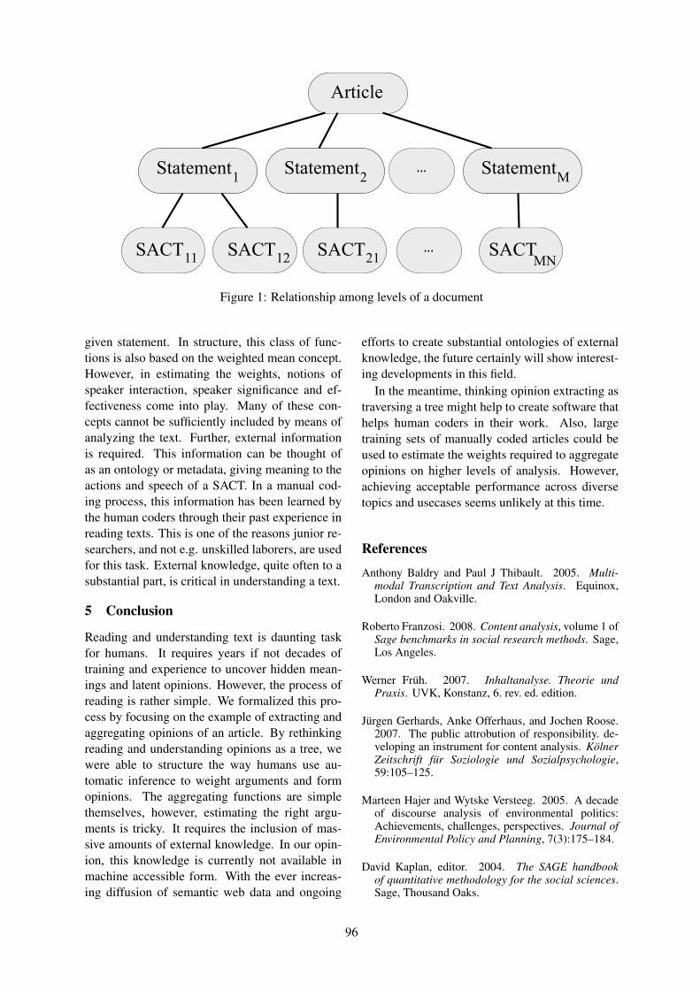
Article

Statement1

StatementM

Statement2

...

SACT11 SACT12 SACT21 SACTMN

...

Figure 1: Relationship among levels of a document

given statement. In structure, this class of func-tions is also based on the weighted mean concept.However, in estimating the weights, notions ofspeaker interaction, speaker significance and ef-fectiveness come into play. Many of these con-cepts cannot be sufficiently included by means ofanalyzing the text. Further, external informationis required. This information can be thought ofas an ontology or metadata, giving meaning to theactions and speech of a SACT. In a manual cod-ing process, this information has been learned bythe human coders through their past experience inreading texts. This is one of the reasons junior re-searchers, and not e.g. unskilled laborers, are usedfor this task. External knowledge, quite often to asubstantial part, is critical in understanding a text.

5 Conclusion

Reading and understanding text is daunting taskfor humans. It requires years if not decades oftraining and experience to uncover hidden mean-ings and latent opinions. However, the process ofreading is rather simple. We formalized this pro-cess by focusing on the example of extracting andaggregating opinions of an article. By rethinkingreading and understanding opinions as a tree, wewere able to structure the way humans use au-tomatic inference to weight arguments and formopinions. The aggregating functions are simplethemselves, however, estimating the right argu-ments is tricky. It requires the inclusion of mas-sive amounts of external knowledge. In our opin-ion, this knowledge is currently not available inmachine accessible form. With the ever increas-ing diffusion of semantic web data and ongoing

efforts to create substantial ontologies of externalknowledge, the future certainly will show interest-ing developments in this field.

In the meantime, thinking opinion extracting astraversing a tree might help to create software thathelps human coders in their work. Also, largetraining sets of manually coded articles could beused to estimate the weights required to aggregateopinions on higher levels of analysis. However,achieving acceptable performance across diversetopics and usecases seems unlikely at this time.

References

Anthony Baldry and Paul J Thibault. 2005. Multi-modal Transcription and Text Analysis. Equinox,London and Oakville.

Roberto Franzosi. 2008. Content analysis, volume 1 ofSage benchmarks in social research methods. Sage,Los Angeles.

Werner Fruh. 2007. Inhaltanalyse. Theorie undPraxis. UVK, Konstanz, 6. rev. ed. edition.

Jurgen Gerhards, Anke Offerhaus, and Jochen Roose.2007. The public attrobution of responsibility. de-veloping an instrument for content analysis. KolnerZeitschrift fur Soziologie und Sozialpsychologie,59:105–125.

Marteen Hajer and Wytske Versteeg. 2005. A decadeof discourse analysis of environmental politics:Achievements, challenges, perspectives. Journal ofEnvironmental Policy and Planning, 7(3):175–184.

David Kaplan, editor. 2004. The SAGE handbookof quantitative methodology for the social sciences.Sage, Thousand Oaks.

96

Klaus Krippendorf. 2004. Content analysis. An in-troduction to its methodology. Sage, London, 2. ededition.

Sharon M Livesey. 2001. Eco-identity as discursivestruggle: Royal dutch/shell, brent spar and nigeria.Journal of Business Communication, 38(1):58–91.

Denis McQuail. 2005. McQuail’s Mass Communica-tion Theory. Sage, London, 5. ed edition.

Klaus Merten. 1995. Inhaltsanalyse. Einfuhrungin Theorie, Methode und Praxis. Westdt. Verlag,Opladen.

Kimberly A Neuendorf. 2007. The content analysisguidebook. Sage, Thousand Oaks.

Daniel Riffe, Stephen Lacy, and Frederick Fico. 1998.Analyzing media messages: using quantitative con-tent analysis in research. Erlbaum, Mahwah.

C W Roberts. 2001. Content analysis. In Smelser andBaltes (Smelser and Baltes, 2001).

Patrick Rossler. 2005. Inhaltsanalyse. UVK, Kon-stanz.

Neil J Smelser and Paul B Baltes, editors. 2001. Inter-national Encyclopedia of the Social & BehavioralScience. Elsevier, Amsterdam.

Niranjala Weerakkody. 2009. Research Methodsfor Media and Communication. Oxford UniversityPress, Oxford.

97

Proceedings of the 2010 Workshop on Graph-based Methods for Natural Language Processing, ACL 2010, pages 98–102,Uppsala, Sweden, 16 July 2010. c©2010 Association for Computational Linguistics

Eliminating Redundancy by Spectral Relaxation for Multi-DocumentSummarization

Fumiyo Fukumoto Akina Sakai Yoshimi SuzukiInterdisciplinary Graduate School of Medicine and Engineering

University of Yamanashi{fukumoto, t05kg014, ysuzuki}@yamanashi.ac.jp

Abstract

This paper focuses on redundancy, over-lapping information in multi-documents,and presents a method for detectingsalient, key sentences from documentsthat discuss the same event. To elimi-nate redundancy, we used spectral clus-tering and classified each sentence intogroups, each of which consists of seman-tically related sentences. Then, we ap-plied link analysis, the Markov RandomWalk (MRW) Model to deciding the im-portance of a sentence within documents.The method was tested on the NTCIRevaluation data, and the result shows theeffectiveness of the method.

1 Introduction

With the exponential growth of information on theInternet, it is becoming increasingly difficult for auser to read and understand all the materials froma series of large-scale document streams that is po-tentially of interest. Multi-document summariza-tion is an issue to attack the problem. It differsfrom single document summarization in that it isimportant to identify differences and similaritiesacross documents. Graph-based ranking methods,such as PageRank (Page et al., 1998) and HITS(Kleinberg, 1999) have recently applied and beensuccessfully used for multi-document summariza-tion (Erkan and Radev, 2004; Mihalcea and Tarau,2005). Given a set of documents, the model con-structs graph consisting vertices and edges wherevertices are sentences and edges reflect the rela-tionships between sentences. The model then ap-plies a graph-based ranking method to obtain therank scores for the sentences. Finally, the sen-tences with large rank scores are chosen into thesummary. However, when they are strung to-gether, the resulting summary still contains much

overlapping information. Because all the sen-tences are ranked based on a sentence as unit ofinformation. Therefore, for example, semanti-cally related two sentences with “high recommen-dation” are ranked with high score, and thus areregarded as a summary sentence. To attack theproblem, Wan et al. proposed two models, i.e., theCluster-based conditional Markov Random Walkmodel and the Cluster-based HITS model, bothmake use of the theme clusters in the document set(Wan and Yang, 2008). Their model first groupsdocuments into theme clusters by using a simpleclustering method, k-means. Next, the model con-structs a directed or undirected graph to reflect therelationships between sentences and clusters byusing link analysis. They reported that the resultson the DUC2001 and DUC2002 datasets showedthe effectiveness of their models. However, oneof the problems using multivariate clustering suchas k-means is that it is something of a black artwhen applied to high-dimensional data. The avail-able techniques for searching this large space donot offer guarantees of global optimality, thus theresulting summary still contains much overlappinginformation, especially for a large amount of doc-uments.

This paper focuses extractive summarization,and present a method for detecting key sentencesfrom documents that discuss the same event. LikeWan et al.’s approach, we applied link analysis,the Markov Random Walk (MRW) model (Bre-maud, 1999) to a graph consisting sentences andclusters. To attack the problem dealing with thehigh dimensional spaces, we applied spectral clus-tering technique (Ng et al., 2002) to the sentencesfrom a document set. Spectral clustering is a trans-formation of the original sentences into a set of or-thogonal eigenvectors. We worked in the space de-fined by the first few eigenvectors, using standardclustering techniques in the transformed space.

98

2 Spectral Clustering

Similar to other clustering algorithms, the spec-tral clustering takes as input a matrix formed froma pairwise similarity function over a set of datapoints. Given a set of points S = {s1, · · · , sn}in a high dimensional space, the algorithm is asfollows:

1. Form a distance matrix D ∈ R2. We usedcosine similarity as a distance measure.

2. D is transformed to an affinity matrix Aij .

Aij =

{exp(−D2

ij

σ2 ), if i �= j0, otherwise.

σ2 is a parameter and controls the rate atwhich affinity drops off with distance.

3. The matrix L = D−1/2AD−1/2 is created. Dis a diagonal matrix whose (i,i) element is thesum of A’s i-th row.

4. The eigenvectors and eigenvalues of L arecomputed, and a new matrix is created fromthe vectors associated with the number of llargest eigenvalues.

5. Each item now has a vector of l coordinatesin the transformed space. These vectors arenormalized to unit length.

6. K-means is applied to S in the l-dimensionalspace.

3 Cluster-based Link Analysis

The link analysis we used is an approach presentedby Wan et. al (Wan and Yang, 2008). The modelcalled “Cluster-based Conditional Markov Ran-dom Walk Model” incorporates the cluster-levelinformation into the process of sentence rank-ing. The model is summarized as follows: Letπ(clus(si)) ∈ [0, 1] be the importance of clus-ter clus(si) in the whole document set D. Letalso ω(si, clus(si)) ∈ [0, 1] denote the strength ofthe correlation between sentence si and its clusterclus(si). clus(si) refers to the cluster containingsentence si. The transition probability from si tosj is defined by formula (1).

p(i→j|clus(si), clus(sj))

=

8>>><>>>:

f(i→j|clus(si), clus(sj))|S|Xk=1

f(i→k|clus(si), clus(sk))

, if Σf �= 0

0 , otherwise.

(1)

f(i → j | clus(si), clus(sj)) in formula (1) refersto the weight between two sentences si and sj ,conditioned on the two clusters containing the twosentences, and defined by formula (2).

f(i→j|clus(si), clus(sj))

= f(i→j)·{λ·π(clus(si))·ω(clus(si))

+(1− λ)·π(clus(sj))·ω(clus(sj))} (2)

λ ∈ [0, 1] in formula (2) is the combinationweight controlling the relative contributions fromthe source cluster and the destination cluster.π(clus(si)) denotes the value indicating the im-portance of the cluster clus(si) in the documentset D. Similarly, ω(si, clus(si)) refers to the sim-ilarity value between the sentence si and its clusterclus(si). These values are obtained by using thecosine similarity. The new row-normalized matrixM is defined by formula (3).

Mij = p(i → j | clus(si), clus(sj)) (3)

The saliency scores for the sentences are com-puted based on formula (3) by using the iterativeform in formula (4).

Score(si) = μX

allj �=i

Score(sj) · Mji +(1 − μ)

| S | (4)

μ in formula (4) is the damping factor, which weset to 0.85. The above process can be consideredas a Markov chain by taking the sentences as thestates and the final transition matrix is given byformula (5), and each score of the sentences is ob-tained by the principle eigenvector of the new tran-sition matrix A.

A = μMT +(1− μ)

| V | �e�eT (5)

�e in formula (5) is a column vector with all ele-ments equal to 1. We selected a certain numberof sentences according to rank score into the sum-mary.

99

4 Experiments

We had an experiment by using the NTCIR-31

SUMM to evaluate our approach. NTCIR-3 hastwo tasks, single, and multi-document summariza-tion. The data is collected from two years(1998-1999) Mainichi Japanese Newspaper articles. Weused multi-document summarization task. Thereare two types of gold standard data provided tohuman judges, FBFREE DryRun and FormalRun,each of which consists of 30 topics. There are twotypes of correct summary according to the charac-ter length, i.e., “long” and “short”. All documentswere tagged by a morphological analysis, ChaSen(Matsumoto et al., 1997) and noun words are ex-tracted.

We used FormalRun consisting of 30 topics as atest data. Similarly, we randomly chose 10 topicsfrom the FBFREE DryRun data to tuning a param-eter σ in Spectral Clustering, and the number of lin the l-dimensional space obtained by the Spec-tral Clustering. σ is searched in steps of 0.01 from1.0 to 5.0. l in the l-dimensional space is searchedin steps 10% from 0 to 80% against the total num-ber of words in the training data. The size that op-timized the average F-score of 10 topics was cho-sen. Here, F-score is the standard measure usedin the clustering algorithm, and it combines recalland precision with an equal weight. Precision is aratio of the number of correct pair of sentences ob-tained by the k-means divided by the total numberof pairs obtained by the k-means. Recall indicatesa ratio of the number of correct pair of sentencesobtained by the k-means divided by the total num-ber of correct pairs. As a result, σ and l are set to4.5 and 80%, respectively.

It is difficult to predict the actual cluster numberk in a given input sentences to produce optimalresults. The usual drawback in many clusteringalgorithms is that they cannot give a valid criterionfor measuring class structure. Therefore, similarto Wan et. al’s method (Wan and Yang, 2008), wetypically set the number of k of expected clustersas

√N where N is the number of all sentences

in the document set. We used these values of theparameters and evaluated by using test data.

We used two evaluation measures. One is co-sine similarity between the generated summary bythe system and the human generated summary.Another is ROUGE score used in DUC (Liu andHovy, 2003).

1http://research.nii.ac.jp/ntcir/

ROUGE =

Xs∈Cand

Xngram∈s

Countmatch(ngram)

Xs∈Cand

Xngram∈s

Count(ngram)(6)

We used a word instead of n-gram sequence informula (6). The results are shown in Table 1. “#of doc” and “# of sent” refer to the average numberof documents and sentences, respectively. “# ofsum” denotes to the average number of summarysentences provided by NTCIR3 SUMM. “cos” and“ROUGE” refer to the results evaluated by usingcosine, and ROUGE score, respectively. “MRW”indicates the results obtained by directly applyingMRW model to the input sentences.

We can see from Table 1 that our approach(Spectral) outperforms the baselines, “MRW”and “k-means”, regardless of the types of sum-mary (long/short) and evaluation measures (co-sine/ROUGE). The results obtained by three ap-proaches show that “short” was better than “long”.This indicates that the rank score of correct sen-tences within the candidate sentences obtainedby the MRW model works well. Comparingthe results evaluated by “ROUGE” were worsethan those of “cos” at any approaches. One rea-son is that the difference of summarization tech-nique, i.e., our work is extractive summarization,while the gold standard data provided by NTCIR-3 SUMM is the abstracts written by human pro-fessionals. As a result, a large number of wordsin a candidate summary are extracted by our ap-proaches. For future work, it is necessary to ex-tend our method to involve paraphrasing for ex-tracted key sentences to reduce the gap betweenautomatically generated summaries and human-written abstracts (Barzilay et al., 1993; Careniniand Cheung, 2008).

It is interesting to note how our approach affectsfor the number of sentences as an input. Figure1 illustrates the results of summary “long” withevaluated ROUGE score. We can see from Figure1 that our approach is more robust than k-meansand the MRW model, even for a large number ofinput data. We have seen the same observationsfrom other three results, i.e., the results of shortand long with evaluated cos and short with evalu-ated ROUGE.

We recall that the cluster number k is set to thesquare root of the sentence number. We tested dif-ferent number of k to see how the cluster number

100

Table 1: Results against 30 topics

# of doc # of sent # of sum cos ROUGEMRW k-means Spectral MRW k-means Spectral

Short 7.5 83.0 11.9 0.431 0.575 0.632 0.330 0.334 0.360Long 20.4 0.371 0.408 0.477 0.180 0.186 0.209

0.05

0.1

0.15

0.2

0.25

0.3

0.35

0.4

0 50 100 150 200 250 300 350

RO

UG

E

# of sentences

k-meansSpectral

MRW

Figure 1: Long with ROUGE vs. # of sentences

affects the summarization performance. In the ex-periment, we set k = r∗ | N | where r is a pa-rameter ranged from 0 to 1 (Wan and Yang, 2008).Because of space is limited, we report only the re-sult with summary “long” and ROUGE score. Theresult is shown in Figure 2.

Overall the results obtained by our approachand k-means outperformed the results obtainedby directly applying MRW model, while the re-sults by k-means was worse than the results byMRW model when the ratio of the number of sen-tences was larger than 0.8. This shows that cluster-based summarization is effective reduce redun-dancy, overlapping information. Figure 2 alsoshows that our approach always outperforms, re-gardless of how many number of sentences wereused. This indicates that the MRW model withspectral clustering is more robust than that withthe baseline, k-means, with respect to the differ-ent number of clusters.

5 Conclusion

We have developed an approach to detect salientsentences from documents that discuss the same

0.175

0.18

0.185

0.19

0.195

0.2

0.205

0.21

0.1 0.2 0.3 0.4 0.5 0.6 0.7 0.8 0.9

Avg

. R

OU

GE

ratio of the # of k

MRWk-meansSpectral

Figure 2: Long with ROUGE score measure vs. #of k

event. The results showed the effectiveness of themethod. Future work will include: (i) compar-ing other approaches that uses link analysis to re-duce redundancy, such as (Zhu et al., 2007), (ii)applying the method to the DUC evaluation datafor quantitative evaluation, and (iii) extending themethod to classify sentences into more than oneclasses by using soft-clustering techniques such asEM (Dempster et al., 1977) and fuzzy c-means al-gorithms (Zhang and Wang, 2007).

References

R. Barzilay, K. R. McKeown, and M. Elhadad.1993. Information Fusion in the Context of Multi-document Summarization. In Proc. of the 37th An-nual Meeting of the Association for ComputationalLinguistics, pages 550–557.

P. Bremaud. 1999. Markov Chains: Gibbs Fields,Monte Carlo Simulation, and Queues. Springer-Verlag.

G. Carenini and J. C. K. Cheung. 2008. Extractivevs. NLG-based Abstractive Summarization of Eval-uative Text: The Effect of Corpus Controversiality.

101

In Proc. of the 5th International Natural LanguageGeneration Conference, pages 33–41.

A. P. Dempster, N. M. Laird, and D. B. Rubin. 1977.Maximum Likelihood from Incomplete Data Via theEM Algorithm. Royal Statistical Society, 39(B):1–38.

G. Erkan and D. Radev. 2004. LexPageRank: Prestigein Multi-document Text Summarization. In Proc. ofthe 2004 Conference on Empirical Methods in Nat-ural Language Processing, pages 365–371.

J. M. Kleinberg. 1999. Authoritative Sources in a Hy-perlinked Environment. ACM, 46(5):604–632.

C-Y. Liu and E. H. Hovy. 2003. Automatic Evalu-ation of Summaries Using N-gram Co-occurrenceStatistics. In Proc. of Human Language Technolo-gies: The Annual Conference of the North AmericanChapter of the Association for Computational Lin-guistics, pages 71–78.

Y. Matsumoto, A. Kitauchi, T. Yamashita, Y. Haruno,O. Imaichi, and T. Imamura. 1997. Japanese Mor-phological Analysis System Chasen Mannual.

R. Mihalcea and P. Tarau. 2005. Language Indepen-dent Extractive Summarization. In In Proc. of the43nd Annual Meeting of the Association for Compu-tational Linguistics, pages 49–52.

A. Y. Ng, M. I. Jordan, and Y. Weiss. 2002. On Spec-tral Clustering: Analysis and an Algorithm, vol-ume 14. MIT Press.

L. Page, S. Brin, R. Motwani, and T. Winograd. 1998.The Pagerank Citation Ranking: Bringing Order tothe Web. In Technical report, Stanford Digital Li-braries.

X. Wan and J. Yang. 2008. Multi-document Sum-marization Using Cluster-based Link Analysis. InProc. of the 31st Annual International ACM SIGIRConference on Research and Development in Infor-mation Retrieval, pages 299–306.

Z. Zhang and R. Wang. 2007. Identification ofOverlapping Community Structure in Complex Net-works using Fuzzy C-means Clustering. PHYSICA,A(374):483–490.

X. Zhu, A. Goldberg, J. V. Gael, and D. Andrzejew-ski. 2007. Improving Diversity in Ranking usingAbsorbing Random Walks. In In Human Languagetechnologies: The Annual Conference of the NorthAmerican Chapter of the Association for Computa-tional Linguistics, pages 97–104.

102

Proceedings of the 2010 Workshop on Graph-based Methods for Natural Language Processing, ACL 2010, pages 103–107,Uppsala, Sweden, 16 July 2010. c©2010 Association for Computational Linguistics

Computing Word Senses by Semantic Mirroring and Spectral GraphPartitioning

Martin FagerlundLinkoping UniversityLinkoping, Sweden

marfa229@student.liu.se

Lars EldenLinkoping UniversityLinkoping, Sweden

lars.elden@liu.se

Magnus MerkelLinkoping UniversityLinkoping, Sweden

magnus.merkel@liu.se

Lars AhrenbergLinkoping UniversityLinkoping, Sweden

lars.ahrenberg@liu.se

Abstract

Using the technique of ”semantic mirror-ing” a graph is obtained that representswords and their translations from a paral-lel corpus or a bilingual lexicon. The con-nectedness of the graph holds informationabout the different meanings of words thatoccur in the translations. Spectral graphtheory is used to partition the graph, whichleads to a grouping of the words accordingto different senses. We also report resultsfrom an evaluation using a small sample ofseed words from a lexicon of Swedish andEnglish adjectives.

1 Introduction

A great deal of linguistic knowledge is encodedimplicitly in bilingual resources such as par-allel texts and bilingual dictionaries. Dyvik(1998, 2005) has provided a knowledge discov-ery method based on the semantic relationship be-tween words in a source language and words ina target language, as manifested in parallel texts.His method is called Semantic mirroring and theapproach utilizes the way that different languagesencode lexical meaning by mirroring source wordsand target words back and forth, in order to es-tablish semantic relations like synonymy and hy-ponymy. Work in this area is strongly related towork within Word Sense Disambiguation (WSD)and the observation that translations are a goodsource for detecting such distinctions (Resnik &Yarowsky 1999, Ide 2000, Diab & Resnik 2002).A word that has multiple meanings in one lan-guage is likely to have different translations inother languages. This means that translationsserve as sense indicators for a particular source

word, and make it possible to divide a given wordinto different senses.

In this paper we propose a new graph-based ap-proach to the analysis of semantic mirrors. Theobjective is to find a viable way to discover syn-onyms and group them into different senses. Themethod has been applied to a bilingual dictionaryof English and Swedish adjectives.

2 Preparations

2.1 The Translation MatrixIn these experiments we have worked with aEnglish-Swedish lexicon consisting of 14850 En-glish adjectives, and their corresponding Swedishtranslations. Out of the lexicon was created atranslation matrix B, and two lists with all thewords, one for English and one for Swedish. Bis defined as

B(i, j) =

{1, if i ∼ j,0, otherwise.

The relation i ∼ j means that word i translatesto word j.

2.2 TranslationTranslation is performed as follows. From theword i to be translated, we create a vector ei, witha one in position i, and zeros everywhere else.Then perform the matrix multiplication Bei if itis a Swedish word to be translated, or BT ei if it isan English word to be translated. ei has the samelength as the list in which the word i can be found.

3 Semantic Mirroring

We start with an English word, called eng11. Welook up its Swedish translations. Then we look up

1Short for english1. We will use swe for Swedish words.

103

the English translations of each of those Swedishwords. We have now performed one ”mirror-operation”. In mathematical notation:

f = BBT eeng1.

The non-zero elements in the vector f representEnglish words that are semantically related toeng1. Dyvik (1998) calls the set of words that weget after two translations the inverse t-image. Butthere is one problem. The original word should notbe here. Therefore, in the last translation, we mod-ify the matrix B, by replacing the row in B corre-sponding to eng1, with an all-zero row. Call thisnew modified matrix Bmod1. So instead of the ma-trix multiplication performed above, we start overwith the following one:

Bmod1BT eeng1. (1)

To make it clearer from a linguistic perspective,consider the following figure2.

eng2

swe1

33ffffffffff eng3

eng1++XXXXXXXXXX //

33ffffffffffswe2

33ffffffffff

++XXXXXXXXXX eng1

swe3 //

++XXXXXXXXXX eng4

eng5

The words to the right in the picture above(eng2,...,eng5) are the words we want to divideinto senses. To do this, we need some kind ofrelation between the words. Therefore we con-tinue to translate, and perform a second ”mirroroperation”. To keep track of what each word inthe inverse t-image translates to, we must firstmake a small modification. We have so far donethe operation (1), which gave us a vector, call ite ∈ R14850×1. The vector e consists of nonzero in-tegers in the positions corresponding to the wordsin the invers t-image, and zeros everywhere else.We make a new matrix E, with the same numberof rows as e, and the same number of columns asthere are nonzeros in e. Now go through every el-ement in e, and when finding a nonzero elementin row i, and if it is the j:th nonzero element, thenput a one in position (i, j) in E. The procedure isillustrated in (2).

2The arrows indicate translation.

102103

−→

1 0 0 00 0 0 00 1 0 00 0 1 00 0 0 00 0 0 1

(2)

When doing our second ”mirror operation”, we donot want to translate through the Swedish wordsswe1,...,swe3. We once again modify the matrixB, this time replacing the columns of B corre-sponding to the Swedish words swe1,...,swe3, withzeros. Call this second modified matrix Bmod2.With the matrix E from (2), we now get:

Bmod2BTmod2E (3)

We illustrate the operation (3):

swe4 //))SSSS eng6

eng255kkkk // swe5 //

))SSSS eng2

swe155kkkkeng3

55kkkkswe1 eng3

eng1))SSSS //55kkkkswe2

55kkkk

))SSSS eng1 swe2 eng1

swe3 //))SSSS eng4

))SSSS swe3 eng4

eng5 //))SSSS swe6

55kkkk //))SSSS eng5

swe755kkkk // eng7

Now we have got the desired relation betweeneng2,...eng5. In (3) we keep only the rows corre-sponding to eng2,...eng5, and get a symmetric ma-trix A, which can be considered as the adjacencymatrix of a graph. The adjacency matrix and thegraph of our example are illustrated below.

A =

2 1 0 01 1 0 00 0 1 10 0 1 2

(4)

eng2

eng3

eng4

eng5

Figure 1: The graph to the matrix in (4).

The adjacency matrix should be interpreted in thefollowing way. The rows and the columns corre-spond to the words in the inverse t-image. Follow-ing our example, eng2 corresponds to row 1 and

104

column 1, eng3 corresponds to row 2 and column2, and so on. The elements on position (i, i) inA are the vertex weights. The vertex weight as-sociated with a word, describes how many transla-tions that word has in the other language, e.g. eng2translates to swe4 and swe5 that is translated backto eng2. So the vertex weight for eng2 is 2, as alsocan be seen in position (1, 1) in (4). A high vertexweight tells us that the word has a high number oftranslations, and therefore probably a wide mean-ing.

The elements in the adjacency matrix on posi-tion (i, j), i = j are the edge weights. Theseweights are associated with two words, and de-scribe how many words in the other language thatboth word i and j are translated to. E.g. eng5and eng4 are both translated to swe6, and it fol-lows that the weight, w(eng4,eng5) = 1. If we in-stead would take eng5 and eng7, we see that theyboth translate to swe6 and swe7, so the weight be-tween those words, w(eng5,eng7) = 2. (But this isnot shown in the adjacency matrix, since eng7 isnot a word in the inverse t-image). A high edgeweight between two words tells us that they sharea high number of translations, and therefore prob-ably have the same meanings.

4 Graph Partitioning

The example illustrated in Figure 1 gave as a re-sult two graphs that are not connected. Dyvik ar-gues that in such a case the graphs represent twogroups of words of different senses. In a largerand more realistic example one is likely to obtaina graph that is connected, but which can be parti-tioned into two subgraphs without breaking morethan a small number of edges. Then it is reason-able to ask whether such a partitioning has a sim-ilar effect in that it represents a partitioning of thewords into different senses.

We describe the mathematical procedure of par-titioning a graph into subgraphs, using spectralgraph theory (Chung, 1997). First, define the de-gree d(i) of a vertex i to be

d(i) =∑

j

A(i, j).

Let D be the diagonal matrix defined by

D(i, j) =

{d(i), if i = j,0, otherwise.

The Laplacian L is defined as

L = D −A.

We define the normalised Laplacian L to be

L = D− 12 LD− 1

2 .

Now calculate the eigenvalues λ0, . . . , λn−1, andthe eigenvectors of L. The smallest eigen-value, λ0, is always equal to zero, as shown byChung (1997). The multiplicity of zero amongthe eigenvalues is equal to the number of con-nected components in the graph, as shown bySpielman (2009). We will look at the eigenvectorbelonging to the second smallest eigenvalue, λ1.This eigenpair is often referred to as the Fiedlervalue and the Fiedler vector. The entries in theFiedler vector corresponds to the vertices in thegraph. (We will assume that there is only onecomponent in the graph. If not, chose the com-ponent with the largest number of vertices). Sortthe Fiedler vector, and thus sorting the vertices inthe graph. Then make n− 1 cuts along the Fiedlervector, dividing the elements of the vector into twosets, and for each cut compute the conductance,ϕ(S), defined as

ϕ(S) = d(V )|∂(S, S) |d(S)d(S)

, (5)

where d(S) =∑

i∈S d(i). | ∂(S, S) | is the totalweight of the edges with one end in S and one endin S, and V = S + S is the set of all vertices inthe graph. Another measure used is the sparsity,sp(S), defined as

sp(S) =|∂(S, S) |

min(d(S), d(S))(6)

For details, see (Spielman, 2009). Choose the cutwith the smallest conductance, and in the graph,delete the edges with one end in S and the otherend in S. The procedure is then carried out untilthe conductance, ϕ(S), reaches a tolerance. Thetolerance is decided by human evaluators, per-forming experiments on test data.

5 Example

We start with the word slithery, and after the mir-roring operation (3) we get three groups of wordsin the inverse t-image, shown in Table 1. Aftertwo partitionings of the graph to slithery, using themethod described in section 4, we get five sensegroups, shown in Table 2.

105

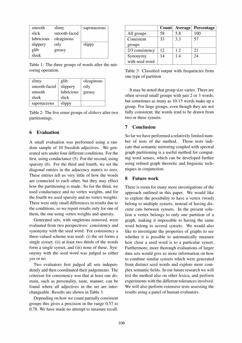
smooth slimy saponaceousslick smooth-facedlubricious oleaginousslippery oily slippyglib greasysleek

Table 1: The three groups of words after the mir-roring operation.

slimy glib oleaginoussmooth-faced slippery oilysmooth lubricious greasysleek slicksaponaceous slippy

Table 2: The five sense groups of slithery after twopartitionings.

6 Evaluation

A small evaluation was performed using a ran-dom sample of 10 Swedish adjectives. We gen-erated sets under four different conditions. For thefirst, using conductance (5). For the second, usingsparsity (6). For the third and fourth, we set thediagonal entries in the adjacency matrix to zero.These entries tell us very little of how the wordsare connected to each other, but they may effecthow the partitioning is made. So for the third, weused conductance and no vertex weights, and forthe fourth we used sparsity and no vertex weights.There were only small differences in results due tothe conditions, so we report results only for one ofthem, the one using vertex weights and sparsity.

Generated sets, with singletons removed, wereevaluated from two perspectives: consistency andsynonymy with the seed word. For consistency athree-valued scheme was used: (i) the set forms asingle synset, (ii) at least two thirds of the wordsform a single synset, and (iii) none of these. Syn-onymy with the seed word was judged as eitheryes or no.

Two evaluators first judged all sets indepen-dently and then coordinated their judgements. Thecriterion for consistency was that at least one do-main, such as personality, taste, manner, can befound where all adjectives in the set are inter-changeable. Results are shown in Table 3.

Depending on how we count partially consistentgroups this gives a precision in the range 0.57 to0.78. We have made no attempt to measure recall.

Count Average PercentageAll groups 58 5.8 100Consistentgroups

33 3.3 57

2/3 consistency 12 1.2 21Synonymywith seed word

14 1.4 24

Table 3: Classified output with frequencies fromone type of partition

It may be noted that group size varies. There areoften several small groups with just 2 or 3 words,but sometimes as many as 10-15 words make up agroup. For large groups, even though they are notfully consistent, the words tend to be drawn fromtwo or three synsets.

7 Conclusion

So far we have performed a relatively limited num-ber of tests of the method. Those tests indi-cate that semantic mirroring coupled with spectralgraph partitioning is a useful method for comput-ing word senses, which can be developed furtherusing refined graph theoretic and linguistic tech-niques in conjunction.

8 Future work

There is room for many more investigations of theapproach outlined in this paper. We would liketo explore the possibility to have a vertex (word)belong to multiple synsets, instead of having dis-crete cuts between synsets. In the present solu-tion a vertex belongs to only one partition of agraph, making it impossible to having the sameword belong to several synsets. We would alsolike to investigate the properties of graphs to seewhether it is possible to automatically measurehow close a seed word is to a particular synset.Furthermore, more thorough evaluations of largerdata sets would give us more information on howto combine similar synsets which were generatedfrom distinct seed words and explore more com-plex semantic fields. In our future research we willtest the method also on other lexica, and performexperiments with the different tolerances involved.We will also perform extensive tests assessing theresults using a panel of human evaluators.

106

ReferencesDaniel A. Spielman. 2009. Spectral Graph theory.

Lecture notes.

Daniel A. Spielman, S. -H. Teng. 2006. Spectral par-titioning works: Planar graphs and finite elementmeshes. Elsevier Inc.

Diab, M. Resnik, P. 2002. An Unsupervised Methodfor Word Sense Tagging using Parallel Corpora.Proceedings of the 40th Annual Meeting of the As-sociation for Computational Linguistics. 255-262.

Fan R. K. Chung. 1997. Spectral Graph Theory.American Mathematical Society, Providence, RhodeIsland.

H. Dyvik. 1998. A Translational Basis for Semantics.In: Stig Johansson and Signe Oksefjell (eds.): Cor-pora and Crosslinguistic Research: Theory, Methodand Case Studies, pp. 51-86. Rodopi.

H. Dyvik. 2005. Translations as a Semantic Knowl-edge Source. Proceedings of the Second Baltic Con-ference on Human Language Technologies, Tallinn.

Nancy Ide. 2000. Cross-lingual sense determination:Can it work? Computers and the Humanities: Spe-cial issue on SENSEVAL, 34:223–234.

Philip Resnik , David Yarowsky. Distinguishing sys-tems and distinguishing senses: new evaluationmethods for Word Sense Disambiguation Natu-ral Language Engineering, v.5 n.2, p.113-133, June1999

107

Author Index

Ahrenberg, Lars, 103Amancio, Diego Raphael, 83Ambwani, Geetu, 60Archer, Vincent, 69

Basili, Roberto, 24Biemann, Chris, 55Boato, Giulia, 88

Castro Jorge, Maria Lucia, 74Chen, Zheng, 1Costa, Luciano da Fontoura, 83

Davis, Anthony, 60De Cao, Diego, 24

Elden, Lars, 103Enright, Jessica, 42

Fabbri, Renato, 83Fagerlund, Martin, 103Fukumoto, Fumiyo, 98

German, Daniel, 19Gomes, Paulo, 10Goncalo Oliveira, Hugo, 10Gornerup, Olof, 48

Hancock, Edwin, 47Hare, Jonathon, 88

Ji, Heng, 1

Karlgren, Jussi, 48

Lewis, Paul, 88Luciani, Matteo, 24

Merkel, Magnus, 103Mesiano, Francesco, 24Minack, Enrico, 88

Nerbonne, John, 33Nunes, Maria das Gracas Volpe, 83

Oliveira Jr., Osvaldo Novais, 83

Pardo, Thiago, 74

Rossi, Riccardo, 24

Sakai, Akina, 98Siersdorfer, Stefan, 88Siqueira, Maity, 19Suzuki, Yoshimi, 98

Tatzl, Gabriele, 93

Villavicencio, Aline, 19

Waldhauser, Christoph, 93Wieling, Martijn, 33

Zontone, Pamela, 88

109