Proc Robust Reg
56
1 PROC ROBUSTREG –Robust Regression Models April 20, 2005 Charlie Hallahan
-
Upload
ban-hong-teh -
Category
Documents
-
view
53 -
download
1
description
Robust Mean Calculation
Transcript of Proc Robust Reg

1
PROC ROBUSTREG –Robust Regression Models
April 20, 2005
Charlie Hallahan
2
PROC ROBUSTREG is experimental in SAS/ETS Version 9.*
Main purpose is to detect outliers and provide resistant (stable) results in thepresence of outliers
Addresses three types of problems: problems with outliers in the y-direction (response direction) problems with multivariate outliers in the x-space (leverage points) problems with outliers in both the y-direction and x-space
* These notes closely follow the SAS documentation for ROBUSTREG. Also, see the paper “Robust Regression and Outlier Detection with the ROBUSTREG Procedure” by Colin Chen presented at SUGI’27 in 2002 (http://www2.sas.com/proceedings/sugi27/p265-27.pdf )
Overview
3
OverviewROBUSTREG supports four methods:
1. M estimation: introduced by Huber in 1973. Simplest both computationally and theoretically. Only addresses contamination in the response direction.
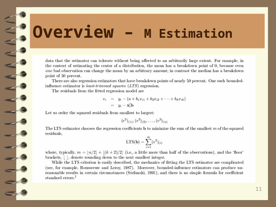
2. Least Trimmed Squares (LTS): introduced by Rouseeuw in 1984. It is aso-called high breakdown method. The breakdown value is a measure of theproportion of contamination that an estimation method can withstand andstill maintain its robustness. Uses the FAST-LST algorithm of Rouseeuw andVan Driessen (1998).
3. S estimation: introduced by Rouseeuw and Yohai in 1984. It is a high breakdown method that is more statistically efficient than LTS.
4. MM estimation: introduced by Yohai in 1987. Combines high breakdown value estimation and M estimation. It is a high breakdown method that is more
statistically efficient than S estimation
4
Overview – M Estimation
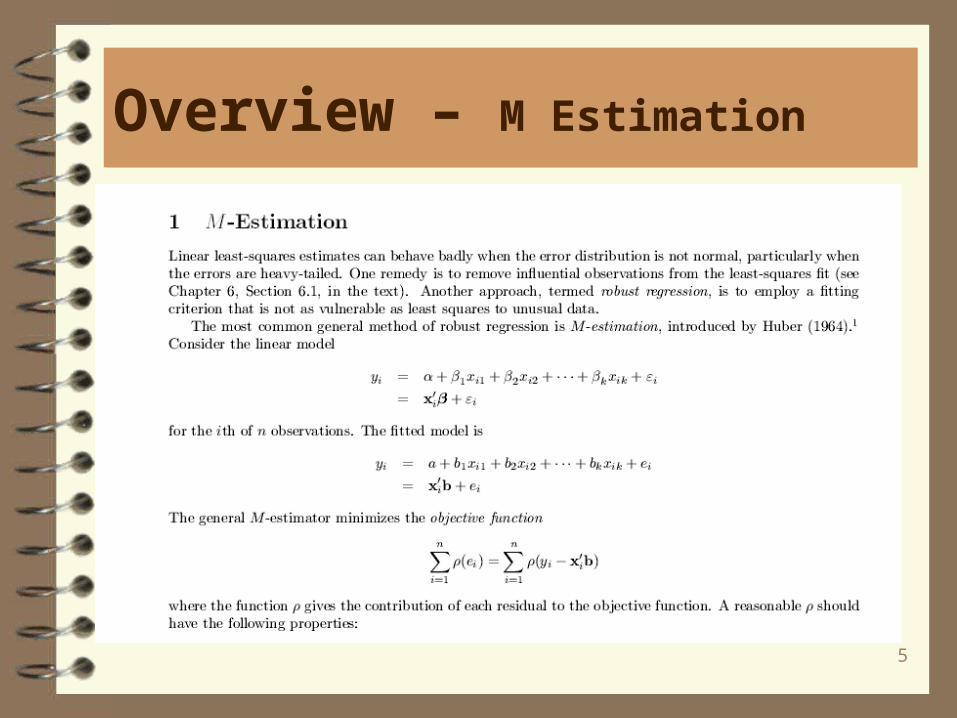
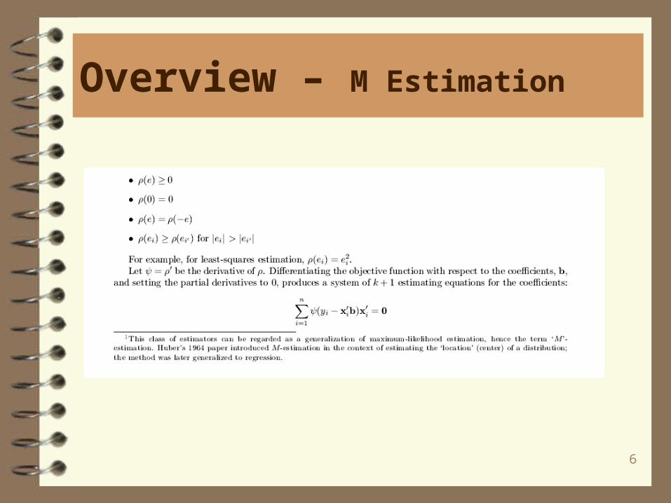
Before getting to the SAS code, it’s probably worthwhile to review what’s involvedwith the simplest robust estimator, the M estimator.
These notes follow some online documentation for the text “Applied Regression Analysis, Linear Models, and Related Methods” by John Fox.
When the error distribution is normal, least squares (LS) is the most efficient regression estimator. However, LS is very sensitive to outliers (aberrant observationsin the y-direction) at high leverage points (aberrant observations in the x-direction). Such cases result in heavy-tailed error distributions.
5
Overview – M Estimation
6
Overview – M Estimation
7
Overview – M Estimation

8
Overview – M Estimation
9
Overview – M Estimation
10
Overview – M Estimation
11
Overview – M Estimation
12
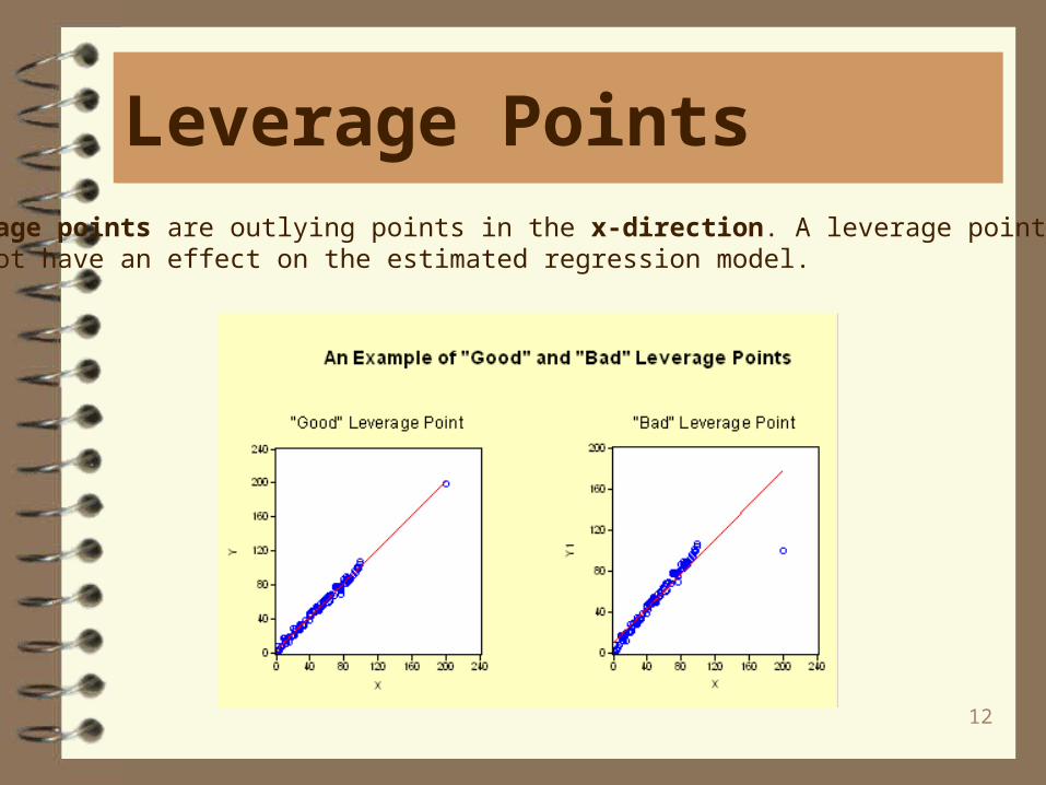
Leverage PointsLeverage points are outlying points in the x-direction. A leverage points may or may not have an effect on the estimated regression model.
13
Getting Started- M Estimation
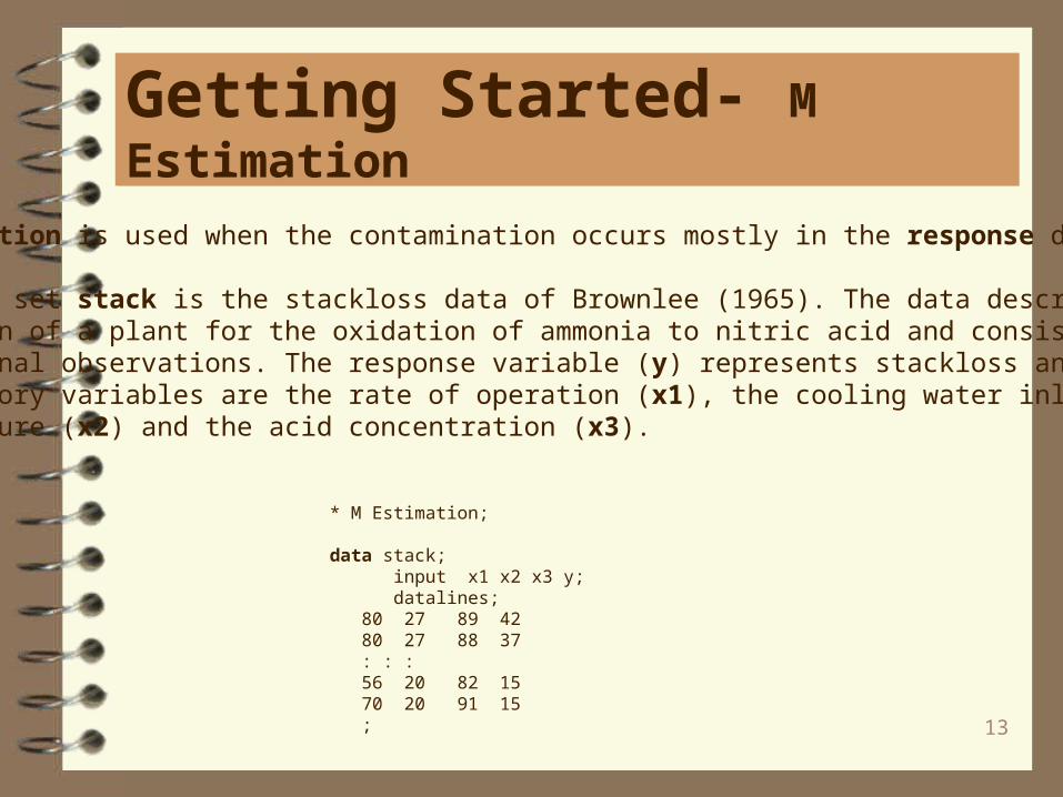
M estimation is used when the contamination occurs mostly in the response direction.
The data set stack is the stackloss data of Brownlee (1965). The data describe theoperation of a plant for the oxidation of ammonia to nitric acid and consist of 21 four-dimensional observations. The response variable (y) represents stackloss and theexplanatory variables are the rate of operation (x1), the cooling water inlet temperature (x2) and the acid concentration (x3).
* M Estimation;
data stack; input x1 x2 x3 y; datalines; 80 27 89 42 80 27 88 37 : : : 56 20 82 15 70 20 91 15 ;
14
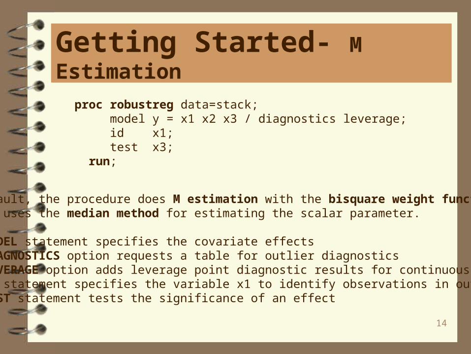
Getting Started- M Estimation
proc robustreg data=stack; model y = x1 x2 x3 / diagnostics leverage; id x1; test x3; run;
By default, the procedure does M estimation with the bisquare weight function, and it uses the median method for estimating the scalar parameter.
The MODEL statement specifies the covariate effectsThe DIAGNOSTICS option requests a table for outlier diagnosticsThe LEVERAGE option adds leverage point diagnostic results for continuous effectsThe ID statement specifies the variable x1 to identify observations in output tablesthe TEST statement tests the significance of an effect
15
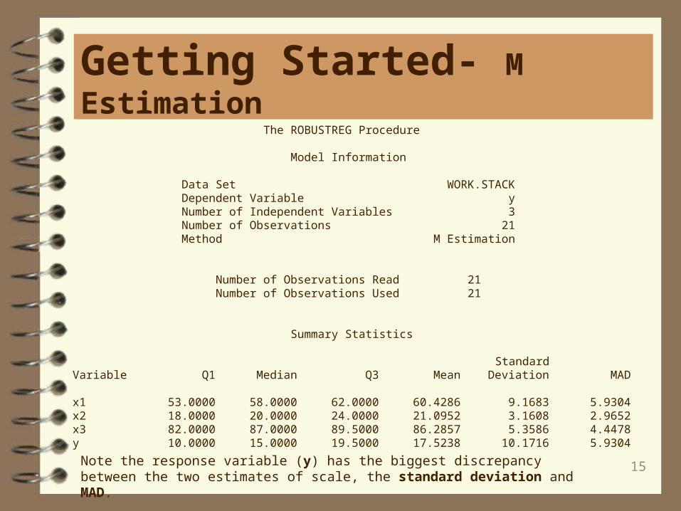
Getting Started- M Estimation The ROBUSTREG Procedure
Model Information
Data Set WORK.STACK Dependent Variable y Number of Independent Variables 3 Number of Observations 21 Method M Estimation
Number of Observations Read 21 Number of Observations Used 21
Summary Statistics
Standard Variable Q1 Median Q3 Mean Deviation MAD
x1 53.0000 58.0000 62.0000 60.4286 9.1683 5.9304 x2 18.0000 20.0000 24.0000 21.0952 3.1608 2.9652 x3 82.0000 87.0000 89.5000 86.2857 5.3586 4.4478 y 10.0000 15.0000 19.5000 17.5238 10.1716 5.9304
Note the response variable (y) has the biggest discrepancy between the two estimates of scale, the standard deviation and MAD.
16
Getting Started- M Estimation
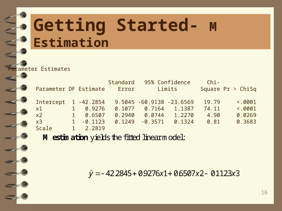
Parameter Estimates
Standard 95% Confidence Chi- Parameter DF Estimate Error Limits Square Pr > ChiSq
Intercept 1 -42.2854 9.5045 -60.9138 -23.6569 19.79 <.0001 x1 1 0.9276 0.1077 0.7164 1.1387 74.11 <.0001 x2 1 0.6507 0.2940 0.0744 1.2270 4.90 0.0269 x3 1 -0.1123 0.1249 -0.3571 0.1324 0.81 0.3683 Scale 1 2.2819
M estimation yields the fitted linear model:
. . . .y x x x 42 2845 0 9276 1 0 6507 2 01123 3
17
Getting Started- M Estimation
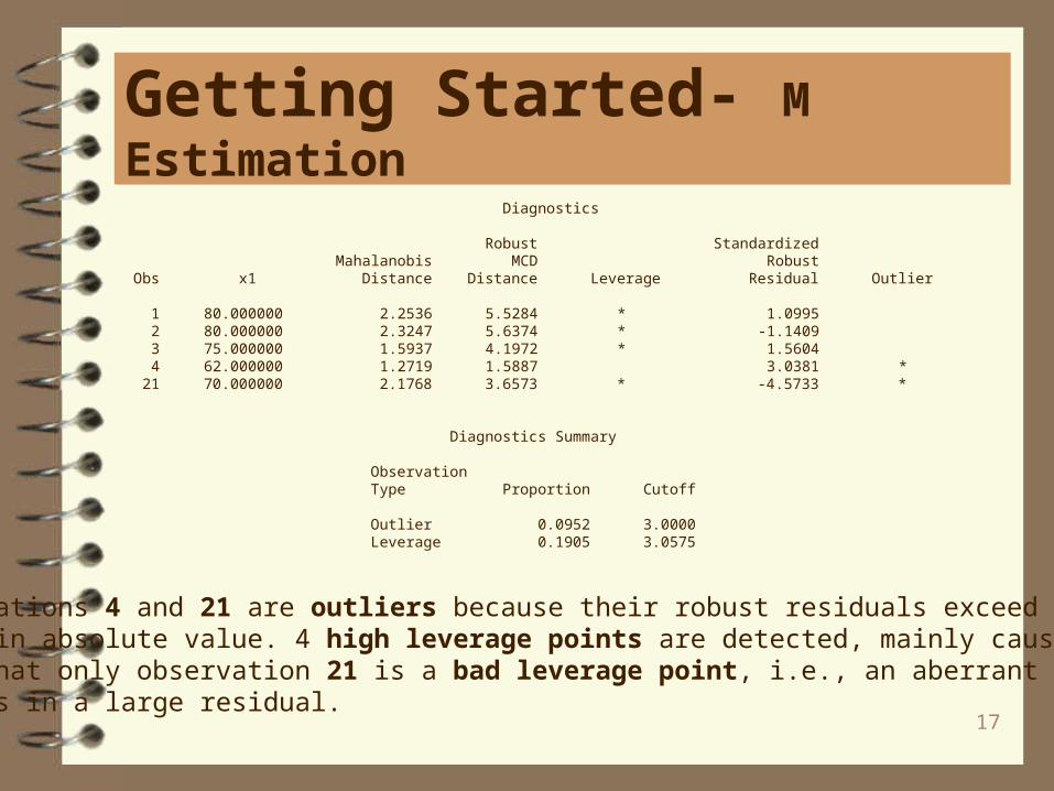
Diagnostics
Robust Standardized Mahalanobis MCD Robust Obs x1 Distance Distance Leverage Residual Outlier
1 80.000000 2.2536 5.5284 * 1.0995 2 80.000000 2.3247 5.6374 * -1.1409 3 75.000000 1.5937 4.1972 * 1.5604 4 62.000000 1.2719 1.5887 3.0381 * 21 70.000000 2.1768 3.6573 * -4.5733 *
Diagnostics Summary
Observation Type Proportion Cutoff
Outlier 0.0952 3.0000 Leverage 0.1905 3.0575
Observations 4 and 21 are outliers because their robust residuals exceed the cutoff value in absolute value. 4 high leverage points are detected, mainly caused by x1.Note that only observation 21 is a bad leverage point, i.e., an aberrant x-value thatresults in a large residual.
18
Getting Started- M Estimation
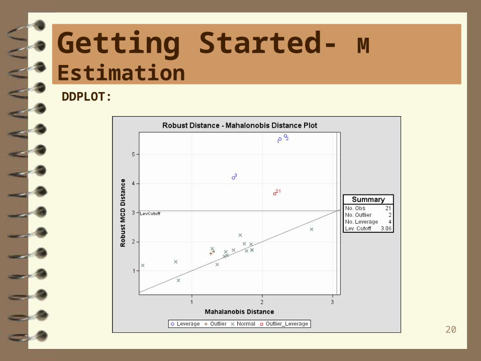
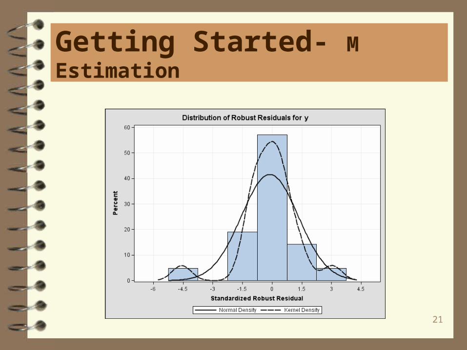
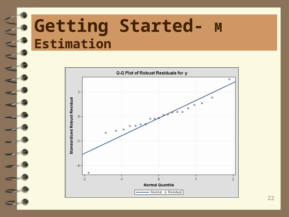
Two useful plots are the RDPLOT, robust residuals against robust distances. and theDDPLOT, robust distances against classical Mahalanobis distances. Residual plotsare also useful.
These plots are available with ODS GRAPHICS.
ods html; ods graphics on; proc robustreg data=stack plots=(rdplot ddplot reshistogram resqqplot); model y = x1 x2 x3; run; ods graphics off; ods html close;
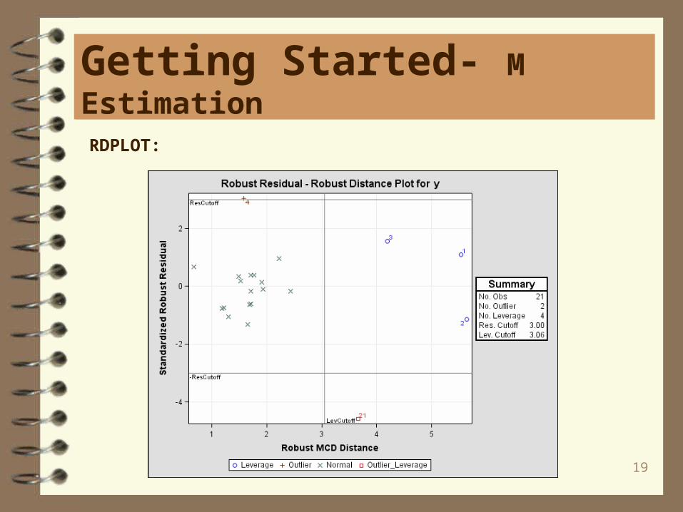
19
Getting Started- M Estimation
RDPLOT:
20
Getting Started- M Estimation
DDPLOT:
21
Getting Started- M Estimation
22
Getting Started- M Estimation

23
Getting Started- M Estimation
Goodness-of-Fit
Statistic Value
R-Square 0.6659 AICR 29.5231 BICR 36.3361 Deviance 125.7905
Robust Linear Tests*
Test
Test Chi- Test Statistic Lambda DF Square Pr > ChiSq
Rho 0.9378 0.7977 1 1.18 0.2782 Rn2 0.8092 1 0.81 0.3683
Rho is a robust version of the F-test, and Rn2 is a robust version of the Wald test.
24
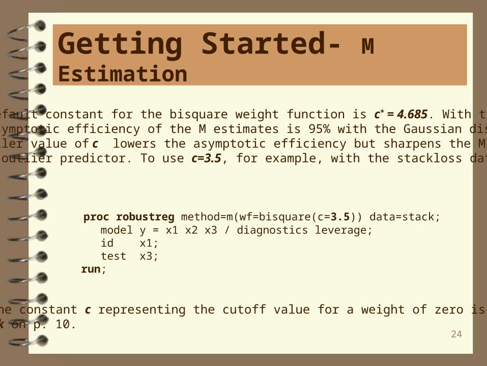
Getting Started- M Estimation
The default constant for the bisquare weight function is c* = 4.685. With this valuethe asymptotic efficiency of the M estimates is 95% with the Gaussian distribution.A smaller value of c lowers the asymptotic efficiency but sharpens the M estimatoras an outlier predictor. To use c=3.5, for example, with the stackloss data set:
proc robustreg method=m(wf=bisquare(c=3.5)) data=stack; model y = x1 x2 x3 / diagnostics leverage; id x1; test x3; run;
* The constant c representing the cutoff value for a weight of zero is called k on p. 10.
25
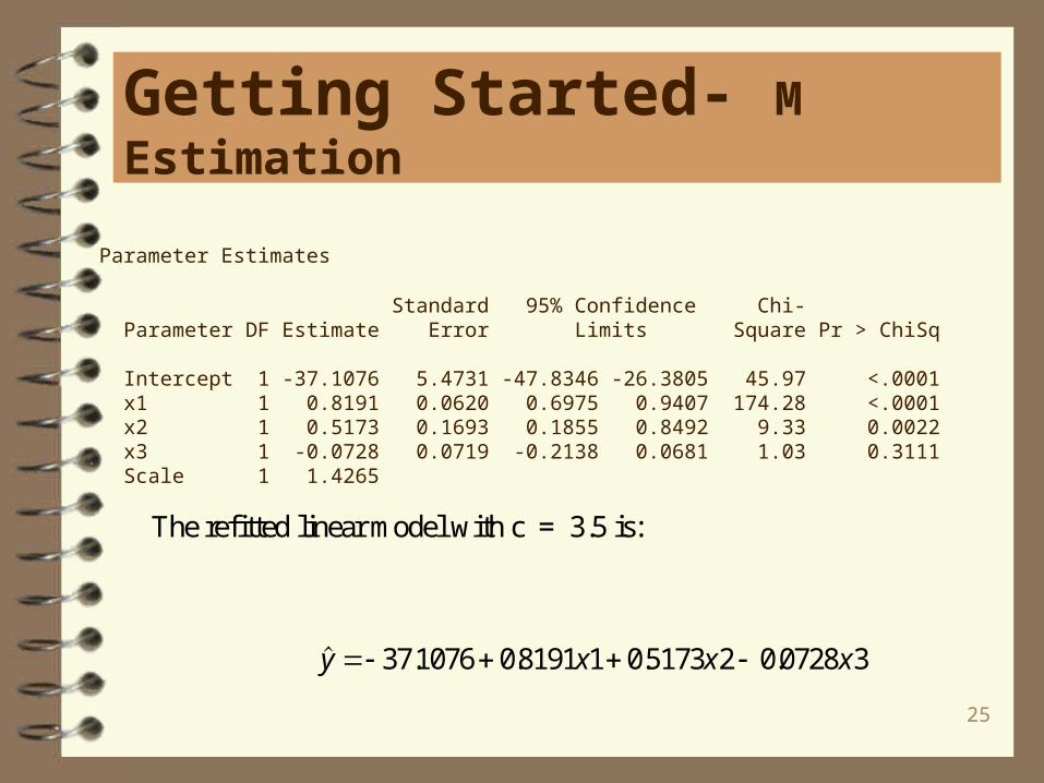
Getting Started- M Estimation
Parameter Estimates
Standard 95% Confidence Chi- Parameter DF Estimate Error Limits Square Pr > ChiSq
Intercept 1 -37.1076 5.4731 -47.8346 -26.3805 45.97 <.0001 x1 1 0.8191 0.0620 0.6975 0.9407 174.28 <.0001 x2 1 0.5173 0.1693 0.1855 0.8492 9.33 0.0022 x3 1 -0.0728 0.0719 -0.2138 0.0681 1.03 0.3111 Scale 1 1.4265
The refitted linear model with c = 3.5 is:
. . . .y x x x 371076 08191 1 05173 2 0 0728 3
26
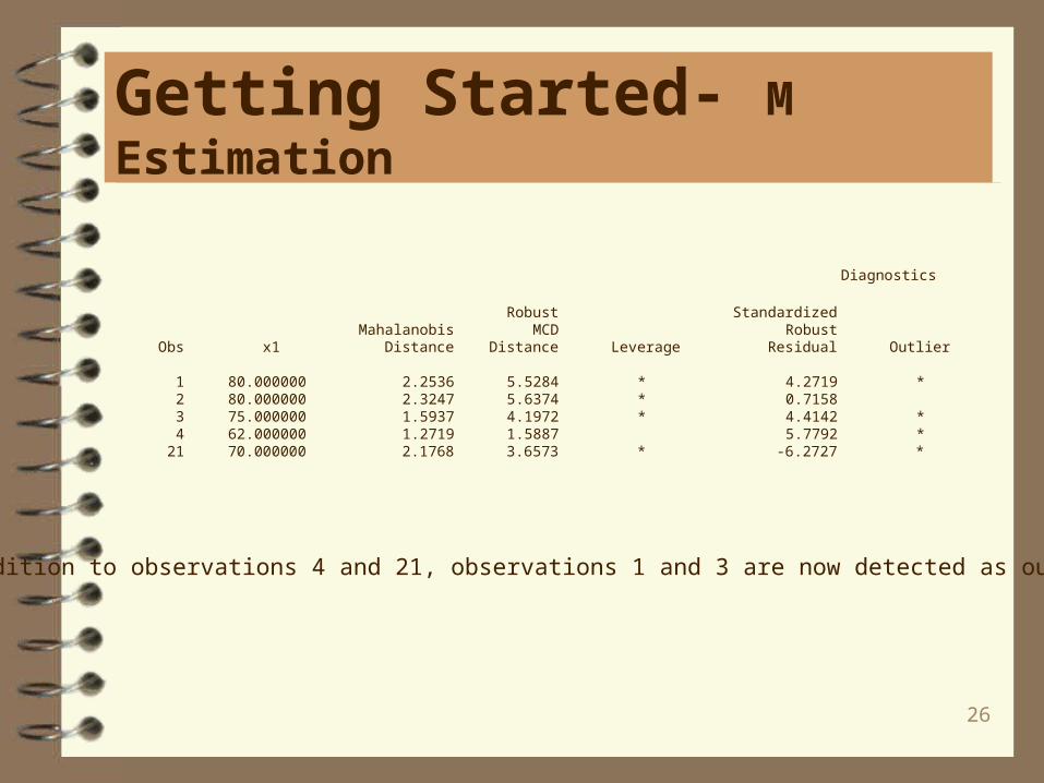
Getting Started- M Estimation
Diagnostics
Robust Standardized Mahalanobis MCD Robust Obs x1 Distance Distance Leverage Residual Outlier
1 80.000000 2.2536 5.5284 * 4.2719 * 2 80.000000 2.3247 5.6374 * 0.7158 3 75.000000 1.5937 4.1972 * 4.4142 * 4 62.000000 1.2719 1.5887 5.7792 * 21 70.000000 2.1768 3.6573 * -6.2727 *
In addition to observations 4 and 21, observations 1 and 3 are now detected as outliers.
27
Getting Started- LTS Estimation
If the data are contaminated in the x-space, M estimation does not do well. LTS estimation is more appropriate in this situation.
In the following example, the data set hbk is an artificial data set created by Hawkins, Bradu, and Kass (1984). Both OLS and M estimation suggest thatobservations 11 to 14 are serious outliers. However, these four observations weregenerated from the underlying model, whereas observations 1 to 10 were contaminated.
OLS and M estimation cannot distinguish good leverage points (observations 11to 14) from bad leverage points (observations 1 to 10). In such cases, LTS identifiesthe true outliers.
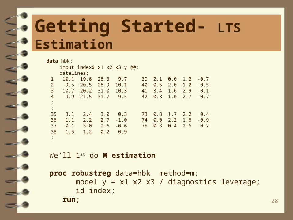
28
Getting Started- LTS Estimation
data hbk; input index$ x1 x2 x3 y @@; datalines; 1 10.1 19.6 28.3 9.7 39 2.1 0.0 1.2 -0.7 2 9.5 20.5 28.9 10.1 40 0.5 2.0 1.2 -0.5 3 10.7 20.2 31.0 10.3 41 3.4 1.6 2.9 -0.1 4 9.9 21.5 31.7 9.5 42 0.3 1.0 2.7 -0.7 : : 35 3.1 2.4 3.0 0.3 73 0.3 1.7 2.2 0.4 36 1.1 2.2 2.7 -1.0 74 0.0 2.2 1.6 -0.9 37 0.1 3.0 2.6 -0.6 75 0.3 0.4 2.6 0.2 38 1.5 1.2 0.2 0.9 ;
We’ll 1st do M estimation
proc robustreg data=hbk method=m; model y = x1 x2 x3 / diagnostics leverage; id index; run;
29
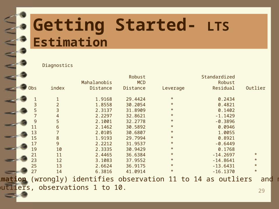
Getting Started- LTS Estimation
Diagnostics
Robust Standardized Mahalanobis MCD Robust Obs index Distance Distance Leverage Residual Outlier
1 1 1.9168 29.4424 * 0.2434 3 2 1.8558 30.2054 * 0.4821 5 3 2.3137 31.8909 * 0.1402 7 4 2.2297 32.8621 * -1.1429 9 5 2.1001 32.2778 * -0.3896 11 6 2.1462 30.5892 * 0.0946 13 7 2.0105 30.6807 * 1.0055 15 8 1.9193 29.7994 * 0.8921 17 9 2.2212 31.9537 * -0.6449 19 10 2.3335 30.9429 * 0.1768 21 11 2.4465 36.6384 * -14.2697 * 23 12 3.1083 37.9552 * -14.8641 * 25 13 2.6624 36.9175 * -13.6431 * 27 14 6.3816 41.0914 * -16.1370 *
M estimation (wrongly) identifies observation 11 to 14 as outliers and misses thereal outliers, observations 1 to 10.
30
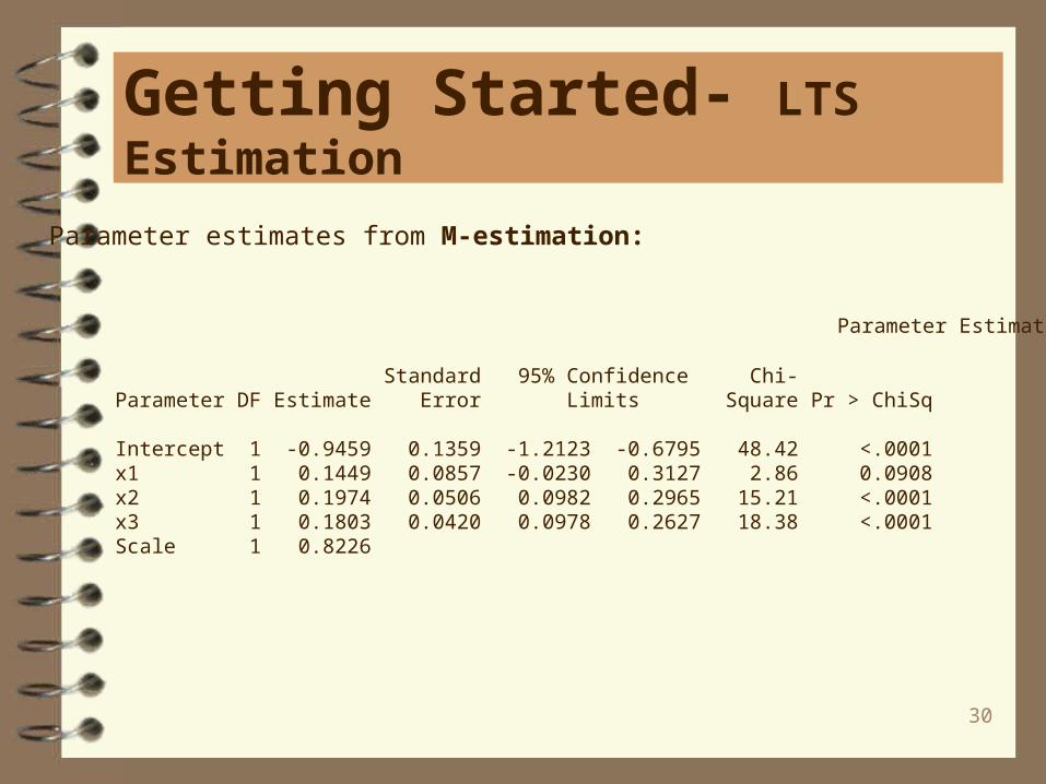
Getting Started- LTS Estimation
Parameter Estimates
Standard 95% Confidence Chi-Parameter DF Estimate Error Limits Square Pr > ChiSq
Intercept 1 -0.9459 0.1359 -1.2123 -0.6795 48.42 <.0001x1 1 0.1449 0.0857 -0.0230 0.3127 2.86 0.0908x2 1 0.1974 0.0506 0.0982 0.2965 15.21 <.0001x3 1 0.1803 0.0420 0.0978 0.2627 18.38 <.0001Scale 1 0.8226
Parameter estimates from M-estimation:
31
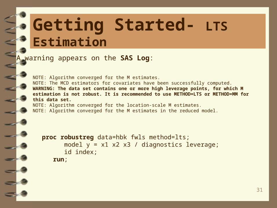
Getting Started- LTS Estimation
NOTE: Algorithm converged for the M estimates.NOTE: The MCD estimators for covariates have been successfully computed.WARNING: The data set contains one or more high leverage points, for which M estimation is not robust. It is recommended to use METHOD=LTS or METHOD=MM for this data set.NOTE: Algorithm converged for the location-scale M estimates.NOTE: Algorithm converged for the M estimates in the reduced model.
A warning appears on the SAS Log:
proc robustreg data=hbk fwls method=lts; model y = x1 x2 x3 / diagnostics leverage; id index; run;
32
Getting Started- LTS Estimation
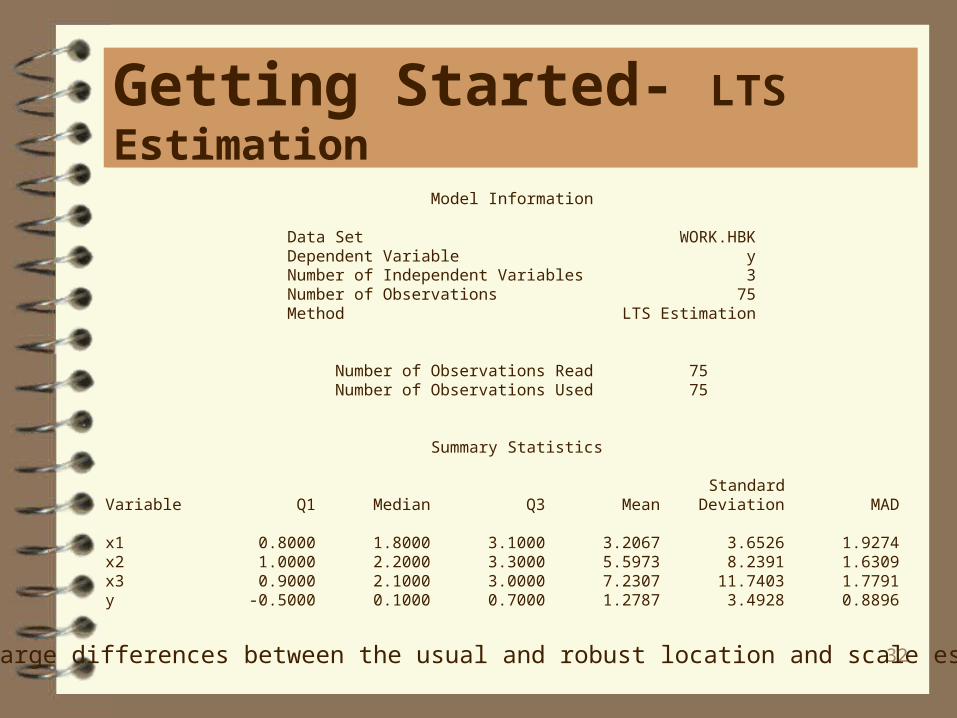
Model Information
Data Set WORK.HBK Dependent Variable y Number of Independent Variables 3 Number of Observations 75 Method LTS Estimation
Number of Observations Read 75 Number of Observations Used 75
Summary Statistics
Standard Variable Q1 Median Q3 Mean Deviation MAD
x1 0.8000 1.8000 3.1000 3.2067 3.6526 1.9274 x2 1.0000 2.2000 3.3000 5.5973 8.2391 1.6309 x3 0.9000 2.1000 3.0000 7.2307 11.7403 1.7791 y -0.5000 0.1000 0.7000 1.2787 3.4928 0.8896
Note large differences between the usual and robust location and scale estimates.
33
Getting Started- LTS Estimation
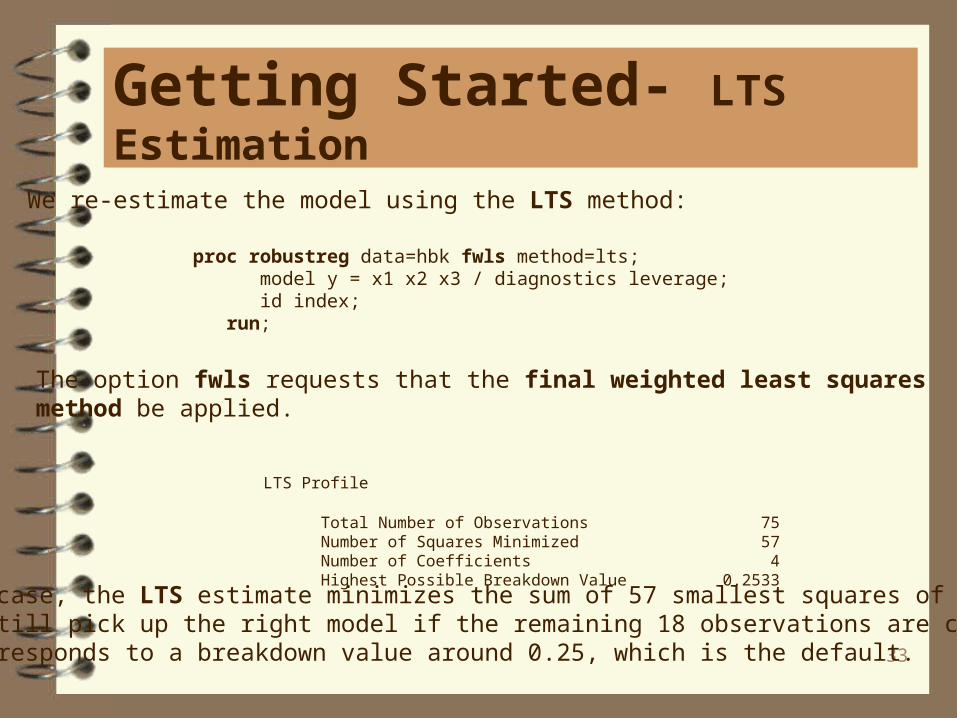
We re-estimate the model using the LTS method:
proc robustreg data=hbk fwls method=lts; model y = x1 x2 x3 / diagnostics leverage; id index; run;
The option fwls requests that the final weighted least squares method be applied.
LTS Profile
Total Number of Observations 75 Number of Squares Minimized 57 Number of Coefficients 4 Highest Possible Breakdown Value 0.2533
In this case, the LTS estimate minimizes the sum of 57 smallest squares of residuals.It can still pick up the right model if the remaining 18 observations are contaminated.This corresponds to a breakdown value around 0.25, which is the default.
34
Getting Started- LTS Estimation
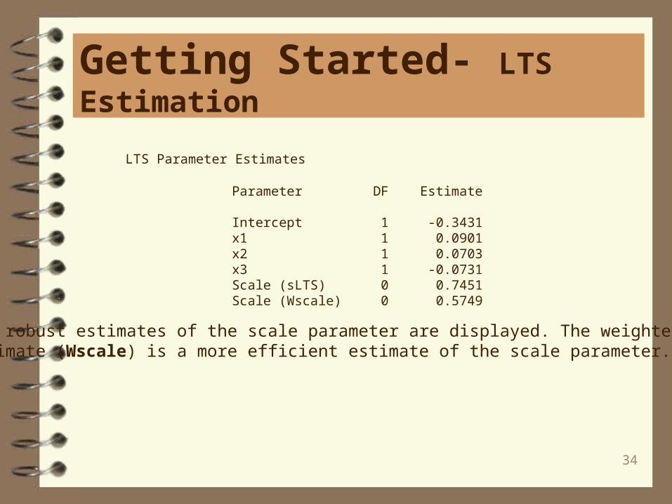
LTS Parameter Estimates
Parameter DF Estimate
Intercept 1 -0.3431 x1 1 0.0901 x2 1 0.0703 x3 1 -0.0731 Scale (sLTS) 0 0.7451 Scale (Wscale) 0 0.5749
Two robust estimates of the scale parameter are displayed. The weighted scaleestimate (Wscale) is a more efficient estimate of the scale parameter.
35
Getting Started- LTS Estimation
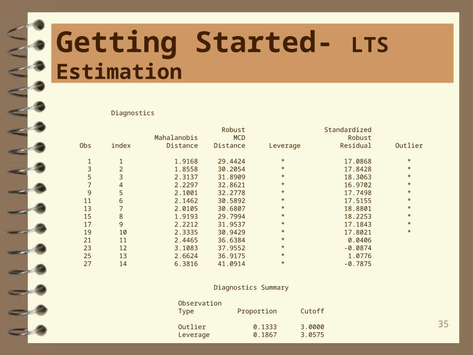
Diagnostics
Robust Standardized Mahalanobis MCD Robust Obs index Distance Distance Leverage Residual Outlier
1 1 1.9168 29.4424 * 17.0868 * 3 2 1.8558 30.2054 * 17.8428 * 5 3 2.3137 31.8909 * 18.3063 * 7 4 2.2297 32.8621 * 16.9702 * 9 5 2.1001 32.2778 * 17.7498 * 11 6 2.1462 30.5892 * 17.5155 * 13 7 2.0105 30.6807 * 18.8801 * 15 8 1.9193 29.7994 * 18.2253 * 17 9 2.2212 31.9537 * 17.1843 * 19 10 2.3335 30.9429 * 17.8021 * 21 11 2.4465 36.6384 * 0.0406 23 12 3.1083 37.9552 * -0.0874 25 13 2.6624 36.9175 * 1.0776 27 14 6.3816 41.0914 * -0.7875
Diagnostics Summary
Observation Type Proportion Cutoff
Outlier 0.1333 3.0000 Leverage 0.1867 3.0575
36
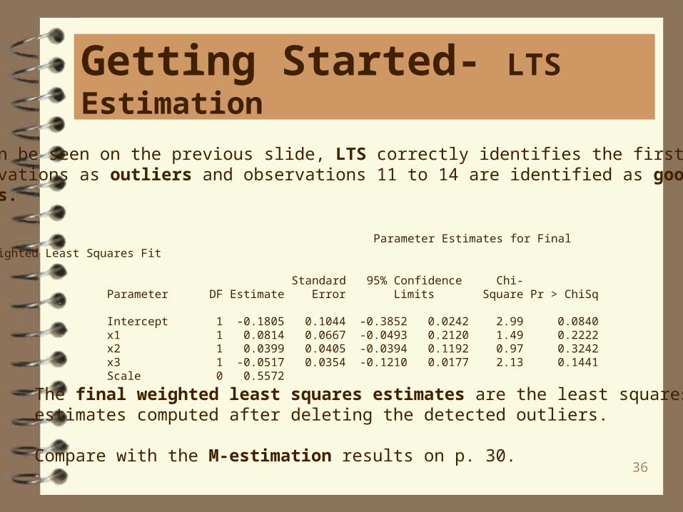
Getting Started- LTS Estimation
As can be seen on the previous slide, LTS correctly identifies the first ten observations as outliers and observations 11 to 14 are identified as good leveragepoints.
Parameter Estimates for Final Weighted Least Squares Fit
Standard 95% Confidence Chi- Parameter DF Estimate Error Limits Square Pr > ChiSq
Intercept 1 -0.1805 0.1044 -0.3852 0.0242 2.99 0.0840 x1 1 0.0814 0.0667 -0.0493 0.2120 1.49 0.2222 x2 1 0.0399 0.0405 -0.0394 0.1192 0.97 0.3242 x3 1 -0.0517 0.0354 -0.1210 0.0177 2.13 0.1441 Scale 0 0.5572
The final weighted least squares estimates are the least squares estimates computed after deleting the detected outliers.
Compare with the M-estimation results on p. 30.
37
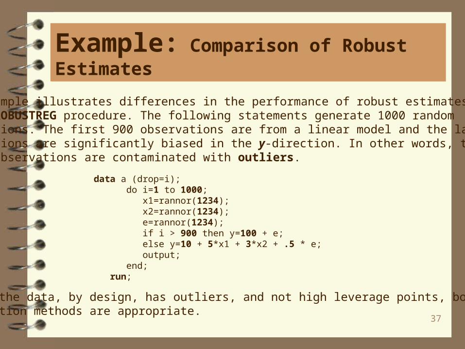
Example: Comparison of Robust Estimates
This example illustrates differences in the performance of robust estimates available in the ROBUSTREG procedure. The following statements generate 1000 random observations. The first 900 observations are from a linear model and the last 100 observations are significantly biased in the y-direction. In other words, ten percent of the observations are contaminated with outliers.
data a (drop=i); do i=1 to 1000; x1=rannor(1234); x2=rannor(1234); e=rannor(1234); if i > 900 then y=100 + e; else y=10 + 5*x1 + 3*x2 + .5 * e; output; end; run;
Since the data, by design, has outliers, and not high leverage points, both M and MMestimation methods are appropriate.
38
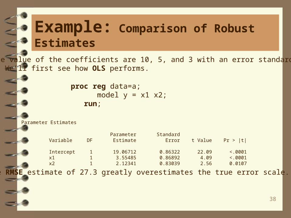
Example: Comparison of Robust Estimates
The true value of the coefficients are 10, 5, and 3 with an error standard deviationof 0.5. We’ll first see how OLS performs.
proc reg data=a; model y = x1 x2; run;
Parameter Estimates
Parameter Standard Variable DF Estimate Error t Value Pr > |t|
Intercept 1 19.06712 0.86322 22.09 <.0001 x1 1 3.55485 0.86892 4.09 <.0001 x2 1 2.12341 0.83039 2.56 0.0107
The RMSE estimate of 27.3 greatly overestimates the true error scale.

39
Example: Comparison of Robust Estimates
proc robustreg data=a method=m ; model y = x1 x2; run;
M estimation with 10% contamination:
Parameter Estimates
Standard 95% Confidence Chi- Parameter DF Estimate Error Limits Square Pr > ChiSq
Intercept 1 10.0024 0.0174 9.9683 10.0364 331908 <.0001 x1 1 5.0077 0.0175 4.9735 5.0420 82106.9 <.0001 x2 1 3.0161 0.0167 2.9834 3.0488 32612.5 <.0001 Scale 1 0.5780
Diagnostics Summary
Observation Type Proportion Cutoff
Outlier 0.1020 3.0000
40
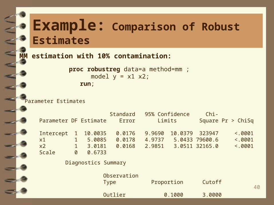
Example: Comparison of Robust Estimates
MM estimation with 10% contamination:
proc robustreg data=a method=mm ; model y = x1 x2; run;
Parameter Estimates
Standard 95% Confidence Chi- Parameter DF Estimate Error Limits Square Pr > ChiSq
Intercept 1 10.0035 0.0176 9.9690 10.0379 323947 <.0001 x1 1 5.0085 0.0178 4.9737 5.0433 79600.6 <.0001 x2 1 3.0181 0.0168 2.9851 3.0511 32165.0 <.0001 Scale 0 0.6733
Diagnostics Summary
Observation Type Proportion Cutoff
Outlier 0.1000 3.0000
41
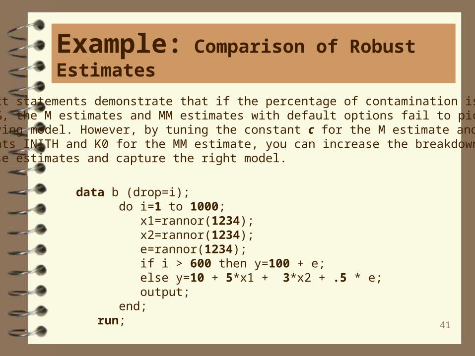
Example: Comparison of Robust Estimates
The next statements demonstrate that if the percentage of contamination is increased to 40 %, the M estimates and MM estimates with default options fail to pick up the underlying model. However, by tuning the constant c for the M estimate and the constants INITH and K0 for the MM estimate, you can increase the breakdown values of these estimates and capture the right model.
data b (drop=i); do i=1 to 1000; x1=rannor(1234); x2=rannor(1234); e=rannor(1234); if i > 600 then y=100 + e; else y=10 + 5*x1 + 3*x2 + .5 * e; output; end; run;
42
Example: Comparison of Robust Estimates
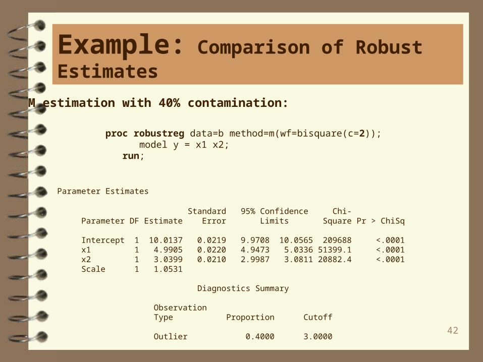
Parameter Estimates
Standard 95% Confidence Chi- Parameter DF Estimate Error Limits Square Pr > ChiSq
Intercept 1 10.0137 0.0219 9.9708 10.0565 209688 <.0001 x1 1 4.9905 0.0220 4.9473 5.0336 51399.1 <.0001 x2 1 3.0399 0.0210 2.9987 3.0811 20882.4 <.0001 Scale 1 1.0531
Diagnostics Summary
Observation Type Proportion Cutoff
Outlier 0.4000 3.0000
M estimation with 40% contamination:
proc robustreg data=b method=m(wf=bisquare(c=2)); model y = x1 x2; run;

43
Example: Comparison of Robust Estimates
MM estimation with 40% contamination:
proc robustreg data=b method=mm(inith=502 k0=1.8); model y = x1 x2; run;
Parameter Estimates
Standard 95% Confidence Chi- Parameter DF Estimate Error Limits Square Pr > ChiSq
Intercept 1 10.0103 0.0213 9.9686 10.0520 221639 <.0001 x1 1 4.9890 0.0218 4.9463 5.0316 52535.9 <.0001 x2 1 3.0363 0.0201 2.9970 3.0756 22895.5 <.0001 Scale 0 1.8992
Diagnostics Summary
Observation Type Proportion Cutoff
Outlier 0.4000 3.0000
44
Example: Comparison of Robust Estimates
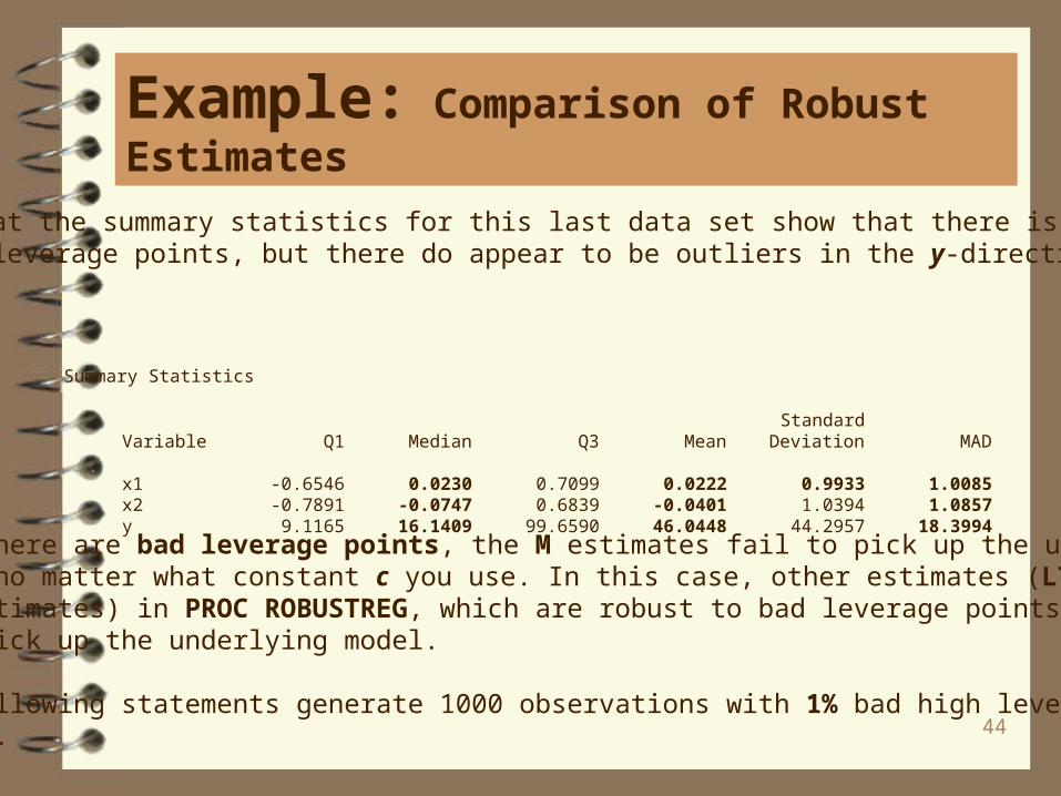
When there are bad leverage points, the M estimates fail to pick up the underlying model no matter what constant c you use. In this case, other estimates (LTS, S, and MM estimates) in PROC ROBUSTREG, which are robust to bad leverage points, will pick up the underlying model.
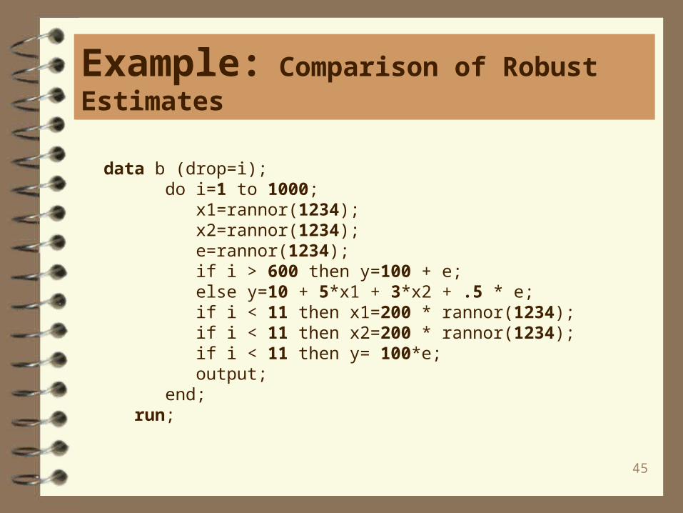
The following statements generate 1000 observations with 1% bad high leverage points.
Note that the summary statistics for this last data set show that there is no evidenceof any leverage points, but there do appear to be outliers in the y-direction.
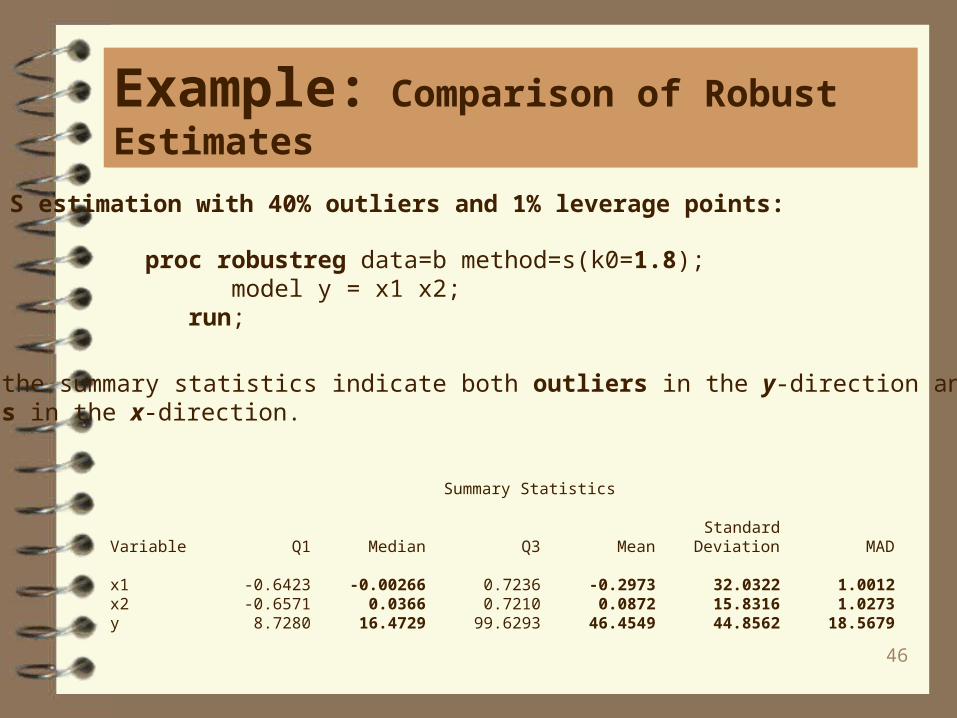
Summary Statistics
Standard Variable Q1 Median Q3 Mean Deviation MAD
x1 -0.6546 0.0230 0.7099 0.0222 0.9933 1.0085 x2 -0.7891 -0.0747 0.6839 -0.0401 1.0394 1.0857 y 9.1165 16.1409 99.6590 46.0448 44.2957 18.3994
45
Example: Comparison of Robust Estimates
data b (drop=i); do i=1 to 1000; x1=rannor(1234); x2=rannor(1234); e=rannor(1234); if i > 600 then y=100 + e; else y=10 + 5*x1 + 3*x2 + .5 * e; if i < 11 then x1=200 * rannor(1234); if i < 11 then x2=200 * rannor(1234); if i < 11 then y= 100*e; output; end; run;
46
Example: Comparison of Robust Estimates
Summary Statistics
Standard Variable Q1 Median Q3 Mean Deviation MAD
x1 -0.6423 -0.00266 0.7236 -0.2973 32.0322 1.0012 x2 -0.6571 0.0366 0.7210 0.0872 15.8316 1.0273 y 8.7280 16.4729 99.6293 46.4549 44.8562 18.5679
S estimation with 40% outliers and 1% leverage points:
proc robustreg data=b method=s(k0=1.8); model y = x1 x2; run;
Note the summary statistics indicate both outliers in the y-direction and leveragepoints in the x-direction.
47
Example: Comparison of Robust Estimates
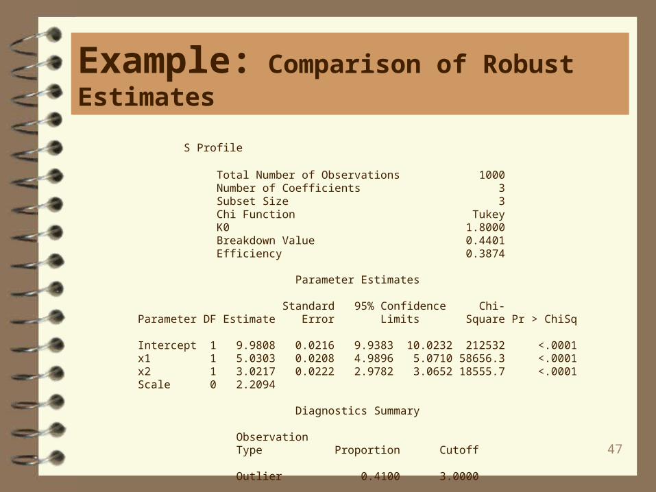
S Profile
Total Number of Observations 1000 Number of Coefficients 3 Subset Size 3 Chi Function Tukey K0 1.8000 Breakdown Value 0.4401 Efficiency 0.3874
Parameter Estimates
Standard 95% Confidence Chi- Parameter DF Estimate Error Limits Square Pr > ChiSq
Intercept 1 9.9808 0.0216 9.9383 10.0232 212532 <.0001 x1 1 5.0303 0.0208 4.9896 5.0710 58656.3 <.0001 x2 1 3.0217 0.0222 2.9782 3.0652 18555.7 <.0001 Scale 0 2.2094
Diagnostics Summary
Observation Type Proportion Cutoff
Outlier 0.4100 3.0000
48
Example: Comparison of Robust Estimates
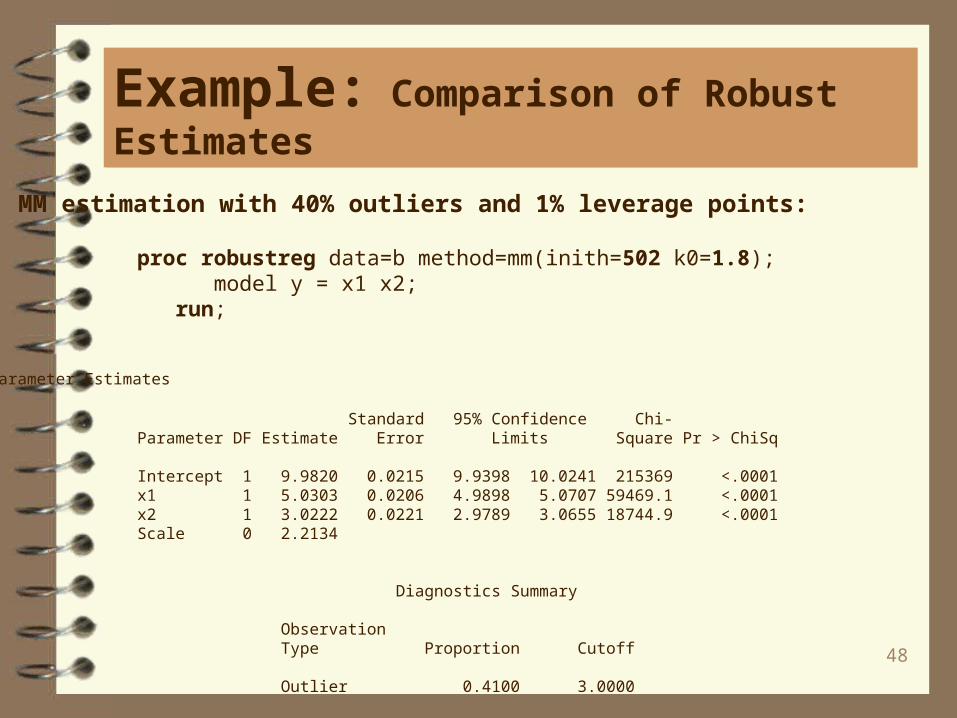
MM estimation with 40% outliers and 1% leverage points:
proc robustreg data=b method=mm(inith=502 k0=1.8); model y = x1 x2; run;
Parameter Estimates
Standard 95% Confidence Chi- Parameter DF Estimate Error Limits Square Pr > ChiSq
Intercept 1 9.9820 0.0215 9.9398 10.0241 215369 <.0001 x1 1 5.0303 0.0206 4.9898 5.0707 59469.1 <.0001 x2 1 3.0222 0.0221 2.9789 3.0655 18744.9 <.0001 Scale 0 2.2134
Diagnostics Summary
Observation Type Proportion Cutoff
Outlier 0.4100 3.0000
49
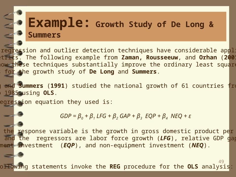
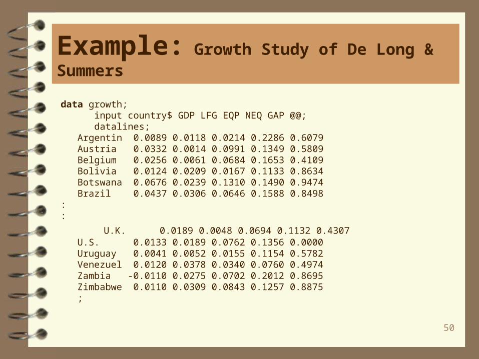
Example: Growth Study of De Long & Summers
Robust regression and outlier detection techniques have considerable applications to econometrics. The following example from Zaman, Rousseeuw, and Orhan (2001) shows how these techniques substantially improve the ordinary least squares (OLS) results for the growth study of De Long and Summers.
De Long and Summers (1991) studied the national growth of 61 countries from 1960 to 1985 using OLS.
The regression equation they used is:
GDP = β0 + β1 LFG + β2 GAP + β3 EQP + β4 NEQ + ε
where the response variable is the growth in gross domestic product per worker (GDP) and the regressors are labor force growth (LFG), relative GDP gap (GAP), equipment investment (EQP), and non-equipment investment (NEQ).
The following statements invoke the REG procedure for the OLS analysis:
50
Example: Growth Study of De Long & Summers
data growth; input country$ GDP LFG EQP NEQ GAP @@; datalines; Argentin 0.0089 0.0118 0.0214 0.2286 0.6079 Austria 0.0332 0.0014 0.0991 0.1349 0.5809 Belgium 0.0256 0.0061 0.0684 0.1653 0.4109 Bolivia 0.0124 0.0209 0.0167 0.1133 0.8634 Botswana 0.0676 0.0239 0.1310 0.1490 0.9474 Brazil 0.0437 0.0306 0.0646 0.1588 0.8498 ::
U.K. 0.0189 0.0048 0.0694 0.1132 0.4307 U.S. 0.0133 0.0189 0.0762 0.1356 0.0000 Uruguay 0.0041 0.0052 0.0155 0.1154 0.5782 Venezuel 0.0120 0.0378 0.0340 0.0760 0.4974 Zambia -0.0110 0.0275 0.0702 0.2012 0.8695 Zimbabwe 0.0110 0.0309 0.0843 0.1257 0.8875 ;
51
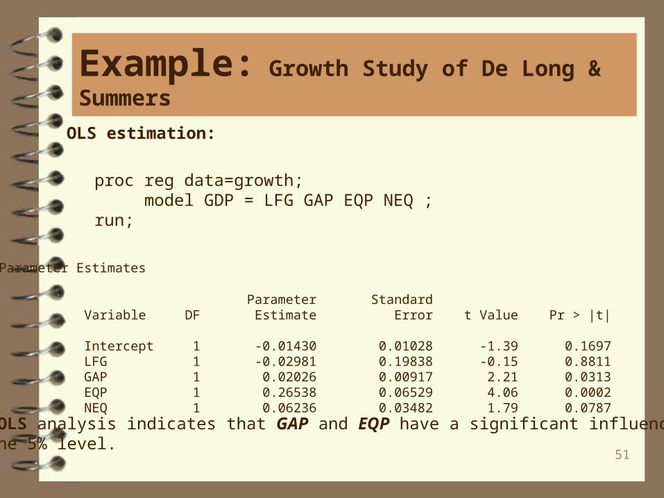
Example: Growth Study of De Long & Summers
proc reg data=growth; model GDP = LFG GAP EQP NEQ ; run;
Parameter Estimates
Parameter Standard Variable DF Estimate Error t Value Pr > |t|
Intercept 1 -0.01430 0.01028 -1.39 0.1697 LFG 1 -0.02981 0.19838 -0.15 0.8811 GAP 1 0.02026 0.00917 2.21 0.0313 EQP 1 0.26538 0.06529 4.06 0.0002 NEQ 1 0.06236 0.03482 1.79 0.0787
The OLS analysis indicates that GAP and EQP have a significant influence on GDPat the 5% level.
OLS estimation:

52
Example: Growth Study of De Long & Summers
M estimation (the default):
proc robustreg data=growth; model GDP = LFG GAP EQP NEQ / diagnostics leverage; output out=robout r=resid sr=stdres; run;
Summary Statistics
Standard Variable Q1 Median Q3 Mean Deviation MAD
LFG 0.0118 0.0239 0.0281 0.0211 0.00979 0.00949 GAP 0.5796 0.8015 0.8863 0.7258 0.2181 0.1778 EQP 0.0265 0.0433 0.0720 0.0523 0.0296 0.0325 NEQ 0.0956 0.1356 0.1812 0.1399 0.0570 0.0624 GDP 0.0121 0.0231 0.0310 0.0224 0.0155 0.0150
It’s not obvious from the summary statistics that there may be outliers or leveragepoints.
53
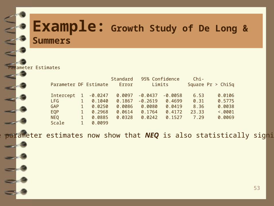
Example: Growth Study of De Long & Summers
Parameter Estimates
Standard 95% Confidence Chi- Parameter DF Estimate Error Limits Square Pr > ChiSq
Intercept 1 -0.0247 0.0097 -0.0437 -0.0058 6.53 0.0106 LFG 1 0.1040 0.1867 -0.2619 0.4699 0.31 0.5775 GAP 1 0.0250 0.0086 0.0080 0.0419 8.36 0.0038 EQP 1 0.2968 0.0614 0.1764 0.4172 23.33 <.0001 NEQ 1 0.0885 0.0328 0.0242 0.1527 7.29 0.0069 Scale 1 0.0099
The parameter estimates now show that NEQ is also statistically significant.
54
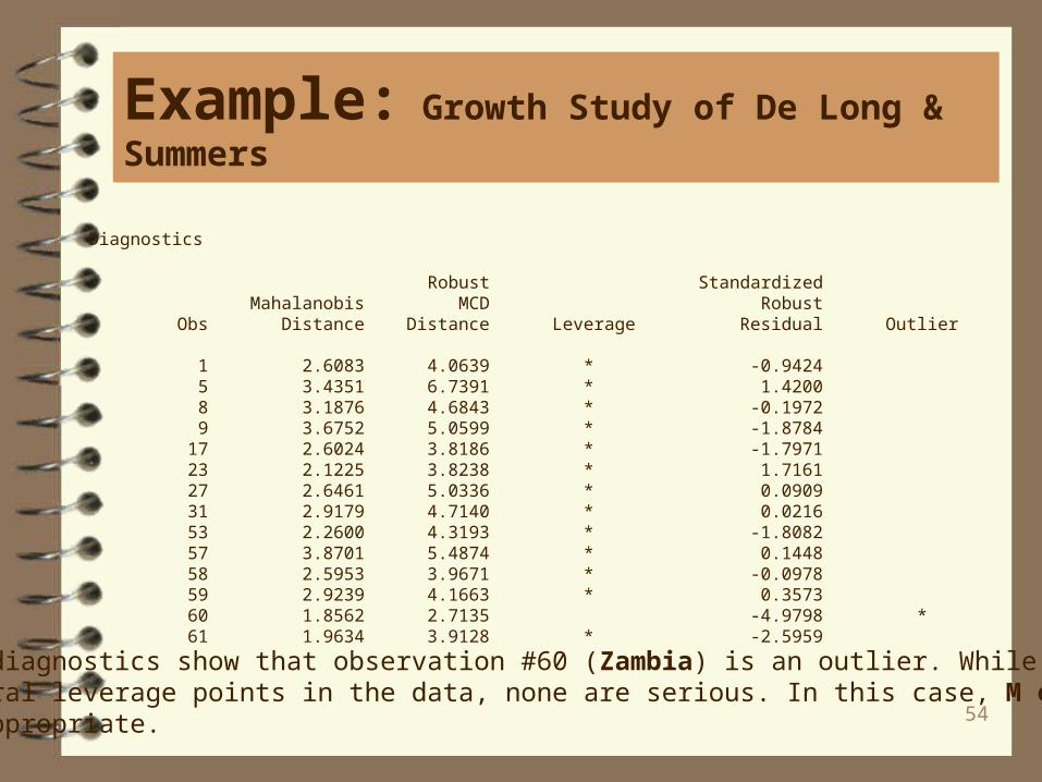
Example: Growth Study of De Long & Summers
Diagnostics
Robust Standardized Mahalanobis MCD Robust Obs Distance Distance Leverage Residual Outlier
1 2.6083 4.0639 * -0.9424 5 3.4351 6.7391 * 1.4200 8 3.1876 4.6843 * -0.1972 9 3.6752 5.0599 * -1.8784 17 2.6024 3.8186 * -1.7971 23 2.1225 3.8238 * 1.7161 27 2.6461 5.0336 * 0.0909 31 2.9179 4.7140 * 0.0216 53 2.2600 4.3193 * -1.8082 57 3.8701 5.4874 * 0.1448 58 2.5953 3.9671 * -0.0978 59 2.9239 4.1663 * 0.3573 60 1.8562 2.7135 -4.9798 * 61 1.9634 3.9128 * -2.5959
The diagnostics show that observation #60 (Zambia) is an outlier. While there areseveral leverage points in the data, none are serious. In this case, M estimationis appropriate.
55
Example: Growth Study of De Long & Summers
The following statements invoke the ROBUSTREG procedure with LTS estimation, which was used by Zaman, Rousseeuw, and Orhan (2001). The results are consistent with those of M estimation.
proc robustreg method=lts(h=33) fwls data=growth; model GDP = LFG GAP EQP NEQ / diagnostics leverage ; output out=robout r=resid sr=stdres;
run;

56
Example: Growth Study of De Long & Summers
Parameter Estimates for Final Weighted Least Squares Fit
Standard 95% Confidence Chi- Parameter DF Estimate Error Limits Square Pr > ChiSq
Intercept 1 -0.0222 0.0093 -0.0405 -0.0039 5.65 0.0175 LFG 1 0.0446 0.1771 -0.3026 0.3917 0.06 0.8013 GAP 1 0.0245 0.0082 0.0084 0.0406 8.89 0.0029 EQP 1 0.2824 0.0581 0.1685 0.3964 23.60 <.0001 NEQ 1 0.0849 0.0314 0.0233 0.1465 7.30 0.0069 Scale 0 0.0116
The final weighted lease squares estimates are identical to those reported in Zaman, Rousseeuw, and Orhan (2001).


![Robust Detection of Copy Move Forgery in Color Imagesworldcomp-proceedings.com/proc/p2013/IPC4111.pdf · 2014. 4. 16. · Weiqi Luo et al. [6] presented a technique . robust to various](https://static.fdocuments.in/doc/165x107/61385eef0ad5d20676493683/robust-detection-of-copy-move-forgery-in-color-imagesworldcomp-2014-4-16-weiqi.jpg)