
Problem Set II - Massachusetts Institute of Technologypeople.csail.mit.edu/halordain/2D...
18
Christopher Tsai December 26, 2007 EE 262 – 2D Imaging Page | 1 Problem Set II – Coherent and Incoherent Imaging Problem #1 – Digital Elevation Model We first generate a digital elevation model (DEM) of the big island of Hawaii to examine the topography cursorily: The two larger red spots represent Hawaii’s tallest peaks, Mauna Kea in the north and Mauna Loa in the south. To quantify the heights more precisely, however, we must plot the contours: Problem 1A - Digital Elevation Model for Big Island of Hawaii 100 200 300 400 500 600 700 100 200 300 400 500 600 700 800 900 0 500 1000 1500 2000 2500 3000 3500 4000
Transcript of Problem Set II - Massachusetts Institute of Technologypeople.csail.mit.edu/halordain/2D...
Christopher Tsai December 26, 2007
EE 262 – 2D Imaging
Page | 1
Problem Set II – Coherent and Incoherent Imaging
Problem #1 – Digital Elevation Model
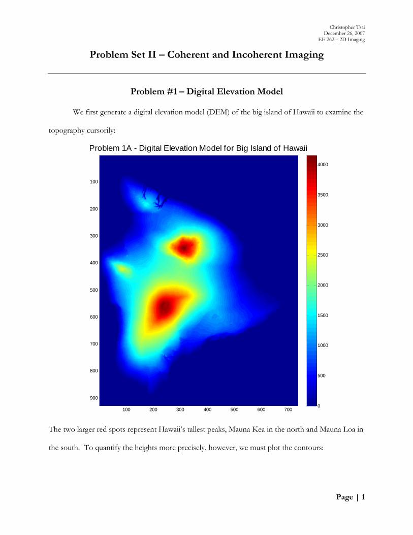
We first generate a digital elevation model (DEM) of the big island of Hawaii to examine the
topography cursorily:
The two larger red spots represent Hawaii’s tallest peaks, Mauna Kea in the north and Mauna Loa in
the south. To quantify the heights more precisely, however, we must plot the contours:
Problem 1A - Digital Elevation Model for Big Island of Hawaii
100 200 300 400 500 600 700
100
200
300
400
500
600
700
800
9000
500
1000
1500
2000
2500
3000
3500
4000
Christopher Tsai December 26, 2007
EE 262 – 2D Imaging
Page | 2
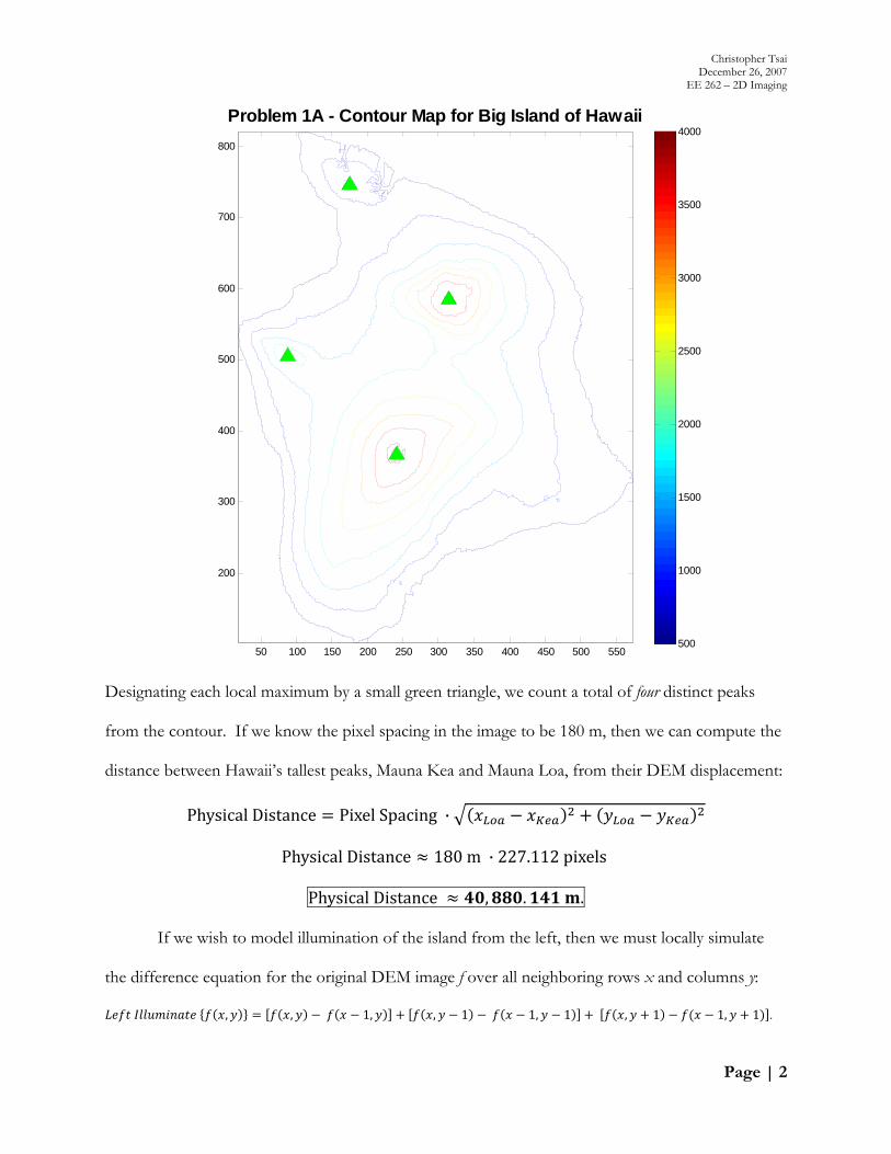
Designating each local maximum by a small green triangle, we count a total of four distinct peaks
from the contour. If we know the pixel spacing in the image to be 180 m, then we can compute the
distance between Hawaii’s tallest peaks, Mauna Kea and Mauna Loa, from their DEM displacement:
Physical Distance Pixel Spacing ·
Physical Distance 180 m · 227.112 pixels
Physical Distance , . .
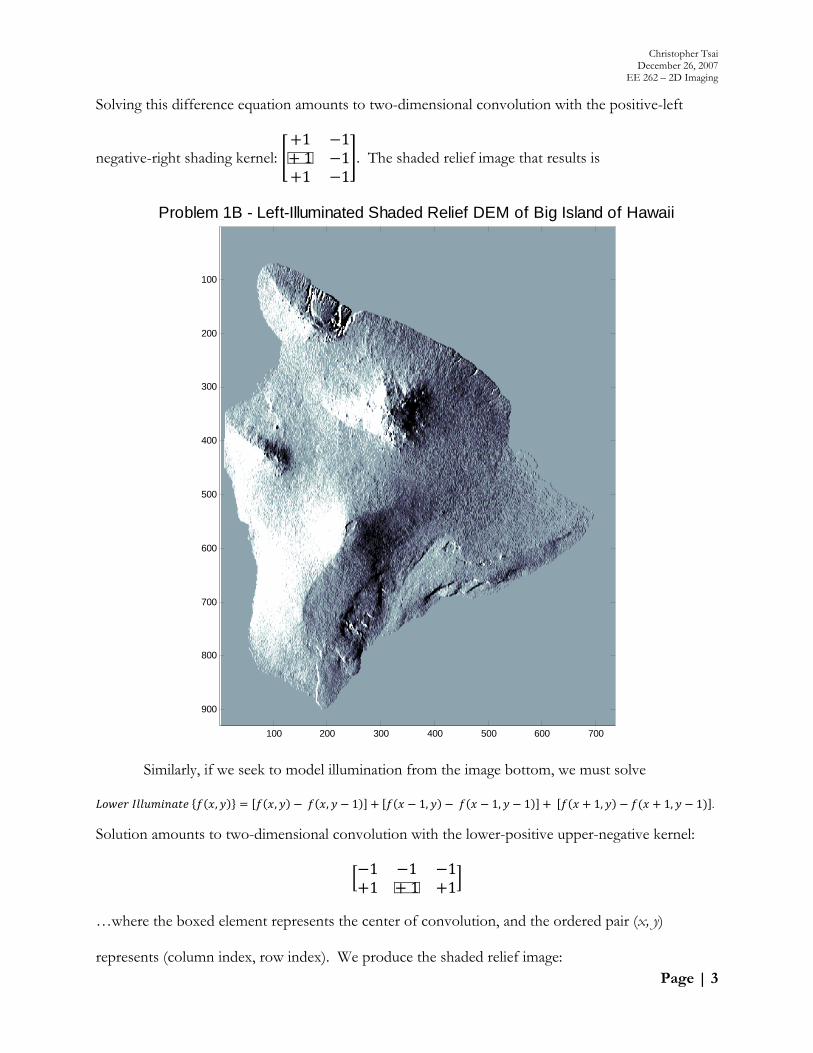
If we wish to model illumination of the island from the left, then we must locally simulate
the difference equation for the original DEM image f over all neighboring rows x and columns y:
, , 1, , 1 1, 1 , 1 1, 1 .
Problem 1A - Contour Map for Big Island of Hawaii
50 100 150 200 250 300 350 400 450 500 550
200
300
400
500
600
700
800
500
1000
1500
2000
2500
3000
3500
4000
Christopher Tsai December 26, 2007
EE 262 – 2D Imaging
Page | 3
Solving this difference equation amounts to two-dimensional convolution with the positive-left
negative-right shading kernel: 1 11 11 1
. The shaded relief image that results is
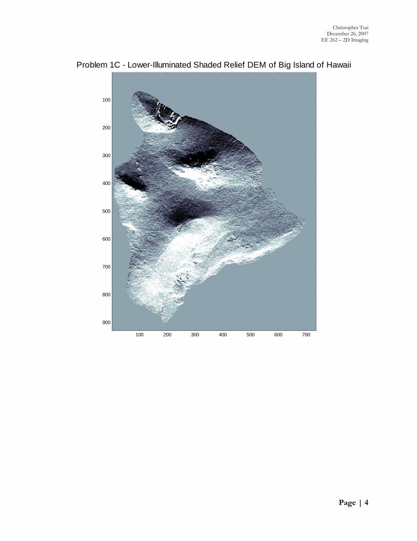
Similarly, if we seek to model illumination from the image bottom, we must solve
, , , 1 1, 1, 1 1, 1, 1 .
Solution amounts to two-dimensional convolution with the lower-positive upper-negative kernel:
1 1 11 1 1
…where the boxed element represents the center of convolution, and the ordered pair (x, y)
represents (column index, row index). We produce the shaded relief image:
Problem 1B - Left-Illuminated Shaded Relief DEM of Big Island of Hawaii
100 200 300 400 500 600 700
100
200
300
400
500
600
700
800
900
Christopher Tsai December 26, 2007
EE 262 – 2D Imaging
Page | 4
Problem 1C - Lower-Illuminated Shaded Relief DEM of Big Island of Hawaii
100 200 300 400 500 600 700
100
200
300
400
500
600
700
800
900
Christopher Tsai December 26, 2007
EE 262 – 2D Imaging
Page | 5
Problem #2 – Perspective Projection
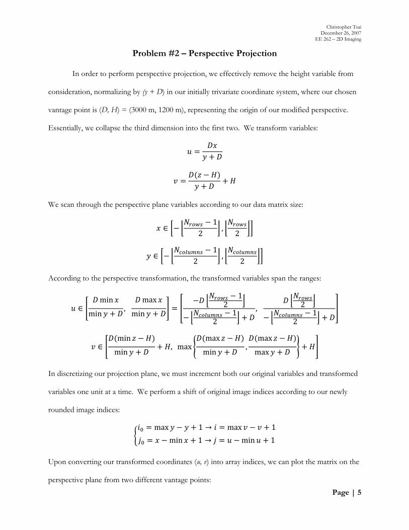
In order to perform perspective projection, we effectively remove the height variable from
consideration, normalizing by (y + D) in our initially trivariate coordinate system, where our chosen
vantage point is (D, H) = (3000 m, 1200 m), representing the origin of our modified perspective.
Essentially, we collapse the third dimension into the first two. We transform variables:
We scan through the perspective plane variables according to our data matrix size:
12 , 2
12 , 2
According to the perspective transformation, the transformed variables span the ranges:
min
min , max
min
12
12
, 21
2
min
min , maxmax
min ,max
max
In discretizing our projection plane, we must increment both our original variables and transformed
variables one unit at a time. We perform a shift of original image indices according to our newly
rounded image indices:
max 1 max 1min 1 min 1
Upon converting our transformed coordinates (u, v) into array indices, we can plot the matrix on the
perspective plane from two different vantage points:
Christopher Tsai December 26, 2007
EE 262 – 2D Imaging
Page | 6
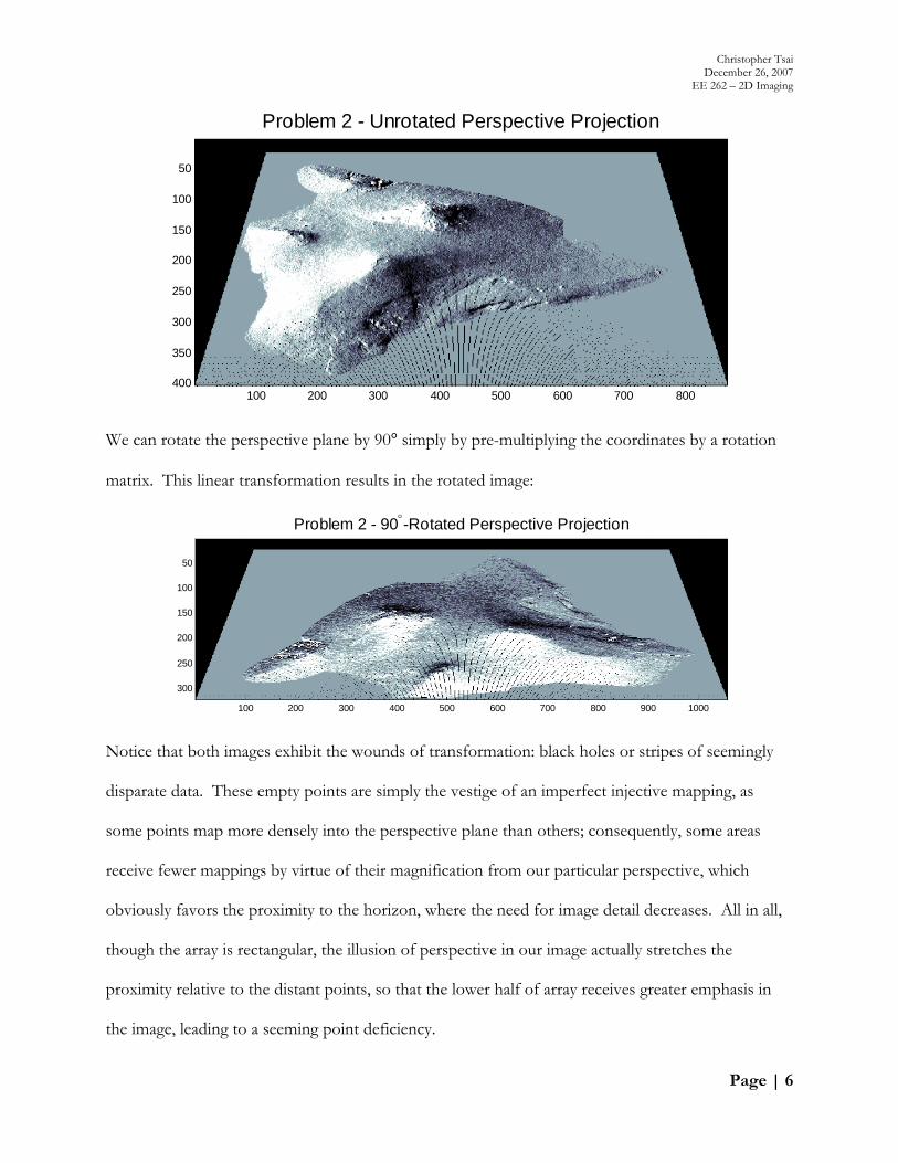
We can rotate the perspective plane by 90° simply by pre-multiplying the coordinates by a rotation
matrix. This linear transformation results in the rotated image:
Notice that both images exhibit the wounds of transformation: black holes or stripes of seemingly
disparate data. These empty points are simply the vestige of an imperfect injective mapping, as
some points map more densely into the perspective plane than others; consequently, some areas
receive fewer mappings by virtue of their magnification from our particular perspective, which
obviously favors the proximity to the horizon, where the need for image detail decreases. All in all,
though the array is rectangular, the illusion of perspective in our image actually stretches the
proximity relative to the distant points, so that the lower half of array receives greater emphasis in
the image, leading to a seeming point deficiency.
Problem 2 - Unrotated Perspective Projection
100 200 300 400 500 600 700 800
50
100
150
200
250
300
350
400
Problem 2 - 90°-Rotated Perspective Projection
100 200 300 400 500 600 700 800 900 1000
50
100
150
200
250
300
Christopher Tsai December 26, 2007
EE 262 – 2D Imaging
Page | 7
Problem #3 – Pinhole Camera Equations
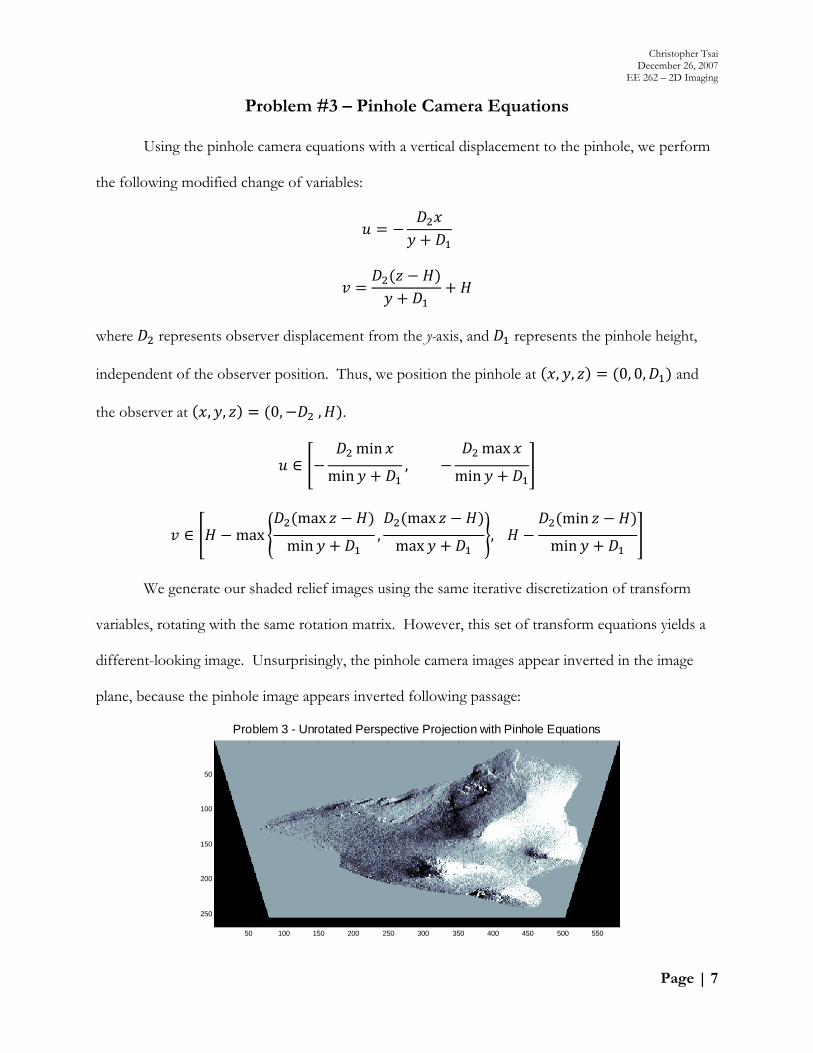
Using the pinhole camera equations with a vertical displacement to the pinhole, we perform
the following modified change of variables:
where represents observer displacement from the y-axis, and represents the pinhole height,
independent of the observer position. Thus, we position the pinhole at , , 0, 0, and
the observer at , , 0, , .
min
min ,max
min
maxmax
min ,max
max , min
min
We generate our shaded relief images using the same iterative discretization of transform
variables, rotating with the same rotation matrix. However, this set of transform equations yields a
different-looking image. Unsurprisingly, the pinhole camera images appear inverted in the image
plane, because the pinhole image appears inverted following passage:
Problem 3 - Unrotated Perspective Projection with Pinhole Equations
50 100 150 200 250 300 350 400 450 500 550
50
100
150
200
250

Christopher Tsai December 26, 2007
EE 262 – 2D Imaging
Page | 8
Problem 3 - 90°-Rotated Perspective Projection with Pinhole Equations
100 200 300 400 500 600 700
50
100
150
200
Christopher Tsai December 26, 2007
EE 262 – 2D Imaging
Page | 9
Problem #4 – Gaussian Random Number Generator
A uniform random variable ~U , has zero mean and variance σ . Thus, we
can approximate a Gaussian random vector by summing twelve vectors of these uniform random
variables. Since expectation is linear, the Gaussian mean will remain zero, while the variance of the
sum of independent random variables is the sum of the variances, thus elevating our Gaussian
variance to unity. We populate an entire vector with these independent sums, and hence produce a
string of normally distributed random numbers with zero mean and unit variance. We combine
independently drawn pairs in (C = X + jY) to produce complex Gaussian random variables. To
ensure that our complex combination’s constituents are successfully Gaussian, we measure their
means, variances, and third moments across vectors of length 1,000,000 (one million iterations), as
tabulated below:
Random Variable Mean µ Variance Third Moment
Real Part {C} = X -0.000380 0 0.999081 1 0.000197 0
Imaginary Part {C} = Y -0.000349 0 0.997051 1 -0.000846 0
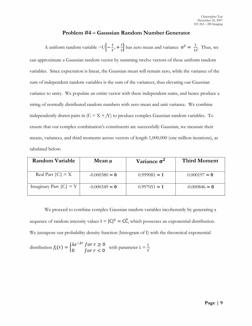
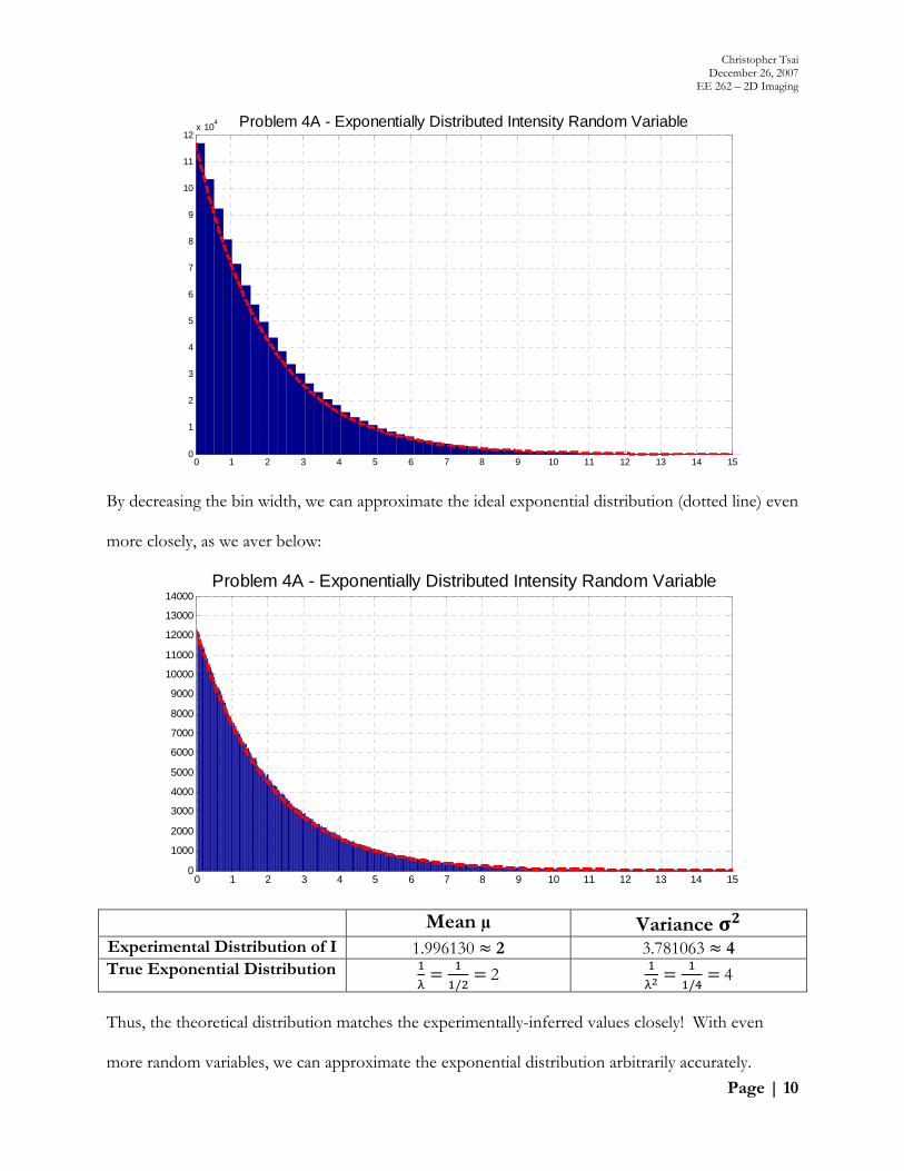
We proceed to combine complex Gaussian random variables incoherently by generating a
sequence of random intensity values I = |C| CC, which possesses an exponential distribution.
We juxtapose our probability density function (histogram of I) with the theoretical exponential
distribution I 0
0 0 with parameter λ = :
Christopher Tsai December 26, 2007
EE 262 – 2D Imaging
Page | 10
By decreasing the bin width, we can approximate the ideal exponential distribution (dotted line) even
more closely, as we aver below:
Mean µ Variance Experimental Distribution of I 1.996130 2 3.781063 4 True Exponential Distribution
/2
/ 4
Thus, the theoretical distribution matches the experimentally-inferred values closely! With even
more random variables, we can approximate the exponential distribution arbitrarily accurately.
0 1 2 3 4 5 6 7 8 9 10 11 12 13 14 150
1
2
3
4
5
6
7
8
9
10
11
12x 104 Problem 4A - Exponentially Distributed Intensity Random Variable
0 1 2 3 4 5 6 7 8 9 10 11 12 13 14 150
1000
2000
3000
4000
5000
6000
7000
8000
9000
10000
11000
12000
13000
14000Problem 4A - Exponentially Distributed Intensity Random Variable
Christopher Tsai December 26, 2007
EE 262 – 2D Imaging
Page | 11
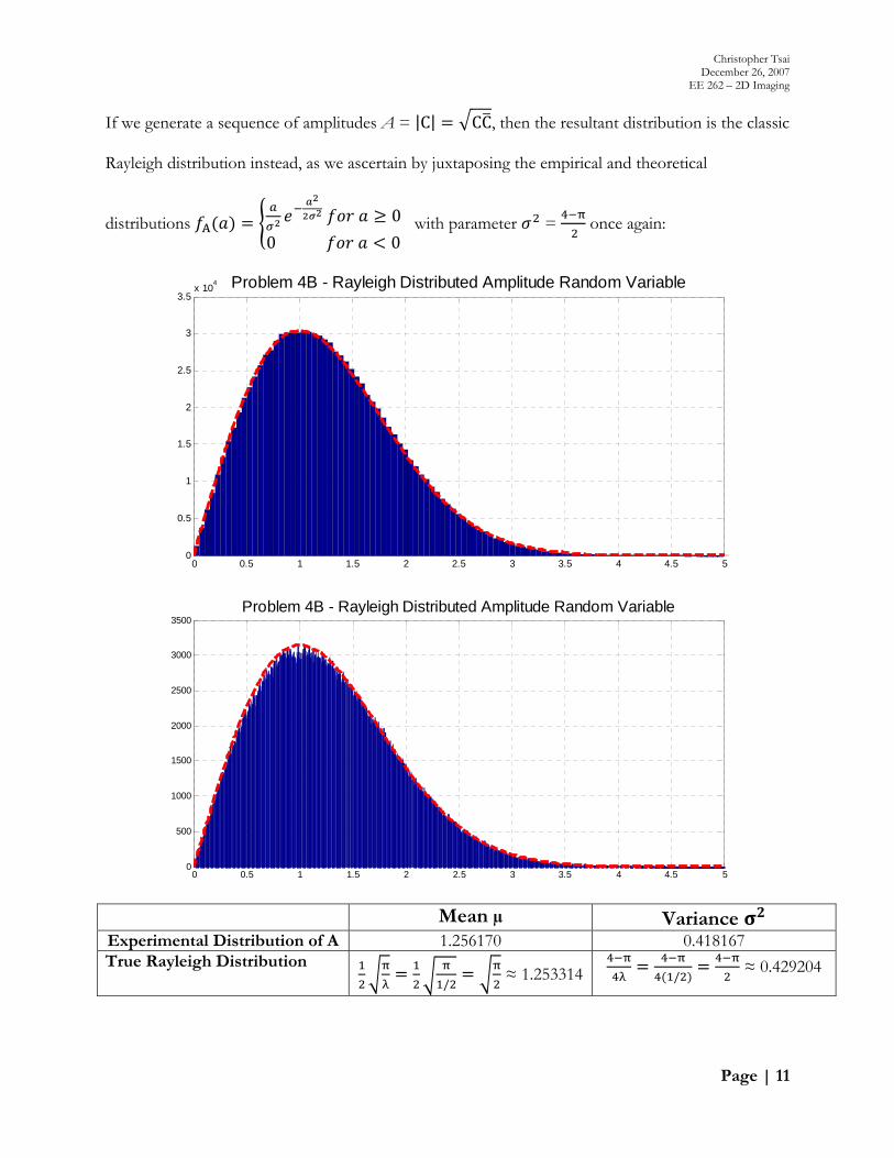
If we generate a sequence of amplitudes A = |C| CC, then the resultant distribution is the classic
Rayleigh distribution instead, as we ascertain by juxtaposing the empirical and theoretical
distributions A 0
0 0 with parameter =
once again:
Mean µ Variance Experimental Distribution of A 1.256170 0.418167 True Rayleigh Distribution
/ ≈ 1.253314 /
≈ 0.429204
0 0.5 1 1.5 2 2.5 3 3.5 4 4.5 50
0.5
1
1.5
2
2.5
3
3.5x 10⁴ Problem 4B - Rayleigh Distributed Amplitude Random Variable
0 0.5 1 1.5 2 2.5 3 3.5 4 4.5 50
500
1000
1500
2000
2500
3000
3500Problem 4B - Rayleigh Distributed Amplitude Random Variable
Christopher Tsai December 26, 2007
EE 262 – 2D Imaging
Page | 12
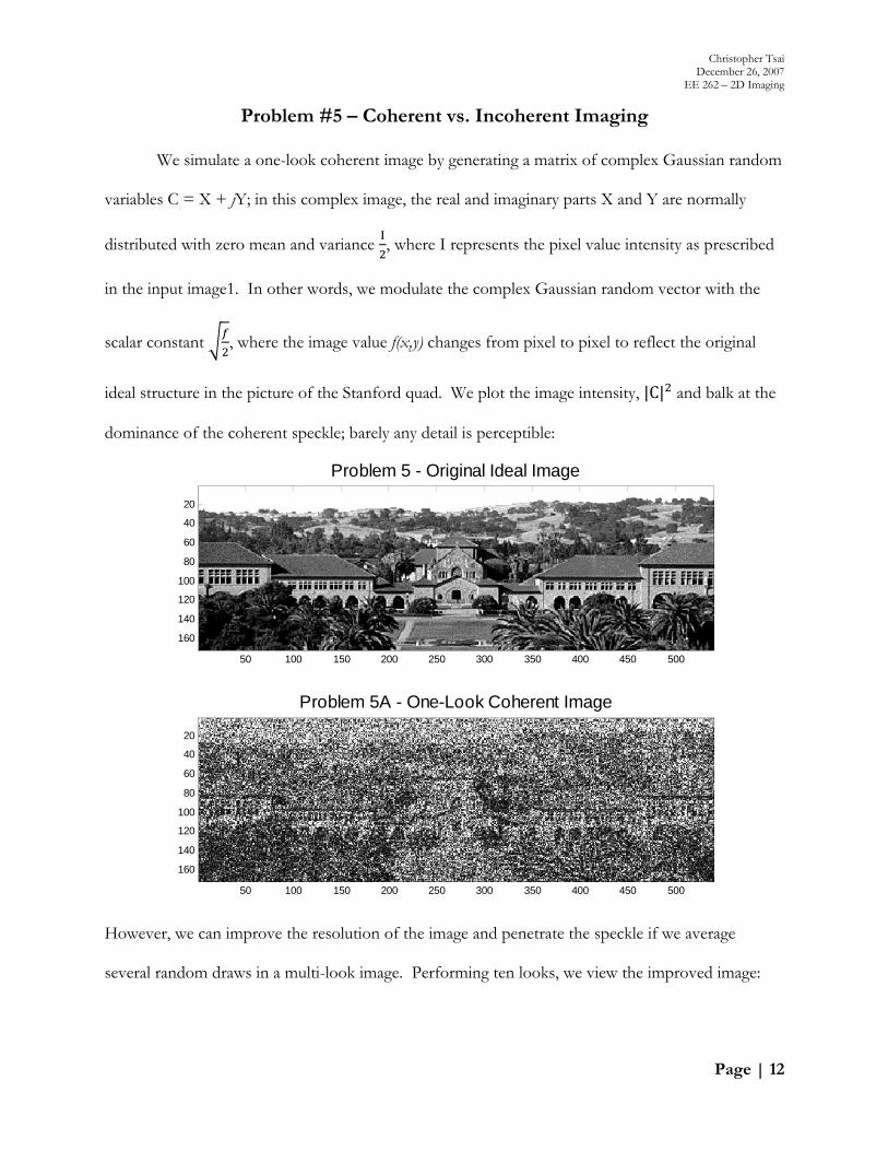
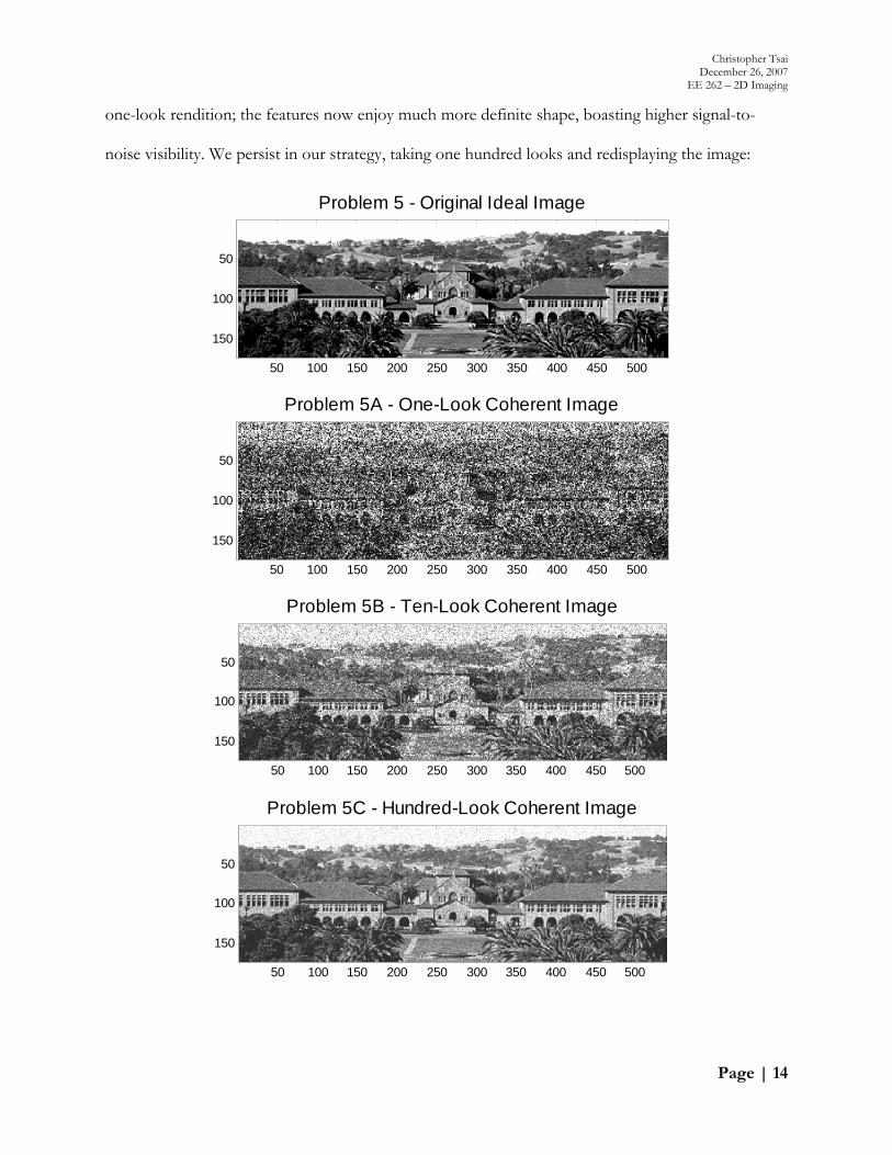
Problem #5 – Coherent vs. Incoherent Imaging
We simulate a one-look coherent image by generating a matrix of complex Gaussian random
variables C = X + jY; in this complex image, the real and imaginary parts X and Y are normally
distributed with zero mean and variance I , where I represents the pixel value intensity as prescribed
in the input image1. In other words, we modulate the complex Gaussian random vector with the
scalar constant , where the image value f(x,y) changes from pixel to pixel to reflect the original
ideal structure in the picture of the Stanford quad. We plot the image intensity, |C| and balk at the
dominance of the coherent speckle; barely any detail is perceptible:
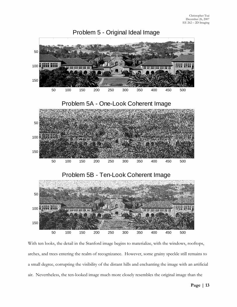
However, we can improve the resolution of the image and penetrate the speckle if we average
several random draws in a multi-look image. Performing ten looks, we view the improved image:
Problem 5 - Original Ideal Image
50 100 150 200 250 300 350 400 450 500
20
40
60
80
100
120
140
160
Problem 5A - One-Look Coherent Image
50 100 150 200 250 300 350 400 450 500
20
40
60
80
100
120
140
160
Christopher Tsai December 26, 2007
EE 262 – 2D Imaging
Page | 13
With ten looks, the detail in the Stanford image begins to materialize, with the windows, rooftops,
arches, and trees entering the realm of recognizance. However, some grainy speckle still remains to
a small degree, corrupting the visibility of the distant hills and enchanting the image with an artificial
air. Nevertheless, the ten-looked image much more closely resembles the original image than the
Problem 5 - Original Ideal Image
50 100 150 200 250 300 350 400 450 500
50
100
150
Problem 5A - One-Look Coherent Image
50 100 150 200 250 300 350 400 450 500
50
100
150
Problem 5B - Ten-Look Coherent Image
50 100 150 200 250 300 350 400 450 500
50
100
150
Christopher Tsai December 26, 2007
EE 262 – 2D Imaging
Page | 14
one-look rendition; the features now enjoy much more definite shape, boasting higher signal-to-
noise visibility. We persist in our strategy, taking one hundred looks and redisplaying the image:
Problem 5 - Original Ideal Image
50 100 150 200 250 300 350 400 450 500
50
100
150
Problem 5A - One-Look Coherent Image
50 100 150 200 250 300 350 400 450 500
50
100
150
Problem 5B - Ten-Look Coherent Image
50 100 150 200 250 300 350 400 450 500
50
100
150
Problem 5C - Hundred-Look Coherent Image
50 100 150 200 250 300 350 400 450 500
50
100
150
Christopher Tsai December 26, 2007
EE 262 – 2D Imaging
Page | 15
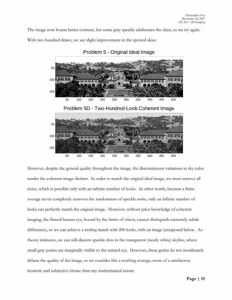
The image now boasts better contrast, but some gray speckle adulterates the skies, so we try again.
With two hundred draws, we see slight improvement in the spotted skies:
However, despite the general quality throughout the image, the discontinuous variations in sky color
render the coherent image distinct. In order to match the original ideal image, we must remove all
noise, which is possible only with an infinite number of looks. In other words, because a finite
average never completely removes the randomness of speckle noise, only an infinite number of
looks can perfectly match the original image. However, without prior knowledge of coherent
imaging, the flawed human eye, bound by the limits of vision, cannot distinguish extremely subtle
differences, so we can achieve a working match with 200 looks, with an image juxtaposed below. As
theory intimates, we can still discern speckle dots in the transparent (nearly white) skyline, where
small gray points are marginally visible to the trained eye. However, these grains do not inordinately
debase the quality of the image, so we consider this a working average, more of a satisfactory
heuristic and subjective choice than any mathematical axiom.
Problem 5 - Original Ideal Image
50 100 150 200 250 300 350 400 450 500
50
100
150
Problem 5D - Two-Hundred-Look Coherent Image
50 100 150 200 250 300 350 400 450 500
50
100
150
Christopher Tsai December 26, 2007
EE 262 – 2D Imaging
Page | 16
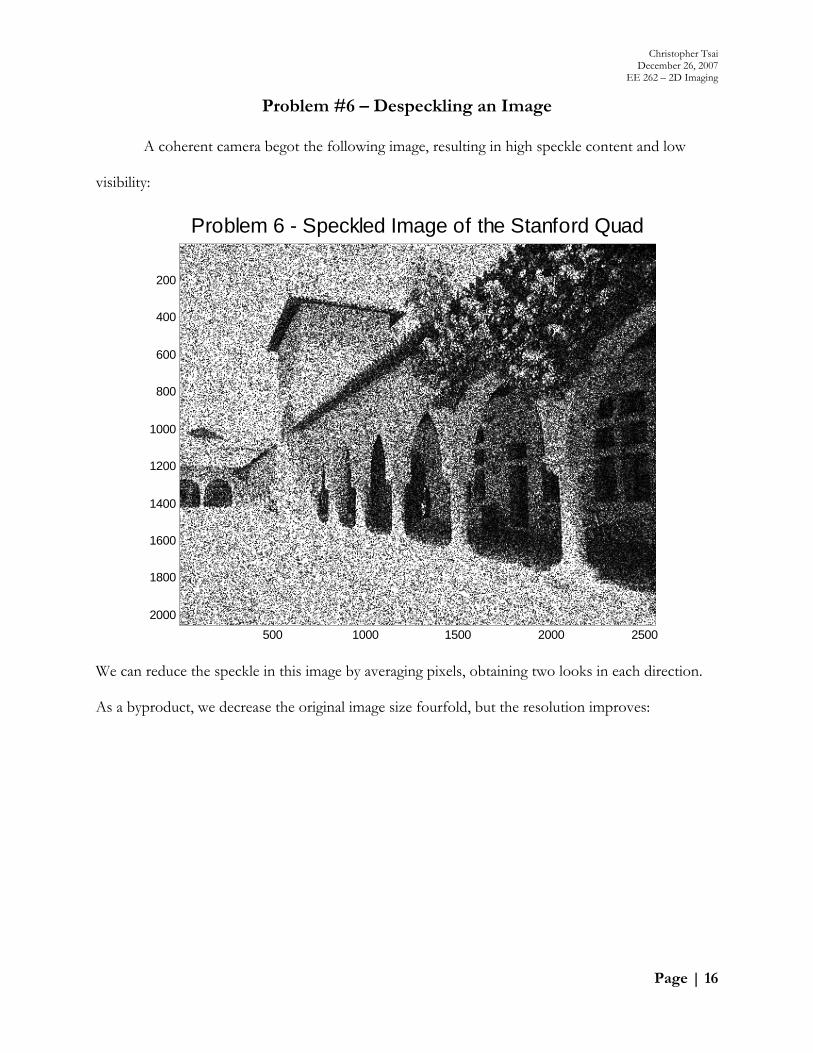
Problem #6 – Despeckling an Image
A coherent camera begot the following image, resulting in high speckle content and low
visibility:
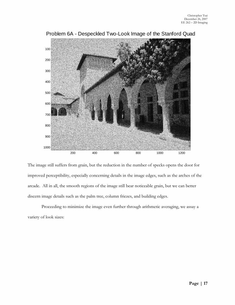
We can reduce the speckle in this image by averaging pixels, obtaining two looks in each direction.
As a byproduct, we decrease the original image size fourfold, but the resolution improves:
Problem 6 - Speckled Image of the Stanford Quad
500 1000 1500 2000 2500
200
400
600
800
1000
1200
1400
1600
1800
2000
Christopher Tsai December 26, 2007
EE 262 – 2D Imaging
Page | 17
The image still suffers from grain, but the reduction in the number of specks opens the door for
improved perceptibility, especially concerning details in the image edges, such as the arches of the
arcade. All in all, the smooth regions of the image still bear noticeable grain, but we can better
discern image details such as the palm tree, column friezes, and building edges.
Proceeding to minimize the image even further through arithmetic averaging, we assay a
variety of look sizes:
Problem 6A - Despeckled Two-Look Image of the Stanford Quad
200 400 600 800 1000 1200
100
200
300
400
500
600
700
800
900
1000
Christopher Tsai December 26, 2007
EE 262 – 2D Imaging
Page | 18
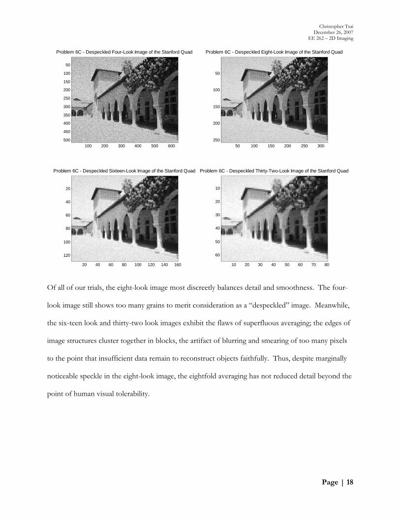
Of all of our trials, the eight-look image most discreetly balances detail and smoothness. The four-
look image still shows too many grains to merit consideration as a “despeckled” image. Meanwhile,
the six-teen look and thirty-two look images exhibit the flaws of superfluous averaging; the edges of
image structures cluster together in blocks, the artifact of blurring and smearing of too many pixels
to the point that insufficient data remain to reconstruct objects faithfully. Thus, despite marginally
noticeable speckle in the eight-look image, the eightfold averaging has not reduced detail beyond the
point of human visual tolerability.
Problem 6C - Despeckled Four-Look Image of the Stanford Quad
100 200 300 400 500 600
50
100
150
200
250
300
350
400
450
500
Problem 6C - Despeckled Eight-Look Image of the Stanford Quad
50 100 150 200 250 300
50
100
150
200
250
Problem 6C - Despeckled Sixteen-Look Image of the Stanford Quad
20 40 60 80 100 120 140 160
20
40
60
80
100
120
Problem 6C - Despeckled Thirty-Two-Look Image of the Stanford Quad
10 20 30 40 50 60 70 80
10
20
30
40
50
60