Economics 623 J.R.WalkerPage 1

Problem Set 2: Answers

The problem set came from Michael A. Trick, Senior Associate Dean, Education and Pro-fessor Tepper School of Business, Carnegie Mellon University. Professor Trick’s url containingthe tutorial on dynamic programming is: http://mat.gsia.cmu.edu/classes/dynamic/dynamic.html. What follows are pages directly from Trick’s web page.

Next: A second example Up: A Tutorial on Dynamic Previous: Contents

First ExampleLet's begin with a simple capital budgeting problem. A corporation has $5 million to allocate to its threeplants for possible expansion. Each plant has submitted a number of proposals on how it intends to spendthe money. Each proposal gives the cost of the expansion (c) and the total revenue expected (r). Thefollowing table gives the proposals generated:

Table 1: Investment Possibilities

Each plant will only be permitted to enact one of its proposals. The goal is to maximize the firm's revenuesresulting from the allocation of the $5 million. We will assume that any of the $5 million we don't spend islost (you can work out how a more reasonable assumption will change the problem as an exercise).

A straightforward way to solve this is to try all possibilities and choose the best. In this case, there are only ways of allocating the money. Many of these are infeasible (for instance, proposals 3, 4,

and 1 for the three plants costs $6 million). Other proposals are feasible, but very poor (like proposals 1, 1,and 2, which is feasible but returns only $4 million).

Here are some disadvantages of total enumeration:

1. For larger problems the enumeration of all possible solutions may not be computationally feasible.2. Infeasible combinations cannot be detected a priori, leading to inefficiency.3. Information about previously investigated combinations is not used to eliminate inferior, or

infeasible, combinations.

Note also that this problem cannot be formulated as a linear program, for the revenues returned are notlinear functions.

One method of calculating the solution is as follows:

Let's break the problem into three stages: each stage represents the money allocated to a single plant. Sostage 1 represents the money allocated to plant 1, stage 2 the money to plant 2, and stage 3 the money toplant 3. We will artificially place an ordering on the stages, saying that we will first allocate to plant 1, thenplant 2, then plant 3.

Each stage is divided into states. A state encompasses the information required to go from one stage to thenext. In this case the states for stages 1, 2, and 3 are

{0,1,2,3,4,5}: the amount of money spent on plant 1, represented as ,{0,1,2,3,4,5}: the amount of money spent on plants 1 and 2 ( ), and{5}: the amount of money spent on plants 1, 2, and 3 ( ).

Unlike linear programming, the do not represent decision variables: they are simply representations of ageneric state in the stage.

Associated with each state is a revenue. Note that to make a decision at stage 3, it is only necessary toknow how much was spent on plants 1 and 2, not how it was spent. Also notice that we will want to be5.

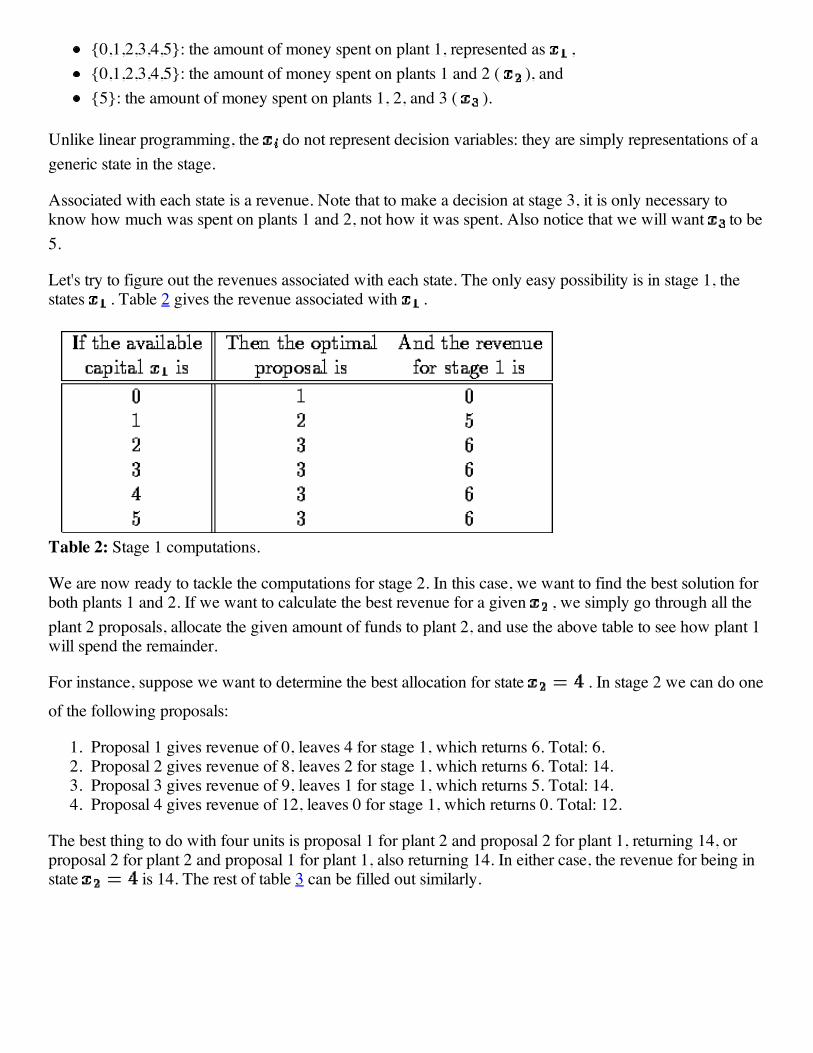
Let's try to figure out the revenues associated with each state. The only easy possibility is in stage 1, thestates . Table 2 gives the revenue associated with .

Table 2: Stage 1 computations.

We are now ready to tackle the computations for stage 2. In this case, we want to find the best solution forboth plants 1 and 2. If we want to calculate the best revenue for a given , we simply go through all theplant 2 proposals, allocate the given amount of funds to plant 2, and use the above table to see how plant 1will spend the remainder.

For instance, suppose we want to determine the best allocation for state . In stage 2 we can do one

of the following proposals:

1. Proposal 1 gives revenue of 0, leaves 4 for stage 1, which returns 6. Total: 6.2. Proposal 2 gives revenue of 8, leaves 2 for stage 1, which returns 6. Total: 14.3. Proposal 3 gives revenue of 9, leaves 1 for stage 1, which returns 5. Total: 14.4. Proposal 4 gives revenue of 12, leaves 0 for stage 1, which returns 0. Total: 12.

The best thing to do with four units is proposal 1 for plant 2 and proposal 2 for plant 1, returning 14, orproposal 2 for plant 2 and proposal 1 for plant 1, also returning 14. In either case, the revenue for being instate is 14. The rest of table 3 can be filled out similarly.

Table 3: Stage 2 computations.

We can now go on to stage 3. The only value we are interested in is . Once again, we go throughall the proposals for this stage, determine the amount of money remaining and use Table 3 to decide thevalue for the previous stages. So here we can do the following at plant 3:

Proposal 1 gives revenue 0, leaves 5. Previous stages give 17. Total: 17.Proposal 2 gives revenue 4, leaves 4. Previous stages give 14. Total: 18.

Therefore, the optimal solution is to implement proposal 2 at plant 3, proposal 2 or 3 at plant 2, andproposal 3 or 2 (respectively) at plant 1. This gives a revenue of 18.

If you study this procedure, you will find that the calculations are done recursively. Stage 2 calculations arebased on stage 1, stage 3 only on stage 2. Indeed, given you are at a state, all future decisions are madeindependent of how you got to the state. This is the principle of optimality and all of dynamicprogramming rests on this assumption.

We can sum up these calculations in the following formulas:

Denote by the revenue for proposal at stage j, and by the corresponding cost.

Let be the revenue of state in stage j. Then we have the following calculations

and

All we were doing with the above calculations was determining these functions.

The computations were carried out in a forward procedure. It was also possible to calculate things from the``last'' stage back to the first stage. We could define

= amount allocated to stages 1, 2, and 3, = amount allocated to stages 2 and 3, and = amount allocated to stage 3.

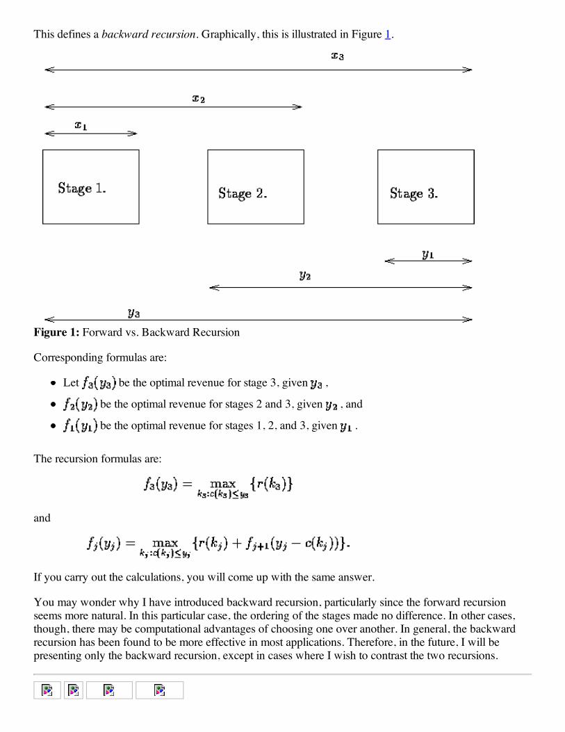
This defines a backward recursion. Graphically, this is illustrated in Figure 1.

Figure 1: Forward vs. Backward Recursion

Corresponding formulas are:

Let be the optimal revenue for stage 3, given ,

be the optimal revenue for stages 2 and 3, given , and

be the optimal revenue for stages 1, 2, and 3, given .

The recursion formulas are:

and

If you carry out the calculations, you will come up with the same answer.

You may wonder why I have introduced backward recursion, particularly since the forward recursionseems more natural. In this particular case, the ordering of the stages made no difference. In other cases,though, there may be computational advantages of choosing one over another. In general, the backwardrecursion has been found to be more effective in most applications. Therefore, in the future, I will bepresenting only the backward recursion, except in cases where I wish to contrast the two recursions.

2/25/12 A second example

1/3mat.gsia.cmu.edu/classes/dynamic/node3.html#SECTION00030000000000000000

Next: Common Characteristics Up: A Tutorial on Dynamic Previous: First Example

A second exampleDynamic programming may look somewhat familiar. Both our shortest path algorithm and our method forCPM project scheduling have a lot in common with it.

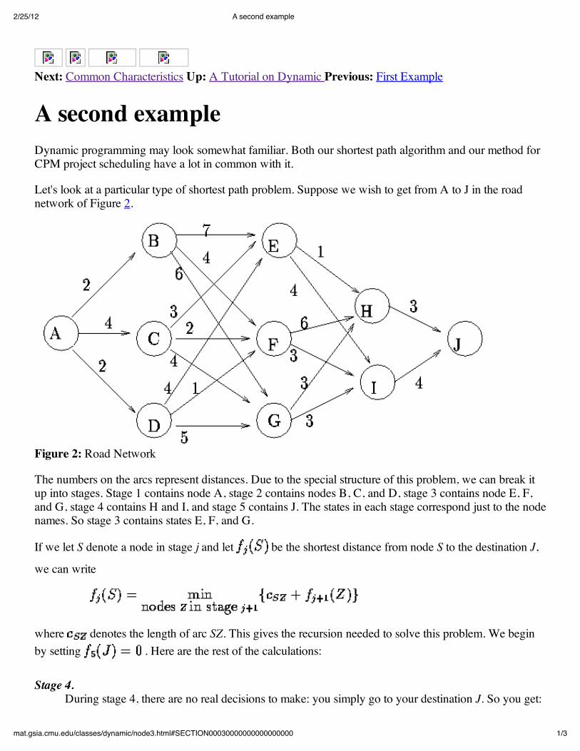
Let's look at a particular type of shortest path problem. Suppose we wish to get from A to J in the roadnetwork of Figure 2.

Figure 2: Road Network

The numbers on the arcs represent distances. Due to the special structure of this problem, we can break itup into stages. Stage 1 contains node A, stage 2 contains nodes B, C, and D, stage 3 contains node E, F,and G, stage 4 contains H and I, and stage 5 contains J. The states in each stage correspond just to the nodenames. So stage 3 contains states E, F, and G.

If we let S denote a node in stage j and let be the shortest distance from node S to the destination J,

we can write

where denotes the length of arc SZ. This gives the recursion needed to solve this problem. We beginby setting . Here are the rest of the calculations:

Stage 4.During stage 4, there are no real decisions to make: you simply go to your destination J. So you get:

2/25/12 A second example

2/3mat.gsia.cmu.edu/classes/dynamic/node3.html#SECTION00030000000000000000

by going to J,

by going to J.

Stage 3.Here there are more choices. Here's how to calculate . From F you can either go to H or I.

The immediate cost of going to H is 6. The following cost is . The total is 9. The

immediate cost of going to I is 3. The following cost is for a total of 7. Therefore, if you

are ever at F, the best thing to do is to go to I. The total cost is 7, so .

The next table gives all the calculations:

You now continue working back through the stages one by one, each time completely computing a stagebefore continuing to the preceding one. The results are:

Stage 2.

Stage 1.

Next: Common Characteristics Up: A Tutorial on Dynamic Previous: First Example

Michael A. Trick

Next: The Knapsack Problem. Up: A Tutorial on Dynamic Previous: A second example

Common CharacteristicsThere are a number of characteristics that are common to these two problems and to all dynamicprogramming problems. These are:

1. The problem can be divided into stages with a decision required at each stage.

In the capital budgeting problem the stages were the allocations to a single plant. The decision washow much to spend. In the shortest path problem, they were defined by the structure of the graph.The decision was were to go next.

2. Each stage has a number of states associated with it.

The states for the capital budgeting problem corresponded to the amount spent at that point in time.The states for the shortest path problem was the node reached.

3. The decision at one stage transforms one state into a state in the next stage.

The decision of how much to spend gave a total amount spent for the next stage. The decision ofwhere to go next defined where you arrived in the next stage.

4. Given the current state, the optimal decision for each of the remaining states does not depend on theprevious states or decisions.

In the budgeting problem, it is not necessary to know how the money was spent in previous stages,only how much was spent. In the path problem, it was not necessary to know how you got to anode, only that you did.

5. There exists a recursive relationship that identifies the optimal decision for stage j, given that stagej+1 has already been solved.

6. The final stage must be solvable by itself.

The last two properties are tied up in the recursive relationships given above.

The big skill in dynamic programming, and the art involved, is to take a problem and determine stages andstates so that all of the above hold. If you can, then the recursive relationship makes finding the valuesrelatively easy. Because of the difficulty in identifying stages and states, we will do a fair number ofexamples.

Next: The Knapsack Problem. Up: A Tutorial on Dynamic Previous: A second example

Michael A. Trick Sun Jun 14 13:05:46 EDT 1998

Next: An Alternative Formulation Up: A Tutorial on Dynamic Previous: Common Characteristics

The Knapsack Problem.The knapsack problem is a particular type of integer program with just one constraint. Each item that cango into the knapsack has a size and a benefit. The knapsack has a certain capacity. What should go into theknapsack so as to maximize the total benefit? As an example, suppose we have three items as shown inTable 4, and suppose the capacity of the knapsack is 5.

Table 4: Knapsack Items

The stages represent the items: we have three stages j=1,2,3. The state at stage j represents the totalweight of items j and all following items in the knapsack. The decision at stage j is how many items j toplace in the knapsack. Call this value .

This leads to the following recursive formulas: Let be the value of using units of capacity for

items j and following. Let represent the largest integer less than or equal to a.

Michael A. Trick Sun Jun 14 13:05:46 EDT 1998

Next: Equipment Replacement Up: A Tutorial on Dynamic Previous: The Knapsack Problem.

An Alternative FormulationThere is another formulation for the knapsack problem. This illustrates how arbitrary our definitions ofstages, states, and decisions are. It also points out that there is some flexibility on the rules for dynamicprogramming. Our definitions required a decision at a stage to take us to the next stage (which we wouldalready have calculated through backwards recursion). In fact, it could take us to any stage we havealready calculated. This gives us a bit more flexibility in our calculations.

The recursion I am about to present is a forward recursion. For a knapsack problem, let the stages beindexed by w, the weight filled. The decision is to determine the last item added to bring the weight to w.There is just one state per stage. Let g(w) be the maximum benefit that can be gained from a w poundknapsack. Continuing to use and as the weight and benefit, respectively, for item j, the following

relates g(w) to previously calculated g values:

Intuitively, to fill a w pound knapsack, we must end off by adding some item. If we add item j, we end upwith a knapsack of size to fill. To illustrate on the above example:

g(0) = 0g(1) = 30 add item 3.

add item 1.

add item 1 or 3.

add item

1. add item

1 or 3.

This gives a maximum of 160, which is gained by adding 2 of item 1 and 1 of item 3.

Michael A. Trick Sun Jun 14 13:05:46 EDT 1998

Next: The Traveling Salesperson Problem Up: A Tutorial on Dynamic Previous: An AlternativeFormulation

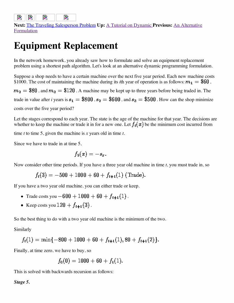
Equipment ReplacementIn the network homework, you already saw how to formulate and solve an equipment replacementproblem using a shortest path algorithm. Let's look at an alternative dynamic programming formulation.

Suppose a shop needs to have a certain machine over the next five year period. Each new machine costs$1000. The cost of maintaining the machine during its ith year of operation is as follows: ,

, and . A machine may be kept up to three years before being traded in. The

trade in value after i years is , , and . How can the shop minimize

costs over the five year period?

Let the stages correspond to each year. The state is the age of the machine for that year. The decisions arewhether to keep the machine or trade it in for a new one. Let be the minimum cost incurred from

time t to time 5, given the machine is x years old in time t.

Since we have to trade in at time 5,

Now consider other time periods. If you have a three year old machine in time t, you must trade in, so

If you have a two year old machine, you can either trade or keep.

Trade costs you .

Keep costs you .

So the best thing to do with a two year old machine is the minimum of the two.

Similarly

Finally, at time zero, we have to buy, so

This is solved with backwards recursion as follows:

Stage 5.

Stage 4.

Stage 3.

Stage 2.

Stage 1.

Stage 0.

So the cost is 1280, and one solution is to trade in years 1 and 2. There are other optimal solutions.

Next: The Traveling Salesperson Problem Up: A Tutorial on Dynamic Previous: An Alternative

Next: Nonadditive Recursions Up: A Tutorial on Dynamic Previous: Equipment Replacement

The Traveling Salesperson ProblemWe have seen that we can solve one type of integer programming (the knapsack problem) with dynamicprogramming. Let's try another.

The traveling salesperson problem is to visit a number of cities in the minimum distance. For instance, apolitician begins in New York and has to visit Miami, Dallas, and Chicago before returning to New York.How can she minimize the distance traveled? The distances are as in Table 5.

Table 5: TSP example problem.

The real problem in solving this is to define the stages, states, and decisions. One natural choice is to letstage t represent visiting t cities, and let the decision be where to go next. That leaves us with states.Imagine we chose the city we are in to be the state. We could not make the decision where to go next, forwe do not know where we have gone before. Instead, the state has to include information about all thecities visited, plus the city we ended up in. So a state is represented by a pair (i,S) where S is the set of tcities already visited and i is the last city visited (so i must be in S). This turns out to be enough to get arecursion.

The stage 3 calculations are

For other stages, the recursion is

You can continue with these calculations. One important aspect of this problem is the so called curse ofdimensionality. The state space here is so large that it becomes impossible to solve even moderate sizeproblems. For instance, suppose there are 20 cities. The number of states in the 10th stage is more than amillion. For 30 cities, the number of states in the 15th stage is more than a billion. And for 100 cities, thenumber of states at the 50th stage is more than 5,000,000,000,000,000,000,000,000,000,000. This is notthe sort of problem that will go away as computers get better.

Next: Stochastic Dynamic Programming Up: A Tutorial on Dynamic Previous: The Traveling SalespersonProblem

Nonadditive RecursionsNot every recursion must be additive. Here is one example where we multiply to get the recursion.

A student is currently taking three courses. It is important that he not fail all of them. If the probability of failingFrench is , the probability of failing English is , and the probability of failing Statistics is , then theprobability of failing all of them is . He has left himself with four hours to study. How should he minimizehis probability of failing all his courses? The following gives the probability of failing each course given he studiesfor a certain number of hours on that subject, as shown in Table 6.

Table 6: Student failure probabilities.

(What kind of student is this?) We let stage 1 correspond to studying French, stage 2 for English, and stage 3 forStatistics. The state will correspond to the number of hours studying for that stage and all following stages. Let

be the probability of failing t and all following courses, assuming x hours are available. Denote the entries

in the above table as , the probability of failing course t given k hours are spent on it.

The final stage is easy:

The recursion is as follows:

We can now solve this recursion:

Stage 3.

There is one major difference between stochastic dynamic programs and deterministic dynamic programs:in the latter, the complete decision path is known. In a stochastic dynamic program, the actual decision pathwill depend on the way the random aspects play out. Because of this, ``solving'' a stochastic dynamicprogram involves giving a decision rule for every possible state, not just along an optimal path.

Next: ``Linear'' decision making Up: Stochastic Dynamic Programming Previous: Uncertain Payoffs

Michael A. Trick Sun Jun 14 13:05:46 EDT 1998

Next: Uncertain Payoffs Up: A Tutorial on Dynamic Previous: Nonadditive Recursions

Stochastic Dynamic ProgrammingIn deterministic dynamic programming, given a state and a decision, both the immediate payoff and nextstate are known. If we know either of these only as a probability function, then we have a stochasticdynamic program. The basic ideas of determining stages, states, decisions, and recursive formulae stillhold: they simply take on a slightly different form.

Uncertain PayoffsUncertain States``Linear'' decision making

Michael A. Trick Sun Jun 14 13:05:46 EDT 1998

Next: Uncertain States Up: Stochastic Dynamic Programming Previous: Stochastic DynamicProgramming

Uncertain PayoffsConsider a supermarket chain that has purchased 6 gallons of milk from a local dairy. The chain mustallocate the 6 gallons to its three stores. If a store sells a gallon of milk, then the chain receives revenue of$2. Any unsold milk is worth just $.50. Unfortunately, the demand for milk is uncertain, and is given in thefollowing table:

The goal of the chain is to maximize the expected revenue from these 6 gallons. (This is not the onlypossible objective, but a reasonable one.)

Note that this is quite similar to some of our previous resource allocation problems: the only difference isthat the revenue is not known for certain. We can, however, determine an expected revenue for eachallocation of milk to a store. For instance, the value of allocating 2 gallons to store 1 is:

We can do this for all allocations to get the following values:

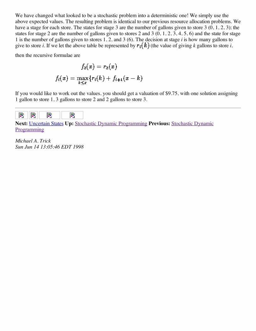
We have changed what looked to be a stochastic problem into a deterministic one! We simply use theabove expected values. The resulting problem is identical to our previous resource allocation problems. Wehave a stage for each store. The states for stage 3 are the number of gallons given to store 3 (0, 1, 2, 3); thestates for stage 2 are the number of gallons given to stores 2 and 3 (0, 1, 2, 3, 4, 5, 6) and the state for stage1 is the number of gallons given to stores 1, 2, and 3 (6). The decision at stage i is how many gallons togive to store i. If we let the above table be represented by (the value of giving k gallons to store i,

then the recursive formulae are

If you would like to work out the values, you should get a valuation of $9.75, with one solution assigning1 gallon to store 1, 3 gallons to store 2 and 2 gallons to store 3.

Next: Uncertain States Up: Stochastic Dynamic Programming Previous: Stochastic DynamicProgramming

Michael A. Trick Sun Jun 14 13:05:46 EDT 1998

Next: ``Linear'' decision making Up: Stochastic Dynamic Programming Previous: Uncertain Payoffs

Uncertain StatesA more interesting use of uncertainty occurs when the state that results from a decision is uncertain. Forexample, consider the following coin tossing game: a coin will be tossed 4 times. Before each toss, you canwager $0, $1, or $2 (provided you have sufficient funds). You begin with $1, and your objective is tomaximize the probability you have $5 at the end. of the coin tosses.

We can formulate this as a dynamic program as follows: create a stage for the decision point before eachflip of the coin, and a ``final'' stage, representing the result of the final coin flip. There is a state in eachstage for each possible amount you can have. For stage 1, the only state is ``1'', for each of the others, youcan set it to ``0,1,2,3,4,5'' (of course, some of these states are not possible, but there is no sense in worryingtoo much about that). Now, if we are in stage i and bet k and we have x dollars, then with probability .5,we will have x-k dollars, and with probability .5 we will have x+k dollars next period. Let be the

probability of ending up with at least $5 given we have $x before the ith coin flip.

This gives us the following recursion:

Note that the next state is not known for certain, but is a probabilistic mixing of states. We can still easilydetermine from , and from and so on back to .

Another example comes from the pricing of stock options. Suppose we have the option to buy Netscapestock at $150. We can exercise this option anytime in the next 10 days (american option, rather than aeuropean option that could only be exercised 10 days from now). The current price of Netscape is $140.We have a model of Netscape stock movement that predicts the following: on each day, the stock will goup by $2 with probability .4, stay the same with probability .1 and go down by $2 with probability .4. Notethat the overall trend is downward (probably conterfactual, of course). The value of the option if weexercise it at price x is x-150 (we will only exercise at prices above 150).

We can formulate this as a stochastic dynamic program as follows: we will have stage i for each day i, justbefore the exercise or keep decision. The state for each stage will be the stock price of Netscape on thatday. Let be the expected value of the option on day i given that the stock price is x. Then, the

optimal decision is given by:

and

Given the size of this problem, it is clear that we should use a spreadsheet to do the calculations.

There is one major difference between stochastic dynamic programs and deterministic dynamic programs:in the latter, the complete decision path is known. In a stochastic dynamic program, the actual decision pathwill depend on the way the random aspects play out. Because of this, ``solving'' a stochastic dynamicprogram involves giving a decision rule for every possible state, not just along an optimal path.

Next: ``Linear'' decision making Up: Stochastic Dynamic Programming Previous: Uncertain Payoffs

Michael A. Trick Sun Jun 14 13:05:46 EDT 1998

Next: About this document Up: Stochastic Dynamic Programming Previous: Uncertain States

``Linear'' decision making. Many decision problems (and some of the most frustrating ones), involve choosing one out of a numberof choices where future choices are uncertain. For example, when getting (or not getting!) a series of joboffers, you may have to make a decision on a job before knowing if another job is going to be offered toyou. Here is a simplification of these types of problems:

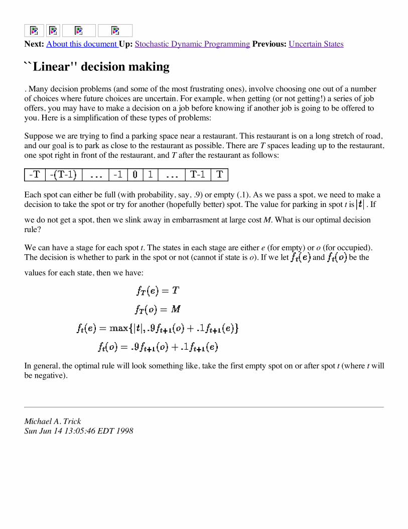
Suppose we are trying to find a parking space near a restaurant. This restaurant is on a long stretch of road,and our goal is to park as close to the restaurant as possible. There are T spaces leading up to the restaurant,one spot right in front of the restaurant, and T after the restaurant as follows:

Each spot can either be full (with probability, say, .9) or empty (.1). As we pass a spot, we need to make adecision to take the spot or try for another (hopefully better) spot. The value for parking in spot t is . If

we do not get a spot, then we slink away in embarrasment at large cost M. What is our optimal decisionrule?

We can have a stage for each spot t. The states in each stage are either e (for empty) or o (for occupied).The decision is whether to park in the spot or not (cannot if state is o). If we let and be the

values for each state, then we have:

In general, the optimal rule will look something like, take the first empty spot on or after spot t (where t willbe negative).

Michael A. Trick Sun Jun 14 13:05:46 EDT 1998