Case Study 4: Piezoelectric Rectangular Multilayer Plate

PROBLEM - 3D Two Layer Plate, PZT4, 10mm x 5mm x 1mm Layer Thickness, Inter-digital Electrode

GOAL

Evaluate the operation of a composite piezoelectric rectangular plate having electrodes in the top, middle, and bottom large surfaces and two different polarization layers in the thickness mode. The introduction of Inter-Digital electrodes with the analysis of Internal Stress Distribution. The size of the plate is 10mm x 5mm x H=1mm (2X). The piezoelectric material PZT4.

Figure C4.1. Composite Piezoelectric Plate with Inter-digital Electrodes.

L = 10 mm

W = 5 mm

H = 2 mm (1mm + 1mm)

Material: PZT4

Top , Middle, and Bottom Electrodes

Thickness Polarization

GEOMETRY/DRAWING

1. Start GiD or

Although applicable for most versions of GiD and Atila this example will use GiD 11 and Atila 3.0.27. This example assumes that the user has done Cases 1-3 and is somewhat familiar with the GiD/Atila environment. Assuming familiarity this case uses the Icon Toolbars in the illustrations as the first option. The Drop Down Menus will produce the same results. To review the icon/menu correlation please refer to Case Study 1.

2. Create the 3D Model

2.1 Creating the rectangle and surface

Click ( ) ( ) Enter first corner point 0,0 Enter Enter second corner point 10,5 Enter . The Rectangle is created as shown in Figure C4.2.

Figure C4.2. Rectangle created

2.2 Dividing the surface The surface will be divided to create the end sections of the plate. The divisions are at (1,0) and 9,0) resulting in 1 mm wide end sections.

Click Geometry Edit Divide Surfaces Near Point Select Surface Choose Nurbs Sense (U) Enter Coordinates Enter. Repeat until all divisions are made.The sequence for dividing the surfaces is shown in Figure C4.3. through C4.7.

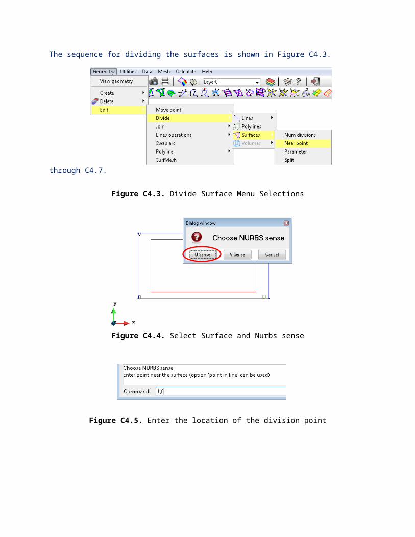
Figure C4.3. Divide Surface Menu Selections

Figure C4.4. Select Surface and Nurbs sense

Figure C4.5. Enter the location of the division point

Note: the division point is the location coordinates, ie 1,0.

Figure C4.6. Resultant divided surface

2.3 Create the second divisionSelect larger surface and enter division point.

Figure C4.7. Second Division point and Results after second division

2.4 Create Volumes using Copy

Click ( ) Copy Panel appears (See figure C.4.8 left panel)Select Surfaces Translate Enter first point (X,Y,Z) 0,0,0 Enter second point (X,Y,Z 0,0,1.0 Do Extrude Volumes Maintain Layers Multiple Copies (2) Select Select Surfaces to Translate Finish. The results are seen in right panel of Figure C4.8.

Copy Panel Volumes Created

Figure C4.8. Volumes created

MATERIALS AND CONDITIONS

Access Note: The material, conditions, and data menus are interconnected and other panels can be

accessed from within each panel by clicking the ( ) icon. The fly-out menu will allow selection of any of the other items pertaining to conditions and materials. When selected the panel will change to the new panel selected. See Figure C4.9. for an example of the sequence.

Figure C4.9. Access between Panels

3. Material Assignment3.1 Assignment of piezoelectric material

Click ( ) Select PZT4 Assign Volumes Select volumes Finish or ESC

3.2 Confirm assignment of materialClick Draw Colors as illustrated in Figure C4.10. Finish to quit.

1 32

Figure C4.10. Confirm Material Assignment

4. Boundary Conditions Assignment

Click ( ) the Boundary Conditions Panel appears. (Can also access by clicking in the Piezoelectric material panel and select Conditions as illustrated in Figure C4.8.)

4.1 Polarization Assignment

Click ( ) Polarization-Cartesian Local Axes Define Enter name of local axis (P1) OK Choose definition mode 3 Points XZ Place Cursor in Command Line Enter Center (0,0,0) Enter Select Join Positive X Direction (1,0,0) Enter Select Join Positive Z Direction (0,0,1) Enter Select Join Assign Select Top Volume Finish.

Click Local Axes Define Enter name of local axis (P2) OK Choose definition mode 3 Points XZ Place Cursor in Command Line Enter Center (0,0,0) Enter Select Join Positive X Direction (1,0,0) Enter Select Join Positive Z Direction (0,0,-1) Enter Select Join Assign Select Bottom Volumes Finish.

Note: To avoid the need to select “Join” after each coordinate use a value that does not fall on an already existing point, for example the X axis could be 2,0,0.

4.2 Confirm Polarization AssignmentClick Draw Colors as illustrated in Figure C4.11. left panel Finish or ESC to quit Click Draw Polarization Include Local Axes as illustrated in Figure C4.11. right panel. Click Finish or ESC to quit.

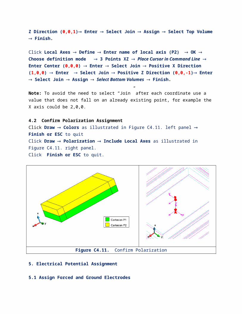
Figure C4.11. Confirm Polarization

5. Electrical Potential Assignment

5.1 Assign Forced and Ground Electrodes

Click Select Electrical Potential Forced Amplitude enter 1.0 Assign Select Center Right small Surface and Center large Surface Finish or ESC as shown in Figure C4.12 Top panel.Confirm Forced Electrode AssignmentClick Draw Colors to confirm assignment as illustrated in Figure C4.12. bottom panelClick Finish or ESC to quit.

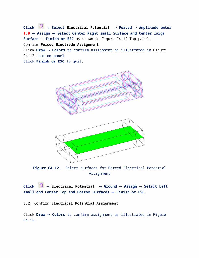
Figure C4.12. Select surfaces for Forced Electrical Potential Assignment

Click Electrical Potential Ground Assign Select Left small and Center Top and Bottom Surfaces Finish or ESC.

5.2 Confirm Electrical Potential Assignment

Click Draw Colors to confirm assignment as illustrated in Figure C4.13. Click Finish or ESC to quit

Figure C4.13. Confirm Electrical Potential Assignment

MESH

Defining the Mesh

Note: The GiD default setting for mesh is Normal using Tetrahedral elements, however, this example will use Hexahedral elements. This change can be made in the Preferences Panel or selected through the Mesh menu.

7. Meshing the ModelClick Mesh Structured Volumes Assign number of cells Select VolumesThe Enter value window appears.Enter number of cells to assign to lines Enter (2) Assign Select short lines ESCEnter number of cells to assign to lines (16) Assign Select long lines ESC ESC to quit

Set the element typeClick Mesh Element type Hexahedra Select Volumes ESC. See Figure C4.14.

Figure C4.14. Select Element type

Mesh the partClick Control + G Mesh generation panel appears Accept default (OK) Dialog panel appears View Mesh the results appear as seen in Figure C4.15

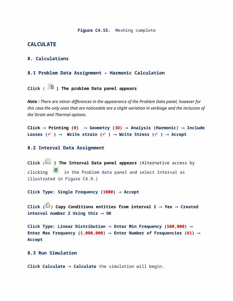
Figure C4.15. Meshing complete

CALCULATE

8. Calculations

8.1 Problem Data Assignment – Harmonic Calculation

Click ( ) The problem Data panel appears

Note : There are minor differences in the appearance of the Problem Data panel, however for this case the only ones that are noticeable are a slight variation in verbiage and the inclusion of the Strain and Thermal options. Click Printing (0) Geometry (3D) Analysis (Harmonic) Include Losses ( ) Write strain ( ) Write Stress ( ) Accept

8.2 Interval Data Assignment

Click ( ) The Interval Data panel appears (Alternative access by clicking in the Problem data panel and select Interval as illustrated in Figure C4.9.)

Click Type: Single Frequency (1000) Accept

Click ( ) Copy Conditions entities from interval 1 Yes Created interval number 2 Using this OK

Click Type: Linear Distribution Enter Min Frequency (500,000) Enter Max Frequency (1,000,000) Enter Number of Frequencies (61) Accept

8.3 Run Simulation

Click Calculate Calculate the simulation will begin.

The Process info panel appears when the simulation is completeClick Postprocess to load the simulation results.

To enter the post-process mode if OK is selected or after exiting the post-process mode Click ( ). This will open the last simulation run.

Results

10. Post Process - Graphs

10.1 Admittance Graph

Click ( ) the Admittance & Impedance Results panel appears Select Admittance: Magnitude View Graph to view the admittance graph. See graph in Figure C4.16.

Note: Click ( ) to toggle between the graph and model view.

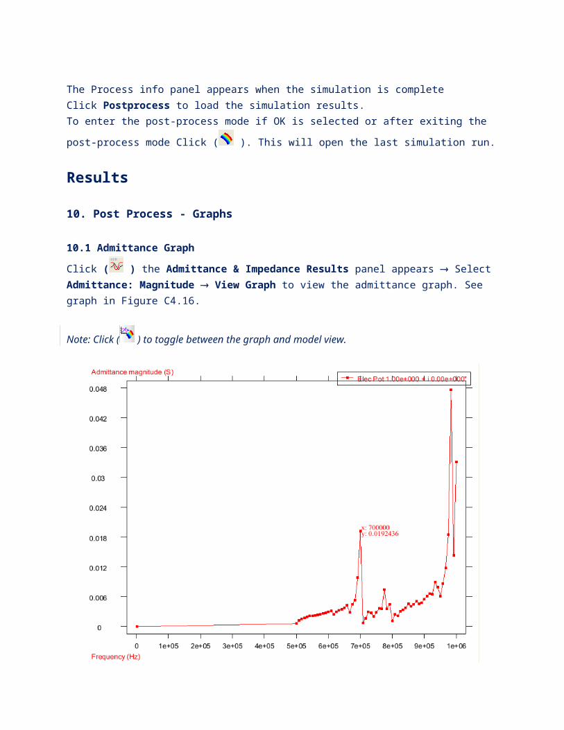
Figure C4.16. Admittance Graph

11. Animations

11.1 Animation of Stress

The Siii stress at the resonance frequency of 70,000 Hz as illustrated in Figure C4.17.

Figure C4.17. Animation of Stress Siii @ 70,000 Hz

11.2 Animation of Electrical Potential

The electrical potential at the frequency of 1000 Hz as illustrated in Figure C4.18.

Figure C4.18. Electrical Potential at 1000 Hz