Probing Interactions in Fixed and Multilevel Regression...

Probing Interactions in Fixed andMultilevel Regression: Inferential and

Graphical Techniques

Daniel J. Bauer and Patrick J. CurranUniversity of North Carolina at Chapel

Many important research hypotheses concern conditional relations in which the ef-fect of one predictor varies with the value of another. Such relations are commonlyevaluated as multiplicative interactions and can be tested in both fixed- and ran-dom-effects regression. Often, these interactive effects must be further probed tofully explicate the nature of the conditional relation. The most common method forprobing interactions is to test simple slopes at specific levels of the predictors. Amore general method is the Johnson-Neyman (J-N) technique. This technique is notwidely used, however, because it is currently limited to categorical by continuous in-teractions in fixed-effects regression and has yet to be extended to the broader classof random-effects regression models. The goal of our article is to generalize the J-Ntechnique to allow for tests of a variety of interactions that arise in both fixed- andrandom-effects regression. We review existing methods for probing interactions, ex-plicate the analytic expressions needed to expand these tests to a wider set of condi-tions, and demonstrate the advantages of the J-N technique relative to simple slopeswith three empirical examples.

Substantive theories within psychology, education and many other disciplines inthe social sciences are replete with instances in which the effect of one predictor onthe outcome is hypothesized to vary as a function of a second predictor. We will re-fer to the first of these predictors as the focal predictor and the second as the mod-erator, although this distinction is strictly theoretical. Hypotheses concerning

MULTIVARIATE BEHAVIORAL RESEARCH, 40(3), 373–400Copyright © 2005, Lawrence Erlbaum Associates, Inc.

This work was funded in part by fellowship DA06062 awarded to the first author and grantDA13148 awarded to the second author. We would like to thank R. J. Wirth and the members of theCarolina Structural Equations Modeling Group for their valuable input throughout this project.

Correspondence concerning this article should be addressed to Daniel J. Bauer, L.L. ThurstonePsychometric Laboratory, Department of Psychology, University of North Carolina, Chapel Hill,NC 27599–3270. E-mail: [email protected]

moderated relationships can be evaluated in the standard fixed-effects regressionmodel (e.g., Cohen, Cohen, West, & Aiken, 2003), or they can manifest in morecomplicated ways in the multilevel (or random effects) regression model (e.g.,Raudenbush & Bryk, 2002). Regardless of the analytic approach, testing theunique contribution of the product term net the lower-order main effects providesan omnibus test of the interaction effect (Baron & Kenny, 1986; Cohen, 1978).More detailed information on the nature of the moderated relationship must thenbe obtained through the use of techniques for probing the interaction term (e.g.,Aiken & West, 1991).

For the standard fixed-effects regression model, the most popular method forprobing interactions is the “pick-a-point” approach (Rogosa, 1980). This approachinvolves plotting and testing the conditional effect of the focal predictor at desig-nated levels of the moderating variable (e.g., high, medium, and low), where theseconditional effect estimates are commonly referred to as “simple slopes” (Aiken &West, 1991; Jaccard & Turrisi, 2003). Although widely used in fixed-effects regres-sion, the consideration of simple slopes in random-effects regression has been lim-ited. While Hox (2002, pp. 58–63) recommended the plotting of simple slopes to aidin the interpretation of interactions in multilevel models, to our knowledge this ap-proach has only been used in a small number of empirical applications and almost al-ways as a descriptive rather than inferential device (e.g., Bryk & Raudenbush, 1987,p.154;Hussong,2003;Willett,Singer&Martin,1998,p.423;Yip&Fuligni,2002).

While the pick-a-point approach is informative and easy to use, typically only asmall number of specific values of the moderator are selected to evaluate the condi-tional effect of the focal predictor on the outcome. These values are often selectedsomewhat arbitrarily (Rogosa, 1980), and may even reside outside of the range ofthe sample data (e.g., one standard deviation above the mean of a skewed predic-tor). Interest may instead center on how the conditional effect of the focal predictorchanges across the entire range of a continuous moderating variable, rather thanjust at a few values.

One such instance is when a grouping variable and continuous variable interactin an ANCOVA or linear regression model. In the presence of such an interaction,the group means cannot be compared by simply adjusting for differences on thecontinuous covariate. An alternative approach is to evaluate the group mean differ-ence at each level of the covariate with the goal of determining when the groupmean differences are and are not statistically different. The J-N technique was de-veloped for this purpose (Johnson & Fay, 1950; Johnson & Neyman, 1936) and in-volves the use of two closely related procedures for evaluating conditional effects,the computation of regions of significance and confidence bands (Huitema, 1980).Whereas regions of significance define the levels of the covariate for which thegroup mean difference is significant, confidence bands convey the precision withwhich the group mean difference is estimated at each level of the covariate.

374 BAUER AND CURRAN

There are two key advantages of the J-N technique. First, regions of signifi-cance provide an inferential test for any possible simple slope of the focal predictorvariable. Second, the confidence bands graphically depict the precision of estima-tion of the effect of the focal predictor over the full range of the moderator, provid-ing a range of likely values for the conditional effect that narrows or widens de-pending on the selected level of the moderator. The point where the confidencebands are narrowest, also known as the center of accuracy, represents the value ofthe moderator at which we have the most confidence estimating the conditional ef-fect of the focal predictor on the outcome.

Despite these distinct advantages of the J-N technique, the use of regions of sig-nificance and confidence bands for evaluating interactions remains extremely lim-ited. One possible reason for this is that the J-N technique has not been generalizedto settings other than the traditional dichotomous by continuous interaction in theANCOVA model, even in such recent treatments as Cohen et al. (2003) andJaccard and Turrisi (2003). For instance, to our knowledge there are no publishedapplications in which this technique has been applied to evaluate continuous bycontinuous interactions in standard regression models. Further, aside from somepreliminary developments by ourselves (Bauer, Curran, & Bollen, 2001; Curran,Bauer, & Willoughby, 2004, in press) and Miyazaki (2002), we are aware of noprior work that has extended these methods in a general way to the random-effectsor multilevel regression model.1 Our goal is to make these extensions here. We firstpresent our expansion of the J-N technique for the more familiar fixed-effects re-gression model, then extend the use of this technique to the multilevel regressionmodel involving random effects. Empirical examples are provided throughout toillustrate the use of these procedures.

PROBING INTERACTIONSIN FIXED-EFFECTS REGRESSION

A simple fixed-effects regression model involving two predictors and their interac-tion can be expressed in scalar notation as

yi = �0 + �1x1i + �2x2i + �3x1ix2i + �i. (1)

The coefficient �3 represents the interaction, defined as the effect of the x1x2 prod-uct variable on the dependent variable y over and above the additive main effects ofthe predictors x1 and x2 (�1 and �2, respectively). The residuals � represent the por-tion of variability in y that is unexplained by the predictors.

PROBING INTERACTIONS 375

1Since the writing of this manuscript, related work on this topic has been published by Tate (2004).

For this model, we can define the prediction equation to be

where the expected value of y conditioned upon specific values of x1 and x2 is de-noted Finally, we can rearrange Equation 2 to highlight how the effect ofone predictor varies as a function of the other. Treating x1 as the focal predictor andx2 as the moderator, we have

explicating that the y on x1 regression line varies as a function of x2. We can thendesignate the simple intercept and simple slope of this conditional relationship as�0 and �1, respectively:

�0 = �0 + �2x2, (4)

�1 = �1 + �3x2. (5)

One important fact that Equations 4 and 5 highlight is that, in the presence of aproduct interaction, the intercept and main effects of the regression model arescale-dependent. For instance, Equation 5 shows that the main effect of the focalpredictor (�1) is the effect where the moderator is zero (x2 = 0). Because zero is of-ten outside the logical range of the moderator, it is recommended to mean center orstandardize predictors involved in interactions so that the main effects representthe effects of each predictor at the mean level of the other (see Jaccard, Turrisi, &Wan, 1990, and Aiken & West, 1991, who also discuss computational advantagesof mean centering predictors). While this aids in the interpretation of the main ef-fect, we will typically also want to assess the effect of the focal predictor at levelsof the moderator other than zero to more fully explore the nature of the interaction.The pick-a-point and J-N techniques provide alternative methods for accomplish-ing this goal. For both approaches, the key is to obtain an estimate and standard er-ror for a parameter (e.g., �1) that is a linear composite of other parameters (e.g., �1

and �3). We now show how to compute these values for the simple slope of the fo-cal predictor (�1), as it is usually this value that is of most interest, though similarprocedures could also be applied to the simple intercept (�0).


1 2| , .y x x�

� � � �1 2| , 0 2 2 1 3 2 1, (3)y x x x x x� � � � ��

1 2| , 0 1 1 2 2 3 1 2 , (2)y x x x x x x� � � � ��

Estimating Conditional Effects in Fixed-Effects Regression

In the general case, the fixed-effects regression model may be written as

y = X� + �, (6)

where y is an n × 1 criterion vector, X is the n × p design matrix for p-predictor vari-ables (including a column vector of 1’s to define the intercept), � is a p × 1 vector offixed regression parameters relating each predictor to the criterion, and � is an n × 1vector of random residuals. The residuals are assumed to be homoscedastic andnormally distributed [i.e., ]. In the specific case of the two-predictorinteraction model given in Equation 1, the matrix X would simply consist of a col-umn of 1’s, a column of observed values for x1, a column of observed values for x2,and a column of values for the product of x1 and x2.

From a frequentist perspective, the parameter estimates of the model may beviewed as random variables characterized by a joint sampling distribution. Givensufficiently large samples, this sampling distribution will obtain a multivariate nor-mal form. Conditional effect estimates may then be viewed as weighted linearcomposites of these random normal variates (Aiken & West, 1991, pp. 25–26;Morrison, 1990, p. 83):

where a is a p × 1 column vector containing the a1, a2, …, ap fixed weights used toform the composite. The variance of the conditional effect is estimated as

where is the sample estimate of the asymptotic covariance matrix ofthe regression coefficient estimates given by the usual formula

The standard error of the estimate is then simply the square root of the variance es-timate obtained from Equation 8.


� �2, nN �0 I� �

1 0 2 1 1 ˆˆ ˆ ˆ ˆ , (7)p pa a a� � � � � �� a ��

VAR VAR ACOV� � �ˆ ˆ ˆ , ( )�( )= ′( )= ′ ( )a a a� � 8

ACOV� �̂( )

ACOV n� ˆ ˆ

ˆ . ( )

�( )= ′( )

= ′( )

− −

−

X I X

X X

�

�

2 1 1

2 19

For our simple two-predictor example the vector of regression coefficient esti-mates is

Thus, to obtain a point estimate and standard error for �1 as defined in Equation 5,we would set

and solve Equations 7 and 8 to obtain the point estimate and variance of the simpleslope where

Equations 12 and 13 represent the two fundamental pieces of information that willbe manipulated to probe the interaction effect.

We next briefly review the testing of simple slopes using the pick-a-point ap-proach, and then proceed to detail how the J-N technique can be applied to morefully evaluate conditional effects resulting from the interaction of categorical orcontinuous predictors.

The Pick-a-Point Approach: Tests of Simple Slopes

A traditional test of simple slopes using the pick-a-point technique consists ofcomputing conditional effect estimates �� and their variances using Equa-tions 7 and 8 for several fixed values of the moderating variable (e.g., 0 and 1 if themoderator is binary, or high, medium, and low values if it is continuous). A test of asimple slope is then obtained by forming the critical ratio of the conditional effectestimate to its standard error at a specified level of the moderator:

Cohen et al. (2003) and Jaccard and Turrisi (2003) have also suggested construct-ing confidence intervals for simple slope estimates rather than relying exclusivelyon null hypothesis tests, a point that we will return to and reinforce shortly. In addi-tion, a graphical depiction of the interaction may also be obtained by computing


1 1 3 2ˆ ˆ ˆ , (12)x� � ��

VAR VAR x COV x VAR� � � �ˆ ˆ ˆ , ˆ ˆ . ( )� � � � �1 1 2 1 3 22

32 13( )= ( )+ ( )+ ( )

� � �ˆVAR �

tVAR

=( )

ˆ

ˆ. ( )

/

�

�� 1 214

� �20 1 0 , (11)x� �a

� �0 1 2 3ˆ ˆ ˆ ˆ ˆ . (10)� � � ��

both simple intercepts and simple slopes for each of several levels of the moderatorand then plotting the simple regression lines given by these estimates.

While this approach has been an extremely useful method for probing interac-tions inmanyareasofapplied research, it is typically limited to theevaluationofcon-ditional effects at only a small number of values of the moderator. There is not a sys-tematic way to examine the magnitude of the conditional effects, nor their precision,across the entire range of the moderator, information that is provided by the moregeneral J-N technique.For this reason,wenowturn toa furtherexplicationof the J-Ntechnique in both fixed-effects and random-effects regression.

The J-N Technique

We distinguish between two related aspects of the J-N technique: The computationof regions of significance and the plotting of confidence bands for the conditionaleffect. To our knowledge, this presentation is the first to expand the use of the J-Ntechnique beyond the traditional ANCOVA framework. In our view, this expansionhas been impeded by the traditional formulation of the J-N technique from sepa-rate within-group linear regressions of the outcome on the covariate (see Aiken &West, 1991, pp. 134–136; Jaccard & Turrisi, 2003, pp. 81–82). Extension of thetechnique to continuous by continuous interactions is then nonobvious, given thelack of discretely defined groups. However, as has been shown elsewhere (Hunka,1995; Rogosa, 1980, 1981) the traditional J-N technique can be embedded in ageneral linear model involving an interaction between the grouping variable andcontinuous covariate. It then becomes a relatively simple matter to consider use ofthe J-N technique for interactions between continuous variables as well. We thusmotivate the J-N technique from the standpoint of the general fixed-effects regres-sion model. This presentation has the added benefit of explicating the analytical re-lation between the J-N technique and the pick-a-point approach which in turn fa-cilitates our ultimate goal of extending the J-N technique to a broad class ofrandom-effects regression models.

Regions of significance. The computation of regions of significance is analternative to the pick-a-point approach that indicates over what range of the mod-erator the effect of the focal predictor is significantly positive, nonsignificant, orsignificantly negative. To compute regions of significance, we reverse the un-known quantity in the critical ratio in Equation 14. Specifically, rather than solvefor the t value that corresponds to the simple slope at the designated level of themoderator, we select a critical value tcrit (i.e., ±1.96 for large samples) and solve forthe values of the moderator that return that critical value:


± =( )

tVAR

critˆ

ˆ. ( )

/

�

�� 1 215

Manipulation of this equation yields

For interactions involving two predictors, the two roots of the moderator that sat-isfy this equality can be solved by the quadratic formula. These roots demarcatethe boundaries of the regions of significance, indicating the points on the scale ofthe moderator at which the effect of the focal predictor passes from significance tononsignificance at the selected alpha-level.

For example, let us again consider the conditional effect of x1 in the simple twopredictor model in Equation 1. Substituting in the expressions in Equations 12 and13 into Equation 16 and collecting terms, we have

where

The values of x2 satisfying this equality can then be obtained via the quadratic for-mula

The two values (or roots) of x2 that are returned by this formula demarcate theboundaries of the regions of significance.2 Note that this holds regardless of thedistribution of the moderator. The moderator may thus be categorical or continu-


ax bx c22

2 0 17+ + = , ( )

a t VARcrit= ( )−23 3

2 18� ˆ ˆ , ( )� �

b t COVcrit= ( )−

2 192

1 3 1 3� ˆ , ˆ ˆ ˆ , ( )� � � �

c t VARcrit= ( )−21 1

2 20� ˆ ˆ . ( )� �

2Sometimes the conditional effect of the focal predictor will be nonsignificant at any given level ofthe moderator despite a significant test of the product interaction term. Mathematically, this will resultin there being no real roots to Equation 21 (i.e., the roots will be imaginary numbers). The opposite canalso occur, where regions of significance and nonsignficance can be identified despite the lack of a sig-nificant interaction term. Rogosa (1980, 1981) provides a useful discussion of these scenarios.

2

24

. (21)2

b b acx

a

� � ��

t VARcrit2 2 0 16� ˆ ˆ . ( )� �( )− =

ous, making the traditional application of the J-N technique in the ANCOVAmodel a special case of Equation 16.

Confidence bands. One common feature of tests of simple slopes and re-gions of significance is that both procedures are based on traditional null hypothe-sis testing. However, the usefulness of this approach to statistical inference hasbeen questioned repeatedly over the decades, culminating in the APA task force re-port emphasizing that confidence intervals are much more informative than nullhypothesis tests (Wilkinson & the Task Force on Statistical Inference, 1999). Simi-larly, as we now show, confidence bands provide more information than null hy-pothesis tests of simple slopes and regions of significance.

The standard formula for a confidence interval (CI) is

where represents a given point estimate. In most cases we are interested in a sin-gle effect estimate and so simply compute the confidence interval for this estimate.However, in the case of conditional effects, both the effect estimate and its standarderror vary as a function of the moderating variable. As such, we cannot plot justone confidence interval; instead we must plot the confidence interval over the fullrange of the moderating variable, and these are known as confidence bands(Rogosa, 1980, 1981). The general formula for the confidence bands (CB) is then

To continue with our simple two predictor model, if we were interested in com-puting confidence bands for the effect of the focal predictor x1 as a function of themoderator x2, we would substitute in the specific conditional effect estimate of x1

and its variance as given in Equations 12 and 13:

As is the case with standard confidence intervals, these confidence bands conveythe same information as null hypothesis tests of simple slopes and/or regions ofsignificance. Specifically, the points where the confidence bands cross zero are theboundaries of the regions of significance (also indicating which simple slopes aresignificant and which are not).


CI t VARcrit= ± ( ) ˆ ˆ , ( )/

� �� 1 222

CB t VARcritˆ/

ˆ ˆ . ( )� � �= ± ( ) � 1 223

CB x t VAR x COV x VARcritˆ ˆ ˆ ˆ ˆ , ˆ ˆ� � � � � �1 1 3 2 1 2 1 3 222= +( ) ± ( )+ ( )+� � � ��3

1 224( )

/. ( )

�̂

Additionally, the confidence bands graphically convey our certainty in the con-ditional effect estimates and how that certainty changes as we progress across therange of the moderating variable. The confidence bands are narrowest at the centerof accuracy. This point can be obtained by differentiating the variance function forthe conditional effect estimate with respect to the moderating variable and settingthe resulting derivative equal to zero

Solving for values of the moderator, here denoted xm, that satisfy this equality willproduce candidate points for the center of accuracy. For our simple examplemodel, manipulation of Equation 25 shows that the center of accuracy is the valueof x2 given by the formula

More complicated variance functions may have more than one candidate point forthe center of accuracy, requiring that these points be compared to determine theone yielding the smallest variance. Typically, the center of accuracy will be in themiddle of the scale of the moderator, with decreasing precision evident at the endsof the scale.

Multiple Testing: Nonsimultaneous VersusSimultaneous Inference

The regions and bands explicated above, as well as the pick-a-point proceduredescribed before them, are all predicated on the use of an alpha-level that is onlyvalid for a single test. The inferences they afford must thus be regarded asnonsimultaneous. As such, the Type I error rates of these techniques are onlyfully accurate for a single selected value of the moderator and the error rate willotherwise accumulate as additional values of the moderator are considered. Ifone wished to simultaneously evaluate the effect of the focal predictor at a smallnumber of values of the moderator (e.g., high, medium, and low, as in tests ofsimple slopes), a family-wise alpha-level could be obtained by using, for in-stance, the Bonferroni approach (Neter, Kutner, Nachtsheim, & Wasserman,1996, pp. 157–158). This approach could similarly be applied to the regions andconfidence bands of the J-N technique so that inferences would be valid for aspecific number of values of the moderator. If, with the J-N technique, valid in-


xCOV

VAR2

1 3

3

26=− ( )

( )

�

�ˆ , ˆ

ˆ. ( )

� �

�

d

dxVAR

m

� ˆ . ( )�( )= 0 25

ferences are sought for all values of the moderator simultaneously, then one caninstead use the critical values derived by Potthoff (1964) to compute simulta-neous regions of significance and confidence bands. In the simple case of themodel considered above, the critical t value in Equations 15 through 24 wouldbe replaced by [2Fcrit(2, N – p)]1/2 (see also Rogosa, 1980, 1981, and Serber,1977). If the number of comparisons to be made is not small, this approach willgenerally be more powerful than using the Bonferroni approach and has the fur-ther advantage of yielding an accurate Type I error rate for all possible compari-sons (Neter et al., 1996, pp. 157–158).

Despite these advantages, the simultaneous critical value of Potthoff (1964)will necessarily yield narrower regions of significance and broader confidencebands than the nonsimultaneous critical value, sometimes so much so that the re-sults may be of little practical use, as noted by Potthoff himself. As a possible rem-edy to the problem, Potthoff suggested using a higher alpha level with the simulta-neous approach. Others have suggested alternative forms for the confidence bandsthat are valid only over specific (observed) intervals of the moderating variable,rather than over the entire real line (Aitken, 1973; Gafarian, 1964). Unless other-wise noted, here we focus specifically on the nonsimultaneous version of the J-Ntechnique for the principal reasons that this facilitates an understanding of the rela-tion between the pick-a-point and J-N procedures, no consensus has yet emergedon the best method for constructing simultaneous regions and confidence bands,and the simultaneous approach is often impractical. Mindful of the error rate accu-mulation problem of the nonsimultaneous approach, however, we view the result-ing regions and bands as primarily of heuristic value.

Empirical Example: The Relation Between Child MathAbility, Delinquency, and Hyperactivity

To demonstrate the application of the J-N technique to probe a continuous by con-tinuous interaction in a fixed-effects regression model, we considered a sample ofN = 956 children drawn from the 1990 assessment of the Children of the NationalLongitudinal Survey of Youth (NLSY). Children ranged in age from 59 to 156months (mean age of 100 months), ranged in grade from kindergarten to sixthgrade (third grade was the median), 52% were female, and 55% of mothers re-ported their child to be of minority status (self identified to be non-Caucasian). Themotivating substantive question related to the prediction of math ability as a func-tion of the joint influence of antisocial and hyperactive behavior. It was hypothe-sized that there would be a negative relation between child antisocial behavior andmath ability, and that this effect would be potentiated by the additional presence ofchild hyperactive behavior.

The regression model used to evaluate this hypothesis was identical to Equa-tion 1, with the exception that age, grade, sex, and minority status were entered


as additional covariates. Here, y is mathematics ability, measured as the propor-tion of 84 items correctly endorsed on the math subsection of the Peabody Indi-vidual Achievement Test (y = 37.65, sd = 15.77, range = 5.95 – 82.14), x1 is acontinuous measure of antisocial behavior as reported by the child’s mother (x1

= 1.34, sdx1= 1.34, range = 0 – 6), x2 is a continuous measure of hyperactive

behavior as reported by the child’s mother (x 2 = 1.94, sdx 2= 1.54, range = 0 –

5), and larger values of these variables reflect higher levels of child antisocialand hyperactive behavior. We mean-centered all predictors (including the co-variates) prior to fitting the model using ordinary least squares estimation.3

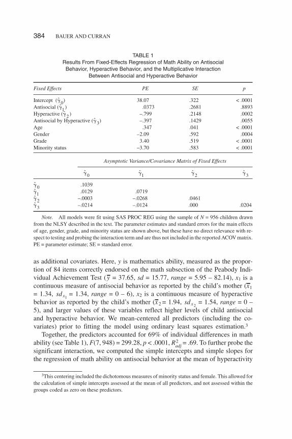
Together, the predictors accounted for 69% of individual differences in mathability (see Table 1), F(7, 948) = 299.28, p < .0001, Radj

2 = .69. To further probe thesignificant interaction, we computed the simple intercepts and simple slopes forthe regression of math ability on antisocial behavior at the mean of hyperactivity


3This centering included the dichotomous measures of minority status and female. This allowed forthe calculation of simple intercepts assessed at the mean of all predictors, and not assessed within thegroups coded as zero on these predictors.

TABLE 1Results From Fixed-Effects Regression of Math Ability on Antisocial

Behavior, Hyperactive Behavior, and the Multiplicative InteractionBetween Antisocial and Hyperactive Behavior

Fixed Effects PE SE p

Intercept (��0) 38.07 .322 < .0001Antisocial (��1 ) .0373 .2681 .8893Hyperactive (��2 ) –.799 .2148 .0002Antisocial by Hyperactive (��3) –.397 .1429 .0055Age .347 .041 < .0001Gender –2.09 .592 .0004Grade 3.40 .519 < .0001Minority status –3.70 .583 < .0001

Asymptotic Variance/Covariance Matrix of Fixed Effects

��0��1

��2��3

��0 .1039��1 .0129 .0719��2 –.0003 –.0268 .0461��3 –.0214 –.0124 .000 .0204

Note. All models were fit using SAS PROC REG using the sample of N = 956 children drawnfrom the NLSY described in the text. The parameter estimates and standard errors for the main effectsof age, gender, grade, and minority status are shown above, but these have no direct relevance with re-spect to testing and probing the interaction term and are thus not included in the reported ACOV matrix.PE = parameter estimate; SE = standard error.

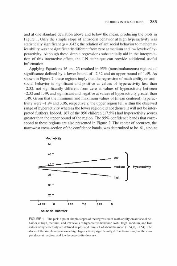
and at one standard deviation above and below the mean, producing the plots inFigure 1. Only the simple slope of antisocial behavior at high hyperactivity wasstatistically significant (p = .045); the relation of antisocial behavior to mathemat-ics ability was not significantly different from zero at medium and low levels of hy-peractivity. Although these simple regressions substantially aid in the interpreta-tion of this interactive effect, the J-N technique can provide additional usefulinformation.

Applying Equations 16 and 23 resulted in 95% (nonsimultaneous) regions ofsignificance defined by a lower bound of –2.32 and an upper bound of 1.49. Asshown in Figure 2, these regions imply that the regression of math ability on anti-social behavior is significant and positive at values of hyperactivity less than–2.32, not significantly different from zero at values of hyperactivity between–2.32 and 1.49, and significant and negative at values of hyperactivity greater than1.49. Given that the minimum and maximum values of (mean centered) hyperac-tivity were –1.94 and 3.06, respectively, the upper region fell within the observedrange of hyperactivity whereas the lower region did not (hence it will not be inter-preted further). Indeed, 167 of the 956 children (17.5%) had hyperactivity scoresgreater than the upper bound of the region. The 95% confidence bands that corre-spond to these regions are also presented in Figure 2. The center of accuracy, thenarrowest cross-section of the confidence bands, was determined to be .61, a point


FIGURE 1 The pick-a-point simple slopes of the regression of math ability on antisocial be-havior at high, medium, and low levels of hyperactive behavior. Note. High, medium, and lowvalues of hyperactivity are defined as plus and minus 1 sd about the mean (1.54, 0, −1.54). Theslope of the simple regression at high hyperactivity significantly differs from zero, but the sim-ple slope at medium and low hyperactivity does not.

where the effect of antisocial behavior is nonsignificant. For contrast, the simulta-neous regions of significance were also calculated (not shown in Figure 2), withobtained roots of –5.52 and 2.18. The lower root is well outside the observed rangeof the data, and only 7% of the children’s hyperactivity scores were observedabove the upper root. The smaller region of significance with the simultaneous ap-proach is a natural consequence of trade-off between simultaneous inference andpower, but in this case the region includes such a small portion of the sample that itis of relatively little practical use.

In summary, the J-N technique provides much additional information relativeto the pick-a-point approach. Indeed, the testing of specific simple slopes is alsoprovided by the J-N technique (e.g., the simple slopes of the high, medium andlow regression lines plotted in Figure 1, and their confidence intervals, simplyreflect three specific points on the abscissa in Figure 2). In addition, these re-gions convey that the effect of antisocial behavior on mathematics ability is sig-nificant at any given level of hyperactivity higher than 1.49 units above the meanand that we have the most confidence estimating this effect for hyperactivity lev-els slightly above the mean. All of these results, and the corresponding plots, canbe calculated using a suite of freely available javascript programs accessible athttp://www.quantpsy.org that implement the formulas presented in this paper.Table 1 provides all the necessary information for the interested reader to repli-cate our results using this program. We now turn to the extension of the J-Ntechnique to a broad class of random-effects regression models.


FIGURE 2 J-N regions of significance and confidence bands for the conditional relation be-tween math ability and antisocial behavior as a function of hyperactivity. Note. Dashed verticallines reflect regions of significance (−2.32, 1.49) and the dark horizontal line with diamonds in-dicates the range of child hyperactivity observed in the sample data (−1.94, 3.06). The intersec-tion of values of hyperactivity equal to −1.54, 0, and 1.54 with effect of antisocial behavior cor-respond to the three simple slopes presented in Figure 1.

PROBING INTERACTIONSIN MULTILEVEL REGRESSION

Unlike the standard fixed-effects regression models, interactions can be mani-fested in a variety of ways in multilevel models. They may occur within a givenlevel of the model (e.g., an interaction between two lower-level or two up-per-level variables) or between levels of the model (e.g., an interaction betweena lower-level variable and an upper-level variable). Moreover, some interactionswill involve predictors whose main effects are random, or even the interactionmay be a random effect, whereas in other cases these effects will be fixed. Themost common of these scenarios is the cross-level interaction with a randommain effect for the lowest level predictor. We use this case to show how the J-Ntechnique can be extended and applied to multilevel models, but of course theseprocedures directly apply to the other types of interactions that can arise in mul-tilevel models as well.

A cross-level interaction arises when the random coefficient of a lower levelpredictor is itself predicted by an upper level predictor. In the simplest case, thelevel-1 model can be written as

yij = �0j + �1jx1ij + �ij, (27)

where yij is the outcome variable for individual i in group j, x1ij is the single predic-tor for individual i in group j, �0j and �1j are the intercept and slope of the regres-sion of y on x1 within group j, respectively, and �ij is the random residual for indi-vidual i within group j. Given that the intercept and slope coefficients varyrandomly over groups, these can be conceived as random variables to be predictedby one or more group-level covariates. In the case of a single group-level covariate,the level-2 model can be written as

�0j = �00 + �01w1j + u0j, (28)

�1j = �10 + �11w1j + u1j, (29)

where w1j represents the single predictor for group j, �00 and �10 are the fixed inter-cepts of the regression of �0j and �1j on w1j, and �01 and �11 represent the fixedslopes of the regression of �0j and �1j on w1j, and u0j and u1j reflect the residualvariability in the level-1 intercepts and slopes net the prediction by w1j.

Although there is only a single main effect in the level-1 equation and a singlemain effect in each level-2 equation, the cross-level interaction effect is apparent in


the reduced-form equation, obtained by substituting Equations 28 and 29 intoEquation 27 and grouping fixed and random components:

yij = (�00 + �01w1j + �10x1ij + �11x1ijw1j) + (u0j + u1jx1ij + �ij). (30)

This equation illustrates that the main effect regression of the random slopes onw1 (�11) is expressed as a cross-level interaction between w1 and x1 in the re-duced form equation (i.e., �11w1jx1ij). Given the formulation of the level-1 andlevel-2 models, we would traditionally view w1 as the moderator of the effect ofx1. However, as always, the conditional effects in the model are symmetrical,and in the reduced-form model we can see that there is no restriction on whichvariable is to be considered the focal predictor or moderator.

To consider the conditional nature of the effects of each predictor in greater de-tail, we first write the prediction equation for the model. Taking the expectation ofEquation 30 over both individuals and groups yields the prediction equation

The simple slope for the regression of y on x1 as a function of w1 is then

Similarly, given the symmetry of the interaction, the simple slope of the regressionof y on w1 can be written as a function of x1, or

As for the standard regression model, the challenge is then again to obtain an esti-mate and standard error for a linear composite. Given that this linear compositeconsists entirely of fixed effects, we will see that this task is accomplished in muchthe same way for the multilevel regression model as it was for the standard regres-sion model.

Estimating Conditional Effects in Multilevel Models

More formally, the reduced form of the linear multilevel model can be expressed as

yj = Xj� + Zjuj + �j, (34)

where yj is the nj × 1 response vector for group j = 1, 2, …, J, Xj is the nj × p designmatrix for the p × 1 vector of fixed effects � (where p includes a column vector of


1 10 11 1. (32)x w� � ��

1 01 11 1. (33)w x� � ��

1 1| , 00 10 1 01 1 11 1 1. (31)y x w x w x w� � � � ��

1’s for the intercept), Zj is the nj × q design matrix for the q × 1 vector of random ef-fects uj, and �j is the nj × 1 vector of residuals (Laird & Ware, 1982). Importantly, itis assumed that the random effects and residuals are independent of one anotherand are multivariate normally distributed as

Although not requisite, the form of the covariance matrix of the random effects T istypically unrestricted and the residuals are often constrained to be homoscedasticand independent (i.e., �� j jn� 2I ). Without loss of generality we follow theseconventions here, although all of our developments apply to any structure of T and�� j (assuming these are properly identified).

As we demonstrated earlier, once we move to the prediction equation by takingexpectations over both individuals and groups, we are left with conditional effectsthat are linear composites of fixed coefficients only. Thus, the estimated condi-tional effect of x at a given level of w (or vice versa) can be computed from Equa-tion 7 just as in the case of the standard regression model. Similarly, application ofEquation 8 will yield the variance of this estimate. Where these computations dif-fer from the standard fixed-effects case is that the asymptotic covariance matrix ofthe fixed-effects estimates no longer has the simple form of Equation 9, and in-stead is estimated as

where �Vj is the model-implied covariance matrix for yj, estimated as

Equation 37 would simplify to Equation 9 if �T (or equivalently Z) were a null ma-trix, that is, in the absence of random effects.

For example, consider the cross-level interaction in the multilevel regressionmodel in Equation 30. Arranging the vector of fixed effect parameter estimates as


2ˆ ˆ ˆ . (38)jj j j n�� V Z TZ I

ACOV j j jj

J� ˆ ˆ , ( )�( )= ′

−

=

−

∑X V X1

1

1

37

� �00 01 10 11ˆ ˆ ˆ ˆ ˆ , (39)� � � ��

� �, , (35)j Nu 0 T�

� �, . (36)jj N �0� ��

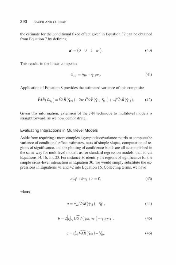
the estimate for the conditional fixed effect given in Equation 32 can be obtainedfrom Equation 7 by defining

This results in the linear composite

Application of Equation 8 provides the estimated variance of this composite

Given this information, extension of the J-N technique to multilevel models isstraightforward, as we now demonstrate.

Evaluating Interactions in Multilevel Models

Aside from requiring a more complex asymptotic covariance matrix to compute thevariance of conditional effect estimates, tests of simple slopes, computation of re-gions of significance, and the plotting of confidence bands are all accomplished inthe same way for multilevel models as for standard regression models, that is, viaEquations 14, 16, and 23. For instance, to identify the regions of significance for thesimple cross-level interaction in Equation 30, we would simply substitute the ex-pressions in Equations 41 and 42 into Equation 16. Collecting terms, we have

where


211 0, (43)aw bw c� � �

a t VARcrit= ( )−211 11

2 44� ˆ ˆ , ( )� �

VAR VAR w COV w VARx� � � �ˆ ˆ ˆ , ˆ ˆ . (� � � � �1 10 1 10 11 1

2112 42( )= ( )+ ( )+ ( ) ))

b t COVcrit= ( )−

2 452

10 11 10 11� ˆ , ˆ ˆ ˆ , ( )� � � �

1 10 11 1ˆ ˆ ˆ . (41)x w� � ��

� �10 0 1 . (40)w� �a

c t VARcrit= ( )−210 10

2 46� ˆ ˆ . ( )� �

As before, the two values of w1 that satisfy this equality represent the boundaries ofthe regions of significance and can be obtained via the quadratic formula. Note thatthis again holds regardless of whether the moderator is categorical or continuous.

Similarly, substituting the expressions in Equations 41 and 42 into Equation 23,we see that the confidence bands are defined by the function

The center of accuracy can be determined by solving Equation 25, in this case re-sulting in the formula

The value of w1 satisfying this equality is the value at which the conditional effectof x1 is estimated with greatest certainty.

Despite the apparent ease with which the J-N technique generalizes to multi-level models, it is important to note one key complication. Under standard assump-tions, the test statistics obtained from a standard regression model are exactly t-dis-tributed with n – p degrees of freedom. Unfortunately, the same is not typically truefor a multilevel model; even under standard assumptions, the test statistics for thefixed effects are typically only approximately t-distributed (Kacker & Harville,1984; Schaalje, McBride, & Fellingham, 2002). By implication, while exact testsof simple slopes, boundaries to the regions of significance, and width of the confi-dence bands can be obtained in the absence of random effects, when random ef-fects are present the same computations provide only approximately valid infer-ences. As such, appropriate caution should be exercised in the interpretation of theresults of these procedures in multilevel models. In particular, one should not placetoo much emphasis on the specific values obtained for the boundaries to the re-gions of significance, as these boundaries would likely change if another methodfor approximating the test distribution was selected (e.g., an alternative method fordetermining degrees of freedom). For cross-level interactions, we expect that theresults will be most sensitive to this choice when there is a small sample size at theupper level of the model.

Similarly, while the distinction between nonsimultaneous and simultaneousversions of the J-N technique also arises in the multilevel model, the test statistic isnot as easily derived as in the fixed-effects regression model. Specifically,Miyazaki (2002) argued that a critical F would be inappropriate given the morecomplex error structure of the multilevel model and has instead advocated the use


wCOV

VAR1

10 11

11

48=− ( )

( )

�

�ˆ , ˆ

ˆ. ( )

� �

�

CB w

t VAR w COV w

x

crit

ˆ ˆ ˆ

ˆ ˆ , ˆ

� � �

� � �

1 10 11 1

10 1 10 11 12

= +( )±

( )+ ( )+� � 2211

1 247VAR� ˆ . ( )

/�( )

of a Wald test that is chi-square distributed when the number of groups J is large.Given that many applications of multilevel models involve a relatively small num-ber of groups, the asymptotic nature of this test may provide a serious impedimentto the simultaneous approach as outlined by Miyazaki. For this reason, and thoseadumbrated previously, we continue to use the nonsimultaneous version of the J-Ntechnique here. However, whether one prefers a nonsimultaneous or simultaneousapproach, it is fair to say that more study is needed to determine the optimalmethod for testing conditional effects in small samples so as to obtain accurate andstable estimates of the regions of significance and confidence bands.4

In summary, the principal difficulties associated with applying the J-N tech-nique to multilevel models are no different than those that impact any multilevelmodeling analysis, regardless of the presence of within-level or cross-level interac-tive effects. Specifically, the asymptotic covariance matrix of the fixed effects musttake account of the additional variance components in the model and the test distri-bution for the fixed effects estimates is only approximately known so tests are typi-cally inexact. Neither of these issues detracts from our ability to apply the J-N tech-nique to evaluate conditional effects, and much interpretive information is to begained from their use, as we now demonstrate with an empirical application.

EMPIRICAL EXAMPLE

Todemonstrate theuseofJ-Nregionsandbands inpractice,weconsidereddata fromthe High School and Beyond (HSB) study that was described in detail by Rauden-bush and Bryk (2002) and Singer (1998). These data consist of a total sample of7,185 students who are nested within 160 schools. Between 14 to 67 students wereassessed from each school, with a median of number of 47 students assessed. Theoutcome of interest is a child-level measure of math achievement (y = 12.75, sd =6.89). The first predictor was a continuous measure of child socioeconomic status(SES) which was group mean centered (sd = .66). The second predictor was a dichot-omous measure of school sector in which a value of 0 reflected a public school and avalue of 1 reflected a private school (49% of schools were private). The final predic-tor was a continuous measure of disciplinary climate of the school in which highervalues reflected greater disciplinary problems (see Bryk & Thum, 1989, for furtherdetails). School discipline was grand mean centered (sd = .94).

We considered two separate models to demonstrate both a dichotomous by con-tinuous cross-level interaction and a continuous by continuous cross-level interac-


4As one anonymous reviewer noted, a likelihood ratio test constitutes a plausible alternative to a ttest of the conditional effect estimate, both for multilevel and standard regression models. A potentiallyfruitful direction for future research on this topic may be to generate methods for computing regions ofsignificance and confidence bands based on likelihood ratio tests. Because likelihood ratio tests areonly asymptotically chi-square distributed, we can anticipate that small sample sizes may also be prob-lematic for this approach.

tion. Both models considered child SES as the sole level-1 predictor, but the firstincluded sector as the sole level-2 predictor while the second included school dis-cipline as the sole level-2 predictor. These models are thus of the form given inEquations 27 through 30. Although basic, these examples allow us to highlight theprobing of two common types of cross-level interactions, and these methods gen-eralize to any number of more complex (and more realistic) conditions. To be con-sistent with Singer’s (1998) analysis of the same data, both models were estimatedin SAS Proc Mixed with restricted ML estimation and using the “between-within”method for computing degrees of freedom for tests of the fixed effects estimates(SAS Institute, 1999). However, the choice of method for computing degrees offreedom is relatively unimportant here, given the large number of level-2 units.

Child SES and school sector. The first multilevel model included the con-tinuous measure of child SES as the sole level-1 predictor and the dichotomous mea-sure of school sector as the sole level-2 predictor. Random effects were estimated forthe level-1 intercept and slope, and both of these effects were regressed on schoolsector. Detailed results are presented in Table 2. All of the fixed effects were signifi-


TABLE 2Results From HSB Multilevel Models With Categorical

by Continuous Interaction

Model 1: Child SES and Sector

PE SE df p

Random effectsResidual (��2 ) 36.71 .63 < .0001Intercept (��

00) 6.73 .86 < .0001

Slope (��11

) .27 .23 .1228Covariance (��

01) 1.05 .34 .0021

Fixed effectsIntercept (��

00) 11.39 .29 158 < .0001

Child SES (��10

) 2.80 .16 7023 < .0001Sector (��

01) 2.81 .44 158 < .0001

Child SES by Sector (��11

) –1.34 .23 7023 < .0001–2LL 46638.6


��00

��10

��01

��11

��00

.086��

10.012 .024

��01

–.086 –.012 .193��

11–.012 –.024 .027 .055

Note. All models were fit using SAS PROC MIXED using the High School and Beyond data de-scribed in the text. PE = parameter estimate; SE = standard error.

cant, most notably the cross-level interaction between child SES and school sectorreflecting that the magnitude of the relation between child SES and math achieve-ment varied as a function of school sector.

To probe this effect, we computed the simple slopes of math achievement onchild SES within each level of sector. Results indicated that there was a signifi-cantly positive relation between math achievement and child SES for both sectors,but this relation was significantly stronger for children enrolled in public schools.Further, children enrolled in private schools reported significantly higher mathscores at lower levels of SES, but the magnitude of this effect diminished with in-creasing SES (see Figure 3). However, the specific point on child SES at which thedifference between private and public schools becomes nonsignificant is notknown using the pick-a-point approach. To identify this point, we applied the J-Ntechnique to calculate the regions of significance and associated confidence bands(see Figure 4).

The boundaries to the regions of significance indicated that math achievementscores were significantly higher for children enrolled in private schools when childSES was less than 1.23, the difference between sectors was nonsignificant betweenSES values of 1.23 and 3.65, and children in public schools outperformed those inprivate schools at values of SES greater than 3.65. Given that the observed valueson SES ranged from –3.65 to 2.86 (indicated in the figure by the darkened portionof the abscissa), these regions indicated that in the HSB sample, children in privateschools reported significantly higher math achievement scores at any given valueof SES up to 1.89 standard deviations above the mean, but this effect was not sig-


FIGURE 3 Plot of simple slopes between math achievement and child SES as a function ofprivate versus public school. Note. The simple slope between math achievement and child SESsignificantly differs from zero within both private and public schools.

nificant at higher values of SES. Although the regions implied that the differencebetween private and public schools reversed direction at values of SES greater than3.65, no cases were observed above this value in the HSB sample. The center of ac-curacy for estimating the acheivement differences between students of private ver-sus public schools was found at an SES level of –.49, with diminishing precision asSES increased or decreased from this value.

Child SES and school discipline. To demonstrate these procedures with acontinuous by continuous interaction, we estimated a second multilevel model inwhich child SES remained the sole level-1 predictor, but the continuous measureof school discipline was considered as the sole level-2 predictor. Detailed resultsare presented in Table 3. The fixed effect for the cross-level interaction betweenchild SES and school discipline was significant reflecting that the magnitude of therelation between child SES and math achievement varied across continuous levelsof school discipline.

To probe the nature of this relation, we first used the pick-a-point approach inwhich we calculated the simple slopes between math achievement and child SES athigh, medium, and low values of school discipline (defined as plus and minus onestandard deviation around the mean of school discipline; see Figure 5). There wasa significant and positive relation between child SES and math achievement acrossall three levels of school discipline, although the magnitude of this relation waslarger at higher levels of school discipline (reflecting greater school disciplineproblems). Thus, child SES is a significantly stronger predictor of math achieve-ment in schools with greater discipline problems.


FIGURE 4 J-N regions of significance and confidence bands for the conditional relation be-tween math achievement and child SES as a function of school sector. Note. Dashed verticallines reflect regions of significance and dark horizontal line with diamonds indicates the actualrange of child SES observed in sample data.

As before, the pick-a-point approach shows that there is a significant and posi-tive relation between math achievement and child SES at high, medium, and lowvalues of discipline and that the magnitude of this effect decreases with improvedschool discipline; however, we do not yet know at what level of school disciplinethe relationship between math achievement and SES becomes nonsignificant. Ap-plication of the J-N technique (see Figure 6), shows that the conditional effect ofchild SES on math achievement was significantly negative at discipline levels lessthan –6.38, nonsignificant at discipline levels between –6.38 and –2.47, and signif-icantly positive at discipline levels above –2.47. Given that the range of observedvalues of discipline was between –2.28 and 2.89, this implies that there is a signifi-cant and positive relation between math achievement and child SES across all lev-els of school discipline observed within the HSB sample. The confidence bandsshow that the conditional effect of SES was estimated with most precision at a dis-cipline level of .09, or roughly at the mean level of school discipline, with decreas-ing precision at higher or lower levels of school discipline. Again, the interestedreader can reproduce these analyses, or conduct similar analyses of their own,through the freely accessible javascript programs described earlier.


TABLE 3Results From HSB Multilevel Models With Continuous

by Continuous Interaction

Model 2: Child SES and Disciplinary Climate

PE SE df p

Random effectsResidual (��2 ) 36.69 .63 < .0001Intercept (��

00) 6.64 .85 < .0001

Slope (��11

) .42 .25 .0459Covariance (��

01) .84 .34 .0149

Fixed effectsIntercept (��

00) 12.79 .22 158 < .0001

Child SES (��10

) 2.16 .12 7023 < .0001Sector (��

01) –1.49 .22 158 < .0001

Child SES by Sector (��11

) .60 .13 7023 < .0001–2LL 46651.6


��00

��10

��01

��11

��00

.048��

10.005 .015

��01

–.005 –.001 .050��

11–.001 –.002 .006 .017

Note. All models were fit using SAS PROC MIXED using the High School and Beyond data de-scribed in the text. PE = parameter estimate; SE = standard error.

LIMITATIONS AND DIRECTIONSFOR FUTURE RESEARCH

By highlighting the common analytical basis of the pick-a-point approach and J-Ntechnique for evaluating conditional effects in models including interactions, wehave shown that the J-N technique can be generalized to interactions involving anycombination of categorical and continuous predictors, and that both the


FIGURE 6 J-N regions of significance and confidence bands for the conditional relation be-tween math achievement and child SES across all possible values of school disciplinary cli-mate. Note. Only the upper boundary of the region is demarcated with the vertical dashed linegiven the scaling of the abscissa. Dark horizontal line with diamonds indicates the actual rangeof child SES observed in sample data.

FIGURE 5 Plot of simple slopes of the relation between math achievement and child SES as afunction of high, medium and low values of school disciplinary climate. Note. High, medium,and low values of school disciplinary climate are defined as plus and minus 1 sd about the mean.

pick-a-point and J-N techniques can be extended from fixed-effects regressionmodels to multilevel models with random effects. We believe that these techniquesprovide critically important information needed to gain a full understanding aboutthe complex conditional relations commonly encountered in both the fixed-effectsand multilevel regression models. Although we believe that we have delineated theuse of pick-a-point and J-N approaches in ways not previously considered, thereare of course several limitations to our work.

One limitation of the present research is that we have not considered how the vi-olation of specific model assumptions might impact on the use of either thepick-a-point approach or the J-N technique. We can, however, make several tenta-tive statements on the basis of prior research. First, if the variance components ofthe model are not correctly specified (either in the fixed or multilevel cases, e.g.,through the omission of a random effect, failure to model heteroscedasticy orautocorrelation, or in assumptions concerning the distributions of the errors) this islikely to adversely affect the estimation of the asymptotic covariance matrix of thefixed effects estimates, in turn compromising the inferential tests provided bypick-a-point or the J-N technique. A second assumption of both the fixed- and mul-tilevel regression models is that the predictors in the model are nonstochastic,meaning that they are known and fixed values measured without error. Of course,this assumption will rarely hold in practice. Fortunately, research by Rogosa(1977, pp. 94–95) on the J-N technique in fixed-effects regression models showsthat the results of the J-N technique are robust to the use of stochastic predictors. Ifthe predictors are error-free, the Type I error rate is unaffected, although power di-minishes. Measurement error predictably causes the region of significance toshrink (and confidence bands to broaden), yet Type I errors may also occur througha displacement of the region of significance (see Rogosa, 1977, p. 78, for furtherdetail). Although clearly speculative, we would expect that similar results wouldalso obtain for the J-N technique in multilevel models with stochastic predictors.Future research on the consequences of violating these and other assumptions ofthe fixed and multilevel regression models would be useful for ascertaining the ro-bustness of the pick-a-point approach and J-N technique. Again, given that someassumptions will likely be violated in any given application, we believe it best toconsider the results of the J-N technique as heuristic rather than exact.

A second limitation of the present research is that we discussed only two-wayinteractions between a single pair of predictors. The application of these tech-niques to more complex interaction patterns may at times be difficult. For instance,suppose that the focal predictor x1 independently interacts with both with x2 andwith x3 (i.e., there is a two-way interaction between x1 and x2 and a two-way inter-action between x1 and x3). Then the conditional effect �1 is no longer a linear func-tion of one moderator but is instead described by a plane over the dimensions x2

and x3. The confidence bands then evolve into confidence sheets about the planeand the regions are correspondingly more complex to derive and interpret. In theANCOVA context, Hunka (1995) and Hunka and Leighton (1997) discussed ways


to make the J-N technique tractable when there are multiple covariates that each in-teract with the grouping variable, but this approach has yet to be generalized tocontinuous focal predictors or models involving random effects. Similarly, the J-Ntechnique may be difficult to apply in models involving three-way interactions,such as where x1 interacts with the x2x3 product term. For situations such as thesethat may arise in the multilevel growth model, Curran et al. (2004) suggested itmay be fruitful to blend the pick-a-point approach and J-N technique. Specifically,the conditional effect of x1 would be plotted as a function of x2 and examinedthrough the J-N technique at various selected levels of x3. This approach has partic-ular appeal if at least one of the moderators is nominal, providing natural levels atwhich to assess the conditional effects of the others. Further research may offer ad-ditional opportunities to explore higher-order interactions in fixed-effects andmultilevel regression models.

REFERENCES

Aiken, L. S., & West, S. G. (1991). Multiple regression: Testing and interpreting interactions. NewburyPark, CA: Sage.

Aitken, M. A. (1973). Fixed-width confidence intervals in linear regression with applications to the John-son-Neyman technique. British Journal of Mathematical and Statistical Psychology, 26, 261–269.

Baron, R. M., & Kenny, D. A. (1986). The moderator-mediator variable distinction in social psycholog-ical research: Conceptual, strategic, and statistical considerations. Journal of Personality and SocialPsychology, 51, 1173–1182.

Bauer, D. J., Curran, P. J., & Bollen, K. A. (2001, June). On the use of confidence bands in latent trajec-tory models. Paper presented at the meeting of the Psychometric Society, King of Prussia, PA.

Bryk, A. S., & Raudenbush, S. W. (1987). Application of hierarchical linear models to assessingchange. Psychological Bulletin, 101, 147–158.

Bryk, A. S., & Thum,Y. M. (1989). The effects of high school organization on dropping out: An explor-atory investigation. American Educational Research Journal, 26, 353–383.

Cohen, J. (1978). Partialled products are interactions; Partialled powers are curve components. Psycho-logical Bulletin, 85, 858–866.

Cohen, J., Cohen, P., West, S. G., & Aiken, L. S. (2003). Applied multiple regression/correlation analy-ses for the behavioral sciences (3rd ed.). Mahwah, NJ: Lawerence Erlbaum Associates, Inc.

Curran, P. J., Bauer, D. J., & Willoughby, M. T. (2004). Testing main effects and interactions in latentcurve analysis. Psychological Methods, 9, 220–237.

Curran, P. J., Bauer, D. J, & Willoughby, M. T. (in press). Testing and probing within-level and be-tween-level interactions in hierarchical linear models. In C. S. Bergeman & S. M. Boker (Eds.), TheNotre Dame Series on quantitative methodology, Volume 1: Methodological issues in aging re-search. Mahwah, NJ: Lawrence Erlbaum Associates, Inc.

Gafarian, A. V. (1964). Confidence bands in straight line regression. Journal of the American StatisticalAssociation, 59, 182–213.

Hox, J. (2002). Multilevel analysis: Techniques and applications. Mahwah, NJ: Lawrence Erlbaum As-sociates, Inc.

Huitema, B. E. (1980). The analysis of covariance and alternatives. New York: Wiley.Hunka, S. (1995). Identifying regions of significance in ANCOVA problems having non-homogeneous

regressions. British Journal of Mathematical and Statistical Psychology, 48, 161–188.


Hunka, S., & Leighton, J. (1997). Defining Johnson-Neyman regions of significance in thethree-covariate ANCOVA using Mathematica. Journal of Educational and Behavioral Statistics,22, 361–387.

Hussong, A. M. (2003). Further refining the stress-coping model of alcohol involvement. Addictive Be-haviors, 28, 1515–1522.

Jaccard, J., & Turrisi, R. (2003). Interaction effects in multiple regression (2nd ed.). Thousand Oaks,CA: Sage.

Jaccard, J., Turrisi, R., & Wan, C. K. (1990). Interaction effects in multiple regression. Newbury Park,CA: Sage.

Johnson, P. O., & Fay, L. C. (1950). The Johnson-Neyman technique, its theory and application.Psychometrika, 15, 349–367.

Johnson, P. O., & Neyman, J. (1936). Tests of certain linear hypotheses and their applications to someeducational problems. Statistical Research Memoirs, 1, 57–93.

Kacker, R. N., & Harville, D. A. (1984). Approximations for standard errors of estimators of fixed andrandom effects in mixed linear models. Journal of the American Statistical Association, 79,853–862.

Laird, N. M., & Ware, J. H. (1982). Random effects models for longitudinal data. Biometrics, 38,963–974.

Miyazaki, Y. (2002, April). Johnson-Neyman type technique in hierarchical linear model. Paper pre-sented at the meeting of the American Educational Research Association, New Orleans, LA.

Morrison, D. F. (1990). Multivariate statistical methods. New York: McGraw-Hill.Neter, J., Kutner, M. H., Nachtsheim, C. J., & Wasserman, W. (1996). Applied linear statistical models

(4th ed.). Boston: McGraw-Hill.Potthoff, R. F. (1964). On the Johnson-Neyman technique and some extensions thereof. Psychometrika,

29, 241–256.Raudenbush, S. W., & Bryk, A. S. (2002). Hierarchical linear models: Applications and data analysis

methods (2nd ed.). Newbury Park, CA: Sage.Rogosa, D. (1977). Some results for the Johnson-Neyman technique. Dissertation Abstracts Interna-

tional, 38 (09), 5366A. (UMI No. AAT 7802225).Rogosa, D. (1980). Comparing nonparallel regression lines. Psychological Bulletin, 88, 307–321.Rogosa, D. (1981). On the relationship between the Johnson-Neyman region of significance and statis-

tical tests of parallel within group regressions. Educational and Psychological Measurement, 41,73–84.

SAS Institute. (1999). SAS documentation, Version 8. Cary, NC: SAS Publications.Schaalje, G. B., McBride, J. B., & Fellingham, G. W. (2002). Adequacy of approximations to distribu-

tions of test statistics in complex mixed linear models using SAS Proc MIXED. Journal of Agricul-tural, Biological, and Environmental Statistics, 7, 512–524.

Serber, G. A. F. (1977). Linear regression analysis. New York: Wiley.Singer, J. (1998). Using SAS PROC MIXED to fit multilevel models, hierarchical models, and individ-

ual growth models. Journal of Educational and Behavioral Statistics, 24, 323–355.Tate, R. (2004). Interpreting hierarchical linear and hierarchical generalized models with slopes as out-

comes. The Journal of Experimental Education, 73, 71–95.Wilkinson, L., & the Task Force on Statistical Inference. (1999). Statistical methods in psychology

journals: Guidelines and explanations. American Psychologist, 54, 594–604.Willett, J. B., Singer, J. D., & Martin, N. C. (1998). The design and analysis of longitudinal studies of

development and psychopathology in context: Statistical models and methodological recommenda-tions. Development and Psychopathology, 10, 395–426.

Yip, T., & Fuligni, A. J. (2002). Daily variation in ethnic identity, ethnic behaviors, and psychologicalwell-being among American adolescents of Chinese descent. Child Development, 73, 1557–1572.

Accepted August 2004


Probing Interactions in Fixed and Multilevel Regression...

Documents

Transcript of Probing Interactions in Fixed and Multilevel Regression...