RICE UNIVERSITY

Probing and Manipulating Ultracold Fermi

Superfluids

by

Lei Jiang

A Thesis Submittedin Partial Fulfillment of the

Requirements for the Degree

Doctor of Philosophy

Approved, Thesis Committee:

Han Pu, ChairAssociate Professor in Physics andAstronomy

Qimiao SiHarry C. and Olga K. Wiess Professor ofPhysics and Astronomy

Bruce R. JohnsonDistinguished Faculty Fellow inChemistry

Houston, Texas

November, 2011

ABSTRACT

Probing and Manipulating Ultracold Fermi Superfluids

by

Lei Jiang

Ultracold Fermi gas is an exciting field benefiting from atomic physics, optical

physics and condensed matter physics. It covers many aspects of quantum mechanics.

Here I introduce some of my work during my graduate study.

We proposed an optical spectroscopic method based on electromagnetically-induced

transparency (EIT) as a generic probing tool that provides valuable insights into the

nature of Fermi paring in ultracold Fermi gases of two hyperfine states. This tech-

nique has the capability of allowing spectroscopic response to be determined in a

nearly non-destructive manner and the whole spectrum may be obtained by scanning

the probe laser frequency faster than the lifetime of the sample without re-preparing

the atomic sample repeatedly. Both quasiparticle picture and pseudogap picture are

constructed to facilitate the physical explanation of the pairing signature in the EIT

spectra.

Motivated by the prospect of realizing a Fermi gas of 40K atoms with a synthetic

non-Abelian gauge field, we investigated theoretically BEC-BCS crossover physics in

the presence of a Rashba spin-orbit coupling in a system of two-component Fermi gas

with and without a Zeeman field that breaks the population balance. A new bound

state (Rashba pair) emerges because of the spin-orbit interaction. We studied the

properties of Rashba pairs using a standard pair fluctuation theory. As the two-fold

spin degeneracy is lifted by spin-orbit interaction, bound pairs with mixed singlet and

triplet pairings (referred to as rashbons) emerge, leading to an anisotropic superfluid.

We discussed in detail the experimental signatures for observing the condensation

of Rashba pairs by calculating various physical observables which characterize the

properties of the system and can be measured in experiment.

The role of impurities as experimental probes in the detection of quantum ma-

terial properties is well appreciated. Here we studied the effect of a single classical

impurity in trapped ultracold Fermi superfluids. Although a non-magnetic impurity

does not change macroscopic properties of s-wave Fermi superfluids, depending on

its shape and strength, a magnetic impurity can induce single or multiple mid-gap

bound states. The multiple mid-gap states could coincide with the development of

a Fulde-Ferrell-Larkin-Ovchinnikov (FFLO) phase within the superfluid. As an ana-

log of the Scanning Tunneling Microscope, we proposed a modified radio frequency

spectroscopic method to measure the local density of states which can be employed

to detect these states and other quantum phases of cold atoms. A key result of our

self consistent Bogoliubov-de Gennes calculations is that a magnetic impurity can

controllably induce an FFLO state at currently accessible experimental parameters.

Acknowledgements

I would like to express my sincere acknowledgement to my advisor Prof. Han Pu

for his constructive suggestions, and continuous encouragements through the whole

period of my Ph. D. study in Rice University. His guidance helped me overcome all

the difficulties in the research.

Many aspects of this thesis benefit from the collaborations with Prof. Hong-Yuan

Ling, Prof. Weiping Zhang, Prof. Hui Hu, Prof. Xia-Ji Liu and Prof. Yan Chen.

Their vast knowledge, deep insights and infectious enthusiasm in physics have made

the work possible. Also their hospitality and time was greatly appreciated.

I thank Dr. Satyan Bhongale, Dr. Leslie Baksmaty, and Dr. Rong Yu whom I

have had many invaluable discussions with. I also thank the members in our group:

Hong Lu, Ramachand Balasubramanian, Ling Dong, Yin Dong who have provided

valuable support from time to time.

Finally I thank my parents and my wife for their unfailing support. With them,

this work is so meaningful.

Contents

Abstract ii

List of Illustrations vii

1 Introduction 1

1.1 The Mean Field Theory of the BEC-BCS Crossover . . . . . . . . . . 4

1.2 Ladder Diagrams and Thouless Criterion . . . . . . . . . . . . . . . . 10

1.3 Pseudogap Method . . . . . . . . . . . . . . . . . . . . . . . . . . . . 12

1.4 Radio Frequency Experiment . . . . . . . . . . . . . . . . . . . . . . 15

2 Detection of Fermi Pairing via Electromagnetically In-

duced Transparency 18

2.1 Introduction . . . . . . . . . . . . . . . . . . . . . . . . . . . . . . . . 18

2.2 Model . . . . . . . . . . . . . . . . . . . . . . . . . . . . . . . . . . . 22

2.3 Quasiparticle Picture . . . . . . . . . . . . . . . . . . . . . . . . . . . 24

2.4 Pseudogap Picture . . . . . . . . . . . . . . . . . . . . . . . . . . . . 28

2.5 Results . . . . . . . . . . . . . . . . . . . . . . . . . . . . . . . . . . . 31

3 Rashba Spin-Orbit Coupled Atomic Fermi Gases 34

3.1 Introduction . . . . . . . . . . . . . . . . . . . . . . . . . . . . . . . . 34

3.2 Model and General Technique . . . . . . . . . . . . . . . . . . . . . . 36

3.2.1 Model Hamiltonian . . . . . . . . . . . . . . . . . . . . . . . . 36

3.2.2 Functional Integral Method . . . . . . . . . . . . . . . . . . . 37

3.2.3 Vertex Function . . . . . . . . . . . . . . . . . . . . . . . . . . 39

3.3 Results on Two-Body Problem . . . . . . . . . . . . . . . . . . . . . . 41

vi

3.3.1 Bound State . . . . . . . . . . . . . . . . . . . . . . . . . . . . 42

3.3.2 Effective Mass . . . . . . . . . . . . . . . . . . . . . . . . . . . 45

3.4 Results on Many-Body Problem . . . . . . . . . . . . . . . . . . . . . 47

3.4.1 Chemical Potential and Gap . . . . . . . . . . . . . . . . . . . 48

3.4.2 Quasi-particle Spectrum . . . . . . . . . . . . . . . . . . . . . 49

3.4.3 Pairing Profile . . . . . . . . . . . . . . . . . . . . . . . . . . . 49

3.4.4 Density of States . . . . . . . . . . . . . . . . . . . . . . . . . 50

3.4.5 Spin Structure Factor . . . . . . . . . . . . . . . . . . . . . . . 54

4 Single Impurity In Ultracold Fermi Superfluids 58

4.1 Model . . . . . . . . . . . . . . . . . . . . . . . . . . . . . . . . . . . 58

4.2 T-Matrix Method . . . . . . . . . . . . . . . . . . . . . . . . . . . . . 61

4.3 The Hybrid Bogoliubov-de Gennes Method . . . . . . . . . . . . . . . 68

4.3.1 Below Cut-off: Bogoliubov-de Gennes Method . . . . . . . . . 68

4.3.2 Above Cut-off: Local Density Approximation . . . . . . . . . 72

4.3.3 Summary . . . . . . . . . . . . . . . . . . . . . . . . . . . . . 73

4.4 Localized Impurity . . . . . . . . . . . . . . . . . . . . . . . . . . . . 75

4.4.1 Non-magnetic Impurity . . . . . . . . . . . . . . . . . . . . . . 76

4.4.2 Magnetic Impurity . . . . . . . . . . . . . . . . . . . . . . . . 77

4.5 Detection of Mid-gap State . . . . . . . . . . . . . . . . . . . . . . . . 80

4.6 Extended Impurity . . . . . . . . . . . . . . . . . . . . . . . . . . . . 83

5 Summary and Conclusions 85

Bibliography 89

Illustrations

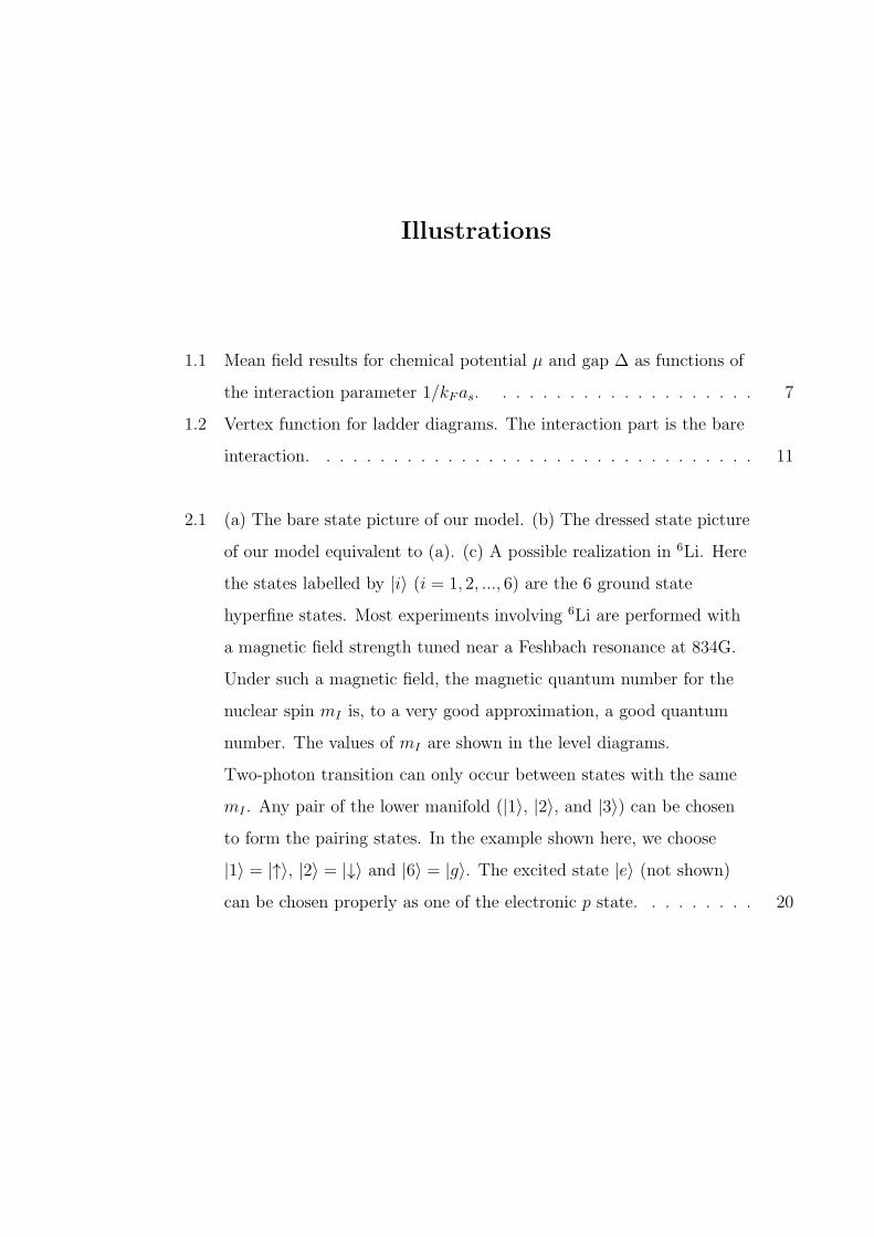
1.1 Mean field results for chemical potential µ and gap ∆ as functions of

the interaction parameter 1/kFas. . . . . . . . . . . . . . . . . . . . 7

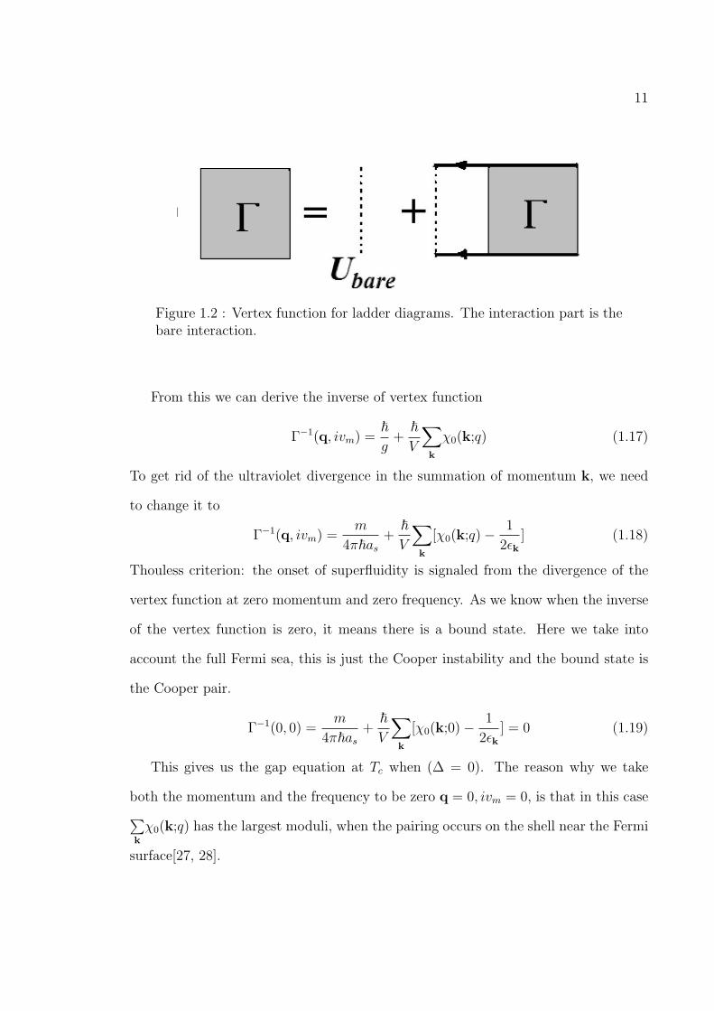
1.2 Vertex function for ladder diagrams. The interaction part is the bare

interaction. . . . . . . . . . . . . . . . . . . . . . . . . . . . . . . . . 11

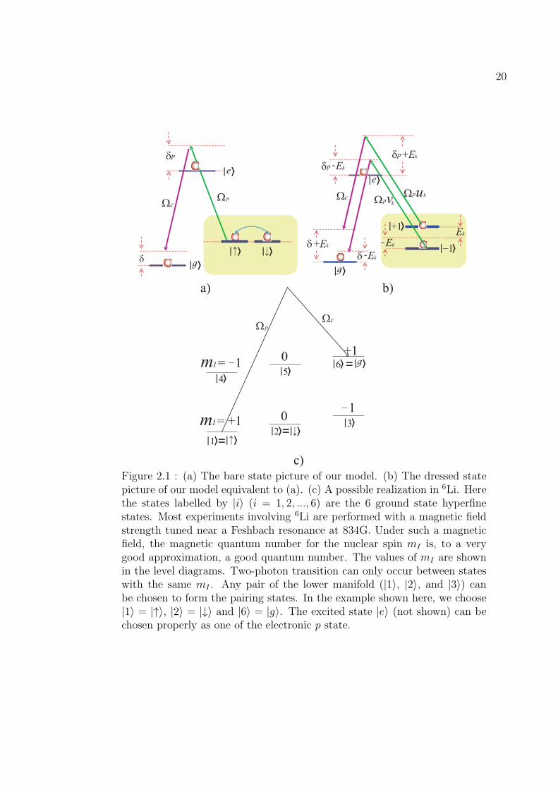
2.1 (a) The bare state picture of our model. (b) The dressed state picture

of our model equivalent to (a). (c) A possible realization in 6Li. Here

the states labelled by |i⟩ (i = 1, 2, ..., 6) are the 6 ground state

hyperfine states. Most experiments involving 6Li are performed with

a magnetic field strength tuned near a Feshbach resonance at 834G.

Under such a magnetic field, the magnetic quantum number for the

nuclear spin mI is, to a very good approximation, a good quantum

number. The values of mI are shown in the level diagrams.

Two-photon transition can only occur between states with the same

mI . Any pair of the lower manifold (|1⟩, |2⟩, and |3⟩) can be chosen

to form the pairing states. In the example shown here, we choose

|1⟩ = |↑⟩, |2⟩ = |↓⟩ and |6⟩ = |g⟩. The excited state |e⟩ (not shown)

can be chosen properly as one of the electronic p state. . . . . . . . . 20

viii

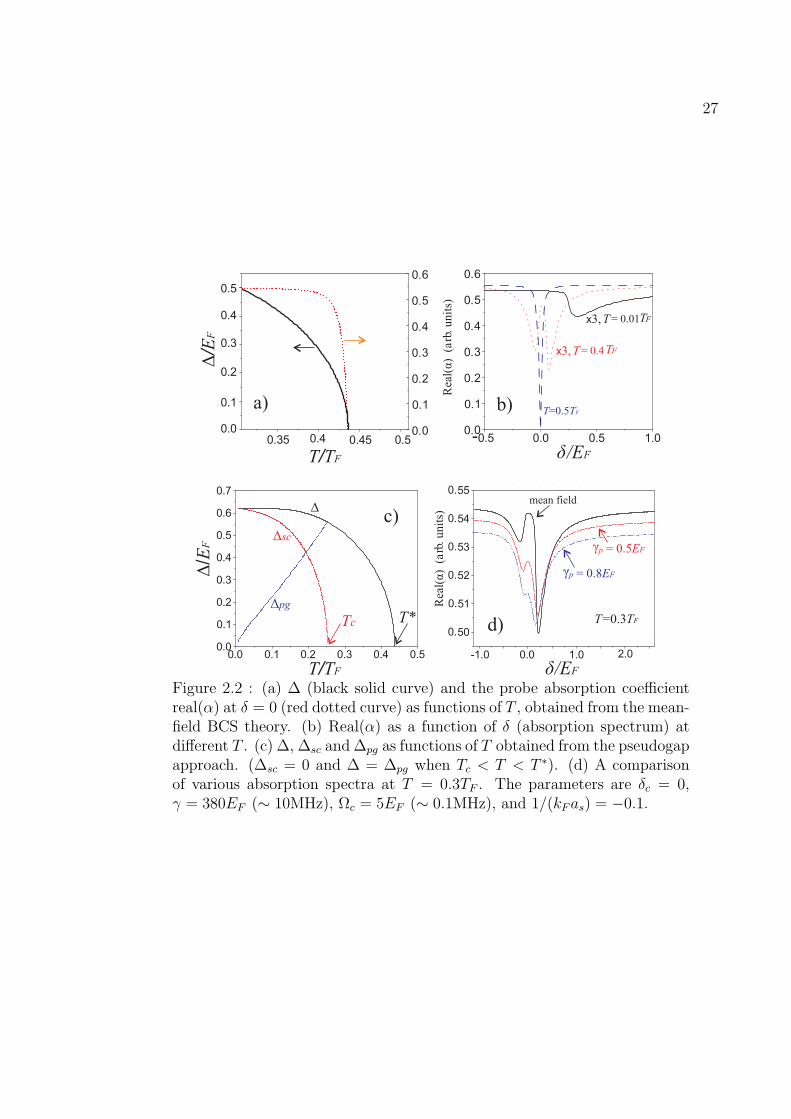
2.2 (a) ∆ (black solid curve) and the probe absorption coefficient real(α)

at δ = 0 (red dotted curve) as functions of T , obtained from the

mean-field BCS theory. (b) Real(α) as a function of δ (absorption

spectrum) at different T . (c) ∆, ∆sc and ∆pg as functions of T

obtained from the pseudogap approach. (∆sc = 0 and ∆ = ∆pg when

Tc < T < T ∗). (d) A comparison of various absorption spectra at

T = 0.3TF . The parameters are δc = 0, γ = 380EF (∼ 10MHz),

Ωc = 5EF (∼ 0.1MHz), and 1/(kFas) = −0.1. . . . . . . . . . . . . . 27

3.1 Left panel: Bound state energies EB as functions of scattering length

for different Zeeman field h. The horizontal dashed lines represent the

threshold energy 2ϵmin. Right panel: Corresponding two-body phase

shifts δ(q = 0, ω) for different Zeeman field h. EB and h are in units

of mλ2/~2, as is in units of ~2/(mλ). . . . . . . . . . . . . . . . . . . 43

3.2 Effective mass γ ≡M⊥/(2m) as functions of scattering length for

different Zeeman field h. h is in units of mλ2/~2, and as is in units of

~2/(mλ). For h ≥ 1, the two-body bound state only exists for as > 0. 45

3.3 Chemical potential µ (a), pairing gap ∆0 (b), and population of

spin-up component n↑ (c) as functions of scattering length as for

different values of the Zeeman field h at λkF/EF = 2. Here

kF = (3π2n)1/3 and EF = ~2k2F/(2m) are the Fermi momentum and

Fermi energy, respectively. . . . . . . . . . . . . . . . . . . . . . . . . 48

3.4 Quasi-particle dispersion spectrum Ek+ (solid lines) and Ek− (dashed

lines) shown in in units of EF for k in the transverse plane (a,

θ = π/2) and along the z-axis (b, θ = 0) for λkF/EF = 2, h/EF = 2. 50

ix

3.5 Pairing fields at unitarity (i.e., 1/as = 0) for h = 0 (top row),

h = 1EF (middle row), h = 2EF (bottom row) and λkF/EF = 2. In

each row, from left to right, we display |⟨ψk↑ψ−k↓⟩|, |⟨ψk↑ψ−k↑⟩| and

|⟨ψk↓ψ−k↓⟩| (all in units of EF ), respectively. . . . . . . . . . . . . . . 51

3.6 Density of states ρ↑ (a) and ρ↓ (b) at unitarity and λkF/EF = 2. . . . 53

3.7 (a) Zero temperature dynamic spin structure factor SS(0, ω) at

unitarity and λkF/EF = 2. (b) Static spin structure factor SS(0) as

functions of the SO coupling strength. . . . . . . . . . . . . . . . . . 57

4.1 Local density of state (arb. units) at the site of a localized

non-magnetic impurity with u = −0.02EFxTF , where EF is the Fermi

energy and xTF =√Naho (aho =

√~/(mω0)) is the Thomas-Fermi

radius of the non-interacting system. The dimensionless interaction

parameter γ = −mg/(~2n0) = 1.25 where n0 = 2√N/(πaho) is the

peak Thomas-Fermi density of the non-interacting system. N = 100

is the total number of particles. The two spin components have equal

population. Solid and dashed lines represent results obtained using

the T -matrix and B-dG method, respectively. The insets show the

density and gap profile of the trapped system from the B-dG

calculation. The units for density, energy and length are n0, EF and

xTF , respectively. . . . . . . . . . . . . . . . . . . . . . . . . . . . . . 76

x

4.2 (a) Density of states for spin up atoms. (b) Density of states for spin

down atoms. (c) Density profiles for both spin species. (d) Gap

profile. In (a) and (b) solid and dashed lines represent results

obtained using the T -matrix and B-dG method, respectively. The

dashed curve in (d) is the gap profile without the impurity. For all

plots, N↑ = N↓ = 50, and u = −0.02EFxTF , where EF is the Fermi

energy and xTF =√Naho is the Thomas-Fermi radius of the

non-interacting system. The harmonic oscillator length and Thomas

Fermi density at the origin are defined by aho =√~/(mω0) and

n0 = 2√N/(πaho). The dimensionless interaction parameter

γ = −mg/(~2n0) = 1.25. The units for density, energy and length are

n0, EF and xTF , respectively. . . . . . . . . . . . . . . . . . . . . . . 78

4.3 Density (left panel) and gap (right panel) profiles of a trapped system

under an extended Gaussian magnetic impurity potential. The width

of the impurity potential is a = 0.2xTF , while the strength is

u = −0.12EFxTF for (a) and (b); u = −0.4EFxTF for (c) and (d),

and u = −1.0EFxTF for (e) and (f). Other parameters and units are

the same as in Fig. 4.2. . . . . . . . . . . . . . . . . . . . . . . . . . . 82

4.4 Density (upper panel, in units of (2EF )3/2/(6π2)) and gap (lower

panel, in units of EF ) profiles along the x-axis of a 3D trapped

system under an extended magnetic impurity potential. The impurity

potential is uniform along the radial direction and has a Gaussian

form with width a = 0.3xTF along the x-axis. The strength of the

impurity is u = −0.07EFxTF . The atom-atom interaction is

characterized by the 3D scattering length as. Here we have used

1/(kFas) = −0.69. . . . . . . . . . . . . . . . . . . . . . . . . . . . . 84

1

Chapter 1

Introduction

In exploring the exotic feature of quantum mechanics, physicists have paid much

attention to bosonic atoms. If one cools Bose gases to the point that their de Broglie

wavelength is comparable to the average distance between atoms, individual atoms

become indistinguishable and their wave functions overlap with each other. Bosonic

atoms fall into the ground state to form Bose Einstein Condensate(BEC). All the

bosonic atoms have the same energy and are said to be degenerate. This could not

happen to fermions as Pauli exclusion principle prohibits two fermions occupying the

same state. Instead, fermions are obliged to fill all the different quantum energy

states, starting from the energy bottom. This is said to constitute a degenerate fermi

gas. BEC has been achieved in 1995 in alkali atoms[1, 2, 3]. To achieve degenerate

fermi gas is more difficult as fermions in the same hyperfine state avoid collisions

which are required for evaporate cooling. To combat this, a JILA group in Boulder

prepared 40K atoms in two different hyperfine states and got the degenerate fermi

gas[4]. When temperature is low, scattering only occurs between atoms of different

hyperfine states.

Fermions can condense if there is attractive interaction between them and they

get paired. The pairing mechanism can be different. In one extreme, atoms are paired

strongly and they can (as molecules) collapse into a Bose-Einstein Condensate. In

the other extreme, atoms can pair weakly and they form correlated state analogous

to Cooper pairs of electrons[5]. In this extreme, we have BCS pairings.

2

BCS theory was developed in 1950’s and is one of the most successful condensed

matter theory[6, 7] ever since. It is originally used to describe superconductivity

for electrons in metal. Electrons form Cooper pairs when there is weak attractive

interaction. A Cooper pair is formed by two electrons with total momentum zero

near the Fermi surface. It can be viewed as a weakly bound boson and it forms

and condenses at the same temperature. BCS theory has also been used to explain

superfluidity in 3He. In solid, the attractive interaction between electrons comes from

the electron-phonon interaction, while in 3He the attractive interaction comes from

the spin fluctuation[8].

In dilute Fermi gases, instead of superconductivity for electron, for charge neutral

atoms, it should be superfluidity. In experiments, atoms are in different hyperfine

states. We use pseudo spins to label these different hyperfine states. The attractive

interaction between two atoms comes directly from atom-atom interaction which is

Van der Waals force. We consider a gas of fermions with the attractive interaction

V . When the interaction is weak, the fermions undergo Cooper instability and form

Cooper pairs. This is a many-body effect as the s-wave scattering length is negative.

There is no two-body bound state. The length of the pair a0 is very large and we

have na30 >> 1, where n is the gas density. Cooper pairs overlap with each other. It

is proper to give them a mean field description.

In cold atoms, although the temperature is cooled below the degenerate temper-

ature, it is very hard to push into the superfluid phase. As we know from BCS

theory, the transition temperature Tc is proportional to exp(−1/|V |) where V is the

interaction strength. For the Van der Waals interaction, Tc is an extremely low tem-

perature. It is hopeless to go to the superfluid phase in ultra-dilute systems where the

interaction strength is very small. This leads to a need for a method to increase the

3

interaction strength and Feshbach resonance is just the method[9, 10]. For Feshbach

resonance, there is a bound state in a closed channel which is energetically unfavor-

able. When the bound state is resonant with the free atoms in the open channel, the

scattering length for atoms in the open channel goes to infinity. Also the energy for

different hyperfine states can be changed using an external magnetic field. Therefore

one can tune the magnetic field to change the strength of the interaction. Using

Feshbach resonance, the superfluid Fermi gas is achieved in 2002[11, 12].

Using Feshabch resonance, we can study the BCS-BEC crossover. The energy

region near a broad resonance, where the s-wave scattering length goes to infinity, is

called the unitary regime. There is only one length scale 1/kF . This is a strongly

correlated system since the interaction between atoms is very strong. The pair size

is comparable to the interparticle spacing. Quantum fluctuation is important in

this region. Fermi gases in the unitary regime represent a type of ”high temperature

superfluid”, as Tc/TF ≈ 0.2 (TF is Fermi temperature), which is much larger than that

for cuprate high temperature superconductors. It is hoped that studies of strongly

interacting Fermi gases may shed light on the long-standing problem of the high Tc

superconductivity.

When the interaction is even stronger, the scattering length is positive. Two

fermions form a bound state and when the temperature is small, they may undergo

Bose-Einstein Condensate. Now the pair length is small, na30 << 1 and the internal

structure of bound pairs is irrelevant. From the BCS regime to the BEC regime, the

physics in different regimes is quite different, however it turns out that it is not a

transition but a crossover. Physical quantities change smoothly from one regime to

another. In this chapter, I will first introduce the mean field theory for T = 0 to see

the crossover, then I will introduce a theory beyond mean field to deal with the T = 0

4

case. In the end, I will show some experiments.

In the next chapter, I will propose one method to detect the fermion pairing

using electromagnetically induced transparency. I will test this method using both

the mean-field model and the pseudogap model. In the third chapter, the ultracold

fermion with the spin-orbit coupling will be presented. I will do the calculation using

the functional integral method. A single classical impurity in Fermi superfluids is

studied in the fourth chapter.

1.1 The Mean Field Theory of the BEC-BCS Crossover

Leggett first gave the general solution for crossover problem at zero temperature[13].

He assumed the system should have a BCS type ground state. The main difference

from the original BCS theory is that for crossover theory, we not only need to consider

the gap profile but also need to conserve the total number. With both gap equation

and number equation taken into account, we have the mean field theory which was

introduced to the ultracold fermion system by many different groups[14, 15, 16].

The temperature is so low that we only need to consider s-wave scattering. For

s-wave scattering, the cross section for fermions within the same hyperfine state is

zero due to the Pauli exclusion principle. We only need to consider the interaction

between hyperfine states. We write the model Hamiltonian as:

H =∑k,σ

ξkc+kσckσ +

∑k,k′,q

Vkk′(q)c+k+q/2,↑c+−k+q/2,↓c−k′+q/2,↓ck′+q/2,↑ (1.1)

where ξk = ϵk − µ = ~2k2/2m− µ is the fermion energy measured from the chemical

potential µ. m is the mass of the atom. Here we only consider the population

balanced and mass balanced case. Vkk′(q) describes the attractive interaction and

as the temperature and density are both extremely low, the detailed structure of the

5

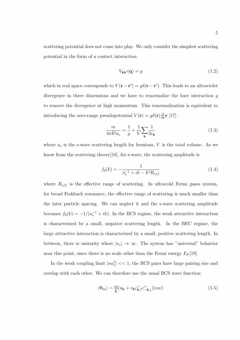
scattering potential does not come into play. We only consider the simplest scattering

potential in the form of a contact interaction.

Vkk′(q) = g (1.2)

which in real space corresponds to V (r− r′) = gδ(r− r′). This leads to an ultraviolet

divergence in three dimensions and we have to renormalize the bare interaction g

to remove the divergence at high momentum. This renormalization is equivalent to

introducing the zero-range pseudopotential V (r) = gδ(r) ∂∂rr [17].

m

4π~2as=

1

g+

1

V

∑k

1

2ϵk(1.3)

where as is the s-wave scattering length for fermions, V is the total volume. As we

know from the scattering theory[18], for s-wave, the scattering amplitude is

f0(k) = − 1

a−1s + ik − k2Reff

(1.4)

where Reff is the effective range of scattering. In ultracold Fermi gases system,

for broad Feshbach resonance, the effective range of scattering is much smaller than

the inter particle spacing. We can neglect it and the s-wave scattering amplitude

becomes f0(k) = −1/(a−1s + ik). In the BCS regime, the weak attractive interaction

is characterized by a small, negative scattering length. In the BEC regime, the

large attractive interaction is characterized by a small, positive scattering length. In

between, there is unitarity where |as| → ∞. The system has ”universal” behavior

near this point, since there is no scale other than the Fermi energy EF [19].

In the weak coupling limit |na3s| << 1, the BCS pairs have large pairing size and

overlap with each other. We can therefore use the usual BCS wave function:

|Φ0s⟩ = Πk(uk + vkc

+k,↑c

+−k,↓)|vac⟩ (1.5)

6

where u2k = 12ξk+Ek

Ek, v2k = −1

2ξk−Ek

Ekand E2

k = ξ2k +∆2.

We can define the superfluid gap parameter,

∆ =∑k

g⟨c+k,↑c+−k,↓⟩ (1.6)

which obeys the self-consistency equation at zero temperature.

∆ =∑k′

g∆

2Ek′(1.7)

which is gap equation at zero temperature. Introducing the function ψk = ∆/Ek, the

gap equation can be written in the form of a Schrodinger equation

(~2k2/m− 2µ)ψk = (1− 2nk)∑k′

gψk′ (1.8)

where nk = v2k = [1− ξkEk

]/2.

When the attractive interaction is strong enough, bound pairs will form with the

energy wq = −ε0+ ~2q2/2M , where ε0 is the binding energy, M = 2m. In the strong

coupling limit, nk ≪ 1, the gap equation reduces to the Schrodinger equation for a

single bound pair.

(~2k2/m− 2µ)ψk =∑k′

gψk′ (1.9)

The chemical potential 2µ plays the role of eigenvalue and 2µ = −ε0 in zeroth order.

In the mean field theory, physical quantities are calculated from the gap equa-

tion together with the number equation. In the weak coupling limit, which is the

BCS limit, µ = EF and ∆ = 8e2e−π/2kF |as|, where EF is Fermi energy and kF

is Fermi momentum. When the interaction strength increases, µ begins to de-

crease and eventually becomes negative in the BEC regime. In the deep BEC side,

µ = − ~22ma2s

+ π~2asnm

= − ε02+ π~2asn

mand ∆ =

√163π

EF√kF as

. The second term is the repul-

sive interaction between molecules. From the mean field theory, the molecule-molecule

7

-2 -1 0 1 2-4

-3

-2

-1

0

1

-2 -1 0 1 20.0

0.5

1.0

1.5

2.0

/EF

1/kFas

/EF

1/kFas

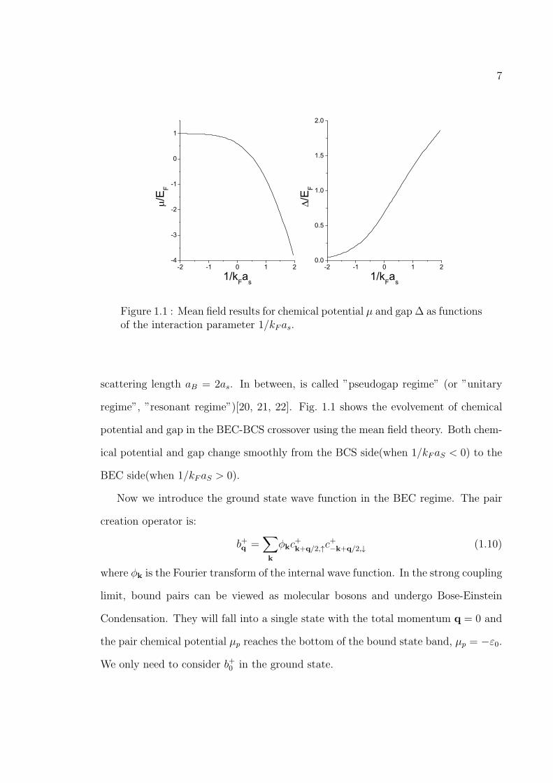
Figure 1.1 : Mean field results for chemical potential µ and gap ∆ as functionsof the interaction parameter 1/kFas.

scattering length aB = 2as. In between, is called ”pseudogap regime” (or ”unitary

regime”, ”resonant regime”)[20, 21, 22]. Fig. 1.1 shows the evolvement of chemical

potential and gap in the BEC-BCS crossover using the mean field theory. Both chem-

ical potential and gap change smoothly from the BCS side(when 1/kFaS < 0) to the

BEC side(when 1/kFaS > 0).

Now we introduce the ground state wave function in the BEC regime. The pair

creation operator is:

b+q =∑k

ϕkc+k+q/2,↑c

+−k+q/2,↓ (1.10)

where ϕk is the Fourier transform of the internal wave function. In the strong coupling

limit, bound pairs can be viewed as molecular bosons and undergo Bose-Einstein

Condensation. They will fall into a single state with the total momentum q = 0 and

the pair chemical potential µp reaches the bottom of the bound state band, µp = −ε0.

We only need to consider b+0 in the ground state.

8

[b0, b+0 ] =

∑k

|ϕk|2(1− 2nk) (1.11)

we can see b+0 represents boson in the strong coupling limit, when nk ≪ 1,∑k

|ϕk|2 = 1,

[b0, b+0 ] = 1.

The ground state is represented by

|Φ0⟩ = [exp(N1/2p b+0 )]|vac⟩ (1.12)

where Np = N/2 is the total number of pairs.

BCS superfluidity may be viewed as Bose-Einstein condensation of weakly bound

Cooper pairs. The strong coupling limit expression Eq.(1.12) can be written in the

BCS form Eq.(1.5) with

vk =N

1/2p ϕk

(1 +Np|ϕk|2)1/2(1.13)

In this way, the ground state wave function goes smoothly from one limit to another

and Eq.(1.5) provides a unified description of the many-body state over the whole

regime.

This mean-field method for zero temperature gives us the basic idea for the

crossover physics and is qualitatively correct compared with experiment. This simple

method is consistent with Bogoliubov-de Gennes theory at zero temperature and sets

a starting point for many theories in population imbalanced system. Also this method

connects to Gross-Pitaevskii theory in the BEC regime.

One disadvantage of the mean field theory is that it omits fluctuations at zero

temperature. The mean field theory drops Hartree shift in the BCS regime[23]; using

the mean field theory, the scattering length between molecular bosons is aB = 2as

in the BEC regime which does not agree with the exact result from the four-body

problem[24] and quantumMonte Carlo calculation[25], where aB ≈ 0.6as. The ground

9

state energy density at the unitarity is of the form Eg/N = (1 + β)(3EF/5), where

(1 + β) = 0.44 from quantum Monte Carlo calculation. In the mean field theory

(1 + β) = 0.59, which is about 34% larger than the quantum Monte Carlo result.

For finite temperature, the mean field calculation gives wrong physical picture

on the BEC side. On the BCS side, transition temperature Tc is defined as the

temperature at which pairs breaking starts to occur and the mean field theory gives

the qualitatively correct answer. But on the BEC side the pairs are deeply bound

and they form molecules and Tc should be defined as the temperature at which the

total momentum q = 0 state has macroscopic occupancy. While the Tc in the mean

field theory on the BEC side is actually the molecular dissociation temperature T ∗.

10

1.2 Ladder Diagrams and Thouless Criterion

Generally speaking, all the methods beyond mean field have to consider pair fluctua-

tion. Using diagram technique, one has to consider ladder diagrams, which describe

the atom scattering accurately in the low density limit. In this section I will present

results from calculating vertex function in ladder diagrams and derive Thouless crite-

rion which provides a criterion for the onset of superfluidity[26]. In the next section

I will introduce the pseudogap method. In chapter 3, the pair fluctuation using

functional integral formalism is calculated.

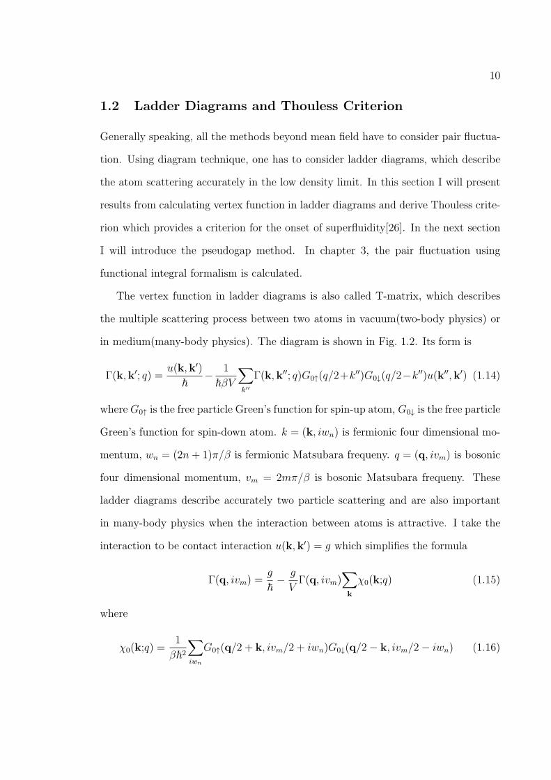
The vertex function in ladder diagrams is also called T-matrix, which describes

the multiple scattering process between two atoms in vacuum(two-body physics) or

in medium(many-body physics). The diagram is shown in Fig. 1.2. Its form is

Γ(k,k′; q) =u(k,k′)

~− 1

~βV∑k′′

Γ(k,k′′; q)G0↑(q/2+k′′)G0↓(q/2−k′′)u(k′′,k′) (1.14)

where G0↑ is the free particle Green’s function for spin-up atom, G0↓ is the free particle

Green’s function for spin-down atom. k = (k, iwn) is fermionic four dimensional mo-

mentum, wn = (2n+ 1)π/β is fermionic Matsubara frequeny. q = (q, ivm) is bosonic

four dimensional momentum, vm = 2mπ/β is bosonic Matsubara frequeny. These

ladder diagrams describe accurately two particle scattering and are also important

in many-body physics when the interaction between atoms is attractive. I take the

interaction to be contact interaction u(k,k′) = g which simplifies the formula

Γ(q, ivm) =g

~− g

VΓ(q, ivm)

∑k

χ0(k;q) (1.15)

where

χ0(k;q) =1

β~2∑iwn

G0↑(q/2 + k, ivm/2 + iwn)G0↓(q/2− k, ivm/2− iwn) (1.16)

11

Figure 1.2 : Vertex function for ladder diagrams. The interaction part is thebare interaction.

From this we can derive the inverse of vertex function

Γ−1(q, ivm) =~g+

~V

∑k

χ0(k;q) (1.17)

To get rid of the ultraviolet divergence in the summation of momentum k, we need

to change it to

Γ−1(q, ivm) =m

4π~as+

~V

∑k

[χ0(k;q)−1

2ϵk] (1.18)

Thouless criterion: the onset of superfluidity is signaled from the divergence of the

vertex function at zero momentum and zero frequency. As we know when the inverse

of the vertex function is zero, it means there is a bound state. Here we take into

account the full Fermi sea, this is just the Cooper instability and the bound state is

the Cooper pair.

Γ−1(0, 0) =m

4π~as+

~V

∑k

[χ0(k;0)−1

2ϵk] = 0 (1.19)

This gives us the gap equation at Tc when (∆ = 0). The reason why we take

both the momentum and the frequency to be zero q = 0, ivm = 0, is that in this case∑k

χ0(k;q) has the largest moduli, when the pairing occurs on the shell near the Fermi

surface[27, 28].

12

1.3 Pseudogap Method

Using the Thouless criterion together with number conservation we can get the tran-

sition temperature for BCS-BEC crossover[29, 30]. In order to get the physics in

superfluid phase, one way is to calculate the scattering process, the vertex function,

in the symmetry-breaking phase[31, 32, 33]. Here I introduce another method which

is called the pseudogap method[34, 35]. It gives a more clear description and although

some approximations are made, it still catches most of the BCS-BEC physics.

Let us define the four dimensional form

χ(q) =1

V

∑k

[χ0(k;q)−1

2ϵk] (1.20)

Γ(q) = Γ(q, ivm) (1.21)

Here we only consider population balanced system.

Γ−1(0) = 0 gives the gap equation. And in the superfluid region when T ≤ Tc,

the vertex function can be divided into two parts.

Γ(q) = Γsc(q) + Γpq(q) (1.22)

where Γsc(q) represents the condensed Cooper pairs part, Γpq(q) represents pseudogap

part which does not condense.

The superfluid vertex function and self energy are given, respectively, by

Γsc(q) = −β∆2scδ(q)

Σsc(q) =1

β~V∑q

Γsc(q)G0(q − k)

= −1

~∆2scG0(−k) (1.23)

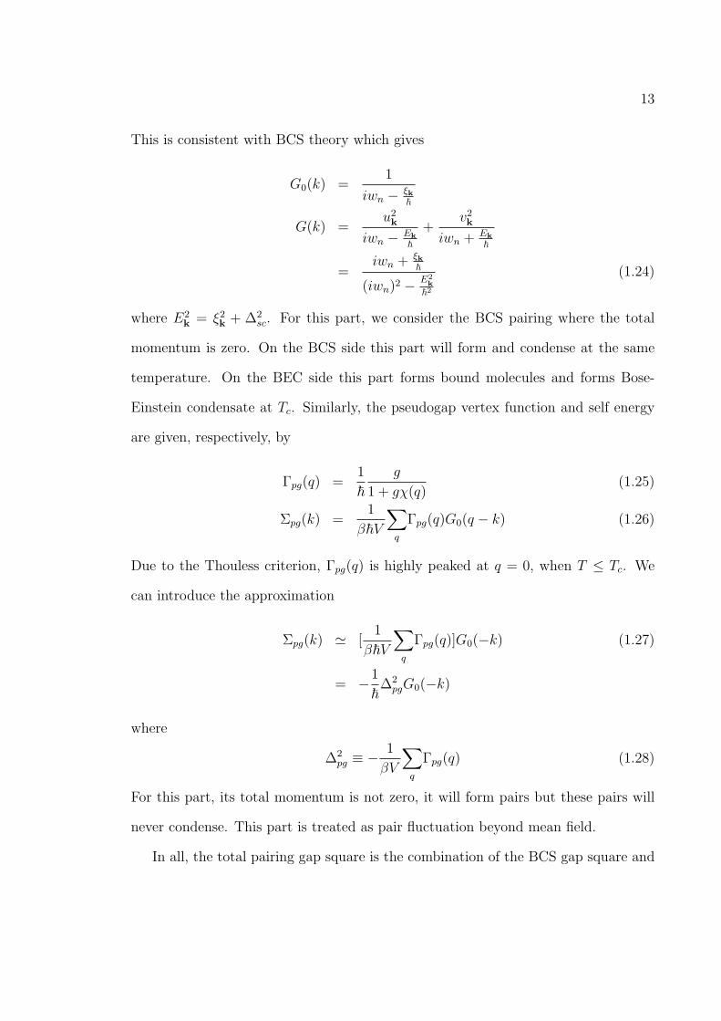
13

This is consistent with BCS theory which gives

G0(k) =1

iwn − ξk~

G(k) =u2k

iwn − Ek

~

+v2k

iwn +Ek

~

=iwn +

ξk~

(iwn)2 −E2

k

~2

(1.24)

where E2k = ξ2k + ∆2

sc. For this part, we consider the BCS pairing where the total

momentum is zero. On the BCS side this part will form and condense at the same

temperature. On the BEC side this part forms bound molecules and forms Bose-

Einstein condensate at Tc. Similarly, the pseudogap vertex function and self energy

are given, respectively, by

Γpg(q) =1

~g

1 + gχ(q)(1.25)

Σpg(k) =1

β~V∑q

Γpg(q)G0(q − k) (1.26)

Due to the Thouless criterion, Γpg(q) is highly peaked at q = 0, when T ≤ Tc. We

can introduce the approximation

Σpg(k) ≃ [1

β~V∑q

Γpg(q)]G0(−k) (1.27)

= −1

~∆2pgG0(−k)

where

∆2pg ≡ − 1

βV

∑q

Γpg(q) (1.28)

For this part, its total momentum is not zero, it will form pairs but these pairs will

never condense. This part is treated as pair fluctuation beyond mean field.

In all, the total pairing gap square is the combination of the BCS gap square and

14

the pseudogap square. we have

∆2 = ∆2sc +∆2

pg

E2k = ξ2k +∆2

u2k =1

2

ξk + Ek

Ek

v2k = −1

2

ξk − Ek

Ek

(1.29)

Finally we get

GAP equation

Γ−1(0) = 0 (1.30)

NUMBER equation

N =2

β~V∑k

G(k) (1.31)

We use these two equations to get the total gap where the transition temperature

relates to T ∗.

PSEUDOGAP equation

∆2pg = − 1

βV

∑q

Γpg(q) (1.32)

We use this equation to calculate the pseudogap. The real transition temperature

Tc appears when

∆2 = ∆2pg (1.33)

This method catches the main physics in the BCS-BEC crossover and gives a

qualitative picture both at zero temperature and above zero temperature.

15

1.4 Radio Frequency Experiment

The experimental signatures of fermionic pairing and superfluidity in ultracold gases

of 40K and 6Li include measurements of the condensate momentum, density distribution[37,

38, 36], the pairing gap[39], and the observation of vortex lattices in rotating clouds[40].

Here we mainly introduce the observation of the pairing gap in a strongly interact-

ing fermi gas using radio frequency spectroscopy(RF). This was first carried out in

Rudolf Grimm’s group in Innsbruck. They prepared their ultracold gas of fermionic

6Li atoms in a balanced spin mixture of two lowest hyperfine states |1⟩ and |2⟩. A

magnetic field B is applied for the Feshbach detuning through a broad resonance

centered at B0 = 830G. The superfluid state originates from pairings of atoms in

states |1⟩ and |2⟩. Radio frequency(RF) fields are used for transferring atoms out of

the superfluid state to a normal state. The field drives a transition from state |2⟩ to

an empty state |3⟩ which is another hyperfine state and is not paired. This idea is

closely related to observing the superconductor-normal metal current for electrons. It

reflects the density of states and displays the excitation gap. The RF field detuning

is δ = ERF − (E3 − E2), where ERF , E3, and E2 are the energies of the RF photon

and of the states |3⟩ and |2⟩, respectively.

The radio frequency signal is shown by fractional loss in state |2⟩ for various

magnetic fields and temperatures. A signal of the pairing process is the emergence of

a double-peak structure in the spectral response as a result for both the unpaired and

paired atoms. When the temperature is high, there is no pairing, all the atoms in state

|2⟩ are unpaired and in normal state. This corresponds to a relatively narrow atomic

peak at the original position in the spectra. When the temperature becomes lower,

there appears another board peak which is located at a higher frequency. This is

because energy is required for pair breaking. When temperature becomes even lower,

16

the unpaired narrow peak disappears. Now all the atoms in state |2⟩ are paired.

In theory, transitions using the RF field is introduced as a perturbation and one

can use the standard linear-response theory. A theoretic calculation using the method

for two channel model and also adding the local density approximation can produce

a similar picture[41]. On the BEC side, the energy difference between two peaks fails

to be exactly the molecular binding energy but just relates to it, while on the BCS

side it relates to the pairing gap.

This is called the first generation radio frequency experiment in ultracold fermions.

The signal is averaged over the whole trap. The double peak structure may come from

the trap inhomogeneity[42]. In the trap center, it is in superfluid phase while at the

trap edge, due to small density, it is still in normal state. The first generation radio

frequency experiment records both the signals from the trap center and edge.

Another phenomenon that will complicate the radio frequency spectrum is the

final state effect. In above we have assumed state |3⟩ is only connected to the system

from radio frequency. As for 6Li at magnetic field near B0 = 830G, it is not the

case. |3⟩ has the big s-wave scattering length with state |1⟩ and |2⟩. So in modeling,

we have to consider interactions between all three states, which makes the system

complicated to handle[43, 44, 45, 46, 47, 48]. Fortunately, we can lessen the final

state effect in some cases. For 40K case, the final state effect is very small. For 6Li,

we can rearrange the experimental set up. For example, first make the superfluid

state using state |1⟩ and |3⟩ and then use radio frequency to transport atoms from

|3⟩ to |2⟩[49, 50]. In this way, the final state effect is small.

Complicated by the trap inhomogeneity and the final state effect, the first gen-

eration RF experiment is hard to interpret quantitatively. Then comes the second

generation experiment. The JILA group use time-of-flight imaging to detect mo-

17

mentum distribution for state |3⟩. In this way they get momentum resolved radio

frequency spectroscopy[51, 52]. By varying momentum and detuning energy, they

can get the graph for spectral function A(k, w). Recently there is also proposal from

their group that they can detect the signal only from trap center. In this way, they

can get spectral function for a localized region, hence overcome the inhomogeneity

problem.

Spatially resolved RF spectroscopy has been realized by the MIT group[53]. In

their experiment, they use phase-contrast imaging to detect density differences be-

tween two hyperfine states. For example, if the RF field is shining along the y axis,

they can get the two-dimensional density difference in the xz plane which has inte-

grated density difference along the y axis. If there is cylindrical symmetry in the

system along the z axis, one two-dimensional picture gives all the information. The

three dimensional radial profile is calculated using the inverse Abel transformation

from the two-dimensional profile. If there is not cylindrical symmetry along z axis.

More two-dimensional information is needed along different directions in the xy plane.

In this way, they can have the local radio frequency spectrum at each site. The spatial

resolution is 1.4 um which is of the order of Fermi wavelength.

In chapter 2, we propose another measurement for the superfluid pairing. Fur-

thermore, in chapter 4, we propose a modified RF experiment designed to allow direct

determination of the local density of states.

18

Chapter 2

Detection of Fermi Pairing via Electromagnetically

Induced Transparency

2.1 Introduction

A unique phenomenon of low temperature Fermi systems is the formation of correlated

Fermi pairs when there is attractive interaction. How to detect pair formation in

an indisputable fashion has remained a central problem in the study of ultracold

atomic physics. Unlike the BEC transition of bosons for which the phase transition

is accompanied by an easily detectable drastic change in atomic density profile, the

onset of pairing in Fermi gases does not result in dramatic change that is measurable

in fermion density. Early proposals sought the BCS pairing signature from the images

of off-resonance scattered light [54, 55]. The underlying idea is that, in order to gain

pairing information, measurement must go beyond the first-order coherence and, for

example, use the density-density correlation. This is also the foundation for other

detection methods such as spatial noise correlations in the image of the expanding gas

[56], Bragg scattering [57, 58, 59, 60, 61, 62, 63], Raman spectroscopy [64, 65], Stokes

scattering method [66], radio frequency (RF) spectroscopy [39, 41], optical detection

of absorption [67], and interferometric method [68]. Among all these methods, RF

spectroscopy [39, 41] has been the one of greatest use in current experiments [69, 70].

In this chapter, we propose an alternative detection scheme, whose principle of

operation is illustrated in Fig. 2.1(a). In our scheme, we use two laser fields, a rela-

19

tively strong coupling and a weak probe laser field between the excited state |e⟩ and,

respectively, the ground state |g⟩ and the spin up state |↑⟩, forming a Λ-type energy

diagram, which facilitates the use of electromagnetically induced transparency (EIT)

to determine the nature of pairing in the interacting Fermi gas of two hyperfine spin

states: |↑⟩ and |↓⟩. EIT [71, 72] is defined as a probe laser field experiencing virtu-

ally no absorption but steep dispersion when operating around an atomic transition

frequency. It has been at the forefront of many exciting developments in the field of

quantum optics [73]. Such a phenomenon is based on quantum interference, which is

absent in measurement schemes such as in Ref. [66], where lasers are tuned far away

from single-photon resonance. In the context of ultracold atoms, an important ex-

ample of EIT is the experimental demonstration of dramatic reduction of light speed

in the EIT medium in the form of Bose condensate [74, 75]. This experiment has led

to a renewed interest in EIT, motivated primarily by the prospect of the new possi-

bilities that the slow speed and low intensity light may add to nonlinear optics [76]

and quantum information processing [77, 78]. More recently, EIT has been used to

spectroscopically probe ultracold Rydberg atoms [79]. In this chapter, we will show

how EIT can be used to detect the nature of pairing in Fermi gases.

Before we go into detail, let us first compare the proposed EIT method with the

RF spectroscopy method which is widely used nowadays in probing Fermi gases. In

the RF experiment, an atomic sample is prepared and an RF pulse is applied to

the sample which couples one of the pairing states, say state | ↑⟩, to a third atomic

level |3⟩. This is followed by a destructive measurement of the transferred atom

numbers using absorption laser imaging. The RF signal is defined as the average

rate change of the population in state |3⟩ during the RF pulse, which can be inferred

from the measured loss of atoms in | ↑⟩. This process is repeated for another RF

20

|d

dp

Wc

|

Wp

dp -Ek

Wpuk

Wpvk

dp +Ek

d +Ek

↑ ↓› ›

|g›|g›

|e›|e›

|+1›

|−1›−

a) b)

|↓›|2›|1›

|5›

|3›

|4›

|6›

|↑›=

=

|g›=

WcWp

mI = +1

mI = 1−0

0

+1

1−

c)

Wc

d -Ek

Ek

Ek

Figure 2.1 : (a) The bare state picture of our model. (b) The dressed statepicture of our model equivalent to (a). (c) A possible realization in 6Li. Herethe states labelled by |i⟩ (i = 1, 2, ..., 6) are the 6 ground state hyperfinestates. Most experiments involving 6Li are performed with a magnetic fieldstrength tuned near a Feshbach resonance at 834G. Under such a magneticfield, the magnetic quantum number for the nuclear spin mI is, to a verygood approximation, a good quantum number. The values of mI are shownin the level diagrams. Two-photon transition can only occur between stateswith the same mI . Any pair of the lower manifold (|1⟩, |2⟩, and |3⟩) canbe chosen to form the pairing states. In the example shown here, we choose|1⟩ = |↑⟩, |2⟩ = |↓⟩ and |6⟩ = |g⟩. The excited state |e⟩ (not shown) can bechosen properly as one of the electronic p state.

21

pulse with a different frequency. In addition to sparking many theoretical activities

[43, 44, 45, 46, 47, 48], this method has recently been expanded into the imbalanced

Fermi gas systems, where pairing can result in a number of interesting phenomena

[80, 81]. A disadvantage of this method is its inefficiency: The sample must be

prepared repeatedly for each RF pulse. In addition, as we mentioned in the first

chapter, for the most commonly used fermionic atom species, i.e., 6Li, the state |3⟩

interacts strongly with the pairing states due to the fact that all three states involved

have pairwise Feshbach resonances at relatively close magnetic field strengths. This

leads to the so-called final state effect which greatly complicates the interpretation of

the RF spectrum.

In the EIT method, by contrast, one can directly measure the absorption or trans-

mission spectrum of the probe light. If we apply a frequency scan faster than the

lifetime of the atomic sample to the weak probe field, the whole spectrum can be

recorded continuously in a nearly non-destructive fashion to the atomic sample. Fur-

thermore, the EIT signal results from quantum interference and is extremely sensitive

to the two-photon resonance condition. The width of the EIT transparency window

can be controlled by the coupling laser intensity and be made narrower than EF .

As we will show below, this property can be exploited to detect the onset of pairing

as the pairing interaction shifts and destroys the two-photon resonance condition.

In addition, due to different selection rules compared with the RF method, one can

pick a different final state whose interaction with the pairing states are negligible [see

Fig. 2.1(c)], hence avoiding the final state effects.

The chapter is organized as follows. In Sec. 2.2, we described the model under

study and define the key quantity of the proposal — the absorption coefficient of

the probe light. In Sec. 2.3, we present the expression of the probe absorption coef-

22

ficient and construct a quasiparticle picture that will become convenient to explain

the features of the spectrum. In Sec. 2.4, we include the derivation of the pairing

fluctuations in the framework of the pseudogap theory [35]. The results are presented

in Sec. 2.5, where spectral features at different temperatures are explained. We also

show how the EIT spectrum can be used to detect the onset of pairing.

2.2 Model

Let us now describe our model in more detail, beginning with the definition of ωi and

Ωi as the temporal and Rabi frequencies of the probe (i = p) and coupling (i = c)

laser field. The two laser fields have an almost identical wavevector kL (along z

direction). The system to be considered is a homogeneous one with a total volume

V , and can thus be described by operators ak,i (a†k,i) for annihilating (creating) a

fermion in state |i⟩ with momentum ~k, and kinetic energy ϵk = ~2k2/2m, where

m is the atomic mass. Here, ak,i are defined in an interaction picture in which

ak,e = a′k,ee−iωpt, ak,g = a′k,ge

i(ωc−ωp)t, and ak,σ = a′k,σ (σ =↑, ↓), where a′k,i are the

corresponding Schrodinger picture operators.

In a probe spectrum, the signal to be measured is the probe laser field, which

is modified by a polarization having the same mathematical form as the probe field

according to [82]

∂Ωp

∂z+

1

c

∂Ωp

∂t= i

µ0ωpcde↑2

Pp ≡ αΩp , (2.1)

where Pp is the slowly varying amplitude of that polarization, dij is the matrix element

of the dipole moment operator between states |i⟩ and |j⟩, and µ0 and c are the

magnetic permeability and the speed of light in vacuum, respectively. The parameter

α in Eq. (2.1) represents the complex absorption coefficient of the probe light [82].

By performing an ensemble average of the atomic dipole moment, we can express α

23

as

α = iα0

Ωp

1

V

∑k,q

⟨a†q,↑ak+kL,e

⟩ei(k−q)·r, (2.2)

where α0 ≡ µ0ωpc |de↑|2. The real and imaginary part of α correspond to the probe

absorption spectrum and dispersion spectrum, respectively.

To determine the probe spectrum, we start from the grand canonical Hamiltonian

H =∑

k

(H1k + H2k + H3k

), where

H1k = (ξk − δp) a†k,eak,e + (ξk − δ) a†k,gak,g ,

H2k = −1

2(Ωca

†k+kL,e

ak,g + Ωpa†k+kL,e

ak,↑)− h.c ,

H3k =∑σ

ξka†k,σak,σ − (∆a†k,↑a

†−k,↓ + h.c) , (2.3)

describe the bare atomic energies of states |e⟩ and |g⟩, the dipole interaction between

atoms and laser fields, and the mean-field Hamiltonian for the spin up and down

subsystem, respectively. Here, ξk = ϵk − µ with µ being the chemical potential, δp =

~ (ωp − ωe↑) and δc = ~ (ωc − ωeg) are the single-photon detunings, and δ = δp − δc is

the two-photon detuning with ωij being the atomic transition frequency from level |i⟩

to |j⟩. In arriving at H3k, in order for the main physics to be most easily identified,

we have expressed the collisions between atoms of opposite spins in terms of the gap

parameter ∆ = −UV −1∑

k⟨a−k,↓ak,↑⟩ under the assumption of BCS paring, where U

characterizes the contact interaction between | ↑⟩ and | ↓⟩ which, in the calculation,

will be replaced in favor of the s-wave scattering length as via the regularization

procedure:

m

4π~2as=

1

U+

1

V

∑k

1

2ϵk. (2.4)

A more complex model including the pseudo-gap physics [35] will be presented later

in the chapter. Finally, we note that the effect of the collisions involving the final

24

state |g⟩ in the RF spectrum has been a topic of much recent discussion. In our

model, the spectra are not limited to the RF regime, and this may provide us with

more freedom to choose |g⟩ (and |e⟩) that minimizes the final state effect. In what

follows, for the sake of simplicity, we ignore the collisions involving states |g⟩ (and

|e⟩). In practice, the effects of final state interaction can be minimized by choosing

the proper atomic species [51] or hyperfine spin states [50]. In the example shown in

Fig. 2.1(c), it is indeed expected that |g⟩ does not interact strongly with either of the

pairing state.

2.3 Quasiparticle Picture

The part of the Hamiltonian describing the pairing of the fermions can be diagonalized

using the standard Bogoliubov transformation:

ak,↑ = ukαk,↑ + vkα†−k,↓ ,

a†−k,↓ = −vkαk,↑ + ukα†−k,↓ , (2.5)

where uk =√(Ek + ξk) /2Ek, vk =

√(Ek − ξk) /2Ek, and Ek =

√ξ2k +∆2 is the

quasiparticle energy dispersion. Now we introduce two sets of quasiparticle states

| ± 1k⟩, representing the electron and hole branches, respectively. The corresponding

field operators are defined as

αk,+1 ≡ αk,↑ , αk,−1 ≡ α†−k,↓ , (2.6)

in terms of which, the grand canonical Hamiltonian can be written as

25

H =∑k

[(ξk − δp) a

†k,eak,e + (ξk − δ) a†k,gak,g + Ekα

†k,+1αk,+1 − Ekα

†k,−1αk,−1

−(Ωc

2a†k+kL,e

ak,g + h.c.

)−(Ωpuk2

a†k+kL,eαk,+1 + h.c

)−(Ωpvk2

a†k+kL,eαk,−1 + h.c

)].

(2.7)

A physical picture emerges from this Hamiltonian very nicely. The state |+1k⟩ (|−1k⟩)

has an energy dispersion +Ek (−Ek) and is coupled to the excited state |e⟩ by an

effective Rabi frequency Ωpuk (Ωpvk), which is now a function of k. In the quasiparticle

picture, our model becomes a double Λ system as illustrated in Fig. 2.1(b). Let +Λ

(−Λ) denote the Λ configuration involving |+1k⟩ (|−1k⟩). The +Λ (−Λ) system is

characterized with a single-photon detuning of δp + Ek (δp − Ek) and a two-photon

detuning of δ+Ek (δ−Ek). In thermal equilibrium at temperature T (in the absence

of the probe field), we have

⟨α†k,+1αk′,+1⟩ = δk,k′ − ⟨α†

k,−1αk′,−1⟩ = δk,k′f (Ek) , (2.8)

where

f (ω) = [exp (ω/kBT ) + 1]−1 , (2.9)

is the standard Fermi-Dirac distribution for quasiparticles. Thus, as temperature

increases from zero, the probability of finding a quasiparticle in state |+1k⟩ increases

while that in state |−1k⟩ decreases but the total probability within each momentum

group remains unchanged. Similarly, in the quasiparticle picture, the probe spectrum

receives contributions from two transitions

α = iα0

Ωp

1

V

∑k,q

ei(k−q)·r×

[uqρe,+1 (k+ kL,q) + vqρe,−1 (k+ kL,q)] , (2.10)

26

where ρi,±1 (k,k′) =

⟨α†k′,±1ak,i

⟩are the off-diagonal density matrix elements in mo-

mentum space.

The equations for the density matrix elements can be obtained by averaging, with

respect to the thermal equilibrium defined in Eq. (2.8), the corresponding Heisenberg’s

equations of motion based upon Hamiltonian (2.3). In the regime where the linear

response theory holds, the terms at the second order and higher can be ignored, and

the density matrix elements correct up to the first order in Ωp are then found to be

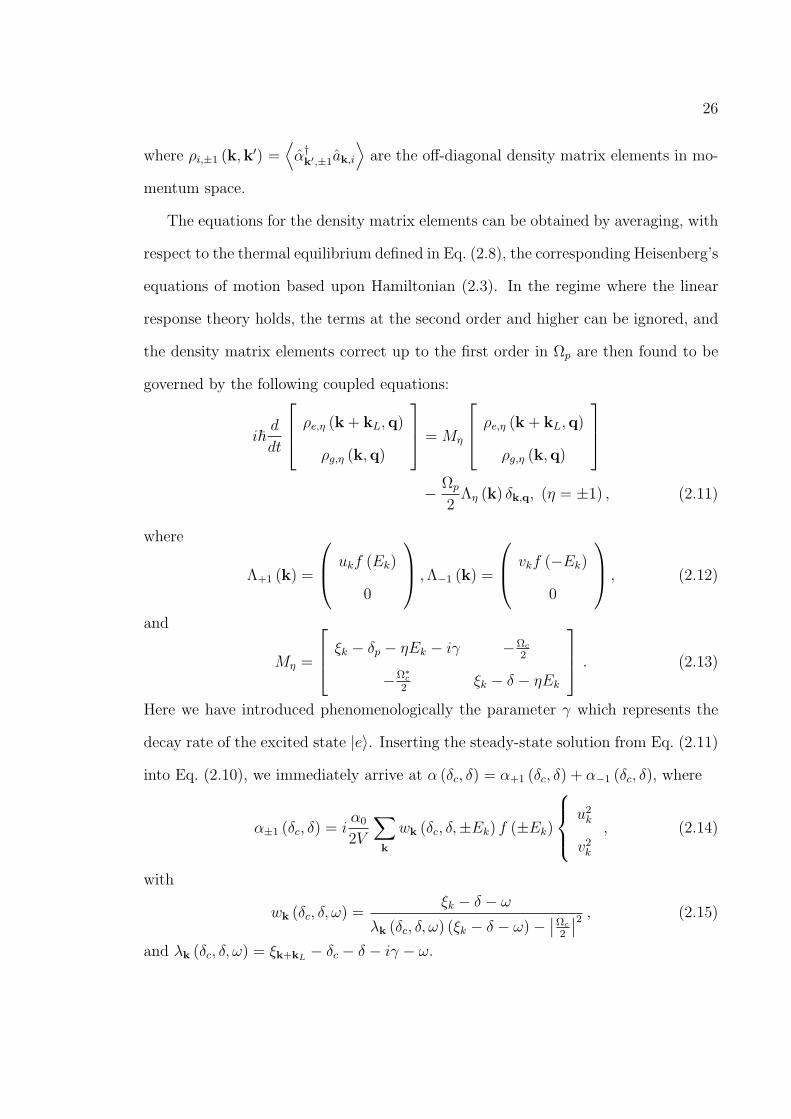
governed by the following coupled equations:

i~d

dt

ρe,η (k+ kL,q)

ρg,η (k,q)

=Mη

ρe,η (k+ kL,q)

ρg,η (k,q)

− Ωp

2Λη (k) δk,q, (η = ±1) , (2.11)

where

Λ+1 (k) =

ukf (Ek)

0

,Λ−1 (k) =

vkf (−Ek)

0

, (2.12)

and

Mη =

ξk − δp − ηEk − iγ −Ωc

2

−Ω∗c

2ξk − δ − ηEk

. (2.13)

Here we have introduced phenomenologically the parameter γ which represents the

decay rate of the excited state |e⟩. Inserting the steady-state solution from Eq. (2.11)

into Eq. (2.10), we immediately arrive at α (δc, δ) = α+1 (δc, δ) + α−1 (δc, δ), where

α±1 (δc, δ) = iα0

2V

∑k

wk (δc, δ,±Ek) f (±Ek)

u2k

v2k

, (2.14)

with

wk (δc, δ, ω) =ξk − δ − ω

λk (δc, δ, ω) (ξk − δ − ω)−∣∣Ωc

2

∣∣2 , (2.15)

and λk (δc, δ, ω) = ξk+kL− δc − δ − iγ − ω.

27

Figure 2.2 : (a) ∆ (black solid curve) and the probe absorption coefficientreal(α) at δ = 0 (red dotted curve) as functions of T , obtained from the mean-field BCS theory. (b) Real(α) as a function of δ (absorption spectrum) atdifferent T . (c) ∆, ∆sc and ∆pg as functions of T obtained from the pseudogapapproach. (∆sc = 0 and ∆ = ∆pg when Tc < T < T ∗). (d) A comparisonof various absorption spectra at T = 0.3TF . The parameters are δc = 0,γ = 380EF (∼ 10MHz), Ωc = 5EF (∼ 0.1MHz), and 1/(kFas) = −0.1.

28

2.4 Pseudogap Picture

In this section, we generalize the result of Eq. (2.2) for α from the mean-field BCS

pairing to a more realistic situation where pair fluctuations are included in the form

of a pseudogap. The process uses the linear response theory [83] which is familiar in

the field of condensed matter physics.

First, let us highlight the results of pseudogap theory [35] that are relevant to

our EIT spectrum calculation. When pairing fluctuations at finite temperature are

included in the framework of the pseudogap model [35], the BCS gap equation and

number equation are still valid. However, the gap ∆ is now regarded as the total gap

divided into a BCS gap ∆sc for condensed (BCS) pairs below Tc and a pseudogap ∆pg

for preformed (finite momentum) pairs:

∆2 = ∆2sc +∆2

pg . (2.16)

The onset of the total gap ∆ occurs at temperature T ∗, which is greater than Tc. The

system with preformed pairs is described by the Green’s function

G−1(k, iwn) = G−10 (k, iwn)− Σ(k, iwn), (2.17)

where the non-interacting Green’s function

G0(k, iwn) = (iωn − ξk)−1 , (2.18)

and the self energy

Σ(k, iwn) = Σsc(k, iwn) + Σpg(k, iwn)

=∆2sc

iwn + ξk+

∆2pg

iwn + ξk + iγp, (2.19)

with wn being the Fermi Matsubara frequency and γ−1p the finite lifetime of pseudogap

pairs. The spectral function A(k, ω) can be obtained from the Green’s function via

29

the relation

A(k, ω) = −2 ImG(k, ω + i0+

), (2.20)

which, with the help of Eqs. (2.17), (2.18), and (2.19), is found to be given by

A(k, ω) =2(ω + ξk)

2γp∆2pg

[ω2 − E2k ]

2(ω + ξk)2 + γ2p [ω2 − Esc2

k ]2, (2.21)

where Esck =

√ξk

2 +∆2sc. In the limit of γp → 0 and Esc

k → Ek, we recover from Eq.

(2.21) the spectral function under the BCS paring

A(k, w) = 2π[u2kδ(ω − Ek) + v2kδ(ω + Ek)] . (2.22)

In order to use the linear response theory, we first divide our system into a “left

part” comprising two hyperfine spin states: |↑⟩ and |↓⟩, a “right part” consisting of

the coupling laser field and states |g⟩ and |e⟩, described by the Hamiltonian

HR =∑k

[(ξ−k δp)a

†k,eak,e + (ξk − δ)a†k,gak,g

]−

(Ωc

2

∑k

a†k+kL,eak,g + h.c.

), (2.23)

and finally the coupling between the two parts induced by the probe field, described

by the tunneling Hamiltonian

HT = −Ωp

2

∑k

a†k+kL,eak,↑ + h.c

≡ A+ A†. (2.24)

Next, we change HR into a diagonal form

HR =∑k

[Eαk α

†kαk + Eβ

k β†kβk

], (2.25)

in terms of a pair of dressed state operators, α and β, defined via the transformation ak+kL,e

ak,g

=

uαk uβk

vαk vβk

αk

βk

, (2.26)

30

where

(uα,βk )2 = (vβ,αk )2 =1

2

(1± ζk − ηk√

(ζk − ηk)2 + |Ωc|2

), (2.27)

Eα,βk =

1

2

(ζk + ηk ±

√(ζk − ηk)2 + |Ωc|2

), (2.28)

with ζk = ξk+kL − δp and ηk = ξk − δ. In terms of the dressed state operators, A

becomes

A = −Ωp

2

∑k

[uαk α

†kak,↑ + uβk β

†kak,↑

](2.29)

and is in a form to which the linear response theory [83] is directly applicable. Fol-

lowing the standard practice, we then find

⟨A⟩ =Ω2p

4

∑k

∑η=α,β

(uηk)2

+∞∫−∞

dωL2π

AL(k, ωL)

+∞∫−∞

dωR2π

AηR(k, ωR)f(ωR)− f(ωL)

ωR − ωL + i0+. (2.30)

In Eq. (2.30), AL(k, ωL) is same as A(k, ωL) defined in Eq. (2.21), while AηR(k, ωR)

is given by 2πδ (ωR − Eηk) because the right part is in a normal state described by

the Green’s function G−1η (k, iwn) = iwn − Eη

k . Integrating over ωR, we change Eq.

(2.30) into

⟨A⟩ =Ω2p

4

∑k

∑η=α,β

(uηk)2

+∞∫−∞

dω

2πA(k, ω)

f(Eηk)− f(ω)

Eηk − ω + i0+

, (2.31)

where the dummy variable ωL has been changed into ω. We now include the effect of

the decay of the excited state phenomenologically by replacing δp with δp − iγ. We

see that Eηk now becomes imaginary which signals the inability of the dressed states

to hold populations. This along with the fact that the dressed states here are the

superpositions of the initially empty states provide us with the justification to set

31

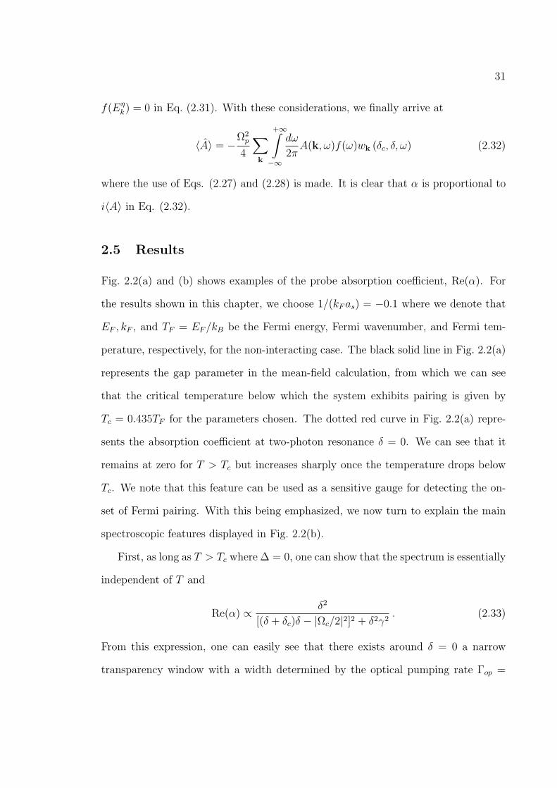
f(Eηk) = 0 in Eq. (2.31). With these considerations, we finally arrive at

⟨A⟩ = −Ω2p

4

∑k

+∞∫−∞

dω

2πA(k, ω)f(ω)wk (δc, δ, ω) (2.32)

where the use of Eqs. (2.27) and (2.28) is made. It is clear that α is proportional to

i⟨A⟩ in Eq. (2.32).

2.5 Results

Fig. 2.2(a) and (b) shows examples of the probe absorption coefficient, Re(α). For

the results shown in this chapter, we choose 1/(kFas) = −0.1 where we denote that

EF , kF , and TF = EF/kB be the Fermi energy, Fermi wavenumber, and Fermi tem-

perature, respectively, for the non-interacting case. The black solid line in Fig. 2.2(a)

represents the gap parameter in the mean-field calculation, from which we can see

that the critical temperature below which the system exhibits pairing is given by

Tc = 0.435TF for the parameters chosen. The dotted red curve in Fig. 2.2(a) repre-

sents the absorption coefficient at two-photon resonance δ = 0. We can see that it

remains at zero for T > Tc but increases sharply once the temperature drops below

Tc. We note that this feature can be used as a sensitive gauge for detecting the on-

set of Fermi pairing. With this being emphasized, we now turn to explain the main

spectroscopic features displayed in Fig. 2.2(b).

First, as long as T > Tc where ∆ = 0, one can show that the spectrum is essentially

independent of T and

Re(α) ∝ δ2

[(δ + δc)δ − |Ωc/2|2]2 + δ2γ2. (2.33)

From this expression, one can easily see that there exists around δ = 0 a narrow

transparency window with a width determined by the optical pumping rate Γop =

32

|Ωc|2 γ/ [4 (δ2c + γ2)] [see the blue dashed curve for T = 0.5TF in Fig. 2.2(b)]. So for

normal gas there is electromagnetically induced transparency. This feature can be

most easily understood from the bare state picture [Fig. 2.1(a)], where state |↑⟩ is

decoupled from state |↓⟩ so that the spectrum is of EIT type for a Λ system involving

|e⟩, |g⟩, and |↑⟩. Further, because states |g⟩ and |↑⟩ share the same energy dispersion

ξk, the two-photon resonance condition δ = 0 holds for atoms of any velocity groups;

the absence of absorption at δ = 0 signals the existence of a coherent population

trapping state.

As T decreases below Tc, transparency is broken and a double-peak structure

develops [see the red dotted line for T = 0.4TF in Fig. 2.2(b)]. The two peaks can be

understood as contributed by the quasiparticle state |+1k⟩ and | − 1k⟩, respectively.

In the limit where T is far below Tc [see the black solid line for T = 0.01TF in

Fig. 2.2(b)], +Λ system has negligible contribution to the probe spectrum because

there exist virtually no quasiparticles in state |+1k⟩. Thus, the spectrum is solely

contributed by the −Λ system, resulting in a single-peak structure. However, unlike

the situations above Tc, and though the dispersion of an atom in state |g⟩ continues

to be ξk, the dispersion of a dressed particle in state |−1k⟩ is −Ek. As a result, the

effective two-photon resonance condition ξk−δ+Ek = 0 is now momentum dependent.

Aside from a shift, the transparency window becomes inhomogeneously broadened

with a linewidth on the order of EF . A consequence of the momentum-dependence of

the two-photon resonance condition is that, for any given probe laser frequency, only

atoms with the ‘right’ momentum result in perfect destructive quantum interference.

Consequently, Re(α) can no longer be zero for any probe frequency. This underlies

the sharp increase of the probe absorption at δ = 0 below Tc as shown in Fig. 2.2(a).

We also want to emphasize that the spectrum shown in Fig. 2.2(b) can be obtained

33

by scanning the probe laser frequency over a range on the order of EF ∼ 0.1MHz. We

may take typical spectral features of the Fermi gas to be δω ∼ 0.1EF ∼ 10KHz. To

resolve such features, using the energy-time uncertainty relation, we can use a scan

rate of 10KHz/0.1ms, then the total scan time can be estimated to be around 1 ms.

As this time is much shorter compared with the typical lifetime of the Fermi gas,

this method can be regarded as nearly non-destructive. This demonstrates the great

efficiency of the EIT probe.

In a more realistic model where pair fluctuations are included, the gap ∆ is divided

into a BCS gap ∆sc for condensed (BCS) pairs below Tc and a pseudogap ∆pg for

preformed (finite momentum) pairs below temperature T ∗ according to ∆2 = ∆2sc +

∆2pg [35]. Results including pseudogap physics are illustrated in Fig. 2.2(c) and (d).

In contrast to the weakly interacting regime, where T ∗ is virtually the same as Tc, T∗

is much higher than Tc in strongly interacting regime as is clearly the case of present

study according to Fig. 2.2(c). It needs to be stressed that pair fluctuations can

result in a finite lifetime γ−1p for preformed pairs which tends to broaden the spectral

features, so that only when γp is sufficiently small can the double-peak spectroscopic

structure be resolved as Fig. 2.2(d) demonstrates. Finally, the two-photon resonance

here is only sensitive to ∆ because Ek depends on the total gap ∆ [35]. As a result,

like its RF counterpart, the EIT method cannot distinguish between ∆sc and ∆pg.

However, the qualitative features of Fig. 2.2(a) are not changed as long as we regard

the corresponding critical temperature as T ∗.

34

Chapter 3

Rashba Spin-Orbit Coupled Atomic Fermi Gases

3.1 Introduction

Since its recent realization in cold atomic systems [84, 85, 86, 87, 88], the artificial

gauge field has received tremendous attention. The concept of a gauge field is ubiq-

uitous, a classical example of which is electromagnetism. In NIST experiments, they

used a pair of Raman lasers to couple different hyperfine states in a 87Rb atom together

with an external Zeeman field to split hyperfine states energy levels. By changing

the properties of laser beams and the Zeeman field, they could get a uniform vector

gauge field[84], synthetic magnetic field[85], synthetic electric field[86] and synthetic

non-abelian gauge field in the form of spin-orbit coupling[87]. The achievement of the

above mentioned experiments allows us to simulate charged particles moving in elec-

tromagnetic fields using neutral atoms. The more recent realization of a non-Abelian

gauge field in a system of 87Rb condensate [87] provides us a system of spinor quan-

tum gas whose internal (pseudo-)spin degrees of freedom and external spatial degrees

of freedom are intimately coupled. Novel quantum states will emerge in such spin-

orbit coupled systems [89]. Although experiments on artificial gauge fields have so

far only been carried out in bosonic systems, we have no reason to doubt that they

will soon be extended to fermionic systems. Theoretically, there have been a num-

ber of papers focusing on the interesting properties of spin-orbit coupled Fermi gases

[90, 91, 92, 93, 94, 95, 96, 97, 98, 99, 100, 101, 102].

35

The salient features of spin-orbit coupled fermions include: enhanced pairing field

[91, 92, 95], mixed spin pairing [103], non-trivial topological order [95, 104], and

possible existence of Majorana fermion [105], etc. The purpose of the chapter is

to provide a detailed description of the theoretical techniques and by including the

effect of a Zeeman field which not only breaks the population balance, but also may

induce topological phase transitions in the system. We start from a discussion of

the two-body problem, followed by a detailed study of the many-body system. We

present our calculations of various important physical observables such as the single-

particle spectrum, density of states, spin structure factors, etc., which may be used

to characterize the system experimentally.

36

3.2 Model and General Technique

In this section, we first present the model Hamiltonian of interest and then give a

detailed description of the functional integral formalism employed in deriving the

relevant equations. We choose this formalism as it allows us to present a unified

treatment for both the two-body and the many-body physics.

3.2.1 Model Hamiltonian

Here we consider the BEC-BCS crossover theory in the presence of the spin-orbit

(SO) coupling, together with an external Zeeman field hσz. The spin-orbit coupling

is Rashba type in the x − y plane, which has the from λ(kyσx − kxσy). Here the

Pauli matrix σi (i = 0, x, y, z) describes the spin degrees of freedom. The momentum

kα (α = x, y, z) should be regarded as the operators in real space. The Zeeman field

acts as the chemical potential difference which breaks the population balance between

the two spin components of the fermions. The second-quantized Hamiltonian for a

uniform system reads,

H =

∫drψ+[ξk + hσz + λ(kyσx − kxσy)

]ψ

+U0ψ+↑ (r)ψ+

↓ (r)ψ↓ (r)ψ↑ (r), (3.1)

where ξk = ~2k2/(2m) − µ with µ being the chemical potential, and ψ (r) =

[ψ↑ (r) , ψ↓ (r)]T , ψσ (r) is the fermionic annihilation operator for spin-σ atom. Here

h is the strength of the Zeeman field and λ is the Rashba SO coupling constant.

Without loss of generality, we take both h and λ to be non-negative. The last term in

Eq. (3.1) represents the two-body contact s-wave interaction between un-like spins.

37

3.2.2 Functional Integral Method

We employ the functional integral method [106, 107, 32, 23] to study the problem. The

reason to use the functional integral method is that it directly calculates the partition

function and thermodynamical potential which are directly related to experimental

quantities. Also it naturally introduces the pairing order parameter and provides a

systematic way of treating fluctuation. The partition function is given by,

Z =

∫D[ψ (r, τ) , ψ (r, τ)] exp

−S

[ψ (r, τ) , ψ (r, τ)

], (3.2)

where the action

S[ψ, ψ

]=

∫ β

0

dτ

[∫dr∑σ

ψσ (r, τ) ∂τψσ (r, τ) +H(ψ, ψ

)]. (3.3)

is written as an integral over imaginary time τ . Here β = 1/(kBT ) is the inverse

temperature and H(ψ, ψ

)is obtained by replacing the field operators ψ+ and ψ with

the Grassmann variables ψ and ψ, respectively. We can use the Hubbard-Stratonovich

transformation to transform the quartic interaction term into the quadratic form as:

e−U0

∫dxdτψ↑ψ↓ψ↓ψ↑ =

∫D[∆, ∆

]exp

∫ β

0

dτ

∫dr

[|∆(r, τ)|2

U0

+(∆ψ↓ψ↑+∆ψ↑ψ↓

)],

(3.4)

from which the pairing field ∆ (r, τ) is introduced.

Let us now formally introduce the 4-dimensional Nambu spinor Φ (r,τ) ≡ [ψ↑, ψ↓,ψ↑, ψ↓]T

and rewrite the action as,

Z =

∫D[Φ, Φ;∆, ∆] exp

−∫dτ

∫dr

∫dτ ′∫dr′[−1

2Φ(r, τ)G−1Φ(r′, τ ′)

−|∆(r, τ)|2

U0

δ(r− r′)δ(τ − τ ′)

]− β

V

∑k

ξk

, (3.5)

38

where V is the quantization volume and the single-particle Green function is given

by,

G−1 =

−∂τ − ξk − hσz − λ(kyσx − kxσy) i∆σy

−i∆σy −∂τ + ξk + hσz − λ(kyσx + kxσy)

δ(r− r′)δ(τ − τ ′) , (3.6)

Integrating out the original fermionic fields, we may rewrite the partition function

as

Z =

∫D[∆, ∆] exp

−Seff

[∆, ∆

], (3.7)

where the effective action is given by

Seff

[∆, ∆

]=

∫ β

0

dτ

∫dr

−|∆(r, τ)|2

U0

−1

2Tr ln

[−G−1

]+β

V

∑k

ξk. (3.8)

where the trace is over all the spin, spatial, and temporal degrees of freedom. We

expand ∆ (r, τ) = ∆0+ δ∆(r, τ). To proceed, we restrict to the gaussian fluctuation.

The effective action is then decomposed accordingly as Seff = S0 + ∆S, where the

saddle-point action is

S0 =

∫ β

0

dτ

∫dr

(−∆2

0

U0

)− 1

2Tr ln

[−G−1

0

]+β

V

∑k

ξk , (3.9)

where G−10 has the same form as G−1 in Eq. (3.6) with ∆ replaced by ∆0, and the

fluctuating action takes the form

∆S =

∫ β

0

dτ

∫dr

−|δ∆(r, τ)|2

U0

+1

2

(1

2

)Tr (G0Σ)

2

,

with

Σ =

0 iδ∆σy

−iδ∆σy 0

. (3.10)

39

being the self energy.

3.2.3 Vertex Function

The low-energy effective two-body interaction is characterized by the vertex function,

which we derive in this section. At the gaussian fluctuation level, the vertex function

corresponds to atom multiple scattering in the particle-particle channel which is rep-

resented by the ladder diagrams introduced in sec. 1.2. We shall consider the normal

state where the pairing field vanishes, i.e., ∆0 = 0. In this case, the inverse Green

function G−10 has a diagonal form and can be easily inverted to give :

G0 (k) =

g+(k) 0

0 g−(k)

, (3.11)

where k ≡ (k, iωm) and

g+(k) =1

iωm − ξk − hσz − λ(kyσx − kxσy)

=iωm − ξk + hσz + λ(kyσx − kxσy)

(iωm − ξk)2 −

[h2 + λ2

(k2x + k2y

)] , (3.12)

g−(k) =1

iωm + ξk + hσz − λ(kyσx + kxσy)

=iωm + ξk − hσz + λ(kyσx + kxσy)

(iωm + ξk)2 −

[h2 + λ2

(k2x + k2y

)] . (3.13)

After some algebra, we may obtain the fluctuating part of the action as

∆S = kBT1

V

∑q=q,iνn

[−Γ−1 (q)

]δ∆(q)δ∆(q) , (3.14)

where the inverse vertex function is given by

Γ−1 (q) =1

U0

+ kBT1

V

∑k,iωm

[1/2

(iωm − ϵk,+) (iνn − iωm − ϵq−k,+)

+1/2

(iωm − ϵk,−) (iνn − iωm − ϵq−k,−)− Ares

], (3.15)

40

where ϵk,± are the single-particle spectrum ϵk,± = ξk ±√h2 + λ2k2⊥ and

Ares =

√h2 + λ2k2⊥

√h2 + λ2 (q− k)2⊥ + h2 + λ2kx (qx − kx) + λ2ky (qy − ky)

(iωm − ϵk,+) (iωm − ϵk,−) (iνn − iωm − ϵq−k,+) (iνn − iωm − ϵq−k,−).

(3.16)

The summation over iωm in Eq. (3.15) can be done explicitly, after which we find

that,

Γ−1 (q) =m

4π~2as+

1

2V

∑k

[f(ϵq/2+k,+

)+ f

(ϵq/2−k,+

)− 1

iνn − ϵq/2+k,+ − ϵq/2−k,+

+f(ϵq/2+k,−

)+ f

(ϵq/2−k,−

)− 1

iνn − ϵq/2+k,− − ϵq/2−k,−− 1

ϵk

]

− 1

4V

∑k

1 + h2 + λ2 (q2⊥/4− k2⊥)√h2 + λ2 (q/2 + k)2⊥

√h2 + λ2 (q/2− k)2⊥

Cres(q, iνn;k), (3.17)

where f(x) = 1/(eβx + 1) is the Fermi distribution function and

Cres =

[f(ϵq/2+k,+

)+ f

(ϵq/2−k,+

)− 1]

iνn − ϵq/2+k,+ − ϵq/2−k,+

+

[f(ϵq/2+k,−

)+ f

(ϵq/2−k,−

)− 1]

iνn − ϵq/2+k,− − ϵq/2−k,−

−[f(ϵq/2+k,+

)+f(ϵq/2−k,−

)−1]

iνn − ϵq/2+k,+ − ϵq/2−k,−−[f(ϵq/2+k,−

)+f(ϵq/2−k,+

)−1]

iνn − ϵq/2+k,− − ϵq/2−k,+

(3.18)

In writing the above equations, we have replaced the bare interaction strength U0

in favor of the s-wave scattering length as using

1

U0

=m

4π~2as− 1

V

∑k

1

2ϵk(3.19)

with ϵk = ~2k2/(2m).

41

3.3 Results on Two-Body Problem

Let us first consider the two-body problem. The SO coupling term has some inter-

esting effects on the single-particle physics even for non-interacting case. The single-

particle spectrum (i.e., the eigenenergy of the dressed states) can be straightforwardly

obtained as

ϵk,± = ξk ±√h2 + λ2k2⊥ , (3.20)

where k⊥ =√k2x + k2y is the magnitude of the transverse momentum. The lowest

single-particle state occurs at kz = 0 and

k⊥ =

√m2λ2/~4 − h2/λ2 , h < mλ2/~2

0 , otherwise, (3.21)

with the corresponding lowest single-particle energy as (taking µ = 0):

ϵmin =

−mλ2/(2~2)− ~2h2/(2mλ2) , h < mλ2/~2

−h , otherwise. (3.22)

Hence for h smaller than a threshold value mλ2/~2, the single-particle ground state

is infinitely degenerate and occurs along a ring in momentum space centered at k = 0

and lies in the transverse plane. This increases the density of states. The radius of

the ‘Rashba ring’ decreases as h increases and vanishes when h exceeds the threshold

value, in which case the ground state becomes non-degenerate and occurs at momen-

tum k = 0.

The corresponding two-body inverse vertex function can be obtained from Eq. (3.17)

by discarding the Fermi distribution function and by setting chemical potential µ = 0.

This leads to

42

Γ−12b (q) =

m

4π~2as− 1

2V

∑k

[1

iνn−ϵq/2+k,+−ϵq/2−k,+

+1

iνn−ϵq/2+k,−−ϵq/2−k,−+

1

ϵk

]

+1

4V

∑k

1+ h2 + λ2 (q2⊥/4− k2⊥)√h2+λ2 (q/2 + k)2⊥

√h2+λ2 (q/2− k)2⊥

C2bres(q, iνn;k), (3.23)

where

C2bres = +

1

iνn − ϵq/2+k,+ − ϵq/2−k,+

+1

iνn − ϵq/2+k,− − ϵq/2−k,−

− 1

iνn − ϵq/2+k,+ − ϵq/2−k,−− 1

iνn − ϵq/2+k,− − ϵq/2−k,+

. (3.24)

3.3.1 Bound State

One important question concerning the two-body system is whether there exist bound

states. The zero-momentum bound state energy EB can be determined from the

vertex function using the following relation (iνn → ω + i0+):

Re[Γ−12b (q = 0;ω = EB) = 0

], (3.25)

from which we may derive the equation for the bound state energy as

0 =m

4π~2as− 1

2V

∑k

[1

EB − 2ϵk,++

1

EB − 2ϵk,−+

1

ϵk

]+

1

V

∑k

4h2

(EB − 2ϵk) (EB − 2ϵk,+) (EB − 2ϵk,−)(3.26)

A bound state exists if its energy satisfies

EB < 2ϵmin , (3.27)

where ϵmin is the lowest single-particle energy defined in Eq. (3.22). It is very natural

that the molecular bound state energy should be less than twice the single-particle

ground state energy.

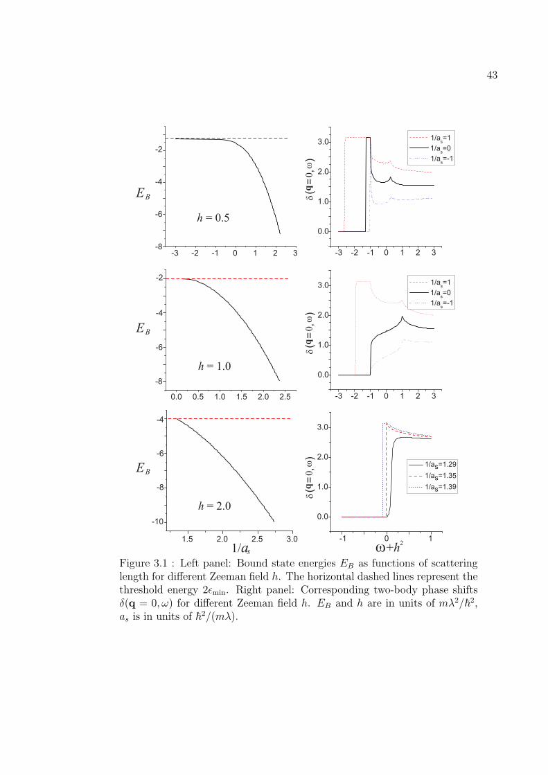
43

qω

0

ω+h2

EB

1/as

h = 0.5

h = 1.0

h = 2.0

EB

EB

qω

0q

ω0

Figure 3.1 : Left panel: Bound state energies EB as functions of scatteringlength for different Zeeman field h. The horizontal dashed lines represent thethreshold energy 2ϵmin. Right panel: Corresponding two-body phase shiftsδ(q = 0, ω) for different Zeeman field h. EB and h are in units of mλ2/~2,as is in units of ~2/(mλ).

44

We solve Eq. (3.26) numerically to find EB and the results are shown in the left

panel of Fig. 3.1, where we plot EB as a function of the contact interaction strength

for three different values of the Zeeman field (h = 0.5, 1.0 and 2.0mλ2/~2). For

h < mλ2/~2, i.e., when the Rashba ring exists as the lowest single-particle state [see

Eq. (3.21)], we always find one bound state solution regardless of the sign of as. It

is well known that, in the absence of the SO coupling, a two-body bound state does

not exist on the BCS side (i.e., as < 0). The existence of the Rashba ring induced

by the SO coupling enhances the density of states near the single-particle ground

state and favors the formation of a bound state [90]. By contrast, for h ≥ mλ2/~2,

the Rashba ring collapses to a point and a two-body bound state only occurs on the

BEC side. Furthermore, the larger the h is, the stronger attractive interaction (i.e.,

larger a−1s ) is required to have a bound state. For example, at h = 1.0mλ2/~2, the

bound state exists for a−1s > 0; at h = 2.0mλ2/~2, the bound state exists only for

a−1s > 1.35mλ/~2 (see Fig. 3.1).

A bound state can be examined by calculating the phase shift [29, 108]

δ(q, ω) = − Imln[−Γ−1

2b (q, iνn → ω + i0+)]. (3.28)

In the right panel of Fig. 3.1, we display the phase shift at q = 0. When a bound

state occurs, the phase shift will have a discontinuous jump of π when the frequency

is equal to the corresponding bound state energy as can be seen in the figure. When

the frequency is larger than 2ϵmin the molecular bound state breaks and the phase

shift comes from the usual atom atom scattering. The phase shift calculation via

Eq. (3.28) and the bound state energy calculation via Eq. (3.26) thus corroborate

each other.

45

h = 0.0

h = 0.5

h = 1.0

1/as

Figure 3.2 : Effective mass γ ≡ M⊥/(2m) as functions of scattering lengthfor different Zeeman field h. h is in units of mλ2/~2, and as is in units of~2/(mλ). For h ≥ 1, the two-body bound state only exists for as > 0.

3.3.2 Effective Mass

An important quantity that characterizes the properties of the bound state is its

effective mass. At small momentum |q|, we may assume that the bound state has

a well-defined dispersion, ϵBq = ~2q2⊥/(2M⊥) + ~2q2z/(4m), where M⊥ is the effective

mass in the transverse plane. Due to the nature of the Rashba SO coupling, the

effective mass of the bound state along the z-axis is simple twice of the atomic mass

and is not affected by the spin-orbit term. For a given q, we determine ϵBq from

the equation: Re[Γ−12b

(q;ω = EB + ϵBq

)= 0]. By Taylor expanding the two-body

inverse vertex function around |q| = 0, and after some tedious but straightforward

calculation, we obtain:

1

γ≡ 2m

M⊥= 1− 4mλ2

~2Y

X, (3.29)

46

where

X =1

V

∑k

[2h2

h2 + λ2k2⊥

]1

(EB − 2ϵk)2 +

λ2k2⊥h2 + λ2k2⊥

[1

(EB − 2ϵk,+)2

+1

(EB − 2ϵk,−)2

], (3.30)

Y =1

V

∑k

λ2k2⊥ (3h2 + λ2k2⊥)

(h2 + λ2k2⊥)2

1

(EB − 2ϵk,+) (EB − 2ϵk,−)

1

(EB − 2ϵk)

− h2λ2k2⊥(h2 + λ2k2⊥)

2

1

(EB − 2ϵk)3 − λ2k2⊥(2h

2 + λ2k2⊥)

(h2 + λ2k2⊥)2[

(EB − 2ϵk)

(EB − 2ϵk,+)2 (EB − 2ϵk,−)

2

]. (3.31)

Figure 3.2 displays the effective mass M⊥ as functions of the scattering length as

for several values of the Zeeman field strength (h). M⊥ monotonically decreases as

1/as increases. In the BEC limit where as → 0+, M⊥ → 2m independent of the value

of h.

47

3.4 Results on Many-Body Problem

We now turn to the discussion of the many-body properties. Here, we only consider

the mean-field properties of the system, while the effect of fluctuations will be studied

in the future. In the mean-field level, the order parameter ∆0 is a constant and

the corresponding momentum space single-particle Green function takes the form

(k = k, iωm),

G−10 (k) =

iωm − ξk − hσz − λ(kyσx − kxσy) i∆0σy

−i∆0σy iωm + ξk + hσz − λ(kyσx + kxσy)

.

(3.32)

Plugging this into Eq. (3.9), we may obtain the thermodynamic potential as

Ω0 =1

V

∑k

(ξk −

Ek+ + Ek−

2

)− ∆2

0

U0

− kBT∑

k,α=±

ln[1 + e−Ekα/kBT

]. (3.33)

where Ek± =√ξ2k +∆2

0 + h2 + λ2k2⊥ ± 2√

(h2 + λ2k2⊥)ξ2k + h2∆2

0 is the quasi-

particle dispersion. The chemical potential and order parameter should be determined

by,

0 =∂Ω0

∂∆0

, N = −∂Ω0

∂µ,

from which we derive the gap and the number equations as follows:

1

U0

=1

V

∑k,α=±

2f(Ekα)− 1

4Ekα

[1 + α

h2√(h2 + λ2k2⊥)ξ

2k + h2∆2

0

], (3.34)

n =1

V

∑k

1 +

∑α=±

ξk[2f(Ekα)− 1]

2Ekα

[1 + α

h2 + λ2k2⊥√(h2 + λ2k2⊥)ξ

2k + h2∆2

0

].(3.35)

In the following, we will show various quantities of physical interest, obtained from

solving Eqs. (3.34) and (3.35) self-consistently. We focus on the zero-temperature

case, although Eqs. (3.34) and (3.35) are valid for finite temperatures.

48

μ/E

F

Δ0/E

F

nn

↑/

1/( )askF

h = 0h E= 1 F

h E= 2 F

1/( )askF 1/( )askF

(a) (b) ( )c

Figure 3.3 : Chemical potential µ (a), pairing gap ∆0 (b), and populationof spin-up component n↑ (c) as functions of scattering length as for differentvalues of the Zeeman field h at λkF/EF = 2. Here kF = (3π2n)1/3 andEF = ~2k2F/(2m) are the Fermi momentum and Fermi energy, respectively.

3.4.1 Chemical Potential and Gap

We show in Fig. 3.3(a) and (b) the chemical potential µ and the pairing gap ∆0,

respectively, as functions of the scattering length for different values of the Zeeman

field. Without the Zeeman field, as spin-orbit coupling increases the density of states,

it increases BCS pairing in both the BCS region and the unitarity region. With the

Zeeman field, as it can be treated as the chemical potential difference of the two

species. The bigger external Zeeman field means the more imbalanced in the system.

The Zeeman field makes BCS pairing for the k, ↑ atom different from the k, ↓ atoms

as the Fermi surfaces for the two species mismatch. It suppresses the pairing gap.

In Fig. 3.3(c), we plot the population of the spin-up component. For zero Zeeman

field, we always have equal population in both spin components. For h > 0, the

spin-up component has less population. In all cases, the effects of the Zeeman field

together with the spin orbit coupling reduce as the BEC limit (i.e., 1/as → +∞) is

approached.

49

3.4.2 Quasi-particle Spectrum

The quasi-particle dispersion Ek± is plotted in Fig. 3.4. The spectrum is sensitive

to the polar angle θ of the momentum vector k. For k along the z-axis (i.e., θ = 0

and k⊥ = 0), Ek− may become zero at certain values of k when h is sufficiently large,

signaling a gapless dispersion. The points at which Ek− = 0 are called Fermi points.

The value of the Zeeman field at which new Fermi points appear represents a quantum

critical point for topological phase transition [95, 102]. For µ > 0, the system may

support 0, 2 or 4 Fermi points along the kz-axis as h is increased. For µ < 0 which

is the case illustrated in Fig. 3.4, there can be either 0 or 2 Fermi points [96]. For

λkF/EF = 2, the critical Zeeman field is hc ≈ 1.5EF . For h < hc, the system is a

topologically trivial gapped superfluid; for h > hc, the system possesses two Fermi

points and represents a topologically nontrivial gapless superfluid. Note that the

quasi-particle dispersion has been measured in recent experiments on ultracold Fermi

gases [51, 52] using momentum resolved radio frequency spectroscopy.

3.4.3 Pairing Profile

Even though in our model the interaction has a contact s-wave form, due to the

presence of the SO coupling, pairing can occur in both singlet and triplet channels

[103]. The singlet pairing field between unlike spins can be calculated as:

⟨ψk↑ψ−k↓⟩ = −∆0

∑α=±

2f(Ekα)− 1

4Ekα

[1 + αh2√

(h2 + λ2k2⊥)ξ2k + h2∆2

0

]

,(3.36)

50

(a) (b)

Ek±

k k/ F k k/ F

Figure 3.4 : Quasi-particle dispersion spectrum Ek+ (solid lines) and Ek−(dashed lines) shown in in units of EF for k in the transverse plane (a,θ = π/2) and along the z-axis (b, θ = 0) for λkF/EF = 2, h/EF = 2.

while the triplet pairing fields between like spins are given by:

⟨ψk↑ψ−k↑⟩ = ∆0λ(ky + ikx)(ξk − h)√(h2 + λ2k2⊥)ξ

2k + h2∆2

0

[2f(Ek+)− 1

4Ek+

− 2f(Ek−)− 1

4Ek−

],(3.37)

⟨ψk↓ψ−k↓⟩ = −∆0λ(ky − ikx)(ξk + h)√(h2 + λ2k2⊥)ξ

2k + h2∆2

0

[2f(Ek+)− 1

4Ek+

− 2f(Ek−)− 1

4Ek−

].(3.38)

We plot in Fig. 3.5 the absolute value of the various pairing fields. One can see

that the effect of the Zeeman field is to reduce the singlet pairing while enhancing

the triplet pairing.

3.4.4 Density of States

From the single-particle Green’s function, one can immediately obtain the density of

states which is an important quantity characterizing the nature of the quantum state.

51

kk

z/

F

k k/ F

ψ ψk -k

ψ ψ¯k -k

ψ ψ¯ ¯k -k

0

0.25

0.50

↑ ↑ ↑

Figure 3.5 : Pairing fields at unitarity (i.e., 1/as = 0) for h = 0 (top row),h = 1EF (middle row), h = 2EF (bottom row) and λkF/EF = 2. In eachrow, from left to right, we display |⟨ψk↑ψ−k↓⟩|, |⟨ψk↑ψ−k↑⟩| and |⟨ψk↓ψ−k↓⟩|(all in units of EF ), respectively.

52

We invert Eq. (3.32) to get

G0 (k, iωm) =

g(k, iωm) f(k, iωm)[f(+k,−iωm)

]+− [g(−k,−iωm)]T

, (3.39)

where g and f are both 2× 2 matrices whose expressions are.

g(k, iωm) = [iωm + ξk − hσz + λ(kyσx − kxσy)]D+/M,

f(k, iωm) = [−i∆0σy]D−/M. (3.40)

with

M =[(iωm − h)2 − ξ2k −∆2

0 − λ2k2⊥] [

(iωm + h)2 − ξ2k −∆20 − λ2k2⊥

]−4λ2k2⊥

(ξ2k − h2

),

(3.41)

and

D+ =

(iωm + h)2 − ξ2k −∆20 − λ2k2⊥ λ (ky + ikx) [2 (ξk + h)]

λ (ky − ikx) [2 (ξk − h)] (iωm − h)2 − ξ2k −∆20 − λ2k2⊥

,(3.42)D− =

(iωm − h)2 − ξ2k −∆20 − λ2k2⊥ −λ (ky − ikx) [2 (ξk + h)]

−λ (ky + ikx) [2 (ξk − h)] (iωm + h)2 − ξ2k −∆20 − λ2k2⊥

.(3.43)In greater detail, we find that,

g(k, iωm) =

g11 (k, iωm) g12 (k, iωm)

g∗12 (k,−iωm) g22 (k, iωm)

, (3.44)

where,

Mg11 (k, iωm) = [iωm + ξk − h][(iωm + h)2 − ξ2k −∆2

0 − λ2k2⊥]

+2λ2k2⊥ (ξk − h) , (3.45)

Mg12 (k, iωm) = λ (ky + ikx)[(iωm + ξk)

2 − h2 −∆20 − λ2k2⊥

], (3.46)

Mg22 (k, iωm) = [iωm + ξk + h][(iωm − h)2 − ξ2k −∆2

0 − λ2k2⊥]

+2λ2k2⊥ (ξk + h) , (3.47)

53

ω/EF

h = 0h E= 1 F

h E= 2 F

(a) (b)

ρ↑ ρ

↓

ω/EF

Figure 3.6 : Density of states ρ↑ (a) and ρ↓ (b) at unitarity and λkF/EF = 2.

and

f(k, iωm) =∆0

M

λ (ky + ikx) [2 (ξk − h)] −[(iωm + h)2 − ξ2k −∆2

0 − λ2k2⊥]

[(iωm − h)2 − ξ2k −∆2

0 − λ2k2⊥]

−λ (ky − ikx) [2 (ξk + h)]

.(3.48)

The density of states are related to the g matrix as

ρ↑(ω) = − 1

πIm

[1

V

∑k

g11(k, ω + i0+)

], (3.49)

ρ↓(ω) = − 1

πIm

[1

V

∑k

g22(k, ω + i0+)

]. (3.50)

where the expressions of g11 and g22 can be found in Eqs. (3.45) and (3.47).

We show in Fig. 3.6 the density of states at different Zeeman fields. At h = 0,

ρ↑ and ρ↓ are identical, both exhibiting a large gapped region. As h increases, the

gapped region shrinks. Furthermore, the density of states for the majority component

(which is the spin down component for our choice of positive h) becomes more V-

shaped near ω = 0 when there are Fermi points in the spectrum. A V-shaped density

of states comes from the node of the pairing which is the characteristic feature of

many unconventional superconductors with non-s-wave pairing. Here it is due to the

54

pairing resulting from the SO coupling together with the Zeeman field. The density

of states may be measured in experiment using the scheme proposed in Ref. [109].

3.4.5 Spin Structure Factor

Finally, let us consider the spin structure factor [58, 60] which is related to the dynamic

spin susceptibility χS (q, iνn), which is the Fourier transformation of the spin-spin

correlation function

χS (x, τ) = −⟨TτδnS (x, τ) δnS (0, 0)⟩ . (3.51)

where the spin density is given by δnS = n↑ − n↓. Using the Nambu spinor notation,

the spin density can be written as,

δnS =1

2Φ+

1 0 0 0

0 −1 0 0

0 0 −1 0

0 0 0 1

Φ =

1

2Φ+ [τz ⊗ σz] Φ. (3.52)

where τi are the Pauli matrices describing the Nambu spinor degrees of freedom.

Within the static Bogoliubov approximation, we have,

χS (q, iνn) =1

4kBT

∑k,iωm

Tr τz ⊗ σzG0 (k, iωm) τz ⊗ σzG0 (k+ q, iωm + iνn) .

(3.53)

The zero-momentum dynamic spin structure factor is given by

SS (q = 0, ω) = − 1

1− e−ω/kBT1

πIm[χS(q = 0, iνn → ω + i0+

)], (3.54)

via analytic continuation and the fluctuation-dissipation theorem.

Here we only consider the zero temperature case.

55

χs(0, ivn) =1

2

1

βV

∑k,iwn

g11(k, iwn)g11(k, iwn + ivn)− g12(k, iwn)g21(k, iwn + ivn)

−g21(k, iwn)g12(k, iwn + ivn) + g22(k, iwn)g22(k, iwn + ivn)

−f11(k, iwn)f∗11(k,−iwn − ivn) + f12(k, iwn)f

∗12(k,−iwn − ivn)

+f21(k, iwn)f∗21(k,−iwn − ivn)− f22(k, iwn)f

∗22(k,−iwn − ivn)(3.55)

Ss(0, w) =1

16

1

V

∑k

δ(w − 2Ek+)[u011(k+)v

011(k+) + u111(k+)v

111(k+)

−u12(k+)v12(k+)− p2+(k) + q2(k) +∆2(ζ2k + h2)λ2k2⊥

[(h2 + λ2k2⊥)ζ2k + h2∆2]E2

k+

]

+1

16

1

V

∑k

δ(w − 2Ek−)[u011(k−)v

011(k−) + u111(k−)v

111(k−)

−u12(k−)v12(k−)− p2−(k) + q2(k) +∆2(ζ2k + h2)λ2k2⊥

[(h2 + λ2k2⊥)ζ2k + h2∆2]E2

k−]

−v12(k+)v12(k−) + 2p+(k)p−(k)− 2q2(k) +2∆2(ζ2k + h2)λ2k2⊥

[(h2 + λ2k2⊥)ζ2k + h2∆2]Ek+Ek−

]

+1

16

1

V

∑k

δ(w − Ek+ − Ek−)[u011(k+)v

011(k−) + v011(k+)u

011(k−)

+u111(k+)v111(k−) + v111(k+)u

111(k−)− u12(k+)v12(k−)− v12(k+)u12(k−)

−2p+(k)p−(k)− 2q2(k)− 2∆2(ζ2k + h2)λ2k2⊥[(h2 + λ2k2⊥)ζ

2k + h2∆2]Ek+Ek−

] (3.56)

where

u011(k+) = 1 +ζkEk+

+ζk(h

2 + λ2k2⊥)

Ek+√

(h2 + λ2k2⊥)ζ2k + h2∆2

v011(k+) = 1− ζkEk+

− ζk(h2 + λ2k2⊥)

Ek+√

(h2 + λ2k2⊥)ζ2k + h2∆2

u011(k−) = 1 +ζkEk−

− ζk(h2 + λ2k2⊥)

Ek−√(h2 + λ2k2⊥)ζ

2k + h2∆2

v011(k−) = 1− ζkEk−

+ζk(h

2 + λ2k2⊥)

Ek−√(h2 + λ2k2⊥)ζ

2k + h2∆2

(3.57)

56

u111(k+) =h

Ek++

ζkh√(h2 + λ2k2⊥)ζ

2k + h2∆2

+h(ζ2k +∆2)

Ek+√

(h2 + λ2k2⊥)ζ2k + h2∆2

v111(k+) = − h

Ek++

ζkh√(h2 + λ2k2⊥)ζ

2k + h2∆2

− h(ζ2k +∆2)

Ek+√

(h2 + λ2k2⊥)ζ2k + h2∆2

u111(k−) =h

Ek−− ζkh√

(h2 + λ2k2⊥)ζ2k + h2∆2

− h(ζ2k +∆2)

Ek−√(h2 + λ2k2⊥)ζ

2k + h2∆2

v111(k−) = − h

Ek−− ζkh√

(h2 + λ2k2⊥)ζ2k + h2∆2

+h(ζ2k +∆2)

Ek−√

(h2 + λ2k2⊥)ζ2k + h2∆2

(3.58)

u12(k+) =λk⊥Ek+

[1 +ζk(ζk + Ek+)√

(h2 + λ2k2⊥)ζ2k + h2∆2

]

v12(k+) = −λk⊥Ek+

[1 +ζk(ζk − Ek+)√

(h2 + λ2k2⊥)ζ2k + h2∆2

]

u12(k−) =λk⊥Ek−

[1− ζk(ζk + Ek−)√(h2 + λ2k2⊥)ζ

2k + h2∆2

]

v12(k−) = −λk⊥Ek−

[1− ζk(ζk − Ek−)√(h2 + λ2k2⊥)ζ

2k + h2∆2

] (3.59)

p+(k) = − ∆

Ek+[1 +

h2√(h2 + λ2k2⊥)ζ

2k + h2∆2

]

p−(k) = − ∆

Ek−[1− h2√

(h2 + λ2k2⊥)ζ2k + h2∆2

]

q(k) = − h∆√(h2 + λ2k2⊥)ζ

2k + h2∆2

(3.60)

It can be explicitly shown that the dynamic spin structure factor vanishes when

λ = 0, i.e., in the absence of the SO coupling. Hence a nonzero spin structure factor is

a direct consequence of triplet pairing. Fig. 3.7(a) shows the dynamic spin structure

factor at different Zeeman fields. At h = 0, SS(0, ω) exhibits a broad peak. For finite

h, an additional narrower peak appears at smaller energy. The corresponding static

57

ω/EF

h = 0h E= 1 F

h E= 2 F

Ss(0

,)

ω

λkF/EF

Ss(0

)

h = 0h E= 0.25 F

h E= 0.5 F

(a) (b)

Figure 3.7 : (a) Zero temperature dynamic spin structure factor SS(0, ω) atunitarity and λkF/EF = 2. (b) Static spin structure factor SS(0) as functionsof the SO coupling strength.

spin structure factor is given by

SS(0) =

∫dω SS(0, ω) ,

which is plotted in Fig. 3.7(b) as a function of the SO coupling strength. The spin

structure factor may be directly measured in experiments using the Bragg spectro-

scopic method [61, 62, 63].

58

Chapter 4

Single Impurity In Ultracold Fermi Superfluids

4.1 Model

The development of ultracold atoms provide us with selective experimental controls

of many-body quantum system. In ultracold atoms, both the sign and value of the

interaction can be accurately tuned using laser lights or magnetic fields. This shows

a great advantage compared with the conventional quantum many-body system such

as a condensed matter system. In condensed matter experiments, one big problem is

the defects contained in the material. The defect comes so naturally in experiments

people almost can not avoid them. The only way is to understand the physics of

defects in many-body problems. Then comes the theory for impurities in many-

body system, which turns out to be a great treasure in condensed matter physics.

Impurities can be used as the detector of quantum effects [110, 111]. Single impurities

have been employed in the detection of superconducting pairing symmetry within

unconventional superconductors [112] and to demonstrate Friedel oscillations [113]. In

strongly correlated systems, they may be used to pin one of the competing orders [114].

Even though cold atom systems are intrinsically clean, the effects of impurities may

be simulated by employing laser speckles or quasiperiodic lattices [115]. Controllable

manipulation of individual impurities in cold atom systems can also be realized using

off-resonant laser light or another species of atoms/ions [116, 117, 118, 119]. With

some notable advantages in cold atom systems, we anticipate important contributions

59

for cold atom systems from the study of impurities. Such impurities can be either

localized or extended and either static or dynamic. The unprecedented access to

accurately tune these artificial impurities provides an exciting possibility to probe

and manipulate the properties of cold atoms.

In this chapter, we demonstrate this possibility using a single classical static impu-

rity in an s-wave Fermi superfluid. By ‘classical’ we refer to the treatment of the im-

purity as a scattering potential which has no internal degrees of freedom. We focus on

both a single non-magnetic impurity and a magnetic impurity. For the non-magnetic

impurity, it scatters each spin species equally while for the magnetic impurity it

scatters differently. We study both a local impurity and an extended impurity in

one-dimension(1D) and three-dimensions(3D). From our self-consistent Bogoliubov-

de Gennes calculations we show for the first time in a trapped three-dimensional ge-

ometry that the long sought Fulde-Ferrell-Larkin-Ovchinnikov (FFLO) phase, which

supports many mid-gap bound states, may be induced through such an impurity at

experimentally accessible parameters. Furthermore, we propose that these bound

states can be probed using a modified radio-frequency (RF) spectroscopy technique

that is the analog of the widely used scanning tunneling microscope (STM) in solid

state and that this can serve as a powerful general tool in probing and manipulating

quantum gases.

For computational simplicity, we first focus on a one-dimensional system and verify

the essential physics at higher dimensions in later paragraphs. Consider the following

Hamiltonian at zero temperature,

H =∑σ=↑,↓

∫dxψ†

σ

[− ~2

2m

d2

dx2− µσ + VT

]ψσ

+g

∫dxψ†

↑ψ†↓ψ↓ψ↑ +

∑σ=↑,↓

∫dxψ†

σUσψσ, (4.1)

60

where ψ†σ(x) and ψσ(x) are, respectively, the fermionic creation and annihilation oper-

ators for spin species σ. VT (x) is a harmonic trapping potential and g is the strength

of the inter-atomic interaction. In this work, we take g to be small and negative so

that the system is a superfluid at low temperatures and, as for theory, mean field cal-

culation is still valid in the weak interaction case. The last term of the Hamiltonian

describes the effect of the impurity which is represented by a scattering potential,

Uσ(x). For a non-magnetic impurity, U↑(x) = U↓(x); while for a magnetic impurity,

U↑(x) = −U↓(x). Note that a general impurity potential can be decomposed into a

sum of magnetic and non-magnetic parts. Here we focus on both non-magnetic and

magnetic impurities which can be either localized or extended.

In the next two sections, I will introduce two methods to treat the impurity

problem.

61

4.2 T-Matrix Method

The T-Matrix for single impurity is a perturbation theory. It describes multiple

scattering process between an atom and an impurity. It is an exact method for a

single impurity as it covers all the diagrams. It is analytically solvable when the

perturbation term is independent of momentum k. For the localized impurity which

can be described as a contact impurity, The T-matrix method is an exact solvable

method[120, 121].

The Hamiltonian for a contact impurity in an s-wave superfluid can be written in

momentum space as:

H = H0 +W =∑k,σ

ξkc+k,σck,σ +

∑k

(∆c+k,↑c+−k,↓ + h.c.)

+u

V

∑k,q

c+k+q,σck,σ (4.2)

Here c+k,σ is a fermion creation operator for a ”spin σ” atom, ck,σ is a fermion an-

nihilation operator for a ”spin σ” atom. W = uV

∑k,q c

+k+q,σck,σ represents the im-

purity potential which is∫drU(r)ψ+(r)ψ(r) and when U(r) is a contact potential

U(r) = uδ(r). We assume the impurity is located at the origin. We consider the

definition of the Green’s Function:

G(iwn) =1

iwn −H=

1

iwn −H0 −W

=1

G0(iwn)−1 −W(4.3)

Here W is just like the self-energy in the interaction case as we can treat the self-

energy as an external field. This is just Dyson’s equation. We can rewrite the form

62

as a series expansion and get:

G(iwn) = G0(iwn) +G0(iwn)WG(iwn)

= G0(iwn) +G0(iwn)WG0(iwn)

+G0(iwn)WG0(iwn)WG0(iwn) + ... (4.4)

In the momentum basis, we have

G(k,k′, iwn) = ⟨k|G(iwn)|k′⟩

= G0(k, iwn)δk,k′ +G0(k, iwn)u

VG0(k

′, iwn)

+G0(k, iwn)u

V

∑k1

G0(k1, iwn)u

VG0(k

′, iwn) + ...

= G0(k, iwn)δk,k′ +1

VG0(k, iwn)T (iwn)G0(k

′, iwn) (4.5)

Here, as the impurity breaks translational symmetry, the system is no longer homo-

geneous. The Green’s function will have two momentum labels k, k′.

Let us define the T-matrix as:

T (iwn) = u+ u∑k1

G0(k1, iwn)u

V+ u[

∑k1

G0(k1, iwn)u

V]2 + ...

=u

1−∑k1

G0(k1, iwn)uV

(4.6)

Due to the use of a contact impurity, the T-matrix can be written as the sum of

a geometric series and is independent of momentum. This greatly simplifies the

calculation and in this way we can evaluate the T-matrix analytically.

T (iwn)−1 = u−1 −G0(0, iw) (4.7)

where:

G0(r, iw) =1

V

∑k1

eik1rG0(k1, iw) (4.8)

63

G0(r, iw) is the Green’s function for a homogeneous system in real space. For the

Green’s function for an inhomogeneous system in real space, we get

G(r, r, iw) =1

V

∑k,k′

eikr−ik′rG(k,k′, iw)

= G0(0, iw) +G0(r, iw)T (iw)G0(−r, iw) (4.9)

from which we can calculate the local density of states(LDOS):

ρ(r, E) = − 1

πImG(r, r, E + i0+) (4.10)

For the superfluid phase, we write the BCS mean field Hamiltonian in Nambu

notation as a 2× 2 matrix:

H = H0 +W

=∑k

(c+k↑, c−k↓)

ϵ(k) ∆(k)

∆(k)∗ −ϵ(k)

( ck↑c+−k↓

)

+1

V

∑k,k′

(c+k↑, c−k↓)

u 0

0 −u

( ck′↑

c+−k′↓

)(4.11)

Here we introduce the Nambu spinor: (c+k↑, c−k↓). The impurity potential here is

non-magnetic and has the form of uτ3. For a magnetic impurity, it has the form of

uτ0.

Let us define the matrix Green’s function as:

G(k,k, τ) = −⟨Tτ

ck↑(τ)c+k↑(0) ck↑(τ)c−k↓(0)

c+−k↓(τ)c+k↑(0) c+−k↓(τ)c−k↓(0)

⟩ (4.12)

We are interested in the local density of states, which is given by

ρ(r, E) = − 1

πImG11(r, r, E + i0+) +

1

πImG22(r, r,−E − i0+) (4.13)

64

Where the first term corresponds to the local density of states for spin up atoms and

the second term for spin down atoms. Since the local density of states is independent

of spin directions in the balanced case with non-magnetic impurities, we have:

− 1

πImG11(r, r, E + i0+) =

1

πImG22(r, r,−E − i0+) (4.14)

We now calculate the unperturbed Green’s function:

G0(k, iwn) = ⟨k| 1

iwn −H0

|k⟩ =

iwn − ξk −∆

−∆∗ iwn + ξk

−1

=1

(iwn)2 − ξ2k −∆

iwn + ξk ∆

∆∗ iwn − ξk

(4.15)

The T matrix is

T (iwn) = uτ3 + uτ3G0(0, iwn)uτ3 + uτ3G0(0, iwn)uτ3

G0(0, iwn)uτ3 + · · ·

= uτ3 + uτ3G0(0, iwn)T (iwn)

= (1− uτ3G0(0, iwn))−1uτ3 (4.16)

So

T−1(iwn) =1

uτ3(1− uτ3G0(0, iwn))

=1

uτ3 −G0(0, iwn) (4.17)

where

G0(0, iwn) =1

V

∑k

G0(k, iwn)

=

1V

∑k

iwn+ξk(iwn)2−ξ2k−∆2

1V

∑k

∆(iwn)2−ξ2k−∆2

1V

∑k

∆∗

(iwn)2−ξ2k−∆21V

∑k

iwn−ξk(iwn)2−ξ2k−∆2

(4.18)

65

So the inverse of the T-matrix can be written as

T−1(iwn) =

1u− 1

V

∑k

iwn+ξk(iwn)2−ξ2k−∆2 − 1

V

∑k

∆(iwn)2−ξ2k−∆2

− 1V

∑k

∆∗

(iwn)2−ξ2k−∆2 − 1u− 1

V

∑k

iwn−ξk(iwn)2−ξ2k−∆2

(4.19)

The problem now is to do the integral. This can be analytically calculated using a

contour integral. Here I show the results for the 1D superfluid. The results for 3D are

similar. As for the BEC-BCS crossover, the chemical potential can be both positive

and negative. We have to divide the integral into many cases.

Case 1. when |w| < ∆

We can define ϵ =√−w2 +∆2

We find that all the imaginary parts are zero. This is true because here we are

considering s-wave pairing which does not have nodes. Inside the gap, the imaginary

part of Green’s function should be zero.

Case 1.1 when µ > 0

ReG0(0, w + i0+)11 = −(ϵ+ w) cos(1

2arctan(µ

ϵ))− (ϵ− w) sin(1

2arctan(µ

ϵ))

2√2ϵ(ϵ2 + µ2)1/4

(4.20)

ReG0(0, w + i0+)12 = −∆[√ϵµ(ϵ+

√ϵ2 + µ2) + (ϵ2 + µ2)1/4

√ϵµ3

µ2+ϵ(ϵ+√ϵ2+µ2)

]

4√ϵ3µ(ϵ2 + µ2)

(4.21)

ReG0(0, w + i0+)22 =(ϵ− w) cos(1

2arctan(µ

ϵ))− (ϵ+ w) sin(1

2arctan(µ

ϵ))

2√2ϵ(ϵ2 + µ2)1/4

(4.22)

Case 1.2 when µ < 0

ReG0(0, w + i0+)11 = −1

2

√−µ+

√ϵ2 + µ2

2(ϵ2 + µ2)+w sin[1

2arctan( ϵ

µ)]

2ϵ(ϵ2 + µ2)1/4(4.23)

ReG0(0, w + i0+)12 =∆sin[1

2arctan( ϵ

µ)]

2ϵ(ϵ2 + µ2)1/4(4.24)

ReG0(0, w + i0+)22 =1

2

√−µ+

√ϵ2 + µ2

2(ϵ2 + µ2)+w sin[1

2arctan( ϵ

µ)]

2ϵ(ϵ2 + µ2)1/4(4.25)

66

Case 2. when |w| > ∆

Define ε± = ±√w2 −∆2

For imaginary parts, we have to deal with the delta function using

δ(f(x)) =∑i

δ(x− xi)

|f ′(xi)|(4.26)

where the xi are roots for f(x) = 0. We get

Case 2.1 when −µ > ε+

The imaginary parts are zero.

ReG0(0, w + i0+)11 = −ε+(

1√−ε+−µ + 1√

ε+−µ) + w( 1√−ε+−µ − 1√

ε+−µ)

4ε+(4.27)

ReG0(0, w + i0+)12 =∆(

√−ε+ − µ−

√ε+ − µ)

4ε+√

−ε2+ + µ2(4.28)

ReG0(0, w + i0+)22 =ε+(

1√−ε+−µ + 1√

ε+−µ) + w(− 1√−ε+−µ + 1√

ε+−µ)

4ε+(4.29)

Case 2.2 when ε− < −µ < ε+

ReG0(0, w + i0+)11 =−ε+ + w

4ε+√ε+ − µ

(4.30)

ReG0(0, w + i0+)12 =∆

4ε+√ε+ − µ

(4.31)

ReG0(0, w + i0+)22 =ε+ + w

4ε+√ε+ − µ

(4.32)

when w < 0

ImG0(0, w + i0+)11 =1√

ε+ + µ

w + ε+4ε+

(4.33)

ImG0(0, w + i0+)12 =1√

ε+ + µ

∆

4ε+(4.34)

ImG0(0, w + i0+)22 =1√

ε+ + µ

w − ε+4ε+

(4.35)

67

when w > 0

ImG0(0, w + i0+)11 = − 1√ε+ + µ

w + ε+4ε+

(4.36)

ImG0(0, w + i0+)12 = − 1√ε+ + µ

∆

4ε+(4.37)

ImG0(0, w + i0+)22 = − 1√ε+ + µ

w − ε+4ε+

(4.38)

Case 2.3 when −µ < ε−

All the real parts are zero.

when w < 0

ImG0(0, w + i0+)11 =1√

ε+ + µ

w + ε+4ε+

+1√

−ε+ + µ

w − ε+4ε+

(4.39)

ImG0(0, w + i0+)12 =1√

ε+ + µ

∆

4ε++

1√−ε+ + µ

∆

4ε+(4.40)

ImG0(0, w + i0+)22 =1√

ε+ + µ

w − ε+4ε+

+1√

−ε+ + µ

w + ε+4ε+

(4.41)

when w > 0

ImG0(0, w + i0+)11 = − 1√ε+ + µ

w + ε+4ε+

− 1√−ε+ + µ

w − ε+4ε+

(4.42)

ImG0(0, w + i0+)12 = − 1√ε+ + µ

∆

4ε+− 1√

−ε+ + µ

∆

4ε+(4.43)

ImG0(0, w + i0+)22 = − 1√ε+ + µ

w − ε+4ε+

− 1√−ε+ + µ

w + ε+4ε+

(4.44)

With all these we can first get the inverse of T-matrix. Then by using the form

for Green’s function, we can get Green’s function at the impurity point. Using the

T-matrix method we can get analytical results. This T-matrix method can only solve

analytically for the case of a contact impurity. For a more general impurity, we need

a more efficient method, that is, the Bogoliubov-de Gennes(B-dG) method.

68

4.3 The Hybrid Bogoliubov-de Gennes Method

The Bogoliubov-de Gennes(B-dG) method is a powerful tool to calculate the pairing

gap and other physical properties for inhomogeneous systems[122, 123, 124, 125, 126].

It is extremely useful in cold atoms as the system is in the trap. Here I derive the

hybrid B-dG method which deals with the renormalization and is more efficient. This

method introduces an energy cut-off Ec in the calculation. Below the cut-off, it uses

the standard B-dG to discretize the system; above the cut-off, it uses the local density

approximation(LDA) to solve the system continuously. In this chapter, we use the

B-dG method to treat both a localized impurity and an extended impurity.

4.3.1 Below Cut-off: Bogoliubov-de Gennes Method

As we will introduce the magnetic impurity, it breaks population balance in the

system. The chemical potentials are different for different species.

We start from the the Hamiltonian

H =∑σ

∫drψ+

σ (r)[−~2∇2

2m− µσ − V (r)]ψσ(r)

+g

∫drψ+

↑ (r)ψ+↓ (r)ψ↓(r)ψ↑(r) (4.45)

where ψ+σ is Fermion creation operator for ”spin σ” atom, ψσ is Fermion annihilation

operator for ”spin σ” atom, g is the contact interaction strength.

We treat this first part as H0, H = H0 + V . We use the set of eigenstates η for

H0, then the first part can be written as:

H0 =∑η,σ

ε0ησc+ησcησ (4.46)

where ψσ(r) =∑η

⟨r|η⟩cησ. In a cold atom system, the basis set is the one for the

harmonic trap potential.

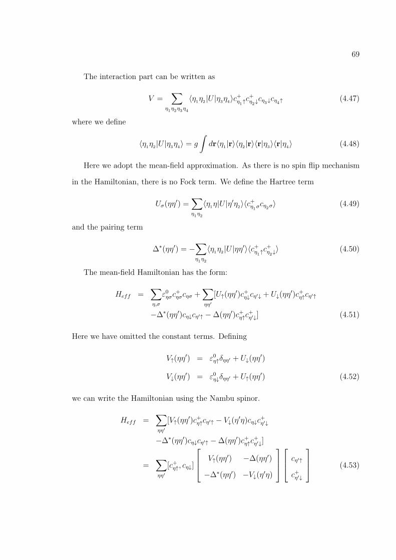
69

The interaction part can be written as

V =∑

η1η2η3η4

⟨η1η2 |U |η3η4⟩c+η1↑c+η2↓cη3↓cη4↑ (4.47)

where we define

⟨η1η2 |U |η3η4⟩ = g

∫dr⟨η1 |r⟩⟨η2 |r⟩⟨r|η3⟩⟨r|η4⟩ (4.48)

Here we adopt the mean-field approximation. As there is no spin flip mechanism

in the Hamiltonian, there is no Fock term. We define the Hartree term

Uσ(ηη′) =

∑η1η2

⟨η1η|U |η′η2⟩⟨c+η1σcη2σ⟩ (4.49)

and the pairing term

∆∗(ηη′) = −∑η1η2

⟨η1η2 |U |ηη′⟩⟨c+η1↑c+η2↓

⟩ (4.50)

The mean-field Hamiltonian has the form:

Heff =∑η,σ

ε0ησc+ησcησ +

∑ηη′

[U↑(ηη′)c+η↓cη′↓ + U↓(ηη

′)c+η↑cη′↑

−∆∗(ηη′)cη↓cη′↑ −∆(ηη′)c+η↑c+η′↓] (4.51)

Here we have omitted the constant terms. Defining

V↑(ηη′) = ε0η↑δηη′ + U↓(ηη

′)

V↓(ηη′) = ε0η↓δηη′ + U↑(ηη

′) (4.52)

we can write the Hamiltonian using the Nambu spinor.

Heff =∑ηη′

[V↑(ηη′)c+η↑cη′↑ − V↓(η

′η)cη↓c+η′↓

−∆∗(ηη′)cη↓cη′↑ −∆(ηη′)c+η↑c+η′↓]

=∑ηη′

[c+η↑, cη↓]

V↑(ηη′) −∆(ηη′)

−∆∗(ηη′) −V↓(η′η)

cη′↑

c+η′↓

(4.53)

70

We need to diagonalize this matrix, but first we need a cut-off for the system. Say

we only consider the lowest N There are 2N eigenvalues. The maximum(minimum)

value should be equal to the cut-off energy Ec(In real numerical calculations, due to

the computational accuracy, we usually diagonalize a much larger matrix, and only

consider states with energy less than cut-off energy).

To diagonalize the matrix, we introduce a unitary transform U .

Heff =∑

ηη′=1,N

[c+η↑, cη↓]UU+

V↑(ηη′) −∆(ηη′)

−∆∗(ηη′) −V↓(η′η)

UU+

cη′↑

c+η′↓

(4.54)

Assume V↑(ηη′) −∆(ηη′)

−∆∗(ηη′) −V↓(η′η)

2N×2N

uη′

vη′

2N×1

= E

uη

vη

2N×1

(4.55)

where E is eigenvalue, uη′ , vη′ are eigenstates with∑η′(|uη′ |2 + |vη′|2) = 1. It has 2N

sets of eigenvalues and eigenstates. Defining the unitary matrix:

U =

uηn

vηn

(4.56)

where η = 1, ...N , n = 1, ...2N .

U+ = [u∗nη, v∗nη] (4.57)

We have γη↑

γ+η↓

= U+

cη↑

c+η↓

(4.58)

(4.59)

71

We get

cη↑ =∑n=1,N

uηnγn↑ +∑n=1,N

uη,N+nγ+n↓

c+η↑ =∑n=1,N

u∗ηnγ+n↑ +

∑n=1,N

u∗η,N+nγn↓

c+η↓ =∑n=1,N

vηnγn↑ +∑n=1,N

vη,N+nγ+n↓

cη↓ =∑n=1,N

v∗ηnγ+n↑ +

∑n=1,N

v∗η,N+nγn↓ (4.60)

The mean-field Hamiltonian can be diagonalized

Heff =∑ηη′

[γ+η↑, γη↓]

· 0 0

0 E 0

0 0 ·

γη′↑

γ+η′↓

=

∑η=1,N

Eηγ+η↑γη↑ −

∑η=1,N

EN+ηγ+η↓γη↓ (4.61)

Now we derive the density profile for different species.

⟨n↑(x)⟩ =∑

n=1,2N

(∑η

⟨η|x⟩u∗ηn)(∑η′

⟨x|η′⟩uη′n)f(En) (4.62)

⟨n↓(x)⟩ =∑

n=1,2N

(∑η

⟨η|x⟩vηn)(∑η′

⟨x|η′⟩v∗η′n)f(−En) (4.63)

The gap profile is

∆(x) = −g∑

n=1,2N

(∑η

⟨x|η⟩v∗ηn)(∑η′

⟨x|η′⟩uη′n)f(En) (4.64)

and the local density of states(LDOS) is given by

ρ↑(r, iwn → w + i0+) =∑η,η′

⟨r|η⟩⟨η′|r⟩∑

n=1,2N

uηnu∗η′nδ(w − En) (4.65)

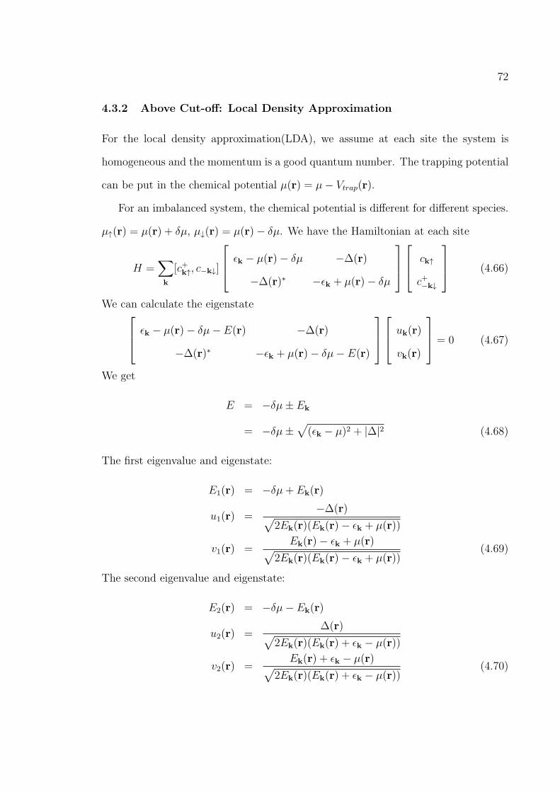
72

4.3.2 Above Cut-off: Local Density Approximation

For the local density approximation(LDA), we assume at each site the system is

homogeneous and the momentum is a good quantum number. The trapping potential

can be put in the chemical potential µ(r) = µ− Vtrap(r).

For an imbalanced system, the chemical potential is different for different species.

µ↑(r) = µ(r) + δµ, µ↓(r) = µ(r)− δµ. We have the Hamiltonian at each site

H =∑k

[c+k↑, c−k↓]

ϵk − µ(r)− δµ −∆(r)

−∆(r)∗ −ϵk + µ(r)− δµ

ck↑

c+−k↓

(4.66)

We can calculate the eigenstate ϵk − µ(r)− δµ− E(r) −∆(r)

−∆(r)∗ −ϵk + µ(r)− δµ− E(r)

uk(r)

vk(r)

= 0 (4.67)

We get

E = −δµ± Ek

= −δµ±√(ϵk − µ)2 + |∆|2 (4.68)

The first eigenvalue and eigenstate:

E1(r) = −δµ+ Ek(r)

u1(r) =−∆(r)√

2Ek(r)(Ek(r)− ϵk + µ(r))

v1(r) =Ek(r)− ϵk + µ(r)√

2Ek(r)(Ek(r)− ϵk + µ(r))(4.69)

The second eigenvalue and eigenstate:

E2(r) = −δµ− Ek(r)

u2(r) =∆(r)√

2Ek(r)(Ek(r) + ϵk − µ(r))

v2(r) =Ek(r) + ϵk − µ(r)√

2Ek(r)(Ek(r) + ϵk − µ(r))(4.70)

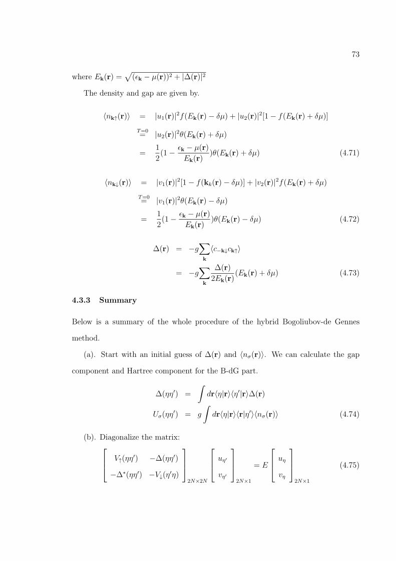
73

where Ek(r) =√(ϵk − µ(r))2 + |∆(r)|2

The density and gap are given by.

⟨nk↑(r)⟩ = |u1(r)|2f(Ek(r)− δµ) + |u2(r)|2[1− f(Ek(r) + δµ)]

T=0= |u2(r)|2θ(Ek(r) + δµ)

=1

2(1− ϵk − µ(r)

Ek(r))θ(Ek(r) + δµ) (4.71)

⟨nk↓(r)⟩ = |v1(r)|2[1− f(kk(r)− δµ)] + |v2(r)|2f(Ek(r) + δµ)

T=0= |v1(r)|2θ(Ek(r)− δµ)

=1

2(1− ϵk − µ(r)

Ek(r))θ(Ek(r)− δµ) (4.72)

∆(r) = −g∑k

⟨c−k↓ck↑⟩

= −g∑k

∆(r)

2Ek(r)(Ek(r) + δµ) (4.73)

4.3.3 Summary

Below is a summary of the whole procedure of the hybrid Bogoliubov-de Gennes

method.

(a). Start with an initial guess of ∆(r) and ⟨nσ(r)⟩. We can calculate the gap

component and Hartree component for the B-dG part.

∆(ηη′) =

∫dr⟨η|r⟩⟨η′|r⟩∆(r)

Uσ(ηη′) = g

∫dr⟨η|r⟩⟨r|η′⟩⟨nσ(r)⟩ (4.74)

(b). Diagonalize the matrix: V↑(ηη′) −∆(ηη′)

−∆∗(ηη′) −V↓(η′η)

2N×2N

uη′

vη′

2N×1

= E

uη

vη

2N×1

(4.75)

74

to get 2N sets of eigenvalues and eigenstates.

(c). Calculate the new ∆(r) and ⟨nσ(r)⟩

∆(r)d = −g∑

n=1,2N

(∑η

⟨r|η⟩v∗ηn)(∑η′

⟨r|η′⟩uη′n)f(En) (4.76)

⟨n↑(r)⟩d =∑

n=1,2N

(∑η

⟨η|r⟩u∗ηn)(∑η′

⟨r|η′⟩uη′n)f(En) (4.77)

⟨n↓(r)⟩d =∑

n=1,2N

(∑η

⟨η|r⟩vηn)(∑η′

⟨r|η′⟩v∗η′n)f(−En) (4.78)

Above the cut-off, we have

∆(r)c = −g∑k

∆(r)

2Ek(r)θ(Ek(r) + δµ− Ec) (4.79)

⟨n↑(r)⟩c =∑k

1

2(1− ϵk − µ(r)

Ek(r))θ(Ek(r) + δµ− Ec) (4.80)

⟨n↓(r)⟩c =∑k

1

2(1− ϵk − µ(r)

Ek(r))θ(Ek(r)− δµ− Ec) (4.81)

where Ek =√

(ϵk − µ(r))2 + |∆(r)|2. As ∆(r) = ∆(r)d + ∆(r)c and ⟨nσ(r)⟩ =

⟨nσ(r)⟩d + ⟨nσ(r)⟩c.

∆(r) = −geff∑

n=1,2N

(∑η

⟨r|η⟩v∗ηn)(∑η′

⟨r|η′⟩uη′n)f(En) (4.82)

where

1

geff=

1

g+∑k

1

2Ek(r)θ(Ek(r) + δµ− Ec) (4.83)

We can repeat all the procedures until the process converges. The chemical poten-

tials µ and δµ are also adjusted in each iterative step to make the number conserve.

By using this B-dG method, we take into account the trapping potential and the

impurity completely self-consistently.

75

4.4 Localized Impurity

Let us first consider a localized impurity with Uσ(x) = uσδ(x) in a one dimensional

system. If we restrict ourselves to the vicinity of the impurity, we may neglect the

trapping potential and use the T -matrix formalism. As a result of the δ-function

impurity potential, the T -matrix is momentum independent and analytical results

can be obtained. The full Green’s function G is related to the bare (without the

impurity) Green’s function G0 and the T -matrix in the following way:

G(k, k′, ω) = G0(k, ω)δkk′ +G0(k, ω)T (ω)G0(k′, ω), (4.84)

where ω is the frequency, k and k′ represent the incoming and outgoing momenta in

the scattering event, respectively. For the s-wave superfluid, we have:

G0(k, w) =ωσ0 + (ϵk − µ)σ3 −∆σ1ω2 − (ϵk − µ)2 −∆2

, (4.85)

where ϵk = ~2k2/(2m), σi’s are the Pauli matrices (σ0 is the identity matrix) and ∆ is

the s-wave pairing gap. Here the effective chemical potential, µ = µ−gn(x), includes

the contribution from the Hartree term, where n(x) is the local density for one spin

species. For a magnetic impurity, we take u = u↑ = −u↓and the T -matrix is given

by:

T−1(ω) = u−1σ0 −∑k

G0(k, ω) , (4.86)

while for a non-magnetic impurity with u = u↑ = u↓, and the corresponding T -

matrix has the same form as in Eq. (4.86) with σ0 replaced by σ3. From the full

Green’s function, one can immediately obtain the local density of states (LDOS) at

the impurity site as

ρ(ϵ) = − 1

π

∑k,k′

Im[G(k, k′, ϵ+ i0+)

]. (4.87)

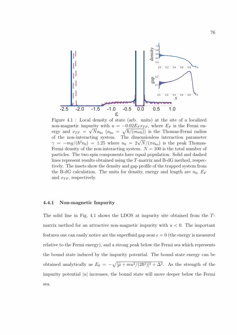
76

-2.5 -2.0 -1.5 -1.0 -0.5 0.0 0.5 1.0

ε

0.0 0.2 0.4 0.6 0.8 1.0

0.2

0.4

0.6

0.8

1.0

0.2 0.4 0.6 0.8 1.0

0.1

0.2

0.0

x

den

sity

gap

Figure 4.1 : Local density of state (arb. units) at the site of a localizednon-magnetic impurity with u = −0.02EFxTF , where EF is the Fermi en-ergy and xTF =

√Naho (aho =

√~/(mω0)) is the Thomas-Fermi radius

of the non-interacting system. The dimensionless interaction parameterγ = −mg/(~2n0) = 1.25 where n0 = 2

√N/(πaho) is the peak Thomas-

Fermi density of the non-interacting system. N = 100 is the total number ofparticles. The two spin components have equal population. Solid and dashedlines represent results obtained using the T -matrix and B-dG method, respec-tively. The insets show the density and gap profile of the trapped system fromthe B-dG calculation. The units for density, energy and length are n0, EFand xTF , respectively.

4.4.1 Non-magnetic Impurity

The solid line in Fig. 4.1 shows the LDOS at impurity site obtained from the T -

matrix method for an attractive non-magnetic impurity with u < 0. The important

features one can easily notice are the superfluid gap near ϵ = 0 (the energy is measured

relative to the Fermi energy), and a strong peak below the Fermi sea which represents

the bound state induced by the impurity potential. The bound state energy can be

obtained analytically as E0 = −√

[µ+mu2/(2~2)]2 +∆2. As the strength of the

impurity potential |u| increases, the bound state will move deeper below the Fermi

sea.

77

To confirm that these results still hold when a trapping potential is present, as is

always the case in the experiment, we add a harmonic potential VT = mω20x

2/2 to the

system and perform the calculation using the Bogoliubov-de Gennes (B-dG) method.

The dashed line in Fig. 4.1 represents the LDOS at the non-magnetic impurity site

(x = 0) calculated using the B-dG method. The agreement with the T -matrix method

is satisfactory. The remaining discrepancies (in particular the position of the bound

state) can be understood as the T -matrix method neglects the trapping potential and

is not fully self-consistent: the values of the chemical potentials, densities and pairing

gap used in the T -matrix calculation are taken to be those from the B-dG result in

the absence of the impurity. The insets of Fig. 4.1 demonstrate the density and gap

profiles of the trapped system. The Friedel oscillation with a spatial frequency close

to 2kF , where kF is the Fermi wave number, can be easily identified near the impurity.

4.4.2 Magnetic Impurity

The solid lines in Fig. 4.2(a),(b) display the LDOS at the magnetic impurity site

for the two spin species obtained using the T -matrix method. Here the impurity

potential is attractive (repulsive) for spin-up (down) atoms which creates a resonant

state below the Fermi sea for spin up atoms manifested by the peak near ϵ = −2EF

in Fig. 4.2(a). As the strength of the impurity potential |u| increases, the resonant

state will move deeper below the Fermi sea. Besides this resonant state, both ρ↑(ϵ)

and ρ↓(ϵ) exhibit an additional peak near ϵ = 0, which signals the presence of a mid-

gap bound state [127, 128, 129]. In the limit of weak interaction, the position of the

mid-gap bound state is given by the T -matrix method as:

E0 = ±∆1− (uπρ0/2)

2

1 + (uπρ0/2)2, (4.88)

78

ε x

den

sity

gap

( c)

(d)

(a)

(b)

-2.0 -1.0 0.0 1.0

0.0 0.2 0.4 0.6 0.8 1.0

0.2

0.4

0.6

0.8

1.0

0.1

0.2

-2.0 -1.0 0.0 1.0

0.0 0.2 0.4 0.6 0.8 1.0

n↑

n↓

0.04 0.12

0.4

0.8

x

Figure 4.2 : (a) Density of states for spin up atoms. (b) Density of statesfor spin down atoms. (c) Density profiles for both spin species. (d) Gapprofile. In (a) and (b) solid and dashed lines represent results obtainedusing the T -matrix and B-dG method, respectively. The dashed curve in(d) is the gap profile without the impurity. For all plots, N↑ = N↓ = 50,and u = −0.02EFxTF , where EF is the Fermi energy and xTF =

√Naho

is the Thomas-Fermi radius of the non-interacting system. The harmonicoscillator length and Thomas Fermi density at the origin are defined by aho =√

~/(mω0) and n0 = 2√N/(πaho). The dimensionless interaction parameter

γ = −mg/(~2n0) = 1.25. The units for density, energy and length are n0,EF and xTF , respectively.

where ρ0 is the density of states at the Fermi sea, and the + (−) sign refers to the spin-

up (-down) component. The mid-gap bound state is thus located outside the band

and inside the pairing gap. As the strength of the impurity |u| increases, the mid-gap

moves from the upper gap edge to the lower gap edge for the spin-up component and

moves oppositely for the spin-down component.

The dashed line in Fig. 4.2(a),(b) represents the LDOS at the magnetic impurity

site (x = 0) calculated using the B-dG method. The agreement with the T -matrix

method is satisfactory. The density and gap profiles of the trapped system are illus-

trated in Fig. 4.2(c),(d). Friedel oscillations with a spatial frequency close to 2kF can

79

be seen in the density profiles near the impurity. The magnetic impurity tends to

break Cooper pairs, leading to a reduced gap size near the impurity as can be seen

from Fig. 4.2(d).

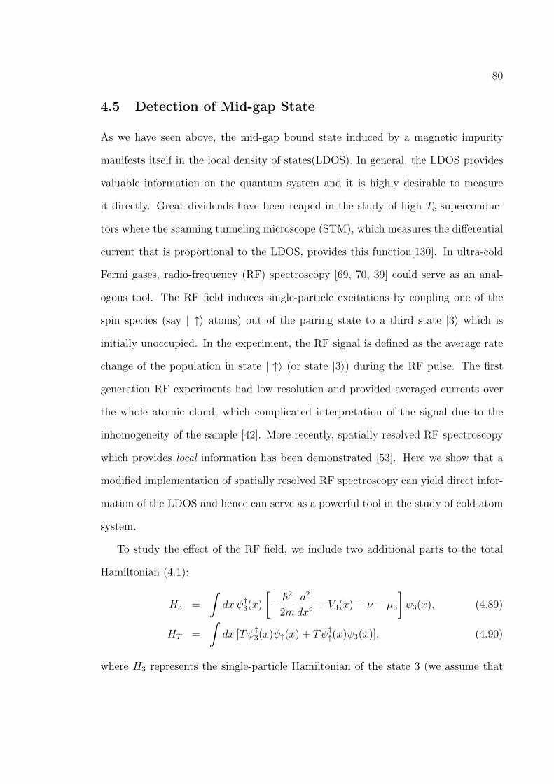
80

4.5 Detection of Mid-gap State

As we have seen above, the mid-gap bound state induced by a magnetic impurity

manifests itself in the local density of states(LDOS). In general, the LDOS provides

valuable information on the quantum system and it is highly desirable to measure

it directly. Great dividends have been reaped in the study of high Tc superconduc-

tors where the scanning tunneling microscope (STM), which measures the differential

current that is proportional to the LDOS, provides this function[130]. In ultra-cold

Fermi gases, radio-frequency (RF) spectroscopy [69, 70, 39] could serve as an anal-

ogous tool. The RF field induces single-particle excitations by coupling one of the

spin species (say | ↑⟩ atoms) out of the pairing state to a third state |3⟩ which is

initially unoccupied. In the experiment, the RF signal is defined as the average rate

change of the population in state | ↑⟩ (or state |3⟩) during the RF pulse. The first

generation RF experiments had low resolution and provided averaged currents over

the whole atomic cloud, which complicated interpretation of the signal due to the

inhomogeneity of the sample [42]. More recently, spatially resolved RF spectroscopy

which provides local information has been demonstrated [53]. Here we show that a

modified implementation of spatially resolved RF spectroscopy can yield direct infor-

mation of the LDOS and hence can serve as a powerful tool in the study of cold atom

system.

To study the effect of the RF field, we include two additional parts to the total

Hamiltonian (4.1):

H3 =

∫dxψ†

3(x)

[− ~2

2m

d2

dx2+ V3(x)− ν − µ3

]ψ3(x), (4.89)

HT =

∫dx [Tψ†

3(x)ψ↑(x) + Tψ†↑(x)ψ3(x)], (4.90)

where H3 represents the single-particle Hamiltonian of the state 3 (we assume that

81

atoms in state 3 do not interact with other atoms, so there is no final state effect), with

V3 being the trapping potential of the state and ν the detuning of the RF field from

the atomic transition, HT represents the coupling between state 3 and spin-up atoms.

Since the RF photon wavelength is much larger than the typical size of the atomic

cloud, the coupling strength T can be regarded as a spatially invariant constant. For

weak RF coupling, one may use the linear response theory [64, 65, 131, 132, 133]

to obtain the RF signal which is proportional to I(x) = ddt⟨ψ†

3(x)ψ3(x)⟩. Under the

linear response theory, we have

I(x) ∝∫dx′dωA↑(x, x

′;ω)A3(x′, x, ω + µ↑ − µ3)f(ω) (4.91)

where f(ω) is the Fermi distribution function which reduces to the step function at

zero temperature, Aα is the spectral function for state α. As state 3 is non-interacting,

we have A3 =∑

nϕn(x)ϕ∗n(x

′)δ(ω + µ↑ + ν − ϵn), where ϕn is the single-particle

eigenfunction of state 3 and ϵn is the eigen-energy, respectively. The key step in our

proposal is that in the case where V3 represents an optical lattice potential in the

tight-binding limit, the dispersion of state 3 is proportional to the hopping constant

t which decreases exponentially as the lattice strength is increased. In this way the

optical lattice changes the effective mass of state 3. For sufficiently large lattice

strength, we may therefore neglect the dispersion of state 3 since the lowest band is

nearly flat. In other words, under such conditions, ϵn = ϵ becomes an n-independent

constant. Consequently A3(x, x′) ∼ δ(x − x′) where the information of state 3 is

washed out. In this limit and at zero temperature, the RF signal is then directly

related to the LDOS of state | ↑⟩ as:

I(x) ∝ ρ↑(x,−µ↑ − ν + ϵ)Θ(µ↑ + ν − ϵ) . (4.92)

and the spatially resolved RF spectroscopy becomes a direct analog of the STM. A

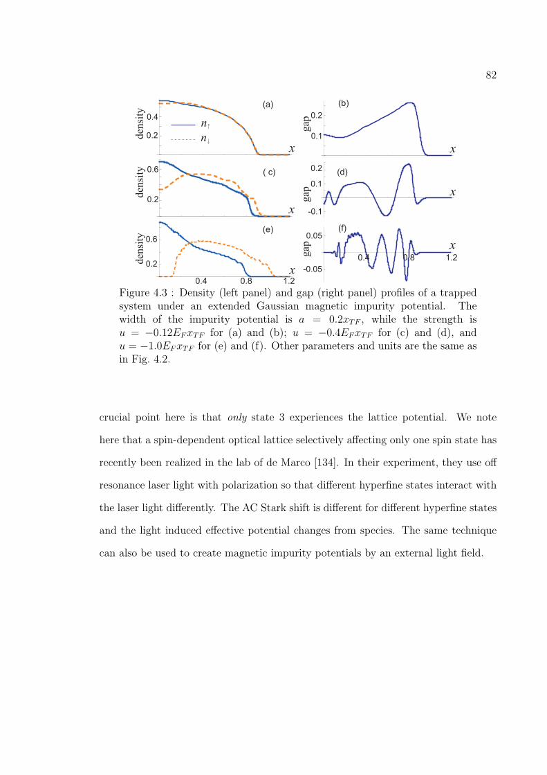
82

(a) (b)

( c) (d)

n↑

n↓

x

0.4 0.8 1.2

-0.05

0.05

0.4 0.8 1.2

0.2

0.6

den

sity

gap x

0.2

0.6

den

sity

gap

-0.1

0.1

0.2

0.2

0.4

den

sity

0.1

0.2

gap

x

x x

x

(e) (f)

Figure 4.3 : Density (left panel) and gap (right panel) profiles of a trappedsystem under an extended Gaussian magnetic impurity potential. Thewidth of the impurity potential is a = 0.2xTF , while the strength isu = −0.12EFxTF for (a) and (b); u = −0.4EFxTF for (c) and (d), andu = −1.0EFxTF for (e) and (f). Other parameters and units are the same asin Fig. 4.2.

crucial point here is that only state 3 experiences the lattice potential. We note

here that a spin-dependent optical lattice selectively affecting only one spin state has

recently been realized in the lab of de Marco [134]. In their experiment, they use off

resonance laser light with polarization so that different hyperfine states interact with

the laser light differently. The AC Stark shift is different for different hyperfine states

and the light induced effective potential changes from species. The same technique

can also be used to create magnetic impurity potentials by an external light field.

83

4.6 Extended Impurity

Now we turn to the extended impurity. We use Gaussian impurity potentials with

finite width Uσ(x) = uσe−x2/a2/(a

√π). Since we obtain all of the previous (delta

function) physics for narrow widths, we focus on relatively wide potentials. Examples

of the density and gap profiles obtained from our B-dG calculations are shown in

Fig. 4.3. For an extended impurity potential of sufficient width, the Friedel oscillations

are suppressed. This is because now the impurity is complicated and has structure.

Friedel oscillations interfere with each other and become smooth.

Under appropriate conditions, the gap profiles exhibit FFLO-like oscillations [135,

136], which has recently received considerable attention in studies of ultra-cold atoms

[137, 138, 139, 140, 141]. In the FFLO state, due to population imbalance, the Fermi

surfaces of two species mismatch. This causes the phase of the Cooper pair to have a

periodic pattern in real space with a characteristic wavelength signifying the center-of-

mass momentum of the pair. In previous experiments, polarized Fermi gas have been

realized by preparing the gas with an overall population imbalance. Here the overall

population is balanced but the magnetic impurity breaks the local population balance

and by tailoring the strength and/or the width of the magnetic impurity, one is able

to control the magnitude of the population imbalance as shown in Fig. 4.3 which

in turn controls the nature of the induced FFLO state. In Fig. 4.3, by changing

the magnetic impurity strength, the system evolves from a balanced system to an

imbalanced system and the pairing changes from BCS pairing to FFLO pairing. The

impurity therefore provides us with a controlled way to create FFLO state.

For simplicity, we have thus far focused on 1D systems. However, we have verified

that the essential physics is also valid in higher dimensions. As an example, we

illustrate in Fig. 4.4 the effect of an extended magnetic impurity in a 3D trapped

84

den

sity

gap

n↑

n↓

x/xTF

x/xTF

Figure 4.4 : Density (upper panel, in units of (2EF )3/2/(6π2)) and gap (lower

panel, in units of EF ) profiles along the x-axis of a 3D trapped system underan extended magnetic impurity potential. The impurity potential is uniformalong the radial direction and has a Gaussian form with width a = 0.3xTFalong the x-axis. The strength of the impurity is u = −0.07EFxTF . Theatom-atom interaction is characterized by the 3D scattering length as. Herewe have used 1/(kFas) = −0.69.

system obtained by solving the B-dG equations [125, 126]. Here a total of 1100 atoms

are trapped in an elongated cylindrical trapping potential V (r, x) = m2(ω2

⊥r2 + ω2

xx2)

with trap aspect ratio ω⊥/ωx = 50. The magnetic impurity centered at the origin, is

radially uniform and has a Gaussian profile along the axial direction (x-axis). From

the density and gap profiles shown in Fig. 4.4, one can easily identify the induced

FFLO regions both near the center and the edge of the trap. In particular, the density

oscillations in the spin-down component near trap center may be used as a signature

of the FFLO state.

85

Chapter 5

Summary and Conclusions

In conclusion, the BEC-BCS crossover theory is becoming one of the most exciting

fields in cold atoms and condensed matter physics. It connects to many other fields

of physics, such as cuprate high temperature superconductivity, excitons in semi-

conductors, neutron stars in astronomy, and the vacuum condensate for the early

universe. It is also a candidate for quantum computation and quantum information.

In addition, there are still many open questions. One is the accuracy for perturba-

tion theory to give the quantitative explanations for the crossover experiment. In the

crossover regime, fermions are strongly correlated and there is no small parameter to

do the perturbative expansion. New progress occurs using new approaches, for exam-

ple, large N expansion[142], [143] and ϵ dimensionality[144]. Another exciting field

is the population imbalanced system, where the pairing mechanism for population

imbalanced fermions raises long standing interest.

For Fermi superfluids, how to detect pairing is one of the biggest problems. We

proposed to use optical spectroscopy in an EIT setting to probe the fermionic pairing

in Fermi gases in Chapter 2. We have demonstrated that the EIT technique offers

an extremely efficient probing method and is capable of detecting the onset of pair

formation (i.e., determining T ∗) due to its spectral sensitivity. With a sufficiently

weak probe field, the whole spectrum may be obtained in a nearly non-destructive

fashion via a relatively fast scan of probe frequency, without the need of repeatedly

re-preparing the sample. We noted that in this work, we have focused on probing

86

the atomic system using photons. In the future, it will also be interesting to study

how we can use atomic Fermi gas to manipulate the light. Superfluid fermions can

serve as a new type of nonlinear media for photons. Also, we want to remark that,

in this work, as a proof-of-principle, we have only considered a homogeneous system.

As usual, the trap inhomogeneity can be easily accounted for within the local density

approximation. Nevertheless, we noted that the capability of detecting the onset of

pairing remains the same even in the presence of the trap. Furthermore, as optical

fields are used in this scheme, one may focus the probe laser beam such that only

a small localized portion of the atomic cloud is probed, hence there is no need to

average over the whole cloud.

One exciting field in both cold atom and condensed matter physics is the topo-

logical phase. Spin-orbit coupling is one of the ways to introduce this novel property.

In chapter 3, we provide a detailed theoretical description of a two-component Fermi

gas with Rashba spin-orbit coupling and external Zeeman field, under the framework

of the functional path integral formalism. Many important and experimentally rele-

vant physical quantities in both two- and many-body situations — such as the bound

state energy, the effective mass of the two-body bound state, the chemical potential,

gap parameter, pairing correlation, quasi-particle dispersion, density of states, spin

structure factor, etc. — are calculated in a rather straightforward way using this

method. The spin-orbit coupling in general favors the formation of Cooper pair and

bound state. In particular, we have found that when a Rashba ring exists for the

single-particle ground state, a two-body bound state exists regardless of the sign of

the s-wave scattering length.

For the sake of simplicity, we have only presented the zero-temperature results in

this paper. The formalism and the relevant equations we have derived are nevertheless

87

valid for finite temperatures. In addition, we have focused on a uniform system. To

take the trap into account, one may adopt the local density approximation [92, 96],

under which the trapped Fermi gas was treated as the sum of many small cells with

a local chemical potential µ(r) = µ − Vtrap(r). In one of our works [92], we have

shown that the important qualitative features of the system, like the mixed-spin

pairing, anisotropy, enhanced pairing field, etc., are not affected by the presence of

the trap. A self-consistent way to include the effects of the trapping potential is

to use the Bogoliubov-de Gennes (B-dG) formalism. For large number of atoms as

used in most experiments, we expected that the local density approximation should be

quite accurate. However, for a system with relatively small number of atoms and tight

trapping confinement, or in the case of a vortex state where the order parameter varies

significantly in a short length scale, the B-dG approach will be more appropriate.

One crucial feature of the system arising from the spin-orbit coupling is that the

superfluid transition temperature is greatly enhanced [93]. The mean-field calculation

which we have focused on in this work is not expected to provide an accurate estimate

of the transition temperature, particularly for systems with strong interaction. As

we have outlined in Sec. 3.2 of chapter 3, the Gaussian fluctuations on top of the

mean-field level can be accounted for using the functional path integral formalism.

This will lead to a much more accurate calculation of the transition temperature. We

plan to address this issue in a future work. Furthermore, the spin structure factor is

calculated in the static model which neglects collective excitation. We plan to add

this using a dynamic model, such as the random phase approximation(RPA).

In chapter 4, we have investigated the effects of a single classical impurity on a

neutral fermionic superfluid. We show that a single classical impurity can be used

to manipulate novel quantum states in a Fermi gas. For example, magnetic impu-

88

rity will induce a mid-gap bound state inside the pairing gap for both spin species.

We have proposed an STM-like scheme based on the modified spatially resolved RF

spectroscopy to measure the local density of states, from which the mid-gap bound

states can be unambiguously detected. As different quantum phases of cold atoms

will manifest themselves in their distinct LDOS, we expect this method will find im-

portant applications beyond what is proposed here and become an invaluable tool in

the study of quantum gases. Finally, by considering an extended magnetic impurity

potential in both 1D and 3D systems, we demonstrated the realization of the still

unobserved FFLO phase in a controlled manner.

Interesting future directions may involve the study of periodic or random arrays

of localized impurities which may be exploited to induce novel quantum states in

Fermi superfluids and the consideration of a quantum impurity with its own internal

degrees of freedom. Such a system may allow us to explore the Kondo physics in cold

atoms.

89

Bibliography

[1] M. H. Anderson, J. R. Ensher, M. R. Matthews, C. E. Wieman, and E. A.

Cornell, Science 269, 198 (1995).

[2] C. C. Bradley, C. A. Sackett, J. J. Tollett, and R. G. Hulet, Phys. Rev. Lett.

75, 1687 (1995).

[3] K. B. Davis, M.-O. Mewes, M. R. Andrews, N. J. van Druten, D. S. Durfee, D.

M. Kurn, and W. Ketterle, Phys. Rev. Lett. 75, 3969 (1995).

[4] B. DeMarco and D.S. Jin, Science 285 1703 (1999).

[5] L. N. Cooper, Phys. Rev. 104, 1189 (1956).

[6] J. Bardeen, L. N. Cooper, and J. R. Schrieffer, Phys. Rev. 108, 1175 (1957).

[7] J. Bardeen, L. N. Cooper, and J. R. Schrieffer, Phys. Rev. 106, 162 (1957).

[8] A. J. Leggett, Rev. Mod. Phys. 47, 331 (1975).

[9] U. Fano, Phys. Rev. 124, 1866 (1961).

[10] H. Feshbach, Ann. Phys. (N.Y.) 19, 287 (1962).

[11] K. M. OHara, S. L. Hemmer, M. E. Gehm, S. R. Granade, and J. E. Thomas,

Science 298, 2179 (2002).

90

[12] T. Bourdel, J. Cubizolles, L. Khaykovich, K. M. F. Magalhes, S. J. J. M. F.

Kokkelmans, G. V. Shlyapnikov, and C. Salomon, Phys. Rev. Lett. 91, 020402

(2003).

[13] A.J. Legget, in Modern Trends in the Theory of Condensed Matter (Springer-

Verlag, 1980).

[14] H. T. C. Stoof, M. Houbiers, C. A. Sackett, and R. G. Hulet, Phys. Rev. Lett.

76, 10 (1996).

[15] G. Bruun, Y. Castin, R. Dum, and K. Burnett, Eur. Phys. J. D 7, 433 (1999).

[16] M. Holland, et al., Phys. Rev. Lett. 87, 120406 (2001).

[17] K. Huang, and C. N. Yang, Phys. Rev. 105, 767 (1957).

[18] L. D. Landau, and E. M. Lifshitz, Quantum Mechanics, 3rd ed. (Pergamon,

Oxford, 1987).

[19] T. L. Ho, Phys. Rev. Lett. 92, 090402 (2004).

[20] I. Bloch, J. Dalibard, and W. Zwerger, Rev. Mod. Phys. 80, 885 (2008).

[21] S. Giorgini, L. P. Pitaevskii, and S. Stringari, Rev. Mod. Phys. 80, 1215 (2008).

[22] W. Ketterle and M. W. Zwierlein, Making, probing and understanding ultracold

Fermi Gases, Proceedings of the International School of Physics Enrico Fermi,

Course CLXIV edited by M. Inguscio, W. Ketterle, and C. Salomon, (IOS Press,

Amsterdam, 2007), p.95.

[23] R. B. Diener, R. Sensarma, and M. Randeria, Phys. Rev. A 77, 023626 (2008).

91

[24] D.S. Petrov, et al., Phys. Rev. Lett. 93 090404 (2004).

[25] G.E. Astrakharchik, et al., Phys. Rev. Lett. 93 200404 (2004).

[26] D.J. Thouless, Ann. Phys. 10, 553 (1960).

[27] M. Gell-Mann and K.A. Brueckner, Phys. Rev. 106, 364 (1958).

[28] E.W. Montroll and J.C. Ward, Phys. Fluids 1, 55 (1958).

[29] P. Nozieres and S. Schmitt-Rink, J. Low Temp. Phys. 59, 195 (1985).

[30] Y. Ohashi and A. Griffin, Phys. Rev. Lett. 89 130402 (2002).

[31] A. Perali, P. Pieri, L. Pisani, and G. C. Strinati, Phys. Rev. Lett. 92, 220404

(2004).

[32] H. Hu, X.-J. Liu, and P. Drummond, Europhys. Lett. 74, 574 (2006).

[33] R. Haussmann, Phys. Rev. A 75 023610 (2007).

[34] J. Stajic, et al., Phys. Rev. A 69 063610 (2004).

[35] Q.J. Chen, et al., Phys. Rept. 412 1 (2005).

[36] M. Greiner, et al., Nature 426 537 (2003).

[37] C.A. Regal, et al., Phys. Rev. Lett. 92 040403 (2004).

[38] M.W. Zwierlein, et al., Phys. Rev. Lett. 92 120403 (2004).

[39] C. Chin, et al., Science 305 1128 (2004).

[40] M.W. Zwierlein, et al., Nature 435 1047 (2005).

92

[41] J. Kinnunen, et al., Science 305 1131 (2004).

[42] P. Massignan, G. M. Bruun, and H. T. C. Stoof, Phys. Rev. A 77 031601(R)

(2008).

[43] Y. Ohashi and A. Griffin, Phys. Rev. A 72, 013601 (2005).

[44] Z. Yu and G. Baym, Phys. Rev. A 73, 063601 (2006).

[45] G. Baym, C. J. Pethick, Z. Yu and M. W. Zwierlein, Phys. Rev. Lett. 99, 190407

(2007).

[46] A. Perali, P. Pieri, and G. C. Strinati, Phys. Rev. Lett. 100, 010402 (2008).

[47] S. Basu and E. Mueller, Phys. Rev. Lett. 101, 060405 (2008).

[48] Y. He, C.-C. Chien, Q. J. Chen, and K. Levin, Phys. Rev. Lett 102, 020402

(2009).

[49] A. Schirotzek, Y. Shin, C.H. Schunck, and W. Ketterle, Phys. Rev. Lett. 101 ,

140403 (2008).

[50] C.H. Schunck, Y. Shin, A. Schirotzek, and W. Ketterle, Nature 454 , 739 (2008).

[51] J. T. Stewart, J. P. Gaebler, and D. S. Jin, Nature (London) 454, 744 (2008).

[52] J. P. Gaebler, J. T. Stewart, T. E. Drake, D. S. Jin, A. Perali, P. Pieri, and G.

C. Strinati, Nature Phys. 6, 569 (2010).

[53] Y. Shin et al., Phys. Rev. Lett 99 090403 (2007).

[54] W. Zhang, C. A. Sackett, and R. G. Hulet, Phys. Rev. A 60, 504 (1999).

[55] F. Weig and W. Zwerger, Europhys. Lett. 49, 282 (2000).

93

[56] E. Altman, E. Demler, and M. D. Lukin, Phys. Rev. A 70, 013603 (2004).

[57] J. Ruostekoski, Phys. Rev. A 61, 033605 (2000).

[58] A. Minguzzi, G. Ferrari, and Y. Castin, Eur. Phys. J. D 17 49, 2001.

[59] C. P. Search, H. Pu, W. Zhang and P. Meystre, Phys. Rev. Lett. 88, 110401

(2002).

[60] R. Combescot, S. Giorgini, and S. Stringari, Europhys. Lett. 75 695 (2006).

[61] G. Veeravalli, E. Kuhnle, P. Dyke, and C. J. Vale, Phys. Rev. Lett. 101, 250403

(2008).

[62] E. D. Kuhnle, H. Hu, X.-J. Liu, P. Dyke, M. Mark, P. D. Drummond, P. Han-

naford, and C. J. Vale, Phys. Rev. Lett. 105, 070402 (2010).

[63] E. D. Kuhnle, S. Hoinka, P. Dyke, H. Hu, P. Hannaford, and C. J. Vale, Phys.

Rev. Lett. 106, 170402 (2011).

[64] P. Torma and P. Zoller, Phys. Rev. Lett. 85, 487 (2000).

[65] G. M. Bruun et al., Phys. Rev. A 64, 033609 (2001).

[66] G. M. Bruun and G. Baym, Phys. Rev. Lett. 93, 150403 (2004).

[67] J. Ruostekoski, Phys. Rev. A 60, R1775 (1999).

[68] I. Carusotto, and Y. Castin, Phys. Rev. Lett. 94, 223202 (2005).

[69] C.A. Regal and D.S. Jin, Phys. Rev. Lett. 90, 230404 (2003).

94

[70] S. Gupta, Z. Hadzibabic, M. W. Zwierlein, C. A. Stan, K. Dieckmann, C. H.

Schunck, E. G. M. van Kempen, B. J. Verhaar, and W. Ketterle, Science 300,

1723 (2003).

[71] K. -J. Boller, A. Imamoglu, and S. E. Harris, Phys. Rev. Lett. 66, 2593 (1991).

[72] M. Xiao, Y. Li, S. Jin, and J. Gea-Banacloche, Phys. Rev. Lett. 74, 666 (1995).

[73] E. Arimondo, in Progress in Optics XXXV, ed. E. Wolf (Elsevier, Amsterdam,

1996), p. 257.

[74] L. V. Hau, S. E. Harris, Z. Dutton, C. H. Behroozi, Nature 397, 594-598 (1999).

[75] M. M. Kash, V. A. Sautenkov, A. S. Zibrov, L. Hollberg, G. R. Welch, M. D.

Lukin, Y. Rostovtsev, E. S. Fry, and M. O. Scully, Phys. Rev. Lett. 82, 5229-

5232(1999).

[76] R.W. Boyd and D. J. Gauthier, in Progress in Optics, ed. E. Wolf (Elsevier,

Amsterdam, 2002), Vol 43, p. 497.

[77] M. Fleischhauer and M. D. Lukin, Phys. Rev. Lett. 84, 5094 (2000).

[78] C. Liu, Z. Dutton, C. Behroozi, and L. V. Hau, Nature 409. 490 (2001).

[79] K. J. Weatherill, J. D. Pritchard, R. P. Abel, M. G. Bason, A. K. Mohapatra

and C. S. Adams, J. Phys. B: At. Mol. Opt. Phys. 41 201002 (2008).

[80] M. W. Zwierlein, A. Schirotzek, C. H. Schunck, and W. Ketterle, Science 311,

492 (2006).

[81] G. B. Partridge, W. Li, R. I. Kamar, Y. Liao, and R. G. Hulet, Science 311, 503

(2006).

95

[82] H. Y. Ling, Y.-Q. Li, and M. Xiao, Phys. Rev. A 53, 1014 (1996).

[83] See, for example, G. D. Mahan, Many-Particle Physics (Indiana Univ., 1980).

[84] Y.-J. Lin, R. L. Compton, A. R. Perry, W. D. Phillips, J. V. Porto, and I. B.

Spielman, Phys. Rev. Lett. 102, 130401 (2009).

[85] Y.-J. Lin, R. L. Compton, K. Jimenez-Garcıa, J. V. Porto, and I. B. Spielman,

Nature (London) 462, 628 (2009).

[86] Y-J. Lin, R. L. Compton, K. Jimenez-Garcıa, W. D. Phillips, J. V. Porto, and

I. B. Spielman, Nature Phys. 7, 531 (2011).

[87] Y.-J. Lin, K. Jimenez-Garcıa, and I. B. Spielman, Nature (London) 471, 83

(2011).

[88] Z. Fu, P. Wang, S. Chai, L. Huang, and J. Zhang, e-print arXiv:1106.0199.

[89] For a brief review, see, for example, Jean Dalibard, Fabrice Gerbier, Gediminas

Juzeliu-nas, Patrik Ohberg, eprint arXiv:1008.5378.

[90] J. P. Vyasanakere, and V. B. Shenoy, Phys. Rev. B 83, 094515 (2011).

[91] J. P. Vyasanakere, S. Zhang, and V. B. Shenoy,Phys. Rev. B 84, 014512 (2011).

[92] H. Hu, L. Jiang, X.-J. Liu, and H. Pu, e-print arXiv:1105.2488.

[93] Z.-Q. Yu, and H. Zhai, e-print arXiv:1105.2250.

[94] C. Zhang, S. Tewari, R.M. Lutchyn, and S. Das Sarma, Phys. Rev. Lett. 101,

160401 (2008).

[95] M. Gong, S. Tewari, and C. Zhang, e-print arXiv:1105.1796.

96

[96] W. Yi, and G.-C. Guo, e-print arXiv:1106.5667.

[97] J.D. Sau, R. Sensarma, S. Powell, I. B. Spielman, and S. Das Sarma, Phys. Rev.

B 83, 140510(R) (2011)

[98] M. Iskin, and A. L. Subaas, Phys. Rev. Lett. 107, 050402 (2011).

[99] M. Iskin, and A. L. Subaas, e-print arXiv:1108.4263.

[100] T. Ozawa, and G. Baym, e-print arXiv:1107.3162.

[101] L. Han, and C. A. R. Sa de Melo, e-print arXiv:1106.3613.

[102] K. Seo, L. Han, and C. A. R. Sa de Melo, e-print arXiv:1108.4068.

[103] L.P. Gor’kov, and E.I. Rashba, Phys. Rev. Lett. 87, 037004 (2001).

[104] S. Tewari, T.D. Stanescu, J.D. Sau, and S. Das Sarma, New J. Phys. 13, 065004

(2011).

[105] M. Sato, Y. Takahashi, and S. Fujimoto, Phys. Rev. Lett. 103, 020401 (2009);

Phys. Rev. B 82, 134521 (2010).

[106] C. A. R. Sa de Melo, M. Randeria, and J. R. Engelbrecht, Phys. Rev. Lett. 71,

3202 (1993).

[107] M. Randeria, in Bose-Einstein Condensation, edited by A. Griffin, D. W. Snoke,

and S. Stringari, (Cambridge University Press, Cambridge, England, 1995), p.

355-392.

[108] X.-J. Liu and H. Hu, Europhys. Lett. 75, 364 (2006).

97

[109] L. Jiang, L. O. Baksmaty, H. Hu, Y. Chen, and H. Pu, Phys. Rev. A 83,

061604(R) (2011).

[110] A. V. Balatsky, I. Vekhter, and J.-X. Zhu, Rev. Mod. Phys. 78, 373 (2006).

[111] H. Alloul et al., Rev. Mod. Phys. 81, 45 (2009).

[112] A.P. Mackenzie et al., Phys. Rev. Lett. 80, 161 (1998).

[113] P. T. Sprunger et al., Science 275, 1764 (1997).

[114] A. J. Millis, Solid State Commun. 126, 3 (2003).

[115] G. Modugno, Rep. Prog. Phys. 73, 102401 (2010).

[116] C. Zipkes et al., Nature 464, 388 (2010).

[117] K. Targonska and K. Sacha, Phys. Rev. A 82, 033601 (2010)

[118] E. Vernier et al., Phys. Rev. A 83, 033619 (2011).

[119] I. Bausmerth et al., Phys. Rev. A 79, 043622 (2009).

[120] P. J. Hirschfeld, D. Vollhard, and P. Wolfle, Solid State Commun. 59, 111

(1986).

[121] R. Joynt, J. Low Temp. Phys. 109, 811 (1997).

[122] P. de Gennes, Superconductivity of Metals and Alloys (Addison-Wesley, New

York, 1966).

[123] X.-J. Liu, H. Hu, and P. D. Drummond, Phys. Rev. A 75, 023614 (2007).

[124] X.-J. Liu, H. Hu, and P. D. Drummond, Phys. Rev. A 76, 043605 (2007).

98

[125] L. O. Baksmaty et al.,Phys. Rev. A 83, 023604 (2011).

[126] L. O. Baksmaty, H. Lu, C. J. Bolech, and H. Pu, New J. Phys. 13, 055014

(2011).

[127] L. Yu, Acta Phys. Sin. 21, 75 (1965).

[128] H. Shiba, Prog. Theor. Phys. 40, 435 (1968).

[129] A. I. Rusinov, Sov. Phys. JETP 29, 1101 (1969).

[130] Ø. Fischer et al., Rev. Mod. Phys. 79, 353 (2007).

[131] J. Kinnunen, M. Rodriguez, and P. Torma, Phys. Rev. Lett. 92, 230403 (2004).

[132] Y. He, Q. Chen, and K. Levin, Phys. Rev. A 72, 011602(R) (2005).

[133] Y. He et al., Phys. Rev. A 77, 011602(R) (2008).

[134] D. McKay and B. DeMarco, New J. Phys. 12 055013 (2010).

[135] P. Fulde and R. A. Ferrell, Phys. Rev. 135 A550 (1964).

[136] A. I. Larkin and Y. N. Ovchinnikov Sov. Phys.-JETP 20 762 (1965).

[137] Y.-A. Liao et al., Nature 467, 567 (2010).

[138] G. Orso, Phys. Rev. Lett. 98, 070402 (2007).

[139] H. Hu, X.-J. Liu, and P. D. Drummond, Phys. Rev. Lett. 98, 070403 (2007).

[140] I. Zapata et al., Phys. Rev. Lett. 105, 095301 (2010).

[141] K. Sun et al., Phys. Rev. A 83, 033608 (2011).

99

[142] P. Nikolic and S. Sachdev, Phys. Rev. A 75 033608 (2007).

[143] M.Y. Veillette, et al., Phys. Rev. A 75 043614 (2007).

[144] Y. Nishida and D.Y. Son, Phys. Rev. Lett. 97 050403 (2006).