HYDROMETEORO:tOGICAL REPO~T NO. 48

Probable M~um Precipitation _and Snowmelt Criteria For Red River

of the North Above Peinhina, and Souris River Above·Minot~

-North Dakota

U.S.-DEPARTMENT OF CO:t\IMEJtCE NATION~ OCEANIC AND ATMOSPHERiC ADMINISTRATION-

U.S. DEPARTMENT OF THE ARMY CORPS OF ENGINEERS

Waobington, D.C. May 1973

*No *.:.No *No *No *No *No *No

• -HYDROMETEOROLOGICAL REPORTS ' ..

I I ,MaXImum possible p~eCipitatmn Over' the Ompompan;,o~uc B~ aboVe ti.!llon,Village;, Vt 1~43 2 Ma.xtmuip. possible p_rectpl'~_ation Over the' Ohm River Basm abo~e Pittsburgh, ~Pa 1942 3 MaxU:num possible preCxpit&tu)n over the' Sacramento ,Basm of-Cahforma 1943' 4 MaXllllum poSsible precipitatiOn over the Panama. C~al Basm _, 1943 ~ 5' Thunderstorm ramfai! '194'7' • ' ' · · '6 A-prehm.IDary report on f.he Probable o.ccurreD.ce of excessive Precipitatton over, Fort SupplY, BB.sm, OklO: ~9-38. 7 Worst probable meteoro~oglcal conchtmh on Mtll C:r:~~ek, Butler and Hamilton ~ounties, OhiO ~1937 <VnplJb-

hshed) Supplement, 1938-- - . · ' _ " ·-*No 8 A hydrometeorologtcal aiialySis of posstble maXJmum pl'eCtpitatlon over St FranciS Riv'er .Basm'·abo've'•Wappa-.

pello, Mo 1938 · ' - ... 1 , ._, ,_ _. ~ .< , , ,

, *No' 9. A r~port· on tbe,possible·Oc_currence 9f~piaXllll~J'Precipitation over·Wmte River Basin. abo~e ~ud->M~nmtam _ Dam site, Wash 1939 '· ~ , ~~- -, ~ _; ' ' . :r ,. _ z' ~ ,, ,_ .._.

'i!No 10 M&Xllllum possible ratDfall over the/Arkansas River Bk.sul above Caddoa, ,Cold' 1939 Supplement, 1939 *No u- A prehmm'ary report on the ma.xunum·possible precipitation-oVer the Dorena, Cottage• GroVe, and Fern Rtdge

~ Basms m the Willamette Basm, Oreg. 1939 .. _,o ; ' ) '- _ _,. ' _-. , -... - • - •

'*No *No *No

J ' - ~ ~ ' ' ' " 12 MB.XImum posstble precipitation over the Red River- Basm above Demson,.Tex 1939. 13 A report oil the maXImum p6'Srnble pr,ectpiiation over Cherry Cx:~ek Basiil:mL ColorB.dO_.';l940 ' 14 The frequency of fiood"producmg ramfall over the PaJaro -River Basm nl Cah.(om1a 1940

*No 15. A report On depth-frequency relations ·of thunde'rstorm railuaU·on the Sevier Basin, .Utah. 1941 *No 16. A prehn:imar,y report· ~n the maxnnum 'p_ossible preCipitation--Over the PrOto~ag aD:~-Rappa'hailnoc~ Rlver

BB.SJns 1943 - ' -, , , .-.. ·" *No 17 MaXliD.um possible,pre~Ipit8.tJ.on over'th; PeCos Ba.sm of Ne~Meh~o 19~ ._(Unpublished.) ¥_.- ~ '

*No 18. TeD.tat~ve estimates of maXllll\iin· possible flood-producmg ineteorologtcal conditions m the ColUmbia RIVer • Basm 1945 - . - • · .

*No 19. PrehmmarY report oD. depth-duratiOn-frequency char&cterist~~ of precipita~IOn ~ver the Muskmgum' Basm for 1- to 9-we~k periods 1945 -;- ~ - '~ , ·- l

*No 20 An estimate Of iiiaxn::D.um possible fiood-Pioducmg meteorological comhtwDs m the M1ssoun River Basm above Garns·on Dam Site 1945. , ' ~ r - - - ~ :-.

*No- 21_ A hydrometeo.rofogtcafstud_y of tBe Lo~ ~gef~_area· 1939. , , - ~, ~-- .. *No 21A Prehmmary reportron',m&XImum,possible prempit·ation, Los Angeles area, Cahforma.-1944 *No 21B ReVIsed report On maxnn.Wh lmssible precipltatton, Los Angeles--area, Cahforn~ "19-45

' ' I - • ~

'i!N o 22 An estunate of.IpaXImum possible_ flood-producmg meteorological conditions )D. the MISsouri Riyer Basm between - Garrison and Fort Randall'" 1946 - _ ,. ~ ~ ' - _

*No 23 Generalized estimates of maxunUm possible precipitation oVer the Uruted Si&..tes east of the 105th mendian, for areas of 10,200; 8.nd 500 sql.!are mJ.les 1947 - -; _ ·

*No 24 M8.X1Illum posstble preCipitation over~the San Joaqwn Basm, Cahf 1947: _ - -*No 25 RepreseD.tative 12--hour dewpoints m maJor United States storms east of the Qontmental Divide" 1947. *No 25A Representative 12-hour'dewpomts'm DiaJor United States storms east,of the Contmental DIVIde 2d editiOn'.

1949 *No. *No *No

.*No

26 An11lysiS or wmds over :[.ake Okeechobee durmg tropical storm of August 26-27, 1949 1951 , -, 27. Estunate of maxnnum po·ss1ble px:emp1tation, Rio Grande Basm, Foi't Qwtman to Zapata. 1951 28 'GenCrahZed estimate of maXImum possible-precipitation over New-England and New YOrk 1952. 29 Season~l variation of the standard proJeCt storm for areas of 2oo and 1,000 square mlles east of '105th meridian

1953. . ' --*No. 30 •No 31 *No 32

Meteorology of floods at St LoUIS' 1953 (Unpubhshed) AnalysiS and synthesiS of hurncane wmd patterns over Lake Qkeechobee, Florid&, 1954 Charactenstics of Umted States hurricanes pertment to levee des~gn for Lake $)keechobee, Florida 1954 Seasonal van8.t1on of the probable maXImum1Pfecipita.tiOn east of the 105th meru:han for areas from 10 to 1,000 No. 33

No No.

sqUare Dllles and durations of 6, 12, 24, and 48 hours 1956 ' 34 Meteorology of flo0d-prodticmg'storms m the Missis'stppi River BH.sm: 1956. 35' Meteorolog,y of hypothetiCal flood' sequences m the MlBSI~Sippi RIVe~-Basm 1959. ,,

• No 36 Interun report--probable maxnnum precipitation m· Cahforn1a 1961. Also available IS a supplement,. dated Octob_er.1969. , ' ·

' No No No. No No No No No No

37 Meteorology of hydrologically critical storms m Cahfol'D.la. 1962 38 Meteorology of flood-prod~"ing sto!ms m the Ohio River Ba.sm 1961 39. Probable maxunum precipitation m the. Hawanan Islands 1963 40 Probable ~axnnum precipitation, Susquehanna Rtver cirama.ge above Harrl8b~g, Pa 1965 41 -Probable maXImum and TV A precipitation over the Tennessee River Basm above Chattanooga 1965 42 ·Meteorological conditions for the probable maxnnum flood on the, Yukon River above R~p&rt, Alaska' 1966 43 Probable maxunum prempitatton, Northwest States 1966 -44 Probable ~~XImum pr~mpitation over South Platte ·River, Colorado, and Mmnesota River, Mmnesota 1969 45 Probable maxunilm and TV A precipitation for Tennessee River Basms up to 3,000 square miles m area and

durations to 72 hours 1969 , ', No 46 Probable max~ull! pr~clpitatlon, Mekong River Basin 1970 No. 47 Meteorological cnteria for extreme .floods for four basins in the Tennessee and Cumberland River Water·

sheds 1973

• Oat or print

U.S. DEPARTMENT OF COMMERCE NATIONAL OCEANIC AND ATMOSPHERIC ADMINISTRATION

U.S. DEPARTMENT OF THE ARMY CORPS OF ENGINEERS

HYDROMETEOROLOGICAL REPORT NO. 48

Probable Maximum Precipitation and Snowmelt Criteria For Red River

of the North Above Pembina, and Souris River Above Minot,

North Dakota

Prepared by John T. Riedel

Hydrometeorological Branch Office of Hydrology

National Weather Service

WASHINGTON, D.C. May 1973

For sale by the Superintendent of Documents, U.S. Government Printing Office, Washington, D.C., 20.402. Pric:e $0.95 domestic: postpaid or $0.70 G.P.O. Bookstore.

UDC 551.577.37:551.579.2:556.124.3(282.4)(784)

551.5

556

(282.4) (784)

.577 .37

.579 .2

.124 .3

Meteorology Precipitation Maximum precipitation Hydrometeorology Water supply from snow melt Hydrology Snowpack Melting-of-snow rate River basins N. Dakota

ii

CHAPTER I.

CHAPTER II.

CHAPTER III.

CHAPTER IV.

CHAPTER V.

CHAPTER VI.

CONTENTS

Page

Introduction ....••.....•....•.........•...........•.....• 1

Purpose. • . • . . . • • • • . . . . • • . . • • . • . • . . . . . . • . . . . . . • . . . . • . . . . . 1 Authorization........................................... 1 Scope................................................... 1 Organization and summary of report... . . . . • . . . . . . . . . . . . . . 2

Meteorology of Major Storms ............................. . 6

July 18-21, 1897........................................ 6 June 9-10, 1905......................................... 6 July 18-23, 1909......................... . . . . . . . . . . . . . . . 7 June 1-6, 1917.......................................... 7 September 17-19, 1926................................... 8 June 3-4, 1940.......................................... 8 August 12-16, 1946...................................... 8 July 9-12, 1951......................................... 8 June 7-8, 1953.: ....................... ,................ 9 September 11-13, 1961................................... 9

All-Season Probable Maximum Precipitation ............... . 11

Method of estimating PMP................................ 11 Storms processed and P~IP estimates...................... 12 Comparison with other PMP estimates..................... 13

Seasonal and Geographic Variation ................•....... 17

Seasonal variation...................................... 17 Geographic variation.................................... 18

Time and Areal Distribution .••.......••..............•... 24

Time distribution....................................... 24 Areal distribution...................................... 25

Snowmelt Criteria •...••.................•.•..•..•........ 31

Introduction............................................ 31

A. Temperatures and windspeeds during the PMP storm ... B. Temperatures and windspeeds prior to the PMP

storm •••.•....••.•.•.•••.•..••....•.•• · ..... ••••·•· C. Temperatures and windspeeds after the PMP storm ....

iii

31

34

38

CONTENTS--Continued

Page

CHAPTER VII. Snowpack Available for Spring Melt ...•••..•••.•.•••••••. 51

Introduction........................................... 51 Maximum snowpack from synthetic season approach........ 52 Seasonal variation..................................... 52

CHAPTER VIII. Procedure for Using Criteria with Example............... 57

ACKNOWLEDGMENTS. • • • • • • • . • • • • . . • • • • . • . • • • . • . . • • • • • • • • . • . . • . • . . • • • • . . . • . • 6 7

REFERENCES............................................................. 68

iv

TABLES

Page

1-1. Subbasins of the Souris River and Red River of the North....... 4

3-1. Major storms considered for Red River of the North and Souris River Basins all-season PMP,,,,,............................... 14

3-2. Observed rainfall (in.) for controlling or near-controlling storms, all-season PMP Red River of the North.................. 15

4-1. Month in which greatest 1-day station precipitation of record

4-2.

5-1. 5-2.

6-1. 6-2.

6-3.

occurred . ••• , •••....•• , ••.••.••..••••....•.••.•....• • • • • • ... • • • Recommended seasonal variation of PMP .•••••••••••••••••••••••••

Areas of pattern storm isohyets (fig, 5-l) ••••••••••••••••••••• Variation in PMP with orientation of isohyetal pattern •••••••••

Variation of precipitable water during 3-day spring PMP storm •• Durational variation of windspeeds (derived from the five highest fastest mile southerly winds at Bismark and Fargo) ••••• Adopted maximum daily average temperature departures from

19 19

27 27

40

40

normal, .•• ,., ......• ,, •..•.•• , ...•...•... ,,,,, ...... ,,., ..••. ,. 41 6-4. March and April storms in North Central States used for

critical temperatures and winds prior to spring PMP............ 41 6-5. Daily average windspeeds for 10 days prior to March and April

storms •••••••••••••••••••••••••• , ••• , •••••.• ,.,,.,., •••••• , ••• ,. 42 6-6, Windspeeds after the PMP storm................................. 42

7-1. Dates or periods of high water equivalent in North Central States and transposition adjustments........................... 53

7-2. Comparison of highest November through March precipitation (1931-60) for selected State divisions with adopted maximum snowpacks by transposition••••••••••••••••••••••••••••••••••••• 53

v

1-1. 1-2.

2-la.

2-lb.

3-1.

4-1. 4-2a. 4-2b. 4-2c.

4-3a. 4-3b. 4-3c.

5-1.

5-2. 5-3.

5-4.

6-1. 6-2. 6-3.

6-4. 6-5. 6-6. 6-7. 6-8. 6-9. 6-lOa. 6-lOb. 6-11. 6-12.

7-la.

7-lb.

FIGURES

Red River of the North drainage above Pembina, N.Dak •...•..•.. Souris River drainage above Minot, N.Dak •...•... ~ .•.•••.•••...

Outer isohyets of storms important to PMP for the Red River of the North and the Souris River drainage basins ..•..•..••..•.. Outer isohyets of storms important to PMP for the Red River of the North and the Souris River drainage basins ..........•...

Enveloping depth-area-duration values of PMP for the center of the Red River of the North above Pembina, N.Dak •......••..•

Adopted seasonal variation of P~W and supporting data •......•.. Geographic variation of PMP. Red River of the North. March ••. Geographic variation of PMP. Red River of the North. April ... Geographic variation of PMP. Red River of the North. All-season •.••.•••.•.•.••••.•••...••••....•••.•.••...••.•...... Geographic variation of PMP. Souris River. March .........•••. Geographic variation of PMP. Souris River. April ••..•........ Geographic variation of PMP. Souris River. All-season •.••....

Isohyetal pattern for distribution of the two greatest 6-hr PMP increments ..••••••.•.••••••.•••.••••••.•••••..•.•.•••••..•. Example of variation in rainfall with isohyetal orientation •.•• Nomogram for determining isohyet values for greatest 6-hr PMP increment •..••••••••••••.••...••••.•..•..•••..•.•••.•.•••.• Nomogram for determining isohyet values for 2nd greatest 6-hr PMP increment ••••••••••..•.••••••.•..•.••..••..•..•.•....•

Maximum persisting 12-hr 1000-mb dew points (°F). March 15 ••.• Maximum persisting 12-hr 1000-mb dew points (°F). April 15 •... Total precipitable water to top of column (300 mb) for given 1000-mb dew paint •••••••••••..•.••••.•••••.•..••••••.•... Comparisons of several extreme value distributions .......••..•. Adopted critical temperatures for snow-on-ground conditions .... Departure from normal temperatures for 1 to 10 days duration .•• Normal daily temperatures (basin averages) .••••....•.•..••.•... Normal daily temperatures (°F). March ••.•••••.....••••.•...•.• Normal daily temperatures (°F). April •.•.••..•......•....•.••. Outer isohyets of major March and April storms ••....•••.••••... Outer isohyets of major March and April storms ....•••........•. Durational variation of winds peed ••.•.••.•..•............•.•... Recommended temperature- dew point differences for PMP storm ..

Outer isopleths of snowpack water equivalent (in.) for selected cases ..•••••..•••..•••.•..••.••...•..•....••••.•....•. Outer isopleths of snowpack water equivalent (in.) for selected cases •••••••.•••...••.••.••••••••..••••..•..•.•.••...•

vi

Page

5 5

10

10

16

20 21 21

22 22 23 23

28 29

30

30

43 43

44 45 46 47 47 48 48 49 49 50 50

54

54

7-2. 7-3.

7-4. 7-5.

FIGURES--Continued

Observed maximum water equivalents ..•••..••.•.•••...••.••...... Snowpack water equivalents transposed to Red River of the North Basin •••.•••••••..•..•••••••..••.••.•..•••••..•...••..••. Snowpack water equivalents transposed to Souris River Basin •..• State divisions used for synthetic season approach to maximum snowpack •••..•.•••.••••..•••..•..•••••••.•...•..•....•.

vii

Page

55

55 56

56

PROBABLE MAXIMUM PRECIPITATION AND SNOWMELT CRITERIA FOR RED RIVER OF THE NORTH ABOVE PEMBINA, AND SOURIS RIVER ABOVE MINOT, NORTH DAKOTA

Chapter I

INTRODUCTION

Purpose

The purpose of this study is to provide estimates of probable maximum precipitation (PMP) and other meteorological criteria needed for determining the combined snowmelt and rain flood for ll subbasins of the Red River of the North above Pembina, N, Dak. and two subbasins of the Souris River above Minot, N, Dak,

Figures 1-l and l-2 show outlines of the drainages, The largest of the ll Red River of the North, figure 1-l, subbasins is the total area above Pembina, N, Dak., a drainage of 40,200 sq mi. A large portion of the Souris River Basin above Minot, N, Dak., figure l-2, is in Canada, Total drainage above Minot is 11,300 sq mi.

Authorization

Authorization for the study is given in a memorandum to the Hydromete­orological Branch from the Office of the Chief, Corps of Engineers, dated August 3, 1970, Attachments to the memorandum included a list of the 13 subbasins for which PMP estimates were required, These are listed in table l-1. Index numbers for projects correspond with project locations shown in figures 1-1 and l-2.

Scope

Estimates of PMP were requested for the period March 15 to April 15 in addition to the all-season PMP, or the greatest PMP for any time of year, Critical sequences of winds, temperatures, and dew points are needed prior to, during, and after the spring PMP storm in order to evaluate the snowmelt contribution to the maximum flood, Estimates of the maximum snowpack avail­able for melt in March and April were also required,

Total drainage and direct contributing areas (table l-1) were supplied by the Corps of Engineers for each of the 13 subbasins. These imply there are areas that do not contribute to most flood hydrographs. For rains of PMP magnitude, however, it appears likely that at least some runoff from these areas will contribute to the resulting flood. Other factors being equal,

PMP depth decreases with increasing area size, Thus, it is possible that a greater rain depth concentrated over a smaller area (considering the con­tributing portion of the basin only) may result in higher peak flow. It is therefore suggested that at least two trial floods be evaluated; one for the total subbasin area, the other for the contributing area only.

For this study, generalized estimates of PMP have been prepared. From the charts and graphs presented, estimates of PMP may be determined for any selected subbasin in the two river drainages. There are several reasons for this approach. First, estimates are available for possible future project sites. Secondly, the complication of various parts of the drainages possibly being noncontributing. results in numerous hydrologic trails that can best be handled by generalized charts, Lastly, a generalized approach insures consistency in PMP estimates from one subbasin to another.

Organization and Summary of Report

Tables and figures are at the end of the chapter to which they apply, A list of the chapters and brief summary of their contents follow,

Chapter 2, Meteorology of major storms, Meteorological summaries are given of the major weather features of the storms most important to setting the level of PMP.

Chapter 3. All-season probable maximum precipitation, Derivation is given of probable maximum precipitation (PMP) estimates for subbasins from 10 to 40,000 sq mi in area, for durations from 6 to 72 hr , centered on the Souris and Red River of the North drainages, Transposition, moisture maximization, and envelopment of major areal storm rainfall depths succinctly summarizes the method used for PMP,

Chapter 4. Seasonal and geographic variation, The chapter first covers the March 15 and April 15 PMP estimates. Transposition, maximization, and envelopment of the relatively few storms in this season is not sufficient for setting the PMP. Other rainfall indices such as station maximum 1-day rainfall, maximum weekly and monthly areal rainfalls, and maximum moisture gave guidance on seasonal variation, Geographic variation in PMP estimates within each of the two drainages is also based on these indices, Previous and current generalized studies provided additional control.

Chapter 5. Time and areal distribution, A method is given for sequencing 6-hr PMP rain increments during the 3-day PMP storm, The procedure conforms, in general, to sequences in storms of record and essentially maintains the prescribed PMP for all durations, A generalized procedure is presented for obtaining areal distribution, through an elliptically-shaped hypothetical isohyetal pattern. Nomograms are provided for determining values of the isohyets for any selected drainage, The isohyets give rainfall depths that are consistent with depth-area rainfall relations of storms in the region.

2

Chapter 6. Snowmelt criteria. Critical snowmelting temperatures, dew points,and windspeeds are given for 10 days prior to the PMP, during it, and for 3 days after. During the storm, the criteria are given by 6-hr averages. These should be arranged in sequence in accordance with the adopted sequence of 6-hr rains. Prior to and after the PMP, daily averages of the criteria are given with a recommendation for obtaining half-day values of tempera­tures and dew points if required. Temperatures prior to the storm are based on observed temperatures when snow existed on the ground in order that they be consistent with the proposed spring maximum snowpack. During the PMP, temperatures are derived from maximum persisting dew points of record in the region. Trends in temperature after major storms are the primary guid­ance for post-PMP temperatures. Windspeeds are derived from a statistical analysis of observed springtime winds at Fargo and Bismarck, N. Dak. and from observed winds associated with major storms.

Chapter 7. Snowpack available for spring melt. Observed areal water­equivalent of snowpacks in the North Central States for six major snow cover situations were analyzed to obtain maximum depth-area curves for each. These were then transposed to each of the two basins with an adjustment based on the ratio of 100-yr return period station water equivalent in the basin to that at the observed locations. A variation of snowpack between March 15 and April 15 is included.

Chapter 8. procedure is basin. This

Procedure for use of criteria and example. Here a stepwise given for obtaining PMP and the snowmelt criteria for any sub­is followed by an example for a selected subbasin.

3

Table 1-1.--Subbasins of the Souris River and Red River of the North

Drainage area (sq mi)

Index Direct number Total contributing

Red River of the North at Oslo, Minn. 1 31,200 17,300

Red River of the North at Pembina, N. Dak. 2 40,200 23,400

Ottertail River at Orwell Dam, Minn. 3 1,830 245

Bois de Sioux River at White Rock Dam, s. Dak. 4 1,160 1,160

Red River of the North at Fargo, N. Dak. 5 6,800 3,470

Sheyenne River at Baldhill Dam, N. Dak. 6 7,470 1,910

Sheyenne River near Kindred, N. Dak. 7 8,800 3,020

Red Lake River at outlet Red Lake, Minn. 8 1,950 1,950

Red Lake River at Crookston, Minn. 9 5,280 2,550

Red River of the North at Grand Forks, N. Dak. 10 30,100 16,200

Park River at Homme Dam, N. Dak. 11 226 226

Souris River near Foxholm, N. Dak. 12 10,200 3,500

Souris River at Minot, N. Dak. 13 11,300 4,200

4

.,. __ _

...

4~"+

10~•

1o~·

""

105"

+•~ + SOUTH DAilOT ..

10}" 000

CLOSED BASIN

---, \

' ' + .... _____ _ _.C.~""\

,l RED II VE~~~~ f OF THE ;;

1 MDIITH "' ~ .. - .. \ II.UIM I

NORTH OAKOT"' '._ J

• SOUTH 0AJ(OTII

.... 100"

MINNESOTA

...

' I )

•••

•

~

... ...

NUMBERS WITHIN BASIN IDENTIFY PROJECT LOCATIONS

{SEE TABLE 1-11

+ " " •

'"' nATUTE MILES

,.

... ""

+

+ ~ •

'"" 5

101'

... -+ _____ _

,. ... ... -+-------

.,. +

NUMBERS WITHIN BASIN IDENTIFY PROJECT LDCA.TLONS

(SEE TABLE 1-1)

+ ...

STATUTE MILES

" " ~ • ~

,.

Figure 1-1.--Red River of the North drainage above Pembina, N, Dak.

""

~ Figure 1-2.--Souris River drainage above Minot, N. Dak.

Chapter 2

METEOROLOGY OF MAJOR STORMS

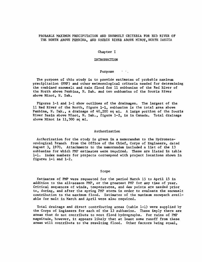
Narrative meteorological discussions are given here for transposed storms that provide the greatest adjusted rainfall depths (see chapter 3) over the Red River of the North and Souris River drainages.

Most of the storms come from the catalogue of maximum areal storm rainfall depths (Corps of Engineers 1945-). A survey was made of Canadian storm rainfall (Atmospheric Environment Service 1961) for those transposable to the basins. A comparison of these with transposed u.s. storm rainfall showed the latter depths were greater for all area sizes and durations of concern. A search of climatological records was made for other large-area storms that might be helpful in setting the level of PMP. Some storms were found and maximum depth-area-duration (DAD) values of rainfall computed. In developing all-season PMP, two of these (identified with a number preceded by HMB in the following headings), gave greater adjusted depths for certain area sizes and durations than any in the catalogue of United States storm rainfall (Corps of Engineers 1945-).

Each storm in the following summary is identified by the date of the rain­fall, location of the rainfall center and the Corps of Engineers Assignment Number or Hydrometeorological Branch number. The combined adjustment for moisture and transposition to the Red River of the North is given near the end of each summary narrative. Figures 2-la and 2-lb show the center of heaviest rainfall by an "x" and an outer isohyet for each storm. These are numbered and added to the end of the storm identification.

July 18-21, 1897- Lambert, Minn. (UMV 1-2), Figure 2-la, No.1

Weather maps for this early storm and discussion in the Monthly Weather Review indicate the heaviest bursts of rain occurred on July 20 while a quasi-stationary low centered in southeastern South Dakota was intensifying. The greatest measured rainfall was at Lambert, Minn. where 8 in. fell in a little over 2 days. The low then moved across central Minnesota during the night of July 20 before turning toward the northeast on July 21. Rainfall was well centered over the Red River of the North Basin. This storm is important for extreme rainfall over large areas (50,000 sq mi) for short durations. The storm adjustment is 148 percent (48-percent increase).

June 9-10, 1905- Bonaparte (nr), Iowa (UMV 2-5), Figure 2-la No. 2

An unusually large high pressure center over the Great Lakes on June 8 slowly shifted to the southeast, reaching Cape Hatteras by June 10. The return flow from the south around this high was an important feature for bringing in warm, moist air from the Gulf of Mexico.

6

A low had developed over Wyoming on the 8th, This moved east to the northeast corner of Nebraska by 6 a.m. of the 9th and to southeast Iowa by 6 a.m. of the lOth, A strong pressure gradient between the high and low was responsible for northerly transport of warm, moist air. A wave on a warm front on the northern bound of the warm air reached Nebraska by a.m. of the 9th. Relatively slow movement of the anticyclone and low associated with the wave concentrated the rain to give a little over 12 in. of rain near Bonaparte, Iowa, between evening of the 9th and morning of the lOth. Convergence associated with the low was the primary factor causing the heavy rain. The storm adjustment is 128 percent.

July 18-23, 1909- Beaulieu, Minn. (UMV 1-lla), Figure 2-la, No. 3

A low formed over South Dakota on July 19 in an eastward-moving low pressure trough. This low moved slowly to the north-northeast, The heavy burst of precipitation (12 in. in 60 hr) centered at Beaulieu, Minn., late on July 19 occurred ahead of a warm front associated with this low, while farther east at Ironwood, Mich., heavy rain occurred on July 21-22 in the warm sector of the low. The rainfall associated with the western center was the greatest, and only the western half of the total isohyetal map is used for this study. A strong inflow of moisture was augmented by the circulation of a tropical storm along the Gulf coast. A cold-front passage between July 21-22 ended the precipitation. Storm adjustment is 134 percent.

June 1-6, 1917- Atlantic, Iowa (MR 2-16), Figure 2-lb, No. 4

Thunderstorms, associated with two occluded frontal systems that moved northeastward across Iowa during June 1-6, produced the important rainfall for this period.

On the morning of June 1, a trailing cold front extended from a low near the Great Lakes southwestward to Texas. Warm gulf air circulated around a bulge of high pressure over the Southeastern States. During the day cyclogenesis occurred on the front in a low in Texas. The resulting wave rapidly moved northeastward and occluded over Iowa. This system produced the severe thunderstorms between evening of the lst and 6 a.m. of the 2nd. Rain ceased with the passage of the occluded system to the northeast.

Following a high-pressure center moving northeast out of the area on the 3rd, a circulation of warm gulf air was reestablished. The approach of a new cold front from the north (3rd and 4th) to Iowa over which warm gulf air was lifted caused thunderstorms primarily during the evening of the 4th. The front progressed slowly southward allowing additional thunderstorms on the evening of the 5th over the same area. The rain ceased as a stronger push of cold air spread over the area on the 6th. Storm adjustment is 171 percent.

7

September 17-19, 1926- Boyden (nr), Iowa (MR 4-24), Figure 2-lb, No. 5

A well-defined cold front in a NE-SW-oriented trough of low pressure with high pressure centers to the northwest and southeast advanced into southeastern South Dakota by the morning of September 17. Continued south­eastward movement set off heavy showers and thunderstorms in the warm, moist air flowing northeastward over northwest Iowa on the afternoon and evening of September 17. Maximum observed rainfall was 24 in. in 18 hr • Clearing took place as cool,dry air moved in the following passage of the cold front. Storm adjustment is 122 percent.

June 3-4, 1940- Grant Township, Nebr. (MR 4-5), Figure 2-la, No. 6

The Bermuda High extended well over the central East Coast States for several days prior to June 3. Southerly flow on the western side of this high brought warm, moist and convectively unstable air from the gulf as far north as Nebraska and Iowa. A trough of low pressure oriented almost north­south near the eastern border of Colorado on the 3rd moved eastward to central Nebraska by the morning of the 4th. The cold front approaching from the northwest set off heavy showers and thunderstorms in the warm air on the afternoon and night of June 3. The greatest measured rainfall was 13 in. in 6 hr • Almost 9 in. occurred over 1000 sq mi in 12 hr • Weather maps indicate northward movement of a small wave along the front was instrumental in positioning the heavy rainfall. The storm adjustment is 148 percent.

August 12-16, 1946- Collinsville, Ill. (MR 7-2b), Figure 2-lb, No. 7

A mass of cold air covered most of the Eastern and Central United States, except Florida and most of Texas, on the morning of August 12. One of a number of waves in l'lyoming and Colorado on the boundary of this cold air mass moved eastward, causing heavy precipitation between the evenings of the 12th and 14th over eastern Kansas and much of Missouri. Unstable, warm, moist air from the Gulf of Mexico in the warm sector of the wave overrunning the cold air to the northeast caused the general rains. This warm-frontal rain advanced into southern Illinois on the night of August 14, ending with the passage of the warm front. Heaviest showers of the storm period then broke out in the warm sector of the wave on the night of August 15-16. Maximum station rainfall was close to 19 in. in 3 days. Drier air came in aloft and the showers decreased in intensity and ended following passage of a cold front on August 18. Storm adjustment is 116 percent.

July 9-12, 1951- Council Grove (nr), Kans. (MR 10-2), Figure 2-lb, No. 8

The meteorology of this sto~important for long durations over large areas, both where it occurred and when transposed, is discussed in detail in Weather Bureau Technical Paper No. 17 (U.S. Weather Bureau 1952b), and is summarized here. Beginning with the 9th and through the 12th, high pressure persisted in the North Central States, extending south to near the Kansas-Oklahoma border. A weak low at the same time persisted in New

8

Mexico. This situation set up a strong east-west pressure gradient through Texas and Oklahoma resulting in strong northward flow of warm, moist air into the heavy rain area. A particularly strong surge of cold air on the lOth forced upward motion of the moist air and heavy rainfall in Kansas. The strong inflow of moisture, the energy associated with the high tempera­ture contrast, the instability of the warm air, and the fact that the frontal boundary between the cold and warm air remained nearly stationary for several days are apparent factors contributing to the heavy rain. Storm adjustment is 122 percent.

Transposition limits determined for Technical Paper No. 17 extend to the southeast corner of the basin. These limits have been extended in the present study to include the entire Red River of the North. This extension was based on consideration of the meteorology of some additional storms investigated as part of an ongoing study of generalized PMP estimates for large basins. These storms were not considered in developing the limits set in Technical Paper No. 17.

June 7-8, 1953- Ritter, Iowa (HMB 6-53), Figure 2-la, No. 9

A cold air mass preceded by a cold front moved southward over the North and Central Plains States a few days before the heavy rainfall. A low­pressure center formed on the front in Colorado on the morning of June 7. This low deepened and moved quickly northeastward to east-central Minnesota by the morning of June 8, then continued east-northeastward into Canada. Very heavy 'ains occurred in thunderstorms ahead of the warm front and in the warm sector as the low moved across northwest Iowa the latter half of June 7. The 700-mb charts prior to and during the storm showed strong south~ erly moist flow from the Gulf of Mexico around a westerly extension of the Bermuda High. A cold front moving southeastward following passage of the low center ended the rain. Storm adjustment is 155 percent.

September 11-13, 1961- Shelbina, Mo. (HMB 9-61), Figure 2-la, No. 10

Moisture associated with Hurricane Carla was responsible for the large area of heavy rainfall on September 11-13 centered in northeast Missouri. The 4-in. isohyet extended from Oklahoma to Lake Michigan. Carla crossed the gulf coast approximately 70 mi northeast of Corpus Christi in the later hours of the 11th with a northwesterly heading. Shortly thereafter the storm took a northerly course,reaching the southern border of Oklahoma by 1 a.m. of the 13th. By 1 p.m. the tropical storm merged with a cold front, then moved northeast to Lake Michigan by 1 a.m. of the 14th as a low on the front. Heaviest rains occurred well ahead of the storm center from the evening of the 12th to noon of the 13th while the tropical storm was changing to a northeasterly track. The deep northerly flow of moisture (surface dew points were within a few degrees of the maximum 12-hr persisting dew points for September near the gulf coast) moving upward over the cold front and convergence of the moist air about the low center produced the heavy rain­fall. Storm adjustment is 105 percent.

9

>-' 0

100°

... X-storm center. No. near center identifies storm (see chapter 2), T __ L_ ____ _

r------1 ,..! i I ~ I 1000 '--~-

95" 90" +

soo+ .,.

' I

r '? ) '"'-. ;--

r------)__/Y~-+ I ~---""-, , I

--9.!."1 I I' ! 90° . '

Figure 2-la.--Outer isohyets of storms important to PMP for the Red River of the North and the Souris River drainage basins.

11i5° .... +50"·' ' (""JSOURI?- + + '-,. _RIVER t ~-, '\

100° w '!" 0 "'"'""', J - 1 ' -......,

-~r BASIN,---.!.,__.._~- __j \

\ \ ,. BASIN OF'-.., --· , "~ j RED RIVER -, --.../'--/ <.,_;--...\OF THE _NORTH,.,.,.;>

I \ \ ~ L i \ t ' --------\,-' (

-..( J ·45°~ + :-'

' I

X-storm center, No. near center identifies storm~­(see chapter 2),

95"

50°+ 85"

' I

Figure 2-lb.--Outer isohyets of storms important to PMP for the Red River of the North and the Souris River drainage basins.

Chapter 3

ALL-SEASON PROBABLE MAXIMUM.PRECIPITATION

Method of Estimating PMP

The method in most general use for estimating probable maximum precipitation (PMP) in the United States where topography has little or only a minor influence may be termed the moisture-maximization transposition procedure. This has been used in the present study for estimates of all-season and springtime PMP. The method can be summarized by the following three steps:

1. Moisture maximize the greatest areal storm rainfall depths that have occurred in the meteorologically homogeneous region surrounding the drainage area under study by adjusting them to the highest atmospheric moisture observed in the region. In practice, surface dew points are used to obtain the moisture adjustment factor because of lack of upper-air soundings in early storms, and because there is a much more dense network of surface dew-point observations than of upper-air observations. The storm 12-hr persisting dew point representative of the moisture inflow is reduced pseudoadiabatically to 1000 mb and the precipitable water computed in a saturated air column with that 1000-mb dew point value. A moist adiabatic lapse rate is assumed. The maximum precipitable water is obtained in a similar way, based on the maximum persisting 12-hr 1000-mb dew point (Environmental Data Service 1968) within 15 days of the date of the storm. The ratio of the maximum to the storm precipitable water is the moisture adjustment factor by which maximum observed storm depth-area-duration rainfall values are multiplied.

2. Transpose maximized storm rainfall depths to the basin. Transposition requires identifying the type of storm and isolating the factors important to heavy rain. A survey of weather charts will help to delineate the region within which a particular storm type has occurred. The climatology of storm tracks frequently is additional guidance. In transposing a storm, a relocation adjustment is applied. This is the ratio of the maximum persisting 12-hr 1000-mb dew point in the transposed location to that where the storm occurred.

3. Envelop transposed and maximized storms. Smooth envelopes of the adjusted storm rainfalls are made with duration for selected area sizes. Thus, maximized depths for two durations, for example, 2~and 72-hr, from two different storms when enveloped with a smooth curve, may determine the depths for intermediate durations. Similar smooth envelopes are then made across area for each duration.

11

The basic concepts in this method can be summari.zed as follows: All factors conducive to heavy rain, except moisture, may be termed storm "mechanism." If there are sufficient transposed major storms, it is assumed maximum or near-maximum values of storm mechanism have been experienced such that with moisture maximization an estimate of the rainfall potential is obtained.

Some discussion of the moisture maximization procedure is covered in Hydrometeorological Report No. 33 (U.S. Weather Bureau 1956). Technical Hemorandum WBTM HYDR0-5 (Myers 1967) discusses the several steps of this method for obtaining PMP.

Storms Processed and PMP Estimates

"Storm Rainfall in the United States" (U.S. Army Corps of Engineers 1945-) and its counterpart in Canada (Atmospheric Environment Service 1961) were the basic sources of storm data. Because these contain relatively few large-area storms, a survey was made of the precipitation amounts in "Climatological Data for the United States by Sections" (U.S. Heather Bureau 1970) for additional storms that would appear to provide critical rainfall depths. Some critical rainfall periods were found and preliminary storm rainfall values computed for each. Two of these storms were important in setting the level of PMP~ Table 3-1 lists the major storms considered. The last two columns of the table give the combined adjustment for moisture maximization and transposition to the centers of the Red River of the North and Souris River Basins, respectively.

Adjusted storm depths for each basin were plotted on semi-logarithmic paper and smooth enveloping depth-area curves drawn for each duration, figure 3-1. Further smoothing was obtained for selected standard size areas by means of depth-duration plots (not shown).

The storms that are controlling or near-controlling (that is, those giving the greatest depths for particular area sizes and durations) for either of the two basins are marked with an asterisk in table 3-1. Figure 2-la and b show the centers of these storms and outer isohyets. Table 3-2 lists the controlling storms for standard areas and durations.

Figure 3-1 gives enveloping PMP for the center of the Red River of the North by the solid curves. A separate set of curves (not shown) were prepared for the Souris River Basin. Comparison of the enveloping DAD curves for the centers of the Red River of the North and Souris River Basins shows relatively small differences. A 10-percent reduction of the Red River of the North envelopes reproduces the independently determined Souris River DAD envelopes without significantly overenveloping or undercutting adjusted data. Therefore, a basic PMP estimate for a Souris River subbasin may be obtained by taking 90 percent of PHP for the Red River of the North. Geographic variation within basins is obtained from figures 4-2 and 4-3.

12

Dashed curves of figure 3-1 are depth-area curves used in distributing PMP within basins. Their development and use are discussed in chapter 5.

Comparison With Other PMP Estimates

A PMP study for an adjoining drainage, the ~linnesota River (U.S. Weather Bureau 1969), provides a test for consistency with the present estimates. Bett<een 1,000 and 10,000 sq mi, Red River of the North estimates are 2 to 8 percent lower. At the 20,000-sq-mi area, the Red River of the North estimates are 10 percent greater for 6 hr and down to 2 percent greater at 72 hr. The additional storm rainfall data from the storm search in the present study and some variation in degree of envelopment account for these increases.

A study (U.S. Heather Bureau 1952c) for portions of the Red River ~<as made in 1952. Basic enveloping PMP values in that study were determined for areas up to 5, 000 sq Tili. PMP estimates for 6 hr in that report are the same as in this study for 1,000- to 5,000-sq-mi areas. For longer durations, this study is higher; by 10 percent for 24 hr and up to 28 percent for 72 hr. Most of these differences are due to unavailability of the July 1951 Council Grove, Kans., storm (MR 10-2) rainfall depths for the earlier estimate.

Generalized PMP for areas up to 1,000 sq mi and durations to 48 hr (U.S. Weather Bureau 1956) are in good agreement with the present study. For large areas, a current study giving tentative generalized estimates of all-season PMP in the Central and Eastern States shows approximately the same values as given here.

13

Table 3-1.--Major storms considered for Red River of North and Souris River Basins all-season PMP

Storm adjustment Assignment (percent)

number Storm date Storm center Red River Souris of North River

*UMV 1-2 July 18-21' 1897 Lambert, Hinn. 148 141

MR 1-5 July 14-17, 1900 Primghar, Iowa 128 122

UMV 1-6 Sept. 7-11, 1900 Elk Point, S. Dak. 122 116

MR 1-10 Aug. 24-28, 1903 Woodburn, Iowa 116 100

GL 2-12 June 3-7, 1905 Medford, Wis. 122 110

*UMV 2-5 June 9-10, 1905 Bonaparte (nr) , Iowa 128 116

UMV 2-18 Sept. 12-19' 1905 Boonville, Mo. 141 116

MR 5-13 June 6-8, 1906 lvarrick, Mont. 189 189

*UMV l-11a July 18-23, 1909 Beaulieu, Minn. 134 128

MR 4-14a June 25-28, 1914 Hazelton, N. Dak. 134 128

*MR 2-16 June 1-6' 1917 Atlantic, Iowa 171 156

MR 4-21 June 17-20, 1921 Springbrook, Mont. 128 128

*MR 4-24 Sept. 17-19' 1926 Boyden (nr) , Imva 122 110

MR 5-2 June 6-8, 1934 Akron, Iowa 171 163

*MR 4-5 June 3-4, 1940 Grant Township, Nebr. 148 127

UMV 1-22 Aug. 28-31' 1941 Hayward, Wis. 134 122

MR 6-15 June 10-13, 1944 Stanton (nr), Nebr. 128 116

SASK 7-46 July 9-10, 1946 Rhodes Ranch, Mont. 171 163

MR 7-Za Aug. 12-15, 1946 Cole Camp, Mo. 116 105

*MR 7-Zb Aug. 12-16' 1946 Collinsville, Ill. 116 105

*MR 10-2 July 9-12, 1951 Council Grove (nr) , Kans. 122 110

*HMB 6-531 June 7-8, 1953 Ritter, Iowa 155 141

*HMB 9-611 Sept. 11-13, 1961 Shelbina, Mo. (CARLA) 105 90

*Controlling or near-controlling all-season PMP. !Preliminary DAD data by Hydrometeorological Branch.

14

Table 3-2.--0bserved rainfall (in.) for controlling or near-controlling storms, all-season PMP Red River of the North

Duration Area (sq mi) (hr)

1,000 5,000 10,000 20,000 50,000

6 9.2 5.8 4.4 2.5 1.4 (UMV 1-lla) (UMV 2-5) (UMV 2-5) (HMB 6-53) (MR 2-16)

12 8.9 6.1 4.8 3.5 2.3 (MR 4-5) (HMB 6-53) (HMB 6-53) (HMB 6-53) (UMV 1-2)

18 6.8 5.6 4.2 2.9 (HMB 6-53) (HMll 6-53) (HMB 6-53) (UMV 1-2)

24 6.1 4.7 (liMB 6-53) (IDIB 9-61)

36 14.7 10.4 5.3 (MR 7-2b) (MR 7-2b) (HMB 9-61)

60 15.9 11.7 10.4 8.6 (MR 7-2b) (MR 10-2) (MR 10-2) (HR 10-2)

72 15.5 13.0 11.4 9.4 (MR 10-2) (MR 10-2) (MR 10-2) (MR 10-2)

15

100 80 60 50 40 30

- 20 "' = ~

~ 10 0 0 8 .. 6

>-' ~ ~ 5 "' ..

4 3

2

1 .8

.6

. 5

.4

.3

.2

.12

Date Number -

1 18-21 July 1897 2 9-10 June 1905 3 18-23 July 1909 4 1-6 June 1917

~,~.,, 5 17-19 Sept 1926 " ' 6 3-4 June 1940

' 7 12-16 Aug 1946 ' ' 8 9-12 July 1951 ' ' ' 9 7-8 June 1953 ' ' 10 11-13 Sept 1961 ' \

\ \ '· \ \ I \

\ \~ \

\~ \

\~ \~ \-., \~

~ \~ \~ \

1.,. I~ , __

Storm No. I'? \ '· \~ I~ \~' ,~ • \~ \~ Duration (hr) \~ '"'

\~

I~ \·~ I ~ I"' I I '"' I I I~ I I ,-I I ,~

I I \~ I I

4 6 8 10 12 14 16 18 -. 20 22

Figure 3-1.--Enveloping depth-area-duration values of P11P for the center of the Red River of the North above Pembina, N. Dak.

Chapter 4

SEASONAL AND GEOGRAPHIC VARIATION

Seasonal Variation

For determining the maximum flood from combined snowmelt and a rainstorm, it is necessary for this region to define PMP for the primary snowmelt months, March and April. There are an insufficient number of severe storms in these months so that a direct approach (moisture maximization, transposition, and envelopment), as was used for all-season PMP, will not give reliable PMP estimates. Other precipitation indices used as guidance in determining the recommended seasonal variation are described in the following paragraphs. Figure 4-1 summarizes the indices.

Month of Highest PMP

Station maximum 1-day precipitation of record, useful in determining seasonal variation at least for small areas, indicates the all-season PMP can occur as early as June in the region of these drainages. Station maximum precipitation for the U.S. was obtained from Weather Bureau Technical Paper No. 16 (U.S. Weather Bureau 1952a). It covers the period of record through 1949. Maximum station precipitation for Canada comes from (Department of Transport 1958). Table 4-1 shows which months contributed the greatest 1-day rains at 206 stations with long records in states or provinces near the drainages. Only one station with a long record had its annual maximum outside the April-October season. This is Crosby, N. Dak. (4.02 in., Nov. 7, 1915). June contributed the greatest number, 70, with 48 for July and 46 for August.

Four of the 10 storms most critical for the all-season PMP (table 3-1), occurred in the first part of June. These are the storms of June 9-10, 1905 (UMV 2-5); June 1-6, 1917 (MR 2-16); June 3-4, 1940 (MR 4-5); and June 7-8, 1953 (HMB 6-53). Of the remaining six storms, three occurred in July, two in September, and one in August.

It is concluded the all-season PMP can occur as early as June 1.

Station Precipitation as Guidance to Seasonal Variation

The highest 1-day precipitation values for February through June at stations with 30 or more years of record in Minnesota (north of 46° latitude) and North Dakota were extracted from published summaries (U.S. Heather Bureau 1952a). The ratio of the highest 1-day value for each month to that for June was computed for each station. The resulting station average ratios, or average percents of June, for each state are shown by the crosses in figure 4-1. Highest average percents of June are: February 37, Harch 47, April 63, and May 84.

17

Other Indices

Variation of maximum moisture is an index to be considered in the variation of PMP. The seasonal variation of moisture over the drainages, as determined from maximum persisting 12-hr dew points (Environmental Data Service 1968) and expressed in percent of moisture in June, ranges from 23 percent in February to 73 percent in May.

Another clue to seasonal variation of precipitation is temperature contrast, which represents potential energy subject to transformation into kinetic energy. As a qualitative index to temperature contrast, the maximum 1000-to 700-mb thickness gradient within 300 mi of Fargo obtained from normal maps (U.S. Weather Bureau 1952d) is plotted in percent of mid-June on figure 4-1. Expressed in percent of June values, the highest percentage (167) comes in February, with a smooth decrease in the monthly percentages to June. Combination of moisture and temperature contrasts, by multiplication of corresponding monthly values, results in a seasonal variation not too different from that of maximum station precipitation. It progresses from 35 percent of June in February to 83 percent of June in Hay.

The recommended seasonal variation and supporting data are shown in figure 4-1. The adopted variation is somewhat above the average percents of June for 1-day maximum precipitation. Percents of all-season PMP taken from the figure for !1arch and April are shm;n in table 4-2.

Geographic Variation

There is variation in PMP within each basin, largely because of the distance from moisture source. Other factors remaining constant, rainfall decreases as the distance from the Gulf of Mexico increases. For this study, the variation was developed from !frill No. 33 (U.S. Heather Bureau 1956) and a tentative variation from an ongoing large-area PMP study for the eastern two-thirds of the United States. A compromise between the two studies was adopted. Geographic variation from the two mentioned sources gives somewhat different values from the adopted 90 percent of the Red River of the North for the Souris River Basin. However, it is considered acceptable within the limitations of the data. Geographic variation for March, April, and June is given in figures 4-2a to c for the Red River of the North Basin and figures 4-3a to c for the Souris River Basin.

On each map, 100 percent is drawn through the center of the basin, the location for which the PMP was determined and to which the seasonal variation applies.

18

Table 4-1.--Month in which greatest 1-day station precipitation of record occurred

(U.S. stations with 30 or more yr of record; Canadian stations with 10 or more yr)

Number of stations with greatest 1-day Number precipitation in indicated month

State or province of stations

Apr. May June July Aug. Sept. Oct.

Minnesota (north of 46° lat.) 41 0 2 6 12 15 5 1

Montana (east of I l09th meridian) 27 I

1 4 12 5 2 3 0

North Dakota 77 I 2 8 30 16 14 5 1 I ' I

Saskatchewan 26 I 0 3 10 7 5 1 0 I

'

Manitoba 35 i 0 3 12 8 10 1 1

---206 3 20 70 48 46 15 3

Table 4-2.--Recommended seasonal variation of PHP

(Percent of all-season values, fig. 3-l)

Date Percent

Nar. 1 45

Mar. 15 53

Apr. l 62

Apr. 15 72

19

180.---------------.,

.,. ... = ..... cc > ...

160

140

120

:z: 100 ~

.... C>

!Z 80 ... c.:> ... ... ....

60

20

2

FEB

•

•

•

RECOMMENDED VARIATION FOR PMP

0

MAR

+1 N. Dak. (77 stations)

+2 Minn. (41 stations)

• Maximum 1000-700 mb thickness gradient

o Seasonal variation of moisture

x Product of thickness gradient and moisture

APR MID-MONTH

MAY

Figure 4-1.--Adopted seasonal variation of PMP and supporting data.

20.

JUNE

., . ... ... ...

•.

+ ., . .;:-;_ ... '.~· .... ·, .,.

• .••,C&MAOA

..

.,.

MU><8ERS "'THIM ... lJM

"'- ·-..c,-~~ 1211:."~}~~c!.~ROJE<T liEf TA8\.E 1-11

+ •. .,. ITATUHO<Jl[l

,. "' " ., "' 100" •• ... ...

Figure 4-2a.--Geographic variation of PHP. Red River of the North. March.

.,. ... ...

MINNESOTA

.. .

+

H'-"'BERIWIIHIM8A1JM IDEMTIFT POOJECI lDOTIDN'

"EET .. LE 1.11

.,.

""+ + •. lOUTH OA.OH +

n,UUIE"'l"

10 , "' ., "'

IOO" ... ... ... Figure 4-2b.--Geographic variation of PHP.

Red River of the North. April.

21

" .,. ... ., . ...

- +-- .. -----+-·-- ___ .9'

NORTK

CLOSED BASIN

.,. ,,. l(ll•

""\·I:~:J~\ '"":.:.,.....,;:;;'5':','.:'\.~~ -­-~,_-. l-~:o~~m -:>

~OATH QUOTA\ )

- )

MINNESOTA

+

~U~BEIIS .,THIN~~~

IDENTIFY POOJEC:l L<>CATI0r<l

IIEETAioi.E 1.11

.,.

'''+ ~UT~ D .. OH + •.

100' ... ... .,.

Figure 4-2c.--Geographic variation of PMP. Red River of the North. All season.

10~· 104'

lOS'

... +•I' +

lOUTH DUOU

101•

'"

NUMBERS WITHIN BASI!i IOENTIFY PROJECT LOCA.TIONS

I SEE TABLE 1-11

... +

'" H .. lUTE "ILEI

'""

+

101'

..

Figure 4-3a.--Geographic variation of PMP. Souris River. Harch.

22

NUMBERS WITHIN BASIN ID~HTIFY PROJECT LOCATIONS

(SEE TABLE 1-1) ... IOINHE~OTA

... + + SOUT" OA~OTA

" • • , ... ''"

STATUTE IOI~ES

'"

Figure 4-3b.--Geographic Souris River.

variation April.

105"

..

105"

... ,,.

• ~OUT" OUOU

·~

104"

•••

''"

NUMBERS WITHIN BASIN IDENT1H PROJECT LOCATIONS

(SEE TABLE 1-1)

... +

""

+

1020)1l.O~

'"' ""

...

of PMP.

'"

...

Figure 4-3c.--Geographic variation of PMP. Souris River. All season.

23

Chapter 5

TIME AND AREAL DISTRIBUTION

In determining a flood hydrograph, the magnitude of the flood is often dependent on the manner in which a given precipitation volume (average depth over the area) is distributed. Also, the degree of concentration of precipitation with time during a storm and the sequence of incremental precipitation values for short time periods are important considerations. In this chapter a procedure is suggested for the time and areal distribution that is patterned after major storms, essentially maintains PMP magnitude for all durations, is relatively simple, and will result in consistency among the subbasins.

Time Distribution

It is assumed that a single storm can produce PMP for all durations over a subbasin. Therefore, basic all-season PMP for all durations for a sub­basin may be read from figure 3-2, at the area of the subbasin. These values are then adjusted for location and season. Six-hour PMP increments from the greatest (1st) to lowest (12th) are obtained by successive sub­traction after drawing a smooth durational curve of rainfall through the accumulated adjusted values.

Having determined the 6-hr rain increments, the question remains of how these should be sequenced relative to each other in the PMP storm. Inspec­tion of many storm mass rainfall curves shows a wide variety of possible sequences. One fairly consistent pattern is for bursts to last from 6 to 18 hr with lulls between them. Such sequences, followed closely, will not yield the required PMP values for each duration from 6 to 72 hr • A compromise between the storm mass curve indications and the desirability for maintaining PMP for all durations is to apply the following guidelines:

1. Group the four highest 6-hr increments of the 72-hr PMP in a 24-hr period, the middle four increments in a 24-hr period, and the lowest four increments in a 24-hr period.

2. Within each of these 24-hr periods,arrange the four increments in accordance with the sequential requirement for maintaining PMP. That is, the second highest next to the highest, the third highest adjacent to these, and the fourth highest at either end.

3. Arrange the three 24-hr periods ·with the second highest 24-hr period next to the highest and the third at either end. Any possible sequence of three 24-hr periods is acceptable with the exception of placing the lowest 24-hr period in the middle.

24

Areal Distribution

It is assumed uniform areal distribution may be used for all 6-hr PMP increments over drainages of less than 1,000 sq mi. For larger areas, we recommend distribution of the two greatest 6-hr PMP increments by a hypo­thetical isohyetal pattern. The remaining PMP increments may be distributed uniformly, that is, one average depth for the drainage.

Shape of Isohyetal Pattern

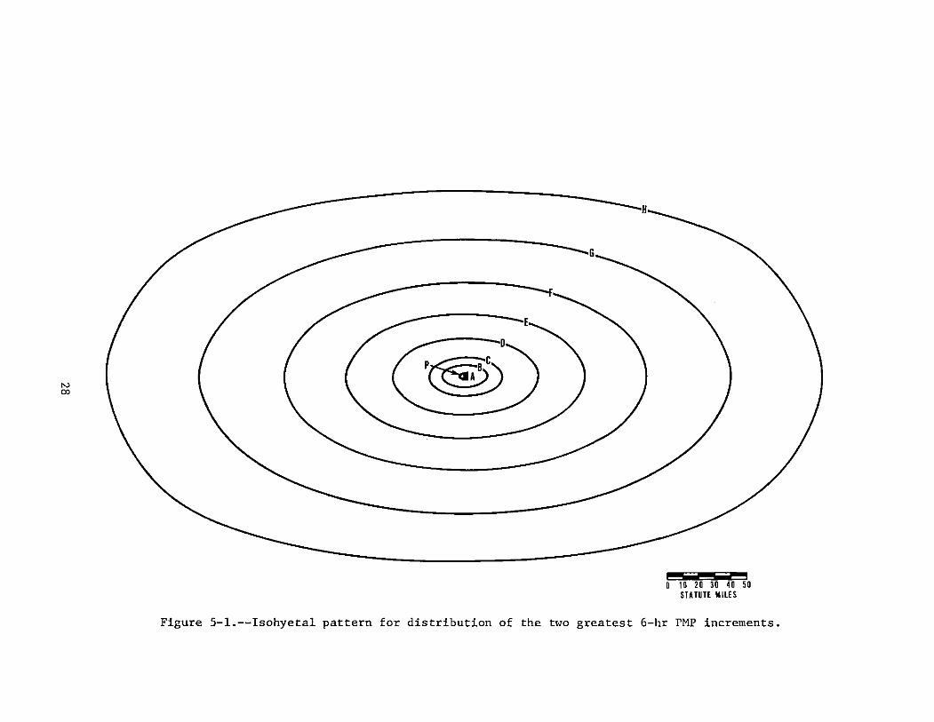
One consideration in areal distribution is the shape of the isohyetal pattern. Unless a subbasin outline is quite elongated or irregular it is reasonable to assume the isohyets could essentially conform to the outline. For this study, we suggest the elliptical isohyetal pattern shown in fig­ure 5-l. This pattern has a major-to-minor axis ratio of 2 to 1. Table 5-l gives the areas of the isohyets in the pattern.

Computations were made to check the reduction in rainfall that would result from differences in the shape of the pattern and subbasin shapes. For an extreme case, the contributing drainage area (1,910 sq mi) of the Sheyenne River above Baldhill Dam, N. Dak., the reduction is 25 percent for the greatest 6-hr period and 10 percent for the second greatest. Similar reductions were computed for the Sheyenne River above Kindred, N. Dak. (drainage area 3,020 sq mi). Generally, reductions between 5 and 10 percent resulted for the remaining subbasins.

Orientation of Isohyetal Pattern

In a study for the Tennessee Valley Authority, Schwarz (1970) found a relation between the magnitude of 3-day rains and the orientation of the isohyets. Direction of flow of moisture from its source region relative to upper-air steering currents in major storms tended to produce greater rainfall volumes in certain isohyetal orientations. A similar study was carried out for the region of the present study. A number of storms from Storm Rainfall (u.s. Army Corps of Engineers 1945-) with isohyets extending into North Dakota, South Dakota, Minnesota, Wisconsin, Nebraska, Iowa, and northern Illinois were considered as well as Canadian storms (U.S. Army Corps of Engineers 1945-) in the southern half of eastern Saskatchewan, Manitoba, and western Ontario. This gave an average of 95 storms for 72-hr duration for which the orientations of the isohyets and rainfall depths for numerous area sizes, from 5,000 to 20,000 sq mi, were correlated. One extreme depth for a storm with an isohyetal pattern extending into Iowa and southern Minnesota but centered in Oklahoma, has far greater depths than the more northerly storms for large areas with nearly a north-south (20") isohyetal orientation. Because the storm was centered farther south than the others, it was not given full weight. Envelopment and compositing of greatest rain depths plotted against orientation of major axes of isohyets

25

showed maximum values for orientations between 20° and 100° from the north, Figure 5-2 is an example of the data for 72-hr duration for 20,000 sq mi with the adopted variation. This variation.in rain depths with isohyetal orientations is also shown in table 5-2. Orientations other than those listed, if needed, may be obtained by interpolation.

Isohyetal Values

For smaller areas within the total area of a subbasin, we recommend an areal rain distribution that falls between using uniform distribution and assuming PMP for all area sizes within the subbasin, Depth-area relations giving such areal distributions are shown by dashed lines at key areas and dura­tions on figure 3-2. These were derived from rainfall depth-area relations of major storms in the region of the basins. For identification purposes they are termed "within basin" depth-area curves, For example, the "within basin" depth-area curve shown for 6-hr duration for basin sizes of 10,000 sq mi or more is a composite of depth-area relations in major storms of the region that had controlling or near controlling 6-hr depths for 10,000 sq mi. It was found that this curve is representative of storm depth-area relations for area sizes up to 50,000 sq mi. The 6-hr curve for 1,000-sq-mi basins is the average depth-area relation of controlling storms for that duration and area size. Depth-area curves (not shown) were also determined in a similar way for 5,000-sq-mi basins.

A full family of "within basin" depth-area curves were derived for area sizes from 1,000 to 10,000 sq mi for the greatest and second greatest 6-hr PMP increments by interpolating between the sets for 1,000, 5,000 and 10,000 sq mi or greater. Then nomograms were computed relating percent of PMP for basin sizes to areas of isohyets. These nomograms are shown in figures 5-3 and 5-4 for the greatest and second greatest 6-hr PMP increments. They will give consistent isohyetal labels for drainages up to 40,000 sq mi in area.

For the remaining ten 6-hr PMP increments, uniform areal distribution may be used,

Chapter 8 outlines a procedure for using the nomograms of figures 5-3 and 5-4, as well as the geographic and seasonal adjustments.

26

Table 5-1.--Areas of pattern storm isohyets (fig. 5-l)

Isohyet Area (sq mi)

p 10 A 35 B 270 c 800 D 3200 E 8700 F 19700 G 42300 H 76600

Table 5-2.--Variation in PMP with orientation of isohyetal pattern

Orientation of major axis from north

10°

zo•} to

100°

120°

140°} to

18o•

27

Percent of basic PMP from fig. 3-1

95

100

95

87

N OJ

p®

0 10 20 30 40 50 STATUTE MILES

Figure 5-1.--Isohyetal pattern for distribution of the two greatest 6-hr PMP increments.

20,000-sq-mi rainfall for 72 hrs

10~ • u.s. storms -X Canadian storms

•!STORM CENTERED IN OKLAHOMA)

--:z:

:z: • = X • • ;::: 6 • -c X • X N !:: • • "' !!::: X •• • ... X • X • X •• .... • • • ... • • • • XX • .... X • X • • • X X • • • 4 X • X -• ~ • • • • • X ~ I X • • • • •• • x: X • • X XX •• • • • • •• X

X • • 21

X -• ORIENTATION OF MAIOR AXIS OF ISOHYET )FROM NORTH)

0 20 40 60 80 100 120 140 160 180

Figure 5-2.--Example of variation in rainfall with isohyetal orientation.

H G E D p

IO~_J~~--~--~~~~~Lh--~~h-~~~~~~~~h-~~~~~~~~h-~~~~~~~~h--" 1B 20 40 tiD 80 100 120 140 160 180 200 220 240 260 280 300 320 340 360 380 400 420 440 460 480 500

PERCENT OF PMP AT AREA Of BASIN

Figure 5-3.--Nomograrn for determining isohyet values for greatest 6-hr P~W increment.

;;:

= ~

~

= = =-:: ~

c z ;:;; ;::

H

100

10 o~---2~0~~40~~60~~8~0--~IOU0--712h0~~,~40~~~~~~~~~~2~40~~2~6~0~2~8~0~JOO PERCENT OF PMP AT AREA OF BASIN

Figure 5-4.--Nomogram for determining isohyet values for 2nd greatest 6-hr PMP increment.

30

Chapter 6

SNOWMELT CRITERIA

Introduction

This chapter presents critical sequences of temperatures, dew points, and winds that can accompany the spring PMP storm. Criteria are given for the storm period (part A); for 10 days prior to the storm (part B); and for 3 days after the storm (part C). Other considerations required for computing snowmelt such as amount and type of forest cover and radiation are not a oart of this study. Critical snowpack for spring melt is covered in chapter 7.

A. Temperatures and Windspeeds During the PMP Storm

Dew Points

Dew-point temperatures for occurrence with the spring PMP storm are based on maximum persisting 12-hr 1000-mb dew points (Environmental Data Service 1968) over each basin. From Weather Bureau Technical Paper No. 5 (U.S. Weather Bureau 1948), the durational variation in persisting d~• points was computed for 4 stations near the two basins for March and April. Differ­ences in values between stations and between the two months were not significant; therefore, one variation was adopted. This average is shown in percent of the precipitable water (associated with the persisting dew point for each duration) for 12 hr , in table 6-1.

Maximum 12-hr dew points vary sufficiently over the basins so that they should be specified for the location of a particular subbasin being studied. Figures 6-1 and 6-2 are maps of the maximum persisting 12-hr dew points for March 15 and April 15. Figure 6-3 shows the relation between precipitable water and associated dew points. Steps that will give 6-hourly dew points for a basin are as follows:

1. Determine the maximum persisting 12-hr 1000-mb dew point for the basin from figure 6-1 (March 15) and figure 6-2 (April 15).

2. Interpolate for an intermediate date if required.

3. Obtain precipitable water (W ) corresponding to this interpolated dew point from figure 6-3. P

4. Multiply W of step 3 by percents listed in table 6-1. p

5. Enter figure 6-3 with precipitable water values of step 4 to obtain 6-hr dew points for each 6-hr period.

31

Elevation Adjustment

Basic dew point criteria (maps of figures 6-1 and 6-2), are for 1000mb, or near sea level. For use over a basin in a storm, the dew points deter­mined in the last paragraph need to be adjusted to the elevation of the basin. This adjustment during the PMP storm is approximately 3°F decrease per 1,000 ft above sea level based on the assumption of a saturated pseudo­adiabatic lapse rate.

Air Temperatures

With the assumption of a saturated pseudo-adiabatic sounding during the PMP storm, air temperatures equal the dew-point temperatures.

Windspeeds

Two types of anemometer level wind observations at Fargo and Bismarck, N. Dak. were analyzed for determining critical windspeeds during the PMP storm.

The first type are daily average windspeeds with the direction not specified. ·such winds were available for 21 yrs at Fargo and 26 yrs at Bismarck. The highest daily average wind for each March and each April was extracted for each station, plotted on normal probability graph paper and the windspeed with a probability of 0.02 determined from a straight line fitted by eye. At Fargo the 0.02 probability windspeeds were 39 and 40 mph for March and April, respectively, while at Bismarck they were 37 and 31 mph. An average of 37 is considered appropriate for both months for the highest 1-day average wind.

The other type of data are "fastest-mile" winds for each day with direction specified. These were available for 29 yr at Fargo and 35 at Bismarck. "Fastest mile" is the speed computed for passage of a mile of wind. The series of fastest mile winds were extracted for each March and April at each station and the 0.02 probability values determined in the same manner as with the daily average winds. This was done for two categories of data; first, regardless of direction and then only those winds from southeast through southwest. The two groups of data allow an evaluation of the rela­tive magnitude of southerly winds compared to any direction. The former are consistent with moist air inflow during storm periods. The 0.02 probability fastest-mile winds (mph) were as follows:

March April

SE-SW An::t: direction SE-SW An::t: direction

Bismarck 41 59 56 64 Fargo 49 58 53 67

Avg 45 58.5 54.5 65.5

32

The average ratio of restricted direction windspeeds (SE-SW) to any direction is 0.80. This ratio is considered a reasonable factor for con­verting daily average windspeeds, any direction, to a southerly wind, We thus obtain a 1-day average southerly windspeed of 30 mph (0,80 x 37) with a probability of 0,02,

Comparisons of Frequency Distributions

The method used for obtaining windspeeds having a probability of 0.02, using normal probability paper and fitting the data to a straight line, assumes the winds are normally distributed. Some tests were made with other frequency distributions to evaluate the normality assumption. The other distributions were:

1. Fisher-Tippet Type I (Gumbel). This is a double exponential distri­bution fitted to the data by Gumbel (1958) through the method of moments.

2. Fisher-Tippet Type I (Lieblein): Lieblein (1954) fits the data to this distribution by a method that applies a weighting function to ranked data in chronological groups.

3. Fisher-Tippet Type II (Lieblein). This is also a double exponential distribution where the moments are limited, Thom (1966) states that with transformation of the variate x to log x., the Type II distribu­tion may be fit by the Type I distribution. The Lieblein method of fitting the data was used here.

4. Log normal. In this distribution the Naperian logarithm of the variate is used (Chow 1964). The log normal distribution may be obtained by fitting a straight line to data plotted on semi-logarithmic probability paper.

5. Pearson III. This is a skewed distribution with limited range in the left direction (Chow 1964).

These five distributions were fitted to six sets of the wind data -- two of the daily average wind sets and four of the fastest mile sets.

Plots of the data compared with the six frequency curves showed that the normal distribution fit the data best at the upper or high wind end in five of the six sets. Pearson III appeared somewhat better in the other set.

The windspeeds with 0.02 probability from the log normal distribution was within 1 mph of that from the eye-fitted normal distribution method -­averaging 2/3 mph less. The Fisher-Tippett Type I (Gumbel) 0.02 probability winds averaged a little less than 4 mph higher than the normal 0.02 prob­ability values. The Fisher-Tippett II (Lieblein) procedure gave the highest values averaging about 8 mph greater than the normal distribution method, It also departed the most from the data above the 0,25 probability level.

33

The Pearson Type III distribution averaged 1 mph less than the normal dis­tribution at the 0.02 probability level. Figure 6-4 is an example of one of the six sets of data tested; the fastest-mile winds at Fargo, N. Dak., for March for restricted directions between SE and SW,

It was concluded from these comparisons that the assumed normal distribu­tion used for obtaining a rare wind event is satisfactory,

Durational Variation

Strong wind situations in March and April at Fargo and Bismarck were selected for guidance in determining a durational variation in windspeeds. Five cases were selected from each station on the basis of high southerly winds from the tabulations of fastest-mile winds from the restricted direction.

The winds observed every 6 hr for a 6-day period bracketing the time of the "fastest-mile" wind were tabulated, The highest of any three adjacent wind observations was considered a 12-hr average and the highest average of four adjacent winds, an 18-hr average, The same procedure was carried out to the highest of 13 adjacent observations (of the 24 tab­ulated) to give.72-hr. (3-day) average winds. These average winds for the 10 selected cases were plotted on a graph (windspeed against duration)~ There was considerable variation among the 10 cases. For example, the ratio of 72- to 24-hr duration winds (average 0.78) varied between 0,94 and 0.67. Variation in the durational relations could not be attributed to the month or place of occurrence, therefore, the average durational relation of the 10 cases was adopted. Table 6-2 shows this relation in part a,

Winds for snowmelt computations are used more easily if in the form of averages by 6-hr periods during the PMP storm, Therefore, the durational variation was converted to 6-hr incremental variation and 6-hr wind averages computed based on a maximum 24-hr average of 30 mph. (The .02 probability southerly wind,) The 6-hr wind averages are shown in table 6-2b.

An example of how these incremental 6-hr average winds were determined follows: With a 30-mph average 24-hr windspeed, the greatest 6-hr average to nearest whole mileo is 37 mph (30 x 100 7 82). The second greatest 6-hr average in percent of the greatest is 84% [ 2(,92) - 1.00 ]; and the 3rd greatest is 74% [ 3 (,86) - 1.84 ]. Similar computations were continued on the 12th greatest, or least, 6-hr wind average.

B. Temperatures and Windspeeds Prior to the PMP Storm

Temperatures

In deriving critical temperatures for spring snowmelt, a restriction is that these temperatures should be compatible with the postulated snowpack antecedent to the PMP storm. Two types of data meeting the criteria were

34

considered. One is published daily records of temperatures with concurrent snow on ground (U.S. Weather Bureau 1970). The other set of data is derived from generalized snow cover maps and temperatures in the "Weekly Weather and Crop Bulletin" (Environmental Data Service 1970).

Envelopment of the highest temperatures from these sources, for snow­on-ground conditions, expressed in terms of departure from normal, is the basis for sequences of critical temperatures for 10 days prior to the spring PMP storm.

Analysis of Data

Consider first station daily temperature values restricted to snow-on­ground conditions. We selected Fargo (21-yr record) and Minot (33-yr record), N. Dak., as representative of the Red River of the North, and the Souris River, respectively.

Highest average temperatures with snow on ground were determined within each half month period beginning March 1 and ending April 30 for 1-, 2-, 3-, 5- and 10-day durations. In surveying a particular half month the condition was set that all days except one in each duration could be in the previous half month.

The requirement for snow on ground was relaxed t~ the extent of allowing one day of bare ground in each duration. The maximum one-day temperature thus could have occurred with bare ground but with snow on the ground on the previous and following days. This relaxation is reasonable since experi­ence shows that snow cover often still exists in surrounding areas after it has disappeared at an observation site in or near a city.

The highest average temperatures meeting the above restrictions were plotted on a seasonal chart at the middle of the observed period. Of the cases contributing the highest temperatures for any duration, Fargo and Minot often had snow cover on the same dates, indicating that these cases consisted of large areas with sno<~ on the ground.

The other set of data, weekly maps in the "Weekly Weather and Crop Bulletin" (Environmental Data Service 1970) provide temperature departures from normal and maps of the extent of snow on ground as of the last day of each week. These maps are available through March of each year. Large departures from normal temperature were considered if they occurred in Wisconsin, Minnesota, North Dakota, or eastern Montana. The largest depar­tures were checked against daily station temperatures and whatever information <~as available concerning snow on the ground since the weekly maps sometimes smoothed out details. Some of the most extreme cases did not meet the requirement of continuous sno<~ cover through the week.

Figure 6-5 shows the highest temperatures found from both sets of data and the adopted enveloping curves. The higher departures from normal in March compared to April are notable.

35

Snow cover into the middle of April is a severe restriction since in most years the ground is snow-free by this date •. shapes of the adopted envelopes to April 15, shown in figure 6-5 with dashed curves, are therefore partially based on highest temperatures without snow cover. High temperatures plotted after April 1 in figure 6-5 are based on snow-free conditions.

Smoothed departures from normal temperatures for durations of 1 to 10 days are shown in figure 6-6 for March 15, March 31, and April 15. These come directly from figure 6-5. Incremental daily average temperature de­partures from highest (day 1) to lowest (day 10), derived from figure 6-6, are given in table 6-3, rounded to the nearest whole degree for three dates for the beginning of the PMP storm. Temperature departures for an inter­mediate date may be interpolated.

After the daily temperature departures are obtained for a selected date, they may be added to the normal temperature for the basin under concern for that date. Figure 6-7 gives normal temperatures for the center of the Red and Souris River drainages. These were determined from monthly normal temperature maps (Environmental Data Service 1968; Canada, Department of Transport 1967; and u.s. Weather Bureau 1963).

A refinement is to use the normal daily temperatures for a particular drainage. These can be obtained for March and April from figures 6-8 and 6-9. Linear interpolation between values over a specific subbasin yields normal daily temperatures for an intermediate date.

Sequences of Daily Temperatures

The preceding sets critical daily temperatures for 10 days prior to the springtime PMP storm. It remains to specify a sequence of the values. Temperatures accompanying March and April storms of record in the north Central States were considered as guidance to sequences of temperatures prior to the rainfall. These storms are listed in table 6-4 and the outer isohyets are shown in figures 6-lOa and b. Two of the storms come from "Storm Rainfall," (U.S. Army Corps of Engineers 1945-, Atmospheric Environment Service 1961). The remaining are the most intense known for these months in this region from a search of precipitation records.

Temperatures for four stations in or near the rain patterns were averaged for each of the 10 days prior to each storm. Ranking these average daily temperatures by magnitude then allowed comparison among storms. There is a wide variation in possible temperature sequences, with the following general features.

1. The lowest daily average temperature was on the 9th or lOth day prior to the storm in eight of the nine cases.

2. The highest daily average temperature was on the 1st or 2nd day prior in six of the cases.

36

3, A slight tendency in three storms was for warming until the 7th to 5th day prior, 2 days of cooler temperatures, and then a continuing warming trend to the storm period.

In view of these features, for the PMP storms we recommend a continuing warming trend from the lOth day prior to the beginning of the storm,

Windspeeds

The weather situations that control the highest points on the envelope of critical snowmelt temperatures (Fargo or Minot), figure 6-5, were examined for highest winds. The maximum winds found ranged from a 1-day value of 38 mph to a maximum 10-day average of 16.5 mph. Winds were not restricted with regard to direction, April 1964, March 1966,and April 1955 had the highest winds.

Winds prior to the March and April storms of record, table 6-4, were another set of data considered, Of the nine storms, daily winds were avail­able from within the rain area, or nearby, for six. The highest average winds for each duration were determined, These ranged from 24 mph for a 1-day duration to 13 mph for 7 days or longer. The April 1924 and April 1947 storms contributed to highest values.

Figure 6-1~ shows the two sets of high winds and an average curve adopted for use with snowmelting temperatures, The highest winds for all durations are from the critical temperatures with snow cover situations, The lower set are associated with March and April storms. A compromise of the two sets of data is considered a reasonable maximization for winds prior to the PMP storm, Table 6-5 lists daily windspeeds computed from the adopted curve of figure 6-11, They are listed from lowest to highest daily values, and should be used in this sequence, that is, the lowest wind 10 days prior to the PMP storm and the highest on the day preceding the PMP storm,

The windspeeds of table 6-5 are for both basins, The basic wind observa­tions were from stations varying in elevation from 600 ft to a little over 2,000 ft. Consistent variations with elevation could not be found within the data studied, It is recommended that these winds be used for the range of elevations in the basins. They are representative of windspeeds at an average anemometer level of 30 ft.

Dew Points

Average daily dew point temperatures prior to the PMP storm are based on differences between air temperatures (T) and dew points (Td) in the selected storms (table 6-4) over the northern Central States and during the extreme high temperature periods with snow cover (fig, 6-5), Differences (T-Td) in both sets of data were scattered, Prior to the storms, they averaged l0°F, ranging from z• to 23°F, with some tendency for greater

37

differences in the earlier days prior to the storm. Differences (T-Td) associated with snow-cover periods also averaged l0°F. For temperatures lower than 32°F, the range was from 2 to 16, with a wide range, from 1° to 26°F, for higher temperatures.

We recommend dew point temperatures that are 9°F lower than the air temperature on the lOth day prior to the storm, with linear interpolation to 3°F lower on the first day prior to the storm. Such a sequence of dew points reflects a gradual change tm<ard near saturation at the beginning of the storm. Figure 6-12 shows recommended temperature minus dew point differences.

For this study the maximum persisting 12-hr dew point charts (figs. 6-1 and 6-2) are recommended as an upper limit to daily average dew points. The recommended temperature dew point spread may result in values that exceed this limit. In that case,use a dew point that is l°F lower than the 12-hr persisting value for the 1st day prior to the storm.

C. Temperatures and \olindspeeds After the PMP Storm

Temperatures

The highest daily temperature during each record March and April storm, table 6-4, was compared with daily temperatures for the 3 days after. In each storm daily averages were based on four stations with published records in or nearest to the storm isohyets. The mean of the differences (highest daily temperature during storm minus daily temperatures for three days after), rounded to whole degrees, were 7°F for the first day after the storm, 9° for the second day, and 10° for the third day. These differences are recommended for determining the daily temperatures after the spring PMP storm.

Dew Points

For recommendations on dew points for several days after the PMP storm, observations for each of the spring storms (table 6-4) were considered. Six storms had nearby dew point observations for which differences were com­puted between daily average temperatures and dew points for each of the three days after each storm. These differences averaged 9°F for the six storms with a range of 3° to 14° for the 1st day after the storm, 2° to 12° for the 2nd day, and 2° to 13° for the 3rd day. For the PMP situation, we suggest a spread of 6°F between daily average temperatures and dew points for each of the three days.

Recommended differences between temperatures and dew points for the spring PMP storm are shown in figure 6-12.

38

Windspeeds

Daily average winds during the spring storms were compared with daily average winds for each of the three days after the storms. Windspeed com­parisons were as follows.

Daily Average Windspeed (mph)

During storms

Average range

13 9-18

Day after storms

1 16

11-26

2 9

7-11

3 9 ~H

For the first day after, the windspeeds average somewhat higher than during the storm, with considerably lower values for the next two days. There is some tendency for rising winds on the third day compared to the 2nd. This occurred in four out of six of the storms with available wind data near the rainfall. In view of the maximum winds (table 6-2) for occurrence during the PMP storm, we recommend average daily winds of 28 mph for the 1st day, 10 mph for the 2nd, and 12 mph for the 3rd. These winds are given in table 6-6.

39

Table 6-1.--Variation of precipitable water during 3-day spring PMP storm

6-hr period

1 2 3 4 5 6 7 8 9 10 11 12

Precipitable water in percent of 12-hr value

107 100 94 90 86 82 79 76 74 72 70 68

Table 6-2.--Durational variation of windspeeds (derived from the five highest fastest mile southerly winds at Bismark and Fargo)

Duration (hr)

6 12 18 24 30 36 42 48 54 60 66 72

a. Windspeed in percent of greatest 6-hr value

100 92 86 82 78 74 72 69 67 65 63 61

6-hr period

1 2 3 4 5 6 7 8 9 10 11 12

b. 6-hr average windspeeds (mph)

37 31 27 25 23 21 21 19 18 17 16 14

40

Table 6-3,--Adopted maximum daily average temperature departures from normal

Day 10: day of lowest temperature Day 1 : day of highest temperature

Date for storm

besinnins 10 9 8 7 6 5 4 3 2 1

Temperature Departures ("F)

March 15 10 10 11 11 12 14 16 17 21 31 March 31 6 7 7 7 7 8 10 13 19 28 April 15 3 3 3 3 4 5 7 8 14 22

Table 6-4.--March and April storms in North Central States used for critical temperatures and winds prior to spring PMP

Storm Identification

No, Date

MR 5-10 Apr 22-24, 1900 Man 4-24 Apr 14-17, 1924

Apr 22-24, 1932

Apr 4-5, 1947

Apr 25-27, 1954 Mar 29-30, 1933 Apr 22-25, 1950 Mar 24-25, 1954 Mar 2-5, 1966

No.

1 2

3

4

5 6 7 8 9

41

Location

Central Mont. So. Manitoba, NE N, Dak.,

NW Minn. No, CentralS, Dak,,

So. Central N, Dak. NE Mo., SE Iowa, No, Ill,,

NE Ind., SW Mich. Central Minn., No, Wis. NW Minn. SE Iowa, No, Ill,, SW Mich. NE Mo., No, Ill. No. CentralS. Dak.,

EN, Dak,, NW Minn,

Table 6-5.--Daily average windspeeds for 10 days prior to March and April storms

Day prior

10 9 8 7 6 5 4

Windspeed (mph)

10 10 12 13 13 14 15

Table 6-6.--Windspeeds after the PMP storm

1

28

Day after storm

2

Windspeed (mph)

10

42

3 2 1

15 18 31

3

12

105° 103° 101° 99° 97° 95° 93" I

51" + I + I + + + I+ 51°

I

I 1

l I

JoM,I.~

'-+---

48

I

I 50 NORTH DAKOTA

-470+- I

I + + 52~7"

!-----------I SOUTH DAKOTA

/54 45"

103° 101° 95" 105°

Figure 6-1. --Haximum persisting 12-hr 1000-mb dew points ("F). Harch 15.

105° 103° 101° 99" 97° 95" 93"

51° + I + I

+ + + I+ 51"

I 47°-J. I

I +

+ 47" 62

I

f--- ----SOUTH DAKOTA

Figure 6-2.--Haximum persisting 12-hr 1000-mb dew points ("F). April 15.

43

..,.. ..,..

2. !

J 2. I

~ 2. ~ = '"' z

"" 1. ~ 6 .... ... ;o: ~ ~ ... 1. ... 2 .... e; '"' ~ "" .... 8

4 -I 20 -. 24 --28 --32 --36

v /

v ....... -....... v

40 44 48 52 DEW POINT TEMPERATURE I°FJ

v

--56

v /

/ v /

/ v

--60 -. 64 .. 68

Figure 6-3.--Total precipitable water to top of column (300mb) for given 1000-mb dew point.

72

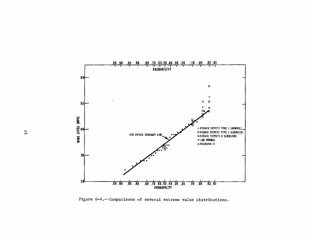
"' l.J>

60

50

: .... ~ C>

~40 .... "' C>

i!5 ;o:

3D

.99 .98 .95 .90 .80 .70 .60,.50.40 .30 .20 .10 .05 .02 .01

PROBABILITY

EYE FITTED STRAIGHT LINE

0

X

0 0

X

"

x FISHER TIPPETT TYPE I !GUMBEL) OFISHER TIPPETT TYPE I ILIEBLEINI o FISHER TIPPETT II ILIEBLEINI '1 LOG NORMAL "'PEARSON Ill

201~------~~~.&~~~~-r.~~~~--t.~--~~------~ .99 .98 .95 .90 .80 .70 .60 .50 .40 .30 .20 .10 .05 .02 .01 PROBABILITY

Figure 6-4.--Comparisons of several extreme value distributions.

60

1 •"' 1 • 55

--2 ,.­.. .,. .... u

3•"'

NORMAL DAILY TEMPERATURES ~FOR FARGO AND MINOT

DURATION [DAYS]

• YEAR

• FARGO J HIGHEST TEMPERATURES FOR INDICATED 6. MINOT DURATIONS. • WEEKLY MEAN TEMPERATURES OBTAINED FROM

DEPARTURES FROM NORMAL IN N. DAKOTA, MINNESOTA, WISC., AND EASTERN MONTANA [1934-1S70 I

5

Figure 6-5.--Adopted critical temperatures for snow-on-ground conditions.

46

30

30°~-.r--,r--,~-.--~---.---.---.--,---,

oo 2 4 6 8 10 DAYS

Figure 6-6.--Departure from normal temperatures for 1 to 10 days duration.

5o1---.--r--.-----.-..----.--.........--~

010 15 20 25 31 5 10 15 MARCH APRIL

Figure 6-7.--Normal daily temperatures (basin averages).

20

105° 103° 101° 15°..Z::... 97°

51° + + + + +

20° 49° _,___

25°

45° 105°

I I

I I

+

RED RIVER BASIN

r------------' I I SOUTH DAKOTA

103° 101° 99"

Figure 6-8.--Normal daily temperatures (oF) •

105° 103° 101° 3 5 099° 97°

51" + + + +

I

I I

I NORTH DAKOTA I

I + + +

I

r------------·~ I SOUTH DAKOTA

45 " ....... ---~-45 ° 103° 101° 77-

95° 93"

I I -15° I+ 51°

49"

95°

Harch.

95" 93°

I I

I+ 51°

95°

Figure 6-9.--Normal daily temperatures (°F). April.

48

110"

so· +

105" 100" ... ,.. +so·

+ + +

-,----------I I ,L_ I .,. ' +

Figure 6-lOa.--Outer isohyets of major

105°

+

' I ' I

April

100"

storms.

... ,..

+

I j ______ ~

... +

Narch

See table 6-4 for -----------~ { · storm identific~tion ·--"-,'\ ~---_________ _j___ l

40" ' I ·~--------·------+----------+ I 1011· J.

+

"· ,.. ' .

so•

and

85"

+

Figure 6-lOb.--Outer isohyets of major Harch and April storms.

49

BO•

...

... ' 1-·

,.85" --~

:z:: ,_ ::E

Cl ... ... ,_ V> Cl z: ~

~

0

,_ :!!!: C> .... ~ ~

"" ~

"' => ,_ ... "' ~ .... ::E ~ ,_

40

• • Snow cover periods

with high temperatures (fig. 6-5)

30 X April storms (table 6-4)

20

• • • • • X X X

X X X X

10

o~--~~2~--~--4~--~--&~~~~8~~~~1~0--~--~12

DAYS

Figure 6-11.--Durational variation of windspeed.

10

5

2 3 DAY PRIOR DAY AFTER

Figure 6-12.--Recommended temperature-dew point differences for PMP storm.

50

Chapter 7

SNOWPACK AVAILABLE FOR SPRING MELT

Introduction

A first approximation of snowpack available for spring melt may be obtained from Weather Bureau Technical Paper No. 50 (U.S. Weather Bureau 1964). Based on records prior to 1964, the paper gives maps of station maximum water equivalent of snow on the ground during March 1-15 and March 16-31 for SO-, 20-, 10-, 4-, 2- and 1-percent probability levels. For example, the average station value at the 1-percent probability level for the Red River drainage during March 16-31, is 7.6 in. The purpose of this study is to develop estimates of a reasonably severe areal snowpack without specifying the fre­quency, based on observed severe cases.

Data

Basic data used in Technical Paper No. 50 (U.S. Weather Bureau 1964) were used to determine the dates that provided the greatest observed station snowpacks of record up to 1964. Many of the greatest observed cases came during the March 16-31, 1962, and March 16-31, 1951, periods. In addition, three cases of large snowpacks were selected from recent years not covered in Technical Paper No. SO. Table 7-1 lists the six cases and other informa­tion. Data for 1952 came from Weather Bureau Technical Paper No. 23 (U.S. Weather Bureau 1954); for 1965 from ESSA Technical Report No. liB-4 (Paulhus 1967) and for 1969 from NOAA Technical Report NWS 13 (Paulhus 1971).

For the two cases selected from Technical Paper No. SO, the highest snow­packs, in terms of water equivalent, for each observation station during the 15-day period were plotted on maps. These then were analyzed and isopleths of water equivalent drawn. For these two cases the highest water equivalent within a 15-day period was selected for each station; thus the analyzed map is probably a slight maximization of actual water equivalent for any single day. Maps of water equivalent for the other four dates were already available from the cited publications.

Figures 7-la and 7-lb give the outer isopleths of snowpack (water equivalent) for each date or period. Maximum areal depths of water equiva­lent were then computed and curves of maximum depth of water equivalent versus area determined for each case. Figure 7-2 shows these resulting curves.

Most of the outlines of high snow-on-ground situations are south of the two drainages, and direct transposition of these unadjusted snowpacks to the two basins would not be warranted. Hence, we adjusted the maximum

51

areal values on the basis of station 1-percent probability water equivalent maps (U.S. Weather Bureau 1964). The ratio of the average !-percent proba­bility value over the basin to the average !-percent probability value where the snowpack was observed is the adjustment applied. Table 7-1 gives these adjustments for transposition to the basins.

Figure 7-3 shows the resulting depth-area curves of maximum water equiva­lent for each of the six cases after adjustment to the Red River Basin. Figure 7-4 shows the adjusted values for the Souris River drainage. The greatest depths for both basins for any size area came from the March 14, 1969, values of snow on the ground.

Maximum Snowpack From Synthetic Season Approach

An alternate method of estimating maximum spring snowpack, termed the synthetic season approach, is to combine the highest precipitation of record for set time increments of the precipitation accumulation season. For example, the highest November precipitation of record added to the highest December precipitation, etc., on to the highest March precipitation would give a synthetic seas·on of high precipitation. This procedure has been used in Hydrometeorological Report No. 42 (U.S. Weather Bureau 1966) for the Yukon River Basin of Alaska and in numerous studies for basins in Canada (Bruce 1962). The duration of the time increments of precipitation used in this procedure necessarily has a large effect on the seasonal accumulated precipitation. As the time increment becomes shorter, the accumulated precipitation becomes larger. Because of this variation, the synthetic­season approach is normally used in conjunction with other methods. The synthetic season approach was applied in this study using monthly precipi­tation (1931-60) averaged over state divisions. The subdivisions used are heavily outlined in figure 7-5. The Northwest Division of North Dakota was chosen as representative of the Souris drainage; the other three divisions (Northeast and East Central North Dakota and Northwest Minnesota) as repre­sentative of the Red River drainage. For the various division sizes, the highest adjusted water-equivalent values from figures 7-3 and 7-4 are com­pared with the synthetic ·season approach in the last two columns in table 7-2. Transpositions of actual snowpacks give greater depths than the synthetic season approach for each state division. We recommend the greatest adjusted water-equivalent depths of figures 7-3 and 7-4 for the March 15 PMP storm for the two drainages of this study.

Seasonal Variation

The recommended water equivalents are considered appropriate for March 15. As the season progresses it would be difficult to maintain these depths. Data from the March 1969 snowpacks (extrapolated) indicate a decrease of approximately 40 percent by April 15. A similar extrapolation of the station !-percent probability values (U.S. Weather Bureau 1964) indicates a reduction of 56 percent. We recommend April 15 values that are 50 percent of the March 15 depths. Depths of intermediate dates may be interpolated.

52

Table 7-1.--Dates or periods of high-water equivalent in North Central States and transposition adjustments (see figs. 7-la and 7-lb for location of snowpacks)

Date Adjustment for Adjustment for Red River Drainage Souris Drainage

1 Mar. 30, 1965 0.58 0.32 2 Mar. 14, 1969 1.27 0.70 3 Mar. 28, 1969 1.31 o. 72 4 Mar. 20, 1952 1.38 0.76 5 Mar. 16-31, 1951* 0.76 0.42 6 Mar. 16-31, 1962* 0.81 0.45

*Water equivalents based on highest station values for any day of period.

Table 7-2.--Comparison of highest November through March precipitation (1931-60) for selected State divisions with adopted maximum snowpacks by transposition

State and division

North Dakota

Northwest Division

Northeast Division

East Central Division

Minnesota

Northwest Division

*See figure 7-5

Normal precip.

(in.)

2.3

3.0

2.9

3.5

Synthetic season of

highest monthly precip. for each month (Nov-March)

Highest Actual seasonal

precip. (in.) and season (in.)

4.1 (1948-49) 6.1

5.4 (1944-45) 9.3

5.0 (1947-48) 9.3

5.3 (1949-50) 9.0

for division location and area.

53

Adjusted Snowpacks from

figs. 7-3 or 7-4 for same size of

area as state divisions

(in.)*

6.6

12.0

12.4

11.4

95'

+ +

85"

+

--,--'

Figure 7-la.--Outer isopleths of snowpack water equivalent (in.) for selected cases.

95' 90'

+ + + ---'

I ' I

-, { " "{,

r---------\-#4 I,, "'I • . .,. -+---! I / ,... l / . ) +f // /• ~'-1-' •• '.··)·--::-._

' 4"/ .... IL' /'.,. ~· . I .... .... .. . . r . . . ·. . . .....

I 1:' ··.\•.···"•.:: .'·'>). "·· I ,_, •• , • • •: ·~------,.!.J.d

/-----~·-<:\. ·-·,,_/· ·~ . . ' . ' . ---_ _)__See table 7-1 fo~·. '"'('',, .•.. .' )

85'

+

I

50'

dates of snow pack \ )-40o cases. \ ------ '

~----+---- ~ 1050 JOQO - -- ?5o 9'oo

I , .. iJ>

Figure 7-lb.--Outer isopleths of snowpack water equivalent (in.) for selected cases.

54

"' "'

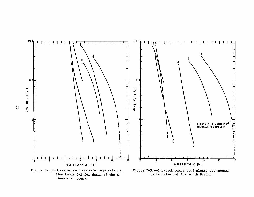
1DDD 6 5

iiE d ~

~

= = :; ~ c

4'

1DD

\ I I I I I I

t 4 6 I

I I I I

I I I I I I I I I I I I I I I I I I I I 2 D 2 4 6 8 1D

WATER EQUIVALENT JIN J

Figure 7-2.--0bserved maximum water equivalents. (See table 7-1 for dates of the 6 snowpack cases).

' l 12

I DO De 1 I I_ ~ I I I I I I I I I I I I I I I I I I I I

2 3

4

1 DD

-iiE d ~

~

= = :; ~ c

I 1\ \ 3

1 D

~ \\ \ RECOMMENDED MAXIMUM jlf SNDWPACK FDR MARCN 15

t 6

4

I I I 1 I I I I I I I I I 1 I 1 I I I I I 2 4 6 8 1 D 12

WATER EQUIVALENT

Figure 7-3.--Snowpack water equivalents transposed to Red River of the North Basin.

I II

I 2 14

"' 0'<

1000 1 1 1 1 _,,. 1 1 1 I I I I I I I I I I I I

-101

:E

= ~

~

= =

c ~

~ c

1Df.-

10

\\

. II

2

2 3

4

. I

6 \ 4

4

RECOMMENDED MAXIMUM SNOWPACK FOR MARCH 15

~

3 \ I I I I I I I I I I I

WATER EQUIVALENT (IN]

Figure 7-4.--Snowpack water equivalents transposed to Souris River Basin.

10

~ ... \ ...

r-... "' R BASIN .,..._) SOURIS ~VE RED RIVER OF

I I THE NORTH BASIN.\ ,. \ , ~.....,.._ - - . ~-- - - ' -·,_/'-'... \ ,--... ~ ~ /' ~;;;~~ESJ \ /tTHEASl ' '...,.., \,-"\._-"-::,?

' I NORTH ) ' • _, ~, WEST ,._, /

- ' I ' I '

NORTH DAKOTA EAST

ltENTRALI

' L I .....

--- ~I ------' ' ~

APPROX. ' Dl VISION AREA (SQ Ml ) I·

NORTH DAKOTA

I MINNESOTA ,

( )

/ '

NORTHWEST 9000 I """\.__ NORTHEAST 8800 I ,_ EAST CENTRAL S600 ')_

MINNESOTA ~-----------~ NORTHWEST 13,000

Figure 7-5.--State divisions used for synthetic season approach to maximum snowpack.

Chapter 8

PROCEDURE FOR USING CRITERIA WITH EXAMPLE

Introduction

Use of the various figures and charts to obtain PMP estimates and the recommended snowmelt criteria are summarized in this chapter. This is fol­lowed by an example for a selected subbasin.

A. All-season PMP

1. Basic PMP values

a. Enter figure 3-1 with area of subbasin. Read PMP for the given durations on abscissa.

(For Souris River subbasins, reduce PMP values by 10 percent)

2. Ge~graphic adjustment

a. Outline subbasin on figure 4-2c. Estimate average percent geographic adjustment.

(Use figure 4-3c for Souris River subbasins)

b. Multiply durational values of la by this adjustment.

3. 6-hr incremental PMP

a. Plot values of 2b on a time scale. From a smooth curve connecting the values, interpolate for 42-, 54-, and 66-hr PMP.

b. Successively subtract durational PMP to obtain 6-hr incre­mental PMP.

4. Sequence of 6-hr PMP increments

a. Arrange 6-hr PMP increments in accordance with guidelines in chapter 5, page 24.

5. Areal distribution

(Assume uniform areal distribution of all 6-hr PMP increments for subbasins less than 1,000 sq mi in area. For subbasins larger

57

than 1,000 sq mi use the isohyetal two greatest 6-hr PMP increments. for remaining PMP increments.)

pattern, figure 5-l, for the Use uniform areal distribution

a. Enter figure 5-3 with area of subbasin. Read isohyetal values on abscissa for greatest 6-hr PMP increment in percent of sub­basin 6-hr PMP. Use figure 5-4 in a similar manner to obtain isohyet values for the 2nd greatest 6-hr PMP increment.

b. Multiply percents from figure 5-3 by greatest 6-hr PMP increment, step 3b, to obtain isohyetal values in inches. Multiply percents from figure 5-4 by second greatest 6-hr PMP increment, step 3b, to obtain isohyetal values for second greatest 6-hr PMP increment.

6. Adjustment of PMP for orientation of isohyetal pattern

a. Lay isohyetal pattern, figure 5-l, over subbasin obtain greatest volume of rain within subbasin. for other possible more critical orientations.)

so as to (Note step e

b. From table 5-2 determine percent adjustment for this orientation.

c. Multiply isohyetal values of step 5b by the percent adjustment to obtain final isohyetal values for the two greatest 6-hr PMP increments.

d. Multiply remaining 6-hr PMP increments, step 3b, by the same percent adjustment.

e. Test fitting the isohyetal pattern over the subbasin within the no adjustment limits of table 5-2 and for a more critical hydrologic centering to compare resulting floods. Use most critical isohyetal placement.

B. Seasonal variation of PMP

1. Determine geographic adjustment for March 15 and April 15 for subbasin from figures 4-2a and 4-2b, respectively. Interpolate for desired date of PMP.

(For Souris River drainage use figures 4-3a and 4-3b)

2. Use table 4-2 to obtain seasonal adjustment for center of Red River of the North and Souris River drainages. Interpolate for desired date.

58

3. Multiply geographical adjustment (Bl) by seasonal adjustment (B2). This product, divided by the all-season geographical adjustment (A2a) gives a factor for multiplying all-season isohyet values (A6c) to obtain isohyet values for the date selected.

4. Multiply remaining 6-hr PMP increments (A3b) by the same factor as in 3 above.

C. Snowmelt Criteria

1. Winds

a. Daily average winds for 10 days prior to storm are given in table 6-5.

b. Six-hour average winds during PMP storm are given in table 6-2b. Arrange these into same sequential order as rainfall (see A4a).

c. Daily average winds for 3 days after storm given in table 6-6.

2. Temperatures

a. Prior to storm

(1) Determine normal daily temperatures (March 15 and April 15) over subbasin from figures 6-8 and 6-9. Interpolate for required date prior to selected day for beginning of storm.

(2) Daily departures from normal temperatures for the 10 days prior to storm given in table 6-3 for three dates. Interpolate for required date.

(3) Daily temperatures for 10 days prior to storm obtained by adding normal subbasin temperature, item 2a (1), to each temperature departure, item 2a (2).

b. During storm (Temperature = dew point)

(1) Determine average 12-hr persisting dew point (March 15 and April 15) over subbasin from figures 6-1 and 6-2. Interpolate for required date.

(2)

(3)

(4)

Determine precipitable water (W ) for this dew point from figure 6-3. P

Multiply W by percents of table 6-1 to obtain W correspond~ng to 6-hr incremental dew points. P

Enter figure 6-3 with W values to obtain 6-hr dew points. p

59

(5) Adjust these values to elevation of the basin by decreasing at the rate of 3"F per 1,000 ft above sea level.

(6) Arrange elevation adjusted 6-hr values in the same sequential order as rainfall (item A4a).

c. After storm

(1) Average daily temperatures are 7"F lower on the 1st day, 9"F on the 2nd, and lO"F on the 3rd day after the storm than on the last day of the storm.

3. Dew Points

a. Prior to storm

(1) Subtract indicated degrees given in figure 6-12, from each daily average temperature of C2a (3).

b. During storm

(1) Same as temperatures, see C2b (6)

c. After storm

(1) Daily dew points are 6"F lower than temperatures, see item C2c (1).

Note: If half-day temperatures and dew point are required, add and subtract 6"F from daily averages.

D. Maximum Snowpack Water Equivalent

1. Read value of recommended maximum snowpack water equivalent from figure 7-3 for the area of the subbasin. (Use fig. 7-4 for Souris River Basin). This is for March 15.

2. For April 15 use 50 percent of March 15 value. Interpolate for required date.

Example

The_drainage of the Red Lake River above Crookston, Minn., a 5280-sq-mi subbasin, is used here as an example of how developed criteria may be applied. For snowmelt computations, the average elevation of this basin is assumed to be 1,500 ft. In actual problems concerned with larger basins, the criteria may be determined for elevation bands, if desired.

The identification letters and numbers in the example correspond to the steps in the outlined procedure.

60

A. All-season PMP

Duration (hr) 6 12 18 24 30 36 42 48 54 60 66 72

PMP (in.) 1. Basic PMP values (fig. 3-1) 7.7 9.6 10.8 11.6 12.4 13.1 - 14.3 - 15.1 - 15.8

2. Geographic adjustment

a. From figure 4-2c=l00 percent

b. Geographically adjusted PMP values of Al times 100 percent 7.7 9.6 10.8 11.6 12.4 13.1 - 14.3 - 15.1 - 15.8

3. 6-hr incremental PHP

a- a. Geographically adjusted .... PMP with interpolations 7.7 9.6 10.8 11.6 12.4 13.1 13.7 14.3 14.7 15.1 15.5 15.8

6-hr period (!=highest, 12= lowest)

1 2 3 4 5 6 7 8 9 10 11 12 b. 6-hr incremental PMP

(in.) 7.7 1.9 1.2 0.8 0.8 0. 7 0.6 0.6 0.4 0.4 0.4 0.3

4. Sequence of 6-hr PXP increments

Time (hr) from beginning of storm 6 12 18 24 30 36 42 48 54 60 66 72

a. A sequence selected Sequence of 6-hr increments from chapter 5, p. 24 8 6 5 7 4 2 1 3 9 10 11 12

6-hr PHP increm·ents (in.) 0.6 0.7 0.8 0.6 0.8 1.9 7.7 1.2 0.4 0.4 0.4 0.3

5. Areal distribution

(Assume uniform areal distribution for all 6-hr increments except the two greatest.)

Isohyet p A B c D E F

a. Isohyet values in percent of greatest 6-hr PMP increment from figure 5-3 for 5,280 sq mi 200 179 157 130 80 47 26

Isohyet values in percent of 2nd greatest 6-hr PMP increment from figure 5-4 22i 164 137 110 88 75 63

b. Isohyet values (in.) for greatest 6-hr PMP incre-ment (percents of a times

a- 7. 7) 15.4 13.8 12.1 10.0 6.2 3.6 2.0 N

Isohyet values (in.) for 2nd greatest 6-hr PMP increment (percents of a times 1. 9) 4.2 3.1 2.6 2.1 1.7 1.4 1.2

6. Adjustment for orientation of isohyetal pattern

a & b. Orientation of isohyetal pattern figure 5-l for best fit to subbasin outline, 80"-260", indicates no reduction in PMP (table 5-2).

c & d. Final isohyet values for all-season PMP are given in 5b. Other 6-hr PMP increments are given in A4a.

e. For this example, it is assumed the best fit orientation is the most critical.

a­"'

B. Seasonal variation of PHP

(PHP criteria in this example are determined for April 15.)

1. Geographical adjustment over subbasin for April 15 (fig. 4-2b)=l01 percent

2. Seasonal adjustment for April 15 from table 4-2=72 percent

3. Geographical adjustment times seasonal adjustment (10lx72)=73 percent; 73 percent divided by all-season geographic adjustment (the latter is 100 percent from A2a)=73 percent

April 15 isohyet values (in.) (values of ASh times 73 percent)

4.

Greatest 6-hr PHP increment

2nd greatest 6-hr PHP increment

All-season incremental PHP times 0.73, arranged in same sequence as for all-season PHP (see A4a)

C. Snowmelt criteria

1. Winds

a. Daily average winds prior to storm (from table 6-5)

b. 6-hr winds during storm (table 6-2b), arranged in same sequence as rainfall (see A4a)

p

11.2

3.1

8 6

0.4 0.5

10 9

10 10

8 6

19 21

Isohyet A ll c D E

10.1 8.8 7.3 4.5 2.6

2.3 1.9 1.5 1.2 1.0

6-hr period 5 7 4 2 1 3 9 10 April 15 6-hr incremental PHP (in.)

0.6 0.4 0.6 1.4 5.6 0.9 0.3 0.3

Day prior to storm 8 7 6 5 4 3

Hindspeed (mph) 12 13 13 14 15 15

Sequence of 6-hr increments 5 7 4 2 1 3 9 10

Windspeed (mph) 23 21 25 31 37 27 18 17

F

1.5

0.9

11 12

0.3 0.2

2 1

18 31

11 12

16 14

a-....

c. Daily average winds after storm (from table 6--6-)---

2. Temperatures

a. Prior to storm

1

28

Day after storm 2

Windspeed (mph) 10

3

12

(1) Normal daily temperature over subbasin for April (fig. 6-9) = 39° F

Day prior to storm 10 9 8 7 6 5 4 3

(2) Daily dep. from normal temp, ( °F) for April 15 Temperature (°F) (table 6-3) 3 3 3 3 4 5 7 8

(3) Temp. dep. added Temperature (°F) to 39° F 42 42 42 42 43 44 46 47

b. During storm (temperatures = dew points)

(1) 12-hr persisting dew point, figure 6-2, for subbasin= 60° F

(2) Precipitable water (W ) for this dew point from figure 6-3 is 1.41 in. p

6-hr period 1 2 3 4 5 6 7 8 9

(3) w~ times percents Wp (in.) o table 6-1 1.51 1.41 1.33 1.27 1.21 1.15 1.11 1.07 1.04

(4) Dew points corresponding to OF W , figure 6-3 61.8 60.5 59.2 58.3 57.4 56.5 55.7 55.0 54.4

p

(5) Dew points reduced to 1,500 ft elev. OF oo F 11,ooo ft) 57.3 56.0 54.7 53.8 52.9 52.0 51.2 50.5 49.9

2 1

14 22

53 61

10 11 12

1.01 .99 .96

53.8 53.3 52.7

49.3 48.8 48.2

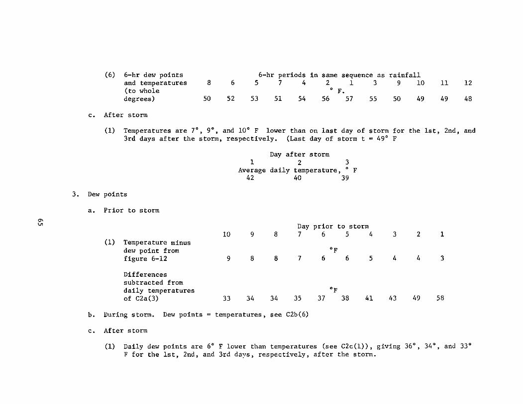
3.

a-l.n

c.

(6) 6-hr dew points 6-hr periods in same sequence as rainfall and temperatures 8 6 5 7 4 2 1 3 9 10 11 12 (to whole o F. degrees) 50 52 53 51 54 56 57 55 50 49 49 48

After storm

(1) Temperatures are 7°, 9°, and 10° F lower than on last day of storm for the 1st, 2nd, and 3rd days after the storm, respectively. (Last day of storm t = 49° F

1 Day after storm

2 3 Average daily temperature, o F

42 40 39

Dew points

a. Prior to storm

Day prior to storm 10 9 8 7 6 5 4 3 2 1

(1) Temperature minus dew point from OF figure 6-12 9 8 8 7 6 6 5 4 4 3

Differences subtracted from daily temperatures OF of C2a(3) 33 34 34 35 37 38 41 43 49 58

b. During storm. Dew points= temperatures, see C2b(6)

c. After storm

(1) Daily dew points are 6° F lower than temperatures (see C2c(l)), giving 36°, 34°, and 33° F for the 1st, 2nd, and 3rd days, respectively, after the storm.

"' "'

D. Maximum snowpack water equivalent

1. Maximum depth of March 15 water equivalent from figure 7-3 for 5,280 sq mi is 12.5 in.

2. Use 50 percent of March 15 for April 15 values, giving 6.3 in.

ACKNOWLEDGMENTS

The author is grateful for the help of numerous members of the Hydro­meteorological Branch staff in the course of this study. Francis Schwarz made helpful suggestions in developing the snowmelt criteria and in editing the report. Calvin Cochrane, William Swayne. and Roger Watkins carried out details of the PMP estimates and isohyetal values. Marshall Hansen carried out the tests of the frequency distributions. Miriam McCarty, Marion Choate, Wallace Brewer and Ray Evans made detailed computations, data extractions, many charts and maps. Typing was done by Christina Ebner, Edna Grooms and Cora Ludwig. Finally, many suggestions were made by John Miller, Chief of Water Management Information Division, Office of Hydrology, National Weather Service.

67

REFERENCES

Atmospheric Environment Service, "Storm Rainfall in Canada," Downsview, Ontario, Canada, 1961,

Bruce, J, P., "Snowmelt Contributions to Maximum Floods," Proceedings Eastern Snow Conference, pp. 85-103, 1962,

Canada, Department of Transport, Meteorological Branch, "Maximum Precipi­tation Reported on any Observation Day, 1931-1958," Summary of data through 1958,

Canada, Department of Transport, Meteorological Branch, "Atlas of Climatic Maps," 1967.

Chow, V. T., Handbook of Applied Hydrology, McGraw-Hill, New York, 1964,

Corps of Engineers, u. S. Army, "Storm Rainfall in the United States," Washington, D. C,, 1945-.

Environmental Data Service, "Climatic Atlas of the United States," ESSA, U.S. Department of Commerce, 1968,

Environmental Data Service, "Maximum Persisting 12-hour 1000-mb Dew Points (°F) Monthly and of Record," Climatic Atlas of the United States, ESSA, U, S, Department of Commerce, 1968.

Environmental Data Service, "Weekly Weather and Crop Bulletins," ESSA, U.S. Department of Commerce and U,S. Department of Agriculture, Statistical Reporting Service, Washington, D,C., 1970 (weekly publication),

Gumbel, E, J., "Statistics of Extremes," Columbia University Press, New York, 1958.

Lieblein, J., "A New Method of Analyzing Extreme Value Data," NACA Technical Note 3053, 1954,

Myers, V, A., ·~eteorological Estimation of Extreme Precipitation for Spillway Design Floods," Weather Bureau Technical Memorandum, WBTM-HYDR0-5, ESSA, U, S, Department of Commerce, 1967,

Paulhus, J,L.H., and Nelson, E,R., "The March-May 1965 Floods in the Upper Mississippi, Missouri, and Red River of the North Basins," ESSA Technical Report WB-4, 1967,

Paulhus, J,L,H,, "The March-April 1969 Snowmelt Floods in the Red River of the North, Upper Mississippi and Missouri Basins," NOAA Technical Report NWS 13, 1971

68

REFERENCES (Cont'd)

Schwarz, F, K,, "Probable Maximum and TVA Precipitation Estimates for the Drainage above Kentucky Dam and Below the Major Tributary Reservoirs," unpublished manuscript to the Tennessee Valley Authority, August 1970.

Thom, H,C,S,, "Some Methods of Climatological Analysis," World Meteorological Organization, Technical Note 81, 1966.

U,S, Weather Bureau, "Highest Persisting Dew Points in the Western United States," Technical Paper No. 5, 1948.

U.S. Weather Bureau Technical Paper No. 16, "Maximum 24-Hour Precipitation in the United States," January 1952a,

U,S, Weather Bureau, "Kansas-Missouri Floods of June-July 1951," Technical Paper No, 17, July 1952b.

U,S, Weather Bureau, "Preliminary Estimate of Probable Maximum Precipitation over the Red Lake River Basin above Crookston, Minn. and the Huot Reservoir Site," Memorandum to Office of the Chief, Corps of Engineers, October 1952c,

U.S. Weather Bureau, "Normal Weather Charts for the Northern Hemisphere," Technical Paper No, 21, 1952d.

U,S, Weather Bureau, "Floods of April 1952--Upper Mississippi, Missouri, Red River of the North," Technical Paper No. 23, 1954,

U,S, Weat'Jer Bureau, "Seasonal Variation of the Probable Maximum Precipita­tion East of the 105th Meridian for Areas from 10 to 1000 Square Miles and Durations of 6, 12, 24 and 48 Hours," Hydrometeorological Report No, 33, 1956.

U.S. Weather Bureau, "Decennial Census of the United States Climate, Monthly Averages for State Climatic Divisions, 1931-1960," Washington, D,C,, 1963.

U.S. Weather Bureau, "Frequency of Maximum Water Equivalent of March Snow Cover in North Central United States," Technical Paper No, 50, 1964,

U,S, Weather Bureau, "Meteorological Conditions for the Probable Maximum Flood on the Yukon River above Rampart, Alaska," Hydrometeorological Report No, 42, ESSA, U, S, Department of Commerce, 1966,

U,S, Weather Bureau, "Probable Maximum Precipitation over South Platte River, Colorado, and Minnesota River, Minnesota," Hydrometeorological Report No, 44, ESSA, U. S. Department of Commerce, Washington, D. C., 1969.

U.S. Weather Bureau, "Climatological Data for the United States by Sections," Washington, D.C., 1970 (monthly publication),

~U.S. GOVERNMENT PRINTING OFFICE: 1973-511-327/294

Nl& -------------· Mall to: National Technic:altntormalion Service

DEPARTMENT OF COMMERCE P.O. Box 1553. Springtield, Virginia 22151

Please send me ___ copies ol INDEXED BIBLIOGRAPHY OF THERMAL EFFECTS LITERATURE-2 at SID each. $12.50 foreign ORNL-NSIC 97. 0 Check here lormicroliche. Please send me ___ copies ol INDEXED BIBLIOGRAPHY ON ENVIRONMENTAL MONITORING FOR RADIOACTIVITY at 510.00 each, 512.50 foreign. ORNL·NSIC 101. Check here lor microfiche. Please send me ___ copies of INDEXED BIBLIOGRAPHY ON NUCLEAR FACILITY SITING at 510.00 each. 512.50 roreign. OANL-NSIC 105. 0 Check h.ere lor microfiche. Please send me ___ copies ol COMPILATION Of NUCLEAR STANDARDS. BUJ EDITION. 1971- Part 1: United States Activities and Part II: NaHan at (excluding U.S.) and rntema!lonal A~ivities at 522.00 each set 524_50 !orelgn, ORNL-NSIC Part I 98 and Part 11102. 0 Check here lormicrotiche. Please send me ___ copies ol SUMMARY OF RECENT LEGISLATIVE ANO REGULA· TORY ACTIVITIES AFFECTING THE ENVIRONMENTAL QUALITY OF NUCLEAR FACILITIES atS10.00 each. S12_50 foreign. ORNL·NS!C 93. 0 Check here lor microfiche. Method ol Paymenl

0 ChargetomyNTISdeposit account no. :;-;=occ==-0 Bill me (not applicable 1o foreign orders). Add 50~ each till e. 0 HereismychecklorS .

'""'-------------------------------------------Address ____________________ _

City.State.ZiP'-------------------­

-----------------• Nuclear Materials Problems? Here are five answers.

1 ''Indexed Bibliography ofThennal Effects Literature··- a compil-• ation and annotated bibliography of infonnation previously

published in technical literature on the subject of thennal dis­charges from power plants and their interaction with aquatic ecology. Included are an author index. keyword index, abstracts and the KWIC title index. Engineering aspects of thennal effluent control are covered as well.

2 "Indexed Bibliography on Environmental Monitoring lor Radio-• activity'' -850 abstracts on environmental monitoring with back­

ground material to put monitoring problems in perspective. Lists pertinent references for a general environmental monitoring program emphasizing the nonnal operation of a nuclear facility.

3 ''Indexed Bibliography on Nuclear Facility Siting'' 900 abstracts • of documents pertaming to various phases of siting with emphasis

on the reports and questions that arise during the licensing of a nuclear plant. Keyword, author and KWIC indexes are provided.

4 "Compilation of Nuclear Standards 8th Edition, 1971: Part 1-• United States Activities; Part 11-National (excluding U.S.) and

International Activities"- all U. S .. national, and international nuclear standards with relevant regulations established by government agencies. Both volumes divided by organization and pennuted title.

5 ··summary of Recent Legislative and Regulatory Activities Affect-• ing the Environmental Quality of Nuclear Facilities" a summary

of recent legislative and regulatory activities, proposed and adopted Federal and State legislation which might affect the development of utilization of nuclear energy. Also included are execut1ve orders and water quality standards for all states.

Add these five references from the Nuclear Safety Information Center to your research library. Order now, by completing the coupon below.

IF YOU'RE RUSTY ON THE SUBJECT OF CORROSION, READTHESEI

Here are four Metals & Ceramics Information Center reports on corrosion and its treatment: •'The Corrosion of Metals In Marine Environments'" is· a current resource of information on the advanced metals and their use in hostile marine environment. It helps you to choose materials and equipment right for your job . .. Hot Corrosion in Gas Turbines'" deals primarily with the sulfidation problem and explains major testing methods and research. ••Oxidation of Iron, Nickel and Cobalt-base Alloys"' guides the engineer or metallurgist to current data on oxidation of the pure metals and their alloys, as well as of more complex eng'ineering alloys. .. Shot Peening for Improved Fatigue Properties and Stress Corrosion'" contains a summary of current peen­ing procedures, methods of control and improvement that can be achieved with these techniques.

Any one or all four of these studies can be invaluable to you in your research or in practical day-to-day operations. Put them on your shelf by filling out and returning the coupon below. ·-------------, Mall to: National Technical Information Service

GENTLEMEN,

Department of Commerce P.O. Box 1553 Springfield, Virginia 22151

0 Please send me copies of the M:CIC report THE CORROSION OF METALS IN MARINE ENVIRONMENTS. hard cover copies $12.50 each ($15.00 foreign) or----.,.., soft cover copies at $7.50 each ($10.00 foreign) AD· 712 585-H o< AD-712 585-S.

0 Send me ___ copies of the MCIC Report HOT CORRO-SION IN GAS TURBINES at $10.75 each ($13.25 fo<e;gn) AD-745 474.

0 Send me ___ copies of the MCIC report OXIDATION OF IRON, NICKEL AND COBALT-BASE ALLOYS at $10.75 each ($13.25 fo<elgn) AD-745 473.

0 Send me ___ copies of the MCIC report SHOT PEEN-ING FOR IMPROVED FATIGUE PROPERTIES AND STRESS CORROSION at $7.50 each ($10.00 fmeign) AD-735 409.

Please check method of payment.

D Charge to my NTIS account no. ------------,--0 Bill me {not applicable to foreign orders). Add 50¢ for each title. D Here is my check for ______________ _

Name-----------------------------------------

Tl~e. Organization _________________ _

Add~------------------------------------------

L ~-- J ----------------

NOW, a step-by-step guide to machining

\ ... _ ...

"THE MACHINING DATA OK"

This manual, recently revised and ex­ponded, is the largest volume of machin­ability information ever compiled. You'll find starting recommendations for all types of material removal operations and mote­rials. There ore machining recommenda­tions in tabular form which include many new materials as well as ten new opera­tions. Implementation information is also provided.

If you're a production plonn~r. tool oper­ator, machine shop supervisor, engineer, manufacturer, designer, researcher, or purchasing agent, you'll find this hondbool~ invaluable. So don't be without it. Order yours by completing and returning this handy order form.

I I I I I I I I I I I I I

GENTLEMEN, D Please send me copies of rhe MACHINING DATA

HANDOOOK, or $35 each ($37.50 foreign) CAD-742058)

Check One

0 Charge ro my NTIS occounr no. ---------0 Oill me (applicable to foreign orders). Add 50¢. 0 Here is my check for ___________ _

Nome ________________ _

Tirle _________________ _

Organization ______________ _

Address _______________ _

(;ry _________________ _

I Srare Zip _____ _

•-----------------A